2 School of Mechanical Engineering, Southwest Jiaotong University, Chengdu 610031, China; [email protected] Human-Oriented Built Environment Lab, School of Architecture, Civil and Environmental Engineering, École
Polytechnique Fédérale de Lausanne, CH-1015 Lausanne, Switzerland4 State Key Laboratory of Air-Conditioning Equipment and System Energy Conservation,
Zhuhai 519070, China; [email protected] Gree Electric Appliances, Inc. of Zhuhai, Zhuhai 519070, China* Correspondence: [email protected]
Abstract: Increased data monitoring enables the energy-efficient operation of air-conditioning sys-tems via data-mining. The latter is projected to have lesser consumption but more comprehensivediagnosis than traditional methods. Following the companion paper that proposed a systematicmethod for energy-saving potential calculations via data-mining, this article presents a detailed casestudy in an ice-storage air-conditioning system by employing the proposed method. Raw data werepreprocessed prior to recognizing the constant- and variable-speed devices in the system. Classifi-cation and regression tree algorithms were utilized to identify the operating modes of the system.The regression models between the energy-consumption and operating-state parameters of the ninepumps and two chillers were fitted. Furthermore, the constraints pertaining to system operation weresummarized. From the results, the particle swarm optimization method was applied to elucidatethe benchmark energy cost and the consequent cost savings potential. The cost savings potential forthe chiller plant room during the investigation duration of 59 d reached as high as 24.03%. The casestudy demonstrates the feasibility, effectiveness, and stability of the systematic approach. Furtherstudies can facilitate the development of corresponding control strategies based on the potentialanalysis results, to investigate better optimization algorithm, and visualize the analysis process.
Keywords: energy-saving potential; data-mining; recognition; optimization; operational data
1. Introduction
As reviewed in a companion paper [1], data mining can be a superior approach fordiagnosing the energy-saving potential of air-conditioning systems, particularly in the eraof data explosion. Compared to the traditional observation/question, test/calculation,and identification/resolution (OTI) method, energy-saving diagnosis based on data miningexhibits several advantages, including a more comprehensive analysis of energy-savingdiagnosis, reduced intervention of professional researchers, and less time. The companionpaper [1] proposed a systematic energy-saving diagnosis method for air conditioning sys-tems via data-mining. The proposed method consisted of seven steps: (1) data collection,(2) data preprocessing, (3) recognition of variable frequency equipment, (4) recognitionof system operation mode, (5) regression analysis of energy-consumption data, (6) con-straint analysis of the system during operation, and (7) analysis of energy-saving potential.To validate the proposed method and test its applicability and feasibility for application incomplicated air conditioning systems, this study mainly focuses on the technical details
of the method and the application of the method in a specific air conditioning system forenergy-saving diagnosis.
Previous studies have investigated the applicability of data-mining technologies inenergy-consumption-related investigations into air-conditioning systems and buildingenergy systems [2]. For instance, an artificial neural network (ANN) [3] and support vectormachine (SVM) [4] have been employed to diagnose chillers. Moreover, Gaussian processregression [5] and classification and regression trees (CART) [6] have been utilized todiagnose air handling units (AHUs). ANN [7] and an algorithm based on the recursivedeterministic perceptron neural network [8] have been utilized to detect pumps; symbolicaggregate approximation (SAX) have been applied to identify the operation patterns ofchillers [9] and heating, ventilating and air conditioning (HVAC) systems [10]. Few studieshave focused on the application of various data mining technologies, such as responsesurface methodology (RSM) and neural network (NN), in the diagnosis and optimization ofspecific components of HVAC systems and building energy systems. Li et al. [11] appliedclustering analysis and association mining to identify energy consumption patterns ofa variable refrigerant flow system. Neural network (NN) showed capability in optimiz-ing specific components, such as fluid in the refrigeration system [12]. Response surfacemethodology (RSM) was applied for the optimization of specific building energy systems,such as solar collector and reactor [13,14]. Global data mining, together with geographicinformation, has enabled country-wide optimization of building insulation for energysaving and mitigation of emissions [15]. However, the aforementioned case studies onlypertain to a specific step or optimization algorithm included in our systematic method.Newly proposed methods for energy saving analysis of HVAC systems, particularly theones focusing on systematic optimization, should be validated using case studies. Previ-ous studies that proposed new optimization methods for HVAC systems [16], buildingenergy systems [17], or specific components [18] were normally accompanied by casestudies for validation. Therefore, a comprehensive and detailed case study employing thenew systematic data-mining-based methodology is necessary to illustrate the method’sfeasibility.
This paper presents the second of two publications proposing a systematic method-ology to elucidate the energy-saving potential of an air conditioning system based ondata-mining. Following the proposed steps in the companion paper [1], a detailed casestudy was carried out in an air conditioning system coupled with an ice storage systemwith an air conditioning area of 30,000 m2. The details of specific data-mining technologiesin each step were introduced, and the energy-saving potential was calculated and analyzedusing the systematic method.
2. Methodology2.1. The Studied System
A five-floor commercial building was equipped with an air-conditioning system byemploying the new method. The building was located in Shenzhen, China, with a 30,000 m2
air conditioning area. The system was coupled with an ice-storage system (circulationmedium: glycol-water solution) to exploit the lower electricity price at night (Table A1 inAppendix A). As shown in Figure 1, the coupled system consisted of two chillers (Ch-1and Ch-2), three chilled-water pumps (ChWP-1, ChWP-2, and ChWP-3), three condensing-water pumps (CWP-1, CWP-2, and CWP-3), three glycol water pumps (GWP-1, GWP-2,and GWP-3), twelve ice-storage tanks, two plate heat exchangers, six cooling towers,and five air-handling units.
Energies 2021, 14, 86 3 of 22
Figure 1. Scheme of the studied air-conditioning system with the monitoring locations of the operation status.
The system had four operating modes, excluding the shutdown mode. Each modewas controlled based on the logic detailed in Table 1 for on/off control or the modulationof the chiller(s) and five valves (V1 to V5).
Energies 2021, 14, 86 4 of 22
Table 1. System operating modes and corresponding control logic.
Operating Modes CodesDevice Status
Chiller(s) V1 V2 V3 V4 V5
Ice build M1 On Off On Off On OffCooling by chiller(s) only M2 On On Off On Off Off
Cooling by ice only M3 Off Off On On Off OnCooling by ice with chiller(s) M4 On Modulate On On Modulate Off
2.2. Data Collection
A comprehensive data-monitoring platform was established for the air-conditioningsystem to monitor the electricity consumption of each component and the operating statusparameters of the system. The available monitoring points are indicated in Figure 1, and allthe points are summarized in Table 2, along with detailed information.
Table 2. Parameters monitored in the case system.
No. in Figure 1 Identifiers in Figure 1 Parameter Meaning and Unit Symbol
1 t_OA Outdoor air temperature (◦C) tOA2 t_cws Temperature of supply condensing water in main pipe (◦C) tcws3 t_cwr Temperature of return condensing water in main pipe (◦C) tcwr4 t_chws Temperature of supply chilled water in main pipe (◦C) tchws5 t_chwr Temperature of return chilled water in main pipe (◦C) tchwr6 t_chwCh-1 s Temperature of supply chilled water in chiller #1 (◦C) tchwCh-1 s7 t_chwCh-1r Temperature of return chilled water in chiller #1 (◦C) tchwCh-1r8 t_cwCh-1 s Temperature of supply condensing water in chiller #1 (◦C) tcwCh-1 s9 t_cwCh-1r Temperature of return condensing water in chiller #1 (◦C) tcwCh-1r
10 t_chwCh-2 s Temperature of supply chilled water in chiller #2 (◦C) tchwCh-2 s11 t_chwCh-2r Temperature of return chilled water in chiller #2 (◦C) tchwCh-2r12 t_cwCh-2 s Temperature of supply condensing water in chiller #2 (◦C) tcwCh-2 s13 t_cwCh-2r Temperature of return condensing water in chiller #2 (◦C) tcwCh-2r14 m_isIST Amount of ice in inventory (metric tons) misIST15 t_gwISTr Temperature of return glycol water to ice storage tanks (◦C) tgwISTr16 t_gwISTs Temperature of supply glycol water from ice storage tanks (◦C) tgwISTs17 t_PHEXp-1 s Temperature of supply water to premier side of plate heat exchanger #1 (◦C) tPHEXp-1 s18 t_PHEXp-1r Temperature of return water from premier side of plate heat exchanger #1 (◦C) tPHEXp-1r
19 t_PHEXs-1 s Temperature of supply water from secondary side of plate heat exchanger #1(◦C) tPHEXs-1 s
20 t_PHEXs-1r Temperature of return water to secondary side of plate heat exchanger #1 (◦C) tPHEXs-1r21 t_PHEXp-2 s Temperature of supply water to premier side of plate heat exchanger #2 (◦C) tPHEXp-2 s22 t_PHEXp-2r Temperature of return water from premier side of plate heat exchanger #2 (◦C) tPHEXp-2r
23 t_PHEXs-2 s Temperature of supply water from secondary side of plate heat exchanger #2(◦C) tPHEXs-2 s
24 t_PHEXs-2r Temperature of return water to secondary side of plate heat exchanger #2 (◦C) tPHEXs-2r25 R_V1 Opening of valve #1 (%) RV126 q_chw Chilled water flow in main pipe (L/s) qchw27 Q_CL Cooling load of the system (USRT) QCL28 W_CWP-1 Energy-consumption of condensing water pump #1 (kWh) WCWP-129 W_CWP-2 Energy-consumption of condensing water pump #2 (kWh) WCWP-230 W_CWP-3 Energy-consumption of condensing water pump #3 (kWh) WCWP-331 W_GWP-1 Energy-consumption of glycol water pump #1 (kWh) WGWP-132 W_GWP-2 Energy-consumption of glycol water pump #2 (kWh) WGWP-233 W_GWP-3 Energy-consumption of glycol water pump #3 (kWh) WGWP-334 W_ChWP-1 Energy-consumption of chilled water pump #1 (kWh) WChWP-135 W_ChWP-2 Energy-consumption of chilled water pump #2 (kWh) WChWP-236 W_ChWP-3 Energy-consumption of chilled water pump #3 (kWh) WChWP-337 W_AHU-1 Energy-consumption of air handling unit #1 (kWh) WAHU-138 W_AHU-2 Energy-consumption of air handling unit #2 (kWh) WAHU-239 W_AHU-3 Energy-consumption of air handling unit #3 (kWh) WAHU-340 W_AHU-4 Energy-consumption of air handling unit #4 (kWh) WAHU-441 W_AHU-5 Energy-consumption of air handling unit #5 (kWh) WAHU-542 W_Ch-1 Energy-consumption of chiller #1 (kWh) WCh-143 W_Ch-2 Energy-consumption of chiller #2 (kWh) WCh-244 W_ChPR Energy-consumption of chiller plant room (kWh) WChPR
Energies 2021, 14, 86 5 of 22
This study collected data from 22 July 2011 to 20 August 2013 at intervals of 1 h.All the data were utilized in this study for preprocessing and subsequent analyses. To betterexplain the specific types of data monitored by this study, Table A2 of Appendix A providesthe raw data for a full day (18 August 2013).
2.3. Data Preprocessing
The raw data were preprocessed to meet the needs of the subsequent analysis follow-ing the steps detailed in the subsequent sections.
2.3.1. Missing Data Preprocessing
• Listwise deletion: We deleted the data obtained before 22 June 2013, owing to abundantmissing values in the data from that period. This was done to ensure the continuity,isometry, and completeness of the data. Consequently, 1416 pairs of continuous time-series data for 59 consecutive days from 22 June to 19 August 2013 were retained forthe recognition of system operation mode in Section 2.5 and the energy cost-savingspotential analysis in Section 2.8.
• Pairwise deletion: In the regression analysis (Section 2.6) of energy consumption andflow rate for pumps, we deleted the energy-consumption data and the paired flowrate data in cases where either one or both values were missing. The same approachwas applied to the data used in the regression analysis for the chillers.
2.3.2. Data Cleaning
• Duplicate data cleaning: Consider the data obtained at 17:59:00 on 18 August 2013(see Table A2). Because the data were recorded at 1 h intervals, the data obtained at17:59:00 was considered to be a duplicate of the approaching hour (18:00:00) and wasdeleted.
• Data cleaning during the shutdown state: To faithfully reflect the distribution of energyconsumption in the operating state, before calculating the numerical characteristics ofthe energy-consumption data of the devices in Section 2.4, the data obtained during theshutdown state (i.e., when the energy consumption was zero) were deleted. The sameapproach was applied to the data used in Section 2.6 for regression analysis.
2.3.3. Data Extending
• Appending the code of system operation mode to the dataset: Following the recog-nition of the system operation mode (see Section 2.5), we added a column into thedataset with the corresponding operation-mode code (i.e., M1 to M4 in Table 1 andM0 for the shutdown mode) to facilitate the filtering of data by operation mode in therelevant analysis. For example, the chillers were regressed by cooling (correspondingto M2 and M4) and ice building (corresponding to M1) modes in Section 2.6.
• Temperature difference data extension: Typically, temperature differences are notdirectly captured and recorded during the data collection period but are frequentlyused in the analysis. Therefore, it is necessary to add temperature difference data tofacilitate direct recall for the relevant analysis (e.g., regression analysis in Section 2.7).For instance, we computed the temperature difference between the supply and thereturn chilled water (∆tchw = tchwr − tchws) as a new variable (∆tchw) and extended itto the case dataset. Similarly, for the temperature difference of the water supply andreturn chilled water of the chiller (∆tchwCh), the temperature difference between thewater supply and return condensing water of the chiller (∆tcwCh) were calculated andextended to the dataset.
2.3.4. Data Transformation
• Transformation of the units of measurement: The unit of the cooling load of thesystem in the case data was the US refrigeration ton (USRT). This unit pertains tothe cooling load (power nature) rather than the cooling quantity demand (energy
Energies 2021, 14, 86 6 of 22
nature); the former cannot be used directly in the subsequent analysis and calculation.Hence, the unit of USRT was converted to the système international (SI) unit ofkilowatts (kW). Because the data collection interval was 1 h, each value correspondedto the cooling quantity demand for that period. Therefore, the unit was furtherconverted to kilowatt-hour (kWh). In the case of chilled water flow (qchw), where therewere no more variables of the same type, the unit of liters per second (L/s) wasconverted to cubic meters per hour (m3/h) to avoid introducing too many conversionfactors in the subsequent analysis and calculation.
• Time interval labeling: For easier identification and more efficient data processing,the time interval was marked as period i. The one-to-one correspondences betweenthem are shown in Table A1 of Appendix A.
2.4. Recognition of Variable Speed Equipment
The regression analysis in Section 2.6 requires the matching of different fitting for-mulas for variable- and constant-speed motor-driven equipment; however, the variable-or constant-speed nature of equipment was not directly available in the monitoring data.Therefore, we applied the coefficient of the median, defined as the ratio of the differencebetween the maximum and median to the range, proposed in our previous study [19].The coefficient of the median aids in recognizing the two-speed types of motor-drivenequipment using their energy-consumption data. It was evident from the recognition re-sults that the four pumps (ChWP-1, ChWP-2, GWP-1, and GWP-2) and all the AHUs werevariable-speed equipment, whereas the remaining five pumps (CWP-1, CWP-2, CWP-3,ChWP-3, and GWP-3) and the two chillers (Ch-1 and Ch-2) were constant-speed devices.
2.5. Recognition of System-Operation Mode
The operation mode was not recorded for each period in the dataset. Therefore, it isnecessary to recognize or classify the system operation modes before relevant analysis.
As previously stated, in the studied air-conditioning system, there were five distinctoperation-modes: (a) shutdown (operation-mode code: M0), (b) ice build (M1), (c) coolingby chiller(s) only (M2), (d) cooling by ice only (M3), and (e) cooling by both chiller(s)and ice (M4). Moreover, the different operation modes of the system follow the clearcontrol logic shown in Table 1. While the data from the chillers and valve V1 can recognizemodes M1 to M4, they are insufficient to recognize mode M0, which is easily confusedwith M3. Therefore, the energy consumption of another energy-consuming equipmentis incorporated to ensure the correct recognition of mode M0. The energy-consumptiontypes of the involved devices, corresponding to different operation modes, are shown inTable 3. The use of electricity at night versus peak daytime hours can lead to large savingsin energy bills. This proves that the system primarily produces ice during the nighttimelow-tariff hours (23:00 to 07:00) when the building is closed to the public, and no cooling isrequired. The period i is therefore added to the mode recognition, which may be effectivein recognizing mode M1.
Table 3. Energy-consumption types of devices for different operation modes.
1 “0” indicates that the corresponding device is in a shutdown state. 2 “>0” indicates that the device is running.
Energies 2021, 14, 86 7 of 22
Classification is a method of building a categorization model by summarizing andrefining the patterns contained in existing data. Moreover, decision tree induction isa classical classification method with high accuracy and efficiency. To better elucidatethe data and incorporate background knowledge about it when building a decision tree,the classification and regression trees (CART) algorithm [6] with good interactivity waschosen to build the decision tree model for the study. CART uses a greedy method in whichthe decision tree is constructed using a top-down recursive partitioning approach. For theclassification of numerical input variables, CART measures the heterogeneity of the outputvariables by calculating the Gini index (Gini) [20] for each input variable and selects thesplitting variable that maximizes the reduction in heterogeneity (∆Gini). This variable andits split-point together form the splitting criterion. This procedure is repeated until thesplitting criteria for recognizing all operation modes are acquired, at the end of which thedecision tree construction is complete.
2.6. Regression Analysis of Energy-Consumption Data
The purpose of the regression analysis is to quantify the relationship between theenergy consumption of each energy-consuming device and its operation-state parame-ters. The obtained fitting model serves to reduce energy consumption by optimizingthe operation-state parameters while meeting the system load demands. The energy-consumption data of the cooling towers and operation-state parameters for AHUs werenot available in the dataset; therefore, follow-up analysis was performed only for theenergy-consuming equipment in the chiller plant room, which included the nine pumpsand two chillers.
2.6.1. Fitting Models for Regression Analysis
The nine pumps in the case study are categorized into constant- and variable-speedpumps based on the classification in Section 2.4, corresponding to different fitting models.Based on fluid dynamics, the fitting model of the energy consumption and flow rate for theconstant-speed centrifugal pumps is as follows:
W = β0 + β1q, (1)
where W represents the energy consumption of pump, kWh; q represents the flow rate ofthe pump, m3/h; and β0 and β1 are the two fitting coefficients and are dimensionless.
The fitting model for variable-speed centrifugal pumps can be determined as follows:
W = β1(q + β0)3. (2)
Several factors influence chiller-operating performance and energy consumption; anaccurate theoretical model can be developed via an in-depth analysis of chilling principles.However, this study of chiller-operating performance aims to exploit actual operation datato fit a real or near-real model that can predict energy consumption in the following energy-saving potential calculations. In some related studies, the mathematical models fromtwo well-known simulation software programs in the field, EnergyPlus (9.3.0, NationalRenewable Energy Laboratory, Golden, CO, USA) and TRNSYS (v. 17, Thermal EnergySystem Specialists, LLC, Madison, WI, USA ), were used directly or with appropriatemodifications based on the studies [21]. Herein, an improved model that can be effectivelyfitted as proposed in our previous study [22] is applied as follows:
where WCh represents the energy consumption of the chiller, kWh; QCh represents thecooling capacity of the chiller, kWh; tcwChr represents the temperature of return condensingwater of chiller, ◦C; ∆tchwCh represents temperature difference of water supply and thereturn chilled water of the chiller, ◦C; ∆tcwCh represents the temperature difference ofwater supply and the return condensing water of the chiller, ◦C; tchwChs represents thetemperature of water supply chilled water of the chiller, ◦C; β0 to β20 represent the fittingcoefficients and are dimensionless.
2.6.2. Data Preparation for Regression Analysis
Abnormal data have already been eliminated in the data preprocessing step (Section 2.3).However, the energy consumption data of each of the nine pumps were recorded in thecase dataset. The corresponding flow rate was recorded only for the main pipe of thechilled water loop (qchw), without a separate flow rate available for each pump. Therefore,it is crucial for the pump data to be processed in the following ways for regression analysis:
• Filter out the flow rate of the individual pump. Considering the chilled water flowrate (qchw) as an example, the data are filtered out with only one chilled water pumpin operation from all the data with flow rates (qchw) exceeding zero. The filtered flowdata and the corresponding pump energy consumption in the order of pump numberswere used for the respective regression analyses. For instance, a period when ChWP-1runs while ChWP-2 and ChWP-3 are shut down is determined, chilled water flowrate (qchw) is marked as the flow rate of ChWP-1 (qchw-1), and the process is repeatedto filter out the flow rate data for all ChWP-1. Subsequently, these filtered data areorganized into a subset of ChWP-1 for regression analysis. The relevant data subsetsfor ChWP-2 and ChWP-3 can be collated separately following the same procedure.
• Calculate the flow rate of the glycol water (qgw) and the flow rate of the condensingwater (qcw). In this study, ignoring the heat transfer loss of the system, Qchw = Qgw,the glycol water flow rate (qgw) can be calculated using the chilled water flow rate(qchw), the temperature difference between supply and return chilled water (∆tchw),and the temperature difference between supply and return glycol water solution(∆tgw) in the operating modes of M2, M3, and M4. Similarly, Qcw = QCh + WCh =Qchw + WCh, the condensing water flow rate (qcw) can be calculated using the chilledwater flow rate (qchw), the temperature difference between supply and return chilledwater (∆tchw), the energy consumption of the chillers, and the temperature differencebetween supply and return condensing water (∆tcw) in the operating mode of M2.Finally, using the first method, the relevant data subsets for each glycol water pumpand condensing water pump can be collated separately.
In addition, for chillers, after the preprocessing discussed in Section 2.3, the data forthe regression analysis no longer require further processing.
2.7. Constraint Analysis of System during Operation
The case system is subjected to the following constraints during operation, which willalso be taken into account in the energy-saving potential analysis.
2.7.1. Constraint on Supply and Demand of Cooling
During the cooling period in the operation modes of M2, M3, and M4, the coolingcapacity supplied by the chiller plant room must be sufficient to meet the cooling load ofthe case system, described by the following equation:
QCL(i) = QCh(i) + QcrIST(i), (4)
where QCL(i) represents the cooling load of the system during the period i, kWh; QCh(i)represents the cooling capacity supplied by chillers during period i, kWh; and Qcr
IST(i)represents the cooling capacity supplied by ice in the ice storage tanks during period i,kWh.
Energies 2021, 14, 86 9 of 22
2.7.2. Constraint on Cooling Capacity of Chillers
In the operation modes of M1, M2, and M4, the cooling capacity supplied by chillersshould not exceed the maximum cooling capacity of chillers at any time.
0 ≤ QCh(i) ≤ QmaxCh (i), (5)
where QmaxCh (i) represents the maximum cooling capacity of chiller during period i, kWh.
2.7.3. Constraints on ISTs
The sum of the accumulation of the cooling capacity in the ISTs and the currentremaining cooling capacity should not exceed the maximum accumulation of coolingcapacity of ISTs during any time:
0 ≤ QacIST(i) + Qre
IST(i) ≤ QmaxIST , (6)
where QacIST(i) represents the accumulation of cooling capacity in the ISTs during period i,
kWh; QreIST(i) represents the current remaining cooling capacity in the ISTs at the beginning
of period i, kWh; QmaxIST represents the maximum accumulation of cooling or cooling release
of ISTs during one cooling storage and release cycle, kWh.In the operation mode of M1, the accumulation of cooling capacity in the ISTs should
be equal to the cooling capacity supplied by the chillers during any time, ignoring the heattransfer loss.
QacIST(i) = QCh(i). (7)
Moreover, in the operation mode of M1, ISTs are constrained by their operationefficiency; the accumulation of cooling capacity cannot exceed the maximum coolingstorage speed in the current period.
0 ≤ QacIST(i) ≤ Qac,max
IST (i), (8)
where Qac,maxIST (i) represents the maximum cooling storage speed of ISTs during period
i, kWh.When cooling by ice (i.e., the operation mode of M3 and M4), the cooling release of
ISTs at any time should not exceed the remaining cooling capacity during that time.
0 ≤ QcrIST(i) ≤ Qre
IST(i), (9)
where QcrIST(i) represents the cooling release of ISTs during period i, kWh.
Similarly, the cooling release of ISTs cannot exceed the maximum cooling release speedin the current period.
0 ≤ QcrIST(i) ≤ Qcr,max
IST (i), (10)
where Qcr,maxIST (i) represents maximum cooling release speed of ISTs during period i, kWh.
In addition, the remaining cooling capacity of ISTs at any given time can be expressedas follows:
QreIST(i + 1) = Qre
IST(i) + QacIST(i)− Qcr
IST(i), (11)
where QreIST(i + 1) represents the remaining cooling capacity of ISTs at the beginning of the
period (i + 1), kWh.Note that these calculations only present expressions for the various constraints to be
called in the follow-up potential analysis step, while the specific data input and calculationwill be done automatically by the computer. The call of the equations is further describedin Section 2.8.2.
Energies 2021, 14, 86 10 of 22
2.8. Energy-Saving Potential Analysis2.8.1. Problem Definition and Principles of Potential Analysis
Generalized computational equations for energy and cost savings are presented in acompanion paper [1]. For the present case with multiple different tariffs in a day (Table A1in Appendix A), the energy cost savings for each day can be defined as follows:
∆J = Jactual − Jbenchmark =23
∑i=0
ei(Wactual(i)− Wbenchmark(i)), (12)
where ∆J represents the energy cost-saving of the air-conditioning system for one day, CNY;Jactual represents the actual energy costs of the air-conditioning system for one day, CNY;Jbenchmark is the benchmark energy cost of the air-conditioning system for one day, CNY;ei is the electricity price for period i, CNY/kWh; Wactual(i) is the actual energy consumptionof the air-conditioning system for the period i, kWh; and Wbenchmark(i) is the benchmarkenergy consumption of the air-conditioning system for the period i, kWh.
As previously mentioned, only energy consumption and performance data of equip-ment in the chiller plant room are available concurrently in this case, lacking the necessarydata related to cooling towers and AHUs. Therefore, this study focuses on the analysis andcalculation of the saving potential of the chiller plant room, summarized as follows:
The benchmark energy cost is the optimization result of the system operation. Someprinciples need to be followed to calculate the benchmark value.
• For each cooling storage and release cycle, the operation of the air conditioning systemshall be optimized and calculated according to the cooling load demand in each periodand the constraints described in Section 2.7;
• For each period of a cooling storage and release cycle, the operation mode shall bedetermined according to the cooling load demand and electricity tariff;
• For each period determined as the operation mode of M4, it is necessary to furtherdetermine the respective cooling supply ratios of the ice and chillers;
• For each set of parameters resulting from the above principles, the total energy cost ofthe chiller plant room was calculated according to the results of the regression analysisin Section 2.6;
• Search for the minimum energy costs as the benchmark energy costs by continuouslyadjusting the operation mode and other parameters for each period during the coolingstorage and release cycle.
The calculations were carried out under the following assumptions:
• The current remaining cooling capacity in the ISTs at the beginning of period 0 on thefirst day (i.e., 22 June 2013) is 0 kWh;
• The maximum cooling storage or release speed of ISTs is determined according to theperformance curve provided by the manufacturer and the remaining cooling capacityin the ISTs at the beginning of the current period;
• The maximum accumulation of cooling or cooling release of ISTs during one coolingstorage and release cycle is determined according to the performance informationprovided by the manufacturer.
2.8.2. Calculation of the Benchmark Energy Costs by Particle Swarm Optimization (PSO)
This study introduces the PSO algorithm to calculate the system’s benchmark en-ergy costs by considering the above principles and the global search and optimizationcapabilities of the algorithm.
As a branch of evolutionary computation, the PSO algorithm is a new swarm intel-ligence optimization algorithm proposed in 1995 by Kennedy and Eberhart [23]. The al-gorithm simulates the activity patterns of birds and fish flocks and achieves an optimalsolution to the problem through inter-group individual collaboration. The particles searchcooperatively in the region of feasible solutions. In addition to its own flight inertia,
Energies 2021, 14, 86 11 of 22
each particle simultaneously draws on its own and the optimal global experience of theentire particle swarm to approach the optimal global solution. The PSO algorithm main-tains a population of particles. The position of the particle denotes a feasible, if not thebest, solution to the problem. The objective function value is improved by the optimumprogress, which is required to change the particle position. The convergence conditionalways requires the input of the move iteration number of the particle. The moving rule forthe particle’s position can be depicted by the following equations [24]:
where Vs(t) represents the velocity vector of particle s in t time; Xs(t) represents the positionvector of particle s in t time; Ps is the personal best position of particle s; G is the bestposition of the particle found at the present time; w represents the inertia weight; C1 and C2are two acceleration constants, called cognitive and social parameters, respectively; and r1and r2 are two random functions in the range [0, 1].
Specifically, the solution that satisfies the actual case of this study can be obtainedthrough the processes shown in Figure 2.
Figure 2. Flow chart of the algorithm for benchmark energy costs.
The algorithmic process in Figure 2 is illustrated in detail as follows:
• STEP 1: To start, read data from the dataset of the case system, and input the coolingload for each period i of each day and the number of days to be optimized (day_number)into the algorithm by computer:
• STEP 2: Manually input the number of particles, parameters C1, C2, w, and the numberof iterations (iteration_number);
• STEP 3: Judge whether the current day k is smaller than day_number; If YES, enter theoptimization process of day k, step forward; if NOT, the process ends;
Energies 2021, 14, 86 12 of 22
• STEP 4: Generate a random initial solution for the current day k;• STEP 5: If the iteration (u) for the current day k is smaller than the iteration_number,
enter the particle swarm iteration cycle; otherwise, k = k + 1 and step forward to STEP 3;• STEP 6: Evaluate the current solution and update the global and individual optimal
solutions;• STEP 7: Update the particle swarm velocities and the position vectors based on the
results of the previous STEP 6 and in combination with Equations (13) and (14),u = u + 1, and step forward to STEP 5.
This study employs the above process for the day-to-day optimization of the calcu-lations until the calculations for all the days are optimized and completed. Moreover,some key details are described as follows:
• Each solution for the current day k is represented by a position vector Xs;• The evolution of the solution begins in the PSO with an initial solution consisting of
initial particles;• The initial solution is obtained by a random initial position of each particle; a matrix
is employed for recording the operating modes and other status parameters of thecase system;
• For the periods 0–8, one of the modes (M0 or M1) can be randomly selected. If M1 isselected, an accumulation of cooling capacity is generated. Call and make sure thatEquations (6)–(8) and (11) are valid; otherwise, the mode should be reselected;
• For periods 9–23, one of the modes (M0, M2, M3, or M4) can be randomly selected.However, M0 should be selected as long as QCL(i) = 0. If M2 is selected, call andmake sure that Equations (4) and (5) are both valid; otherwise, M4 is selected. If M3is selected, call and make sure that Equations (4) and (9)–(11) are valid; otherwise,M4 is selected. When M4 is selected, the algorithm randomly generates the respectivecooling supply ratio of the ice and chillers. Call and make sure that Equations (4),(5) and (9)–(11) are valid; otherwise, regenerate the respective cooling supply ratio.
3. Results and Discussion3.1. Recognizing System Running Mode
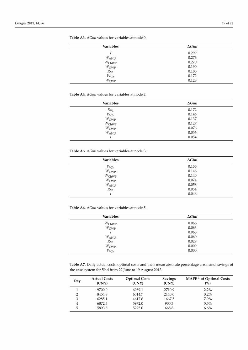
This study employs the operation data of 1416 periods from 22 June to 19 August 2013to model the decision tree using the CART algorithm to recognize the operating modes.The established decision tree is shown in Figure 3. In the modeling process, the ∆Ginivalues of the variables for each node containing multiple operating modes (also known asthe internal node, i.e., nodes 0, 2, 3, and 5) are shown in Tables A3–A6 of Appendix A.
Figure 3. Decision-tree classification model for recognizing operation modes.
Energies 2021, 14, 86 13 of 22
Among the four internal nodes of 0, 2, 3, and 5, in node 2, RV1 = 97 is determined as thesplitting criterion based on the monitoring data for the opening of V1 (97.28 ≤ RV1 ≤ 97.89in the “on” state, while the maximum value of 61.20 in the “modulate” state). Meanwhile,the other three nodes use the theoretical values of the variable in the correspondingclassifications to establish the criterion. This, in turn, enables the checking for anomalies inthe actual operational data (e.g., the over-running in Section 3.4).
3.2. Regression Results of ME
Following the fitting method in Section 2.6, the fitting results and valid internals ofenergy consumption and flow rate for the nine pumps in the case system are presented inTable 4.
Table 4. Fitting results of energy-consumption and flow rate of the nine pumps in the case system.
Items Fitting Model Estimates of Coefficient Range of Value
Considering Ch-1 (Chiller #1) in the cooling mode (i.e., corresponding to operatingmodes M2 and M4) as an example, the fitting results of energy consumption based onEquation (3) in Section 2.6 are listed in Table 5. Similar results for the ice-building mode(i.e., corresponding to operating mode M1) of Ch-1 and two modes of Ch-2 (Chiller #2) arenot listed because of space limitations.
Table 5. Fitting results of the energy-consumption for chiller 1(Ch-1) in cooling mode.
Coefficient Each Item of the Polynomial Coefficient Estimate Standard Error
For the PSO algorithm, the values of C1, C2, and w may influence the computationalresults [24]. After loading the data for 59 d from the case system into the algorithmdescribed in Section 2.8, better results can be obtained by multiple trial calculations todetermine the parameters C1 = 2, C2 = 2, and w = 0.6. Table 6 shows the average results for10 consecutive calculations at various iteration sizes. Moreover, the single minimum energycost appears in the calculation process with an iteration scale of No. 6, 307,213.5 CNY.It saves 97,156.0 CNY or 24.03% compared to the actual energy cost of 404,369.5 CNY.The comparison between the two scenarios for each day is shown in Figure 4. The specificdata in Figure 4 are listed in Table A7 in Appendix A, and the mean absolute percentageerror (MAPE) of the optimal costs for each day are reported simultaneously in the table.
Table 6. Average results of various iteration sizes.
No. Particle Quantity Steps of Iterations Time Cost (s) Average Result (CNY)
Figure 4. Comparison between the daily actual costs, optimal costs, and savings of the case systemfor 59 d from 22 June to 19 August 2013.
When combining these results, the following conclusions can be drawn about thesystematic approach of this study:
First, in Figure 4, the case system has different levels of energy-saving potential foreach day, indicating and validating the effectiveness of the optimization algorithm in thisstudy. Second, it is evident from the results in Table 6 that the difference between themaximum and minimum values of the average results of eight types of iteration sizesis only 5.6%. This is in combination with the MAPE results of the optimization costs inTable A7 (ranging from 2.2% to 11.1%, with an average of 6.2%), demonstrating the highstability of the optimization algorithm. Third, owing to the complexity of the case systemmodel and the numerous constraints, the process of the savings potential calculation istime-consuming. The algorithm needs to be further improved to address this shortcoming.
Energies 2021, 14, 86 15 of 22
3.4. Discussion about Selection of Models
Considering that the main purpose of this paper was to implement and validate thesystematic approach by applying it to a real-life system, we did not focus on the specificmodels and algorithms used for the case study. It is noteworthy that the specific modelsapplied in this study exhibit considerable necessity and superiority.
In terms of the model used for recognition of system-operation mode, the CARTalgorithm was chosen to construct the decision tree model in this paper. Relative to otherclustering models, the CART has better interactivity so that the background knowledge forthe decision tree can be incorporated. [20] Furthermore, the actual and theoretical valuesof the relevant variables during system operation were both considered in the splittingcriterion. For example, when V1 is in the “on” state, the actual value of RV1 was between97.28 and 97.89, instead of the theoretical value of 100. Considering the real-life operation,this study determined RV1 = 97 as the splitting criterion of node 2. As for the splittingcriterion of equipment energy consumption, this paper took the theoretical values in Table 3.The model was thus built not only to identify the system-operation mode but also eligibleto check for anomalies in the actual operating data. For instance, according to the model(Figure 3), the moment in Table A2 in Appendix A at 09:00 on 18 August 2013 was identifiedas M3 (the relevant parameters for this moment were: i = 9, RV1 = 1.44, WCh = 0, WChWP =7.9). Therefore, based on the rules shown in Table 3, the condensing water pumps shouldbe in a shutdown state, and WCWP should be 0, while the actual value of WCWP was 1.1.It indicates an abnormal running of the pumps, where the energy-saving potential exists.After statistics, the energy costs caused by over-running account for 3.8% of the total costs.The detection of such anomalies would further demonstrate the superiority of the modelused in this study.
With respect to the optimization model, indeed, many optimization algorithms canbe applied to the potential analysis session. In addition to the PSO method, we alsoexamined the performance of other algorithms, including genetic algorithm (GA) and antcolony optimization (ACO). As seen in Figure A1, PSO had better optimization resultsat the same time-consuming level (~1000 s) relative to GA and ACO—15% and 8% moreenergy-saving potential were obtained by PSO than GA and ACO, respectively. We alsoacknowledge that comparative studies of the different optimization algorithms in termsof feasibility and consumption need to be undertaken in the future to obtain the greatestpossible energy–cost-saving potential.
3.5. Advantages of the Systematic Method
The detailed case study verifies and demonstrates the feasibility, effectiveness, and sta-bility of the systematic approach. In addition, the proposed method exhibits obviousadvantages over the conventional OTI method. Owing to the elimination of a significantamount of on-site work, including communication with users and system testing in the OTImethod, the proposed method can reduce the time consumed for energy-saving potentialanalysis of complex systems from weeks or months to days, or even shorter. Likewise,the proposed method consumes much fewer human resources than the conventionalmethod. In addition, the conventional OTI method focuses on more specific problems.Hence, the follow-up measurements and analyses are mainly focused on achieving the localoptimization of specific equipment in the system. The results may work well for the specificequipment, but not necessarily for the system. On the contrary, the proposed method ismore comprehensive, considers the extensive constraints in the actual operation of thesystem, and utilizes artificial intelligence algorithms to achieve the global optimization ofthe entire system. Furthermore, the systematic method allows for the modular and batchprocessing of data, as well as remote analysis and online diagnosis, thus providing betterversatility and scalability.
Energies 2021, 14, 86 16 of 22
3.6. Limitations and Future Outlook
The limitations of the proposed systematic method and the case study need to bealleviated in future work and are listed as follows:
• As previously stated, owing to the lack of sufficient data on cooling towers andterminal AHUs for analysis, the case study could not optimize the energy costssimultaneously in the final optimization. However, this issue does not affect thescientific and systematic nature of the study;
• The final optimization of the method pertained to the whole system rather than theindividual devices. This limits the optimization solutions based on the performanceof individual devices.
• It is crucial to achieve the energy-saving operation of the air-conditioning systemthrough the improvement of the control strategy, to attain or approach the result ofenergy-saving potential calculation. Obtaining a set of analysis and operation methodscombining potential calculation and optimization control is a practical problem thatneeds further attention;
• In the research process of diagnostic methods and the employment of these methods todiagnose real air-conditioning systems, the visualization and professional interactionof information and data cannot only improve work efficiency but also have a significantimpact on the understanding and application of the relevant results. This is a potentialdirection for future research.
4. Conclusions
The paper presents a detailed case study of an ice-storage air-conditioning systemusing the method based on data-mining proposed in the companion paper. The raw datawere preprocessed prior to recognizing the constant- and variable-speed devices in thesystem. The classification- and regression-tree algorithms were used to identify the oper-ating modes of the system. The regression models between the energy-consumption andoperating-state parameters of the nine pumps and two chillers were fitted. Subsequently,the constraints related to the system operation were summarized. From the results, the par-ticle swarm optimization method was applied to obtain the benchmark energy cost andthe consequent cost-saving potential. The cost-saving potential for the chiller plant roomduring the 59 d of investigation reached as high as 24.03%. The case study validates anddemonstrates the feasibility, effectiveness, and stability of the systematic approach.
Compared with conventional methods, which take weeks or even longer for energy-saving potential analyses, the proposed method takes only a few days or less. This en-hanced speed indicates that the new systematic approach effectively identifies systemdefaults and reduces the time spent on troubleshooting. The proposed method providesa new approach for studying actual operation data, which is significant in enhancing theenergy efficiency of air-conditioning systems. Future research is warranted to developcorresponding control strategies based on the potential analysis results, investigate betteroptimization algorithms, and visualize the analysis process.
Author Contributions: Conceptualization and project administration, R.M.; methodology and dataanalysis, R.M. and S.Y.; academic guidance, resources, and supervision, X.W., X.-C.W., N.Y., X.Y.,and M.S.; writing—original draft, R.M., and S.Y.; writing—review and editing, X.W., X.-C.W., M.S.,X.Y., N.Y., and S.Y.; funding acquisition, X.Y., M.S., and R.M. All authors have read and agreed to thepublished version of the manuscript.
Funding: This study was supported by the State Key Laboratory of Air-conditioning Equipmentand System Energy Conservation (Grant No. ACSKL2018KT1201), National Science and TechnologyPillar Program during the Thirteenth Five-year Plan Period (Grant No. 2018YFD1100702), and BeijingScience and Technology Program (Grant No. Z181100005418005).
Institutional Review Board Statement: Not applicable.
Informed Consent Statement: Not applicable.
Energies 2021, 14, 86 17 of 22
Data Availability Statement: Data was obtained from Energy Solution Development (Shenzhen)Company Limited, which is not allowed to share data other than that already disclosed herein.
Acknowledgments: The authors would like to thank Yuyang Feng of Energy Solution Development(Shenzhen) Company Limited for providing the case data for this study.
Conflicts of Interest: The authors declare no conflict of interest.
AbbreviationsACO Ant colony optimizationAHU Air handling unitANN Artificial neural networkCART Classification and regression treesCh ChillerChWP Chilled-water pumpChPR Chiller plant roomCWP Condensing-water pumpGA Genetic algorithmGWP Glycol water pumpHVAC Heating, ventilating and air conditioningIST Ice storage tankMAPE Mean absolute percentage errorNN Neural networkOTI Observation/question, test/calculation, and identification/resolutionPHEX Plate heat exchangerPSO Particle swarm optimizationRSM Response surface methodologySAX Symbolic aggregate approximationSI Système internationalSVM Support vector machineUSRT US refrigeration ton
Appendix A
Table A1. Electricity tariffs (ei) at different time intervals of the day.
Table A7. Daily actual costs, optimal costs and their mean absolute percentage error, and savings ofthe case system for 59 d from 22 June to 19 August 2013.
Figure A1. Comparison of optimal costs of the case system calculated by three algorithms (particleswarm optimization (PSO), genetic algorithm (GA) and ant colony optimization (ACO)) for 59 dfrom 22 June to 19 August 2013.
References1. Ma, R.; Wang, X.; Wang, X.-C.; Shan, M.; Yang, X.; Yu, N.; Yang, S. Systematic method for energy saving potential calculation of
air conditioning systems via data mining. Part I: Methodology. Energies 2020, 14, 81. [CrossRef]2. Zhao, Y.; Zhang, C.; Zhang, Y.; Wang, Z.; Li, J. A review of data mining technologies in building energy systems: Load prediction,
pattern identification, fault detection and diagnosis. Energy Built Environ. 2020, 1, 149–164. [CrossRef]3. Zhou, Q.; Wang, S.; Xiao, F. A novel strategy for the fault detection and diagnosis of centrifugal chiller systems. HVAC R Res.
2009, 15, 57–75. [CrossRef]4. Han, H.; Gu, B.; Kang, J.; Li, Z.R. Study on a hybrid SVM model for chiller FDD applications. Appl. Therm. Eng. 2011, 31, 582–592.
[CrossRef]5. Van Every, P.M.; Rodriguez, M.; Jones, C.B.; Mammoli, A.A.; Martínez-Ramón, M. Advanced detection of HVAC faults using
unsupervised SVM novelty detection and Gaussian process models. Energy Build. 2017, 149, 216–224. [CrossRef]6. Yan, R.; Ma, Z.; Zhao, Y.; Kokogiannakis, G. A decision tree based data-driven diagnostic strategy for air handling units. Energy
Build. 2016, 133, 37–45. [CrossRef]7. Lee, W.Y.; Park, C.; House, J.M.; Kelly, G.E. Fault diagnosis of an air-handling unit using artificial neural networks. ASHRAE
Trans. 1996, 102, 540–549.8. Magoulès, F.; Zhao, H.; Elizondo, D. Development of an RDP neural network for building energy consumption fault detection
and diagnosis. Energy Build. 2013, 62, 133–138. [CrossRef]9. Patnaik, D.; Marwah, M.; Sharma, R.; Ramakrishnan, N. Sustainable operation and management of data center chillers using
temporal data mining. In Proceedings of the 15th ACM SIGKDD International Conference on Knowledge Discovery and DataMining, Paris, France, 28 June–1 July 2009; pp. 1305–1314.
10. Chen, Y.; Wen, J. Whole building system fault detection based on weather pattern matching and PCA method. In Proceedings of the2017 3rd IEEE International Conference on Control Science and Systems Engineering (ICCSSE), Beijing, China, 17–19 August 2017;pp. 728–732.
11. Li, G.; Hu, Y.; Chen, H.; Li, H.; Hu, M.; Guo, Y.; Liu, J.; Sun, S.; Sun, M. Data partitioning and association mining for identifyingVRF energy consumption patterns under various part loads and refrigerant charge conditions. Appl. Energy 2017, 185, 846–861.[CrossRef]
12. Li, Z.X.; Renault, F.L.; Gómez, A.O.C.; Sarafraz, M.M.; Khan, H.; Safaei, M.R.; Filho, E.P.B. Nanofluids as secondary fluid inthe refrigeration system: Experimental data, regression, ANFIS, and NN modeling. Int. J. Heat Mass Transf. 2019, 144, 118635.[CrossRef]
13. Sarafraz, M.M.; Tlili, I.; Tian, Z.; Bakouri, M.; Safaei, M.R. Smart optimization of a thermosyphon heat pipe for an evacuated tubesolar collector using response surface methodology (RSM). Phys. A Stat. Mech. its Appl. 2019, 534, 122146. [CrossRef]
14. Sarafraz, M.M.; Safaei, M.R.; Goodarzi, M.; Arjomandi, M. Experimental investigation and performance optimisation of a catalyticreforming micro-reactor using response surface methodology. Energy Convers. Manag. 2019, 199, 111983. [CrossRef]
15. Rosas-Flores, J.A.; Rosas-Flores, D. Potential energy savings and mitigation of emissions by insulation for residential buildings inMexico. Energy Build. 2020, 209, 109698. [CrossRef]
16. Zeng, Y.; Zhang, Z.; Kusiak, A. Predictive modeling and optimization of a multi-zone HVAC system with data mining and fireflyalgorithms. Energy 2015, 86, 393–402. [CrossRef]
17. Kwame, A.B.O.; Troy, N.V.; Hamidreza, N. A Multi-Facet Retrofit Approach to Improve Energy Efficiency of Existing Class ofSingle-Family Residential Buildings in Hot-Humid Climate Zones. Energies 2020, 13, 1178. [CrossRef]
18. Tian, Z.; Si, B.; Wu, Y.; Zhou, X.; Shi, X. Multi-objective optimization model predictive dispatch precooling and ceiling fans inoffice buildings under different summer weather conditions. Build. Simul. 2019, 12, 999–1012. [CrossRef]
19. Ma, R.; Wang, X.; Shan, M.; Yu, N.; Yang, S. Recognition of variable-speed equipment in an air-conditioning system usingnumerical analysis of energy-consumption data. Energies 2020, 13, 4975. [CrossRef]
20. Han, J.; Kamber, M.; Pei, J. Data Mining: Concepts and Techniques, 3rd ed.; Elsevier Inc.: Waltham, MA, USA, 2012;ISBN 9780123814791.
21. Zhang, G.; Chen, L. Opmization of energy consumption in chilled plant. Fluid Mach. 2012, 40, 75–80.22. Ma, R. The Study of Energy Efficiency Diagnosis Methodology for Air-Conditioning Systems with the Actual Operating Data.
Ph.D. Thesis, Southwest Jiaotong University, Chengdu, China, 2014.23. Kennedy, J.; Eberhart, R. Particle Swarm Optimization. In Proceedings of the IEEE International Conference on Neural Networks,
Perth, Australia, 27 November–1 December 1995; Volume 4, pp. 1942–1948.24. Ma, R.-J.; Yu, N.-Y.; Hu, J.-Y. Application of particle swarm optimization algorithm in the heating system planning problem. Sci.