Systems with inheritance: dynamics ofdistributions with conservation of support,

natural selection and finite-dimensionalasymptotics

Alexander N. Gorban∗

ETH-Zentrum, Department of Materials, Institute of Polymers,Sonneggstr. 3, ML J19, CH-8092 Zurich, Switzerland;

Institute of Computational Modeling SB RAS,Akademgorodok, Krasnoyarsk 660036, Russia

Abstract

If we find a representation of an infinite-dimensional dynamical system as a non-linear kinetic system with conservation of supports of distributions, then (after someadditional technical steps) we can state that the asymptotics is finite-dimensional.This conservation of support has a quasi-biological interpretation, inheritance (if agene was not presented initially in a isolated population without mutations, thenit cannot appear at later time). These quasi-biological models can describe vari-ous physical, chemical, and, of course, biological systems. The finite-dimensionalasymptotic demonstrates effects of “natural” selection. The estimations of asymp-totic dimension are presented. The support of an individual limit distribution isalmost always small. But the union of such supports can be the whole space evenfor one solution. Possible are such situations: a solution is a finite set of narrowpeaks getting in time more and more narrow, moving slower and slower. It is pos-sible that these peaks do not tend to fixed positions, rather they continue moving,and the path covered tends to infinity at t →∞. The drift equations for peaks mo-tion are obtained. Various types of stability are studied. In example, models of celldivision self-synchronization are studied. The appropriate construction of notionof typicalness in infinite-dimensional spaces is discussed, and the “completely thin”sets are introduced.

1 Introduction: Unusual conservation law

In the 1970th-1980th years, theoretical studies developed one more “common” field be-longing simultaneously to physics, biology and mathematics. For physics it is (so far)a part of the theory of approximations of a special kind, demonstrating, in particular,

∗agorban@mat.ethz.ch

1

interesting mechanisms of discreteness in the course of evolution of distributions with ini-tially smooth densities. But what for physics is merely a convenient approximation, is afundamental law in biology (inheritance), whose consequences comprehended informally(selection theory [1, 2, 3, 4, 8, 9, 7])1 permeate most of the sections of this science.

Consider a community of animals. Let it be biologically isolated. Mutations can beneglected in the first approximation. In this case new genes do not emerge.

And here is an example is from physics. Let waves with wave vectors k be excited insome system. Denote K a set of wave vectors k of excited waves. Let the waves interactiondo not lead to generation of waves with new k /∈ K. Such an approximation is applicableto a variety of situations. For the wave turbulence it was described in detail in [10, 11].

What is common in these examples is the evolution of a distribution with a supportnot increasing in time.

What does not increase must, as a rule, decrease, if the decrease is not prohibited. Thisnaive thesis can be converted into rigorous theorems for the case under consideration [7].The support is proved to decrease in the limit t →∞, if it was sufficiently large initially.Considered usually are such system, for which at finite times the distributions supportconserves and decrease only in the limit t → ∞. Conservation of the support usuallyresults in the following effect: dynamics of initially infinite-dimensional system at t →∞can be described by finite-dimensional systems.

The simplest and most common in applications class of equations for which the dis-tributions support does not grow in time, is constructed as follows. To each distributionµ is assigned a function kµ by which the distribution can be multiplied. Written down isequation

dµ

dt= kµ × µ. (1)

The multiplier kµ is called a reproduction coefficient. The right-hand side is the productof the function kµ with the distribution µ, hence dµ/dt should be zero where µ is equalto zero, therefore the support of µ is conserved in time (over the finite times).

Let us remind the definition of the support. Each distribution on a compact space Xis a continuous linear functional on the space of continuous functions C(X)2. The spaceC(X) is the Banach space endowed with the norm

‖f‖ = maxx∈X

|f(x)|. (2)

Usually, when X is a bounded closed subset of a finite-dimensional space, we representthis functional as the integral

µ[f ] =

∫µ(x)f(x) dx,

where µ(x) is the (generalized) density function of the distribution µ. The support ofµ, suppµ, is the smallest closed subset of X with the following property: if f(x) = 0 onsuppµ, then µ[f ] = 0, i.e. µ(x) = 0 outside suppµ.

1We do not try to review the scientific literature about the evolution, and mention here only thereferences that are especially important for our understanding of the selection theory and applications.

2We follow the Bourbaki approach [18]: a measure is a continuous functional, an integral. The book[18] contains all the necessary notions and theorems (and much more material than we need here).

2

Strictly speaking, the space on which µ is defined and the distribution class it belongsto, should be specified. One should also specify are properties of the mapping µ 7→ kµ

and answer the question of existence and uniqueness of solutions of (1) under given initialconditions. In specific situations the answers to these questions are not difficult.

Let us start with the simplest example

∂µ(x, t)

∂t=

[f0(x)−

∫ b

a

f1(x)µ(x, t) dx

]µ(x, t), (3)

where the functions f0(x)andf1(x) are positive and continuous on the closed segment [a, b].Let the function f0(x) reaches the global maximum on the segment [a, b] at a single pointx0. If x0 ∈ suppµ(x, 0), then

µ(x, t) → f0(x0)

f1(x0)δ(x− x0), when t →∞, (4)

where δ(x− x0) is the δ-function.We use in the space of measures the weak convergence, i.e. the convergence of averages:

µi → µ∗ if and only if

∫µiϕ(x) dx →

∫µ∗ϕ(x) dx (5)

for all continuous functions ϕ(x). This weak convergence of measures generates the weaktopology on the space of measures (the weak topology of conjugated space).

If f0(x) has several global maxima, then the right-hand side of (4) can be a sum of afinite number of δ-functions. Here a natural question arises: is it worth to pay attentionto such a possibility? Should not we deem improbable for f0(x) to have more than oneglobal maximum? Indeed, such a case seems to be very unlikely to occur. More detailsabout this are given below.

Equations in the form (1) allow the following biological interpretation: µ is the dis-tribution of the number (or of a biomass, or of another extensive variable) over inheritedunits: species, varieties, supergenes, genes. Whatever is considered as the inherited unitdepends on the context, on a specific problem. The value of kµ(x) is the reproductioncoefficient of the inherited unit x under given conditions. The notion of “given conditions”includes the distribution µ, the reproduction coefficient depends on µ. Equation (3) canbe interpreted as follows: f0(x) is the specific birth-rate of the inherited unit x (below, forthe sake of definiteness, x is a variety, following the spirit of the famous Darwin’s book[1]), the death rate for the representatives of all inherited units (varieties) is determined

by one common factor depending on the density∫ b

af1(x)µ(x, t) dx; f1(x) is the individual

contribution of the variety x into this death-rate.On the other hand, for systems of waves with a parametric interaction, kµ(x) can be

the amplification (decay) rate of the wave with the wave vector x.The first step in the routine of a dynamical system investigation is the question about

fixed points and their stability. And the first observation concerning the system (1) is thatasymptotically stable can be only the steady-state distributions, whose support is discrete(i.e. the sums of δ-functions). This can be proved for all the consistent formalizations,and can be understood as follows.

Let the “total amount” (integral of |µ| over U) be less than ε > 0 but not equal to zeroin some domain U . Substitute distribution µ by zero on U , the rest remains as it is. It is

3

natural to consider this disturbance of µ as ε-small. However, if the dynamics is describedby (1), there is no way back to the undisturbed distribution, because the support cannotincrease. If the steady state distribution µ∗ is asymptotically stable, then for some ε > 0any ε-small perturbation of µ∗ relaxes back to µ∗. This is possible only in the case iffor any domain U the integral of |µ∗| over U is either 0 or greater than ε. Hence, thisasymptotically stable distribution µ∗ is the sum of the finite number of δ-functions:

µ∗(x) =

q∑i=1

Niδ(x− xi) (6)

with |Ni| > ε for all i.So we have: the support of asymptotically stable distributions for the system (1)

is always discrete. This simple observation has many strong generalizations to generalω-limit points, to equations for vector measures, etc.

Dynamic systems where the phase variable is a distribution µ, and the distributionsupport is the integral of motion, frequently occur both in physics and in biology. Becauseof their attractive properties they are frequently used as approximations: we try to find the“main part” of the system in the form (1), and represent the rest as a small perturbationof the main part.

In biology such an approximation is essentially all the classical genetics, and also theformal contents of the theory of natural selection. The initial diversity is “thinned out”in time, and the limit distribution supports are described by some extremal principles(principles of optimality).

Conservation of the support in equation (1) can be considered as inheritance, and,consequently, we call the system (1) and its nearest generalizations “systems with in-heritance”. Traditional division of the process of transferring biological information intoinheritance and mutations, small in any admissible sense, can be compared to the descrip-tion according to the following pattern: system (1) (or its nearest generalizations) plussmall disturbances. Beyond the limits of such a description, talking about inheritanceloses the conventional sense.

The first study of the dynamics systems with inheritance was due to J.B.S. Haldane.He used the simplest examples, studied steady-state distributions, and obtained the ex-tremal principle for them. His pioneering book “The Causes of Evolution” (1932) [2]gives the clear explanation of the connections between the inheritance (the conservationof distributions support) and the optimality of selected varieties.

Haldane’s work was followed by entirely independent series of works on the S-approximationin the spin wave theory and on the wave turbulence [10, 11, 12], which studied wave con-figurations in the approximation of “inherited” wave vector, and by “Synergetics” [17],where the “natural selections” of modes is one of the basic concepts.

At the same time, a series of works on biological kinetics was done (see, for example, [5,6, 8, 7]). The studies addressed not only steady-states, but also common limit distributions[6, 7] and waves in the space of inherited units [5]. For the steady-states a new type ofstability was described – the stable realizability (see below).

The purpose of this paper is to present general results of the theory of systems withinheritance: optimality principles the for limit distributions, theorems about selection,and estimations of the limit diversity (estimates of number of points in the supportsof the limit distributions), drift effect and drift equations. Some of these result werepublished in preprints in Russian [6] (and, partially, in the Russian book [7]).

4

2 Optimality principle for limit diversity

Description of the limit behavior of a dynamical system does not necessarily reduce toenumerating stable fixed points and limit cycles. The possibility of stochastic oscillationsis common knowledge, while the domains of structurally unstable (non coarse) systemsdiscovered by S. Smale [19]3 have so far not been mastered in applied and natural sciences).

The leading rival to adequately formalize the limit behavior is the concept of the “ω-limit set”. It was discussed in detail in the classical monograph [20]. The fundamentaltextbook on dynamical systems [21] and the introductory review [22] are also available.

If f(t) is the dependence of the position of point in the phase space on time t (i.e.the motion of the dynamical system), then the ω-limit points are such points y, for whichthere exist such sequences of times ti →∞, that f(ti) → y.

The set of all ω-limit points for the given motion f(t) is called the ω-limit set. If,for example, f(t) tends to the equilibrium point y∗ then the corresponding ω-limit setconsists of this equilibrium point. If f(t) is winding onto a closed trajectory (the limitcycle), then the corresponding ω-limit set consists of the points of the, cycle and so on.

General ω-limit sets are not encountered oft in specific situations. This is because ofthe lack of efficient methods to find them in a general situation. Systems with inheritanceis a case, where there are efficient methods to estimate the limit sets from above. This isdone by the optimality principle.

Let µ(t) be a solution of (1). Note that

µ(t) = µ(0) exp

∫ t

0

kµ(τ) dτ. (7)

Here and below we do not display the dependence of distributions µ and of the reproduc-tion coefficients k on x when it is not necessary. Fix the notation for the average value ofkµ(τ) on the segment [0, t]

〈kµ(t)〉t =1

t

∫ t

0

kµ(τ) dτ. (8)

Then the expression (7) can be rewritten as

µ(t) = µ(0) exp(t〈kµ(t)〉t). (9)

If µ∗ is the ω-limit point of the solution µ(t), then there exists such a sequence of timesti → ∞, that µ(ti) → µ∗. Let it be possible to chose a convergent subsequence of thesequence of the average reproduction coefficients 〈kµ(t)〉t, which corresponds to times ti.We denote as k∗ the limit of this subsequence. Then, the following statement is valid: onthe support of µ∗ the function k∗ vanishes and on the support of µ(0) it is non-positive:

k∗(x) = 0 if x ∈ suppµ∗,

k∗(x) ≤ 0 if x ∈ suppµ(0). (10)

3“Structurally stable systems are not dense”. Without exaggeration we can say that so entitled work[19] opened a new era in the understanding of dynamics. Structurally stable (rough) systems are thosewhose phase portraits do not change qualitatively under small perturbations. Smale constructed suchstructurally unstable system that any other system close enough to it is also structurally unstable. Thisresult defeated hopes for a classification if not all, but at least “almost all” dynamical systems. Suchhopes were associated with the success of the classification of two-dimensional dynamical systems, amongwhich structurally stable systems are dense.

5

Taking into account the fact that suppµ∗ ⊆ suppµ(0), we come to the formulation ofthe optimality principle (10): The support of limit distribution consists of points of theglobal maximum of the average reproduction coefficient on the initial distribution support.The corresponding maximum value is zero.

We should also note that not necessarily all points of maximum of k∗ on suppµ(0)belong to suppµ∗, but all points of suppµ∗ are the points of maximum of k∗ on suppµ(0).

If µ(t) tends to the fixed point µ∗, then 〈kµ(t)〉t → kµ∗ as t →∞, and suppµ∗ consistsof the points of the global maximum of the corresponding reproduction coefficient kµ∗ onthe support of µ∗. The corresponding maximum value is zero.

If µ(t) tends to the limit cycle µ∗(t) (µ∗(t+T ) = µ∗(t)), then all the distributions µ∗(t)have the same support. The points of this support are the points of maximum (global,zero) of the averaged over the cycle reproduction coefficient

k∗ = 〈kµ∗(t)〉T =1

T

∫ T

0

kµ∗(τ) dτ, (11)

on the support of µ(0).The supports of the ω-limit distributions are specified by the functions k∗. It is

obvious where to get these functions from for the cases of fixed points and limit cycles.There are at least two questions: what ensures the existence of average reproductioncoefficients at t →∞, and how to use the described extremal principle (and how efficientis it). The latter question is the subject to be considered in the following sections. Inthe situation to follow the answers to these questions have the validity of theorems. LetX be a space on which the distributions are defined. Assume it to be a compact metricspace (for example, a closed bounded subset of Euclidian space). The distribution µ isidentified with the Radon measure, that is the continuous linear functional on the spaceof continuous functions on X, C(X). We use the conventional notation for this linearfunctional as the integral of the function ϕ as

∫ϕ(x)µ(x) dx. Here µ(x) is acting as the

distribution density, although, of course, the arbitrary X has no initial (Lebesgue, forexample) dx.

The sequence of continuous functions ki(x) is considered to be convergent if it convergesuniformly. The sequence of measures µi is called convergent if for any continuous functionϕ(x) the integrals

∫ϕ(x)µi(x) dx converge (weak convergence (5)). The mapping µ 7→ kµ

assigning the reproduction coefficient kµ to the measure µ is assumed to be continuous.And, finally, the space of measures is assumed to have a bounded4 set M which is positivelyinvariant relative to system (1): if µ(0) ∈ M , then µ(t) ∈ M (and is non-trivial). This Mwill serve as the phase space of system (1).

Most of the results about systems with inheritance use the theorem about weakcompactness: The bounded set of measures is precompact with respect to the the weakconvergence (i.e., its closure is compact). Therefore, the set of corresponding reproductioncoefficients kM = {kµ|µ ∈ M} is precompact, the set of averages (8) is precompact,because it is the subset of the closed convex hull conv(kM) of the compact set. Thiscompactness allows us to claim the existence of the average reproduction coefficient k∗ forthe description of the ω-limit distribution µ∗ with the optimality principle (10).

4The set of measures M is bounded, if the sets of integrals {µ[f ]|µ ∈ M, ‖f‖ ≤ 1} is bounded, where‖f‖ is the norm (2).

6

3 How many points

does the limit distribution support hold?

The limit distribution is concentrated in the points of (zero) global maximum of theaverage reproduction coefficient. The average is taken along the solution, but the solutionis not known beforehand. With the convergence towards a fixed point or to a limit cyclethis difficulty can be circumvented. In the general case the extremal principle can beused without knowing the solution, in the following way [7]. Considered is a set of alldependencies µ(t) where µ belongs to the phase space, the bounded set M . The set ofall averages over t is {〈kµ(t)〉t}. Further, taken are all limits of sequences formed by theseaverages – the set of averages is closed. The result is the closed convex hull conv(kM) ofthe compact set kM . This set involves all possible averages (8) and all their limits. Inorder to construct it, the true solution µ(t) is not needed.

The weak optimality principle is expressed as follows. Let µ(t) be a solution of (1) inM , µ∗ is any of its ω-limit distributions. Then in the set conv(kM) there is such a functionk∗ that its maximum value on the support suppµ0 of the initial distribution µ0 equals tozero, and suppµ∗ consists of the points of the global maximum of k∗ on suppµ0 only (10).

Of course, in the set conv(kM) usually there are many functions that are irrelevant tothe time average reproduction coefficients for the given motion µ(t). Therefore, the weakextremal principle is really weak – it gives too many possible supports of µ∗. However,even such a principle can help to obtain useful estimates of the number of points in thesupports of ω-limit distributions.

It is not difficult to suggest systems of the form (1), in which any set can be thelimit distribution support. The simplest example: kµ ≡ 0. Here ω-limit (fixed) is anydistribution. However, almost any arbitrary small perturbation of the system destroysthis pathological property.

In the realistic systems, especially in biology, the coefficients fluctuate and are neverknown exactly. Moreover, the models are in advance known to have a finite error whichcannot be exterminated by the choice of the parameters values. This gives rise to an ideato consider not individual systems (1), but ensembles of similar systems [7].

Having posed the questions of how many points can the support of ω-limit distributionshave, estimate the maximum for each individual system from the ensemble (in its ω-limitdistributions), and then, estimate the minimum of these maxima over the whole ensemble– (the minimax estimation). The latter is motivated by the fact, that if the inheritedunit has gone extinct under some conditions, it will not appear even under the change ofconditions.

Let us consider an ensemble that is simply the ε-neighborhood of the given system(1). The minimax estimates of the number of points in the support of ω-limit distributionare constructed by approximating the dependencies kµ by finite sums

kµ = ϕ0(x) +n∑

i=1

ϕi(x)ψi(µ). (12)

Here ϕi depend on x only, and ψi depend on µ only. Let εn > 0 be the distance fromkµ to the nearest sum (12) (the “distance” is understood in the suitable rigorous sense,which depends on the specific problem). So, we reduced the problem to the estimation ofthe diameters εn > 0 of the set conv(kM).

7

The minimax estimation of the number of points in the limit distributionsupport gives the answer to the question, “How many points does the limit distributionsupport hold”: If ε > εn then, in the ε-vicinity of kµ, the minimum of the maxima of thenumber of points in the ω-limit distribution support does not exceed n.

In order to understand this estimate it is sufficient to consider system (1) with kµ ofthe form (12). The averages (8) for any dependence µ(t) in this case have the form

〈kµ(t)〉t =1

t

∫ t

0

kµ(τ) dτ = ϕ0(x) +n∑

i=1

ϕi(x)ai. (13)

where ai are some numbers. The ensemble of the functions (13) for various ai forms an-dimensional linear manifold. How many of points of the global maximum (equal tozero) could a function of this family have?

Generally speaking, it can have any number of maxima. However, it seems obvious,that “usually” one function has only one point of global maximum, while it is “improb-able” the maximum value is zero. At least, with an arbitrary small perturbation of thegiven function, we can achieve for the point of the global maximum to be unique and themaximum value be non-zero.

In a one-parametric family of functions there may occur zero value of the global max-imum, which cannot be eliminated by a small perturbation, and individual functions ofthe family may have two global maxima.

In the general case we can state, that “usually” each function of the n-parametricfamily (13) can have not more than n− 1 points of the zero global maximum (of course,there may be less, and for the majority of functions of the family the global maximum,as a rule, is not equal to zero at all). What “usually” means here requires a specialexplanation given in the next section.

In application kµ is often represented by an integral operator, linear or nonlinear. Inthis case the form (12) corresponds to the kernels of integral operators, represented in aform of the sums of functions’ products. For example, the reproduction coefficient of thefollowing form

kµ = ϕ0(x) +

∫K(x, y)µ(y) dy,

where K(x, y) =n∑

i=1

ϕi(x)gi(y), (14)

has also the form (12) with ψi(µ) =∫

gi(y)µ(y) dy.The linear reproduction coefficients occur in applications rather frequently. For them

the problem of the minimax estimation of the number of points in the ω-limit distributionsupport is reduced to the question of the accuracy of approximation of the linear integraloperator by the sums of kernels-products (14).

4 Selection efficiency

The first application of the extremal principle for the ω-limit sets is the theorem of theselection efficiency. The dynamics of a system with inheritance indeed leads in the limitt →∞ to a selection. In the typical situation, a diversity in the limit t →∞ becomes less

8

than the initial diversity. There is an efficient selection for the “best”. The basic effectsof selection are formulated below.

Theorem of selection efficiency.

1. Almost always the support of any ω-limit distribution is nowhere dense in X (andit has the Lebesgue measure zero for Euclidean space).

2. Let εn > 0, εn → 0 be an arbitrary chosen sequence. The following statementis almost always true for system (1). Let the support of the initial distributionbe the whole X. Then the support of any ω-limit distribution µ∗ is almost finite.This means that it is approximated by finite sets faster than εn → 0: there is anumber N , such that for n > N there exists a finite set Sn of n elements such thatdist(Sn, suppµ∗) < εn, where dist is the Hausdorff distance between closed subsets ofX:

dist(A,B) = max{supx∈A

infx∈B

ρ(x, y), supx∈B

infx∈A

ρ(x, y)}, (15)

where ρ(x, y) is the distance between points.

3. In the previous statement for any chosen sequence εn > 0, εn → 0, almost allsystems (1) have ω-limit distributions with supports that can be approximated byfinite sets faster than εn → 0. The order is important: “for any sequence almost allsystems...” But if we use only the recursive (algorithmic) analogue of sequences, thenwe can easily prove the statement with the reverse order: “almost all systems forany sequence...” This is possible because the set of all recursive enumerable countablesets is also countable and not continuum. This observation is very important foralgorithmic foundations of probability theory [23]. Let L be a set of all sequencesof real numbers εn > 0, εn → 0 with the property: for each {εn} ∈ L the rationalsubgraph {(n, r) : εn > r ∈ Q} is recursively enumerable. For almost all systems(1) and any {εn} ∈ L the support of any ω-limit distribution µ∗ is approximated byfinite sets faster than εn → 0.

These properties hold for the continuous reproduction coefficients. It is well-known,that it is dangerous to rely on the genericity among continuous functions. For example,almost all continuous functions are nowhere differentiable. But the properties 1 and 2hold also for the smooth reproduction coefficients on the manifolds and sometimes allow toreplace the “almost finiteness” by simply finiteness. In order to appreciate this theorem,note that:

1. Support of an arbitrary ω-limit distribution µ∗ consist of points of global maximumof the average reproduction coefficient on a support of the initial distribution. Thecorresponding maximum value is zero.

2. Almost always a function has only one point of global maximum, and correspondingmaximum value is not 0.

3. In a one-parametric family of functions almost always there may occur zero valuesof the global maximum (at one point), which cannot be eliminated by a smallperturbation, and individual functions of the family may stably have two globalmaximum points.

9

4. For a generic n-parameter family of functions, there may exist stably a functionwith n− 1 points of global maximum and with zero value of this maximum.

5. Our phase space M is compact. The set of corresponding reproduction coefficientskM in C(X) for the given map µ → kµ is compact too. The average reproductioncoefficients belong to the closed convex hull of this set conv(kM). And it is compacttoo.

6. A compact set in a Banach space can be approximated by its projection on anappropriate finite-dimensional linear manifold with an arbitrary accuracy. Almostalways the function on such a manifold may have only n−1 points of global maximumwith zero value, where n is the dimension of the manifold.

The rest of the proof is purely technical. The easiest demonstration of the “natural”character of these properties is the demonstration of instability of exclusions: If, forexample, a function has several points of global maxima then with an arbitrary smallperturbation (for all usually used norms) it can be transformed into a function with theunique point of global maximum. However “stable” does not always mean “dense”. Inwhat sense the discussed properties of the system (1) are usually valid? “Almost always”,“typically”, “generically” a function has only one point of global maximum. This sentenceshould be given an rigorous meaning. Formally it is not difficult, but haste is dangerouswhen defining “genericity”.

Here are some examples of correct but useless statements about “generic” proper-ties of function: Almost every continuous function is not differentiable; Almost everyC1 -function is not convex. Their meaning for applications is most probably this: thegenericity used above for continuous functions or for C1 -function is irrelevant to thesubject.

Most frequently the motivation for definitions of genericity is found in such a situation:given n equations with m unknowns, what can we say about the solutions? The answeris: in a typical situation, if there are more equations, than the unknowns (n > m), thereare no solutions at all, but if n ≤ m (n is less or equal to m), then, either there is a(m− n)-parametric family of solutions, or there are no solutions.

The best known example of using this reasoning is the Gibbs phase rule in classicalchemical thermodynamics. It limits the number of co-existing phases. There exists awell-known example of such reasoning in mathematical biophysics too. Let us consider amedium where n species coexist. The medium is assumed to be described by m parame-ters. In the simplest case, the medium is a well-mixed solution of m substances. Let theorganisms interact through the medium, changing its parameters – concentrations of msubstances. Then, in a steady state, for each of the coexisting species we have an equationwith respect to the state of the medium. So, the number of such species cannot exceedthe number of parameters of the medium. In a typical situation, in the m-parametricmedium in a steady state there can exist not more than m species. This is the Gauseconcurrent exclusion principle [24]. This fact allows numerous generalizations. Theoremof the natural selection efficiency may be considered as its generalization too.

Analogous assertion for a non-steady state coexistence of species in the case of equa-tions (11) is not true. It is not difficult to give an example of stable coexistence underoscillating conditions of n species in the m-parametric medium at n > m. But, if kµ

are linear functions of µ, then for non-stable conditions we have the concurrent exclusion

10

principle, too. In that case, the average in time of reproduction coefficient kµ(t) is thereproduction coefficient for the average µ(t) because of linearity. Therefore, the equationfor the average reproduction coefficient,

k∗(x) = 0 for x ∈ suppµ∗, (16)

transforms into the following equation for the reproduction coefficient of the averagedistribution

k∗(〈µ〉) = 0 for x ∈ suppµ∗ (17)

(the Volterra averaging principle [25]). This system has as many linear equations as ithas coexisting species. The averages can be non-unique. Then all of them satisfy thissystem, and we obtain the non-stationary Gause principle. And again, it is valid “almostalways”.

Formally, various definitions of genericity are constructed as follows. All systems (orcases, or situations and so on) under consideration are somehow parameterized – by setsof vectors, functions, matrices etc. Thus, the “space of systems” Q can be described.Then the “thin sets” are introduced into Q, i.e. the sets, which we shall later neglect.The union of a finite or countable number of thin sets, as well as the intersection of anynumber of them should be thin again, while the whole Q is not thin. There are twotraditional ways to determine thinness.

1. A set is considered thin when it has measure zero. This is good for a finite-dimensional case, when there is the standard Lebesgue measure – the length, thearea, the volume.

2. But most frequently we deal with the functional parameters. In that case it iscommon to restore to the second definition, according to which the sets of firstcategory are negligible. The construction begins with nowhere dense sets. The setY is nowhere dense in Q, if in any nonempty open set V ⊂ Q (for example, in aball) there exists a nonempty open subset W ⊂ V (for example, a ball), which doesnot intersect with Y . Roughly speaking, Y is “full of holes” – in any neighborhoodof any point of the set Y there is an open hole. Countable union of nowhere densesets is called the set of the first category. The second usual way is to define thinsets as the sets of the first category.

But even the real line R can be divided into two sets, one of which has zero measure,the other is of the first category. The genericity in the sense of measure and the genericityin the sense of category considerably differ in the applications where both of these conceptscan be used. The conflict between the two main views on genericity stimulated efforts toinvent new and stronger approaches.

In Theorem of selection efficiency a very strong genericity was used. Systems (1)were parameterized by continuous maps µ 7→ kµ. Denote by Q the space of these mapsM → C(X) with the topology of uniform convergence on M . So, it is a Banach space.We shall call the set Y in the Banach space Q completely thin, if for any compact set Kin Q and arbitrary positive ε > 0 there exists a vector q ∈ Q, such that ‖q‖ < ε andK + q does not intersect Y . So, a set, which can be moved out of intersection with anycompact by an arbitrary small translation, is completely negligible. In a finite-dimensionalspace there is only one such set – the empty one. In an infinite-dimensional Banach

11

space compacts and closed subspaces with infinite codimension provide us examples ofcompletely negligible sets. In Theorem of selection efficiency “usually” means “the set ofexceptions is completely thin”.

5 Gromov’s interpretation of selection theorems

In his talk [26], M. Gromov offered a geometric interpretation of the selection theorems.Let us consider dynamical systems in the standard m-simplex σm in m + 1-dimensionalspace Rm+1:

σm = {x ∈ Rm+1|xi ≥ 0,m+1∑i=1

xi = 1}.

We assume that simplex σm is positively invariant with respect to these dynamical sys-tems: if the motion starts in σm at some time t0 then it remains in σm for t > t0. Let usconsider the motions that start in the simplex σm at t = 0 and are defined for t > 0.

For large m, almost all volume of the simplex σm is concentrated in a small neighbor-hood of the center of σm, near the point c =

(1m

, 1m

, . . . , 1m

). Hence, one can expect that a

typical motion of a general dynamical system in σm for sufficiently large m spends almostall the time in a small neighborhood of c.

Let us consider dynamical systems with an additional property (“inheritance”): allthe faces of the simplex σm are also positively invariant with respect to the systems withinheritance. It means that if some xi = 0 initially at the time t = 0 then xi = 0 for t > 0for all motions in σm. The essence of selection theorems is as follows: a typical motionof a typical dynamical system with inheritance spends almost all the time in a smallneighborhood of low-dimensional faces, even if it starts near the center of the simplex.

Let us denote by ∂rσm the union of all r-dimensional faces of σm. Due to the selectiontheorems, a typical motion of a typical dynamical system with inheritance spends almostall time in a small neighborhood of ∂rσm with r ¿ m. It should not obligatory residenear just one face from ∂rσm, but can travel in neighborhood of different faces from ∂rσm

(the drift effect). The minimax estimation of the number of points in ω-limit distributionsthrough the diameters εn > 0 of the set conv(kM) is the estimation of r.

6 Drift equations

To this end, we talked about the support of an individual ω-limit distribution. Almostalways it is small. But this does not mean, that the union of these supports is small evenfor one solution µ(t). It is possible that a solution is a finite set of narrow peaks getting intime more and more narrow, moving slower and slower, but not tending to fixed positions,rather continuing to move along its trajectory, and the path covered tends to infinity ast →∞.

This effect was not discovered for a long time because the slowing down of the peakswas thought as their tendency to fixed positions. There are other difficulties relatedto the typical properties of continuous functions, which are not typical for the smoothones. Let us illustrate them for the distributions over a straight line segment. Add tothe reproduction coefficients kµ the sum of small and narrow peaks located on a straightline distant from each other much more than the peak width (although it is ε-small).

12

However small is chosen the peak’s height, one can choose their width and frequency onthe straight line in such a way that from any initial distribution µ0 whose support is thewhole segment, at t → ∞ we obtain ω-limit distributions, concentrated at the points ofmaximum of the added peaks.

Such a model perturbation is small in the space of continuous functions. Therefore, itcan be put as follows: by small continuous perturbation the limit behavior of system (1)can be reduced onto a ε-net for sufficiently small ε. But this can not be done with the smallsmooth perturbations (with small values of the first and the second derivatives) in thegeneral case. The discreteness of the net, onto which the limit behavior is reduced by smallcontinuous perturbations, differs from the discreteness of the support of the individualω-limit distribution. For an individual distribution the number of points is estimated,roughly speaking, by the number of essential parameters (12), while for the conjunctionof limit supports – by the number of stages in approximation of kµ by piece-wise constantfunctions.

Thus, in a typical case the dynamics of systems (1) with smooth reproduction coeffi-cients transforms a smooth initial distributions into the ensemble of narrow peaks. Thepeaks become more narrow, their motion slows down, but not always they tend to fixedpositions.

The equations of motion for these peaks can be obtained in the following way [7].Let X be a domain in the n-dimensional real space, and the initial distributions µ0 beassumed to have smooth density. Then, after sufficiently large time t, the position ofdistribution peaks are the points of the average reproduction coefficient maximum 〈kµ〉t(8) to any accuracy set in advance. Let these points of maximum be xα, and

qαij = −t

∂2〈kµ〉t∂xi∂xj

∣∣∣∣x=xα

.

It is easy to derive the following differential relations

∑j

qαij

dxαj

dt=

∂kµ(t)

∂xi

∣∣∣∣x=xα

;

dqαij

dt= − ∂2kµ(t)

∂xi∂xj

∣∣∣∣x=xα

. (18)

These relations do not form a closed system of equations, because the right-hand partsare not functions of xα

i and qαij. For sufficiently narrow peaks there should be separation

of the relaxation times between the dynamics on the support and the dynamics of thesupport: the relaxation of peak amplitudes (it can be approximated by the relaxationof the distribution with the finite support, {xα}) should be significantly faster than themotion of the locations of the peaks, the dynamics of {xα}. Let us write the first term ofthe corresponding asymptotics [7].

For the finite support {xα} the distribution is µ =∑

α Nαδ(x− xα). Dynamics of thefinite number of variables, Nα obeys the system of ordinary differential equations

dNα

dt= kα(N)Nα, (19)

where N is vector with components Nα, kα(N) is the value of the reproduction coefficientkµ at the point xα:

kα(N) = kµ(xα) for µ =∑

α

Nαδ(x− xα).

13

Let the dynamics of the system (19) for a given set of initial conditions be simple:the motion N(t) goes to the stable fixed point N = N ∗({xα}). Then we can take in theright hand side of (18)

µ(t) = µ∗({xα(t)}) =∑

α

N∗αδ(x− xα(t)). (20)

Because of the time separation we can assume that (i) relaxation of the amplitudes ofpeaks is completed and (ii) peaks are sufficiently narrow, hence, the difference betweentrue kµ(t) and the reproduction coefficient for the measure (20) with the finite support{xα} is negligible. Let us use the notation k∗({xα})(x) for this reproduction coefficient.The relations (18) transform into the ordinary differential equations

∑j

qαij

dxαj

dt=

∂k∗({xβ})(x)

∂xi

∣∣∣∣x=xα

;

dqαij

dt= −∂2k∗({xβ})(x)

∂xi∂xj

∣∣∣∣x=xα

. (21)

For many purposes it may be useful to switch to the logarithmic time τ = ln t and to newvariables

bαij =

1

tqαij = −∂2〈k(µ)〉t

∂xi∂xj

∣∣∣∣x=xα

.

For large t we obtain from (21)

∑j

bαij

dxαj

dτ=

∂k∗({xβ})(x)

∂xi

∣∣∣∣x=xα

;

dbαij

dτ= −∂2k∗({xα})(x)

∂xi∂xj

∣∣∣∣x=xβ

− bαij. (22)

The way of constructing the drift equations (21,22) for a specific system (1) is as follows:

1. For finite sets {xα} one studies systems (19) and finds the equilibrium solutionsN ∗({xα});

2. For given measures µ∗({xα(t)}) (20) one calculates the reproduction coefficientskµ(x) = k∗({xα})(x) and first derivatives of these functions in x at points xα. Thatis all, the drift equations (21,22) are set up.

The drift equations (21,22) describe the dynamics of the peaks positions xα and of thecoefficients qα

ij. For given xα, qαij and N∗

α the distribution density µ can be approximatedas the sum of narrow Gaussian peaks:

µ =∑

α

N∗α

√det Qα

(2π)nexp

(−1

2

∑ij

qαij(xi − xα

i )(xj − xαj )

), (23)

where Qα is the inverse covariance matrix (qαij).

If the limit dynamics of the system (19) for finite supports at t →∞ can be describedby a more complicated attractor, then instead of reproduction coefficient k∗({xα})(x) =

14

kµ∗ for the stationary measures µ∗ (20) one can use the average reproduction coefficientwith respect to the corresponding Sinai–Ruelle–Bowen measure [21, 22]. If finite systems(19) have several attractors for given {xα}, then the dependence k∗({xα}) is multi-valued,and there may be bifurcations and hysteresis with the function k∗({xα}) transition fromone sheet to another. There are many interesting effects concerning peaks’ birth, desin-tegration, divergence, and death, and the drift equations (21,22) describe the motion ina non-critical domain, between these critical effects.

Inheritance (conservation of support) is never absolutely exact. Small variations, mu-tations, immigration in biological systems are very important. Excitation of new degreesof freedom, modes diffusion, noise are present in physical systems. How does small pertur-bation in the inheritance affect the effects of selection? The answer is usually as follows:there is such a value of perturbation of the right-hand side of (1), at which they wouldchange nearly nothing, just the limit δ-shaped peaks transform into sufficiently narrowpeaks, and zero limit of the velocity of their drift at t →∞ substitutes by a small finiteone.

The simplest model for “inheritance + small variability” is given by a perturbation of(1) with diffusion term

∂µ(x, t)

∂t= kµ(x,t) × µ(x, t) + ε

∑ij

dij(x)∂2µ(x, t)

∂xi∂xj

. (24)

where ε > 0 and the matrix of diffusion coefficients dij is symmetric and positively definite.There are almost always no qualitative changes in the asymptotic behaviour, if ε is

sufficiently small. With this the asymptotics is again described by the drift equations(21,22), modified by taking into account the diffusion as follows:

∑j

qαij

dxαj

dt=

∂k∗({xβ})(x)

∂xi

∣∣∣∣x=xα

;

dqαij

dt= −∂2k∗({xβ})(x)

∂xi∂xj

∣∣∣∣x=xα

− 2ε∑

kl

qαikdkl(x

α)qαlj. (25)

Now, as distinct from (21), the eigenvalues of the matrices Qα = (qαij) cannot grow

infinitely. This is prevented by the quadratic terms in the right-hand side of the secondequation (25).

Dynamics of (25) does not depend on the value ε > 0 qualitatively, because of theobvious scaling property. If ε is multiplied by a positive number ν, then, upon rescallingt′ = ν−1/2t and qα

ij′ = ν−1/2qα

ij, we have the same system again. Multiplying ε > 0 by

ν > 0 changes only peak’s velocity values by a factor ν1/2, and their width by a factorν1/4. The paths of peaks’ motion do not change at this for the drift approximation (25)(but the applicability of this approximation may, of course, change).

7 Three main types of stability

Stable steady-state solutions of equations of the form (1) may be only the sums of δ-functions – this was already mentioned. There is a set of specific conditions of stability,determined by the form of equations.

15

Consider a stationary distribution for (1) with a finite support

µ∗(x) =∑

α

N∗αδ(x− x∗α).

Steady state of µ∗ means, that

kµ∗(x∗α) = 0 for all α. (26)

The internal stability means, that this distribution is stable with respect to perturba-tions not increasing the support of µ∗. That is, the vector N∗

α is the stable fixed pointfor the dynamical system (19). Here, as usual, it is possible to distinguish between theLyapunov stability, the asymptotic stability and the first approximation stability (nega-tiveness of real parts for the eigenvalues of the matrix ∂N∗

α/∂N∗α at the stationary points).

The external stability means stability to an expansion of the support, i.e. to addingto µ∗ of a small distribution whose support contains points not belonging to suppµ∗. Itmakes sense to speak about the external stability only if there is internal stability. Inthis case it is sufficient to restrict ourselves with δ-functional perturbations. The externalstability has a very transparent physical and biological sense. It is stability with respectto introduction into the systems of a new inherited unit (gene, variety, specie...) in a smallamount.

The necessary condition for the external stability is: the points {x∗α} are points ofthe global maximum of the reproduction coefficient kµ∗(x). It can be formulated as theoptimality principle

kµ∗(x) ≤ 0 for all x; kµ∗(x∗α) = 0. (27)

The sufficient condition for the external stability is: the points {x∗α} and only thesepoints are points of the global maximum of the reproduction coefficient kµ∗(x

∗α). At thesame time it is the condition of the external stability in the first approximation and theoptimality principle

kµ∗(x) < 0 for x /∈ {x∗α}; kµ∗(x∗α) = 0. (28)

The only difference from (27) is the change of the inequality sign from kµ∗(x) ≤ 0 tokµ∗(x) < 0 for x /∈ {x∗α}. The necessary condition (27) means, that the small δ-functionaladdition will not grow in the first approximation. According to the sufficient condition(28) such a small addition will exponentially decrease.

If X is a finite set then the combination of the external and the internal stability isequivalent to the standard stability for a system of ordinary differential equations.

For the continuous X there is one more kind of stability important from the appli-cations viewpoint. Substitute δ-shaped peaks at the points {x∗α} by narrow Gaussiansand shift slightly the positions of their maxima away from the points x∗α. How will thedistribution from such initial conditions evolve? If it tends to µ without getting too dis-tant from this steady state distribution, then we can say that the third type of stability –stable realizability – takes place. It is worth mentioning that the perturbation of this typeis only weakly small, in contrast to perturbations considered in the theory of internal andexternal stability. Those perturbations are small by their norms5.

5Let us remind that the norm of the measure µ is ‖µ‖ = sup|f |≤1 µ[f ]. If one shifts the δ-measureof unite mass by any nonzero distance ε, then the norm of the perturbation is 2. Nevertheless, thisperturbation weakly tends to 0 with ε → 0.

16

In order to formalize the condition of stable realizability it is convenient to use the driftequations in the form (22). Let the distribution µ∗ be internally and externally stable inthe first approximations. Let the points x∗α of global maxima of kµ∗(x) be non-degeneratein the second approximation. This means that the matrices

b∗αij = −(

∂2kµ∗(x)

∂xi∂xj

)

x=x∗α

(29)

are strictly positively definite for all α.Under these conditions of stability and non-degeneracy the coefficients of (22) can be

easily calculated using Taylor series expansion in powers of (xα− x∗α). The stable realiz-ability of µ∗ in the first approximation means that the fixed point of the drift equations(22) with the coordinates

xα = x∗α, bαij = b∗αij (30)

is stable in the first approximation. It is the usual stability for the system (22) of ordinarydifferential equations.

8 Main results about systems with inheritance

1. If a kinetic equation has the quasi-biological form (1) then it has a rich system ofinvariant manifolds: for any closed subset A ⊂ X the set of distributions MA = {µ |suppµ ⊆ A} is invariant with respect to the system (1). These invariant manifoldsform important algebraic structure, the summation of manifolds is possible:

MA ⊕MB = MA∪B.

(Of course, MA∩B = MA ∩MB).

2. Typically, all the ω-limit points belong to invariant manifolds MA with finite A.The finite-dimensional approximations of the reproduction coefficient (12) providesthe minimax estimation of the number of points in A.

3. For systems with inheritance (1) a solution typically tends to be a finite set ofnarrow peaks getting in time more and more narrow, moving slower and slower.It is possible that these peaks do not tend to fixed positions, rather they continuemoving, and the path covered tends to infinity at t →∞. This is the drift effect.

4. The equations for peak dynamics, the drift equations, (21,22,25) describe dynamicsof the shapes of the peaks and their positions. For systems with small variability(“mutations”) the drift equations (25) has the scaling property: the change of theintensity of mutations is equivalent to the change of the time scale.

5. Three specific types of stability are important for the systems with inheritance:internal stability (stability with respect to perturbations without extension of dis-tribution support), external stability (stability with respect to small one-point ex-tension of distribution support), and stable realizability (stability with respect toweakly small6 perturbations: small extensions and small shifts of the peaks).

6That is, small in the weak topology.

17

Some exact results of the mathematical selection theory can be found in [27, 28]. Thereexist many physical examples of systems with inheritance [10, 11, 12, 13, 14, 15, 16]. Awide field of ecological applications was described in the book [8]. An introduction intoadaptive dynamics was given in notes [29] that illustrate largely by way of examples, howstandard ecological models can be put into an evolutionary perspective in order to gaininsight in the role of natural selection in shaping life history characteristics. The celldivision self-synchronization below demonstrates effects of unusual inherited unit, it isthe example of a “phase selection”.

9 Example: Cell division self-synchronization

The results described above admit for a whole family of generalizations. In particu-lar, it seems to be important to extend the theorems of selection to the case of vectordistributions, when kµ(x) is a linear operator at each µ, x. It is possible also to makegeneralizations for some classes of non-autonomous equations with explicit dependenciesof kµ(x) on t.

Availability of such a network of generalizations allows to construct the reasoning asfollows: what is inherited (i.e. for what the law of conservation of support holds) is thesubject of selection (i.e. with respect to these variables at t →∞ the distribution becomesdiscrete and the limit support can be described by the optimality principles).

This section gives a somewhat unconventional example of inheritance and selection,when the reproduction coefficients are subject additional conditions of symmetry.

Consider a culture of microorganisms in a certain medium (for example, pathogenousmicrobes in the organism of a host). Assume, for simplicity, the following: let the timeperiod spent by these microorganisms for the whole life cycle be identical.

At the end of the life cycle the microorganism disappears and new several microorgan-isms appear in the initial phase. Let T be the time of the life cycle. Each microorganismholds the value of the inherited variable, it is “the moment of its appearance (modT )”.Indeed, if the given microorganism emerges at time τ (0 < τ ≤ T ), then its first descen-dants appear at time T + τ , the next generation – at the moment 2T + τ , then 3T + τand so on.

It is natural to assume that the phase τ (modT ) is the inherited variable. This impliesselection of phases and, therefore, survival of their discrete number τ1, . . . τm, only. Butresults of the preceding sections cannot be applied directly to this problem. The reason isthe additional symmetry of the system with respect to the phase shift. But the typicalnessof selection and the instability of the uniform distribution over the phases τ (modT ) canbe shown for this case, too. Let us illustrate it with the simplest model.

Let the difference between the microorganisms at each time moment be related tothe difference in the development phases only. Let us also assume that the state of themedium can be considered as a function of the distribution µ(τ) of microorganisms overthe phases τ ∈]0, T ] (the quasi-steady state approximation for the medium). Considerthe system at discrete times nT and assume the coefficient connecting µ at moments nTand nT + T to be the exponent of the linear integral operator value:

µn+1(τ) = µn(τ) exp

[k0 −

∫ T

0

k1(τ − τ ′)µn(τ ′) dτ ′]

. (31)

18

Here, µn(τ) is the distribution at the moment nT , k0 = const, k1(τ) is a periodic functionof period T .

The uniform steady-state µ∗ ≡ n∗ = const is:

n∗ =k0∫ T

0k1(θ) dθ

. (32)

In order to examine stability of the uniform steady state µ∗ (32), the system (31) islinearized. For small deviations ∆µ(τ) in linear approximation

∆µn+1(τ) = ∆µn(τ)− n∗∫ T

0

k1(τ − τ ′)∆µn(τ ′) dτ ′. (33)

Expand k1(θ) into the Fourier series:

k1(θ) = b0 +∞∑

n=1

(an sin

(2πn

θ

T

)+ bn cos

(2πn

θ

T

)). (34)

Denote by A operator of the right-hand side of (33). In the basis of functions

es n = sin

(2πn

θ

T

), ec n = cos

(2πn

θ

T

)

on the segment ]0, T ] the operator A is block-diagonal. The vector e0 is eigenvector,Ae0 = λ0e0, λ0 = 1−n∗b0T . On the two-dimensional space, generated by vectors es n, ec n

the operator A is acting as a matrix

An =

(1− Tn∗

2bn −Tn∗

2an

Tn∗2

an 1− Tn∗2

bn

). (35)

The corresponding eigenvalues are

λn 1,2 = 1− Tn∗

2(bn ± ian). (36)

For the uniform steady state µ∗ (32) to be unstable it is sufficient that the absolutevalue of at least one eigenvalue λn 1,2 be larger than 1: |λn 1,2| > 1. If there is at least onenegative Fourier cosine-coefficient bn < 0, then Reλn > 1, and thus |λn| > 1.

Note now, that almost all periodic functions (continuous, smooth, analytical – this doesnot matter) have negative Fourier cosine-coefficient. This can be understood as follows.The sequence bn tends to zero at n →∞. Therefore, if all bn ≥ 0, then, by changing bn atsufficiently large n, we can make bn negative, and the perturbation value can be chosenless than any previously set positive number. On the other hand, if some bn < 0, then thiscoefficient cannot be made non-negative by sufficiently small perturbations. Moreover,the set of functions that have all Fourier cosine-coefficient non-negative is completelythin, because for any compact of functions K (for most of norms in use) the sequenceBn = maxf∈K |bn(f)| tends to zero, where bn(f) is the nth Fourier cosine-coefficient offunction f .

19

The model (31) is revealing, because for it we can trace the dynamics over large times,if we restrict ourselves with a finite segment of the Fourier series for k1(θ). Describe it for

k1(θ) = b0 + a sin

(2π

θ

T

)+ b cos

(2π

θ

T

). (37)

Assume further that b < 0 (then the homogeneous distribution µ∗ ≡ k0

b0Tis unstable) and

b0 >√

a2 + b2 (then the∫

µ(τ) dτ cannot grow unbounded in time). Introduce notations

M0(µ) =

∫ T

0

µ(τ) dτ, Mc(µ) =

∫ T

0

cos(2π

τ

T

)µ(τ) dτ,

Ms(µ) =

∫ T

0

sin(2π

τ

T

)µ(τ) dτ, 〈µ〉n =

1

n

n−1∑m=0

µm, (38)

where µm is the distribution µ at the discrete time m.In these notations,

µn+1(τ) = µn(τ) exp[k0 − b0M0(µn)− (aMc(µn) + bMs(µn)) sin

(2π

τ

T

)

+(aMs(µn)− bMc(µn)) cos(2π

τ

T

)]. (39)

Represent the distribution µn(τ) through the initial distribution µ0(τ) and the functionalsM0,Mc,Ms values for the average distribution 〈µ〉n):

µn(τ) = µ0(τ)

× exp{

n[k0 − b0M0(〈µ〉n)− (aMc(〈µ〉n) + bMs(〈µ〉n)) sin

(2π

τ

T

)

+(aMs(〈µ〉n)− bMc(〈µ〉n)) cos(2π

τ

T

)]}. (40)

The exponent in (40) is either independent of τ , or there is a function with the singlemaximum on ]0, T ]. The coordinate τ#

n of this maximum is easily calculated

τ#n = − T

2πarctan

aMc(〈µ〉n) + bMs(〈µ〉n)

aMs(〈µ〉n)− bMc(〈µ〉n)(41)

Let the non-uniform smooth initial distribution µ0 has the whole segment ]0, T ] as itssupport. At the time progress the distributions µn(τ) takes the shape of ever narrowingpeak. With high accuracy at large a we can approximate µn(τ) by the Gaussian distri-bution (approximation accuracy is understood in the weak sense, as closeness of meanvalues):

µn(τ) ≈ M0

√qn

πexp[−qn(τ − τ#

n )2], M0 =k0

k1(0)=

k0

b0 + b, (42)

q2n = n2

(2π

T

)4 [(aMc(〈µ〉n) + bMs(〈µ〉n))2 + (aMs(〈µ〉n)− bMc(〈µ〉n))2

].

Expression (42) involves the average measure 〈µ〉n which is difficult to compute. However,we can operate without direct computation of 〈µ〉n. At qn À 1

T 2 we can compute qn+1

20

and τ#n+1:

µn+1 ≈ M0

√qn + ∆q

πexp

[−(qn + ∆q)((τ − τ#n −∆τ#)2

],

∆q ≈ −1

2bM0

(2π

T

2)

, ∆τ# ≈ 1

qM0

2π

T. (43)

The accuracy of these expression grows with time n. The value qn grows at large nalmost linearly, and τ#

n , respectively, as the sum of the harmonic series (modT ), i.e. asln n (modT ). The drift effect takes place: location of the peak τ#

n , passes at n →∞ thedistance diverging as ln n.

Of interest is the case, when b > 0 but

|λ1|2 =

(1 + n∗b

T

2

)2

+

(n∗a

T

2

)2

> 1.

With this, homogeneous distribution µ∗ ≡ n∗ is not stable but µ does not tend to δ-functions. There are smooth stable “self-synchronization waves” of the form

µn = γ exp

[q cos

((τ − n∆τ#)

2π

T

)].

At small b > 0 (b ¿ |a|, bM0 ¿ a2) we can find explicit form of approximated expressionsfor q and ∆τ#:

q ≈ a2M0

2b, ∆τ# ≈ bT

πa. (44)

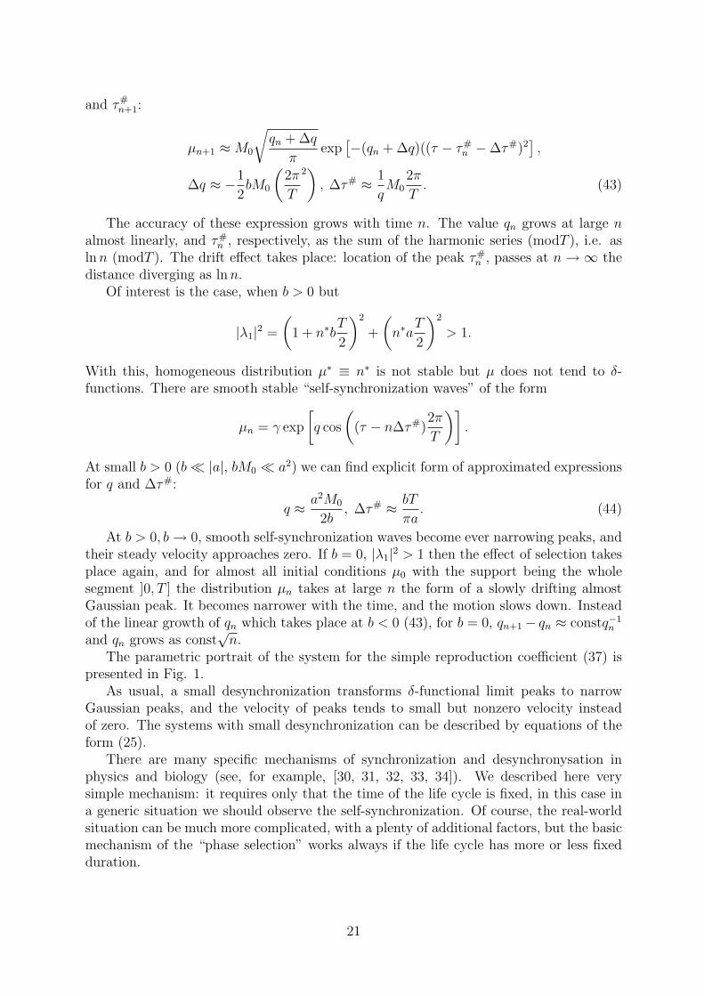
At b > 0, b → 0, smooth self-synchronization waves become ever narrowing peaks, andtheir steady velocity approaches zero. If b = 0, |λ1|2 > 1 then the effect of selection takesplace again, and for almost all initial conditions µ0 with the support being the wholesegment ]0, T ] the distribution µn takes at large n the form of a slowly drifting almostGaussian peak. It becomes narrower with the time, and the motion slows down. Insteadof the linear growth of qn which takes place at b < 0 (43), for b = 0, qn+1− qn ≈ constq−1

n

and qn grows as const√

n.The parametric portrait of the system for the simple reproduction coefficient (37) is

presented in Fig. 1.As usual, a small desynchronization transforms δ-functional limit peaks to narrow

Gaussian peaks, and the velocity of peaks tends to small but nonzero velocity insteadof zero. The systems with small desynchronization can be described by equations of theform (25).

There are many specific mechanisms of synchronization and desynchronysation inphysics and biology (see, for example, [30, 31, 32, 33, 34]). We described here verysimple mechanism: it requires only that the time of the life cycle is fixed, in this case ina generic situation we should observe the self-synchronization. Of course, the real-worldsituation can be much more complicated, with a plenty of additional factors, but the basicmechanism of the “phase selection” works always if the life cycle has more or less fixedduration.

21

n*bT/2

n*aT/2

Stableuniformdistribution

Stable waveswith non-zerovelocity

v≈≈≈≈b/( ππππa)

Waves with velocity

Vn ÷÷÷÷1/n →→→→0

v

Figure 1: The simplest model of cell division self-synchronization: The parametric por-trait.

References

[1] Darwin, Ch., On the origin of species by means of natural selection, or preservationof favoured races in the struggle for life: A Facsimile of the First Edition, Harvard,1964. http://www.literature.org/authors/darwin-charles/the-origin-of-species/

[2] Haldane, J.B.S., The Causes of Evolution, Princeton Science Library, Princeton Uni-versity Press, 1990.

[3] Mayr, E., Animal Species and Evolution. Cambridge, MA: Harvard University Press,1963.

[4] Ewens, W.J., Mathematical Population Genetics. Springer-Verlag, Berlin, 1979.

[5] Rozonoer, L.I., Sedyh, E.I., On the mechanisms of of evolution of self-reproductionsystems, 1, Automation and Remote Control, 40, 2 (1979), 243–251; 2, ibid., 40, 3(1979), 419–429; 3, ibid, 40, 5 (1979), 741-749.

[6] Gorban, A.N., Dynamical systems with inheritance, in: Some problems of commu-nity dynamics, R.G. Khlebopros (ed.), Institute of Physics RAS, Siberian Branch,Krasnoyarsk, 1980 [in Russian].

[7] Gorban, A. N., Equilibrium encircling. Equations of chemical kinetics and their ther-modynamic analysis, Nauka, Novosibirsk, 1984 [in Russian].

[8] Semevsky, F.N., Semenov S.M., Mathematical modeling of ecological processes,Gidrometeoizdat, Leningrad, 1982 [in Russian].

[9] Gorban, A.N., Khlebopros, R.G., Demon of Darwin: Idea of optimality and naturalselection, Nauka (FizMatGiz), Moscow, 1988 [in Russian].

22

[10] Zakharov, V.E., L’vov, V.S., Starobinets, S.S., Turbulence of spin-waves beyondthreshold of their parametric-excitation, Uspekhi Fizicheskikh Nauk 114, 4 (1974),609–654; English translation Sov. Phys. - Usp. 17, 6 (1975), 896–919.

[11] Zakharov, V.E., L’vov, V.S., Falkovich, G.E., Kolmogorov spectra of turbulence, vol.1 Wave Turbulence. Springer, Berlin, 1992.

[12] L’vov, V.S., Wave turbulence under parametric excitation applications to magnets,Springer, Berlin, Heidelberg, 1994.

[13] Ezersky A.B., Rabinovich M.I., Nonlinear-wave competition and anisotropic spectraof spatiotemporal chaos of Faraday ripples, Europhysics Letters 13, 3 (1990), 243–249.

[14] Krawiecki, A, Sukiennicki, A., Marginal synchronization of spin-wave amplitudes ina model for chaos in parallel pumping, Physica Status Solidi B–Basic Research 236,2 (2003), 511–514.

[15] Vorobev, V.M., Selection of normal variables for unstable conservative media, Zhur-nal Tekhnicheskoi Fiziki, 62, 8 (1992), 172–175.

[16] Seminozhenko, V.P., Kinetics of interacting quasiparticles in strong external fields.Phys. Reports, 91, 3 (1982), 103–182.

[17] Haken, H., Synergetics, an introduction. Nonequilibrium phase transitions and self–organization in physics, chemistry and biology, Springer, Berlin, Heidelberg, NewYork, 1978.

[18] Bourbaki, N., Elements of mathematics - Integration I, Springer, Berlin, Heidelberg,New York, 2003.

[19] Smale, S., Structurally stable systems are not dense, Amer. J. Math., 88 (1966),491–496.

[20] Birkhoff, G.D., Dynamical systems, AMS Colloquium Publications, Providence,1927. Online: http://www.ams.org/online bks/coll9/

[21] Hasselblatt, B., Katok, A. (Eds.), Handbook of Dynamical Systems, Vol. 1A, Else-vier, 2002.

[22] Katok, A., Hasselblat, B., Introduction to the Modern Theory of Dynamical Systems,Encyclopedia of Math. and its Applications, Vol. 54, Cambridge University Press,1995.

[23] Levin, L.A., Randomness conservation inequalities; Information and independencein mathematical theories, Information and Control, 61, 1 (1984), 15–37.

[24] Gause, G.F., The struggle for existence, Williams and Wilkins, Baltimore, 1934.Online: http://www.ggause.com/Contgau.htm.

[25] Volterra, V., Lecons sur la theorie mathematique de la lutte pour la vie, Gauthier-Villars, Paris, 1931.

23

[26] Gromov, M., A dynamical model for synchronisation and for inheritance in micro-evolution: a survey of papers of A.Gorban, The talk given in the IHES seminar,“Initiation to functional genomics: biological, mathematical and algorithmical as-pects”, Institut Henri Poincare, November 16, 2000.

[27] Kuzenkov, O.A., Weak solutions of the Cauchy problem in the set of Radon proba-bility measures, Differential Equations, 36, 11 (2000), 1676–1684.

[28] Kuzenkov, O.A., A dynamical system on the set of Radon probability measures,Differential Equations, 31, 4 (1995), 549–554.

[29] Diekmann, O. A beginner’s guide to adaptive dynamics, in: Mathematical modellingof population dynamics, Banach Center Publications, V. 63, Institute of MathematicsPolish Academy of Sciences, Warszawa, 2004, 47–86.

[30] Blekhman, I.I., Synchronization in science and technology. ASME Press, N.Y., 1988.

[31] Pikovsky, A., Rosenblum, M., Kurths, J., Synchronization: A Universal Concept inNonlinear Science, Cambridge University Press, 2002.

[32] Josic, K., Synchronization of chaotic systems and invariant manifolds, Nonlinearity13 (2000) 1321-1336.

[33] Mosekilde, E., Maistrenko, Yu., Postnov, D., Chaotic synchronization: Applicationsto living systems, World Scientific, Singapore, 2002.

[34] Cooper, S., Minimally disturbed, multi-cycle, and reproducible synchrony using aeukaryotic “baby machine”, Bioessays 24 (2002), 499–501.

24