A KAM Theorem for Hamiltonian Partial Differential Equations with Unbounded Perturbations * Jianjun Liu, Xiaoping Yuan School of Mathematical Sciences and Key Lab of Math. for Nonlinear Science, Fudan University, Shanghai 200433, P R China September 30, 2010 Abstract: We establish an abstract infinite dimensional KAM theorem dealing with unbounded perturbation vector-field, which could be applied to a large class of Hamiltonian PDEs containing the derivative ∂ x in the perturbation. Especially, in this range of application lie a class of derivative nonlinear Schr¨ odinger equations with Dirichlet boundary conditions and perturbed Benjamin-Ono equation with periodic boundary conditions, so KAM tori and thus quasi-periodic solutions are ob- tained for them. 1 Introduction and Main Results Consider a Hamiltonian partial differential equation (HPDE) ˙ w = Aw + F (w), where Aw is linear Hamiltonian vector-field with d := ord A > 0 and F (w) is nonlinear Hamiltonian vector-field with ˜ d := ord F and is analytic in the neighborhood of the origin w = 0. When ˜ d = ord F ≤ 0, the vector-field F is called bounded perturbation. For example, in this case lie a class of nonlinear Schr ¨ odinger equations (with ˜ d = 0) iu t + u xx + V (x)u + |u| 2 u = 0 and a class of nonlinear wave equations (with ˜ d = -1) u tt - u xx + V (x)u + u 3 = 0. For the existence of KAM tori of the PDEs with bounded perturbations has been deeply and widely investigated by many authors. In this field of study there are too many references to list here. We give just two survey papers by Kuksin [8] and Bourgain [4]. When ˜ d = ord F > 0, the vector-field F is called unbounded perturbation. According to a well- known example, due to Lax [11] and Klainerman [5] (See also [7]), it is reasonable to assume ˜ d ≤ d - 1 in order to guarantee the existence of KAM tori for the PDE. The quantity d - ˜ d measures the strength of nonlinearity of the PDE. The smaller the d - ˜ d is, the stronger the nonlinearity is. When d - ˜ d = 1, the nonlinearity of the PDE is the strongest. * Supported by NNSFC and 973 Program (No. 2010CB327900) and the Research Foundation for Doctor Programme. 1
Transcript
A KAM Theorem for Hamiltonian Partial DifferentialEquations with Unbounded Perturbations ∗
Jianjun Liu, Xiaoping YuanSchool of Mathematical Sciences and Key Lab of Math. for Nonlinear Science,
Fudan University, Shanghai 200433, P R China
September 30, 2010
Abstract: We establish an abstract infinite dimensional KAM theorem dealing with unboundedperturbation vector-field, which could be applied to a large class of Hamiltonian PDEs containingthe derivative ∂x in the perturbation. Especially, in this range of application lie a class of derivativenonlinear Schrodinger equations with Dirichlet boundary conditions and perturbed Benjamin-Onoequation with periodic boundary conditions, so KAM tori and thus quasi-periodic solutions are ob-tained for them.
1 Introduction and Main ResultsConsider a Hamiltonian partial differential equation (HPDE)
w = Aw+F(w),
where Aw is linear Hamiltonian vector-field with d := ord A > 0 and F(w) is nonlinear Hamiltonianvector-field with d := ord F and is analytic in the neighborhood of the origin w = 0.
When d = ord F ≤ 0, the vector-field F is called bounded perturbation. For example, in this caselie a class of nonlinear Schrodinger equations (with d = 0)
iut +uxx +V (x)u+ |u|2u = 0
and a class of nonlinear wave equations (with d =−1)
utt −uxx +V (x)u+u3 = 0.
For the existence of KAM tori of the PDEs with bounded perturbations has been deeply and widelyinvestigated by many authors. In this field of study there are too many references to list here. Wegive just two survey papers by Kuksin [8] and Bourgain [4].
When d = ord F > 0, the vector-field F is called unbounded perturbation. According to a well-known example, due to Lax [11] and Klainerman [5] (See also [7]), it is reasonable to assume
d ≤ d−1
in order to guarantee the existence of KAM tori for the PDE. The quantity d − d measures thestrength of nonlinearity of the PDE. The smaller the d− d is, the stronger the nonlinearity is. Whend− d = 1, the nonlinearity of the PDE is the strongest.
∗Supported by NNSFC and 973 Program (No. 2010CB327900) and the Research Foundation for Doctor Programme.
1
For the PDE with unbounded Hamiltonian perturbation, the only previous KAM theorem is dueto Kuksin [7] where it is assumed that d − d > 1. Kuksin’s theorem is in [7] used to prove thepersistence of the finite-gap solutions of KdV equation, as well as its hierarchy, subject to periodicboundary conditions. See also Kappeler-Poschel [10]. Another KAM theorem with unboundedlinear Hamiltonian perturbation is due to Bambusi-Graffi [2] where the spectrum property is inves-tigated for the time dependent linear Schrodinger equation
iy(t) = (A+ εF(t))y(t)
with d− d > 1 also.The assumption d− d > 1 excludes a large class of interesting partial differential equations such
as a class of derivative nonlinear Schrodinger (DNLS) equations
iut +uxx−Mσ u+ i f (u, u)ux = 0
subject to Dirichlet boundary conditions, and perturbed Benjamin-Ono (BO) equation
ut +H uxx−uux +perturbation = 0
subject to periodic boundary conditions, where H is the Hilbert transform. In both cases, d− d =1. In the present paper, we will construct a KAM theorem including d− d > 1 and limiting cased− d = 1 and show the existence of KAM tori for DNLS and perturbed BO equations.
If the Hamiltonian operator A has continuous spectra, there is usually no KAM tori for the HPDE.Therefore, we should assume that the Hamiltonian operator A is of pure point spectra before statingour theorems. Taking the eigenfunctions of A as a basis and changing partial coordinates into action-angle variables, from the HPDE one can usually obtain a small perturbation H = N +P of an infinitedimensional Hamiltonian in the parameter dependent normal form
N = ∑1≤ j≤n
ω j(ξ )y j +12 ∑
j≥1Ω j(ξ )(u2
j + v2j) (1.1)
on a phase spacePa,p = Tn×Rn× `a,p× `a,p 3 (x,y,u,v)
with symplectic structure ∑1≤ j≤n dy j∧dx j +∑ j≥1 du j∧dv j, where `a,p is the Hilbert space of all realsequences w = (w1,w2, · · ·) with
‖w‖2a,p = ∑
j≥1e2a j j2p|w j|2 < ∞,
where a ≥ 0 and p ≥ 0. The tangential frequencies ω = (ω1, · · · ,ωn) and normal frequencies Ω =(Ω1,Ω2, · · ·) are real vectors depending on parameters ξ ∈ Π ⊂ Rn, Π a closed bounded set ofpositive Lebesgue measure, and roughly
Ω j(ξ ) = jd + · · · .The perturbation term P is real analytic in the space coordinates and Lipschitz in the parameters,
and for each ξ ∈ Π its Hamiltonian vector field XP = (Py,−Px,−Pv,Pu)T defines near T0 := Tn×y = 0×u = 0×v = 0 a real analytic map
XP : Pa,p →Pa,q,
wherep−q = d.
2
In the whole of this paper the parameter a is fixed. Moreover, throughout this paper, for convenience,we will adopt lots of notations and definitions from [10].
We denote by Pa,pC the complexification of Pa,p. For s,r > 0, We introduce the complex T0-
where |·| denotes the sup-norm for complex vectors. Furthermore, for a map W : D(s,r)×Π→Pa,qC ,
for example, the Hamiltonian vector field XP, we define the norms
‖W‖r,a,q,D(s,r)×Π = supD(s,r)×Π
‖W‖r,a,q,
‖W‖lipr,a,q,D(s,r)×Π = sup
ξ ,ζ∈Π,ξ 6=ζsup
D(s,r)
‖∆ξ ζW‖r,a,q
|ξ −ζ | ,
where ∆ξ ζW = W (·;ξ )−W (·;ζ ). In a completely analogous manner, the Lipschitz semi-norm ofthe frequencies ω and Ω are defined as
|ω|lipΠ = supξ ,ζ∈Π,ξ 6=ζ
|∆ξ ζ ω||ξ −ζ | , |Ω|lip−δ ,Π = sup
ξ ,ζ∈Π,ξ 6=ζsupj≥1
j−δ |∆ξ ζ Ω j||ξ −ζ | (1.3)
for any real number δ .
Theorem 1.1. Suppose the normal form N described above satisfies the following assumptions:
(A) The map ξ 7→ ω(ξ ) between Π and its image is a homeomorphism which is Lipschitz contin-uous in both directions, i.e. there exist positive constants M1 and L such that |ω|lipΠ ≤M1 and|ω−1|lipω(Π) ≤ L;
(B) There exists d > 1 such that|Ωi−Ω j| ≥ m|id − jd | (1.4)
for all i 6= j ≥ 0 uniformly on Π with some constant m > 0. Here Ω0 = 0;
(C) There exists δ ≤ d− 1 such that the functions ξ 7→ Ω j(ξ )jδ
are uniformly Lipschitz on Π for
j ≥ 1, i.e. there exist a positive constant M2 such that |Ω|lip−δ ,Π ≤M2;
(D) We additionally assume4ELM2 ≤ m, (1.5)
where E = |ω|Π := supξ∈Π |ω(ξ )|.Set M = M1 + M2. Then for every β > 0, there exists a positive constant γ , depending only onn,d,δ ,m, the frequencies ω and Ω, s > 0 and β , such that for every perturbation term P describedabove with
d = p−q≤ d−1 (1.6)
andε := ‖XP‖r,a,q,D(s,r)×Π +
αM‖XP‖lip
r,a,q,D(s,r)×Π ≤ (αγ)1+β (1.7)
for some r > 0 and 0 < α < 1, there exist
3
(1) a Cantor set Πα ⊂Π with|Π\Πα | ≤ c1α, (1.8)
where | · | denotes Lebesgue measure and c1 > 0 is a constant depends on n, ω and Ω;
(2) a Lipschitz family of smooth torus embeddings Φ : Tn ×Πα → Pa,p satisfying: for everynon-negative integer multi-index k = (k1, . . . ,kn),
‖∂ kx (Φ−Φ0)‖r,a,p,Tn×Πα +
αM‖∂ k
x (Φ−Φ0)‖lipr,a,p,Tn×Πα
≤ c2ε1
1+β /α, (1.9)
where ∂ kx := ∂ |k|
∂xk11 ···∂xkn
nwith |k| := |k1|+ · · ·+ |kn|,
Φ0 : Tn×Π→T0, (x,ξ ) 7→ (x,0,0,0)
is the trivial embedding for each ξ , and c2 is a positive constant which depends on k and thesame parameters as γ;
(3) a Lipschitz map φ : Πα → Rn with
|φ −ω|Πα +αM|φ −ω|lipΠα
≤ c3ε, (1.10)
where c3 is a positive constant which depends on the same parameters as γ ,
such that for each ξ ∈ Πα the map Φ restricted to Tn×ξ is a smooth embedding of a rotationaltorus with frequencies φ(ξ ) for the perturbed Hamiltonian H at ξ . In other words,
t 7→Φ(θ + tφ(ξ ),ξ ), t ∈ Ris a smooth quasi-periodic solution for the Hamiltonian H evaluated at ξ for every θ ∈ Tn andξ ∈Πα .
This theorem can be applied to the class of derivative nonlinear Schrodinger equations mentionedabove. However, the assumption (1.5) excludes the perturbed Benjamin-Ono equation mentionedabove. Thus, in the following, we give a modified version of the above theorem:
Theorem 1.2. The above theorem also holds true with, respectively, replacing the assumption (D)and conclusion (1) by the assumption (D*) and conclusion (1*) below:
(D*) For every k ∈ Zn and l ∈ Z∞ with 1≤ |l| ≤ 2 (here |l|= ∑ j≥1 |l j|), the resonance set
ξ ∈Π : 〈k,ω(ξ )〉+ 〈l,Ω(ξ )〉= 0has Lebesgue measure zero; Moreover, if δ = d− 1, we additively assume that there existδ0 < d−1, a partition Ω = Ω1 +Ω2, positive constant M3 and M4 with
8ELM4 ≤ m, (1.11)
such that |Ω1|lip−δ0,Π ≤M3, |Ω2|lip−δ ,Π ≤M4;
(1*) a Cantor set Πα ⊂Π with |Π\Πα | → 0 as α → 0, where | · | denotes Lebesgue measure.
This paper is organized as follows: In section 2 we give an outline of the proof of the abovetheorems, and some new difficult and ideas compared with [7] [10] are exhibited. In sections 3-6the above theorems are proved in detail. The proof of Theorem 1.2 is the same as that of Theorem1.1 except the measure estimate. Thus, sections 3-5 and subsection 6.1 are devoted to the proof ofTheorem 1.1, while the measure estimate for Theorem 1.2 is given in subsection 6.2. In sections7-8 Theorem 1.1 and Theorem 1.2 are applied to derivative nonlinear Schrodinger equations andperturbed Benjamin-Ono equation, respectively. Finally, a technical lemma is listed in section 9.
4
2 Outline of The Proof and more RemarksThe above theorems generalize Kukisn’s theorem from d < d− 1 to d ≤ d− 1 such that the rangeof application is extended to a class of derivative nonlinear Schrodinger equations and perturbedBenjamin-Ono equation. Here we would like to compare the proof of our theorems with that ofKuksin’s theorem. By and large, as any KAM theorem, in both cases Newton iteration is used toovercome the notorious small divisor difficult. Therefore, our proof is mainly based on Kuksin’sapproach in [7]. (Also see [10]). There is, however, some essential differences between the proofof our theorems and that of Kuksin’s theorem. In order to see clearly the differences, let us give thebasic procedure of the proof of KAM theorem from [7] and [10], which consists of the followingsteps.
2.1. Derivation of the homological equations. For convenience, introduce complex variablesz = (u− iv)/
√2 and z = (u+ iv)/
√2. Assume we are now in the ν-th KAM iterative step. Write the
integrable part Nν of the Hamiltonian Hν
Nν = 〈ω,y〉+∞
∑j=1
Ω jz j z j
and develop the perturbation Pν into Taylor series in (y,z, z):
Pν = εν Rν +O(|y|2 + |y|||z||a,p + ||z||3a,p),
where εν goes to zero very fast, for example, taking εν ≈ ε(5/4)ν, and
νRν ,Fν+ · · · .Our task is now to search for Fν satisfying Nν ,Fν+ Rν = 0 which is a set of the first order
partial differential equations:
ω ·∂xFx(x) = Rx(x), ω ·∂xFy(x) = Ry(x),
· · ·ω ·∂xFzz(x)+ iΛFzz(x)− iFzz(x)Λ = Rzz(x),
5
where Λ = diag (Ω j : j = 1,2, ...). Let us consider the last equation which is the most difficulty one.By Fi j(x) and Ri j(x), denote the matrix elements of the operators Fzz and Rzz, respectively. Then thelast equation becomes
where Fi j(k) and Ri j(k) are the k-th Fourier coefficients of Fi j(x) and Ri j(x), respectively. One canassume R j j(0) = 0, otherwise R j j(0) is put into Ω j as a modification of the normal form Nν . Thus,(2.3) can be solved by
Fi j(k) =Ri j(k)
〈k,ω〉+Ωi−Ω j
under the non-resonant conditions
〈k,ω〉+Ωi−Ω j 6= 0 unless k = 0, i = j.
This is actually the KAM iterative procedure for bounded perturbation P. However, the thing is notso simple when the perturbation P is unbounded, i.e., d = p−q > 0. When
XP : Pa,p →Pa,q, d = p−q > 0,
one has, very roughly,|Ri j(k)|≈ |i|d + | j|d → ∞, as |i|+ | j| → ∞.
This leads usually to Fi j(k)→ ∞. In other words, the solution Fν or the transformation Φν = X1εν Fν
would be unbounded. One should note that the coordinate transformations Φν = X1εν Fν must be
bounded even if the the perturbation P is unbounded in order that the domains of the KAM iterationare always in the same phase space Pa,p and that the KAM iterative procedure can work. In orderto guarantee the bounded-ness of Fν , it is required in [7] and [10] that
|Ωi−Ω j|≈ |i|d−1 + | j|d−1, i 6= j
or rather roughly,|〈k,ω〉+Ωi−Ω j|≈ |i|d−1 + | j|d−1.
Together with d ≤ d−1, one has that for i 6= j,
|Fi j(k)|≈ |i|d + | j|d|i|d−1 + | j|d−1 = O(1).
It is clear that this estimate fails when i = j. To avoid this plight, Kuksin[7] smartly put the wholeR j j(x) rather than R j j(0) into Ω j as a modification of the normal form Nν so that it is not necessaryto solve the equation for Fj j(x). In doing so, the term Nν becomes into the generalized normal form(i.e. normal frequencies depend on the angle variable x)
Nν := Nν +∞
∑j=1
R j j(x)z j z j = 〈ω,y〉+∞
∑j=1
(Ω j +R j j(x))z j z j,
the homological equation (2.1) is modified into
Nν ,Fν+Rν = 0, (2.4)
6
and the remaining term Rν+1 is changed into
Rν+1 =12
ε2νNν ,Fν,Fν+ ε2
νRν ,Fν+ · · · . (2.5)
Accordingly, the homological equation (2.3) becomes into
−iω ·∂xFi j(x)+(Ωi−Ω j +Rii(x)−R j j(x))Fi j(x) =−iRi j(x), i 6= j. (2.6)
Let u = Fi j(x), λ = Ωi−Ω j, µ(x) = Rii(x)−R j j(x) and r(x) =−iRi j(x). Then this equation can beabbreviated as an abstract equation
−iω ·∂xu+(λ + µ(x))u = r(x). (2.7)
Since Rii and R j j are large, µ(x) is usually large. And the coefficient µ(x) involves the angle variable.The equation of this type is called “small-denominators equations with large variable coefficients”by Kuksin [6]. Remark that, for simplicity, the modification of ω is omitted here.
2.2. Solving the homological equations. In order to make KAM iterative procedure work, theexistence domain of the solution u should be the strip-type neighborhood of Tn with some widths > 0: D(s) := x ∈ Cn/2πZn : |Im x| ≤ s. Assume
µ(x)≈Cγ,
where C is some small constant and where γ should be usually a large magnitude. Since (2.7) isscalar, it can be solved directly and estimated by
supx∈D(s−σ)
|u(x)|. e2Cγ ||r||s, 0≤ σ < s, (2.8)
where ‖r‖s := supx∈D(s) |r(x)|. This estimate is, however, not good enough to support the KAMiteration procedure, since the solution u becomes too large as µ is large. In fact, in the ν-th KAMiteration step, γ ≈ 2ν . Thus, u ≈ exp(2ν) goes to infinity very rapidly, which makes the coordinatetransformations essentially unbounded. When d < d−1, Kuksin’s lemma [6] can solve this problem.Following Kuksin [6], we assume there are constant C > 0 and 0 < θ < 1 such that
|λ |θ ≥C‖µ‖s, (2.9)
Kuksin’s Lemma states that under suitable non-resonant conditions on ω , the solution u satisfies theestimate:
‖u‖s−σ ≤C1 exp(C2C1
1−θ3 )||r||s, (2.10)
where C1 and C2 are positive constants depending on only n and σ , and C3 > 0 is a constant depend-ing on the non-resonant conditions. When this estimate is applied to (2.6), one needs to take
λ = Ωi−Ω j ≈ id − jd ≈ id−1 + jd−1, γ ≈ id + jd , i, j = 1,2,3, . . . .
From this, we see that there is indeed a constant 0 < θ < 1 such that (2.9) holds true if d < d− 1.Therefore, the solution u of the homological equation (2.7) has a uniform bound independent of thesize of µ . This makes the coordinate transformation bounded. We see also that d = d− 1 leads toθ = 1 in (2.9). In this case, the estimate (2.10) is invalid. (The right hand side of (2.10) is equal to∞.) Now it is clear that we need some new estimate for the solution u covering not only the cased < d−1 but also the limit case d = d−1. The new estimate has been obtained in our recent paper[12]:
‖u‖s−σ ≤C4eCγs‖r‖s, (2.11)
7
where C4 is a constant depending the non-resonant conditions on ω and where C is a positive constantsmall enough. Since the parameter γ (which measures the magnitude of the perturbation µ(x)) goesinto the exponential in the right hand side of (2.11), in this sense, the upper bound of this newestimate looks weaker than that of the original Kuksin’s lemma. However, compared with (2.8),there is some essential improvement in (2.11): there is an s in the exponential in (2.11). This numbers will be used crucially in the following manner: In the ν-th KAM iteration, we let s = 2−ν . Onewill find that there is no the small divisor problem in the homological equation (2.7) when γ > somelarge constant K ≈ 2ν(5/4)ν | lnε|. In this case, the homological equation (2.7) can be solved by theimplicit function theorem. So the non-trivial case is when γ ≤ K. At this time, we find that
eCγs . ε−Cν
with εν := ε(5/4)νand the constant C ¿ 1. Thus, by the new estimate (2.11) and noting ||r||s ≤ εν ,
we have‖u‖s−σ . ε−C
ν ||r||s ≤ ε−Cν εν . εν . (2.12)
In the usual KAM iteration, one would have obtained ||u||s−σ ≤ 2ν εν . εν . Although here ε−Cν εν À
2ν εν , inequality (2.12) can guarantee the KAM procedure to be iterated. Therefore, although thenew estimate (2.11) is weaker than that of the original Kuksin’s Lemma, it can covers both d < d−1and the limit case d = d− 1, and it is sufficient for the proof of the KAM theorems of the presentpaper.
2.3. Estimate of the remaining terms Rν+1, etc. Recall Rν = O(1). By (2.11), Fν = O(ε−Cν ) with
0 < C ¿ 1. Thus,Fν ,Rν= O(ε−C
ν ).
By (2.4),Nν ,Fν=−Rν = O(1).
Thus,Nν ,Fν,Fν= O(1),O(ε−C
ν )= O(ε−Cν ).
Consequently, by (2.5), very roughly,
Rν+1 =12
ε2νN,Fν,Fν+ ε2
νRν ,Fν+ · · ·= O(ε2−Cν ) = O(εν+1) := εν+1Rν+1,
where Rν+1 = O(1). Therefore, we can rewrite Hν+1 as
where N∞ = limν→∞ Nν = 〈ω∞,y〉+∑ j≥1 Ω∞, j(x)z j z j. The system corresponding to H∞ is
x = ∂H∞∂y = ω∞ +O(|y|+ ||z||a,p)
y =− ∂H∞∂x = O(|y|2 + |y|||z||a,p + ||z||2a,p)
z j =−i ∂H∞∂ z j
=−iΩ∞, jz j +O(|y|+ ||z||2a,p), j ≥ 1.
It is clearly seen that
T∞ := (x,y,z, z) ∈Pa,p : x = ω∞t,y = 0,z = z = 0, t ∈ R
8
forms an invariant torus of the hamiltonian vector field XH∞ . Going back to the original vector fieldXH , then (limν→∞ Φ1 · · · Φν)T∞ is an invariant torus of the Hamiltonian system defined by H.
2.5. Estimate of the measure of the parameters. When d = d−1, another new difficult also arisesin search for F . It is under suitable non-resonant conditions that either (2.11) or (2.10) can hold true.In other words, one has to remove some resonant sets consisting of “bad” parameters ξ , equivalently,to remove the “bad” parameters ω when ω = ω(ξ ) depends on ξ in some non-degenerate way. Forexample, we need to eliminate the resonant set
ξ ∈Π : 〈k,ω(ξ )〉+Ωi(ξ )−Ω j(ξ ) is smallwhere i 6= j ∈ N and k ∈ Zn. Clearly we hope that the Lebesgue measure of the set is small. To thatend we need to verify that 〈k,ω(ξ )〉+Ωi(ξ )−Ω j(ξ ) is twisted with respect to ξ ∈Π, equivalently,twisted with respect to ω ∈ ω(Π), that is, we need to show
(?) := |〈k,ω〉+Ωi(ξ (ω))−Ω j(ξ (ω))|lipω(Π) > 0,
where ω(ξ (ω)) = ω .Recall |Ωi−Ω j| ≥ m|id − jd |. Thus, 〈k,ω〉+Ωi−Ω j is not small if |k| ≤ C0|id − jd | with some
constant C0 depending on m and |ω|Π. Now we assume |k| ≥ C0|id − jd |. At the ν-th KAM step,because of the modification of frequencies from unbounded perturbation, we have
|Ω j|lipω(Π) = O( jδ )+O( jd).
By a small trick (See §3.2 below.), we can let δ = d . Therefore, there exists a constant C1 such that
(?) ≥ |k|−C1(id + jd) (2.14)
≥ 12
C0(id−1 + jd−1)−C1(id + jd) (2.15)
≥(1
4C0(id−1−d + jd−1−d)−C1
)(id + jd), (2.16)
which is similar to (10.50) in [7] (See also page 174 in [10]). When d < d−1, it follows from (2.16)that (?) > 0 if
max(i, j) >(4C1
C0
) 1d−1−d := K . (2.17)
Therefore, if d < d−1 it remains to verify the twist condition (?) > 0 just for only finite number ofcases
(k, i, j) : C0|id − jd | ≤ |k| ≤ C1(id + jd) and i, j ≤K . (2.18)
Note that the constant K is independent of i, j and k, so is the number of the cases. For these cases,the measure estimate of the resonant sets can be dealt with by some initial assumptions (For example,see Proposition 22.2 in [10]). When d = d−1, K = +∞. However, it follows directly from (2.15)that (?) > ( 1
2C0− C1)(id−1 + jd−1) > 0 if C0 > 2C1. This completes the measure estimate of theresonant sets for Theorem 1.1. One can verify that the condition C0 > 2C1 is indeed satisfied byDNLS equations.
However, the inequality C0 > 2C1 is not satisfied by BO equation. The procedure of the measureestimate of the resonant set is modified as follows:
Assume that Ω can be split into two part: Ω j = Ω1j + Ω2
j such that |Ω1j |lipω(Π) ≤ C2 jδ0 with δ0 <
d−1, and |Ω2j |lipω(Π) ≤ C3 jd−1 with C3 suitably small. Thus,
(?)≥(|k|−C2(iδ0 + jδ0)−C3(id−1 + jd−1)
)
≥ (12
C0−C3)(id−1 + jd−1)−C2(iδ0 + jδ0).
9
It follows from δ0 < d− 1 that there is a constant ˜K = ˜K (d,δ0,C0,C2,C3) > 0 such that (?) > 0if maxi, j > ˜K and 1
2C0 > C3. The latter inequality is satisfied by BO equation with d = 2 andδ0 = 0. We also mention that the partition of Ω into Ω1 +Ω2 is rather natural. In fact, Ω1 is usuallyregarded as the initial frequency vector, while Ω2 corresponds to the modification in KAM iterationsteps.
Remarks. 1. In [12] we mentioned Theorem 1.1 above and its application to DNLS equationwithout proof. In this paper we give the proof and add Theorem 1.2 and a new application toBenjamin-Ono equation.
2. The proofs of both (2.10) and (2.11) depends heavily on the fact that the homological equation(2.7) is 1-dimensional so that the solution can be expressed explicitly. This dimensional restrictionrequires that the normal frequency Ω j’s must be simple, i.e., Ω]
j = 1. Therefore, the range of ap-plication of Theorems 1.1 and 1.2 and Kuksin’s KAM theorem ([7]) lies in those PDEs with simplefrequencies such as DNLS equation subject to Dirichlet boundary conditions, KdV and BO equa-tions with periodic boundary conditions. For a class of DNLS equation
iut +uxx−Mσ u+ i(|u|2u)x = 0
subject to periodic boundary conditions, the multiplicity Ω]j = 2. And for Kadomtsev-Petviashvili
its frequency multiplicity Ω]j →∞ as | j| →∞. There is nothing to know about the existence of KAM
tori for these two classes of PDEs with perturbations. In particular, the existence of KAM tori forKP equation is a well-known open problem by Kuksin. See [8],[4].
3 The Homological Equations
3.1 Derivation of Homological EquationsThe proof of Theorem 1.1 employs the rapidly converging iteration scheme of Newton type to dealwith small divisor problems introduced by Kolmogorov, involving infinite sequence of coordinatetransformations. At the ν-th step of the scheme, a Hamiltonian
Hν = Nν +Pν
is considered, as a small perturbation of some normal form Nν . A transformation Φν is set up so that
Hν Φν = Nν+1 +Pν+1
with another normal form Nν+1 and a much smaller perturbation Pν+1. We drop the index ν of Hν ,Nν , Pν , Φν and shorten the index ν +1 as +.
Using convenient complex notation z = (u− iv)/√
2 and z = (u+ iv)/√
2, the generalized normalform reads
N = 〈ω(ξ ),y〉+ ∑j≥1
Ω j(x;ξ )z j z j. (3.1)
Let R be 2-order Taylor polynomial truncation of P, that is,
where 〈·, ·〉 is formal product for two column vectors and Rx, Ry, Rz, Rz, Rzz, Rzz, Rzz depend on xand ξ . For a function u on Tn, let
[u] =1
(2π)n
∫
Tnu(x)dx.
10
By [R] denote the part of R in generalized normal form as follows
[R] = [Rx]+ 〈[Ry],y〉+ 〈diag(Rzz)z, z〉,
where diag(Rzz) is the diagonal of Rzz. Note that [Rx] and [Ry] are independent of x. In the following,the term [Rx] will be omitted since it does not affect the dynamics.
The coordinate transformation Φ is obtained as the time-1-map X tF |t=1 of a Hamiltonian vector
field XF , where F is of the same form as R:
F = Fx + 〈Fy,y〉+ 〈Fz,z〉+ 〈F z, z〉+ 〈Fzzz,z〉+ 〈F zzz, z〉+ 〈Fzzz, z〉, (3.3)
Moreover, for an analytic function u on D(s), we define
|u|s,τ := ∑k∈Zn
|uk||k|τ e|k|s,
where uk := (2π)−n ∫Tn u(x)e−ik·xdx is the k-Fourier coefficient of u.
Consider the conditions δ ≤ d−1 and d = p−q≤ d−1. If δ > d, decreasing q such that δ = d,then for the new q, the inequality (1.7) still holds true; if δ < d, increasing δ such that δ = d, thenfor the new δ , the assumption (C) still holds true, and if d = d−1, the assumption (D*) is satisfiedwith Ω2 = 0. Thus, without loss of generality we assume δ = d ≤ d−1 in the following.
Equations (3.13)-(3.19) will be solved under the following conditions: uniformly on Π,
with constants τ ≥ n, d > 1, 0 < γ0 ≤ 1/8, m > 0, and a parameter 0 < α ≤m. We mention that d isthe same as in Theorem 1.1 and α , m will be the iteration parameters αν , mν in the ν-th KAM step.
Equations (3.13) (3.14) can be easily solved by a standard approach in classical, finite dimen-sional KAM theory, so we only give the related results at the end of this subsection. Equations(3.15)-(3.18) are easier than (3.19) and can be solved in the same way as (3.19) done, so we onlygive the details of solving (3.19) in the following.
For any positive number K, we introduce a truncation operator ΓK as follows:
(ΓK f )(x) := ∑|k|≤K
fkeik·x, ∀ f : Tn → C,
where fk is the k-Fourier coefficient of f .Set C0 = 2|ω|Π/m and K being a positive number which will be the iteration parameter Kν in
the ν-th KAM step.
(1) For (i, j) with 0 < |id − jd |< C0K, we solve exactly (3.19):
∂ω Fzzi j + i(Ωi−Ω j)Fzz
i j = Rzzi j ; (3.23)
(2) for (i, j) with |id − jd | ≥C0K, we solve the truncated equation of (3.19):
∂ω Fzzi j + iΓK
((Ωi−Ω j)Fzz
i j
)= ΓKRzz
i j , ΓKFzzi j = Fzz
i j . (3.24)
Comparing (3.24) with (3.19), we find that (3.11) doesn’t vanish. Actually, at this time, (3.11) isequivalent to 〈Rzzz, z〉 with the matrix elements of Rzz being defined by
Rzzi j =
0, |id − jd |< C0K,
(1−ΓK)(− i(Ωi−Ω j)Fzz
i j +Rzzi j
), |id − jd | ≥C0K.
(3.25)
Letting Ωi j = Ωi−Ω j = Ωi j + Ωi j and dropping the superscript ‘zz’ for brevity, (3.23) (3.24)(3.25) become
We are now in position to solve the homological equations (3.26) (3.27) by using the following twolemmas, which have been proved in [12] as Theorem 1.4 and Lemma 2.6 respectively:
Lemma 3.1 ([12]). Consider the first order partial differential equation
−i∂ω u+λu+ µ(x)u = p(x), x ∈ Tn, (3.29)
for the unknown function u defined on the torusTn, where ω = (ω1, · · · ,ωn)∈Rn and λ ∈C. Assume
(1) There are constants α, γ > 0 and τ > n such that
|k ·ω| ≥ α|k|τ , k ∈ Zn \0, (3.30)
|k ·ω +λ | ≥ αγ1+ |k|τ , k ∈ Zn. (3.31)
(2) µ : D(s)→ C is real analytic (here ‘real’ means µ(Tn)⊂ R) and is of zero average: [µ] = 0.Moreover, assume there is constant C > 0 such that
|µ|s,τ+1 ≤Cγ. (3.32)
(3) p(x) is analytic in x ∈ D(s).
Then (3.29) has a unique solution u(x) which is defined in a narrower domain D(s−σ) with 0 <σ < s, and which satisfies
supx∈D(s−σ)
|u(x)| ≤ c(n,τ)αγσ n+τ e2Cγs/α sup
x∈D(s)|p(x)| (3.33)
for 0 < σ < min1,s, where the constant c(n,τ) = (6e+6)n[1+( 3τe )τ ].
Lemma 3.2 ([12]). Consider the first order partial differential equation with the truncation operatorΓK
−i∂ω u+λu+ΓK(µu) = ΓK p, x ∈ Tn, (3.34)
for the unknown function u defined on the torus Tn, where ω ∈Rn, 0 6= λ ∈C, and 0 < 2K|ω| ≤ |λ |.Assume that µ is real analytic in x ∈ D(s) with
∑k∈Zn
|µk|e|k|s ≤ |λ |4ι
(3.35)
for some constant ι ≥ 1, and assume p(x) is analytic in x ∈ D(s). Then (3.34) has a unique solutionu(x) with u = ΓKu and
supx∈D(s−σ)
|u(x)| ≤ c(n)|λ |σn sup
x∈D(s)|p(x)|, (3.36)
supx∈D(s−σ)
|(1−ΓK)(µu)(x)| ≤ c(n)ισ n e−9Kσ/10 sup
x∈D(s)|p(x)| (3.37)
for 0 < σ < s, where the constant c(n) = 4(20e+20)n.
13
Set 0 < σ < min1,s/5. In what follows the notation al b stands for “there exists a positiveconstant c such that a≤ cb, where c can only depend on n,τ .”
First, let us consider (3.26) for (i, j) with 0 < |id − jd |< C0K. From (3.20) (3.21) we get
For a bounded linear operator from `a,p to `a,q, define its operator norm by ‖·‖a,q,p. As in lemma19.1 of [10], in view of (3.42) and (3.44), using Lemma 9.1 below, we get the estimates of Fzz:
To obtain the estimate of the Lipschitz semi-norm, we proceed as follows. Shortening ∆ξ ζ as ∆and applying it to (3.26) and (3.27), one gets that, for (i, j) with 0 < |id − jd |< C0K,
In view of (3.52) and (3.54), applying Lemma 9.1 below again, we get the estimates of ∆Fzz:
‖∆Fzz‖a,p,p,D(s−4σ),‖∆Fzz‖a,q,q,D(s−4σ)
le8C0γ0Ks
ασ 3n+2τ+1
( |∆ω|+ |∆Ω|−δ ,D(s)
α‖Rzz‖a,q,p,D(s) +‖∆Rzz‖a,q,p,D(s)
). (3.56)
Dividing by |ξ −ζ | 6= 0 and taking the supremum over Π, we get
‖Fzz‖lipa,p,p,D(s−4σ)×Π,‖Fzz‖lip
a,q,q,D(s−4σ)×Π
le8C0γ0Ks
ασ 3n+2τ+1
(Mα‖Rzz‖a,q,p,D(s)×Π +‖Rzz‖lip
a,q,p,D(s)×Π
), (3.57)
where M := |ω|lipΠ + |Ω|lip−δ ,D(s)×Π. Thus, in the same way as (3.48), we get
‖X〈Fzzz,z〉‖lipr,a,p,D(s−5σ ,r)×Πl
e8C0γ0Ks
ασ 3n+2τ+2
(Mα‖XR‖r,a,q,D(s,r)×Π +‖XR‖lip
r,a,q,D(s,r)×Π
). (3.58)
15
For λ ≥ 0, define‖ · ‖λ
Π = ‖ · ‖Π +λ‖ · ‖lipΠ .
The symbol ‘λ ’ in ‖·‖λΠ will always be used in this role and never has the meaning of exponentiation.
Set 0≤ λ ≤ α/M. From (3.48) (3.58) we get
‖X〈Fzzz,z〉‖λr,a,p,D(s−5σ ,r)×Πl
e8C0γ0Ks
ασ 3n+2τ+2 ‖XR‖λr,a,q,D(s,r)×Π. (3.59)
Now considering the homological equations (3.13) (3.14), by a standard approach in finite di-mensional KAM theory, we can easily get
‖XFx‖r,a,p,D(s−σ ,r), ‖X〈Fy,y〉‖r,a,p,D(s−σ ,r)l1
ασ τ+n ‖XR‖r,a,q,D(s,r), (3.60)
‖XFx‖lipr,a,p,D(s−2σ ,r)×Π, ‖X〈Fy,y〉‖lip
r,a,p,D(s−2σ ,r)×Π
l1
ασ 2τ+2n+1 (Mα‖XR‖r,a,q,D(s,r)×Π +‖XR‖lip
r,a,q,D(s,r)×Π). (3.61)
From (3.60) (3.61) we get
‖XFx‖λr,a,p,D(s−2σ ,r)×Π, ‖X〈Fy,y〉‖λ
r,a,p,D(s−2σ ,r)×Πl1
ασ 2τ+2n+1 ‖XR‖λr,a,q,D(s,r)×Π. (3.62)
For the other terms of F , i.e. 〈Fz,z〉, 〈F z, z〉, 〈Fzzz,z〉, 〈F zzz, z〉, the same results - even better -than (3.59) can be obtained. Thus, we finally get the estimate for F :
‖XF‖λr,a,p,D(s−5σ ,r)×Πl
e8C0γ0Ks
ασ 3n+2τ+2 ‖XR‖λr,a,q,D(s,r)×Π. (3.63)
4 The New HamiltonianFrom (3.4)-(3.12) we get the new Hamiltonian
H Φ = N+ +P+, (4.1)
where N+ = (3.4) and
P+ = R+∫ 1
0(1− t)(N + R)+ tR,FX t
F dt +(P−R)X1F , (4.2)
where R = (3.7)+ · · ·+(3.11) := 〈Rz,z〉+ 〈Rz, z〉+ 〈Rzzz,z〉+ 〈Rzzz, z〉+ 〈Rzzz, z〉. The aim of thissection is to estimate the new normal form N+ and the new perturbation P+.
4.1 The New Normal FormIn view of (3.4), denote N+ = N + N with
N = 〈ω,y〉+ ∑j≥1
Ω jz j z j,
whereω := [Ry], (4.3)
16
Ω j := R j j + 〈∂xΩ j,Fy〉= R j j + 〈∂xΩ j,Fy〉. (4.4)
From (4.3) we easily get|ω|λΠl‖XR‖λ
r,a,q,D(s,r)×Π. (4.5)
In the following, we estimate Ω = (Ω j : j ≥ 1). In view of the second estimate of (3.60),
4.2 The New PerturbationWe firstly estimate the error term Rzz with its matrix elements Ri j in (3.28). Split Rzz into three parts:Rzz = S1 +S2 +S3, such that S1,S2 have their matrix elements as follows:
S1i j =
0, i f |id − jd |< C0K,(1−ΓK)(−iΩi jFi j), i f |id − jd | ≥C0K,
(4.10)
S2i j =
−(1−ΓK)(Ri j), i f 0 < |id − jd |< C0K,0, i f i = j or |id − jd | ≥C0K,
(4.11)
and S3 is the cut-off of the perturbation Rzz, that is,
S3 = (1−ΓK)(Rzz−diag(Rzz)). (4.12)
In view of (3.45), and using Lemma 9.1 below, we get
‖S1‖a,q,p,D(s−2σ)le−9Kσ/10
σ2n ‖Rzz‖a,q,p,D(s). (4.13)
17
From (3.55) and
|(1−ΓK)((∆Ωi j)Fi j)|D(s−3σ) le−9Kσ/10
σ2n (iδ + jδ )|∆Ω|−δ ,D(s−2σ)|Fi j|D(s−2σ)
le−9Kσ/10
m|i− j|σ3n |∆Ω|−δ ,D(s−2σ)|Ri j|D(s−σ), (4.14)
by using Lemma 9.1 below, we get
‖S1‖lipa,q,p,D(s−4σ)×Πl
e−9Kσ/10
σ5n
(Mm‖Rzz‖a,q,p,D(s)×Π +‖Rzz‖lip
a,q,p,D(s)×Π
). (4.15)
Since
‖S2i j‖D(s−2σ)l
e−9Kσ/10
σn ‖Ri j‖D(s−σ), (4.16)
by Lemma 9.1 below, we get
‖S2‖a,q,p,D(s−2σ) le−9Kσ/10
σ2n max|i− j| : |i2− j2|< C0K‖Rzz‖a,q,p,D(s)
lC0Ke−9Kσ/10
σ2n ‖Rzz‖a,q,p,D(s)
lC0e−4Kσ/5
σ2n+1 ‖Rzz‖a,q,p,D(s). (4.17)
Again applying Lemma 9.1 to ∆S2, we can get
‖S2‖lipa,q,p,D(s−4σ)×Πl
C0e−4Kσ/5
σ2n+1 ‖Rzz‖lipa,q,p,D(s)×Π. (4.18)
It is obvious that
‖S3‖a,q,p,D(s−σ)le−9Kσ/10
σn ‖Rzz‖a,q,p,D(s), (4.19)
‖S3‖lipa,q,p,D(s−σ)×Πl
e−9Kσ/10
σn ‖Rzz‖lipa,q,p,D(s)×Π. (4.20)
Thus
‖X〈Rzzz,z〉‖r,a,q,D(s−3σ ,r)l(1+C0)e−4Kσ/5
σ2n+2 ‖XR‖r,a,q,D(s,r), (4.21)
‖X〈Rzzz,z〉‖lipr,a,q,D(s−5σ ,r)×Πl
(1+C0)e−4Kσ/5
σ5n+1
(Mα‖XR‖r,a,q,D(s,r)×Π +‖XR‖lip
r,a,q,D(s,r)×Π
). (4.22)
Therefore, from (4.21) (4.22) we get
‖X〈Rzzz,z〉‖λr,a,q,D(s−5σ ,r)×Πl
(1+C0)e−4Kσ/5
σ5n+1 ‖XR‖λr,a,q,D(s,r)×Π. (4.23)
For the other terms of R, i.e. 〈Rz,z〉, 〈Rz, z〉, 〈Rzzz,z〉, 〈Rzzz, z〉, the same results - even better -than (4.23) can be obtained. Thus, we finally get the estimate for the error term R:
‖XR‖λr,a,q,D(s−5σ ,r)×Πl
(1+C0)e−4Kσ/5
σ5n+1 ‖XR‖λr,a,q,D(s,r)×Π. (4.24)
18
Now consider the new perturbation (4.2). By setting R(t) = (1− t)(N + R)+ tR, we have
XP+ = XR +∫ 1
0(X t
F)∗[XR(t),XF ]dt +(X1F)∗(XP−XR). (4.25)
We assume that
‖XP‖λr,a,q,D(s,r)×Π ≤
αη2
Bσe−8C0γ0Ks (4.26)
for 0 ≤ λ ≤ α/M with some 0 < η < 1/16 and 0 < σ < mins,1, where Bσ = cσ−9(n+τ+1) withc being a sufficiently large constant depending only on n, τ and |ω|Π. Since R is 2-order Taylorpolynomial truncation in y,z, z of P, we can obtain
‖XR‖λr,a,q,D(s,r)×Πl‖XP‖λ
r,a,q,D(s,r)×Π, (4.27)
‖XP−XR‖ληr,a,q,D(s,4ηr)×Πlη‖XP‖λ
r,a,q,D(s,r)×Π. (4.28)
As in lemma 19.3 of [10], we obtain
‖DXF‖λr,a,p,p,D(s−6σ ,r)×Π,‖DXF‖λ
r,a,q,q,D(s−6σ ,r)×Πle8C0γ0Ks
ασ 3n+2τ+3 ‖XR‖λr,a,q,D(s,r)×Π. (4.29)
From (3.63), (4.5), (4.9), (4.24), (4.29) and (4.27) we get
‖XF‖λr,a,p,D(s−5σ ,r)×Πl
e8C0γ0Ks
ασ 3n+2τ+2 ‖XP‖λr,a,q,D(s,r)×Π, (4.30)
‖XN‖λr,a,q,D(s−2σ ,r)×Πl
1σ2n+2τ+1 ‖XP‖λ
r,a,q,D(s,r)×Π, (4.31)
‖XR‖λr,a,q,D(s−5σ ,r)×Πl
(1+C0)e−4Kσ/5
σ5n+1 ‖XP‖λr,a,q,D(s,r)×Π, (4.32)
‖DXF‖λr,a,p,p,D(s−6σ ,r)×Π,‖DXF‖λ
r,a,q,q,D(s−6σ ,r)×Πle8C0γ0Ks
ασ 3n+2τ+3 ‖XP‖λr,a,q,D(s,r)×Π. (4.33)
Moreover, together with the smallness assumptions (4.26), by properly choosing c, we get
‖XF‖λr,a,p,D(s−5σ ,r)×Π,‖DXF‖λ
r,a,p,p,D(s−6σ ,r)×Π,‖DXF‖λr,a,q,q,D(s−6σ ,r)×Π ≤
η2σc0
(4.34)
with some suitable constant c0 ≥ 1. Then the flow X tF of the vector field XF exists on D(s−7σ ,r/2)
for −1 ≤ t ≤ 1 and takes this domain into D(s− 6σ ,r). Similarly, it takes D(s− 8σ ,r/4) intoD(s−7σ ,r/2). In the same way as (20.6) in [10], we obtain
Then there exists a Lipschitz family of real analytic symplectic coordinate transformations Φν+1 :Dν+1×Πν → Dν satisfying
‖Φν+1− id‖λνrν ,a,p,Dν+1×Πν
,‖DΦν+1− I‖λνrν ,a,p,p,Dν+1×Πν
,‖DΦν+1− I‖λνrν ,a,q,q,Dν+1×Πν
≤ Bναν
ε1−β ′ν ,
(5.8)and a closed subset
Πν+1 = Πν \⋃
|k|>Jν ,|l|≤2
Rν+1kl (αν+1), (5.9)
where
Rν+1kl (α) =
ξ ∈Πν : |〈k,ων+1(ξ )〉+ 〈l,Ων+1(ξ )〉|< α
〈l〉d〈k〉τ
, (5.10)
such that for Hν+1 = Hν Φν+1 = Nν+1 +Pν+1, the estimate
|ων+1−ων |λνΠν
, |Ων+1−Ων |λν−δ ,Dν+1×Πν
≤ Bν εν (5.11)
holds and the same assumptions as above are satisfied with ‘ν +1’ in place of ‘ν’.
Proof. Setting C0,ν = 2Eν/mν , then it’s obvious C0,ν ≤ 4C0,0. Thus we have
e8C0,ν γ0Kν sν ≤ ε−β ′ν (5.12)
21
by Kν sν = 20Kν σν = 25| lnεν | and choosing γ0 small enough such that 800C0,0γ0 ≤ β ′. In viewof the definition of ην , namely η3
ν = ε1−β ′ν α−1
ν Bν , the smallness condition (4.26), namely εν ≤αν η2
νBν
e−8C0,ν γ0Kν sν , is satisfied if
ε1−β ′ν ≤ αν
Bν. (5.13)
To verify the last inequality we argue as follows. As Bν and α−1ν are increasing with ν ,
(Bναν
) 11−β ′ =
(Bναν
) 13(κ−1) =
( ∞
∏µ=ν
(Bναν
)1
3κµ+1)κν ≤ ( ∞
∏µ=ν
(Bµ
αµ)
13κµ+1
)κν. (5.14)
By the definition of εν above, the bound αν ≥ 9α0/10 and the smallness condition on ε0 in (5.1),
ε1−β ′ν
Bναν
≤ (ε0
∞
∏µ=0
(Bµ
αµ)
13κµ+1
)κν (1−β ′) ≤ ( γ0
72)κν ≤ 1. (5.15)
So the smallness condition (4.26) is satisfied for each ν ≥ 0. In particular, noticing κ ≥ 5/4, wehave
ε1−β ′ν
Bναν
≤ γ0
2ν+6 . (5.16)
Now there exists a coordinate transformation Φν+1 : Dν+1×Πν → Dν taking Hν into Hν+1. More-over, (5.8) is obtained by (4.30) (4.33) (4.35)-(4.37), and (5.11) is obtained by (4.31). More explic-itly, (5.11) is written as
In view of (5.16)-(5.18), by choosing γ0 properly small, (5.3)-(5.6) are satisfied with ‘ν +1’ in placeof ‘ν’. As to the diophantine conditions, in view of the definition of Πν+1 in (5.9), only the case〈k〉 ≤ Jν remains to verify. In this case, by the definition of Jν , we have
on Dν+1×Πν . This completes the proof of (5.2) with ‘ν + 1’ in place of ‘ν’. On the other hand,from (4.42) we get
‖XPν+1‖λν+1rν+1,a,q,Dν+1×Πν
≤ 13
(Bν e8C0,ν γ0Kν sν
αν η2ν
εν +Bν e−4Kν σν /5
αν η2ν
+ην
)εν
≤ 13
( Bναν η2
νε1−β ′
ν +Bν
αν η2ν
ε1−β ′ν +ην
)εν
=(Bν
αν
) 13 εκ
ν
= εν+1. (5.21)
22
This completes the proof of iterative lemma.
5.2 ConvergenceWe are now in a position to prove the KAM theorem. To apply iterative lemma with ν = 0, set
N0 = N, P0 = P, s0 = s, r0 = r
and similarly E0 = E, L0 = L, M1,0 = M1, M2,0 = M2, m0 = m, α0 = α and λ0 = λ = α/M. Defineγ in the KAM theorem by setting
γ = γ0γs, γs =1
80
( ∞
∏µ=0
B− 1
3κµ+1µ
)1−β ′, (5.22)
where γ0 is the same parameter as before and γs only depends on n, τ , E, s, β . The smallnesscondition (5.1) of the iterative lemma is then satisfied by the assumption of the KAM theorem:
ε0 := ‖XP0‖λ0r0,a,q,D0×Π0
≤ (αγ)1+β ≤ (α0γ0γs)1
1−β ′ . (5.23)
The small divisor conditions (5.2) are satisfied by setting
Π0 = Π\⋃
(k,l)6=(0,0),|l|≤2
R0kl(α0), (5.24)
and the other conditions (5.3)-(5.6) about the unperturbed frequencies are obviously true.Hence, the iterative lemma applies, and we obtain a decreasing sequence of domains Dν ×Πν
and a sequence of transformations
Φν = Φ1 · · · Φν : Dν ×Πν−1 → D0,
such that H Φν = Nν +Pν for ν ≥ 1. Moreover, the estimates (5.8) and (5.11) hold.Shorten ‖ · ‖r,a,p as ‖ · ‖r and consider the operator norm
‖L‖r,r = supW 6=0
‖LW‖r
‖W‖r.
For r ≥ r, these norms satisfy ‖AB‖r,r ≤ ‖A‖r,r‖B‖r,r since ‖W‖r ≤ ‖W‖r. For ν ≥ 1, by the chainrule, using (5.8) (5.16), we get
For every non-negative integer multi-index k = (k1, . . . ,kn), by Cauchy’s estimate we have
‖∂ kx (Φν+1−Φν)‖λ0
r0,Dν+2×Πν≤ 3
Bναν
ε1−β ′ν
k1!· · ·kn!( s0
2ν+2 )|k|, (5.31)
the right side of which super-exponentially decay with ν . This shows that Φν converge uniformly onD∗×Πα , where D∗ = Tn×0×0×0 and Πα =
⋂ν≥0 Πν , to a Lipschitz continuous family
of smooth torus embeddingsΦ : Tn×Πα →Pa,p,
for which the estimate (1.9) holds. Similarly, the frequencies ων converge uniformly on Πα to aLipschitz continuous limit ω∗, and the frequencies Ων converge uniformly on D∗×Πα to a regularlimit Ω∗, with estimate (1.10) holding. Moreover, XH Φ = DΦ ·XN∗ on D∗ for each ξ ∈Πα , whereN∗ is the generalized normal form with frequencies ω∗ and Ω∗. Thus, the embedded tori are invariantunder the perturbed Hamiltonian flow, and the flow on them is linear. Now it only remains to provethe claim about the set Π\Πα , which is the subject of the next section.
6 Measure Estimate
6.1 Proof of (1.8)We know
Π\Πα =⋃
ν≥0
⋃
|k|>Jν−1,|l|≤2
Rνkl , (6.1)
where J−1 = 0, Jν = γ−κν /(τ+1)0 and
Rνkl =
ξ ∈Πν−1 : |〈k,ων(ξ )〉+ 〈l,Ων(ξ )〉|< αν
〈l〉d〈k〉τ
(6.2)
with Π−1 = Π. Here, ων and Ων are defined and Lipschitz continuous on Πν−1, and ω0 = ω , Ω0 = Ωare the frequencies of the unperturbed system.
Lemma 6.1. If γ0 is sufficiently small and τ ≥ n+1+2/(d−1), then
|Π\Πα | ≤ cα, (6.3)
where c > 0 is a constant depends on n, d, E, L and m.
24
Proof. We only need to give the proof of the most difficult case that l has two non-zero componentsof opposite sign. In this case, rewriting Rν
kl as
Rνki j =
ξ ∈Πν−1 : |〈k,ων(ξ )〉+ Ων ,i(ξ )− Ων , j(ξ )|< αν
|id − jd |〈k〉τ
, i 6= j, (6.4)
we only need to estimate the measure of
Ξα :=⋃
ν≥0
⋃
|k|>Jν−1,i 6= j
Rνki j. (6.5)
To estimate the measure of⋃|k|>Jν−1,i 6= j R
νki j, we introduce the perturbed frequencies ζ = ων(ξ ) as
parameters over the domain Z := ων(Πν) and consider the resonance zones Rνki j = ων(Rν
ki j) in Z.Regarding Ων as function of ζ , then from the iterative lemma above, we know
|ζ | ≤ Eν ≤ 109
E0, |ξ |lipZ ≤ Lν ≤ 109
L0, (6.6)
|Ων ,i− Ων , j|Z ≥ mν |id − jd | ≥ 910
m0|id − jd |, (6.7)
|Ων , j|lipZ ≤ Lν M2,ν jδ ≤ (109
)2L0M2,0 jδ , (6.8)
where E0, L0, m0, M2,0 are just E, L, m, M2 in theorem 1.1.Now we consider a fixed Rν
ki j.If |k|< 9mν
10Eν|id− jd |, we get |〈k,ζ 〉|< 9mν
10 |id− jd |. In view of (6.7) and αν ≤ mν10 , we know Rν
ki jis empty.
If |k| ≥ 9mν10Eν
|id − jd |, we have |k| ≥ 12 ( 9
10 )3 mE (iδ + jδ ). Fix w1 ∈ −1,1n such that |k|= k ·w1
and write ζ = aw1 +w2 with w1⊥w2. As a function of a, for t > s,
〈k,ζ 〉|ts = |k|(t− s), (6.9)
(|Ων ,i− Ων , j|)|ts ≤ (109
)2LM2(iδ + jδ )(t− s). (6.10)
Thus
(〈k,ζ 〉+ Ων ,i− Ων , j)|ts ≥ |k|(t− s)(
1− (910
)2LM2(iδ + jδ )/|k|)
≥ |k|(t− s)(
1−2(109
)5 ELM2
m
)
≥ 110|k|(t− s), (6.11)
by using the assumption 4ELM2 ≤ m in theorem 1.1 and the fact (9/10)6 > 1/2. Therefore, we get
|Rνki j| ≤ 10(diamZ)n−1αν
|id − jd |〈k〉τ+1 ≤ 10(
209
E)n−1α( 10
9 )3 Em
〈k〉τ . (6.12)
Going back to the original parameter domain Πν by the inverse frequency map ω−1, we get
|Rνki j| ≤ c1
α〈k〉τ , (6.13)
25
where c1 = 5(10/9)2n+2(2EL)n/m. Consequently, we have that for any |k|> Jν−1,
|⋃
i6= j
Rνki j| ≤
⋃
|id− jd |≤(10/9)3(E/m)|k||Rν
ki j| ≤ c2α
〈k〉τ− 2d−1
, (6.14)
where c2 = c1(2(10/9)3(E/m)
)2/(d−1). Moreover, since τ ≥ n+1+2/(d−1), we have
|⋃
|k|>Jν−1,i 6= j
Rνki j| ≤ c2c3
α1+ Jν−1
, (6.15)
where c3 > 0 depends only on n. The sum of the latter inequality over all ν converges, and we finallyobtain the estimate of lemma 6.1.
6.2 Proof of Theorem 1.2Since the proof of the case δ = d < d−1 can be found in [7] or [10], we assume δ = d = d−1 inthe following.
From the assumption (D*) we know Ω0 = Ω1 + Ω2 with |Ω1|lip−δ0,Π ≤ M3 and |Ω2|lip−δ ,Π ≤ M4.Thus in ν-th KAM step, setting Ων = Ω1 +Ω2
ν , we know Ω20 = Ω2 and
|Ω2ν |lip−δ ,Π ≤M4,ν , (6.16)
where the iteration parameter M4,ν = M49 (10−2−ν).
In the following we consider the excluded set of parameters under the assumption (D*) insteadof (D). Our aim is to verify the conclusion (1*) in Theorem 1.2.
In the same way as [10], we write Π\Πα = Ξ1α +Ξ2
α , where
Ξ1α =
⋃
0<|k|≤J0,|l|≤2
R0kl , (6.17)
Ξ2α =
⋃
ν≥0
⋃
|k|>max(J0,Jν−1),|l|≤2
Rνkl . (6.18)
Since |k| ≤ J0 and for each k there are only finitely many l for which R0kl is not empty, the set Ξ1
α is afinite union of resonance zones. For each of its members we know that |R0
kl | → 0 as α → 0 for l 6= 0by the first part of assumption (D*), and for l = 0 by elementary volume estimates. Thus |Ξ1
α | → 0as α → 0. In the remainder of this section we estimate the measure of Ξ2
α .
Lemma 6.2. If γ0 is sufficiently small and τ ≥ n+1+2/(d−1), then
|Ξ2α | ≤ cα, (6.19)
where c > 0 is a constant depends on n, d, E, L and m.
Proof. As in Lemma 6.1, we only need to give the proof of the most difficult case that l has two non-zero components of opposite sign. Seeing (6.4) for the definition of Rν
ki j, we only need to estimatethe measure of ⋃
ν≥0
⋃
|k|>max(J0,Jν−1),i6= j
Rνki j. (6.20)
26
For the measure of⋃|k|>max(J0,Jν−1),i6= j R
νki j, we introduce the perturbed frequencies ζ = ων(ξ ) as
parameters over the domain Z = ων(Πν) and consider the resonance zones Rνki j = ων(Rν
ki j) in Z.The estimate (6.6) (6.7) still hold true. Moreover, for Ων , j = Ω1
j +Ω2ν , j, we have the estimate
|Ω1j |lipZ ≤ Lν M3 jδ0 ≤ 10
9LM3 jδ0 , (6.21)
|Ω2ν , j|lipZ ≤ Lν M4,ν jδ ≤ (
109
)2LM4 jδ . (6.22)
Let δ1 = min(δ −δ0,δ ) and δ∗ = max(1,δ0/δ1),
L∗ = (109
)4 2ELM3
m, J∗ =
209
LM3Lδ∗∗ .
Choose γ0 sufficiently small so that
J0 = γ−1
τ+10 ≥ J∗, (6.23)
and thus Jν ≥ J0 ≥ J∗ for all ν ≥ 0. Now we consider a fixed Rνki j with |k|> J∗.
If |k|< 9mν10Eν
|id − jd |, then Rνki j is empty.
If |k| ≥ 9mν10Eν
|id − jd |, we have
|k| ≥ 12(
910
)3 mE
(iδ + jδ ). (6.24)
Fix w1 ∈ −1,1n such that |k|= k ·w1 and write ζ = aw1 +w2 with w1⊥w2. As a function of a, fort > s,
〈k,ζ 〉|ts = |k|(t− s), (6.25)
(|Ω1i −Ω1
j |)|ts ≤109
LM3(iδ0 + jδ0)(t− s), (6.26)
(|Ω2ν ,i−Ω2
ν , j|)|ts ≤ (109
)2LM4(iδ + jδ )(t− s). (6.27)
We claim109
LM3(iδ0 + jδ0)≤ |k|2
. (6.28)
In fact,
(1) If iδ1 + jδ1 ≥ L∗, in view of (6.24) and
2(iδ0 + jδ0)(iδ1 + jδ1)≤iδ + jδ , (6.29)
then (6.28) follows from
|k| ≥ (9
10)3 m
E(iδ0 + jδ0)(iδ1 + jδ1)≥ (
910
)3 mE
(iδ0 + jδ0)L∗ =209
LM3(iδ0 + jδ0); (6.30)
(2) If iδ1 + jδ1 < L∗, then
109
LM3(iδ0 + jδ0)≤ 109
LM3(iδ1 + jδ1)δ∗ ≤ 109
LM3Lδ∗∗ =J∗2≤ |k|
2. (6.31)
27
This completes the proof of (6.28).In view of (1.11) in assumption (D*), (6.24) and the fact (9/10)6 > 1/2, we get
(109
)2LM4(iδ + jδ )≤ 920|k|. (6.32)
Thus, from (6.25)-(6.28) and (6.32),
(〈k,ζ 〉+ Ων ,i− Ων , j)|ts ≥120|k|(t− s). (6.33)
In the same process as (6.12)-(6.15) in Lemma 6.1, we finally obtain the estimate of lemma 6.2.
7 Application to Derivative Nonlinear Schrodinger EquationIn this section, using Theorem 1.1, we show the existence of quasi-periodic solutions for a class ofderivative nonlinear Schrodinger equations subject to Dirichlet boundary conditions
iut +uxx−Mσ u+ i f (u, u)ux = 0, (t,x) ∈ R× [0,π],u(t,0) = 0 = u(t,π), (7.1)
where Mσ is a real Fourier multiplier,
Mσ sin jx = σ j sin jx, σ j ∈ R, j ≥ 1, (7.2)
and f is analytic in some neighborhood of the origin in C2 with
f (u, u) = f (u, u), f (−u,−u) =− f (u, u).
We study this equation as a Hamiltonian system on some suitable phase space P . As the phase spaceone may take, for example, the usual Sobolev space H 2
0 ([0,π]). The same as in [9], introducing theinner product
〈u,v〉= Re∫ π
0uvdx, (7.3)
then (7.1) can be written in Hamiltonian form
∂u∂ t
=−i∇H(u), (7.4)
H(u) =12
∫ π
0|ux|2dx+
12
∫ π
0(Mσ u)udx+
12
∫ π
0g(u, u)uxdx, (7.5)
where the gradient ∇ is defined with respect to 〈·, ·〉, and g(z1,z2) =−i∫ z2
0 f (z1,ζ )dζ . To write it ininfinitely many coordinates, we make the ansatz
u = S q = ∑j≥1
q jφ j, φ j =
√2π
sin jx, j ≥ 1. (7.6)
The coordinates are taken from the Hilbert space `a,pC of all complex-valued sequences q =(q1,q2, · · ·)
with‖q‖2
a,p = ∑j≥1|q j|2 j2pe2a j < ∞. (7.7)
28
We fix a≥ 0 and p > 32 in the following. Then (7.4) can be rewritten as
q j =−2i∂H∂ q j
, j ≥ 1 (7.8)
with the Hamiltonian
H(q) = Λ+G
=12 ∑
j≥1( j2 +σ j)|q j|2 +
12
∫ π
0g(S q,S q)(S q)xdx. (7.9)
The perturbation term G has the following properties:
Lemma 7.1. For a≥ 0 and p > 32 , the function G is analytic in some neighborhood of the origin in
`a,pC with real value, and the Hamiltonian vector field XG is an analytic map from some neighborhood
of the origin in `a,pC into `a,p−1
C with
‖XG‖a,p−1 = O(‖q‖2a,p). (7.10)
Proof. Set h(z1,z2) =∫ z2
0∫ z1
0 f (η ,ζ )dηdζ . From f (u, u) = f (u, u), we know h(u, u) is real. In viewof the definition of g(z1,z2) above,
g(u, u) =−i∂h(u, u)
∂u= i
∂h(u, u)∂ u
. (7.11)
Therefore,
0 =−i∫ π
0
dhdx
dx =−i∫ π
0
(∂h∂u
ux +∂h∂ u
ux
)dx =
∫ π
0
(g(u, u)ux−g(u, u)ux
)dx = 2(G− G). (7.12)
This illustrates that G is real valued. In view of G in (7.9), we have
∂G∂ q j
=− i2
∫ π
0f (u, u)uxφ jdx, u = S q. (7.13)
From f (−u,−u) = − f (u, u), we know that f (0,0) = 0 and f (u, u)ux can be expanded as Fouriersine series. Thus the components of the gradient Gq are the Fourier sine coefficients of f (u, u)ux.Now the estimate (7.10) can be obtained in the same way as that of Lemma 3 in [9].
Pick a setJ = j1 < j2 < · · ·< jn ⊂ N
as n basic modes. We assume σ jb = ξb, b = 1, · · · ,n,σ j = 0, j /∈ J, (7.14)
and take ξ := (ξ1, · · · ,ξn) ∈ Π ⊂ Rn as parameters, where Π is a closed bounded set of positiveLebesgue measure. We introduce symplectic polar and real coordinates (x,y,u,v) by setting
q jb =
√2(Ib + yb)e−ixb , b = 1, · · · ,n,
q j = u j− iv j, j /∈ J,(7.15)
where I = (I1, · · · , In) is fixed. Then we have
− i2 ∑
j≥1dq j∧dq j = ∑
1≤b≤ndyb∧dxb + ∑
j/∈Jdu j∧dv j. (7.16)
29
Therefore, up to a constant term, the Hamiltonian (7.9) can be rewritten as
H = N +P
= ∑1≤b≤n
ωbyb +12 ∑
j/∈JΩ j(u2
j + v2j)+G(q(x,y,u,v)) (7.17)
with symplectic structure ∑1≤b≤n dyb∧dxb +∑ j/∈J du j∧dv j, where
ωb = j2b +ξb, b = 1, · · · ,n, (7.18)
Ω j = j2, j /∈ J. (7.19)
It’s obvious that the tangential frequencies ω = (ω1, · · · ,ωn) and normal frequencies Ω = (Ω j : j /∈ J)satisfy the assumptions (A) (B) (C) (D) in Theorem 1.1. From Lemma 7.1 above, we know thereexists r > 0, such that, for every fixed I satisfying |I|= O(r2), the Hamiltonian vector field XP is realanalytic from D(1,r) to Pa,p−1 with
‖XP‖r,a,p−1,D(1,r) = O(r). (7.20)
Moreover, since XP is independent of ξ , we know
‖XP‖lipr,a,p−1,D(1,r)×Π = 0. (7.21)
Therefore, defining ε as (1.7), we haveε = O(r). (7.22)
We simply assume |Π|= O(1) and fix β = 1/5. Then by letting α = O(r2/3), the inequality in (1.7)is satisfied when r is small enough. Now Theorem 1.1 yields the following
Theorem 7.2. Consider a family of derivative nonlinear Schrodinger equation (7.1) parameterizedby the Fourier multiplier Mσ with σ = σ(ξ ) defined by (7.14). Then for any 0 < ε ¿ 1, there is asubset Πε ⊂Π with
|Π\Πε |= O(ε2/3), (7.23)
such that for every ξ ∈Πε , the equation has a smooth quasi-periodic solution of the form
u(t,x) = ∑j≥1
q j(t)φ j(x), (7.24)
where q j j≥1 are quasi-periodic functions with frequencies ω ′ := (ω ′1, · · · ,ω ′
n). Moreover,
|ω ′−ω|= O(ε), (7.25)
and for every non-negative integer ν , there exists a positive constant c depending on ν such that
|dν q j
dtν | ≤ cε, j ∈ J, (7.26)
∑j/∈J
e2a j j2p|dν q j
dtν |2 ≤ cε7/3. (7.27)
30
Remarks. 1. The estimate (7.25) follows from (1.10) in Theorem 1.1. From (1.9) in Theorem1.1, we know
(max
1≤b≤n|d
ν(xb−θb−ω ′bt)
dtν |)
+(
max1≤b≤n
|dν yb
dtν |)
r−2 +(
∑j/∈J
e2a j j2p|dν q j
dtν |2)1/2
r−1
= O(ε1
1+β /α) = O(ε1/6),
where q jb =√
2(Ib + yb)eixb , 1≤ b≤ n and θ = (θ1, . . . ,θn) ∈ Tn. Furthermore,
dν(xb−θb−ω ′bt)
dtν = O(ε1/6),dν yb
dtν = O(ε13/6), (7.28)
(∑j/∈J
e2a j j2p|dν q j
dtν |2)1/2
= O(ε7/6). (7.29)
The estimate (7.26) follows from (7.28) and I = O(ε2). The estimate (7.27) follows from (7.29).2. Under Dirichlet boundary conditions, in order to get the Hamiltonian (7.9) of discrete form,
one needs to develop u = u(t,x) into Fourier sine series (7.6). Once it is done, the nonlinearity mustbe developed into Fourier sine series in proving the regularity of nonlinear Hamiltonian vector field(see Lemma 7.1). This excludes the usual nonlinearity (|u|2u)x. Naturally, one expects to investigatethe DNLS equation with nonlinearity (|u|2u)x subject to periodic boundary conditions. In this case,one must extend Lemma 3.1 to higher dimension. In present time, this is an open problem.
8 Application to Perturbed Benjamin-Ono EquationThe Benjamin-Ono equation describes the evolution of the interface between two inviscid fluidsunder some physical conditions (see [3]). Under periodic boundary conditions it reads
ut +H uxx−uux = 0, (t,x) ∈ R×T, (8.1)
where u is real-valued and H is the Hilbert transform defined for 2π-periodic functions with meanvalue zero by
H ( f )(0) = 0, H ( f )( j) =−isgn( j) f ( j), j ∈ Z\0. (8.2)
The Benjamin-Ono equation is an integrable system (see [1]). For the global well-posedness ofthe Cauchy problem of the above equation, see [13], [14]. In the first subsection, we transform theBenjamin-Ono Hamiltonian into its Birkhoff normal form up to order four. In the second subsection,by using Theorem 1.2, we prove there are many KAM tori and thus quasi-periodic solutions for theabove equation with small Hamiltonian perturbations.
8.1 Birkhoff Normal FormWe introduce for any N > 3/2 the phase space
H N0 = u ∈ L2(T;R) : u(0) = 0, ‖u‖2
N = ∑j∈Z\0
| j|2N |u( j)|2 < ∞
of real valued functions on T, where
u( j) =∫ 2π
0u(x)e− j(x)dx, e j(x) =
1√2π
ei jx.
31
Under the standard inner product on L2(T;R), equation (8.1) can be written in Hamiltonian form
∂u∂ t
=− ddx
∂H∂u
(8.3)
with HamiltonianH(u) =
12
∫
Tu(H ux)dx− 1
6
∫
Tu3dx. (8.4)
To write it in infinitely many coordinates, we make the ansatz
u(t,x) = ∑j 6=0
γ jq j(t)e j(x), (8.5)
where γ j =√| j|. The coordinates are taken from the Hilbert space `N+1/2 of all complex-valued
sequences q = (q j) j 6=0 with
‖q‖2N+1/2 = ∑
j 6=0|q j|2 j2N+1 < ∞, q− j = q j. (8.6)
Then (8.3) can be rewritten as
q j =−iσ j∂H
∂q− j, σ j =
1, j ≥ 1−1, j ≤−1 (8.7)
with the Hamiltonian
H(q) = Λ+G = ∑j≥1
j2|q j|2− 16√
2π ∑j+k+l=0
γ jγkγlq jqkql . (8.8)
The function G is analytic in `N+1/2 with real value, and the Hamiltonian vector field XG is ananalytic map from `N+1/2 into `N−1/2 with
‖XG‖N−1/2 = O(‖q‖2N+1/2). (8.9)
In the following theorem, we transform the above Hamiltonian into its Birkhoff normal form up toorder four.
Theorem 8.1. There exists a real analytic symplectic coordinate transformation Φ defined in aneighborhood of the origin of `N+1/2 which transforms the above Hamiltonian H into its Birkhoffnormal form up to order four. More precisely,
H Φ = Λ+B+R (8.10)
withB =− 1
8π ∑j,k≥1
min( j,k)|q j|2|qk|2, (8.11)
‖XR‖N−1/2 = O(‖q‖4N+1/2). (8.12)
Proof. (1). The first step is to eliminate the three order term G. Define F3 = ∑ j,k,l 6=0 F3jklq jqkql by
iF3jkl =
1
6√
2πγ jγkγl
λ j+λk+λl, for j + k + l = 0,
0, otherwise,(8.13)
32
where λ j = σ j j2. Then we haveΛ,F3+G = 0, (8.14)
where ·, · is Poisson bracket with respect to the symplectic structure −i∑ j≥1 dq j∧dq− j. LettingΦ1 = X1
F3 , then
H Φ1 = H X tF3 |t=1
= Λ+Λ,F3+∫ 1
0(1− t)Λ,F3,F3X t
F3 dt +G+∫ 1
0G,F3X t
F3dt
= Λ+∫ 1
0tG,F3X t
F3dt
= Λ+12G,F3+
12
∫ 1
0(1− t2)G,F3,F3X t
F3dt. (8.15)
The j-th element of vector field XF3 reads explicitly
−iσ j∂F3
∂q− j=−iσ j ∑
k+l= j3F3
(− j)klqkql =−σ j
2√
2π ∑k+l= j
γ jγkγl
λ− j +λk +λlqkql . (8.16)
For any j,k, l 6= 0 with j + k + l = 0,
λ j +λk +λl = 2 jkl/max| j|, |k|, |l|. (8.17)
Thus,
| γk+lγkγl
λ−k−l +λk +λl|= max|k + l|, |k|, |l|
2√|(k + l)kl| ≤
√2
2. (8.18)
Hence we have the estimate
|− iσ j∂F3
∂q− j| ≤ 1
4√
π ∑k+l= j
|qk||ql |= 14√
πg− j, (8.19)
where g− j stands for the sum ∑k+l= j |qk||ql |. Obviously, g = (g j) j 6=0 is the two-fold convolution ofw = (|q j|) j 6=0, that is, g = w∗w. Thus, for any r > 1/2,
‖XF3‖r ≤ 14√
π‖g‖r ≤ c‖w‖2
r = c‖q‖2r , (8.20)
where c > 0 depends only on r. This establishes the regularity of the vector field XF3 .(2). The second step is to normalize the four order term 1
2G,F3 in (8.15). By a simple calcu-lation, we have
12G,F3 = − i
2 ∑j 6=0
σ j∂G∂q j
∂F3
∂q− j
=1
16π ∑j 6=0
σ j
(∑
k+l=− jγ jγkγlqkql
)(∑
m+n= j
γ− jγmγn
λ− j +λm +λnqmqn
)
=1
16π ∑k, l,m,n 6= 0k + l +m+n = 0k + l 6= 0
(m+n)γkγlγmγn
−λm+n +λm +λnqkqlqmqn. (8.21)
33
Let B consist of all terms with k +m = 0 or k +n = 0 in (8.21). Then write B explicitly,
B =1
16π ∑k 6=0
−2k3
λ2k−2λk|qk|4 +
18π ∑
k,l,k±l 6=0
−(k + l)|kl|λk+l −λk−λl
|qk|2|ql |2
= − 116π ∑
k 6=0|k||qk|4− 1
16π ∑k,l,k±l 6=0
σkl max|k|, |l|, |k + l||qk|2|ql |2
= − 18π ∑
k≥1k|qk|4− 1
4π ∑k>l≥1
l|qk|2|ql |2, (8.22)
which is (8.11). Let Q = 12G,F3−B. We will find a coordinate transformation Φ2 = X1
F4 toeliminate Q. In complete analogy to the first step we let
(3) k, l have the same sign while m,n have the same sign. Without loss of generality, we assumek, l > 0 and m,n < 0. Here (8.26) follows from the following inequalities:
(4) k,n have the same sign while l,m have the same sign. Without loss of generality, we assumek,n > 0 and l,m < 0. Here (8.26) follows from the following inequalities:
|−λm+n +λm +λn
m+n|= 2n,
2n|λk +λl +λm +λn|= 4n(|m|−n)||m|− k|≥2|m||k−|m|| ≥maxk, |m|.Finally, the proof of (8.26) is finished. From (8.26) we get
|F4klmn| ≤
γkγlγmγn
8π max|k|, |l|, |m|, |n| . (8.27)
The j-th element of vector field XF4 explicitly reads
−iσ j∂F4
∂q− j=−iσ j ∑
l+m+n= j
(F4
(− j)lmn +F4l(− j)mn +F4
lm(− j)n +F4lmn(− j)
)qlqmqn. (8.28)
Hence we have the estimate
|− iσ j∂F4
∂q− j| ≤ 1
2πγ j∑
l+m+n= jγlγmγn|qlqmqn| ≤ 1
2πγ jg− j, (8.29)
where g− j stands for the sum ∑l+m+n= j γlγmγn|ql ||qm||qn|. Obviously, g = (g j) j 6=0 is the three-foldconvolution of w = (γ j|q j|) j 6=0, that is g = w∗w∗w. Thus, for any r > 1,
‖XF4‖r ≤ 12π‖g‖r−1/2 ≤ c‖w‖3
r−1/2 = c‖q‖3r , (8.30)
where c > 0 depends only on r. This establishes the regularity of the vector field XF4 , and finishesthe proof of Theorem 8.1.
8.2 Quasi-periodic Solutions for Perturbed Benjamin-Ono EquationHere is our main result in this section:
Theorem 8.2. Consider the Benjamin-Ono equation (8.1) with a small Hamiltonian perturbation,written in the Hamiltonian form
∂u∂ t
=− ddx
(∂H∂u
+ ε∂K∂u
), (8.31)
where the Hamiltonian H is defined by (8.4), and the Hamiltonian K is real analytic in a complexneighborhood V of the origin in H N
0,C, which is the complexification of H N0 , N > 3/2. Moreover, K
satisfies the regularity condition
∂K∂u
: V →H N0,C, ‖∂K
∂u‖N,V ≤ 1. (8.32)
Then, for each index set J = j1 < j2 < · · ·< jn ⊂N, there exists an ε0 > 0 depending only on J, Nand the size of V , such that for ε < ε0, the equation has uncountable quasi-periodic solutions withfrequency vector close to ( j2
1, · · · , j2n).
35
Proof. Set the perturbed Hamiltonian H = H + εK. Then, by the transformation Φ in Theorem 8.1,we get the new Hamiltonian, still denoted by H,
H = Λ+B+R+ εK Φ, (8.33)
which is analytic in some neighborhood U of the origin of `N+1/2 with Λ in (8.8), B in (8.11), Rsatisfying (8.12) and the last term satisfying
‖XKΦ‖N−1/2,U ≤ 2. (8.34)
We introduce symplectic polar and real coordinates (x,y,u,v) by setting
q jb =√
ξb + ybe−ixb , q− jb =√
ξb + ybeixb , b = 1, · · · ,n,q j = 1√
2(u j− iv j), q− j = 1√
2(u j + iv j), j ∈ N∗ := N\ J, (8.35)
where ξ = (ξ1, · · · ,ξn) ∈ Rn+. Then
Λ = ∑1≤b≤n
j2b(ξb + yb)+
12 ∑
j∈N∗j2(u2
j + v2j), (8.36)
−8πB = ∑1≤b,b′≤n
min( jb, jb′)(ξb + yb)(ξb′ + yb′)
+ ∑1≤b≤n, j∈N∗
min( jb, j)(ξb + yb)(u2j + v2
j)
+14 ∑
j, j′∈N∗min( j, j′)(u2
j + v2j)(u
2j′ + v2
j′). (8.37)
Thus the new Hamiltonian, still denoted by H, up to a constant depending only on ξ , is given by
H = N +P = ∑1≤b≤n
ωbyb +12 ∑
j∈N∗Ω j(u2
j + v2j)+Q+R+ εK, (8.38)
with symplectic structure ∑1≤b≤n dyb∧dxb +∑ j∈N∗ du j∧dv j, where
ωb = j2b−
14π ∑
1≤b′≤nmin( jb, jb′)ξb′ , (8.39)
Ω j = j2− 14π ∑
1≤b≤nmin( jb, j)ξb, (8.40)
Q = − 18π ∑
1≤b,b′≤nmin( jb, jb′)ybyb′ −
18π ∑
1≤b≤n, j∈N∗min( jb, j)yb(u2
j + v2j)
− 132π ∑
j, j′∈N∗min( j, j′)(u2
j + v2j)(u
2j′ + v2
j′). (8.41)
SetΠ = ξ ∈ Rn
+ : |ξ | ≤ ε2/5. (8.42)
In the following we check the assumptions (A) (B) (C) and (D*).
36
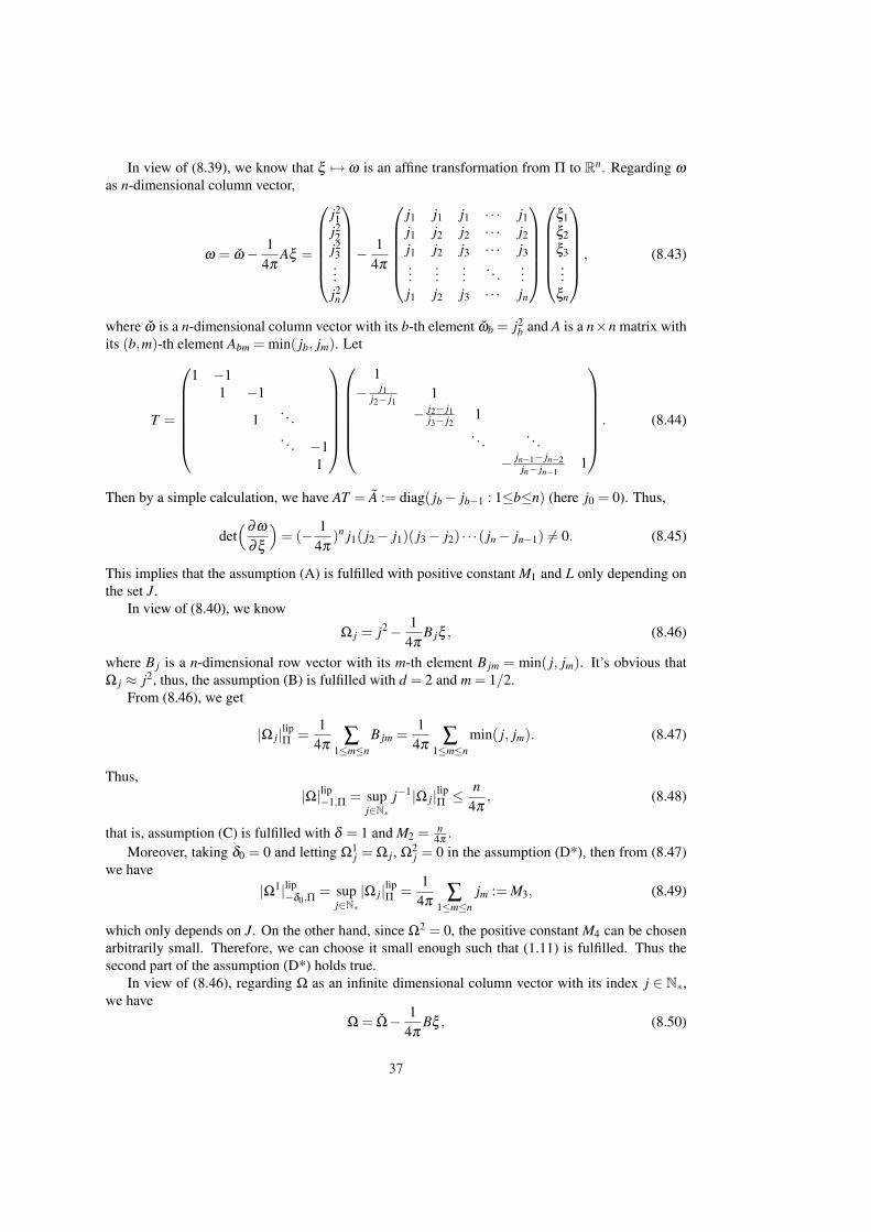
In view of (8.39), we know that ξ 7→ ω is an affine transformation from Π to Rn. Regarding ωas n-dimensional column vector,
This implies that the assumption (A) is fulfilled with positive constant M1 and L only depending onthe set J.
In view of (8.40), we know
Ω j = j2− 14π
B jξ , (8.46)
where B j is a n-dimensional row vector with its m-th element B jm = min( j, jm). It’s obvious thatΩ j ≈ j2, thus, the assumption (B) is fulfilled with d = 2 and m = 1/2.
From (8.46), we get
|Ω j|lipΠ =1
4π ∑1≤m≤n
B jm =1
4π ∑1≤m≤n
min( j, jm). (8.47)
Thus,|Ω|lip−1,Π = sup
j∈N∗j−1|Ω j|lipΠ ≤ n
4π, (8.48)
that is, assumption (C) is fulfilled with δ = 1 and M2 = n4π .
Moreover, taking δ0 = 0 and letting Ω1j = Ω j, Ω2
j = 0 in the assumption (D*), then from (8.47)we have
|Ω1|lip−δ0,Π = supj∈N∗
|Ω j|lipΠ =1
4π ∑1≤m≤n
jm := M3, (8.49)
which only depends on J. On the other hand, since Ω2 = 0, the positive constant M4 can be chosenarbitrarily small. Therefore, we can choose it small enough such that (1.11) is fulfilled. Thus thesecond part of the assumption (D*) holds true.
In view of (8.46), regarding Ω as an infinite dimensional column vector with its index j ∈ N∗,we have
Ω = Ω− 14π
Bξ , (8.50)
37
where Ω is an infinite dimensional column vector with its j-th element Ω j = j2 and B is a ∞× nmatrix with its j-th row B j. For the first part of the assumption (D*), regarding k and l as n-dimensional and infinite dimensional row vectors respectively, we have to check for every k ∈ Zn
and l ∈ Z∞ with 1≤ |l| ≤ 2,
kω + lΩ 6= 0 or kA+ lB 6= 0. (8.51)
By a simple calculation, we have BA−1 = BT A−1 = B, which is a ∞×n matrix with its j-th row B j:
(1) B j = ( jj1
,0, · · · ,0) for j < j1, only the first element nonzero;
(2) B j = (0, · · · ,0,jm+1− j
jm+1− jm, j− jm
jm+1− jm,0, · · · ,0) for jm < j < jm+1 with 1 ≤ m < n, only the m-th
and (m+1)-th elements nonzero;
(3) B j = (0, · · · ,0,1) for j > jn, only the last element nonzero.
Then the second inequality of (8.51) is equivalent to
that for j ∈N1∗⋃N2∗ the nonzero elements of B j are positive and less than 1. Thus the equality (8.52)
holds true for k ∈ Zn and 1≤ |l| ≤ 2 except the following three cases:
(1)
l j = ±2, j = j1/2
0, otherwise , km = ∓1, m = 1
0, otherwise ;
(2) For a fixed m′ with 1≤ m′ < n,
l j = ±2, j = ( jm′ + jm′+1)/2
0, otherwise , km =
∓1, m = m′∓1, m = m′+10, otherwise
;
(3) l j = 0 for j ∈ N1∗⋃N2∗, and
km =
0, 1≤ m < n−∑ j∈N∗ l j, m = n .
It’s easy to check that the first inequality of (8.51) holds true for all of the above three cases. There-fore, the first part of the assumption (D*) holds true.
Now we consider sup norm and Lipschitz semi-norm of the perturbation
P = Q+R+ εK (8.53)
on D(s,r)×Π, where D(s,r) is defined in (1.2) by letting p = N + 1/2 and Π is defined in (8.42).We choose s > 0 a constant, and
r = ε1/4. (8.54)
In view of (8.41), we have
‖XQ‖r,a,p−1,D(s,r)×Π = O(r2) = O(ε1/2). (8.55)
38
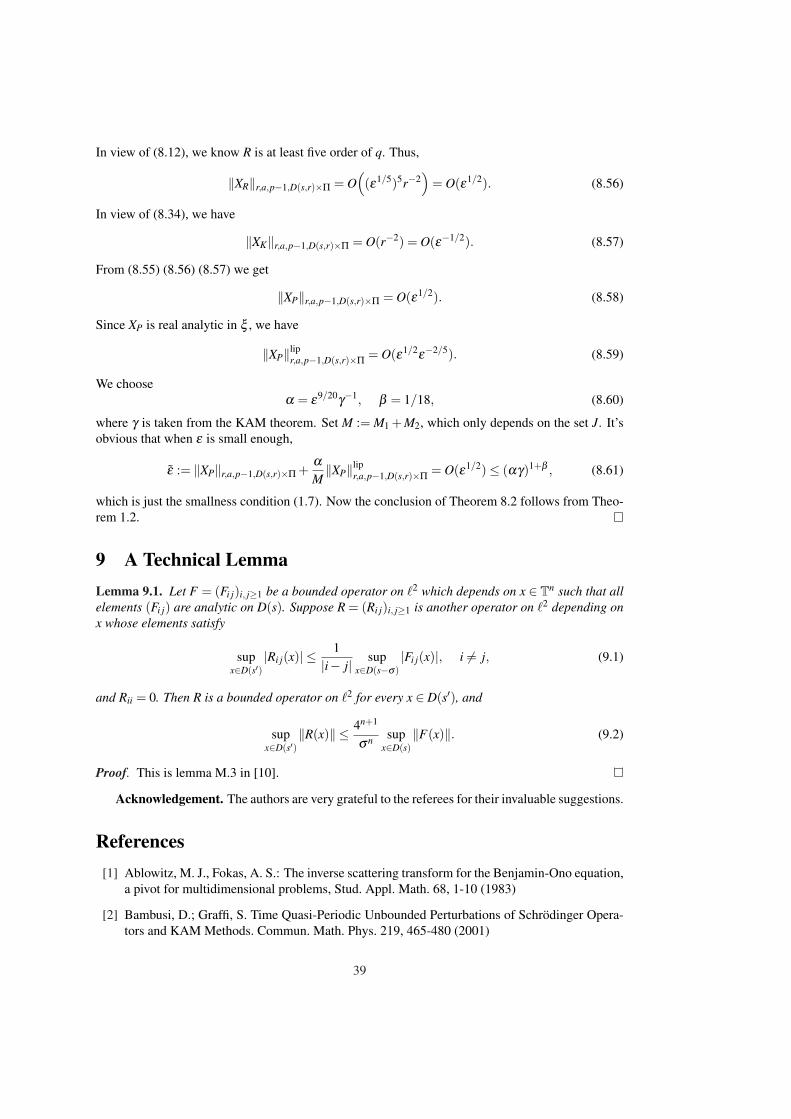
In view of (8.12), we know R is at least five order of q. Thus,
‖XR‖r,a,p−1,D(s,r)×Π = O((ε1/5)5r−2
)= O(ε1/2). (8.56)
In view of (8.34), we have
‖XK‖r,a,p−1,D(s,r)×Π = O(r−2) = O(ε−1/2). (8.57)
From (8.55) (8.56) (8.57) we get
‖XP‖r,a,p−1,D(s,r)×Π = O(ε1/2). (8.58)
Since XP is real analytic in ξ , we have
‖XP‖lipr,a,p−1,D(s,r)×Π = O(ε1/2ε−2/5). (8.59)
We chooseα = ε9/20γ−1, β = 1/18, (8.60)
where γ is taken from the KAM theorem. Set M := M1 +M2, which only depends on the set J. It’sobvious that when ε is small enough,
ε := ‖XP‖r,a,p−1,D(s,r)×Π +αM‖XP‖lip
r,a,p−1,D(s,r)×Π = O(ε1/2)≤ (αγ)1+β , (8.61)
which is just the smallness condition (1.7). Now the conclusion of Theorem 8.2 follows from Theo-rem 1.2.
9 A Technical LemmaLemma 9.1. Let F = (Fi j)i, j≥1 be a bounded operator on `2 which depends on x ∈ Tn such that allelements (Fi j) are analytic on D(s). Suppose R = (Ri j)i, j≥1 is another operator on `2 depending onx whose elements satisfy
supx∈D(s′)
|Ri j(x)| ≤ 1|i− j| sup
x∈D(s−σ)|Fi j(x)|, i 6= j, (9.1)
and Rii = 0. Then R is a bounded operator on `2 for every x ∈ D(s′), and
supx∈D(s′)
‖R(x)‖ ≤ 4n+1
σn supx∈D(s)
‖F(x)‖. (9.2)
Proof. This is lemma M.3 in [10].
Acknowledgement. The authors are very grateful to the referees for their invaluable suggestions.
References[1] Ablowitz, M. J., Fokas, A. S.: The inverse scattering transform for the Benjamin-Ono equation,
a pivot for multidimensional problems, Stud. Appl. Math. 68, 1-10 (1983)
[2] Bambusi, D.; Graffi, S. Time Quasi-Periodic Unbounded Perturbations of Schrodinger Opera-tors and KAM Methods. Commun. Math. Phys. 219, 465-480 (2001)
39
[3] Benjamin, T. B.: Internal waves of permanent form in fluids of great depth. J. Fluid Mech. 29,559-592 (1967)
[4] Bourgain, J.: Recent progress on quasi-periodic lattice Schrodinger operators and HamiltonianPDEs. Russian Math. Surveys 59(2), 231-246 (2004)
[5] Klainerman, S.: Long-time behaviour of solutions to nonlinear wave equations. In Proceedingsof International Congress of Mathematics (Warsaw), 1209-1215 (1983)
[6] Kuksin, S. B.: On small-denominators equations with large varible coefficients. J. Appl. Math.Phys.(ZAMP) 48, 262-271 (1997)
[7] Kuksin, S. B.: Analysis of Hamiltonian PDEs, Oxford Univ. Press, Oxford, 2000
[8] Kuksin, S. B.: Fifteen years of KAM in PDE, “Geometry, topology, and mathematical physics”:S. P. Novikov’s seminar 2002-2003 edited by V. M. Buchstaber, I. M. Krichever. Amer. Math.Soc. Transl. Series 2, Vol.212, 2004, pp.237-257
[9] Kuksin, S. B., Poschel, J: Invariant Cantor manifolds of quasi-periodic oscillations for a non-linear Schrodinger equation. Ann. Math. 143, 147-179 (1996)
[10] Kappeler, T., Poschel, J.: KdV&KAM. Springer-Verlag, Berlin Heidelberg, 2003
[11] Lax, P. D.: Development of singularities of solutions of nonlinear hyperbolic partial differentialequations. J. Math. Phys. 5, 611-613 (1964)
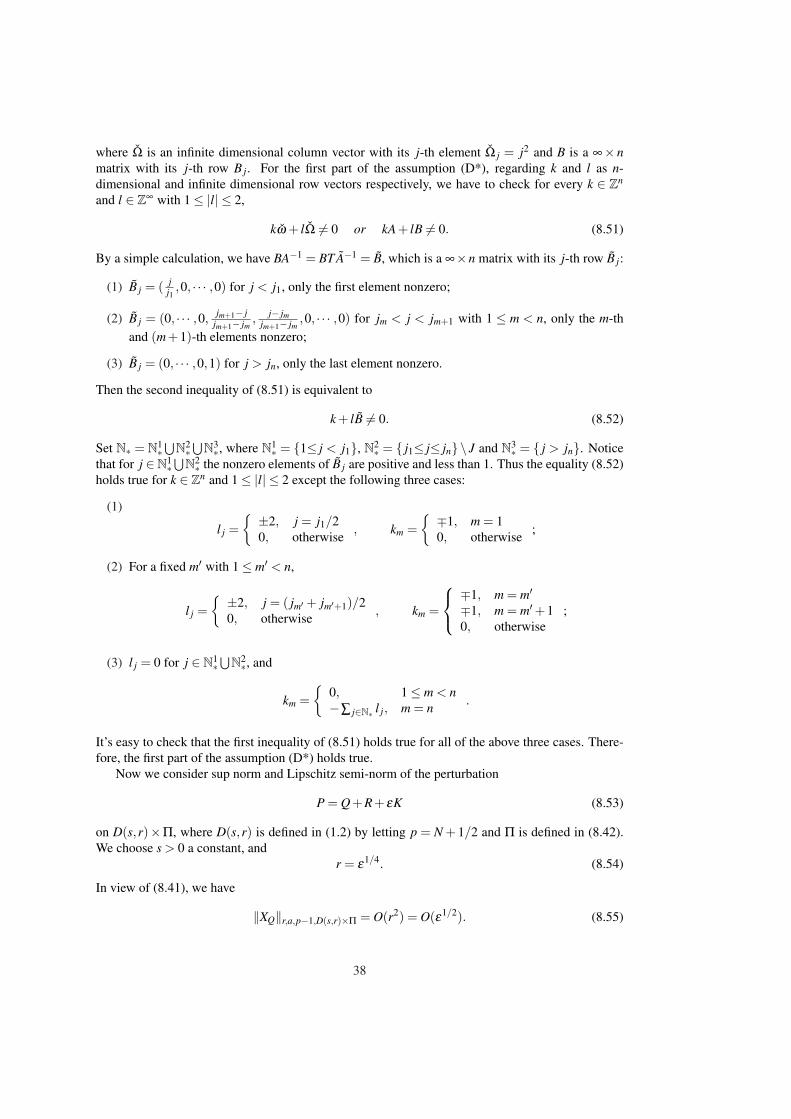


![web.ma.utexas.edu · OrqS T%S hX]cJwN:V3[0V WXT-N*L*\X[NwS3[0VK_ YX\QN*J0L µ S T-T*Z"TxN:JMz YXL-V,Vbn V nqN*PXJeJ ,Z"T-N*J0WX[MJeV n`S~L*JMWXVKL-_eS ]cZ"f0SbN:ZcVKW |Q ,J0zÆY&VKZ"W/N](https://static.documents.pub/doc/80x56/5f646da9258dc735a00c05c4/webma-orqs-ts-hxcjwnv30v-wxt-nlxnws30vk-yxqnj0l-s-t-tztxnjmz.jpg)
