Page 1
1
T H E U N I V E R S I T Y O F T U L S A
THE GRADUATE SCHOOL
HORIZONTAL PIPE SEPARATOR (HPS©)
EXPERIMENTS AND MODELING
by Ciro Andrés Pérez
A dissertation submitted in partial fulfillment of
the requirements for the degree of Doctor of Philosophy
in the Discipline of Petroleum Engineering
The Graduate School
The University of Tulsa
2005
Page 3
iii
ABSTRACT
Pérez, Ciro A. (Doctor of Philosophy in Petroleum Engineering).
Horizontal Pipe Separator (HPS©). Experiments and modeling
Directed by Professors Ovadia Shoham and Ram S. Mohan (205 pp., Chapter 6)
(329 words)
The objective of this study is to investigate experimentally and theoretically the
developing region of oil-water flow in horizontal pipes. The study aims at using the
developing region of the pipe as an oil-water separator (Horizontal Pipe Separator,
HPS©).
An experimental HPS© facility has been designed and constructed, to enable
measurements of local parameters in oil-water flow in the developing region of the flow
in a 3.75-in.-ID 19.33-ft-long acrylic pipe. Special instrumentation was developed for
acquiring the local parameters data, namely, local velocity profiles; water cut profiles and
droplet size distribution. Experimental data were acquired for mixture velocities of 0.44
and 0.58 ft/s, and water cuts of 10, 30, 50 and 70%, measured at two metering stations,
located at 7.5 ft and 13.5 ft from the inlet, respectively. The data were acquired for a
concentric inlet with and without a mixer, and for three different outlet configurations.
Also, inlet flowrates as well as the water cut in both the oil and water outlet were
Page 4
iv
measured as functions of the split ratio. For all experimental runs, the flow did not reach
fully developed flow conditions.
A model is developed for the prediction of the flow evolution in the developing
region of the HPS©. The model comprises two sub-models: one-dimensional flow of
three layers (hydrodynamic sub-model) and population balance coalescence theory
(coalescence sub-model). The three layers are, from top to bottom (for water-continuous
flow at the inlet): pure oil, packed dispersion of oil in water and loose dispersion of oil in
water. For oil-continuous flow the three layers are loose dispersion of water in oil, packed
dispersion of water in oil and clear water. Linear velocity and water cut profiles were
assumed for the intermediate (packed dispersion) layer. Average and minimum water cut
of the intermediate (packed dispersion) layer are required as input. The results of the
model match fairly well the experimental data, with respect to layer height development;
velocity and water cut profiles and overall droplet size distributions.
Page 5
v
ACKNOWLEDGEMENTS
I really want to give my deepest gratitude to my advisor, Dr. Ovadia Shoham, for
his support and confidence during the development of this study. I also want to thank Dr.
Ram Mohan, my co-advisor for his help and reviews during the different phases of this
study. Thanks are due also to Dr. Luis Gómez, Dr. Shoubo Wang and Dr. Gene Kouba,
for their valuable suggestions and support. I am very grateful to The University of Tulsa,
and to the Tulsa University Separation Technology Project (TUSTP) for the financial
support and opportunity to accomplish this endeavor. I would like to thank all the TUSTP
members and graduate students for the time we invested sharing ideas, and for the
friendship they showed during this time, especially to Dr. Nólides Guzman, Mr. Carlos
Avila and Dr. Carlos Torres. I am especially grateful to Mrs. Judy Teal for her help, and
to Oscar Escobar and Rafael Rivas. Thanks to Marisabel Herrera, Jose Alaña, Mariela
Lander, and all the people that made this whole experience richer. Also, thanks are due to
the “LABCEM” Laboratory (specially to Nathaly Moreno, Andrés Tremante and Frank
Kenyery) and to the “Departamento de Termodinamica y Fenomenos de Transporte”,
both at the Universidad Simón Bolívar, in Caracas, Venezuela, for all the help they gave
me to accomplish this milestone. Finally, all my gratitude to my family, that helped me so
much. I would like to dedicate this work to m y parents Benigno and Fidela, my sisters
Maria Eglee, Carmen Alicia and Simone, and my brother Pedro.
Page 6
vi
TABLE OF CONTENTS
Page
ABSTRACT....................................................................................................................... iii ACKNOWLEDGEMENTS.................................................................................................v TABLE OF CONTENTS................................................................................................... vi LIST OF TABLES............................................................................................................. ix LIST OF FIGURES .............................................................................................................x CHAPTER 1: INTRODUCTION ......................................................................................1 CHAPTER 2: LITERATURE REVIEW ..........................................................................4 2.1 Two-Phase Fully Developed Liquid-Liquid Flow .........................................4 2.1.1 Flow Patterns ......................................................................................5 Flow Patterns Classification and Flow Pattern Maps ......................7 Flow Pattern Prediction..................................................................15 2.1.2 Pressure Drop ...................................................................................18 2.2 Liquid-Liquid Developing Flow Region.......................................................19 2.2.1 Effects of Inline Mixing .....................................................................21 2.2.2 Effect of Pre-Mixing ..........................................................................21 2.3 Measurement of Local Parameters in Oil-Water Flow ..............................23 2.3.1 Velocity..............................................................................................23 2.3.2 Local Holdup.....................................................................................23 2.3.3 Local Droplet Size Distribution ........................................................24 2.3.4 Local Continuous Phase Measurement.............................................24 2.4 Coalescence/Breakup and Droplet Size Distribution..................................24 2.4.1 Droplet Coalescence .........................................................................25 2.4.2 Droplet Breakup................................................................................30 2.4.3 Probability Density Functions ..........................................................30 Continuous-Size Distribution.........................................................31 2.4.4 Sauter Mean Diameter ......................................................................33 2.5 Outlet Studies in Horizontal Pipes ...............................................................34 2.6 Use of Horizontal Pipes as Separators .........................................................35
Page 7
vii
CHAPTER 3: EXPERIMENTAL PROGRAM .............................................................36 3.1 Experimental Facility ....................................................................................36 3.1.1 Storage and Metering Section ...........................................................37 3.1.2 Test Section .......................................................................................39 3.1.3 Local Measurement Instrumentation ................................................43 3.1.4 Gas-Oil-Water Separation Section ...................................................45 3.1.5 Data Acquisition System ...................................................................46 3.1.6 Working Fluids..................................................................................47 3.2 Experimental Test Matrix .............................................................................49 3.2.1 Velocity Profiles at Vertical Plane, and Velocity Surfaces ...............50 3.2.2 Water Cut Profiles.............................................................................54 3.2.3 Layer Height......................................................................................57 3.2.4 Droplet Size Distribution Profiles.....................................................58 3.2.5 Pressure Drop ...................................................................................67 3.2.6 Outlets Performance .........................................................................70 CHAPTER 4: MODELING..............................................................................................74 4.1 Hydraulic Sub-Model ....................................................................................74 4.1.1 Number of Layers ..............................................................................74 4.1.2 Layer Mixture Properties ..................................................................77 4.1.3 Mathematical Formulation ...............................................................79 Taitel et. al. (1995) 3-layered model..............................................79 4.2 Coalescence Sub-Model .................................................................................85 4.2.1 Physical Phenomena .........................................................................85 4.2.2 Assumptions.......................................................................................87 4.2.3 Mathematical Formulation ...............................................................88 Estimation of the number of collisions per unit volume per unit time .........................................................................................88 Estimation of the number of coalescing collisions per unit volume per unit time ......................................................................89 4.3 Closure Rules..................................................................................................91 4.3.1 Estimation of the Settling Velocity ....................................................91 4.3.2 Estimation of the Velocity and Water Cut Profiles in the Packed Layer ....................................................................................92 4.3.3 Estimation of the Local Droplet Size Distribution in the Packed Layer ....................................................................................98 Evolution of the Local Distribution Parameters Along the Separator ......................................................................................106 4.3.4 Coalescence Estimation Procedure ................................................106 4.4 Calculation Procedure .................................................................................108 CHAPTER 5: RESULTS AND DISCUSSION .............................................................111 5.1 Comparison of Layers Height Evolution ...................................................111
Page 8
viii
5.2 Comparison of Velocity and Water Cut Profiles ......................................115 5.3 Comparison of Droplet Size Distribution Evolution in Packed Layer....119 5.4 Comparison of Droplet Size Distribution as a Function of the Height in Packed Layer...........................................................................................123 CHAPTER 6: CONCLUSIONS AND RECOMMENDATIONS ...............................129 NOMENCLATURE ........................................................................................................134 REFERENCES ................................................................................................................138 APPENDIX I: LOCAL MEASUREMENT SYSTEMS............................................145 APPENDIX II: LAYER HEIGHT COMPARISON BETWEEN LOCAL WATER CUT AND PHOTOGRAPHIC METHODS MEASUREMENTS .......................................................176 APPENDIX III: LOCAL VELOCITY MEASUREMENT .........................................180 APPENDIX IV: CALCULATION OF THE VELOCITY AND WATER CUT SLOPES FOR LINEAL VELOCITY PROFILE APPROXIMATION ...........................................................................197 APPENDIX V: DROPLET SIZE MEASUREMENT ................................................205
Page 9
ix
LIST OF TABLES
Table 2.1 Classification of Gas-Liquid Flow Patterns (Ishii, 1975) ................................. 14
Table 2.2 Classification of Liquid-Liquid Flow Patterns (Kurban, 1997)........................ 14 Table 3.1 Properties of Water-Phase ................................................................................ 47
Table 3.2 Properties of Oil-Phase ..................................................................................... 48
Table 3.3 Average WC in Packed Dispersion Layer (7.5 ft and 13.5 ft).......................... 55
Table 3.4 Average WC in Loose Dispersion Layer (7.5 ft and 13.5 ft)............................ 55
Table 3.5 Dimensionless (h/D) Height of Packed Dispersion Layer-Loose Dispersion
Layer Boundary (7.5 ft) ........................................................................................... 57
Table 3.6 Dimensionless (h/D) Height of Packed Dispersion Layer-Loose Dispersion
Layer Boundary (13.5 ft) .......................................................................................... 57
Table 3.7 Log-Normal Distribution Fitting Parameters for Cumulative Distributions
in Figure 3.21 ............................................................................................................ 65
Table 3.8 Log-Normal Distribution Fitting Parameters for Cumulative Distributions
in Figure 3.22 ............................................................................................................ 65
Table 5.1 Values of b Used to Adjust the Local Droplet Size Distribution in Model ....124
Page 10
x
LIST OF FIGURES
Page
Figure 2.1 Relative Location of Flow Patterns for Light Oil (μO<20 cP) and Water Flow
With Same Density in a Mandhane (1947) Flow Pattern Map. (from Charles et al.,
1961) ........................................................................................................................... 8
Figure 2.2 Relative Location of Flow Patterns for Oil (65 cP) and Water Flow With Same
Density in a Mandhane Flow Pattern Map (From Charles et al., 1961)..................... 8
Figure 2.3 Flow Pattern Map for Water and Oil Flow, With Oil Viscosity of 21.7 mPa*s
in a 39.4 mm ID Pipe. (after Guzhov et al., 1973) ................................................... 10
Figure 2.4 Horizontal Oil-Water Flow Patterns. (after Trallero, 1995)............................ 10
Figure 2.5 Experimental Flow Pattern Map Using Superficial Velocities as Coordinates
(after Trallero, 1995)................................................................................................. 12
Figure 2.6 Experimental Flow Pattern Map Using Mixture Velocity and Input Water Cut
as Coordinates (after Trallero, 1995) ........................................................................ 12
Figure 2.7 ZNS and ZRC Transition Boundaries ............................................................. 17
Figure 2.8 Stratified-Stratified Dispersed Flow Boundary ............................................... 17
Figure 2.9 Schematic of Trallero (1995) Inlet Mixer ....................................................... 20 Figure 3.1 Experimental Facility ...................................................................................... 38
Figure 3.2 Storage and Metering Section ......................................................................... 39
Figure 3.3 HPS© Test Section........................................................................................... 39
Figure 3.4 HPS© Inlet Section .......................................................................................... 40
Page 11
xi
Figure 3.5 KOMAXTM Static Mixer Spool Upstream of the Inlet Section....................... 41
Figure 3.6 HPS© Outlet Configurations............................................................................ 41
Figure 3.7 Location of Local Measurement Ports and Pressure Tap Ports....................... 42
Figure 3.8 Experimental Test Matrix Shown on Steady State Flow Pattern Map........... 49
Figure 3.9 Velocity Profiles at Vertical Plane (vM=0.44 ft/s) ........................................... 51
Figure 3.10 Velocity Profiles at Vertical Plane (vM=0.58 ft/s) ......................................... 51
Figure 3.11 Velocity Contours at 7.5 ft from Inlet (vM=0.44 ft/s) .................................... 52
Figure 3.12 Velocity Contours at 13.5 ft from Inlet (vM=0.44 ft/s) .................................. 52
Figure 3.13 Velocity Contours at 7.5 ft from Inlet. (vM=0.58 ft/s)................................... 53
Figure 3.14 Velocity Contours at 13.5 ft. from Inlet. (vM=0.58 ft/s)................................ 53
Figure 3.15 Water Cut Profiles at Vertical Plane (vM=0.44 ft/s) ...................................... 56
Figure 3.16 Water Cut Profiles at the Vertical Plane. (vM=0.58 ft/s) ............................... 56
Figure 3.17 Droplet Size Distribution Profiles at Vertical Plane (vM=0.44 ft/s) .............. 59
Figure 3.18 Droplet Size Distribution Profiles at Vertical Plane (vM=0.58 ft/s) .............. 60
Figure 3.19 d32 Profiles at Vertical Plane (vM=0.44 ft/s) .................................................. 61
Figure 3.20 d32 Profiles at Vertical Plane (vM=0.58 ft/s) .................................................. 61
Figure 3.21 Overall Droplet Size Distribution in Packed Dispersion Layer (vM=0.44 ft/s)
................................................................................................................................... 63
Figure 3.22 Overall Droplet size Distribution in Packed Dispersion Layer (vM=0.58 ft/s)
................................................................................................................................... 64
Figure 3.23 Pressure Drop Along HPS© for Different Water Cuts, Without Mixer......... 69
Figure 3.24 Pressure Drop Along HPS©, With Mixer ...................................................... 69
Figure 3.25 Oil Cut at Oil Outlet (vM=0.44 ft/s) ............................................................... 72
Page 12
xii
Figure 3.26 Oil Cut at Oil Outlet (vM=0.58 ft/s) ............................................................... 73 Figure 4.1 Three Layer Developing Flow. (vM=0.44 ft/s, 50% WC, without Mixer, 14 ft
from Inlet) ................................................................................................................. 75
Figure 4.2 Force Balances Over Each of the Three Layers. (after Taitel et. al., 1995).... 80
Figure 4.3 Coalescence in Simple Shear Flow due to Velocity Gradient......................... 86
Figure 4.4 Schematic of Proposed Velocity and WC Profiles in the Packed Dispersion
Layer ......................................................................................................................... 93
Figure 4.5 Cumulative Frecuency of Selected Droplet Diameters as Function of Height
Inside the HPS© (70%WC, vM=0.44 ft/s, w/mixer, 7.5 ft from the inlet) ................. 99
Figure 4.6 Cumulative Frequency of Selected Droplet Diameters as Function of Height
Inside the HPS© (70%WC, vM=0.58 ft/s, w/mixer, 7.5 ft from the inlet) ................. 99
Figure 4.7 Procedure of Assignment of Local Droplet Size Distributions as Function of
Height (nb=5).......................................................................................................... 104
Figure 4.8 Calculation Procedure Flowchart .................................................................. 110
Figure 5.1. Comparison of Model Predictions and Experimental Data for Layer Heights
Evolution (vM=0.44 ft/s)..........................................................................................113
Figure 5.2. Comparison of Model Predictions and Experimental Data for Layer Heights
Evolution (vM=0.58 ft/s).......................................................................................... 114
Figure 5.3 Comparison of Model Predictions and Experimental Data for 30% WC.
Mixture Velocities vM=0.44 and 0.58 ft/s ............................................................... 116
Figure 5.4 Comparison of Model Predictions and Experimental Data for 50% WC.
Mixture Velocities vM=0.44 and 0.58 ft/s ............................................................... 117
Page 13
xiii
Figure 5.5 Comparison of Model Predictions and Experimental Data for 70% WC. Mix.
Velocities vM=0.44 (a) and 0.58 (b) ft/s .................................................................. 118
Figure 5.6. Comparison of Model Predictions and Experimental Data for Droplet Size
Distribution Change between Metering Stations (vM=0.44 ft/s) ............................. 120
Figure 5.7 Comparison of Model Predictions and Experimental Data for Droplet Size
Distribution Change between Metering Stations (vM=0.58 ft/s) ............................. 121
Figure 5.8 Comparison of Model Adjusted and Experimental Measured Droplet Size
Distributions at 7.5 ft from Inlet, vM=0.44 ft/s........................................................ 125
Figure 5.9 Comparison of Model Adjusted and Experimental Measured Droplet Size
Distributions at 7.5 ft from Inlet, vM=0.58 ft/s........................................................ 126
Figure 5.10 Comparison of Model and Experimental Measured Droplet Size
Distributions at 13.5 ft from Inlet, vM=0.44 ft/s...................................................... 127
Figure 5.11 Comparison of Model and Experimental Measured Droplet Size
Distributions at 13.5 ft from Inlet, vM=0.58 ft/s...................................................... 128
Page 14
1
CHAPTER 1
INTRODUCTION
The actual world’s energy demand requires further advances in the knowledge of
the generation, production and development of proven and new energy sources. To this
end, the nuclear industry, and more recently the petroleum industry, have been driven to
study the flow of two or three phases through production and processing facilities. These
studies are aimed at the challenges of defining the flow pattern, pressure gradient, phase
volume fractions and separation efficiency of these multiphase flows.
As the need for energy production increases, the requirement of production of
more energy at lower costs is pursued. The gained knowledge of the flowing phenomena
in multiphase flow enables optimization of the different components of the entire
production and processing infrastructure.
The requirements of oil-water separation in more challenging environments,
especially in sub-sea production, give rise to the need of alternative separation
technologies that can decrease deployment expenses, and increase the robustness of the
energy production process.
Page 15
2
The natural segregation of crude oil and water due to density difference can occur
not only in gravity based vessel-type separators (widely used by the petroleum industry),
where the fluids have large residence time, but also when flowing through pipes, if the
flowing conditions are favorable for flow segregation.
Thus, the use of pipes as separators is especially suitable for sub-sea applications.
The ease of installation and simplicity of operation of pipe separators ensure reliable
performance of the entire production system. The proposed Horizontal Pipe Separator
(HPS©)1 is a simple concept: a pipe spool with appropriate geometry promoting natural
separation of the phases under favorable flow conditions. However, not many studies
have been published on HPS©, especially addressing the developing flow along it. Thus,
the objectives of this study are:
1- Study the behavior of oil-water mixtures in horizontal pipes;
2- Develop a mechanistic model that predicts separation efficiency for given fluids,
geometry and flow rates;
3- Compare/refine the model with data obtained in this study and from literature;
4- Develop a computational code based on the developed model..
This dissertation is divided into six chapters. Chapter 1, the current one, is this
introduction. The description of the following five chapters follows:
1 HPS© – Horizontal Pipe Separator – Copyright, The University of Tulsa, 1999
Page 16
3
Chapter 2 presents a literature review on the topics related to oil-water flow in
pipes and to droplet coalescence mechanisms. Chapter 3 gives a description of the
experimental facility, the instrumentation used, the experimental matrix and testing
procedures; finally the measured data are presented. Chapter 4 provides details of the
proposed model for the prediction of the flow evolution in the developing region of the
HPS©. A comparison between the model predictions and the experimental data is given in
Chapter 5, along with the discussion of the results. Finally, Chapter 6 provides the
conclusions and the recommendations.
Page 17
4
CHAPTER 2
LITERATURE REVIEW
There is a limited availability of experimental data for liquid-liquid flow (as
compared to gas-liquid flow), despite two peaks in the rate of publication of liquid-liquid
studies: the first peak occurred in the early 1960's (Charles et al., 1961; etc.), and the
second in the past 10 years. Still today, many of published models for liquid-liquid flows
represent extensions of gas-liquid models rather than an original methodology.
This chapter presents literature review on liquid-liquid oil-water flow phenomena
in pipes as follows: (1) Fully developed liquid-liquid flow; (2) Liquid-liquid developing
flow region; (3) Measurement of local parameters in oil-water flows; (4)
Coalescence/break up and droplet size distributions; (5) Outlets studies in horizontal
pipes; and (6) Use of horizontal pipes as separators.
2.1 Two Phase Fully Developed Liquid-Liquid Flow
This section presents previously published studies on fully developed liquid-
liquid flow, including flow pattern definitions and pressure drop phenomena.
Page 18
5
2.1.1 Flow Patterns
In two-phase flow in pipes, the deformable interface between the immiscible
phases can exist in different shapes or spatial distributions for different flow conditions.
These configurations are commonly called flow patterns.
For gas–liquid systems, the flow patterns are considered as functions of the
following variables (Shoham, 2006): (a) operational parameters, namely, the gas and
liquid flowrates, (b) geometrical variables, including pipe diameter and inclination angle,
and (c) the physical properties of the two phases, i.e., gas and liquid densities, viscosities
and the surface tension. These same parameters are thought to control the flow pattern
phenomena for liquid-liquid mixtures flowing in pipes (i.e., Trallero, 1995; Kurban,
1997). More recent studies such as Angeli (1996), Soleimani (1999) and Shi (2001)
suggested that the flow pattern configuration is also a function of the pipe material, and
of the presence of additional components (such as surfactants) in the mixture. Most of
these studies were executed on small-diameter pipes, namely, 1-inch and 2-inch nominal
diameters.
These flow patterns are usually presented in the form of two-dimensional plots,
or flow pattern maps. The importance of the flow pattern maps is that within each pattern
the flow has certain similar hydrodynamic characteristics. The knowledge of these
characteristics simplifies the problem of building a hydrodynamic flow model for the
Page 19
6
phenomena into the construction of hydrodynamic sub-models appropriate for each flow
pattern.
In order to differentiate between the different flow patterns, several different
methods have been developed and applied for gas-liquid and liquid-liquid flow pattern
detection.
Visual observation is one of the most common methods to identify flow patterns
in multiphase flow. The identification is done by using a photographic/video technique to
view the flow through the wall of a transparent tube. High-speed photography must be
used to capture the flow patterns at high fluid mixture velocities. However, the
disadvantage of the visual observation method is the difficulty to observe the internal
structure of the flow clearly (Hewitt et al., 1997). This problem can be mitigated by other
visualization alternatives such as X-ray photography.
Since photographic methods are somewhat subjective and not generally reliable,
more objective and quantitative detection methods have been developed. Conductivity
probes (Angeli, 1996; and Trallero, 1995) provide a more precise method of
investigating the spatial distribution of two phases across the cross section of the tube
(Angeli and Hewitt 1998). Valle and Kvandal (1995) used local sampling to measure the
liquid fraction at points across the cross section of a pipeline. Gamma ray densitometers
(Elseth, 2001), and High Frequency Impedance Probes (Lovick 2004) are other devices
used for measuring the local distribution of two phases. All of these alternative tech-
Page 20
7
niques provide valuable additional information for defining flow patterns in a more
objective way.
Flow Patterns Classification and Flow Pattern Maps
From the initial studies of Russel et al. (1959), Russel & Charles (1959), Charles
et al. (1961) and Charles & Redberger (1962), different but related flow patterns had
been defined. Charles et al. (1961) observed the flow patterns that occurred during the
flow of equal density oil and water mixture in a horizontal, 1-inch ID cellulose acetate
butyrate pipe. Three oils with dynamic viscosities of 6.29, 16.8 and 65 mPa*s were used.
A schematic of the resulting flow pattern maps plotted in terms of the superficial
velocities of the two liquids, are shown in Figure 2.1 for the two lighter oils and in Figure
2.2 for the heavier one. The following flow patterns were defined in this work:(a) Water
droplets in oil, (b) Water bubbles in oil, (c) Oil in water concentric flow, (d) Water slugs
in oil, (e) Oil slugs in water, (f) Oil bubbles in water and (g) Oil droplets in water. It
should be noted that the absence of density difference between the two liquids resulted in
a symmetric flow about the pipe axis. Thus, the stratified flow pattern was not observed.
The flow patterns for the 6.29 and 16.8 mPa*s viscosity oils (Figure 2.1) were almost
identical, with only one oil continuous flow pattern. The flow patterns for the heavier oil
(Figure 2.2) were similar to those already observed, except at the low water velocities,
where a succession of different flow patterns with oil as the continuous-phase occurred,
as shown in Figure 2.2. Charles et al. (1961) attributed this difference to the fact that the
most viscous oil wetted the pipe wall more than the other two oils.
Page 21
8
Figure 2.1 Relative Location of Flow Patterns for Light Oil (μO<20 cP) and Water Flow
With Same Density in a Mandhane (1947) Flow Pattern Map. (from Charles et al., 1961)
Figure 2.2 Relative Location of Flow Patterns for Oil (65 cP) and Water Flow With Same
Density in a Mandhane Flow Pattern Map. (From Charles et al., 1961)
0.01
0.1
1.0
10. Water droplets in oil
Oil in water concentric
Oil slugs in water
Oil bubbles in water
Oil drops in water
Superficial water velocity [ft/s]
Supe
rfic
ial o
il ve
loci
ty [f
t/s]
0.05 0.1 1.0 10.
Water drops in oil
Oil in water concentric
Oil slugs in water
Oil bubbles in water
Oil drops in water
Superficial water velocity [ft/s]
Supe
rfic
ial o
il ve
loci
ty [f
t/s]
Water slugs in oil
Water bubbles in oil
0.01
0.1
1.0
10
0.05 0.1 1.0 10.
Page 22
9
Russell et al. (1959), working in a similar pipe with water and oil (viscosity 18
mPa*s and density 834 kg/m3), observed similar flow patterns to those reported by
Charles et al. (1961) but with the asymmetry imposed by the density difference. The
annular flow pattern did not occur at all, while for a wide range of velocities the stratified
flow pattern was present.
Using similar flow pattern classifications to the ones used by Charles et al.
(1961), other flow pattern maps for horizontal flow of oil and water were developed, but
with mixture velocity and water volume fraction as axes. For example, Guzhov et al.
(1973) presented such a flow pattern map, for water and oil with oil viscosity of 21.7
mPa*s and density 896 kg/m3 at 20°C in a horizontal, 39.4 mm ID pipe, which schematic
is shown in Figure 2.3. Also, Arirachakaran et al. (1989) published a similar map for
water and oil, with oil viscosity of 84 mPa*s at 21°C in a 39.3 mm ID pipe.
Since these studies, experimental and phenomenological models have evolved,
and slightly different flow pattern classifications have been presented. There have been a
convergence on similar classifications during the last ten years, as can be seen in the
following examples: Trallero (1995), Nadler and Mewes (1997), and Kurban (1997).
Trallero (1995) acquired experimental data in a two 2-inch nominal 51-ft-long
pipe facility, connected with a U bend. Experimental fluids were mineral oil (Cristex AF-
M 31) and tap water, with density ratio of 0.85, viscosity ratio of 29, and interfacial
tension of 36 dynes/cm (at 78º F).
Page 23
10
Figure 2.3 Flow Pattern Map for Water and Oil Flow, With Oil Viscosity of 21.7 mPa*s
in a 39.4 mm ID Pipe. (after Guzhov et al., 1973)
Figure 2.4 Horizontal Oil-Water Flow Patterns (after Trallero, 1995)
Stratified Flow
Water drops and oil layer
Oil drops
Water drops
Intermittent flow
Oil drops and water layer
0 0.5 1. Volume fraction of water
Mix
ture
vel
ocity
[m/s
]
1.
2.
3.
Page 24
11
The author proposes a flow pattern classification for oil-water flows where six
flow patterns were identified and classified into two categories:
(1) "segregated" flow with two sub-regimes of stratified and stratified with
mixing at the interface;
(2) "dispersed" flow with two sub-regimes of water dominated dispersed flow and
oil dominated dispersed flow.
Figure 2.4 shows the “segregated” flow patterns (on the left hand side), and the
“dispersed” flow patterns (on the right hand side). The author presents the experimental
results using both the Charles et al. (1961) (Figure 2.5) and Guzov et al. (1973) (Figure
2.6) coordinate systems for the flow pattern maps.
Nadler and Mewes (1997) presented a slightly different classification of flow
patterns (the authors added an extra flow pattern: dispersion of water in oil-dispersion of
oil in water-pure water flow pattern). Their facility consisted of a 48-m-long, 59-mm (2.3
inch)-ID test section. Mineral oil and tap water were used, with a density ratio of 0.85,
and a viscosity ratio from 28 to 35, in the range of 18ºC to 30ºC. They plotted their
results in both flow pattern map types.
Page 25
12
Figure 2.5 Experimental Flow Pattern Map Using Superficial Velocities as Coordinates
(after Trallero, 1995)
Figure 2.6 Experimental Flow Pattern Map Using Mixture Velocity and Input Water Cut
as Coordinates (after Trallero, 1995)
Page 26
13
Finally, Kurban (1997) presented a flow pattern classification based on the study
of Ishii (1975) for gas-liquid flows. Experimental results were acquired using two
facilities: 1) 8-m-long stainless steel and acrylic pipes of 1-inch nominal diameter, using
EXXSOL D-80 mineral oil and tap water (oil-water density Ratio 0.8, viscosity ratio
1.6, interfacial tension 0.017 N/m, operating temperature 25ºC), and 2) 42-m-long, 77.90-
mm (3 inches) diameter, stainless steel pipe, using water and Shell TELLUS 22 mineral
oil (Density Ratio 0.865, viscosity ratio 45, with no interfacial tension nor operating
temperature reported).
The work of Ishii (1975) provides a classification of two-phase gas-liquid flows
based on the interfacial structures and topology of each phase. The three main categories
were separated flows, mixed or transition flows and dispersed flows, as shown in Table
2.1.
Kurban combined the categories of Ishii (1975), with the experimental
observations obtained from the Imperial College TOWER and WASP rigs (Kurban,
1997) and those reported by Guzhov et al. (1973), Oglesby (1979) and Arirachakaran et
al. (1989), as given by Table 2.2. Kurban (1997) proposes that although the phases for all
the studies were oil and water, such classifications should be valid for any two-phase
flow of two immiscible liquids. He presented his results in terms of dimensionless
variables (namely the generalized Lockhart-Martinelli parameter, non-dimensional wall
Page 27
14
Table 2.1
Classification of Gas-Liquid Flow Patterns (Ishii, 1975)
Category Flow Regime Configuration
Stratified Liquid layer below gas with a planar interface
Separated
Annular Gas core and liquid film
Slug Gas pockets in liquid
Mixed or transition
Annular with Entrainmnent
Gas core with droplets and liquid film with gas bubbles
Bubbly Gas bubbles in liquid continuous phase
Dispersed
Droplet Liquid droplets in gas
Table 2.2
Classification of Liquid-Liquid Flow Patterns (Kurban, 1997)
Category Flow Regime Configuration
Stratified Water layer in oil with a near planar interface
Separated
Core-annular Oil core-water annular film. Circular, and non pipe-concentric interface
Intermittent Phases alternately occupying the pipe as a free and as a dispersed phase
Stratified with dispersion
Layers of a dispersion with a free phase
Mixed or transition
Annular with dispersion
Oil core with water droplets and water film with oil droplets
Water in oil Water droplets in oil continuous phase
Dispersed
Oil in water Oil droplets in water continuous phase
Page 28
15
and interfacial shear stresses and the superficial friction factors) in order to provide
generalization of the results.
Flow Pattern Prediction
Different mechanistic models have been proposed for the prediction of different
flow pattern boundaries. An example is the Brauner and Moalen Maron (1992 a,b)
criteria for the transition from one flow regime to the other, as presented next. In this
model the considered transitions are mainly the boundaries between stratified, annular
and stratified-dispersed flow regimes.
For the stratified flow pattern, Brauner and Moalen Maron (1992 a,b) presented a
temporal stability analysis of the governing continuity and momentum equations and
considered the conditions under which these equations constitute a well-posed initial
value problem. This analysis produces two transition lines, the zero neutral stability
(ZNS) and the zero real characteristics (ZRC) line. These lines are shown in Figure 2.7,
as functions of the superficial velocities of the two phases for a particular oil-water
system. For this case, the upper layer is oil and the lower is water. The authors stated that
the ZNS line represents the transition from stratified-smooth to stratified-wavy flow
pattern, while the ZRC line represents an upper boundary for the existence of the wavy-
stratified configuration, beyond which other flow patterns exist. According to their
analysis the area identified by the ZRC line (corresponding to the stratified flow pattern),
diminishes in size when the density difference between the two phases decreases, the
Page 29
16
viscosity difference between phases increases, and the tube diameter decreases. The
departure from the stratified flow pattern can lead either to annular or stratified-dispersed
flow.
In annular flow, Branuer and Moalen Maron (1992 (b)) assumed a certain ratio of
wall to core phase that can produce large interfacial waves, capable of blocking the core
space and leading to slug flow, and derived an equation for the transition line between
these two regimes. They found that this transition line was not sensitive to fluid
properties and tube diameter.
The stratified-dispersed flow transition on the other hand, may exist as a sub-
division of stratified flow, when one phase flowrate is both considerably smaller than the
other phase flowrate and is flowing in the form of entrained droplets. As a result of
buoyancy forces, these droplets tend to concentrate at the top or the bottom of the pipe,
depending on whether the droplets are lighter or heavier than the continuous phase,
respectively. If the buoyancy force exceeds the surface tension force, the authors
suggested that the droplets will merge together to form a continuous layer.
A transition line based on the equation of the balance of these two forces can then
be derived. One such line for a particular oil-water system is shown in Figure 2.8.
Brauner and Moalen Maron (1992 (b)) analysis showed that a decreasing density or
viscosity difference or an increasing surface tension will result in a larger stratified-
dispersed region. Also, as the tube diameter decreases, the stratified-dispersed flow
pattern is more likely to occur.
Page 30
17
Figure 2.7 ZNS and ZRC Transition Boundaries
(after Brauner and Moalen Maron, 1991 b)
Figure 2.8 Stratified-Stratified Dispersed Flow Boundary
(after Brauner and Moalen Maron, 1991 b)
Superficial oil velocity [m/s]
Supe
rfic
ial w
ater
vel
ocity
[m/s
]
ZNS
ZRC
ZRC
ReW=1500
vW= vO
10-5
10-4
10-3
10-2
10-1
100
10-3 10-2 10-1 100 101
Superficial oil velocity [m/s]
Supe
rfic
ial w
ater
vel
ocity
[m/s
]
ZRC
ZRC
Stratified Dispersed
10-3 10-2 10-1 100 101 10-5
10-4
10-3
10-2
10-1
Page 31
18
2.1.2 Pressure Drop
Most of the published oil-water flow studies are related to pressure drop gradient,
as this is one of the most important parameters in pipeline design. The interest in early
investigations of the pressure gradient in liquid-liquid flow originated from the idea of
injecting water into the pipeline as a drag reducing agent to reduce the pumping power
requirement. Clark and Shapiro (1949) reported that injection of 7-24% water in the oil
pipeline reduced the pressure gradient by factors from 7.8 to 10.5 in laminar flow. The
authors reported that the maximum pressure reduction occurred when 8-10% water was
injected into heavy crude. In general, the reduction factor depends on the ratio of the oil
to water viscosity (Russel et. al., 1959 and Charles et al., 1961).
In recent years, there has been an increasing need to evaluate the pressure gradient
for oil-water flow originating totally from production well streams or from old fields (i.e.,
without injection of extra water). For the latter case, the interface between the oil and the
underlying aquifer, in water-driven reservoirs, becomes close to the production well or
near the zone where secondary recovery takes place. Under these conditions, dispersions
and emulsions can occur, causing an increase in the pressure gradient (Pal, 1987).
Moreover, the mixtures can exhibit non-newtonian flow behavior, especially when the oil
phase presents natural surfactants (Pal, 1987). Many researchers have attempted to
estimate the pressure gradient as function of both the flow parameters and the given flow
pattern, with model mainly based on 1-D flow geometry, employing either the two fluids,
or drift flux models. Khor (1998) presented a comprehensive review of closure
Page 32
19
relationships used in liquid-liquid and gas-liquid-liquid stratified pipe flow, for a two
fluid, 1-D model similar to that given by Brauner and Moalen Maron (1989). Comparing
with experimental data, Khor (1998) recommended a sub-set of the closure relationships
that gave the better fitting for both the layer heights and the pressure gradient in the pipe.
2.2 Liquid-Liquid Developing Flow Region
The models for flow pattern and pressure drop prediction in liquid-liquid flow
presented in section 2.1 correspond to steady-state flow conditions. Under steady state
flow conditions; all flow parameters (i.e., local hydrodynamic flow parameters as
velocity or turbulent energy dissipation; or mixture parameters as the mixture interfacial
area concentration) at any location of the cross-sectional area of the pipe are the same
along the pipe. So, the occurrence of stratified smooth flow implies the complete
segregation of oil and water phases, being this the starting condition for the prediction of
the stratified to non-stratified flow transition boundary. As a result, most of the published
experimental studies related to this transition boundary were carried out using low
viscosity oils that allowed the attainment of fully developed flow condition over a short
distance. Also, the inlet sections were designed in such a way that pre-mixing of the
phases was minimized (i.e., Trallero, 1995 (Figure 2.9); also Nadler and Mewes, 1997
and Khor, 1998).
In the developing flow region, the hydrodynamic flow conditions and the mixture
interfacial area concentration per unit volume changes from given inlet conditions
Page 33
20
towards the steady state flow conditions of the system. As a consequence, the application
of the flow pattern prediction methods shown in the previous section is of limited use.
These models should be used only for predicting the expected steady-state flowing
configuration that a system will reach after some developing length. Gas-liquid pipe
flows usually show short developing lengths (due to the high density difference between
the phases), but liquid-liquid pipe flow developing length can be very long due to the
lower phase density ratios.
Figure 2.9 Schematic of Trallero (1995) Inlet Mixer
There are much less published studies on liquid-liquid two-phase developing flow
than for developed flow conditions. Some of these studies are discussed in the following
sections.
Page 34
21
2.2.1 Effects of Inline Mixing
Nadler and Mewes (1997) used a 59-mm diameter Perspex pipe for their study.
They observed a reduction of the pressure drop gradient along the pipe on their runs.
They suggested that the measured reduction of the pressure drop gradient was caused by
the development of the flow pattern from stratified at the inlet to dispersion at the outlet,
due to the wetting of the pipe wall by the continuous phase. The results demonstrated that
the higher the viscosity of the oil phase, greater the length required for the flow to
develop, and greater was the pressure drop gradient. At low velocities, stratification was
maintained, so no change of pressure gradient along the pipe was observed. In all tests,
the highest values of the pressure drop gradient were obtained near the inversion point.
2.2.2 Effect of Pre-Mixing
Soleimani (1999) carried out experimental oil-water tests in 25.4-mm ID stainless
steel pipe. The objective of this study was to investigate the effect of pre-mixing of the
flow upstream of the test section. He also reported the results of using a de-swirling unit
downstream of the inlet mixer and before the inlet section.
The viscosity ratio used in his experiment was much smaller (less than 2) than the
one used by Nadler and Mewes (1997). Also, the pressure gradient was used to study the
development of the flow. From the results reported by the Soleimani (1999) for the use of
a single mixer, the pressure gradient decreases as the flow develops for lower flowrates,
Page 35
22
while the flow segregates and rearranges to a stratified flow configuration. For high
mixture velocities (vM greater than 2 m/s, under dispersed flow regime), the author
reports the effects of installing multiple mixers at the inlet. The extra mixing induced on
the fluids by these mixers increased the pressure drop gradient, indicating the occurrence
of smaller droplets in the mixture. Also, the pressure drop gradient decreased in pipe
sections at larger distance from the inlet due to the segregation of the phases. The steady-
state flow pattern for this velocity was segregated flow, as was evident from the local
hold up analysis presented by the author at 8 m from the inlet. This work did not report
local droplet size distributions.
Lovick (2004) also studied the developing water cut profile in oil-water pipe flow,
and reported velocity profiles and droplet size distribution measurements. Tap water and
EXXOL D140 oil (with density: 828 kg/m3, viscosity: 6 cp and interfacial tension: 39.6
mN/m with tap water) were used as fluids, flowing into two sections of stainless steel
pipe, 38-mm (1.5-inch) ID, 8-m long, connected by a U turn. The experimental facility
could be inclined at ± 10° from the horizontal, and the installation of 1 m acrylic
visualization spool was possible at any location. Settling of oil-in-water dispersions along
the pipe is reported at low velocities of 1 m/s. Slower coalescence is observed, compared
with the previous experiments of Soleimani (1999). The author explains that this
phenomenon is due to the higher viscosity of the oil used in his study (6 cp vs. 1.4 cp).
The author also reports the droplet size distribution and dispersed-phase velocity profiles
at 8 m from the inlet.
Page 36
23
2.3 Measurement of Local Parameters in Oil-Water Flow
The need for more information on oil-water flow characteristics in liquid-liquid
flow in pipes has prompted studies on local flow characteristics such as the ones carried
out at the Imperial College. Kurban et al. (1995) reported local hold up measurements,
and the measurement of the maximum droplet sizes using conductance probes. Since
then, some other measurement techniques have been reported. Following is a summary of
published studies on local measurements:
2.3.1 Velocity
- Velocity measurement by pitot tubes and/or isokinetic sampling (Khor et al.
(1996), at the Imperial College, and Vedapuri et al. (1997), Shi et al., (1999,
2000), at Ohio University).
- Hot wire anemometry (Farrar et al. (1995), Farrar and Bruun (1996); for vertical
upward flow).
- LDV in the main vertical plane, used to measure stratified flow characteristics, by
Elseth (2001, at NTNU).
- Dual High Frequency Impedance Probe (Lovick 2004)
2.3.2 Local Holdup
- Isokinetic sampling (Khor, 1998), Vedapuri et al. (1997), Shi (2001).
- Single High Frequency Impedance Probe (Angeli 1996, Soleimani, 1999, Lovick
2004).
- Local nuclear densitometry (Elseth, 2002)
Page 37
24
2.3.3 Local Droplet Size Distribution
- Image analysis (in dispersed flow, Karabelas 1977)
- Laser backscattering and laser diffraction (In dispersed flows: Simmons and
Azzopardi, 2001; and Angeli and Hewitt 2000 a).
- Dual High Frequency Impedance Probe (Lovick, 2004)
- Hot wire anemometry (Farrar and Bruun, 1996)
2.3.4 Local Continuous Phase Measurement
- Conductivity probes (Trallero, 1995; Angeli, 1996; Lovick 2004)
2.4 Coalescence/Breakup and Droplet Size Distribution
As mentioned before, in liquid-liquid two phase flow in pipes, usually one of the
phases disperses as droplets in the other phase, or even the two phases can flow
simultaneously as continuous phases, with some amount of each phase dispersed in the
other, in the form of droplets.
The droplets of the dispersed phase may interact, resulting in droplet coalescence.
Also, the dispersed phase interaction with the continuous phase can lead to breakage of
the larger droplets into smaller ones. In steady state turbulent dispersed flow conditions,
the coalescence of droplets can balance the break up process, reaching equilibrium.
Page 38
25
Information about coalescence, breakup and droplet size distribution definitions
will be presented in the following sections.
2.4.1 Droplet Coalescence
The coalescing phenomenon can be divided in two steps: collision and film
drainage (Coulaloglou and Tavlarides, 1977).
While studying the collision phenomenon, Prince and Blanch (1990) state that
droplet collisions can occur by different reasons:
- Turbulent collision caused by the effect of the fluctuating turbulent velocity of the
continuous phase on the droplet trajectories.
- Laminar collision caused by velocity gradients in bulk velocity profiles.
- Buoyancy driven collision caused by the difference in bubble rise velocities due
to bubble characteristics and geometry. This phenomenon is most important in
low velocity, vertical flow.
Also, Brownian collisions can occur (Friedlander, 2000) due to Brownian
movement. However, the Brownian effects are usually important for droplet sizes smaller
than the ones that can be subjected to gravitational seggregation in oil-water systems.
Page 39
26
Laminar collision models take in account the diameter of the droplets involved,
the concentration per unit volume of the droplets of the droplet sizes involved in the
collision, and the overtaking velocities due to shear flow. The pioneering study was given
by Smoluchowski (1915, in German), and presented in a more recent publication by
Friedlander (2000). The collision rate per unit time per unit volume of droplets of
diameters di and dj, in a two-dimensional shear flow field, in rectangular coordinates is
given by:
⎟⎟⎠
⎞⎜⎜⎝
⎛⎟⎠⎞
⎜⎝⎛ +=
dydvddCnCnN jijiji
3, )(
61 ................................................................................(2.1)
In this expression Ni,j is the number of collisions between the droplets of
diameters di and dj per unit volume per unit time, Cn is the droplet concentration per unit
volume of each droplet diameter, and dydv is the shear rate. Eq. 2.1 does not have a
dispersed phase concentration restriction, as long as the droplet trajectory is assumed
linear, and the droplets are spherical.
Turbulent collision models assume that the collision mechanism is analogous to
particle collision in ideal gas (Prince and Blanch, 1990). Under this assumption it is
possible to estimate the collision rate as a function of the bubble sizes, concentrations and
velocities, as follows:
5.0222 )''()(16 jijiji vvddCnCnN +⎟
⎠⎞
⎜⎝⎛ +=
π .......................................................................(2.2)
Page 40
27
In this expression, iv 2' and jv 2' are the mean square fluctuation velocities of the
droplets due to the turbulence. These velocities are assumed equal to that of the turbulent
eddies of the turbulence inertial sub-range of the same size. They can be obtained through
the estimation of the energy dissipation due to turbulence in a homogeneous turbulent
flow (Rotta 1972), as given by:
666.0666.02' 4.1 ii dv ε= ........................................................................................................(2.3)
Where ε is the local turbulent energy dissipation, and the eddy length is
considered the same as the diameter of the bubble, di. This estimation is obtained for low-
concentration dispersions.
Only a fraction of the collisions may lead coalescence due to the existence of a
thin film between the two adjacent droplets that needs to drain for the coalescence to
occur. The interface of the droplet is deformed at the point of contact and the thin liquid
film of the continuous phase gradually drains out. The film at the boundary between the
two droplets eventually collapses, but only when the film is very thin (Oolman and
Blanch, 1986; Chesters, 1991). However, during the drainage process, velocity
fluctuations may provide sufficient energy to the droplets to produce their separation.
As mentioned before, the rate of coalescence depends on the efficiency as well as
the frequency of the collisions, which increases with increasing dispersed phase
Page 41
28
concentration (Coulaloglou and Tavlarides, 1977). These authors suggested that the
collision efficiency, λ, could be expressed as:
λi,j =exp-(tD-i,j /tC-i,j) ........................................................................................................(2.4)
where tD-i,j, is the continuous-film drainage time (sec), and tC-i,j, is the contact time
between the colliding i, j droplets (sec). In stirred vessels the drainage time is given as a
function of the continuous-phase viscosity and density, interfacial tension, droplet sizes,
agitation rate, and impeller size. The contact time is given as a function of droplet sizes,
and the agitation rate and impeller size.
Oolman and Blanch (1986) and Chesters (1991) suggested that there are three
factors influencing the coalescence process: (1) the external flow field, which determines
the frequency, interaction forces and duration of collisions; (2) the internal flow field in-
volved in drainage of the residual film between the droplets; and finally (3) the
destabilization of very thin films by colloidal forces, leading to film rupture.
The coalescing time is a function of multiple parameters such as: droplet
diameter, phase properties (viscosity of the phases, density of the phases, surface tension)
and contact forces. It also depends on the presence of salt concentration gradients in the
continuous phase as well as the presence of surfactants (Oolman and Blanch, 1986).
Page 42
29
Chesters (1991) divides the estimation of different coalescing times as functions
of the different boundary conditions the film fluid encounters at the film-droplet interface
while draining. These are:
a) Fully mobile interface: Here, the draining fluid of the film slips over the
droplet surface, so that the droplet does not cause any drag on the film
flow outside the droplet gap. Thus the drainage of the film is only a
function of the film fluid response to deformation (viscosity dependant)
and acceleration (inertia dependant). This interface is characteristic of
the drainage of a liquid film between gas bubbles.
b) Immobile interface: In this model, a no-slip boundary condition is
considered between the liquid film and the droplet surface, and the
velocity at the droplet surface is zero. The interface can be non-
deformable (solid particles as dispersed phases) or deformable
(dispersed phase with a very high viscosity, or when the droplet surface
is saturated with surfactants).
c) Partially mobile interface: An intermediate condition between the
previous two cases. The drainage of the film fluid is dragged to a
certain degree due to viscous internal recirculations on the droplets that
are coalescing, caused by shear at the interface film-droplet.
Page 43
30
2.4.2 Droplet Breakup
Droplet breakup may occur due to turbulent eddy-droplet interactions, or by
subjecting the droplets to elongational flow fields. Hinze (1955) presented a fundamental
analysis on droplet break-up under different flow configurations. Coulaloglou &
Tavlarides (1977) present an equation similar to Eq. 2.2 for estimating the number of
interactions between droplets and turbulent eddies under turbulent flow conditions. This
topic will not be further developed, as the present study does not consider breakup, under
the assumption that for low phase velocities and Reynolds numbers, the turbulent break-
up is not important and can be neglected.
2.4.3 Probability Density Functions
The study of particle size change in dispersion as function of time usually requires
the use of probability density function for characterization of the droplet size population.
Probability density functions can be built as function of the particle diameter or volume,
(as in separation studies in the petroleum and aerosol industries) or as function of the
particle weight (as in solid particles analysis in the cement industry). These definitions
are different, but related as the particle volume is proportional to the cube of the
diameter, and the weight is proportional to the density of the dispersed phase. The
following definitions will use the particle volume as the distribution parameter.
Page 44
31
Continuous-Size Distribution
The most used continuous probability density functions used for droplet size
distribution analysis in pipe flow are:
a) Standard Distribution:
⎟⎟⎠
⎞⎜⎜⎝
⎛⎟⎠⎞
⎜⎝⎛ −
−=2
21exp
21)(
σμ
πσVVf ...............................................................................(2.5)
where the particle average droplet volume (μ), and the standard deviation (σ) are given
by:
%50VVMED ==μ .............................................................................................................(2.6)
MEDVV %84=σ .......................................................................................................................(2.7)
This distribution usually does not fit properly experimental droplet size
distribution data in liquid-liquid flow.
b) Log-Normal Distribution
The Log-Normal distribution comes from the substitution of the variable in a
normal distribution by the log of the variable. Then the probability density function
becomes:
Page 45
32
⎟⎟
⎠
⎞
⎜⎜
⎝
⎛⎟⎟⎠
⎞⎜⎜⎝
⎛ −−=
2
0
0
0
ln21exp
21)(
σμ
πσV
VVf ......................................................................(2.8)
and the cumulative frequency distribution is:
∫ ⎟⎟
⎠
⎞
⎜⎜
⎝
⎛⎟⎟⎠
⎞⎜⎜⎝
⎛ −−=
V
VVdV
VF0
2
0
0
0
)(ln21exp
21)(
σμ
πσ............................................................(2.9)
Note that the integral can be solved through the use of the error function (erf)
definition:
⎥⎦
⎤⎢⎣
⎡⎟⎟⎠
⎞⎜⎜⎝
⎛ −+=
0
0ln1
21)(
σμV
erfVF ...................................................................................(2.10)
The mean of a distribution corresponds to the value at which F(x)=0.5, value that
can be obtained from Eq. 2.10 only when the argument of the erf is zero. Thus, the mean
of a Log-Normal distribution is:
0μ =ln(VMedian) ..............................................................................................................(2.11)
as indicated by Crowe et al. (1998). The standard deviation can be obtained from a plot
of the data in a log-probability scale or from the equation:
Page 46
33
MedianVV %84
0 ln=σ ..............................................................................................................(2.12)
c) Rosin-Rammler Distribution
This distribution is defined as a cumulative distribution function only, not having
a probability density function. The advantage of this distribution is its ease of use.
))/(exp()(1 δaVVF −=− ..........................................................................................(2.13)
F is the cumulative volume fraction of the droplets that have volumes smaller
than V (or 3)6( dπ , as function of the droplet diameter), and a and δ are the adjustable
parameters of the distribution.
2.4.4 Sauter Mean Diameter
Another definition used in the analysis of liquid-liquid dispersions is the Sauter
Mean Diameter. It is defined as the ratio between particle cumulative volume and particle
overall surface area (defined in sprays and atomization literature). Note that this
definition causes the Sauter Mean Diameter to shift towards larger diameters with a small
increase of the frequency of large diameter droplets.
Page 47
34
For continuous distributions:
∫
∫=
MAX
MAX
d
d
dddfd
dddfdd
0
2
0
3
32
)()(
)()(..................................................................................................(2.14)
And for discrete distributions
∑
∑
=
==TOT
TOT
n
iii
n
iii
dn
dnd
1
2
1
3
32 .............................................................................................................(2.15)
2.5 Outlet Studies in Horizontal Pipes
There are no published studies on the design of an outlet of horizontal pipe
separators. For inclined pipes, Haheim (2001) suggests the use of multiple draining holes
along the pipe, drilled along the top and the bottom of the outlet section, under the
hydraulic requirement of promoting equal liquid drainage of the phases through the holes.
Page 48
35
2.6 Use of Horizontal Pipes As Separators
A Russian patent (SU 1809911 A3, published in 1993, in Russian) describes the
use of a large diameter pipe as a separator for a tight emulsion of oil and water,
previously treated with a de-emulsifier. Overall experimental results were tabulated, but
no mathematical modeling is given.
Sontvedt and Gramme (1998) filled the World Patent (WO 98/41304) with Norsk-
Hydro as the agent. This patent describes the use of horizontal pipes as wellbore
separators. For patent purposes, experiments were conducted on a 0.78-m ID steel pipe.
Oil and water were injected at vM= 0.6 m/s, with water cut such that the operating
conditions fell at the stratified smooth and stratified with mixing flow pattern boundary
of the reported system flow pattern map. The experimental fluids were water and North
Sea Light crude (ρ=776 kg/m3, μ=1 cp). From the patent information can be inferred that
the estimation of phase segregation was made due to dispersed phase droplet trajectory
calculation, as given by an example with another set of experimental conditions. Through
back-calculation, it is possible to estimate that the developing lengths for their test section
and fluids were of the order of tens to hundreds of meters.
Page 49
36
CHAPTER 3
EXPERIMENTAL PROGRAM
This chapter presents the most important experimental results, along with a
discussion of their relevance to the flow behavior in the Horizontal Pipe Separator
(HPS©). The complete processed experimental results are included in the Appendixes III
and V.
A description of the experimental facility and test matrix will be given first. This
will be followed by the experimental data acquired.
3.1 Experimental Facility
The three-phase oil-water-gas flow loop located in the College of Engineering and
Natural Sciences Research Building at the North Campus of The University of Tulsa was
utilized in this study. This indoor facility enables experimental investigations throughout
the year. The oil-water-gas indoor facility is a fully instrumented state-of-the-art flow
loop, capable of testing single separation equipment or combined separation systems.
Figure 3.1 shows a photo of the experimental facility. The experimental setup consists of
four major sections: storage and metering section, HPS© test section, oil-water-gas
Page 50
37
separation section and data acquisition system. A brief description of these components is
presented next.
3.1.1 Storage and Metering Section
As is shown in Figure 3.2, oil and water are stored in separate tanks, each of 400
gallons capacity. Each tank is connected to two pumps that are equipped with return
lines. The first pump is a model 3656, size 1x2-8, of cast iron construction with a bronze
impeller, John Crane Type 21 mechanical seal, and 10 HP motor rotating at 3600 rpm
nominal. It delivers 25 gpm @ 108 psig. The second pump is a model 3656, size 1.5x2-
10, of cast iron construction with a bronze impeller, John Crane Type 21 mechanical seal,
and 25 HP motor rotating at 3600 rpm nominal. It delivers 110 gpm @ 150 psig.
The liquids are pumped from the storage section to the metering section where the
flow rates, densities and temperatures are measured. The metering section is comprised of
pressure transducers, temperature transducers, control valves and state-of-the-art
Micromotion® Coriolis mass flow meters. The water and oil flow rates are controlled
using Fisher control valves mounted in the water and oil lines, respectively. Both the
water and oil pipelines have check valves mounted in the lines downstream of the control
valves to avoid back flow. The flow rates and densities of both water and oil are
measured using the Micromotion® mass flow meters. The oil and water are combined in a
mixing-tee to obtain oil-water mixture. A static mixer, in series with the mixing tee, is
available to promote mixing of the two liquids.
Page 51
38
Figure 3.1 Experimental Facility
A SULLAIR LS-100 40H compressor with working capacity of 0-1560 scfm (at
up to 125 psig delivery pressure) is used to supply compressed air for operating the
control valves and pressurizing the 3-phase separator. The compressor also supplies the
air to the flow loop. The airflow rate is controlled by a gas control valve and metered
using a Micromotion® mass flow meter. The air and liquid streams are combined at a
mixing tee. Check valves, located downstream of each feeder line, are provided to
prevent back flow.
Page 52
39
Figure 3.2 Storage and Metering Section
3.1.2 Test Section
Figure 3.3 shows a photo of the HPS© test section. The HPS© body is a 3.75-in.-
ID, 19-ft 8-in. long transparent PVC pipe, built from pipe spools, with 2-inch nominal
inlet and outlet pipes.
Figure 3.3 HPS© Test Section
Page 53
40
The HPS© is equipped with multiple inlet arrangement, as shown in Figure 3.4.
However, the present study utilized only the inlet concentric with the HPS© body. Figure
3.5 shows the static mixer installed upstream of the inlet to promote mixing. Test runs
with and without the mixer indicated that the use of the mixer isolates the inlet mixture
flow conditions from the “mixing history” of the flow upstream of the mixer, namely,
mixing due to the flow through the mixing tee and piping components previous to the
HPS© inlet.
Figure 3.4 HPS© Inlet Section
Page 54
41
Figure 3.5 KOMAXTM Static Mixer Spool Upstream of the Inlet Section
a) Fishbone Outlet
b) Straight Tee Outlet c) Vessel Outlet
Figure 3.6 HPS© Outlet Configurations
Page 55
42
Figure 3.6 displays the three outlet configurations tested in this study, namely, a
fishbone, straight tee and vessel outlets. Manual gate valves at the HPS© outlets control
the split between the oil and water rich stream flow rates.
A differential pressure transducer is installed in the HPS©, connected with an
array of tubes and valves that enables the measurement of the pressure drop along the
separator at various locations. Two metering ports, at 7.5 and 13.5 ft from the inlet, allow
the installation of instrumentation for local velocity profile and video acquisition. Figure
3.7 shows the location of the different pressure taps and local measurement
instrumentation ports.
Figure 3.7 Location of Local Measurement Ports and Pressure Tap Ports
(Lengths in inches)
Pressure Tap Locations
79 ½” 39”
56 ¾”
24 ½”
90” (l/D=24)
72” (l/D=19.2)
HPS Inlet
Oil Rich Outlet
Water Rich Outlet
Local measurement ports location
Page 56
43
3.1.3 Local Measurement Instrumentation
The following instrumentation/measurement methods were used for acquiring
local measurements:
a) Velocity: Flushed Pitot Tube
b) Water Cut: Isokinetic Sampling
c) Droplet Size Distribution: Borescope and Video Image Proccessing
A brief description of the different methods is given below. Detailed information,
including calibration and operating procedures are included in Appendix AI.
a) Flushed Pitot Tube
A pitot tube was built for the measurement of local oil-water mixture velocity
profiles. The pitot was built using both 3/16-in OD and 5/16-in OD brass tubing. The
pitot tube is connected to a RosemountTM differential pressure transducer, calibrated
between 0 and 1-in of water. It is equipped with a continuous flushing circuit, with two
rotameters for controlling the flushing flowrate. The fluid used for flushing is fed from a
5-gallons oil tank (kept at 40 psia using hydraulic pressurization), through tee
connections at the differential pressure meter ports.
Page 57
44
The operating principle of the flushed pitot tube is similar to the standard pitot
tube. However, while measuring, the pitot is fed with a flushing fluid that drains through
the pitot ports, flushing the pitot tube internally. This continuous flushing avoids
contamination of the fluid inside the pitot by invasion of fluids from the HPS© flow.
Thus, changes in the measured differential pressure due to gravitational and capillary
effects from the invading non-flushing phase are avoided. The use of a similar
arrangement for air-water flow measurements was reported by Lahey (1987) in water-
continuous flows, while studies with a similar approach for oil-water flow have not been
previously published.
The flushing flowrates were set as a compromise between effective flushing and
possible disturbance of the HPS© flow field. Also, a method is devised for the zero
flushing flowrate calibration, as explained in Appendix AI.
b) Isokinetic Sampling Tube
A sampling tube was built for isokinetic sampling purposes. The tube can be
installed inside the HPS© utilizing the same mechanism used for the pitot tube. The tube
is connected to the inlet of a sampling vessel, initially filled with clean water. This
sampling vessel has a discharge to the atmosphere through a rotameter. The sampling
flowrate is controlled with the rotameter to ensure isokinetic sampling conditions.
Page 58
45
c) Borescope
A borescope-digital video system was installed inside the HPS©, for obtaining
digital video of the droplets flowing through a specific location. Later, the frames of these
videos were processed for obtaining local droplet size distributions.
3.1.4 Gas-Oil-Water Separation Section
The outlets of the HPS© flow into a downstream three-phase separator. The three-
phase separator operates at 5 psig and has a capacity of 528 gal. It consists of three
compartments: in the first compartment the oil-water mixture is stratified whereby the oil
flows into the second compartment through floatation. In the second compartment, there
is a level control system that activates a control valve discharging the oil into the oil
storage tank. The water flows from the first compartment into the third compartment
through a channel below the second compartment. In this compartment, too, there is a
level control system, allowing the water to flow into the water storage tank. The gas, if
present, is separated in the 3-phase separator and is discharged through a separate outlet
to the atmosphere.
Page 59
46
3.1.5 Data Acquisition System
Three control valves are mounted in the gas, oil and water metering sections, to
control the inlet gas, oil and water flow rates, respectively. The experimental loop is
equipped with various metering devices, and pressure and temperature transducers. All
output signals from the sensors; transducers, and metering devices are collected at a
central panel.
A "virtual instrument" interface is developed using the LabVIEW® application
program. It integrates measurements, data acquisition, and interactive data processing and
analysis for the feedback control, as well as data and results display. It also provides
accurate and interactive control and display of measured and analyzed variables. The
control of all functions and data acquisition settings is conveniently provided through the
virtual instrument's "front-panel" interface. The LabVIEW® application program provides
variable sampling rates. In this study, the sampling rate was set at 2 or 5 Hz.
A calibration procedure, employing a high-precision pressure pump, is performed
on each pressure transducer at a routine schedule, to guarantee the precision of
measurements.
Page 60
47
3.1.6 Working Fluids
The working fluids used in this study are tap water and mineral oil (Tulco Tech
80). A small amount of red colored dye (Automatik Red) was added to the mineral oil in
order to improve flow visualization between the phases. Both are marketed by a local
company (Tulco Oils Inc.). Typical properties of the working fluids are shown in Table
3.1 and Table 3.2.
The criteria for selecting this oil are as follows: low emulsification, fast
separation, appropriate optical characteristics, non-degrading properties, and non-
hazardous. The temperature in the flow loop varied between 70º F and 80º F during the
entire experimental investigation.
Table 3.1
Properties of Water-Phase
Density (ρ), @ 70° F 1.0 ± 0.003 g/cm3
Viscosity (μ) @ 70° F 1.25 ± 0.15 cP
Page 61
48
Table 3.2
Properties of Oil-Phase
Typical Properties ASTM Test Method Tulco Tech 80
Viscosity, SUS
@ 100ºF
@ 200ºF
D2161
85
38
Viscosity, cP
@ 100ºF
@ 200ºF
13.6
2.8
Viscosity, cSt
@ 104ºF
D 445
15.6
Gravity, ºAPI
Specific Gravity @ 60ºF
Pounds/ Gallons
D 287
D1298
33.7
0.8571
7.14
Viscosity Gravity Constant
Flash Point, ºF
Pour Point, ºF
D 2501
D 92
D 97
0.81
365
10
Aniline Point, ºF
Refractive Index @ 68ºF
Molecular Weight
Volatility, 22hrs @ 225ºF, wt%
D 611
D 1218
D 2502
D 972
225
1.469
330
2.0
Distillation, ºF
IBP
95 %
D 2887
535
832
Page 62
49
3.2 Experimental Test Matrix
The objective of this study is to investigate the developing flow region of
oil/water mixture flow in pipes, such as that occurring in the HPS©, towards forming a
segregated flow condition, for medium to high oil cuts. Thus, the experimental test matrix
was chosen inside the steady-state, stratified flow pattern region. Trallero (1995) model
was used to develop the flow pattern map for the HPS© conditions, as shown in Figure
3.8. Based on the stratified region, and on the performance of the downstream 3-phase
separator and instrumentation, the experimental test matrix was defined as shown in the
figure. As can be seen, eight combinations of vSO and vSW were chosen, corresponding to
water cuts of 10, 30, 50 and 70%, and mixture velocities of vM =0.44 ft/s and vM =0.58
ft/s. Next, the most important data sets are presented.
0.01
0.1
1
10
0.1 1 10v OS [ft/s]
v WS
[ft/s
]
Disp. Oil In Wat.
Disp. Oil/Wat. & Wat.
Disp. Wat. In Oil
Disp. Wat. In Oil & Oil
Disp. Wat. In Oil & Disp. OilIn Wat.Stratified
Stratified & Mixing
10%WC
30%WC
50%WC
70%WC
Figure 3.8 Experimental Test Matrix Shown on Steady State Flow Pattern Map
(after Trallero, 1995)
Page 63
50
3.2.1 Velocity Profiles at Vertical Plane and Velocity Surfaces.
Figure 3.9 (a,b,c,d) and Fig. 3.10 (a,b,c,d) show the measured velocity profiles at
the vertical plane for both metering stations (7.5 and 13.5 ft from the inlet) for the
experimental test matrix. Figure 3.11 (a,b,c,d) and Fig. 3.12 (a,b,c,d) show the contour
plots of the velocity profiles, for vM=0.44 ft/s, interpolated from the data. Figure 3.13
(a,b,c,d) and Fig. 3.14 (a,b,c,d) show similar contour plots at the same locations but for
vM=0.58 ft/s. As can be seen the velocity profile transforms from nearly parabolic (for
10% WC) to a shear-type profile as the water cut increases, due to the change of
continuous phase (10% is oil-continuous flow, and all other inlet WC are water
continuous flow, as will be shown later) and the lubrication effect of the settling water.
Higher velocities are found at the high water concentration zones at the bottom, while the
oil tends to flow at lower velocity at the top. The difference between the velocity profiles
at the two metering stations is small, and within the experimental error, indicating that the
flow is momentum-developed for the local mixture conditions, except for 10% WC,
where the difference between the profiles is due to water droplets settling.
Although Figs. 3.9 to 3.14 do not show discontinuities in the velocity profile, for
10% WC, the pitot tube measurement method experiences a discontinuity in the
measurement, due to capillary pressure effects in the pitot ports. As this discontinuity is a
measurement-related phenomenon, and not actual hydrodynamic phenomenon, the
discontinuity was eliminated applying both overall and oil-phase mass balances. Still, the
location of the discontinuity is a direct measurement of the height of the
Page 64
51
a) 10%WC
10%WC, v M=0.44ft/sw/mix, θ=0°
0.00
0.75
1.50
2.25
3.00
3.75
0.0 0.3 0.6 0.9 1.2 1.5 1.8Velocity [ft/s]
Hei
ght [
in]
7.5 ft13.5 ft
b) 30%WC
30%WC, v M=0.44 fts/s, w/mix, θ=0°
0.00
0.75
1.50
2.25
3.00
3.75
0.0 0.3 0.6 0.9 1.2 1.5 1.8Velocity [ft/s]
Hei
ght
[in]
7.5 ft13.5 ft
c) 50%WC
50%WC, v M=0.44 ft/s, w/mix, θ =0°
0.00
0.75
1.50
2.25
3.00
3.75
0.0 0.3 0.6 0.9 1.2 1.5 1.8Velocity [ft/s]
Hei
ght [
in]
7.5 ft13.5 ft
d) 70%WC
70%WC, v M=0.44 ft/s, w/mix, θ =0°
0.00
0.75
1.50
2.25
3.00
3.75
0.0 0.3 0.6 0.9 1.2 1.5 1.8Velocity [ft/s]
Hei
ght [
in]
7.5 ft13.5 ft
Figure 3.9 Velocity Profiles at Vertical
Plane (vM=0.44 ft/s)
a) 10%WC
10%WC v M= 0.58 ft/s w/mixer, θ =0°
0.00
0.75
1.50
2.25
3.00
3.75
0.0 0.3 0.6 0.9 1.2 1.5 1.8Velocity [ft/s]
Hei
ght [
in]
7.5 ft13.5 ft
b) 30%WC
30%WC, v M=0.58 ft/s w/mix, θ =0º
0.00
0.75
1.50
2.25
3.00
3.75
0.0 0.3 0.6 0.9 1.2 1.5 1.8Velocity [ft/s]
Hei
ght [
in]
7.5 ft13.5 ft
c) 50%WC
50%WC, v M=0.58 ft/s w/mix, θ =0°
0.00
0.75
1.50
2.25
3.00
3.75
0.0 0.3 0.6 0.9 1.2 1.5 1.8Velocity [ft/s]
Hei
ght [
in]
7.5 ft13.5 ft
d) 70%WC
70%WC v M=0.58 ft/s w/mix, θ =0°
0.00
0.75
1.50
2.25
3.00
3.75
0.0 0.3 0.6 0.9 1.2 1.5 1.8Velocity [ft/s]
Hei
ght [
in]
7.5 ft13.5 ft
Figure 3.10 Velocity Profiles at Vertical
Plane (vM=0.58 ft/s)
Page 65
52
a) 10% WC
b) 30% WC
c) 50% WC
d) 70% WC
Figure 3.11 Velocity Contours at 7.5 ft from Inlet (vM=0.44 ft/s)
a) 10% WC
b) 30% WC
c) 50% WC
d) 70% WC
Figure 3.12 Velocity Contours at 13.5 ft from Inlet (vM=0.44 ft/s)
Page 66
53
a) 10% WC
b) 30% WC
c) 50% WC
d) 70% WC
Figure 3.13 Velocity Contours
at 7.5 ft from Inlet. (vM=0.58 ft/s)
a) 10% WC
b) 30% WC
c) 50% WC
d) 70% WC
Figure 3.14 Velocity Contours
at 13.5 ft. from Inlet. (vM=0.58 ft/s)
Page 67
54
oil-continuous water-continuous interface, and can be used in the analysis as the criterion
for the location of the boundary between these two layers
3.2.2 Water Cut Profiles
Figure 3.15 (a,b,c,d) and Figure 3.16 (a,b,c,d) show the water cut profiles
measured at the 7.5 and 13.5 ft metering locations for the experimental matrix conditions.
As can be seen, the water tends to settle at the bottom of the pipe, resulting in a small
difference in the measured water cut between both metering stations. At 10% WC the
concentration profile changes between the metering stations, indicating slow settling of
water droplets. The fact that the water cut is not zero at the oil rich layer at any data set
indicates that the flow is in the developing region. (under steady state flow, the flow
pattern should be stratified, with complete segregation of the phases)
For layer-average water cut estimations, the flow in the HPS© is divided into three
layers. The boundary between the oil-continuous and the water-continuous regions can be
defined through the velocity profile estimation (Sec. 3.2.1). The boundary between the
packed dispersion and the loose dispersion layer is be set at local WC equal to 75% in
this investigation. With this information, the average WC of each layer can be calculated
through numerical integration of the WC and velocity profiles within each layer. Tables
3.3 and 3.4 present the average WC in both the packed dispersion and the loose
dispersion layer. Note that the average water cut of the packed dispersion layer increases
as the overall flowrate increases, and as the inlet water cut increases (for the same overall
flowrate). Also, note that the water cut of the loose dispersion layer is usually 80% or
Page 68
55
higher, except at very low WC at the inlet, condition that also shows a very small water
layer thickness. From Figure 3.15 and Figure 3.16, the minimum WC at the packed
dispersion layer top is between 15% to 20%.
Table 3.3
Average WC in Packed Dispersion Layer (7.5 ft and 13.5 ft from inlet)
a) Average Water Cut Values, 7.5 ft from inlet
Mix Vel [ft/s] 10%WC 30%WC 50%WC 70%WC 0.44 17±8 27 ±4 21 ±2 27 ±3 0.58 n/a 30 ±2 36 ±4 34 ±9
b) Average Water Cut Values, 13.5 ft from inlet Mix Vel [ft/s] 10%WC 30%WC 50%WC 70%WC
0.44 52 ±25 22 ±6 18 ±2 31 ±3 0.58 n/a 26 ±50 29 ±2 38 ±5
Table 3.4
Average WC in Loose Dispersion Layer (7.5 ft and 13.5 ft from inlet)
a) Average Water Cut Values, 7.5 ft from inlet
Mix Vel [ft/s] 10%WC 30%WC 50%WC 70%WC 0.44 57±14 61±10 81±3 91±3 0.58 n/a 52±2 89±4 91±3
b) Average Water Cut Values, 13.5 ft from inlet Mix Vel [ft/s] 10%WC 30%WC 50%WC 70%WC
0.44 52 ±25 78 ±10 73 ±2 91 ±4 0.58 n/a 62 ±75 81 ±8 90 ±4
Page 69
56
a) 10%WC
10% WC, v M=0.44 ft/s w/mix , θ =0°
0.00
0.75
1.50
2.25
3.00
3.75
0 20 40 60 80 100Water Cut
Hei
ght [
in]
7.5 ft13.5 ft
b) 30%WC
30% WC, v M=0.44 ft/s w/mix, θ =0°
0.00
0.75
1.50
2.25
3.00
3.75
0 20 40 60 80 100Water Cut
Hei
ght [
in]
7.5 ft13.5 ft
c) 50%WC
50% WC, v M=0.44 ft/s w/mix, θ =0°
0.00
0.75
1.50
2.25
3.00
3.75
0 20 40 60 80 100Water Cut
Hei
ght [
in]
7.5 ft13.5 ft
d) 70%WC
70%WC, vM=0.44 ft/sw/mix, θ =0°
0.00
0.75
1.50
2.25
3.00
3.75
0 20 40 60 80 100Water Cut
Hei
ght [
in]
7.5 ft13.5 ft
Figure 3.15. Water Cut Profiles at
Vertical Plane (vM=0.44 ft/s)
a) 10%WC
10%WC, v M=0.58 ft/s w/mix, θ =0°
0.00
0.75
1.50
2.25
3.00
3.75
0 20 40 60 80 100Water Cut
Hei
ght [
in]
7.5 ft13.5 ft
b) 30%WC
30% WC, v M=0.58 ft/s w/mix, θ =0°
0.00
0.75
1.50
2.25
3.00
3.75
0 20 40 60 80 100Water Cut
Hei
ght [
in]
7.5 ft13.5 ft
c) 50%WC
50% WC, v M =0.58 ft/s w/mix θ =0°
0.00
0.75
1.50
2.25
3.00
3.75
0 20 40 60 80 100Water Cut
Hei
ght [
in]
7.5 ft13.5 ft
d) 70%WC
70%WC, v M=0.58 ft/s w/mix, θ =0°
0.00
0.75
1.50
2.25
3.00
3.75
0 20 40 60 80 100Water Cut
Hei
ght [
in]
7.5 ft13.5 ft
Figure 3.16. Water Cut Profiles at the
Vertical Plane. (vM=0.58 ft/s)
Page 70
57
3.2.3 Layer Height
Based on the layer boundary height definitions given in Sec 3.2.1 and 3.2.2, it is
possible to determine the heights of the different layers in the HPS©. The results are given
in Table 3.5 and Table 3.6, in dimensionless form (i.e., divided by the HPS© diameter).
The changes between heights at different metering locations are within the uncertainty of
the measurement, indicating that the flow might be a developed one. However, from the
previous knowledge that there is mixing of the phases, when the steady-state flow pattern
should be stratified smooth, shows that the flow is in developing conditions.
Table 3.5
Dimensionless (h/D) Height of Packed Dispersion Layer-Loose Dispersion Layer
Boundary (7.5 ft from inlet)
Dimensionless heights, 7.5 ft from inlet
Mix Vel [ft/s] 10%WC 30%WC 50%WC 70%WC 0.44 0.08 ±0.03 0.13 ±0.03 0.20 ±0.03 0.33 ±0.03 0.58 n/a 0.10 ±0.03 0.20 ±0.03 0.34 ±0.03
Table 3.6
Dimensionless (h/D) Height of Packed Dispersion Layer-Loose Dispersion Layer
Boundary (13.5 ft from inlet)
Dimensionless heights, 13.5 ft from inlet
Mix Vel [ft/s] 10%WC 30%WC 50%WC 70%WC 0.44 0.14 ±0.03 0.20 ±0.03 0.26 ±0.03 0.29 ±0.03 0.58 n/a 0.16 ±0.03 0.20 ±0.03 0.32 ±0.03
Page 71
58
3.2.4 Droplet Size Distribution Profiles
Figure 3.17 and Figure 3.18 present the experimental data utilizing three droplet
size distribution parameters: minimum diameter (dMIN), median diameter (dMED, or d50)
and maximum diameter (dMAX). Figure 3.19 and Figure 3.20 present the change of the
local Sauter Diameter (d32) at the different metering stations. As can be seen, at 10% WC
the droplet diameter increases towards the bottom of the HPS©, indicating oil-continuous
flow conditions. For all other conditions, the droplet size increases towards the top of the
HPS©, indicating water-continuous flow. Note also that the average droplet size is smaller
at vM=0.58 ft/s, as compared to 0.44 ft/s, indicating that the static mixer causes more
mixing and droplet break-up at higher mixture velocities.
The local Sauter diameter increases slightly between the two metering stations
(specially for vM=0.44 ft/s), demonstrating that the flow is not fully developed, as
suggested by the previous figures. Thus, it is clear that the momentum development
length (length required to attain a length-independent local velocity and phase
distribution profiles in a pipe section) is much smaller than the interfacial area
development length (length required for attaining a local interfacial area per unit volume
profile constant at any location of the pipe cross sectional area).
Page 72
59
a)
10%WC, v M=0.44 ft/s w/mixer, θ =0°
0.00
0.75
1.50
2.25
3.00
3.75
0 1000 2000 3000 4000 5000Droplet Diameter [μm]
Hei
ght [
in] dmin, 7.5 ft
d50, 7.5 ftdmax, 7.5 ftdmin, 13.5 ftd50, 13.5 ftdmax, 13.5 ft
b)
30% WC, v M=0.44 ft/s w/mix, θ =0°
0.00
0.75
1.50
2.25
3.00
3.75
0 1000 2000 3000 4000 5000Droplet Diameter [μm]
Hei
ght [
in]
dmin, 7.5 ftd50, 7.5 ftdmax, 7.5 ftdmin, 13.5 ftd50, 13.5 ftdmax, 13.5 ft
c)
50% WC, v M=0.44 ft/s w/mix, θ =0°
0.00
0.75
1.50
2.25
3.00
3.75
0 1000 2000 3000 4000 5000Droplet Diameter [μm]
Hei
ght [
in]
dmin, 7.5 ftd50, 7.5 ftdmax, 7.5 ftdmin, 13.5 ftd50, 13.5 ftdmax, 13.5 ft
d)
70% WC, v M=0.44 ft/sw/mix, θ =0°
0.00
0.75
1.50
2.25
3.00
3.75
0 2000 4000 6000Droplet Diameter [μm]
Hei
ght [
in] dmin, 7.5 ft
d50, 7.5 ftdmax, 7.5 ftdmin, 13.5 ftd50, 13.5 ftdmax, 13.5 ft
Figure 3.17 Droplet Size Distribution Profiles at Vertical Plane (vM=0.44 ft/s)
59
Page 73
60
a)
10%WC, v M=0.58 ft/s, w/mix, θ=0°
0.00
0.75
1.50
2.25
3.00
3.75
0 1000 2000 3000 4000 5000Droplet Diameter [μm]
Hei
ght [
in]
dmin, 7.5 ftd50, 7.5 ftdmax, 7.5 ftdmin, 13.5 ftd50, 13.5 ftdmax, 13.5 ft
b)
30% WC, v M=0.58 ft/s w/mix, θ =0°
0.00
0.75
1.50
2.25
3.00
3.75
0 1000 2000 3000 4000 5000Droplet Diameter [μm]
Hei
ght [
in] dmin, 7.5 ft
d50, 7.5 ftdmax, 7.5 ftdmin, 13.5 ftd50, 13.5 ftdmax, 13.5 ft
c)
50% WC, v M=0.58 ft/s w/mix, θ =0°
0.00
0.75
1.50
2.25
3.00
3.75
0 1000 2000 3000 4000 5000Droplet Diameter [μm]
Hei
ght [
in]
dmin, 7.5 ftd50, 7.5 ftdmax, 7.5 ftdmin, 13.5 ftd50, 13.5 ftdmax, 13.5 ft
d) 70% WC, v M=0.58 ft/s
w/mix, θ =0°0.00
0.75
1.50
2.25
3.00
3.75
0 1000 2000 3000 4000 5000Droplet Diameter [μm]
Hei
ght [
in] dmin, 7.5 ft
d50, 7.5 ftdmax, 7.5 ftdmin, 13.5 ftd50, 13.5 ftdmax, 13.5 ft
Figure 3.18 Droplet Size Distribution Profiles at Vertical Plane (vM=0.58 ft/s)
60
Page 74
61
(a) 10%WC
10% WC, v M=0.44 ft/s w/mix, θ =0°
0.00
0.75
1.50
2.25
3.00
3.75
0 1000 2000 3000 4000 5000Droplet Diameter [μm]
Hei
ght [
in]
d32, 7.5 ft
d32, 13.5 ft
(b) 30%WC
30% WC, v M=0.44 ft/s w/mix, θ =0°
0.00
0.75
1.50
2.25
3.00
3.75
0 1000 2000 3000 4000 5000Droplet Diameter [μm]
Hei
ght [
in]
d32, 7.5 ftd32, 13.5 ft
(c) 50%WC
50% WC, v M=0.44 ft/s w/mix, θ =0°
0.00
0.75
1.50
2.25
3.00
3.75
0 1000 2000 3000 4000 5000Droplet Diameter [μm]
Hei
ght [
in]
d32, 7.5 ftd32, 13.5 ft
(d) 70%WC
70% WC, v M=0.44 ft/s w/mix, θ =0°
0.00
0.75
1.50
2.25
3.00
3.75
0 1000 2000 3000 4000 5000Droplet Diameter [μm]
Hei
ght [
in]
d32, 7.5 ftd32, 13.5 ft
Figure 3.19 d32 Profiles at Vertical Plane (vM=0.44 ft/s)
(a) 10%WC
10% WC, v M=0.58 ft/s w/mix, θ =0°
0.00
0.75
1.50
2.25
3.00
3.75
0 1000 2000 3000 4000 5000Droplet Diameter [μm]
Hei
ght [
in]
d32, 7.5 ftd32, 13.5 ft
(b) 30%WC
30% WC, v M=0.58 ft/sw/mix, θ =0°
0.00
0.75
1.50
2.25
3.00
3.75
0 1000 2000 3000 4000 5000Droplet Diameter [μm]
Hei
ght [
in]
d32, 7.5 ftd32, 13.5 ft
(c) 50%WC
50% WC, v M=0.58 ft/s w/mix, θ =0°
0.00
0.75
1.50
2.25
3.00
3.75
0 1000 2000 3000 4000 5000Droplet Diameter [μm]
Hei
ght [
in]
d32, 7.5 ftd32, 13.5 ft
(d) 70%WC
70% WC, v M=0.58 ft/s w/mix, θ =0°
0.00
0.75
1.50
2.25
3.00
3.75
0 1000 2000 3000 4000 5000Droplet Diameter [μm]
Hei
ght [
in]
d32, 7.5 ft
d32, 13.5 ft
Figure 3.20 d32 Profiles at Vertical Plane (vM=0.58 ft/s)
Page 75
62
Fig. 3.21 presents the overall droplet size distribution of the packed dispersion
layer measured at the two metering stations, namely, 7.5 and 13.5 ft, respectively, for
vM=0.44 ft/s. Fig. 3.22 presents similar results for vM=0.58 ft/s. In both figures, the overall
distributions are shown for 30, 50 and 70% WC. The plots are that of cumulative
frequency expressed as a function of the droplet diameter. The continuous lines represent
fitting of the droplet size distribution using Log-Normal probability curves as given by
Eq. 2.9, where the data is fitted as function of the droplet volume. For Log-Normal
distribution fitting parameter estimations, all lengths are given in meters.
The obtained fitting parameters for the droplet size distributions are shown in
Table 3.7 and Table 3.8 These distributions will be used as indication of the development
of the flow, and the distribution at 7.5 ft will be used as input to the model for the
coalescence process prediction along the HPS©.
From Figure 3.21 and Figure 3.22, it can be observed that the distribution exhibits
small changes at higher mixture velocities and water cuts. Also, the changes of the
droplet size distribution are small, comparable to the instrument and calculation
procedure uncertainty in most of the cases. This indicates that the length of the
experimental facility is not enough to have a measurable change on some of the
experiments. Even, in Figure 3.22 can be observed that the measured droplet size
distributions appears to be smaller at 13.5 ft than at 7.5 ft (even the measurements are still
inside the uncertainty band). This is due to the error of the numerical integration of the
velocity profile at higher velocities and steeper profiles and the small droplet size change.
Page 76
63
a)
Packed Layer Droplet Size Dist. Development30%WC, v M=0.44 ft/s, w/mixer
0
0.2
0.4
0.6
0.8
1
0 1000 2000 3000 4000Diameter (μm)
Cum
. Fre
quen
cy
Experimental 7.5 ft
Experimental 13.5 ft
Log-Normal 7.5 ft
Log-Normal 13.5 ft
b)
Packed Layer Droplet Size Dist. Development50%WC, v M=0.44 ft/s, w/mixer
0
0.2
0.4
0.6
0.8
1
0 1000 2000 3000 4000Diameter (μm)
Cum
. Fre
quen
cy
Experimental 7.5 ft
Experimental 13.5 ft
Log-Normal 7.5 ft
Log-Normal 13.5 ft
c)
Packed Layer Droplet Size Dist. Development70%WC, v M=0.44 ft/s, w/mixer
0
0.2
0.4
0.6
0.8
1
0 1000 2000 3000 4000Diameter (μm)
Cum
. Fre
quen
cy Experimental 7.5 ft
Experimental 13.5 ft
Log-Normal 7.5 ft
Log-Normal 13.5 ft
Figure 3.21 Overall Droplet Size Distribution in Packed Dispersion Layer (vM=0.44 ft/s)
Page 77
64
a)
Packed Layer Droplet Size Distrib. Development 30%WC, v M=0.58 ft/s, w/mixer
0
0.2
0.4
0.6
0.8
1
0 1000 2000 3000 4000Diameter (μm)
Cum
. Fre
quen
cy
Experimental 7.5 ft
Experimental 13.5 ft
Log-Normal 7.5 ft
Log-Normal 13.5 ft
b)
Packed Layer Droplet Size Dist. Development50%WC, v M=0.58 ft/s, w/mixer
00.10.20.30.40.50.60.70.80.9
1
0 1000 2000 3000 4000Diameter (μm)
Cum
. Fre
quen
cy
Experimental 7.5 ft
Experimental 13.5 ft
Log-Normal 7.5
Log-Normal 13.5 ft
c)
Packed Layer Droplet Size Dist. Development70%WC, v M=0.58 ft/s, w/mixer
0
0.2
0.4
0.6
0.8
1
0 1000 2000 3000 4000Diameter (μm)
Cum
. Fre
quen
cy Experimental 7.5 ft
Experimental 13.5 ft
Log-Normal 7.5 ft
Log-Normal 13.5 ft
Figure 3.22 Overall Droplet size Distribution in Packed Dispersion Layer (vM=0.58 ft/s)
Packed Layer Droplet Size Dist. Development
Page 78
65
Table 3.7
Log-Normal Distribution Fitting Parameters for Cumulative Distributions (Eq. 2.9)
in Figure 3.21
Mixture Superficial Velocity= 0.44 ft/s
7.5 ft 13.5 ft
WC μ0 σ0 μ0 σ0
30% -21.07 0.86 -20.635 0.735
50% -21.8 0.85 -21.436 0.84
70% -21.92 0.79 -22.05 1.1
Table 3.8
Log-Normal Distribution Fitting Parameters for Cumulative Distributions (Eq. 2.9)
in Figure 3.22
Mixture Superficial Velocity= 0.58 ft/s
7.5 ft 13.5 ft
WC μ0 σ0 μ0 σ0
30% -22.33 0.84 -22.79 1.0
50% -22.84 0.73 -23.36 1.1
70% -22.95 0.55 -23.05 0.6
Page 79
66
As a summary of the experimental results presented, the following statements can
be made on the hydrodynamic flow behavior in the HPS©:
1- The observed flow patterns show local mixing of the phases. So the flow patterns
are not reaching stratified smooth flow conditions (as indicated in Figure 3.8),
demonstrating that the flow is under developing conditions.
2- Smaller droplet sizes were seen at higher mixture velocity of vM=0.58 ft/s at 7.5 ft
from the inlet. This shows that the average mixture interfacial area at the pipe
inlet is a function of the flowrate due to the static mixer at the inlet.
3- Dispersed-phase segregation happens few diameters from the inlet when the
mixture was water-continuous (24 diameters or less for the given experimental
conditions). No total dispersed phase segregation was observed for oil-continuous
flow, even at the total experimental facility length (64 diameters).
4- There is little difference between the velocity profiles measured at the two
metering stations (7.5 and 13.5 ft from inlet). However, the droplet size
distributions changed, especially for vM=0.44 ft/s. This confirms that the flow is
not fully developed, and also indicates that the hydraulic development is much
faster than the interfacial area concentration development.
5- The droplet distribution characteristic diameters (minimum, median and max
diameter) show dependence with the height, indicating gravitational segregation
of the droplet population in the HPS© vertical plane.
6- Less change in droplet size distribution between the two metering stations was
observed at higher flowrates, as the residence time decreases.
Page 80
67
3.2.5 Pressure drop
Figure 3.23 and Figure 3.24 show the experimental results for the pressure drop
along the HPS©, with and without the static mixer at the inlet, respectively (In these plots,
the results shown for 100% oil flow pressure drop corresponds to calculated ones, as was
not possible to measure these parameters experimentally due to the pressure drop
metering system design). The observed flow patterns were quite similar with and without
mixer, but the observed droplet sizes were much bigger without the mixer than with the
mixer installed. Also, the droplets without the mixer were not spherical, but deformed, so
no calculation of their diameter was attempted.
From the figures can be observed that the pressure drop per unit length is much
smaller without mixer (Figure 3.23) as compared to with mixer (Figure 3.24). This leads
to the fact that the pressure drop is smaller under conditions of lower interfacial area
concentration, compared to the ones obtained at higher interfacial area concentration.
For both cases the pressure drop increases (as compared to pure water flow
results) when the water concentration decreases from 100% down to a certain value, and
then markedly decreases, even below pure oil flow predictions. This pressure drop per
unit length reduction was previously reported (i.e., Pal, 1987). The value at which the
maximum pressure drop occurs when no mixer is installed is around 50% WC (Figure
3.23), and decreases when the mixer is installed to around 30% WC (Figure 3.24).
Page 81
68
When estimating the mixture inversion point WC value by considering that the
phase inversion occurs at the same WC where the maximum pressure drop per unit length
in the pipe flow for a given mixture flowrate is measured, the obtained results are
somehow contradictory: from Figure 3.24 (a), this criterion indicates the flow should be
in oil-continuous conditions below 30% WC. However, from Figure 3.15 (b) the
minimum local water cut found in the upper part of the pipe is lower (around 10% to
15%), and the Figure 3.17 (b) indicates that the flow is water continuous as the droplet
size increases towards the top of the pipe, indicating that the fluid on the dispersed phase
has smaller density than the continuous fluid. So, the estimation of the inversion point
through pressure gradient measurement cannot be applied under developing and/or
segregated flow conditions.
A summary of the pressure drop results is:
1- Pressure drop increases as the interfacial area concentration at inlet increases
2- Pressure drop can be smaller than that of pure phase results.
3- At the inversion point, critical water cut concentration obtained through the
pressure drop analysis can be different from the local measured ones acquired in
this study.
Page 82
69
a)
0.00.20.40.60.81.01.21.41.61.82.0
0 5 10 15 20Length [ft]
dP [i
n H
2O]
Pure WaterPure Oil90%WC70%WC50%WC30%WC10%WC
v M=0.44 ft/s no mixer
b)
0.00.20.40.60.81.01.21.41.61.82.0
0 5 10 15 20
Length [ft]
dP [i
n H
2O]
Pure WaterPure Oil90%WC70%WC50%WC30%WC10%WC
v M=0.58 ft/s no mixer
Figure 3.23. Pressure Drop Along HPS© for Different Water Cuts, Without Mixer.
c)
v M=0.44 ft/s, w/mixer
0.00.20.40.60.81.01.21.41.61.82.0
0 5 10 15 20Length [ft]
dP[in
ch H
2O]
Pure WaterPure Oil90%WC70%WC50%WC40%WC30%WC25%WC20%WC
d)
v M=0.58 ft/s w/mixer
0.00.20.40.60.81.01.21.41.61.82.0
0 5 10 15 20Length [ft]
dP [i
nch
H2O
]
Pure WaterPure Oil90%WC70%WC50%WC40%WC30% WC20%WC10%WC
Figure 3.24 Pressure Drop Along HPS©, With Mixer
69
dP [i
nch
of H
2O]
dP [i
nch
of H
2O]
dP [i
nch
of H
2O]
dP [i
nch
of H
2O]
Page 83
70
3.2.6 Outlets Performance
Figure 3.25 and Figure 3.26 show the experimental results for the oil cut at the oil
outlet for the three different outlet designs, as a function of the split ratio between the
outlets, for vM=0.44 and 0.58 ft/s, respectively. The split ratio is defined as the ratio of the
flowrate through the oil outlet to the total inlet flow rate. The measured oil cuts are
compared with the oil cut at the oil outlet at complete (hypothetical) separation, and with
the oil cut that would occur at the oil outlet if the outflow splitting is made through the
use of a hypothetical horizontal plane dividing the pipe cross section into upper and lower
channels at 13.5 ft from the inlet. For the second case, for a given height the outlet
flowrates (and the corresponding split ratio) are obtained by numerical integration of the
experimental velocity and water cut profiles of the cross sectional across in both
channels.
The results show that the experimental oil cut measured at the HPS© oil outlet is
equal or slightly higher than the one obtained from the horizontal plane-velocity profile
integration method, and all are lower than the complete hypothetical separation oil cut
curves. This indicates that the separation efficiency is not a strong function of the
proposed outlet designs in spite of having very different geometries, but rather depends
on the conditions inside the separator, upstream of the outlets.
Page 84
71
A summary of the results follows:
1- The overall separation is a strong function of the hydrodynamic flow behavior in
the HPS©, and a weak function of the tested outlet configurations.
2- The outlet designs show good efficiency, as the obtained water cut at the oil outlet
results were similar to the expected ones occurring when splitting the flow inside
the HPS© with a horizontal plane.
Page 85
72
a)
00.10.20.30.40.50.6
0.70.80.9
1
0 0.1 0.2 0.3 0.4 0.5 0.6 0.7 0.8 0.9 1Split Ratio
Oil
Cut
Integration Upstream Outlets
Complete separation OC
Fishbone Outlet OC
Straight Outlet OC
Vessel Outlet OC
WC=10%v M=0.44 ft/sWith mixer
b)
0
0.1
0.2
0.3
0.4
0.5
0.6
0.7
0.8
0.9
1
0 0.1 0.2 0.3 0.4 0.5 0.6 0.7 0.8 0.9 1Split Ratio
Oil
Cut
Integration Upstream OutletsComplete separation OCFishbone Outlet OCStraight Outlet OCVessel Outlet OC
WC=30%v M=0.44 ft/sWith mixer
c)
0
0.10.20.3
0.40.5
0.6
0.70.8
0.9
1
0 0.1 0.2 0.3 0.4 0.5 0.6 0.7 0.8 0.9 1Split Ratio
Oil
Cut
Integration Upstream OutletsComplete Separation OCFishbone Outlet OCStraight Outlet OCVessel Outlet OC
WC=50%v M=0.44 ft/sWith mixer
d)
00.10.20.30.40.50.6
0.70.80.9
1
0 0.1 0.2 0.3 0.4 0.5 0.6 0.7 0.8 0.9 1Split Ratio
Oil
Cut
Integration Upstream Outlets
Complete Separation OC
Fishbone Outlet OC
Straight Outlet OC
Vessel Outlet OC
WC=70%v M=0.44 ft/sWith mixer
Figure 3.25 Oil Cut at Oil Outlet (vM=0.44 ft/s)
72
Page 86
73
a)
00.10.20.30.40.50.60.70.80.9
1
0 0.1 0.2 0.3 0.4 0.5 0.6 0.7 0.8 0.9 1
Split Ratio
Oil
Cut
Integration Upstream OutletsComplete separationFishbone Outlet OCStraight Outlet OCVessel Outlet OC
10%WCv M=0.58 ft/sWith Mixer
b)
00.10.20.30.40.50.60.70.80.9
1
0 0.1 0.2 0.3 0.4 0.5 0.6 0.7 0.8 0.9 1
Split Ratio
Oil
Cut
Integration Upstream OutletsComplete separationFishbone Outlet OCStraight Outlet OCVessel Outlet OC
30%WCv M=0.58 ft/sWith Mixer
c)
00.10.20.30.40.50.60.70.80.9
1
0 0.1 0.2 0.3 0.4 0.5 0.6 0.7 0.8 0.9 1
Split Ratio
Oil
Cut
Integration Upstream OutletsComplete separation OCFishbone Outlet OCStraight Outlet OCVessel Outlet OC
50%WCv M=0.58 ft/sWith Mixer
d)
00.10.20.30.40.50.60.70.80.9
1
0 0.1 0.2 0.3 0.4 0.5 0.6 0.7 0.8 0.9 1
Split Ratio
Oil
Cut
Integration Upstream OutletsComplete separationFishbone Outlet OCStraight Outlet OCVessel Outlet OC
70%WCv M=0.58 ft/sWith Mixer
Figure 3.26 Oil Cut at Oil Outlet (vM=0.58 ft/s)
73
Page 87
74
CHAPTER 4
MODELING
This chapter presents the model developed for the prediction of the flow behavior
in the developing region of the HPS©. The model comprises of two sub-models, namely,
the hydrodynamic sub-model and the coalescence sub-models; and a set of closure rules
that relate the two sub-models. These are presented in the next sections.
4.1 Hydraulic Sub-Model
4.1.1 Number of layers
Figure 4.1 demonstrates the segregation phenomena occurring in the HPS©. At the
inlet, the fluids might be well mixed and distributed over the entire cross sectional area of
the separator. After some length, gravitational segregation occurs, and a layered flow (up
to three per each continuous-phase at the inlet) develops. These are the fundamental
phenomena that will be associated with the hydraulic sub-model.
Page 88
75
Figure 4.1 Three Layer Developing Flow. (vM=0.44 ft/s, 50% WC, without Mixer, 14 ft
from Inlet)
The following assumptions are made in the development of the hydraulic sub-
model:
a) A single continuous-phase is assumed at the separator inlet, either oil or water.
This assumption provides a conservative estimate of the developing length.
b) The droplet size distribution of the dispersed-phase at the inlet is assumed to be
known.
c) The mixture flows in the HPS© inlet is a homogeneous mixture.
d) Up to three different layers will develop along the HPS©. Assuming water as the
continuous phase, these layers (from top to bottom of the HPS© cross-sectional
area) are:
d.1) Pure oil, or water in oil emulsion (w/o). Under assumption (a), the initial
flowrate of this layer is zero. The flowrate of this layer increases along the
HPS© owing to mass transfer from the middle layer due to droplet
coalescence. Water might be present in the layer only if a double-dispersion
occurs at the inlet of the HPS© (i.e., water in oil in water). If this condition
Page 89
76
applies, it is also assumed that the water droplets inside the oil droplets are
small and stable enough to stay homogeneously dispersed in the oil over the
entire HPS© length.
d.2) Oil-in-water (o/w) packed dispersion. This layer is formed through the
creaming of the oil droplets in the oil-in-water dispersion fed into the HPS©.
The initial flowrate of this layer is zero, and the layer flowrate increases along
the HPS© through dispersion settling. After settling, the oil droplets in this
layer coalesce with each other, increasing the average size of the droplet size
distribution in the layer, as the mixture flows along the HPS©. Droplets that
grow above a limiting maximum size are assumed to instantaneously
coalescence with the upper layer interface, feeding oil flow into the upper
layer, and decreasing the flowrate of this layer. The average WC of this layer
can be estimated from experimental data, or (if no data is known) assumed
similar to the one for maximum mono-dispersed sphere packaging, namely,
25% WC. This assumed value is based on the compromise between the
droplet dispersion due to bulk layer flow and mixing, and the droplet packing
due to the low-velocity flow through the HPS© and the improved packaging of
multiple-droplet diameter dispersions.
d.3) Loose oil in water dispersion. This is the initial flow condition at the inlet of
the HPS© (i.e. homogeneous dispersion of oil in water). As the mixture flows
at low velocity along the HPS©, the oil droplets settle, increasing the middle
layer flowrate. As a result, the flowrate of this lower layer decreases, as well
as its oil concentration. At some length from the inlet this lower layer
Page 90
77
becomes mostly a clean water layer. If this layer flows under turbulent flow
regime, some amount of small diameter oil droplets will stay dispersed due to
turbulence effects. This amount of oil is assumed a function of the droplet size
distribution and the turbulent dissipation energy.
Note that this structure can also be used for the description of oil-continuous -
water-in-oil dispersion flow in the HPS©, by interchanging the continuous and dispersed
phases.
4.1.2 Layer Mixture Properties
For all layers, it is assumed that the layer density can be obtained by applying a
local volumetric average, assuming local no slippage between the phases in the layer. A
set of assumptions for each layer follows:
The following assumptions are made for upper layer:
a) The WC is constant, and can be assumed as zero or a small value (smaller than
the value at the inversion point).
b) The mixture is assumed Newtonian, and the mixture viscosity is estimated using
an effective viscosity model (Brinkmann, 1952 or similar methods).
For the middle layer, the following assumptions apply:
a) A constant water cut is estimated for he entire layer from experimental data. If not
data is known, a value is assumed, i.e WC is 25%. This value is somewhat smaller
Page 91
78
than the maximum packing of same diameter spheres due to the existing droplet
size distribution.
b) No slippage between phases is considered.
c) The mixture is assumed Newtonian, and the mixture viscosity is estimated using
an effective viscosity model (Brinkmann, 1952; Pal, 1987; or similar methods).
The following assumptions apply for the lower layer:
a) The water cut evolves along the HPS© from the value at the inlet to a maximum
one. This maximum value can be smaller than 100%, if some of the inlet
dispersed-phase has droplets with small diameters that can stay homogeneously
dispersed due to turbulent mixing.
b) All oil droplets flow from the bottom of the pipe, floating upward towards the
dense packed layer-loose packed layer interface. The vertical velocity component
can be obtained from a drag-buoyancy force balance. The axial velocity of the
droplets along the pipe is the same as the continuous-phase velocity (assuming no
slippage in the axial direction). These droplets will be considered large enough for
not being affected by local turbulence.
c) Dilute dispersions are assumed.
d) No turbulent, added mass or Basset forces are considered.
e) Plug velocity profile is assumed in the lower layer.
Page 92
79
4.1.3 Mathematical Formulation
The previously given assumptions allow the characterization of the mixture flow
in the HPS© as a developing segregated three layer flow. With these assumptions, the
three-layer model of Taitel et al. (1995) originally developed for gas-oil-water flow is
modified for oil-packed dispersion-loose dispersion flow, and applied for the
determination of the two layer boundary heights and the pressure drop estimation. The
HPS© is discretized into segments, and a stepwise calculation method is used, where the
level of each layer is calculated from the segment inlet conditions, based on the settling
and/or coalescence that occur in the current segment. Initially, the height of each layer is
calculated for the segment inlet flowrates; then mass transfer due to buoyancy is
determined, and the height is re-calculated for the new layer flowrates. This is repeated
until convergence is obtained in both height and settling. Next, the coalescence occurring
in the segment is estimated, the mass transfer between layers due to coalescence is
calculated, and the layers heights are recalculated. These new heights and flowrates are
used as inlet conditions for the next HPS© segment. In the next section, the hydraulic sub-
model based on Taitel et al. (1995) three-layer model is presented.
Taitel et at. (1995) 3-layered model
This model is based on a three-layer stratified flow configuration in a pipe. The
model assumes that the flow is in steady-state, one-dimensional and fully developed
conditions. Under these assumptions, the momentum equation for each layer can be
written as (refer to Figure 4.2):
Page 93
80
Figure 4.2 Force Balances Over Each of the Three Layers. (after Taitel et. al., 1995)
hO
hW
AO (px+dx)
Water layer
Dense Packed layer
Oil layer
AW (px+dx)
AM (px+dx)
τO SO dx
τi,O-M Si,O-M dx
AW (px)
AM (px)
AO (px)
τM SM dx
τi,M-W Si,M-W dx
τi,M-W Si,M-W dx
τW SW dx
ρW AW dx
ρM AM dx
ρO AO dx
g
Direction of flow
τi,O-M Si,O-M dx
Oil Layer:
Dense Packed Layer:
Loose Packed Layer:
Page 94
81
0sin,, =−+−− −− βρττ WWWMiWMiWWW
W gASSdx
dpA .................................................. (4.1)
0sin,,,, =−+−−− −−−− βρτττ MMMOiMOiWMiWMiMMM
M gASSSdx
dpA ......................... (4.2)
0sin.. =−−−− −− βρττ OOMOiMOiOOO
O gASSdx
dpA ..................................................... (4.3)
The shear stresses at the pipe wall are given by:
2
2WW
WWv
fρ
τ = ............................................................................................................. (4.4)
2
2oo
oov
fρ
τ = .............................................................................................................. (4.5)
2
2MM
MMv
fρ
τ = ........................................................................................................... (4.6)
And the interfacial shear stresses between the layers are:
2)()(,
,,WMWMWMi
WMiWMi
vvvvf
−−= −
−−
ρτ ............................................................... (4.7)
2)()(,
,,MOMOMOi
MOiMOi
vvvvf
−−= −
−−
ρτ .................................................................. (4.8)
Page 95
82
The friction factor expressions are functions of the rheology of the fluid in the
layer. Assuming Newtonian flow, the Blasius correlation can be used for the friction
factor calculations, as suggested by Taitel et. al.(1995), namely:
no Cf −= Re ...................................................................................................................(4.9)
Where C=16, n=1 for laminar flow; and C=0.046, n=0.2 for turbulent flow.
The geometrical parameters can be expressed as functions of the two non-
dimensional layer heights, Dhh OO =~ and Dhh WW =
~ , as follows:
[ ]212
)1~2(1)1~2()1~2(cos4
)~( −−−+−= −WWWWW hhhDhA ........................................(4.10)
[ ]212
)1~2(1)1~2()1~2(cos4
)~( −−−+−= −OOOOO hhhDhA .......................................... (4.11)
⎟⎟⎠
⎞⎜⎜⎝
⎛−−= )~()~(
4)~,~(
2
OOWWOWM hAhADhhA π .................................................................(4.12)
)1~2(cos)~( 1 −= −WWW hDhS .........................................................................................(4.13)
)1~2(cos)~( 1 −= −OOO hDhS ..........................................................................................(4.14)
)~()~()~,~( OOWWOWM hShSDhhS −−= π .........................................................................(4.15)
2, )1~2(1)~( −−=− WWWMi hDhS ...................................................................................(4.16)
Page 96
83
2, )1~2(1)~( −−=− OOMOi hDhS ....................................................................................(4.17)
These equations are solved using the procedure suggested by Taitel et.al. (1995),
which is described next. Adding the Eqs. 4.1 and 4.2, and assuming that pW=pM=p, the
following expression is obtained:
0sin,, =⎟⎟⎠
⎞⎜⎜⎝
⎛++
−+
+⎟⎟⎠
⎞⎜⎜⎝
⎛++
−− −− βρρτττ
gAA
AAAA
SAA
SSdxdp
MW
MMWW
MW
MOiMOi
MW
MMWW ................... (4.18)
Now, assuming also pO=p, the pressure gradient from Equations 4.3 and 4.18 can
be eliminated, resulting in the following equation:
0sin11,, =⎟⎟
⎠
⎞⎜⎜⎝
⎛−
++
−⎟⎟⎠
⎞⎜⎜⎝
⎛+
++
+⎟⎟⎠
⎞⎜⎜⎝
⎛++
−
−− βρρρ
τ
τττ
gAA
AAAAA
S
AS
AASS
OMW
MMWW
OMWMOiMOi
O
OO
MW
MMWW
...................... (4.19)
From the previous assumptions, the pressure gradient from equations 4.1 and 4.3
can be eliminated, resulting in:
0sin)(,,,, =−−++
+−
−−−− βρρττ
ττ
gA
SAS
AS
AS
OWW
WMiWMi
O
MOiMOi
O
OO
W
WW
............................................... (4.20)
Page 97
84
Substituting Eqs. 4.4 through 4.17 into Eqs. 4.19 and 4.20, these equations
become functions of the layer flowrates, pipe geometry, fluids physical properties, and
the non-dimensional heights Dhh OO =~ and Dhh WW =
~ (Taitel & Dukler (1976),
Taitel, et. al. 1995 and Shoham (2006)). As only the non-dimensional heights are
unknowns, the following solution procedure applies for solving for these heights:
a) Assume as a guess a small value of Oh~
b) For this assumed value, solve for Wh~ from Eq. 4.20. Only one solution of Wh~ will
be found for horizontal or downward flow.
c) With these values of Oh~ and Wh~ , Eq. 4.19 is checked. If not satisfied, a higher
value of Oh~ is used and b) is repeated. Bisection numerical method can be used
for obtaining the roots.
d) After finding the Oh~ and Wh~ pair that are roots of Eq. 4.19, looking for additional
roots is required, assuming higher values of Oh~ until reaching the top of the pipe.
As indicated by Taitel et. al. (1995), multiple roots can be found for upward flow,
and following the same approach given by the author, the pair of Oh~ , Wh~ that
shows the smallest Wh~ is considered to be the stable one.
Page 98
85
4.2 Coalescence Sub-Model
4.2.1 Physical Phenomena
As the dispersion settles, the droplets make contact with their neighbors. The film
of the continuous-phase between the droplets thins out and for long enough contact times
the droplets coalesce into larger ones.
From Figs. 3.9 and 3.10, it can be seen that the velocity profile of the packed
dispersion layer in the vertical plane can be assumed as linear, increasing towards the
bottom of the pipe for water-continuous flow conditions. Thus, it is assumed that the
packed layer behaves like a simple shear flow (actually, at least in the HPS© vertical
plane this is valid) along the separator axis. Note that from Figs. 3.15 and 3.16 it can be
seen that the water cuts can also be assumed, as a first approximation, linear functions of
the height.
For simple shear flow, Friedlander (2000), reports the Smoluchowsky (1915)
model for droplet collision for simple shear flow conditions. This model considers the
number of collisions per unit time as a function of the velocity gradient, the local phase
concentration, and the sizes of the droplets in the control volume. As shown
schematically in Fig. 4.3, droplet “j” collides with droplet “i” due to the velocity gradient,
droplet diameters and relative location.
Page 99
86
Figure 4.3 Coalescence in Simple Shear Flow due to Velocity Gradient
The local distributions of droplet sizes are measured in this study in the vertical
plane only. Thus the variation of droplet sizes at different angles from the vertical is
unknown. However, due to the low velocities used in this study, and also due to the
gravity settling, it is reasonable to assume that the droplet size distribution is not a strong
function of the angle from the vertical plane, but rather of the height of the layer inside
the HPS©. Thus, it is assumed that the droplet size distribution measured at the vertical
plane is similar along the chord of the cross-section, at the same height.
Figures 3.17, through 3.20 show that there is some degree of segregation of the
droplet sizes in the vertical plane of the HPS©. Hence, selective coalescence occurs, as a
droplet of a given size might not be able to coalesce with all other droplets of different
sizes due to a concentration gradient occurring in the HPS© section. Note that the
concentration of the largest droplets is expected to be high near the oil-packed dispersion
boundary. However, it is not expected that the large droplets are surrounded by a high
di
dj
h
U(h)
Page 100
87
concentration of small droplets, as the small droplets are more able to disperse in the
entire packed layer cross-sectional area. Thus, the proposed model must take into account
the effect of the stratified segregation of the droplets in the packed layer, as will be
discussed next.
4.2.2 Assumptions
The following assumptions are considered for modeling the coalescence process
in the HPS©:
a) Coalescence occurs only in the middle (packed) layer.
b) Only coalescence is taken into account in the prediction of the droplet size
distribution (no break-up is considered).
c) The coalescence rate is a function of the number of droplet collisions per unit
volume per unit time, multiplied by a coalescence efficiency. This approach has
been considered in previous studies (i.e., Prince and Blanch, 1990 and Chesters,
1991)
d) Laminar flow conditions are assumed (simple shear flow) in the middle layer.
e) A model is used for estimation of the overall droplet size distribution segregation
in the packed dispersion layer cross sectional area of the HPS©.
f) For coalescing contact time estimation purposes, the following assumptions
apply:
f.1) For estimation of the linear velocity profile in the packed layer, the velocity at
the top of the packed layer is assumed to be the same as the average velocity
Page 101
88
of the upper layer. The velocity at the bottom of the packed layer is calculated
from a mass balance on the layer. This assumption allows the use of the
Smoluchowski’s equation (Friedlander, 2000) for predicting impact frequency
in shear flow.
f.2) Linear concentration profile in the packed layer is assumed. The minimum
water cut occurs at the top of the packed layer, which is assumed to be 15%,
an average value of the ones given by the experimental data on this
investigation (Chapter 3). The maximum water cut occurs at the bottom of the
packed layer, which can be calculated from a mass balance over the layer.
4.2.3 Mathematical Formulation.
Estimation of the number of collisions per unit volume per unit time.
The flow is assumed to be stratified, and all properties are assumed as functions
of the height only. Thus, the coalescence is a function of the number of droplets, their
diameter as well as the shear rate (assuming simple shear flow), as given in Eq. 2.2:
⎟⎠⎞
⎜⎝⎛+=
dhdvddCnCnN jijiji
3, )(
61 ................................................................................(4.21)
where, as defined previously, Ni,j is the number of collisions per unit time per unit
volume of droplets i and j, Cn is the respective droplet concentration per unit volume, d
is the diameter of the droplets, and dv/dh is the shear rate of the continuous-phase.
Page 102
89
Estimation of the number of coalescing collisions per unit volume per unit time.
The number of collisions that lead to coalescence is given by the total number of
collisions times an efficiency function (Colaloglou and Tavlarides, 1977) that relates the
actual contact time jiCt ,− and the required time jiDt ,− for drainage of the film between the
droplets, namely:
)exp( ,,, jiCjiDji tt −−−=λ ..............................................................................................(4.22)
For shear flow, the contact time can be estimated as the inverse of the shear rate:
⎟⎟⎟
⎠
⎞
⎜⎜⎜
⎝
⎛=−
dhdv
t jiC1
, ............................................................................................................(4.23)
The required time for drainage is a function of the time required for inertial
drainage of the film due to collision (function of inertia), and viscous drainage (function
of film and dispersed-phase viscosities; also affected by interfacial additives and
impurities) (Oolman and Blanch, 1986). Chesters (1991) proposed this expression for
semi-mobile interfaces:
Page 103
90
⎟⎟⎠
⎞⎜⎜⎝
⎛−
⎟⎟⎟⎟⎟⎟
⎠
⎞
⎜⎜⎜⎜⎜⎜
⎝
⎛
⎟⎟⎠
⎞⎜⎜⎝
⎛=−
IF
ji
jiDjiD hh
d
Ft 11
425.1
,
5.0,
,
πσ
πμ..................................................................................(4.24)
For this expression the following assumptions are made:
a) The contact force between the droplets is proportional to the deformation of the
droplets. Assuming the proportionality constant to be equal to one:
σπ jiji dF ,, = .................................................................................................................(4.25)
b) For droplets of different sizes, an equivalent diameter can be used, as follows
(Prince and Blanch, 1990):
1
,11
21
−
⎟⎟⎠
⎞⎜⎜⎝
⎛+=
jiji dd
d ....................................................................................................(4.26)
In these equations, the initial distance between droplet surfaces where film-
thinning hydrodynamics become important (hI), and the distance where interface
instabilities produces interface breakage and coalescence (hF) are needed. From the
literature (Oolman and Blanch, 1986 and Prince and Blanch, 1990) a typical value of hI is
between 10-3 and 10-4 m., while for hF (Chesters and Hofman, 1982, Prince and Blanch,
1990, Chesters, 1991) it is of the order of 10-8 m.
Page 104
91
Note that these criteria are local, and for applying them, the following information
is needed: (1) Shear rate, (2) Local WC, (3) Local dispersion flowrate and (4) Local
droplet size distribution.
So, a set of closure rules that relate the hydraulic and the coalescence sub-models
are required to define these pseudo-local flow conditions. These rules are described in the
next section.
4.3 Closure Rules
This section presents the set of closure rules that relates the hydraulic and
coalescence sub-models. For the coalescence closure rules, as coalescence is assumed to
occur only in the packed layer, the rules apply to the packed layer only, unless otherwise
is stated.
4.3.1 Estimation of the Settling Velocity
The settling velocity of the droplets in the dispersed flow layer is estimated by
applying a simple force balance between drag and gravity forces. For a droplet of a given
diameter d, these forces are:
( ) 3
6dgF DCB
πρρ −= ................................................................................................(4.27)
Page 105
92
22
8vdCF CDRDR ρπ
= ..................................................................................................(4.28)
and:
Re2424
== CC
DR vdC μ
ρ................................................................................................(4.29)
Equating FB=FDR, and using Eq. 4.29, results in:
( )DCC
Sgdv ρρ
μ−=
18
2
..................................................................................................(4.30)
This Stokes terminal velocity is assumed as the velocity in the vertical direction.
No slip is assumed in the axial direction.
4.3.2 Estimation of the Velocity and Water Cut Profiles in the Packed Layer
Determination of the local velocity and WC gradients requires an estimation of
the slopes of the velocity and water cut profiles. In this study it is assumed that the
velocity and water cut profiles are two-dimensional, and change linearly with the height.
Under these conditions, it is possible to analytically calculate the mixture and water
flowrates through the pipe cross-sectional area by integration. The resultant expressions
can be used for estimating the velocity and the WC slopes. This is developed next.
The cross-sectional area of a circle can be determined as:
Page 106
93
hdhDhdSAD
i~)1~2(1~ 1
0
22
0∫∫ −−== ...........................................................................(4.31)
Assuming the velocity and water cut profiles in the packed dispersion layer as
linear, as shown schematically in Figure 4.4, one obtains:
)~~()~~)(~(
)~( ,WO
OMOi hh
hhhddvvhv
−
−+= − .................................................................................(4.32)
and
)~~()~~()~(
)~( ,WO
OMOi hh
hhhddWCWChWC
−
−+= − ....................................................................(4.33)
Figure 4.4 Schematic of Proposed Velocity and WC Profiles
in the Packed Dispersion Layer
h~h~Oh~
Wh~
( )hv ~ ( )hWC ~MOiv −, MOiWC −,
Page 107
94
The overall flowrate of the packed layer through its cross-sectional area can be
determined by integration of the velocity profile (Eq. 4.32), as follows:
hdhD
hhhhhddv
v
hdhDhvQO
W
O
W
h
hOW
O
MOih
h
~ )1~2(1~~
)~~)(~(~ )1~2(1)~(
~
~
22
,~
~
22 ∫∫⎟⎟⎟⎟
⎠
⎞
⎜⎜⎜⎜
⎝
⎛
−−⎟⎟⎟⎟
⎠
⎞
⎜⎜⎜⎜
⎝
⎛
−
−
+
=⎟⎠⎞⎜
⎝⎛ −−=
−
....(4.34)
Also, the overall flowrate of the packed layer can be estimated from the average
velocity and the pipe cross-sectional area of flow, namely:
( ) O
W
h
hhhhDvQ
~
~212 )1~2(1)1~2()1~2(cos
41
−−−+−−= −π ........................................(4.35)
Equating Eqs. 4.34 and 4.35, the following expression is obtained
O
W
O
W
h
h
h
h OW
OMOi
hhhDv
hdhhh
hhhddvvD
~
~
212
~
~
2,
2
)1~2(1)1~2()1~2(cos41
~ )1~2(1)~~(
)~~)(~(
⎟⎠⎞⎜
⎝⎛ −−−+−−
=⎟⎟⎠
⎞⎜⎜⎝
⎛−−⎟
⎟⎠
⎞⎜⎜⎝
⎛
−
−+
−
−∫
π
..............................................(4.36)
From this expression, it is possible to obtain the velocity slope that preserves the
volumetric balance of the layer.
Page 108
95
Similar expressions for the estimation of the water flowrate through the pipe
cross-sectional area can also be obtained. Thus, the water flowrate through a cross-
section delimited by the layer boundaries can be estimated as:
hdhDhvQO
W
h
hWW
~))1~2(1)~((~
~
22∫ −−= ...........................................................................(4.37)
As no local slippage between the phases is considered, the mixture and water-
phase velocities are related through the Water Cut. Thus, Eq. 4.37 changes to:
∫⎟⎟⎟⎟
⎠
⎞
⎜⎜⎜⎜
⎝
⎛
−−⎟⎟⎟⎟
⎠
⎞
⎜⎜⎜⎜
⎝
⎛
−
−+⎟⎟
⎟⎟
⎠
⎞
⎜⎜⎜⎜
⎝
⎛
−
−+
=−−
O
W
h
hOW
O
MOi
WO
O
MOi
W hdhD
hhhhhddv
v
hhhhhddWC
WC
Q~
~
22
,,~)1~2(1
~~)~~)(~(
~~)~~)(~( ..........(4.38)
The water flowrate on the packed dispersion layer also can be obtained from the
average water velocity on the packed layer as:
( ) O
W
h
hW hhhDWCvQ
~
~212 )1~2(1)1~2()1~2(cos
41
−−−+−−= −π ................................(4.39)
Solving for the water flowrate in Eqs. 4.38 and 4.39
Page 109
96
( )
O
W
O
W
h
h
h
hOW
H
MOi
OW
O
MOi
hhhDWCv
hdhD
hhhhhddv
v
hhhhhddWC
WC
~
~
212
~
~
22
,,
)1~2(1)1~2()1~2(cos41
~ )1~2(1~~
)~~(~~~
)~~)(~(
⎟⎠⎞⎜
⎝⎛ −−−+−−
=⎟⎟⎟⎟
⎠
⎞
⎜⎜⎜⎜
⎝
⎛
−−⎟⎟⎟⎟
⎠
⎞
⎜⎜⎜⎜
⎝
⎛
−−
−⎟⎟⎟⎟
⎠
⎞
⎜⎜⎜⎜
⎝
⎛
−
−+
−
−−
∫
π
..................(4.40)
From this expression, it is possible to obtain a value for the WC slope that
preserves the phase mass balance.
Eqs. 4.36 and 4.40 have analytical solutions. After integration and solving for the
slopes (details are given in Appendix IV), the following results are obtained:
The velocity slope is given by:
O
W
O
W
O
W
h
h
h
h
h
h
F
FF
hddv
~
~
~
~
~
~
1
23~
−= ....................................................................................................(4.41)
where:
⎟⎟⎟⎟
⎠
⎞
⎜⎜⎜⎜
⎝
⎛
−−⎟⎠⎞
⎜⎝⎛ −
⎟⎟⎟⎟
⎠
⎞
⎜⎜⎜⎜
⎝
⎛
−+
−−
−= 2
32
21
22
)~~(31~
21
)1~2arcsin(81
)~~)(1~2(41
)~~(21 hhh
h
hhh
hhDF O
OW
............................ (4.42)
Page 110
97
⎟⎟⎟⎟
⎠
⎞
⎜⎜⎜⎜
⎝
⎛
⎟⎟⎟⎟
⎠
⎞
⎜⎜⎜⎜
⎝
⎛
−+
−−= Hv
h
hhhDF
)1~2arcsin(41
)~~)(1~2(21
221
2
2 .........................................................................(4.43)
vh
hhhDF
⎟⎟⎟⎟
⎠
⎞
⎜⎜⎜⎜
⎝
⎛
−+
−−=
)1~2arcsin(41
)~~)(1~2(21
321
2
2 ................................................................................(4.44)
The water cut slope can be solved from the following equation:
O
W
O
W
O
W
h
h
h
h
h
h
G
GG
hddWC
~
~
~
~
~
~
1
23~
−= ............................................................................................... (4.45)
where:
⎟⎟⎟⎟⎟⎟⎟⎟⎟⎟⎟⎟⎟⎟⎟⎟⎟⎟⎟⎟
⎠
⎞
⎜⎜⎜⎜⎜⎜⎜⎜⎜⎜⎜⎜⎜⎜⎜⎜⎜⎜⎜⎜
⎝
⎛
⎟⎟⎠
⎞⎜⎜⎝
⎛
−−⎟⎟
⎠
⎞⎜⎜⎝
⎛−
−⎟⎟⎠
⎞⎜⎜⎝
⎛⎟⎟⎠
⎞⎜⎜⎝
⎛
−⎟⎠⎞
⎜⎝⎛ −+
−+
−−
⎟⎟⎟⎟⎟⎟
⎠
⎞
⎜⎜⎜⎜⎜⎜
⎝
⎛
⎟⎟⎠
⎞⎜⎜⎝
⎛
−⎟⎠⎞
⎜⎝⎛ −−+
⎟⎟⎠
⎞⎜⎜⎝
⎛
−⎟⎠⎞
⎜⎝⎛ −
+
−
⎟⎟⎟⎟⎟⎟
⎠
⎞
⎜⎜⎜⎜⎜⎜
⎝
⎛
⎟⎟⎠
⎞⎜⎜⎝
⎛
−⎟⎠⎞
⎜⎝⎛ +−+
⎟⎟⎠
⎞⎜⎜⎝
⎛
−⎟⎠⎞
⎜⎝⎛ −
=
−
−
−
223
2
23
2,
21
2
22
,
22
,
2
)~~(
~)~~(
2
~
)~~(~~~
85~2
)~~(32
)~~)(~21(
)~~(
~~21
325~
21
~~~
21
21
)1~2arcsin(
)~~(
~
645~
41~
41
~~21~
41
1
WO
WOOMOi
WO
WOOO
WO
MOiO
WOOO
WO
MOiO
hhhddvhhh
hhhhhddvhv
hh
hhh
hhhddvhh
hhv
h
h
hhhddvhh
hhv
h
DG .......................(4.46)
Page 111
98
⎟⎟⎟⎟⎟⎟⎟⎟⎟⎟⎟⎟⎟⎟⎟⎟⎟⎟
⎠
⎞
⎜⎜⎜⎜⎜⎜⎜⎜⎜⎜⎜⎜⎜⎜⎜⎜⎜⎜
⎝
⎛
−−
+
−
⎟⎟⎟⎟⎟
⎠
⎞
⎜⎜⎜⎜⎜
⎝
⎛
−⎟⎟⎠
⎞⎜⎜⎝
⎛−−
+
+−−
⎟⎟⎟⎟⎟
⎠
⎞
⎜⎜⎜⎜⎜
⎝
⎛
−⎟⎟⎠
⎞⎜⎜⎝
⎛−+
−
=
−
−
−
−
−
23
2,
,
,
21
2
,
,
2
)~~()~()~~(3
2
)1~2arcsin(
)~~(
~
4
~
81
41
)~~)(~21(
)~~(
~
2
~
41
21
2
hhhddvWChh
h
hhhddvWC
h
WCv
hhh
hhhddvWC
h
WCv
DG
MOiWO
WOMOi
O
MOiO
WOMOi
O
MOiO
................................(4.47)
)()1~2arcsin(
41
)~~)(1~2(21
321
2
2 WCvh
hhhDG
⎟⎟⎟⎟
⎠
⎞
⎜⎜⎜⎜
⎝
⎛
−+
−−= .......................................................................(4.48)
From these expressions, values of water cut and velocity slopes are calculated,
and the two-dimensional velocity and Water Cut profiles can be built. These are needed
for calculating the local droplet concentration and coalescence rates in Eq. 4.21 and 4.23,
respectively, as functions of the height.
4.3.3 Estimation of the Local Droplet Size Distribution in the Packed Layer
From Figs 3.17 and 3.18, it is evident that there is a change in the concentration of
droplets of the same diameter as a function of the height in the HPS©. Figures 4.5 and 4.6
Page 112
99
show the experimental cumulative frequency of the population of specific droplet size
intervals traveling inside the HPS© as a function of the height, for different diameter
intervals at the given experimental conditions.
70%WC, v M =0.44 ft/s w/mixer
at 7.5 ft from inlet
0
0.2
0.4
0.6
0.8
1
0.00 0.75 1.50 2.25 3.00 3.75Height from HPS bottom [in]
F 900-1000 microns
1500-1600 microns
2000-2100 microns
Figure 4.5 Cumulative Frequency of Selected Droplet Diameters as Function of Height
Inside the HPS© (70%WC, vM=0.44 ft/s, w/mixer, 7.5 ft from the inlet)
70%WC, v M =0.58 ft/s, w/mixer,
7.5 ft from the inlet
0
0.2
0.4
0.6
0.8
1
0.00 0.75 1.50 2.25 3.00 3.75Height from the HPS bottom [in]
F
600-700 microns900-1000 microns1500-1600 microns2000-2100 microns
Figure 4.6 Cumulative Frequency of Selected Droplet Diameters as Function of Height
Inside the HPS© (70%WC, vM=0.58 ft/s, w/mixer, 7.5 ft from the inlet)
Page 113
100
The following phenomena can be observed from the experimental data:
1- Droplets of a given size do not travel at the same height, but are dispersed
through a height range.
2- When analyzing the height where larger droplets of a given distribution
travel along the pipe, the median diameters of the droplet distribution
corresponding to these droplets appear to occur at a higher location from
the bottom than that of the smaller ones.
The hydraulic sub-model gives no information on the local droplet distribution in
the packed layer. Thus, an alternative procedure is implemented to distribute the droplets
along the height of the packed layer. The description of this procedure is given in the
following paragraphs.
Based on the phenomenon described earlier, an ad-hoc expression is presented for
determination of the local droplet size distribution probability frequency as a function of
the population droplet volumes flowing in the packed dispersion layer, where the
population is arranged in volume bins. (A volume bin is defined as the volume range that
is used to quantify the frequency (or the actual number) of droplets with a volume
between the lower and upper limits of the bin). This expression includes some fitting
parameters that account for the effect of the local lift and turbulence dispersion on the
packed droplets, not calculable from the hydraulic sub-model.
Page 114
101
It is expected that droplets of bigger diameters tend to stay at the top of the pipe,
while smaller ones tend to be sparsely distributed, or stay near the bottom, when they
cannot fit between the larger ones. Thus, this model considers that a given droplet mixes
with the others following a distribution based on the droplet volumes, as follows:
))(ln(
)))((ln())(ln())(ln(
exp2
,j
i
ij
iiji dV
dVbdVdV
cnn⎥⎥⎦
⎤
⎢⎢⎣
⎡⎟⎟⎠
⎞⎜⎜⎝
⎛ −−
= ...............................................................(4.49)
This expression gives the number of droplets from the diameter j bin that travel
together with droplets of the diameter i bin per unit time. The dispersion of the droplet
population of a given diameter around the other diameters is governed by the parameter
b, while c is a scaling factor, which is a function of each droplet diameter, and is used to
ensure that the maximum cumulative frequency of the distribution of droplets of a
diameter j in all other droplet bins is equal to one.
Note that the values of b are bounded between two values that represent two
specific mixing conditions:
Page 115
102
b = 0: Completely segregated flow: Each droplet size travels separately from the
others.
b →∞: Competely mixed flow. The droplet size distribution is the same at any
location in the packed dispersion zone of a given pipe area section.
The parameter ci can be calculated using the following expression:
∑=
⎥⎥⎦
⎤
⎢⎢⎣
⎡⎟⎟⎠
⎞⎜⎜⎝
⎛ −−
=
nb
j j
i
ij
i
dV
dVbdVdV
c
1
2
))(ln(
))(ln())(ln())(ln(
exp
1 ..................................................................(4.50)
where nb is the total number of bins of the droplet size distribution discretization.
After defining how the droplets mix with each other, a volumetric flow balance is
carried out, assuming that the droplets flow as sub-layers in the packed-dispersion layer.
There are as many sub-layers as bins of the population discretization. The droplet
population flowing through each of this sub-layer is obtained by adding the droplets
contained in a given bin as estimated from Eq. 4.49, and assigning these to the
corresponding layer. Then, through an overall oil volumetric balance on the packed layer
it is possible to calculate the height from the bottom of the pipe of all sub-layer.
Page 116
103
The procedure of defining the local distribution from the overall distribution when
experimental data are available follows (refer to Fig. 4.7, where the number of bins used
is nb =5):
a) Check that the packed layer has already a discrete droplet size distribution, or at
least has a continuous overall droplet size distribution, as given in Eq. 2.9. The
Log-Normal distribution (Eq. 2.9) was found to better fit the experimental data.
b) If the initial overall distribution in the packed layer is not discrete, it is discretized
into a given number of droplet volume bins (nb). The range of each volume bin is
calculated as 1/nb times the volume of a 5000 microns sphere. Then, the number
of droplets per unit time of each bin can be estimated through the following
equation:
∫∫
+
+=
)(
)()(
;)(),(
1
1)(
0)(
i
i
MAXii
dV
dVdV
PDLOdVdV dVVF
dVVVF
Qn .......................................................................(4.51)
where n is the number of droplets per unit time flowing in the packed dispersion
layer in the bin defined between the volumes V(di) and V(di+1).
c) Having the overall droplet size distribution discretized into bins, an initial value
of b is assumed (near to zero).
d) ci are calculated for all bins using Eq. 4.50.
Page 117
104
1) Steps (a) and (b)
2) Steps (c) to (f)
3) Step (g)
Figure 4.7 Procedure of Assignment of Local Droplet Size Distributions as Function of
Height (nb = 5)
V(d)
F
j sub-layers
i bins
hj
hO HPS Q(V5)
Q(V4) Q(Vj)
Eq. 4.51
Page 118
105
e) A matrix of nb x nb is built, where the results of Eq 4.49 are fed into the columns.
f) The rows of this matrix are assumed to be the local distribution of the packed sub-
layer j. The oil volumetric flow of each j sub-layer is found by adding the volume
of the droplets per unit time given in the row, using the following equation:
)(;, )( jOi
iji QdVn =∑ ....................................................................................................(4.52)
g) A mass balance is carried out on the packed dispersion layer cross-section, from
the largest bin (nb-th bin) to the i-th bin, looking for the height in the HPS© which
transports an oil mass flow equal to the summation of oil flow from the i-th bin to
the nb-th bin (as given in Eq. 4.53). At this height, local velocity and water cut are
recorded, and are to be used for residence time and coalescence calculation
purposes.
)(;)1(;)(;
~
~
22 ...~)1~2(1))~(1)(~( jOnbOnbO
h
h
QQQhdhDhWChvO
j
+++=−−− −∫ .......................(4.53)
h) The obtained local droplet size distribution as function of the height is compared
with the experimental results.
i) The value of b is incremented and steps (d) through (h) are repeated, until
properly fitting of the experimental data (i.e. applying least square method to fit
some of the experimental data: (1) fitting the model distribution to a particular set
Page 119
106
of diameters, from the information given by figures like Figs. 4.5, 4.6; or (2)
fitting the basic droplet diameter information of the distribution (dMIN, dMEDIAN and
dMAX)).
Evolution of the Local Distribution Parameters Along the Separator.
The value of b is a function of the flowing conditions in the HPS©, and it might
change as the coalescence of the dispersed phase occurs. However, as this value is
expected to be stronger function of the overall flowrates through the HPS© than of the
phase distribution, the present model will assume b constant for the whole coalescing
process for the given inlet conditions.
4.3.4 Coalescence Estimation Procedure
Now it is possible to relate the flowing characteristics with the predictions of Eq.
4.21. For a given sub-layer k, the flowrate, the water cut, the velocity, and the inlet
distribution can be calculated from the previous sections. From this information, the
concentration of droplets i per unit volume can be estimated as:
)1(,
,,
kkO
kiki WCQ
nCn
−= ...................................................................................(4.54)
Next, Eq. 4.21 can be evaluated. The number of coalescences can be determined
from the following expression:
Page 120
107
( ) ⎟⎟⎠
⎞⎜⎜⎝
⎛ −
−
−
⎥⎦
⎤⎢⎣
⎡⎟⎠⎞
⎜⎝⎛+⎟⎟
⎠
⎞⎜⎜⎝
⎛−
= jiD
jiCt
jijikMk
kOk e
dhdvddCnCn
vdx
WCQ
NC ,
,
3
,
,
61
)1(τ ..................................(4.55)
where NC is the number of coalescences of droplets of diameters di and dj in the k-th
sublayer, dx is the length of the HPS© segment, kMvdx , is the residence time of the fluids
in this segment and )1(, kkO WCQ − is the sub-layer mixture flowrate.
After estimating the coalescence in all sub-layers, the results are applied to the
overall distribution and the process is repeated (generation of sub-layers, coalescence,
and application of results to the overall distribution) for all time steps in a segment, and
for all segments until the HPS© outlet is reached.
Page 121
108
4.4 Calculation Procedure
A step-by-step calculation procedure is given below. Refer to Fig. 4.8 for the
corresponding flowchart.
1- The HPS© is divided into a number of segments (given by the user).
2- The number of bins for the droplet size distribution is chosen. The given overall
droplet size distribution at inlet is discretized with this bin distribution (Eq. 4.51),
using the overall oil flow at the inlet.
3- The flow in the HPS© is assumed homogeneously dispersed (oil in water, all of it
flowing in the loose dispersion layer).
4- Initially, all the oil droplets are assumed to be located at the bottom of the HPS©. This
gives a conservative approach for the required settling time.
5- For the given HPS© segment, the hydraulic sub-model is run to define inlet layer
thickness and layer velocities (Eqs. 4.19 and 4.20).
6- For the calculated layer velocity, the residence time in the segment is calculated for
all bins in the loose dispersion layer, and the distance traveled by each bin from the
bottom of the HPS© is determined.
7- The vertical distance traveled by each bin from the inlet to the outlet of the segment is
compared with the height of the boundary between the dispersed and packed layers. If
the distance traveled is larger than the height of the boundary, settling is assumed to
occur for that given bin. The bin mass is then transferred from the loose dispersion
Page 122
109
layer to the packed dispersion layer, including some amount of water, to comply with
the water cut assumption for the packed layer. Flowrates in the packed and loose
dispersion layers are modified to reflect this migration.
8- Step 5 and 7 are repeated until convergence is reached.
9- After convergence, the coalescing sub-model is initiated: shear rate (Eq. 4.41) and
water cut slope (Eq. 4.45) of packed dispersion layer are determined
10- Sub layers are generated and their droplet size composition, flowrates and heights are
determined (Eqs. 4.49, 4.52, 4.53 and 4.54)
11- Coalescence is calculated in each sub-layer (Eq. 4.55).
12- If droplets resulting from collisions are bigger than a critical size (5000 microns) they
are assumed to coalesce with the oil layer. Oil is added to the oil layer, and water (due
to the WC in the packed layer) to the loose dispersion layer.
13- After coalescence, layer level and velocity are recalculated (Eqs. 4.19 and 4.20,
respectively) to determine the layer readjustment due to collisions.
14- The process is repeated from step 5 for all other HPS© segments until reaching the
HPS© discharge.
15- The procedure is repeated from step 1, dividing the HPS© in a larger amount of
segments, until discretization convergence is attained.
Page 123
110
Figure 4.8 Calculation Procedure Flowchart
Legend: In gray boxes: Initial data and discretization; in thick boxes: sub-models and closure relationships; in yellow boxes: models; in thin boxes: results from models.
Initial data: - Fluids properties - - QO - QM - QW - Pipe Geometry - Overall Droplet Size Distribution
Geometry Discretization
Bin Discretization
Layer Level Estimation:
3-layer Taitel et. al.,1995 Model
- Oil Layer WC - Packed Layer WC- Mixture Models:
a) Density b) Viscosity
- Interface Shear Stress Model
Settling Model
- Settling velocity model
hO hW UO UM UW
QM QW
Coalescence
Model (Packed Layer)
- Local Velocity Model- Local WC Model - Local Droplet Size Distribution Model - Local concentration
QO, QM, QW Drop Size Distribution in Packed Layer
Is last segment calculated?
No
Yes
Stop
Next Segment
Info to first segment
Page 124
111
CHAPTER 5
RESULTS AND DISCUSSION
This chapter presents comparisons between the developed model predictions and
the experimental data. Comparisons are presented on: (1) layer height evolution along
the HPS©, (2) Velocity and Water Cut Profiles, and (3) Droplet size distribution changes
in the packed layer along the separator.
5.1 Comparison of Layer Height Evolution
The boundaries between the three layers in the HPS© are measured in the
experimental program and reported in Tables 3.5 and 3.6. The two measured boundaries
are the oil layer/packed dispersion layer boundary and the packed dispersion layer/loose
dispersion layer boundary. The developed model is capable of predicting the evolution of
the two boundary heights along the HPS©. Figure 5.1 and Figure 5.2 present comparisons
between model predictions and experimental data for the layer heights evolution along
the HPS© for mixture velocities of 0.44 ft/s and 0.58 ft/s, respectively. In each figure the
sub-figures (a), (b), and (c) corresponds to water cuts of 30%, 50% and 70%,
respectively.
Page 125
112
As can be seen in Figure 5.1 and Figure 5.2, the dimensionless height of the oil
layer/packed dispersion layer boundary is almost 1. This corresponds to a very thin oil
layer at the top of the pipe. This thin layer is the result of a very small amount of clean
oil, which is given as an input to the developed model and is required for numerical
convergence. This thin layer was also observed in the experimental runs. As can be
seen, the calculated thickness of the oil layer is constant, demonstrating that for these
flow conditions there is no oil mass transfer between the packed dispersion layer and the
oil layer.
The predictions of the evolution of the packed dispersion layer/loose dispersion
layer boundaries exhibit a sharp change at the HPS© inlet, decreasing from dimensionless
height of almost 1 to a steady-state value, which depends on the operating conditions.
This indicates fast settling of the loose dispersion phase (oil) to the packed dispersion
layer. As a result, the height of the packed dispersion layer/loose dispersion layer
decreases, as the thickness of the packed layer increases and the height of the dispersed
layer decreases. The comparison between the model predictions and the experimental
data shows a good agreement at lower water cuts of 30% (sub-figure (a)) and a fair
agreement for middle water cuts of 50% (sub-figure (b)). Finally, for high water cuts of
70%, the model overpredicts the layer height by more than 70%.
Page 126
113
a)
Layer Heights Comparison30%WC v M =0.44 ft/s, w/mixer, θ =0º
0
0.2
0.4
0.6
0.8
1
0 10 20Length [ft]
h/D
Oil/Packed DispersionBoundary
Packed Dispersion/LooseDispersion Boundary
Experimental Oil/PackedDispersion
Experimental PackedDispersion/LooseDispersion
b)
Layer Heights Comparison50%WC v M =0.44 ft/s, w/mixer, θ =0º
0
0.2
0.4
0.6
0.8
1
0 10 20Length [ft]
h/D
Oil/Packed DispersionBoundary
Packed Dispersion/LooseDispersion Boundary
Experimental Oil/PackedDispersion
Experimental PackedDispersion/LooseDispersion
c)
Layer Heights Comparison70%WC v M =0.44 ft/s, w/mixer, θ =0º
0
0.2
0.4
0.6
0.8
1
0 10 20Length [ft]
h/D
Oil/Packed DispersionBoundary
Packed Dispersion/LooseDispersion Boundary
Experimental Oil/PackedDispersion
Experimental PackedDispersion/LooseDispersion
Figure 5.1. Comparison of Model Predictions and Experimental Data for Layer Heights Evolution (vM=0.44 ft/s)
113
Page 127
114
a)
Layer Heights Comparison30%WC v M=0.58 ft/s, w/mixer, θ =0º
0
0.2
0.4
0.6
0.8
1
0 10 20Length [ft]
h/D
Oil/Packed DispersionBoundary
Packed Dispersion/LooseDispersion Boundary
Experimental Oil/PackedDispersion
Experimental PackedDispersion/LooseDispersion
b)
Layer Heights Comparison50%WC v M =0.58 ft/s, w/mixer, θ =0º
0
0.2
0.4
0.6
0.8
1
0 10 20Length [ft]
h/D
Oil/Packed DispersionBoundary
Packed Dispersion/LooseDispersion Boundary
Experimental Oil/PackedDispersion
Experimental PackedDispersion/Loose Dispersion
c)
Layer Heights Comparison70%WC v M =0.58 ft/s, w/mixer, θ =0º
0
0.2
0.4
0.6
0.8
1
0 10 20Length [ft]
h/D
Oil/Packed DispersionBoundary
Packed Dispersion/LooseDispersion Boundary
Experimental Oil-PackedDispersion
Experimental PackedDispersion-Loose Dispersion
Figure 5.2. Comparison of Model Predictions and Experimental Data for Layer Heights Evolution (vM=0.58 ft/s)
114
Length [ft]
Page 128
115
5.2 Comparison of Velocity and Water Cut Profiles
The velocity and water cut profiles were measured in this study at the vertical plane
in the two metering stations located at 7.5 and 13.5 ft from the inlet. The results are
presented in Figures 3.9 through 3.16 in sections 3.2.1 and 3.2.2.
The comparison between model predictions and experimental data for both velocity
and water cut profiles, for water cuts of 30%, 50% and 70% are given, respectively, in
Figure 5.3, Figure 5.4 and Figure 5.5. It can be noted that the developed model assumes
linear velocity profile in the packed dispersion layer, and bulk (average velocity) for the
oil and loose dispersion layers, as presented in section 4.3.2. The model gives near
identical results for the two metering stations, as shown by the solid line in the figures.
The following observations can be seen from these figures:
• The velocity and water cut profiles predicted by the model follow the
experimental trend.
• The velocity profile in the packed layer predicted by the model
underpredicts the experimental data. This could be due to the assumption of
a two-dimensional velocity profile in the packed dispersion layer.
• The velocity in the loose dispersion layer is also underpredicted. The results
shift away from the experimental data at higher water cuts. This could be
due to the overprediction of the height of the packed-dispersion-layer/loose-
dispersion-layer boundary (see Section 5.1)
Page 129
116
a.1)
30%WC, v M=0.44 fts/s, w/mix, θ=0°
0.00
0.75
1.50
2.25
3.00
3.75
0.0 0.3 0.6 0.9 1.2 1.5 1.8Velocity [ft/s]
Hei
ght
[in]
7.5 ft
13.5 ft
Model (BothLocations)
a.2)
30%WC, v M=0.44 ft/s w/mix, θ =0°
0.00
0.75
1.50
2.25
3.00
3.75
0 20 40 60 80 100Water Cut
Hei
ght [
in] 7.5 ft
13.5 ftModel (both locations)
b.1)
30%WC v M=0.58 ft/s w/mix, θ=0 deg
0.00
0.75
1.50
2.25
3.00
3.75
0.0 0.3 0.6 0.9 1.2 1.5 1.8Velocity [ft/s]
Hei
ght [
in] 7.5 ft
13.5 ft
Model (Bothlocations)
b.2)
30%WC, vM=0.58 ft/s w/mix, θ =0°
0.00
0.75
1.50
2.25
3.00
3.75
0 20 40 60 80 100Water Cut
Hei
ght [
in] 7.5 ft
13.5 ft
Model (bothlocations)
Figure 5.3 Comparison of Model Predictions and Experimental Data for 30% WC. Mixture Velocities vM=0.44 and 0.58 ft/s
116
Page 130
117
a.1)
50%WC, v M=0.44 ft/s, w/mix, θ =0°
0.00
0.75
1.50
2.25
3.00
3.75
0.0 0.3 0.6 0.9 1.2 1.5 1.8Velocity [ft/s]
Hei
ght [
in]
7.5 ft
13.5 ft
Model (bothlocations)
a.2)
50%WC, v M=0.44 ft/s w/mix, θ =0°
0.00
0.75
1.50
2.25
3.00
3.75
0 20 40 60 80 100Water Cut
Hei
ght [
in] 7.5 ft
13.5 ftModel (both locations)
b.1)
50%WC, v M=0.58 ft/s w/mix, θ =0°
0.00
0.75
1.50
2.25
3.00
3.75
0.0 0.3 0.6 0.9 1.2 1.5 1.8Velocity [ft/s]
Hei
ght [
in] 7.5 ft
13.5 ft
Model (bothlocations)
b.2)
50%WC, vM =0.58 ft/s w/mix θ =0°
0.00
0.75
1.50
2.25
3.00
3.75
0 20 40 60 80 100Water Cut
Hei
ght [
in]
7.5 ft
13.5 ft
Model (bothlocations)
Figure 5.4 Comparison of Model Predictions and Experimental Data for 50% WC. Mixture Velocities vM=0.44 and 0.58 ft/s
117
Page 131
118
a.1)
70%WC, v M=0.44 ft/s, w/mix, θ =0°
0.00
0.75
1.50
2.25
3.00
3.75
0.0 0.3 0.6 0.9 1.2 1.5 1.8Velocity [ft/s]
Hei
ght [
in] 7.5 ft
13.5 ft
Model (bothlocations)
a.2)
70%WC, vM=0.44 ft/sw/mix, θ =0°
0.00
0.75
1.50
2.25
3.00
3.75
0 20 40 60 80 100Water Cut
Hei
ght [
in]
7.5 ft
13.5 ft
Model (bothlocations)
b.1)
70%WC v M=0.58 ft/s w/mix, θ =0°
0.00
0.75
1.50
2.25
3.00
3.75
0.0 0.3 0.6 0.9 1.2 1.5 1.8Velocity [ft/s]
Hei
ght [
in]
7.5 ft
13.5 ft
Model (bothlocations)
b.2)
70%WC, vM=0.58 ft/s w/mix, θ=0°
0.00
0.75
1.50
2.25
3.00
3.75
0 20 40 60 80 100Water Cut
Hei
ght [
in]
7.5 ft
13.5 ft
Model (bothHeights)
Figure 5.5 Comparison of Model Predictions and Experimental Data for 70% WC. Mix. Velocities vM=0.44 (a) and 0.58 (b) ft/s
118
Page 132
119
5.3 Comparison of Droplet Size Distribution Evolution in Packed Layer
The overall droplet size distribution in the packed layer was measured in the
metering stations located 7.5 and 13.5 ft from the inlet. The results are plotted in Figures
3.17 and 3.18. The developed model is capable of tracking the evolution of the droplet
size distribution along the HPS©, considering settling and coalescence processes. For
comparison purposes, the droplet size distribution data measured at the 7.5 ft metering
station was used as an input to the model. The model was then run along the HPS© and
the resulting droplet size distribution at the 13.5 ft metering station was predicted. Thus,
comparison between the predicted and measured droplet size distributions at the 13.5 ft
metering station location could be carried out.
Figure 5.6 and Figure 5.7 present comparisons between the model predictions and
the measured data for the droplet size distribution at the 13.5 ft metering station for
mixture velocities of 0.44 ft/s and 0.58 ft/s, respectively. Examining the comparisons in
Figure 5.6 and Figure 5.7, it can be observed that the model predictions follow the trend
of the data fairly well. At high flow rates and water cuts, no significant coalescence
occurs due to small residence time, and the droplet size distributions in the two metering
stations are similar. For low flowrates and low water cuts, there is an increase in the size
of the droplets due to coalescence, and the droplet size distribution in the 13.5 ft metering
station shifts toward larger droplet diameters. Again, the model predictions follow this
trend and predict the experimental results fairly accurately. From Figure 5.6 (a) it is
possible to observe that the model predicts the formation of a smaller amount of large
diameter droplets than the measured for these flow conditions.
Page 133
120
a)
Packed Layer Droplet Size Dist. Development30%WC, v M=0.44 ft/s, w/mixer
0
0.2
0.4
0.6
0.8
1
0 1000 2000 3000 4000Diameter (μm)
F
13.5 ft (model)
Exp. Freq. at 7.5 ft
Exp. Freq. at 13.5 ft
b)
Packed Layer Droplet Size Dist. Development 50%WC v M =0.44 ft/s, w/mixer
0
0.2
0.4
0.6
0.8
1
0 1000 2000 3000 4000Diameter (μm)
F
13.5 ft (model)
Exp. Freq at 7.5 ft
Exp Freq at 13.5 ft
c)
Packed Layer Droplet Size Dist. Development70%WC, v M =0.44 ft/s, w/mixer
0
0.2
0.4
0.6
0.8
1
0 1000 2000 3000 4000Diameter (μm)
F
13.5 ft (model)
Exp. Freq. at 7.5 ft
Exp. Freq. at 13.5 ft
Figure 5.6. Comparison of Model Predictions and Experimental Data for Droplet Size
Distribution Change between Metering Stations (vM=0.44 ft/s)
Page 134
121
a)
Packed Layer Droplet Size Dist. Development 30%WC, v M=0.58 ft/s, w/mixer
0
0.2
0.4
0.6
0.8
1
0 1000 2000 3000 4000Diameter (μm)
F
13.5 ft (model)
Exp. Freq. at 7.5 ft
Exp. Freq. at 13.5 ft
b)
Packed Layer Droplet Size Dist. Development50%WC v M=0.58 ft/s, w/mixer
0
0.2
0.4
0.6
0.8
1
0 1000 2000 3000 4000Diameter (μm)
F
13.5 ft (model)
Exp. Freq. at 7.5 ft
Exp. Freq. at 13.5 ft
c)
Packed Layer Droplet Size Dist. Development70%WC v M =0.58 ft/s, w/mixer
0
0.2
0.4
0.6
0.8
1
0 1000 2000 3000 4000Diameter (μm)
F
13.5 ft (model)
Exp. Freq. at 7.5 ft
Exp. Freq. at 13.5 ft
Figure 5.7 Comparison of Model Predictions and Experimental Data for Droplet Size
Distribution Change between Metering Stations (vM=0.58 ft/s)
Page 135
122
The coalescence time used in the proposed model is the semi-mobile interface
coalescence time, jiSMDt ,, − , proposed by Chesters (1991). This coalescence time was
increased by a factor of 40 in order to better match the data, as an indication of presence
of salts, surfactants or other contaminants in the fluids. The fact that the coalescing time
is higher than the one predicted by the semi-mobile interface coalescence model suggest
that the interface might behave more like a immobile interface, so a comparison between
the results obtained by both models under typical experimental conditions follows.
Chesters (1991) proposed expressions for both the semi-mobile interface
coalescence time ( jiSMDt ,, − ) and the immobile deformable coalescence time ( jiIMDt ,, − ).
When the ratio between these expressions is calculated, the following expression is
obtained:
D
C
D
c
jiSMD
jiIMD
hd
hd
dh
d
tt
μμ
πσσππμ
πσπσμ
121
42
)(
1)16(
)12(
5.1
5.0
22
3
,,
,, =
⎟⎠⎞
⎜⎝⎛
=−
− ..........................................................................(5.1)
; being h the height of the film between coalescing droplets (Refer to section 4.2.3).
Assuming 810−=h m (minimum distance before coalescence), an average droplet size of
1000 microns, and a viscosity ratio of 26=CD μμ (the corresponding to the
experimental fluids) the resulting value is 4
,,
,, 105×=−
−
jiSMD
jiIMD
tt
.
Page 136
123
Again, in the present model the semi-mobile interface coalescence time jiSMDt ,, −
was increased by a factor of 40. From the ratio between the semi-mobile and immobile
coalescing times, estimated in the previous paragraph, is evident that this correction
factor is still small enough for considering the interface as semi-mobile, and not
immobile. The reason for this correction factor is be the probability of salts present in the
continuous-phase, surfactants or contamination in the fluids. As previously published
(Prince and Blanch, 1990), the presence of salts in the water-phase can delay the thinning
of the interface due to concentration gradients.
5.4 Comparison of Droplet Size Distribution as a Function of the Height in Packed
Layer
Figure 5.8 (a), (b) and (c) and Fig. 5.9 (a), (b) and (c) present a comparison of the
model predictions and the experimental values of the three parameters of the droplet size
distribution shown in Figs. 3.17 (a), (b) and (c) and 3.18 (a), (b), (c) for water continuous
flows. Figures 5.10 (a), (b) and (c) and 5.11 (a), (b) and (c) show the same variables at
13.5 ft from inlet. Also, Table 5.1 shows the value of the parameter b used to adjust the
distributions at 7.5 ft from the inlet.
As can be seen, the model follows the trend of the experimental data, but shows
overprediction of the parameters, indicating less mixing of the droplets with smaller
diameters, as compared to the experimental measured ones. The prediction improves as
the number of bins of the discretization is increased, but higher number of bins also
Page 137
124
increases considerably the computational time for solving the flow evolution along the
HPS©. The results presented corresponds to a number of bins of nb=750. Considering that
the model takes into account the diffusion only as a function of the droplet volumes and
the flowrates, the results are encouraging.
Table 5.1
Values of b used to adjust the local droplet size distributions in model.
30% 50% 70%
vM=0.44 ft/s 0.035 0.035 0.040
vM=0.58 ft/s 0.035 0.040 0.040
Page 138
125
a)
30% WC, v M =0.44 ft/s w/mix, θ =0°
0.00
0.75
1.50
2.25
3.00
3.75
0 1000 2000 3000 4000 5000Droplet Diameter [μm]
Hei
ght [
in]
dmin, 7.5 ftd50, 7.5 ftdmax, 7.5 ftdmin Modeld50 Modeldmax Model
b)
50% WC, v M =0.44 ft/s w/mix, θ =0°
0.00
0.75
1.50
2.25
3.00
3.75
0 1000 2000 3000 4000 5000Droplet Diameter [μm]
Hei
ght [
in]
dmin, 6.5 ftd50, 6.5 ftdmax, 6.5 ftdmin Modeld50 Modeldmax Model
c)
70% WC, v M =0.44 ft/s w/mix, θ =0°
0.00
0.75
1.50
2.25
3.00
3.75
0 1000 2000 3000 4000 5000 6000Droplet Diameter [μm]
Hei
ght [
in] dmin, 7.5 ft
d50, 7.5 ftdmax, 7.5 ftdmin Modeld50 Modeldmax Model
Figure 5.8 Comparison of Adjusted Model Predictions and Experimental Droplet Size Distributions at 7.5 ft from Inlet
vM=0.44 ft/s
125
Page 139
126
a)
30%WC, v M =0.58 ft/s w/mix, θ =0°
0.00
0.75
1.50
2.25
3.00
3.75
0 1000 2000 3000 4000 5000Droplet Diameter [μm]
Hei
ght [
in]
dmin, 7.5 ftd50, 7.5 ftdmax, 7.5 ftdmin Modeld50 Modeldmax Model
b)
50% WC, v M =0.58 ft/s w/mix, θ =0°
0.00
0.75
1.50
2.25
3.00
3.75
0 1000 2000 3000 4000 5000Droplet Diameter [μm]
Hei
ght [
in]
dmin, 7.5 ftd50, 7.5 ftdmax, 7.5 ftdmin Modeld50 Modeldmax Model
c)
70% WC, v M =0.58 ft/s w/mix, θ =0°
0.00
0.75
1.50
2.25
3.00
3.75
0 1000 2000 3000 4000 5000Droplet Diameter [μm]
Hei
ght [
in]
dmin, 7.5 ftd50, 7.5 ftdmax, 7.5 ftdmin Modeld50 Modeldmax Model
Figure 5.9 Comparison of Adjusted Model Predictions and Experimental Droplet Size Distributions at 7.5 ft from Inlet
vM=0.58 ft/s
126
Page 140
127
a)
30% WC, v M =0.44 ft/s w/mix, θ =0°
0.00
0.75
1.50
2.25
3.00
3.75
0 1000 2000 3000 4000 5000Droplet Diameter [μm]
Hei
ght [
in] dmin, 13.5 ft
d50, 13.5 ftdmax, 13.5 ftdmin Modeld50 Modeldmax Model
b)
50% WC, v M =0.44 ft/s w/mix, θ =0°
0.00
0.75
1.50
2.25
3.00
3.75
0 1000 2000 3000 4000 5000Droplet Diameter [μm]
Hei
ght [
in] dmin, 13.5 ft
d50, 13.5 ftdmax, 13.5 ftdmin Modeld50 Modeldmax Model
c)
70% WC, v M =0.44 ft/sw/mix, θ =0°
0.00
0.75
1.50
2.25
3.00
3.75
0 2000 4000 6000Droplet Diameter [μm]
Hei
ght [
in] dmin, 13.5 ft
d50, 13.5 ftdmax, 13.5 ftdmin Modeld50 Modeldmax Model
Figure 5.10 Comparison of Model and Experimental Droplet Size Distributions at 13.5 ft from Inlet, vM=0.44 ft/s
127
Page 141
128
a)
30% WC, v M =0.58 ft/s w/mix, θ =0°
0
0.75
1.5
2.25
3
3.75
0 1000 2000 3000 4000 5000Droplet Diameter [μm]
Hei
ght [
in]
dmin, 13.5 ftd50, 13.5 ftdmax, 13.5 ftdmin Modeld50 Modeldmax Model
b)
50% WC, v M =0.58 ft/s w/mix, θ =0°
0.00
0.75
1.50
2.25
3.00
3.75
0 1000 2000 3000 4000 5000Droplet Diameter [mm]
Hei
ght [
in] dmin, 13.5 ft
d50, 13.5 ftdmax, 13.5 ftdmin Modeld50 Modedmax Model
c)
70% WC, v M =0.58 ft/s w/mix, θ =0°
0.00
0.75
1.50
2.25
3.00
3.75
0 1000 2000 3000 4000 5000Droplet Diameter [μm]
Hei
ght [
in] dmin, 13.5 ft
d50, 13.5 ftdmax, 13.5 ftdmin Modeld50 Modeldmax Mode
Figure 5.11 Comparison of Model and Experimental Droplet Size Distributions at 13.5 ft from Inlet, vM=0.58 ft/s
128
Page 142
129
CHAPTER 6
CONCLUSIONS AND RECOMMENDATIONS
The following conclusions can be reached from this study:
1. An experimental HPS© facility has been designed and constructed to enable
measurements of the following local parameters in the developing region of oil-
water flow, at two separated cross sections: local velocity profiles (measured
using an in-house developed, continuous flushed pitot tube); water cut profiles
(measured using a isokinetic sampling system); and local droplet size distribution
(measured using a borescope/video processing technique).
2. Experimental data have been acquired for mixture velocities of 0.44 and 0.58 ft/s,
and water cuts of 10, 30, 50 and 70%. All the data were acquired at two metering
stations, located at 7.5 ft and 13.5 ft from the inlet, respectively. For each run, the
local velocity profiles were measured along the horizontal and vertical diameters,
as well as in two additional positions (30º and 60º from the vertical). The water
cut profile for each run was measured only along the vertical diameter. For each
run the droplet size distributions were also measured along the vertical diameter.
3. The data were acquired for a concentric inlet with and without a mixer. Also,
three different outlet configurations were used: straight tee, vessel and fishbone.
For each outlet configuration, the water cut in both the oil and water outlet was
Page 143
130
measured as a function of the split ratio. The separation results of the different
outlet designs show similar efficiency, and to the one occurring if the flow
upstream of the outlets is split (at the given split ratio) with a horizontal plane (or
a wedge). This indicates that the HPS© overall separation efficiency is a strong
function of the hydrodynamic flow behavior, and a weak function of the tested
outlet configurations.
4. The flow did not reach fully developed flow conditions at any experimental
conditions.
5. The measured velocity profiles varied from nearly parabolic (for 10% WC) to a
shear-type profile, as the water cut increased. The higher velocities are found at
the high water concentration zones, while the oil tends to settle and flow at low
velocity at the top. The difference in the velocity profiles between the two
metering stations is small, and within the experimental error, indicating that the
flow is momentum-developed for the experiments, except for 10% WC, where the
difference between the profiles is caused by slow settling of water droplets.
6. For the 30%, 50% and 70% water cut experiments; water tends to quickly flow
towards the bottom of the pipe, resulting in a small difference in the measured
water cut between both metering stations. This also indicates small diffusion-
developing flow length conditions. However, for 10% water cut, the changes of
the concentration profile between the metering stations indicates slow settling of
water droplets, and longer diffusion-developing length.
7. Smaller average droplet size distributions are measured at the first metering port,
at the higher mixture velocity of vM=0.58 ft/s. This shows that the average mixture
Page 144
131
interfacial area at the pipe inlet is a function of the flowrate through the static
mixer.
8. The measured droplet diameter profiles as a function of the height are steep,
indicating gravitational segregation of the droplets in the HPS© vertical plane.
Also, the change of the average droplet diameters as a function of the height
demonstrate that the flow is oil continuous for water cut of 10%, and water
continuous for all other water cuts.
9. The droplet size distributions changed between the metering locations, especially
for vM=0.44 ft/s. This indicates that the diffusion-developing flow length is
smaller than the interfacial area concentration developing length. Smaller changes
in the droplet size distribution between the two metering stations were observed at
higher flowrates, as the residence time decreases.
10. A model is developed for prediction of the flow evolution in the developing
region of the HPS©. The model assumes one-dimensional flow of three layers
(hydrodynamic sub-model), and population balance coalescence theory
(coalescence sub-model). The three layers are, from top to bottom (for water-
continuous flow at the inlet): pure oil, packed dispersion of oil in water and loose
dispersion of oil in water. For oil-continuous flow, the three layers are loose
dispersion of water in oil, packed dispersion of water in oil and clear water. This
approach is justified by the fact that the diffusion-developing flow length is much
smaller than the interfacial area concentration development length. The results of
the model match fairly the experimental data, with respect to layer height
development, velocity and water cut profiles and overall droplet size distributions.
Page 145
132
The following recommendations are made for future studies:
1. Alternative instrumentation needs to be developed for the measurement of local
parameters, especially for droplet size distribution.
2. The investigation should be extended to longer pipe lengths to better study the
development towards steady-state flow. Lower oil viscosities are also
recommended for dealing with shorter development lengths.
3. The flushed pitot tube measurement methods shall be developed further due to its
ruggedness, low cost, and applicability for velocity measurement in non-optical
transparent media, with any droplet size distribution and concentration. This
method needs to be applied together with water cut measurement method (i.e.
isokinetic sampling).
4. The development of a closure relationship for the water cut in the packed layer as
a function of the flow conditions is required.
5. A further study of the rheology of the packed layer and its impact on one-
dimensional fluid flow models in segregated two-phase flows is required for
improving the level estimations of the model.
6. Further research on the segregation of the different droplet diameters as function
of the height in the packed dispersion layer as function of the flowing parameters
is needed.
Page 146
133
7. Study the oil-water entry region phenomena using two or three-dimensional
approaches with simplified area-concentration models for the dispersed phase
(Kataoka, Ishii and Serizawa, 1986) is recommended.
8. Analyze the distribution of oil-water flows in parallel pipe sections through
manifolds, to study the characteristics of the natural split of the overall flow
between the different tubes.
9. Data acquisition for model validation on more real fluid conditions (i.e. crude and
salty water)
10. Extend the model for accounting for break-up, as this phenomenon might be more
important as the pipe diameter increases, and the flows become more turbulent.
Page 147
134
NOMENCLATURE
A = area, L2
a = coefficient in Rosin-Rammler cumulative frequency distribution (-)
b = degree of dispersion coefficient (-)
BR = systematic uncertainty (-)
C = coefficient (-) (friction factor, drag)
Cn = Concentration of droplets per unit volume, 1/L3
c = normalizing coefficient (-)
D = pipe diameter, L
d = droplet diameter, L
dx = length of HPS segment, L
dP = differential pressure, M/Lt2
F = Cumulative frequency (-); Force ML/t2
F1, F2, F3 = Functions for calculating shear rate (Eq.4.41 to 4.44)
G1, G2, G3= Functions for calculating Water Cut Slope (Eq. 4.45 to 4.48)
f = probability density function (-); friction factor (-)
g = acceleration due to gravity, L/t2
h = height, L; film thickness, L
l = length, L
M = mass, M
N = Number of collisions per unit time, 1/t
NC = Number of coalescences per unit time, 1/t
n = number of droplets per unit time , 1/t; coefficient (-) (Friction
Factor)
nb = number of bins of distribution discretization
p = pressure, M/Lt2
Page 148
135
Q = flow rate, L3/t
Re = Reynolds number (-)
S = perimeter, L;
RXS
, = Uncertainty from statistical analysis
T = temperature, T
t = time, t
t95 = Student’s t
U = Uncertainty Value of the variable in brackets
V = Droplet Volume, L3; Sampling Vessel Volume, L3
v = velocity, L/t
x = flow direction coordinate, L
PΔ = Differential pressure reading from pitot tube, M/Lt2
Greek Letters
β = HPS© inclination angle, degrees
δ = coefficient, Rosin-Rammler fitting parameter (-)
ε = turbulent dissipation energy, L2/t3
φ = diameter, L
λ = coalescence efficiency (-)
μ = viscosity, M/Lt, lbm/ft×s; average for Normal Distribution (-)
0μ = average for Log Normal Distribution (-)
π = 3.1415926…
ρ = density, M/L3
σ = surface tension, M/t2, standard déviation, normal distribution (-)
0σ = standard déviation, Log-Normal distribution (-)
τ = shear stress, M/Lt2
θ = inclination angle from vertical, positive counterclockwise, degrees
Page 149
136
Subscripts
B = Buoyant
C = Contact time; continuous phase
D = Drainage time; dispersed phase
DR = drag
d = droplet
F = final
FL = flushing
I = initial
IM = immobile interface
i = index; interfacial
j = index
k = index
M = mixture
MAX = maximum
MED = median
MIN = minimum
O = oil
PDL = Packed Dispersion Layer
S = Stokes
SM = semi-mobile interface
OS = superficial oil
TOT = total
W = water
WS = superficial water
x = generic location along the pipe
x+dx = location along the pipe separated dx from x
32 = Sauter Mean Diameter
50 = Median Droplet Diameter
Page 150
137
Abbreviations
ID = Internal Pipe Diameter
OD = External Pipe Diameter
WC = Water Cut
Symbols
~ = Non dimensional (height)
= Average
' = Turbulent (Velocity)
Page 151
138
REFERENCES
1. Angeli, P. “Liquid Liquid Dispersed Flows in Horizontal Pipes”. PhD
Dissertation, The University of London (1996)
2. Angeli, P.; Hewitt, G. F. “Pressure Gradient in Horizontal Liquid-Liquid Flows”.
Int. J. Multiphase Flow, 24, pp. 1183-1203 (1998)
3. Angeli, P.; Hewitt, G. F. “Drop Size Distributions in Horizontal Oil-Water
Dispersed Flows”. Chem. Eng. Science, 55. pp. 3133-3143 (2000 a)
4. Angeli, P.; Hewitt, G. F. “Flow Structure in Horizontal Oil-Water Flow”. Int. J.
Multiphase Flow, 26, pp. 1117-1140 (2000 b)
5. Arirachakaran, S.; Oglesby, K.; Shoham, O.; Brill, J. P. “An Analysis of Oil-
Water Flow Phenomena in Horizontal Pipes”. SPE 18836, presented at the SPE
Production Operations Symposium in Oklahoma City, OK (1989)
6. Baker, O. "Designing for Simultaneous Flow of Oil and Gas", Oil and Gas J., 53,
pp. 185 (1954)
7. Brauner, N.; Moalen Maron, D. “Two Phase Liquid-Liquid Stratified Flow”.
PhysicoChem. Hydrodinam., 11, pp. 487-506 (1989)
8. Brauner, N.; Moalem Maron, D. “Stability Analysis of Stratified Liquid-Liquid
Flow”. Int. J. Multiphase Flow, 18, pp. 103-121 (1992 a)
Page 152
139
9. Brauner, N.; Moalem Maron, D. “Flow Pattern Transitions in Two Phase Liquid-
Liquid Flow in Horizontal Tubes”. Int. J. Multiphase Flow, 18, pp. 123-140 (1992
b)
10. Brinkman, H. C. "The Viscosity of Concentrated Suspensions and Solutions". J.
Chem. Phys., 20, pp. 571 (1952)
11. Clark, A. F.; Shapiro, A. U.S. Patent 2533878 (1949)
12. Charles, M.E., Govier, G.W., Hodgson, G.W. "The Horizontal Pipeline Flow of
Equal Density Oil-Water Mixtures". Can. J. Chem. Eng., 39, pp. 27-36 (1961)
13. Charles, M. E.; Redberger, P. J. “The Reduction of Pressure Gradient in Oil
Pipelines by the Addition of Water: Numerical Analysis of Stratified Flow”. ".
Can. J. Chem. Eng., 40, pp. 70-75 (1962)
14. Chesters, A. K.; Hofman. G. “Bubble Coalescence in Pure Liquids”. Appl. Sci.
Res., 38, pp. 353-361 (1982)
15. Chesters, A. K. “The Modelling of Coalescence Processes in Fluid-Liquid
Dispersions. A Review of Current Understanding”. Trans. IChemE, 69, Part A,
pp. 259-270 (1991)
16. Crowe, C.; Sommerfeld, M.; Tsuji, Y. “Multiphase Flows with Droplets and
Particles”. First Edition, CRC Press LLC, ISBN 0-8493-9469-4 (1998)
17. Coulaloglou, C. A., and Tavlarides, L. L., “Description of Interactions Processes
in Agitated Liquid-Liquid Dispersions”. Chem. Eng. Sci., 32, pp. 1289-1297
(1977)
Page 153
140
18. Elseth, Geir. “ An Experimental Study of Oil/Water Flow in Horizontal Pipes”.
PhD Dissertation, Norwegian University of Science and Technology (NTNU)
(2001)
19. Farrar. B.; Samways, A. L.; Bruun, H. H. “A Computer-based Hot Film
Technique for Two-Phase Flow Measurements”. Meas. Sci. Technol. 6, pp 1528-
1537 (1995)
20. Farrar, B.; Bruun, H. H. “A Computer Based Hot-Film Technique Used For Flow
Measurements in a Vertical Kerosene-Water Pipe Flow”. Int. J. Multiphase Flow,
22, pp. 733-751 (1996)
21. Flanigan, D. A.; Stolhand, J.E.; Scribner, M.E. Shimoda, E. “Droplet Size
Analisys: A New Tool for Improving Oilfield Separation”. SPE 18204, presented
at the 63rd annual Technical Conference and Exhibition of the Society of
Petroleum Engineers held in Houston TX (1988)
22. Friedlander, Sheldon K. “Smoke, Dust and Haze: Fundamentals of Aerosol
Dynamics”. Second Edition, Oxford University Press, ISBN 0-19-512999-7
(2000)
23. Guzhov, A. I., Grishiti, A. D., Medvedev, V, F., Medvedeva, O. P. "Emulsion
Formation During the Flow of Two Liquids” (in Russian). NeftKhoz, 8, pp. 58-61
(1973)
24. Guzhov, A. L, Medvedev, V. F. & Savelev, V. A. "Movement of Gas-Water-Oil
Mixtures Through Pipelines". International Chemical Engineering, 14, pp. 713-
714 (1974)
Page 154
141
25. Haheim, S. A. “Oil/Water Slip in Inclined Pipes and Application to Downhole
Separation”. Presented at MULTIPHASE 01, 10th Int. Conference, Cannes (2001)
26. Hamidullin, F. F., Hamidullin, M. F., Hamidullin, R. F. “Methods for Phase Pre-
Separation of High Viscosity, Gas-Water-Oil Emulsions”. Ex-Soviet Union Patent
SU 1809911 A3 (1993, in Russian)
27. Hewitt, G. F., Pan, L. & Khor, S. H. "Three-Phase Gas-Liquid-Liquid Flow: Flow
Patterns, Holdups and Pressure Drop", presented at the International Symposium
On Multiphase Flow (ISMF'97), at Beijing, China (1997)
28. Hinze, J. O., “Fundamentals of the Hydrodynamic Mechanism of Splitting in
Dispersion Processes”. AIChE J.,1, pp. 289-295 (1955)
29. Ishii, M. “Thermo-Fluid Dynamic Theory of Two-Phase Flow”, Eyrolles (1975)
30. Karabelas, A. J., “Vertical Distribution of Dilute Suspensions in Turbulent Pipe
Flow”. AlChE J., 23, pp. 426-434 (1977)
31. Kataoka, I.; Ishii, M.; Serizawa, A. “Local Formulation and Measurements of
Interfacial Area Concentration in Two-Phase Flow”. Int. J. Multiphase Flow, 12,
pp. 505-529 (1986)
32. Khor, S. H.; Mendes-Tatsis, M. A.; Hewitt, G. F. “Application of Isokinetic
Sampling Technique in Stratified Multiphase Flows”. Proceedings of the ASME
Heat Transfer Division, HTD-Vol 334 (3), pp 101-107 (1996)
33. Khor, S. H. “Three-Phase Liquid-Liquid-Gas Stratified Flow in Pipelines”. PhD
Dissertation, The University of London (1998)
Page 155
142
34. Kurban, A. P. A.; Angeli, P. A.; Mendes-Tatsis, M. A.; Hewitt, G. F. “Stratified
and Dispersed Oil Water Flow in Horizontal Pipes”. MULTIPHASE 95, 7th Int.
Conference, Cannes (1995)
35. Kurban, A. P. A. “Stratified Liquid-Liquid Flow”. PhD Dissertation, The
University of London (1997)
36. Lahey Jr., R. T. “Phase Distribution in a Triangular Duct”. Multiphase Science
and Technology, Vol 3, Hemisphere Press, pp 184-231 (1987)
37. Lovick, J. “Horizontal, Oil-Water Flows in the Dual Continuous Flow Regime”
PhD Dissertation, The University of London (2004)
38. Nadler, M; Mewes, D. “Flow Induced Emulsification in the Flow of Two
Inmiscible Liquids in Horizontal Pipes”. Int. J. Multiphase Flow, 23, No. 1, pp
55-68 (1997)
39. Oolman, T. O.; Blanch, H. W. “Bubble Coalescence in Stagnant Liquids”. Chem.
Eng. Commun., 43, pp. 237-261 (1986)
40. Oglesby. K.D. "An Experimental Study on the Effects of Oil Viscosity, Mixture
Velocity and Water Fraction on Horizontal Oil-Water Flow". M.Sc. Thesis, The
University of Tulsa, Tulsa, OK (1979)
41. Pal R. “Emulsions: Pipeline Flow Behaviour, Viscosity Equations and Flow
Measurements”. Ph.D. Dissertation, University of Waterloo, Ontario (1987)
42. Pal R., Rhodes E., “Emulsion Flow in Pipelines”. Int. J. of Multiphase Flow, 15,
No. 6, pp. 1011-1017 (1989)
43. Pal, R. (1993) " Pipeline Flow of Unstable and Surfactant-Stabilized Emulsions".
AIChE. J., 39, 1754-1764.
Page 156
143
44. Prince, M. J.; Blanch, H. W. “Bubble Coalescence and Break-Up in Air-Sparged
Bubble Columns”. AIChE. J., 36, pp. 1485-1499 (1990)
45. Rotta, J. C. “Turbulent Stromungen”. Teubner, Stuttgart, pp 96 (1972)
46. Russell, T. W. F.; Charles, M. E. “The Effect of the Less Viscous Liquid in the
Laminar Flow of Two Immiscible Liquids”. Can. J. Chem. Eng. 37, pp. 18-24
(1959)
47. Russell, T. W. F.; Hodgson, G. W.; Govier, G. W. “Horizontal Pipeline Flow
Mixtures of Oil and Water”. Can. J. Chem. Eng. 37, pp. 9-17 (1959)
48. Shi, H.; Cai, J. Y.; Jepson, W. P. “The Effect of Surfactants on Flow
Characteristics in Oil/Water Flows in Large Diameter Horizontal Pipelines”.
MULTIPHASE 99, 9th Int. Conference, Cannes (1999)
49. Shi, H.; Cai, J. Y.; Gopal, M.; Jepson, W. P. “Oil Water Two Phase Flows in
Large Diameter Pipelines”. Proceedings of the ETCE/OMAE2000 Joint
Conference, New Orleans, LA (2000)
50. Shi, H. “A Study of Oil-Water Flows in Large Diameter Horizontal Pipelines”.
PhD Dissertation, Ohio University (2001)
51. Shi, H.; Jepson, W. P.; Rhyne. L. “Segregated Modeling of Oil-Water Flows”.
SPE 84232, presented at the SPE Annual Technical Conference and Exhibition in
Denver, CO (2003)
52. Shoham, O. “Mechanistic Modelling of Gas-Liqud Two-Phase Flow in Pipes”.
SPE Publications (to be published in 2006)
53. Simmons, M. J. H., Azzopardi, B. J. “Drop Size Distribution in Dispersed Liquid-
Liquid Pipe Flow”. Int. J. Multiphase Flow, 27, pp 843-859 (2001)
Page 157
144
54. Smoluchowski, M. “Versuch einer Mathematischen Theorie der
Koagulationskinetik Kollider Losungen”. Z. Physik Chem., 92, pp. 129 (1917)
55. Soleimani, A.; Lawrence, C. J.; Hewitt, G. F. “Effect of Mixers on Flow Pattern
and Pressure Drop in Horizontal Oil-Water Pipe Flow”. MULTIPHASE 99, 9th
Int. Conference, Cannes (1999)
56. Soleimani, A. “Phase Distribution and Associated Phenomena in Oil-Water Flows
in Horizontal Tubes”. PhD Dissertation, University of London (1999)
57. Sontvedt, T.; Gramme P. “A Method and Device for the Separation of a Fluid in a
Well”. WO 98/41304 World Patent, September (1998)
58. Taitel, Y.; Barnea, D.; Brill, J. P. “Stratified Three Phase Flow in Pipes”. Int. J.
Multiphase Flow, 21, pp. 53-60 (1995)
59. Taitel, Y.; Dukler, A. E. “A Model for Predicting Flow Regime Transitions in
Horizontal and Near Horizontal Gas-Liquid Flow”. AIChE. J., 22, 47-55 (1976)
60. Trallero, J. L. “Oil Water Flow in Horizontal Pipes”. PhD Dissertation, The
University of Tulsa, Tulsa OK (1995)
61. Valle, A., Kvandal, H. K. “Pressure drop and dispersion characteristics of
separated oil/water flow”. Proceedings of the International Symposium on Two-
Phase Flow Modeling and Experimentation, Oct 9-11 Rome, Italy. Edizione ETS,
Vol 1, pp. 583-591 (1995)
62. Vedapuri, D; Bessette, D.; Jepson, W. P. “A Segregated Flow Model to Predict
Water Layer Thickness in Oil-Water Flows in Horizontal and Slightly Inclined
Pipelines”. MULTIPHASE 97, 8th Int. Conference, Cannes, pp. 75-105 (1997)
Page 158
145
APPENDIX I
LOCAL MEASUREMENT SYSTEMS
The velocity and water cut measurements were obtained using a combination of
two-instruments: a continuously flushed pitot tube and a sampling tube. Also, a
borescope was used for droplet size measurement. The descriptions of each of these
measurement systems as well as the operating procedures followed are given below.
A1.1 Continuously Flushed Pitot Tube
A1.1.1 System Description
A continuously flushed pitot tube measurement system is similar to a standard
pitot tube metering system, but it also allows the continuous injection of a flushing fluid
that discharges through the pitot openings, preventing the flowing fluids to invade and
contaminate the internal chambers of the pitot. A proper design and operation can ensure
minimal disturbances and errors in the measured parameters (i.e., difference between the
overall and the static pressure of a flowing fluid). The most important physical
characteristics of the continuously flushed pitot tube that was built for this investigation
are:
Page 159
146
- Materials and Diameters: brass built, 3/16” ID, 5/16” OD, nominal.
- Meeasurement equipment:
o 1 Differential pressure transducer:
Rosemount 3051CD1A22A1AQ4.
Calibration: 0-2 inches of water, accuracy ±0.0013 inch of water,
resolution 0.0001 inch of water.
o 2 Rotameters:
Total Pressure: Gilmont Accucal EW-32121-22.
• Calibration: 0-150 ml/min. Accuracy: 2% of reading, or 1
division (the largest).
Static Pressure: Gilmont Accucal EW-32121-18.
• Calibration: 0-17 ml/min. Accuracy: 2% of reading, or 1
division (the largest).
- Traverse mechanisms: liners, ¼” nominal thickness (average liner measured
thickness is 0.238± 0.008 inches).
Figure AI.1 shows a photo of the actual pitot tube system, Figure AI.2 presents a
schematic of the pitot tube with its dimensions, and Figure AI.3 is a schematic of the
experimental arrangement.
Page 160
147
Figure AI.1 Photo of Actual Pitot Figure AI.2 Pitot Geometry
Tube Assembly Used (Lateral View) (not to scale)
Figure AI.3 Schematic of Continuously Flushed Pitot Tube Arrangement
HPS Flow direction
dP
Static press flush flowmeter
Total press flush flowmeter
Pressure source a) Tap Water b) Recirc. Pump
Pressure Meter-Pitot tube Assembly
Flushing Fluid
Liners
1/8”
2.5”
1/2”, φ 1/4”
3.0”
φ 1/32” φ 3/16”
Brass, φ 5/16” nominal
Brass, φ 3/16” nominal
1/4”
Page 161
148
The pressure sources for the flushing fluid are:
- Tap water: 40 psig , ±1 psi oscillations
- Centrifugal recirculation pump: 14 to 30 psig.
Tests with both pressure sources were conducted, and better results were obtained
when the higher pressure source was used.
A1.1.2 Velocity Calculation
To calculate the velocity at a given point, the following procedure was used:
a) The pressure differential across the pitot tube is read.
b) The local velocity is calculated using the pitot tube equation:
( )ρ
212 PPv
Δ−Δ= .....................................................................................................(AI.1)
Where =Δ 1P Difference between total pressure and static pressure, and
=Δ 2P Zero velocity calibration constant, due to flushing flow through the pitot.
In this equation, density is estimated from a local no-slip flow assumption,
namely:
Page 162
149
( )WCWC OWM −+= 1ρρρ ........................................................................................(AI.2)
If no WC value is known, 100% water is assumed.
c) After the velocity is calculated, water cut is measured with an iso-
kinetic sampling, using the calculated velocity as a reference.
Steps a) to c) are repeated until convergence. Due to the small density difference
between the oil and water, convergence is attained in two or three iterations.
The standard method for estimating 2PΔ is to measure its value while flushing when
there is no flow through the HPS©. The HPS should be filled with the expected
continuous phase fluid for the scheduled experiment.
A1.1.3 Operating Procedure
The following operating procedure was used for all pitot tube measurements:
1- Flushing fluid tank is filled with flushing fluid.
2- Flushing fluid tank is pressurized, and pressurization line and flushing fluid tank are
degassed.
3- Water circulation is established in the HPS© for separator degassing.
Page 163
150
4- After the HPS© is degassed, the water flow is stopped. A small amount of oil is
initiated into the HPS©, until the water-oil interface level in the separator reaches
three quarters of the total height. Then, all flow is stopped.
5- Pitot tube is moved to the top of the pipe. The pitot must be in oil-continuous phase
before going to the next step.
6- Flushing fluid hoses are connected to pitot tube. Valves controlling access of
flushing fluid to pitot tube are opened.
7- Valves at rotameters are fully opened, one at a time, for cleaning and degassing the
tubing, pitot tube and differential pressure transducer with the flushing fluid. After
cleaning, flushing flowrates are adjusted to the desired values.
8- Flow to the HPS© is started again at the experimental run conditions. Pitot tube is
located at the centerline of the HPS©, and readings are monitored until steady-state
flow is attained.
9- When steady-state is attained, pitot tube is moved along the HPS© chord for local
velocity measurement.
10- Flow is stopped, and pitot tube is placed at the top of the experimental section. Steps
7 to 9 are repeated at different flowrates, until experimental matrix is completed.
11- After finishing the experiments, valves at rotameters are closed, then valves at pitot
tube assembly are also closed.
12- Flushing Fluid Vessel is depressurized. Hoses to pitot tube assembly may be
removed, if required.
Page 164
151
A1.1.4 Calibration Results
The system was initially tested as a standard pitot tube in single phase-flow (fluid
flowing through the HPS© and inside the pitot are the same, no flushing is allowed).
Later, these measurements were repeated with flushing. The results with no flushing
conditions are shown in Figure AI.4.
Different flushing flowrate combinations were tested, for the expected HPS©
testing flowrates. From Figure AI.5 and Figure AI.6 show the results obtained with the
best flushing conditions found in this investigation:
- Flushing Fluid: Oil
- Flushing Flowrates:
o Static Pressure tap: between 0.022 and 0.026 gal/h
o Total Pressure tap: between 0.5 and 0.6 gal/h
For measurements while flushing, the standard procedure for estimating 2PΔ was
not valid, and an overall mass balance approach was used. This will be further explained
in a following section. From Figure AI.5, it can be seen that the flushing has almost no
effect on the results when pure oil is flowing. However, Figure AI.6 shows an increase of
the uncertainty of the velocity values. Note that the amplitude of these oscillations does
not change too much between experimental conditions. A discussion on this phenomenon
follows.
Page 165
152
0%WC, v M=0.41ft/s w/mixer, θ=0º
Re=388
0
0.75
1.5
2.25
3
3.75
0 0.5 1 1.5 2Velocity [ft/s]
Hei
ght [
in]
PitotTheoretical
0%WC, v M=0.51ft/sw/mixer θ =0º
Re=482
0
0.75
1.5
2.25
3
3.75
0 0.5 1 1.5 2Velocity [ft/s]
Hei
ght [
in]
PitotTheoretical
(a) Average Velocity 0.35 ft/s , 0% WC (b) Average Velocity 0.52 ft/s, 0% WC
100%WC, v M=0.35 ft/s w/o mixer θ =0º
No flushing, Re=8500
0
0.75
1.5
2.25
3
3.75
0 0.5 1 1.5 2Velocity [ft/s]
Hei
ght [
in]
ExperimentalTheoretical
100%WC, v M=0.52 ft/s w/mixer, θ =0º
No flushingRe=15000
0
0.75
1.5
2.25
3
3.75
0 0.5 1 1.5 2Velocity [ft/s]
Hei
gth
[in]
PitotTheoretical
(c) Average Velocity 0.35 ft/s ,100% WC (d) Average Velocity 0.52 ft/s,100% WC
Figure AI.4 Pure Oil and Water Flow Velocity Profiles at 13.5 ft From Inlet. Pitot Filled With Same Fluid as HPS©, With no Flushing
152
Page 166
153
0%WC, v M=0.41ft/sw/mixer, θ =0º
Flushing: Static 0.024 gal/hTotal: 0.56 gal/h
0
0.75
1.5
2.25
3
3.75
0 0.5 1 1.5 2Velocity [ft/s]
Hei
ght [
in]
PitotTheoretical
0%WC, v M=0.51ft/sw/mixer, θ =0º
Flushing:Static: 0.027 gal/hTotal=0.56 gal/h
0
0.75
1.5
2.25
3
3.75
0 0.5 1 1.5 2Velocity [ft/s]
PitotTheoretical
Hei
ght [
in]
Figure AI.5: Pure Oil Flow Velocity Profiles Measurement Inside the HPS at 13.5 ft From the Inlet. Pitot Tube Flushed With Oil
(a) Average Velocity: 0.41 ft/s
(b) Average Velocity: 0.51 ft/s
153
Page 167
154
100%WC, v M=0.52 ft/sw/mixer, θ =0º
Flushing: Static 0.02 gal/hTotal 0.5 gal/h
0
0.75
1.5
2.25
3
3.75
0 0.5 1 1.5 2Velocity [ft/s]
Hei
ght [
in]
PitotTheoretical
100%WC,v M=0.58 ft/s w/mixer, θ =0º
Flushing: Static 0.02 gal/hTotal 0.55 gal/h
0
0.75
1.5
2.25
3
3.75
0 0.5 1 1.5 2Velocity [ft/s]
Hei
ght [
in]
PitotTheoretical
a) Average Velocity 0.52 ft/s b) Average Velocity 0.58 ft/s
100%WC, v M=0.87 ft/s w/mixer, θ =0º
Flushing: Static:0.042 gal/h Total: 0.56 gal/h
0
0.75
1.5
2.25
3
3.75
0 0.5 1 1.5 2Velocity [ft/s]
Hei
ght [
in]
PitotTheoretical
100%WC, v M=1.23 ft/s w/mixer θ =0º
Flushing: Static: 0.02 gal/hTotal: 0.56 gal/h
0
0.75
1.5
2.25
3
3.75
0 0.5 1 1.5 2Velocity [ft/s]
Hei
ght [
in]
PitotTheoretical
c) Average Velocity .87 ft/s d) Average Velocity 1.23 ft/s
Figure AI.6 Pure Water Flow Local Velocity Profile Measurements Inside the HPS© at 13.5 ft from Inlet. Pitot Tube Flushed with Oil.
154
Page 168
155
A1.1.5 Continuously Flushing Pitot Tube Uncertainty Analysis
An explanation of the uncertainty analysis used for the uncertainty on the velocity
measurements follows. Subsequently, a discussion of uncertainty sources is given.
Uncertainty Analysis
The calculation of the velocity from a pitot tube is given by the equation AI.1.
When uncertainty propagation is applied to the expression, the following expression is
obtained:
( ) ( )
( )
( )
5.0
22
2
21
21
2
21
2
2
2/321
))((2
1
))((2
1
)(2
21
)(
⎟⎟⎟⎟⎟⎟⎟⎟⎟⎟⎟
⎠
⎞
⎜⎜⎜⎜⎜⎜⎜⎜⎜⎜⎜
⎝
⎛
Δ⎟⎟⎠
⎞⎜⎜⎝
⎛
Δ−Δ−
+Δ⎟⎟⎠
⎞⎜⎜⎝
⎛
Δ−Δ
+⎟⎟⎠
⎞⎜⎜⎝
⎛ Δ−Δ−
=
PUPP
PUPP
UPP
vU
ρ
ρ
ρρ
..............................................................(AI.3)
The uncertainty of the velocity is a function of the uncertainties on the density of
the fluid impinging the pitot ρ, the uncertainty of the pressure reading at flowing
conditions ΔP1 and the uncertainty of the pressure at zero flowing conditions ΔP2.
In the present investigation, due to the high value of the density involved
(between 850 to 1000 kg/m3) and the small pressure drops measured (up to 2-in of water,
Page 169
156
mainly due to the low velocities measured), the first term in the parenthesis at the RHS is
neglected, and the uncertainty is equal to:
( )( ) 5.02
22
121
))(())((2
1)( PUPUPP
vU Δ+Δ⎟⎟⎠
⎞⎜⎜⎝
⎛
Δ−Δ=
ρ...............................................(AI.4)
It is assumed that the uncertainty of the pressure drop at no-flow conditions is the
same as the one at flowing conditions, so the uncertainty is estimated as:
( ))(2
21)( 1
21
PUPP
vU Δ⎟⎟⎠
⎞⎜⎜⎝
⎛
Δ−Δ=
ρ.......................................................................(AI.5)
As can be inferred, the uncertainty will increase as the denominator goes to zero.
(very low velocities). The uncertainty of the pressure differential measured by the pitot
was calculated using standard procedures, through the equation:
( )5.0
2,
2
951 2)(
⎥⎥⎦
⎤
⎢⎢⎣
⎡+⎟
⎠⎞
⎜⎝⎛±=Δ RX
R SBtPU ..............................................................................(AI.6)
Where the systematic uncertainty (BR) is given by the instrument accuracy and
resolution (previously given), and the random uncertainty, RXS , , was estimated from the
data taken. Each velocity measurement at any given location comprised of a set of more
Page 170
157
than 100 differential pressure readings, so the used Student’s t value was 2 (for 95%
confidence interval).
Uncertainty Sources
An increase in the uncertainty occurs when flushing is carried out and water is the
continuous-phase. This is caused both by the natural oscillations of the pressure readings
due to capillarity when oil droplets from the flushing oil flows out of the pitot through the
pitot holes; and also by HPS© pressure circuit oscillations, due to the liquid inflow and
outflow in the downstream 3-phase separator of the experimental facility.
The first cause of pressure oscillations in the readings can only be dampened by a
compromise in the design of the pitot tube: bigger the pitot tube and the pitot holes,
smaller the oscillations due to the flushing, but the measurement is less accurate . This
fact was taken in account on the pitot design used in this investigation, as different
diameters were tested, and the results were obtained with the best performance design.
An analysis of the second pressure oscillation source follows. A plot of the
pressure inside the downstream three-phase separator as a function of time is given in
Figure AI.7, from zero flow to steady-state flow conditions in the HPS©. The flowing
conditions through the HPS© are as follows: fluid: water, flowrate: 18.0 gal/min. The
flushing flowrates at the pitot were: 0.006 gal/h through the static pressure port, and 1.6
gal/h through the total pressure port.
Page 171
158
Figure AI.7 Pressure at Downstream 3-phase Separator and Water Flowrate Through the
HPS© as Functions of Time During Test Start-up
Two oscillation cycles are seen in Figure AI.7: one with a period of approx 50
sec, with the same opening and closing frequency of the water drainage valve on the 3-
phase separator, and another not periodical, that dampens with time, with a local period
larger than 2 minutes, caused by the separator gas pressure control valve.
Note that the steady-state mass flow condition is reached quickly (in less than 200
sec). However, the pressure in the separator changes from zero flow conditions to steady-
state conditions in 1100 sec (approx 18 min). This delay is caused by internal operating
Page 172
159
Figure AI.8 Pressure at 3-Phase Separator and Pitot dP Readings as Functions of Time
During Test Start-up
level rearrangements inside the 3-phase separator and in the pure oil and pure water
tanks.
A plot of the Pitot-dP reading and the downstream 3-phase separator internal
pressure as functions of time is given in Fig. AI.8. Both the Pitot-dP differential pressure
and the 3-phase separator absolute pressure have oscillations at similar frequencies.
The phenomenon occurs because the liquid used for flushing comes from a source
with a different pressure control loop than the HPS©. As valves at the rotameters control
Page 173
160
the flushing flowrate, small changes on differential pressure between the flushing fluid
pressure source and the HPS© can cause small changes of flushing flowrates. These
flushing flowrate changes are hardly noticeable on the flushing flowmeter because of the
amplitude of the signal and the accuracy of the meters. Figure AI.9 shows a schematic of
the process described.
Figure AI.9 Effect of Oscillating Pressure in HPS© on the Flushing Calibration Constant.
This explanation also supports experimental evidence showing increasing pitot
differential pressure oscillation amplitude when gas is present on the flushing fluid tank
t
P
t
P
t
QFL α PΔ
HPS
QFL
Page 174
161
or inside the pitot chambers. This gas gives extra elasticity to the system, amplifying
flushing flow oscillations.
Note that although these flow changes are small, the pitot differential pressure
reading is so small (due to the low velocities at the HPS©) that small changes can heavily
affect the final results. Finally, note that these oscillations are not seen on the pure-oil-
flow experiments with flushing. This is related to a smoother operation of the oil-draining
valve in the three-phase separator, due the oil viscosity, valve settings and three-phase
separator pressure set points.
To avoid these oscillations, the installation of a data filter is recommended, and/or
the recalibration of the 3-phase separator water discharge valve. The last recommendation
depends on the flexibility of the valve control system.
A1.1.6 Estimation of the Reference Differential Pressure 2PΔ
The standard procedure for determining the calibration differential pressure 2PΔ
fails for the following reason: the pressure differential between the flushing fluid source
and the HPS© is different when flow takes place in the HPS© as compared to when there
is no flow through the HPS©. This is due the hydraulic pressure losses due to the piping
between the HPS© and the pressure sink (three-phase separator). The higher the flowrate,
the higher will be the pressure inside the HPS©, as compared to the separator pressure.
This result is a smaller pressure differential between the HPS© and the flushing fluid
Page 175
162
tank. Recalibration of the rotameter valves was attempted but this was not successful due
to the coarse valve response and the rotameter resolution.
Thus, the value of 2PΔ is obtained utilizing an alternative procedure, applying a
bulk volumetric flowrate balance, as the bulk flowrate of the phases is measured
upstream of the HPS© inlet. The following procedure was used:
a) The differential pressure profile was measured along the HPS©
diameter. If the flow is symmetric, the measurement was made only in
the vertical plane. For non-symmetric flow, measurements were made
at 0º, 30º, 60º and 90º from the vertical.
b) The velocity profile was constructed using a 2PΔ assumed value.
c) The overall flowrate is integrated from the experimental velocity profile
measurements, through discrete integration.
d) Steps b) and c) are repeated until the calculated overall flowrate
matches the measured flowrate.
All the results shown previously as well as the results in the dissertation are
obtained using this procedure.
Page 176
163
A1.1.7 Conclusions
A method was devised for local velocity measurement for oil-water flow through
closed conduits when oil-water phases are present, from a similar method used by Lahey
(1987) for gas-liquid velocity measurement. The method was successfully employed to
measure the velocity profiles for pure oil and water flows, which matched the expected
theoretical results. Noise in the measurements was found, and corresponding to the
occurrence of pressure oscillations inside the HPS©.
Page 177
164
A1.2 Isokinetic Sampling
Along with the velocity measurement, sampling was required for determination of
the average density of the flow impinging the pitot tube, and also the phase distribution
inside the HPS©. The sampling was carried out with the use of a sampling tube,
connected to a sampling vessel (with a volume of 300 cubic centimeters) where the
sample is collected and weighed, for determining the mixture water cut.
The sampling flowrate was estimated using the velocity profile measured through
the pitot tube, to ensure that the sampling occurred under iso-kinetic conditions.
Figure AI.10. Photo of the Sampling Tube Assembly
Page 178
165
Figure AI.10. shows a photo of the actual sampling tube used in this study, and
Figure AI.11. shows a schematic of the experimental arrangement.
Figure AI.11 Schematic of Sampling Tube Operation
A1.2.1 Operating Procedure
The following procedure was used for the operation of the sampling tube system
(Refer to Figure AI.11):
a) Desired operating conditions are established in the HPS©.
b) Sampling tube is adjusted at the height of interest using the traverse liners.
HPS Flow direction
Sampling Vessel 1
Draining flowmeter
Collecting Cup
Liners
Sampling Vessel 2
Flushing Line
Drain
Sampling tube Assembly
Page 179
166
c) With the valve at the draining flowmeter closed, the flushing line is opened.
Water flushes all the oil left in the sampling vessels and conduits into the HPS©.
d) After all the system is filled with water, flushing line valve is closed.
e) Sampling Vessel 2 (see Fig. AI.11) is disconnected and weighed. This weight will
be compared with the weight after sampling, for Water Cut estimations.
f) Sampling Vessel 1 suction and discharge valves are opened. Sampling Vessel 2
discharge valve is opened, while the suction valve is kept closed. Drain Valve is
opened.
g) Draining flowmeter valve is opened. Draining flowrate is adjusted to insure
sampling at isokinetic conditions.
h) A time window of 2 minutes is allowed for reaching the appropriate sampling
flowrate and reaching steady-state sampling flow conditions.
i) The following steps are applied simultaneously to start the sampling process:
a. Suction valve on Sampling Vessel 1 is closed, while suction valve on
Sampling Vessel 2 is opened.
b. Drain valve is closed, and collecting cup (see Figure AI.11) valve is
opened
j) Sampling is allowed until oil fills the sampling vessel, or oil-contaminated water
is obtained from the discharge of the Sampling Vessel 2.
k) When sampling is finished, the suction and discharge valves on Sampling Vessel
2 are closed.
l) Sampling Vessel 2 is disconnected and weighed, to estimate the amount of oil
sampled. WC is estimated.
Page 180
167
m) Collecting cup fluid might be weighed also, for checking the sampling flowrates.
n) Steps b) to n) are repeated until the desired Water Cut measurements are made.
For water cut estimations, the following equation are used:
oilwater
finalvesselinitialvesseloil
MMV
ρρ −
−= ),(),( ..................................................................................(AI.7)
tQM
V Samplingwater
displacedwaterTotal ==
ρ) ( ................................................................................(AI.8)
%100*Total
oilTotal
VVVWC −
= ..............................................................................................(AI.9)
Uncertainty Estimation
The uncertainty of the water cut was estimated as follows: when Eq. AI.7 and
AI.8 are substituted in Eq. AI.9, the following expression is obtained:
%100*)()( ),(),(
tQMMtQ
WCSampling
oilwatfinalvesselinitialvesselSampling ρρ −−−= ..........................(AI.10)
Simplifying,
%100*)(
)(%100 ),(),(
oilwatSampling
finalvesselinitialvessel
tQMM
WCρρ −
−−= ....................................................(AI.11)
Page 181
168
The uncertainty propagation equation is:
5.0
42
2
42
2
242
2
24
2
2),(),(
2
2),(
2),(
)()())((
)()())((
)()())((
))(()())((
)(
))(())(())((
%100)(
⎥⎥⎥⎥⎥⎥⎥⎥⎥⎥⎥⎥⎥⎥⎥⎥⎥
⎦
⎤
⎢⎢⎢⎢⎢⎢⎢⎢⎢⎢⎢⎢⎢⎢⎢⎢⎢
⎣
⎡
⎥⎥⎥⎥⎥⎥⎥⎥⎥⎥⎥⎥⎥
⎦
⎤
⎢⎢⎢⎢⎢⎢⎢⎢⎢⎢⎢⎢⎢
⎣
⎡
⎥⎥⎦
⎤
⎢⎢⎣
⎡
−
+⎥⎥⎦
⎤
⎢⎢⎣
⎡
−
+⎥⎥⎦
⎤
⎢⎢⎣
⎡
−
+⎥⎥⎦
⎤
⎢⎢⎣
⎡
−
−
+⎥⎥⎦
⎤
⎢⎢⎣
⎡
−
+
=
oilwatSampling
oil
oilwatSampling
wat
oilwatSampling
oilwatSampling
Sampling
finalvesselinitialvessel
oilwatSampling
finalvesselinitialvessel
tQU
tQU
tQtU
tQQU
MM
tQMUMU
WCU
ρρρ
ρρρ
ρρ
ρρ
ρρ
.(AI.12)
Regrouping
5.0
2
2
2
2
2
2
2
2
2
2),(),(
2
2),(
2),(
)())((
)())((
))((
)())((
))(()(
))(())(())((
%100)(
⎥⎥⎥⎥⎥⎥⎥⎥⎥⎥⎥⎥⎥⎥⎥⎥
⎦
⎤
⎢⎢⎢⎢⎢⎢⎢⎢⎢⎢⎢⎢⎢⎢⎢⎢
⎣
⎡
⎥⎥⎥⎥⎥⎥⎥⎥⎥⎥⎥⎥
⎦
⎤
⎢⎢⎢⎢⎢⎢⎢⎢⎢⎢⎢⎢
⎣
⎡
⎥⎦
⎤⎢⎣
⎡−
+⎥⎦
⎤⎢⎣
⎡−
+⎥⎦
⎤⎢⎣
⎡
+⎥⎥⎦
⎤
⎢⎢⎣
⎡
−
−
+⎥⎥⎦
⎤
⎢⎢⎣
⎡
−
+
=
oilwat
oil
oilwat
wat
Sampling
Sampling
oilwatSampling
finalvesselinitialvessel
oilwatSampling
finalvesselinitialvessel
U
U
ttU
QQU
tQMM
tQMUMU
WCU
ρρρ
ρρρρρ
ρρ
...................(AI.13)
The main source of uncertainty while sampling comes from the fact that the
sampling flowrate has higher uncertainties for smaller flowrates (from the rotameter
Page 182
169
uncertainty). Also, smaller flowrates and short sampling times increase the effect of the
mass measurement uncertainty on the Water Cut uncertainty. Assuming that the most
important source of uncertainty is the sampling flowrate, the following expression is
obtained:
5.0
2
2
2
2),(),(
2
2),(
2),(
)())((
))(()(
))(())(())((
%100)(
⎥⎥⎥⎥⎥
⎦
⎤
⎢⎢⎢⎢⎢
⎣
⎡
−
−
+⎥⎥⎦
⎤
⎢⎢⎣
⎡
−
+
=
Sampling
Sampling
oilwatSampling
finalvesselinitialvessel
oilwatSampling
finalvesselinitialvessel
QQU
tQMM
tQMUMU
WCU
ρρ
ρρ.............................(AI.14)
The rotameter uncertainty in the lower 20% range was in the order of 10%. The
uncertainty on the mass measurement was in the order of ±1 gr, with a sample weight of
the order of 210 gr. The uncertainty in the densities is considered 0.1%, and in the time
was 0.1 sec. The uncertainty increases at lower velocity zones as sampling flowrates were
decreased for maintaining isokinetic conditions. Due to time constrains only one water
cut measurement per location was obtained.
Page 183
170
A1.3 Borescope for Droplet Size Measurement
Droplet Size Measurement was carried out through video image processing,
utilizing an Olympus K27-18-00-62 borescope, equipped with a 90 degree mirror sleeve
for allowing lateral view. The borescope was installed inside a closed, protecting acrylic
sleeve, full of glycerin, to avoid contact between the borescope and pressurized oil-water
flow.
The borescope is equipped with a GENWAC Neptune N-100 black and white
camera. This camera is specially suited for low-light conditions, and has shutter speeds
up to1/100000 of a second, which is well suited for this application. The standard video
signal was digitized using a Hauppauge WINTV-USB2 video digitizer and transformed
in a MPEG format video, with a resolution of 800x600 pixels, at 30 frames per second. A
SONY VAIO PCG-V505DX laptop was used for video saving and post-proccessing.
After the test run, the videos were processed using Roxio Videowave 7 software,
where frames were chosen for droplet size analysis. The chosen frames were analyzed
using the SigmaScan Pro software.
Figure AI.12 shows the borescope installed in the experimental facility.
Page 184
171
Figure AI.12 Borescope Experimental Arrangement
A1.3.1 Calibration
The calibration was performed taking images of an Olympus Series 5 Borescope
Test Chart, in contact with the observation window of the borescope sleeve. Figure AI.13
is a image of the 1 millimeter grid of the test chart. From the image, a correlation
between pixels and physical dimensions was obtained, and used to estimate the diameter
of the droplets flowing in front of the borescope sleeve observation window.
Borescope
Video Camera
Page 185
172
Figure AI.13 Image of the 1mm x 1mm Squares Grid of a Olympus Series 5 Borescope
Test Chart as Observed Through the Borescope
A1.3.2. Measurement procedure
a) The borescope is set at the required level inside the HPS©.
b) Flow is initiated in the HPS©, for an experimental run.
c) When the system attains steady-state, a video of the flow in front of the
observation window is taken.
Page 186
173
Figure AI.14. Frame from Video Taken at 3-in from Bottom, at 7.5 ft from Inlet, at the
Vertical Plane. Flow Conditions: 50% WC, vM=0.58 ft/s, with Mixer
d) From this frame, droplets are painted in black, assuming oval or circular shape.
This procedure is required to obtain reliable diameter results from the
SigmascanTM software. Multiple copies are required to process overlapping
droplets.
Figure AI.15 Frame Shown at Figure AI.14, After Processing
Page 187
174
e) SigmascanTM measures the droplet area, perimeter and equivalent diameter for a
chosen droplet. The data are sent to ExcelTM to obtain histograms and relevant
information.
Figure AI.16 Example of SigmaScan Pro Output
Page 188
175
Uncertainty Analysis
The uncertainty on the measurement comes from the deformation of the grid due
to the borescope optics, and to the grid of the bitmap when the picture is digitized. This
value was estimated as 75 microns from the averaging of the measured lengths of the
square sides of the Fig. AI.13.
Page 189
176
APPENDIX II
LAYER HEIGHT COMPARISON BETWEEN LOCAL WATER CUT AND
PHOTOGRAPHIC METHODS MEASUREMENTS
In this appendix, a comparison between the layer heights measurements and
photographic measurements is presented. The layer height between the packed
dispersion/ loose dispersion layer was measured using as a criterion of local value of
WC=75% for the determination of the boundary between these layers. This measurement
was obtained at 7.5 and 13.5 ft from the inlet, while the photograph was taken at 14 ft
from the inlet, at the observation window. As can be seen in Figs. AII.1 through AII.6,
the WC method boundary heights results are slightly higher than the photographic
method ones.
Page 190
177
AII.1 Comparison Between Photographic (left) and WC (right) Level Measurement
Methods for 30%WC, vM=0.44 ft/s, With Mixer, at θ=0º
AII.2 Comparison Between Photographic (left) and WC (right) Level Measurement
Methods for 50%WC, vM=0.44 ft/s, With Mixer, at θ=0º
0
0.2
0.4
0.6
0.8
1
0 10 20
Lenght [ft]
h/D
Oil/Packed DispersionBoundary
Packed Dispersion/ LooseDispersion Boundary(75%WC local)
0
0.2
0.4
0.6
0.8
1
0 10 20Lenght [ft]
h/D
Oil/Packed DispersionBoundary
Packed Dispersion/ LooseDispersion Boundary(75%WC local)
Length [ft]
Length [ft]
Page 191
178
AII.3 Comparison Between Photographic (left) and WC (right) Level Measurement
Methods for 70%WC, vM=0.44 ft/s, With Mixer, at θ=0º
AII.4 Comparison Between Photographic (left) and WC (right) Level Measurement
Methods for 30%WC, vM=0.58 ft/s, With Mixer, at θ=0º
0
0.2
0.4
0.6
0.8
1
0 10 20
Lenght [ft]
h/D
Oil/Packed DispersionBoundary
Packed Dispersion/ LooseDispersion Boundary(75%WC Local)
0
0.2
0.4
0.6
0.8
1
0 10 20Lenght [ft]
h/D
Oil/Packed DispersionBoundary
Packed Dispersion/ LooseDispersion Boundary(75%WC Local)
Length [ft]
Length [ft]
Page 192
179
AII.5 Comparison Between Photographic (left) and WC (right) Level Measurement
Methods for 50%WC, vM=0.58 ft/s, With Mixer, at θ=0º
AII.6 Comparison Between Photographic (left) and WC (right) Level Measurement
Methods for 70%WC, vM=0.58 ft/s, With Mixer, at θ=0º
0
0.2
0.4
0.6
0.8
1
0 10 20Lenght [ft]
h/D
Oil/Packed DispersionBoundary
Packed Dispersion/ LooseDispersion Boundary(75%WC Local)
0
0.2
0.4
0.6
0.8
1
0 10 20Lenght [ft]
h/D
Oil-Packed Dispersion
Packed Dispersion/ LooseDispersion Boundary(75%WC Local)
Length [ft]
Length [ft]
Page 193
180
APPENDIX III
LOCAL VELOCITY MEASUREMENT
In Chapter 3, Figs. 3.9 and 3.10 show the measured velocity profile at the vertical
plane (θ=0º), and the velocity profile contours at the HPS© cross-sectional area are shown
in Figs. 3.11 and 3.12 at 7.5 and 13.5 ft from the inlet. The following figures show the
measurement chords (Fig AIII.1), and the velocity profiles obtained at 7.5 and 13.5 ft
from the inlet of the HPS© for the different operating conditions (Figs AIII.2 through
AIII.7). As can be seen, the results are given not only in the vertical plane (0º), but also at
three more chords (θ=0º, θ=30º, θ=60º, and θ=90º).
Fig AIII.1 Location of the Different Velocity Measurement Chords in the HPS©
Cross-Sectional Area
0º from vertical 30º from vertical
60º from vertical
90º from vertical
HPS© Cross Section (Flow into the page plane)
g
Page 194
181
10%WC, v M=0.44ft/sw/mix, θ=0°
0.00
0.75
1.50
2.25
3.00
3.75
0.0 0.3 0.6 0.9 1.2 1.5 1.8Velocity [ft/s]
Hei
ght [
in]
7.5 ft
10%WC, v M=0.44ft/sw/mix, θ =30°
0.00
0.75
1.50
2.25
3.00
3.75
0.0 0.3 0.6 0.9 1.2 1.5 1.8Velocity [ft/s]
Hei
ght [
in]
7.5 ft
10%WC, v M=0.44ft/sw/mix, θ =60°
0.00
0.75
1.50
2.25
3.00
3.75
0.0 0.3 0.6 0.9 1.2 1.5 1.8Velocity [ft/s]
Hei
ght [
in]
7.5 ft
10%WC, v M=0.44ft/sw/mix, θ =90°
0.00
0.75
1.50
2.25
3.00
3.75
0.0 0.3 0.6 0.9 1.2 1.5 1.8Velocity [ft/s]
Hei
ght [
in]
7.5 ft
Fig. AIII.2 Velocity Measurements at Different Chords (10%WC, vM=0.44 ft/s, 7.5 ft From Inlet, With Mixer)
181
Page 195
182
10%WC, v M=0.44ft/sw/mix, θ =0°
0.00
0.75
1.50
2.25
3.00
3.75
0.0 0.3 0.6 0.9 1.2 1.5 1.8Velocity [ft/s]
Hei
ght [
in]
13.5 ft
10%WC, v M=0.44ft/sw/mix, θ =30°
0.00
0.75
1.50
2.25
3.00
3.75
0.0 0.3 0.6 0.9 1.2 1.5 1.8Velocity [ft/s]
Hei
ght [
in]
13.5 ft
10%WC, v M=0.44ft/sw/mix, θ =60°
0.00
0.75
1.50
2.25
3.00
3.75
0.0 0.3 0.6 0.9 1.2 1.5 1.8Velocity [ft/s]
Hei
ght [
in]
13.5 ft
10%WC, v M=0.44ft/sw/mix, θ =90°
0.00
0.75
1.50
2.25
3.00
3.75
0.0 0.3 0.6 0.9 1.2 1.5 1.8Velocity [ft/s]
Hei
ght [
in]
13.5 ft
Fig. AIII.3 Velocity Measurements at Different Chords (10%WC, vM=0.44 ft/s, 13.5 ft From Inlet, With Mixer)
182
Page 196
183
10%WC v M= 0.58 ft/s w/mix, θ=0°
0.00
0.75
1.50
2.25
3.00
3.75
0.0 0.3 0.6 0.9 1.2 1.5 1.8Velocity [ft/s]
Hei
ght [
in]
7.5 ft
10%WC, v M=0.58ft/sw/mix, θ =30°
0.00
0.75
1.50
2.25
3.00
3.75
0.0 0.3 0.6 0.9 1.2 1.5 1.8Velocity [ft/s]
Hei
ght [
in]
7.5 ft
10%WC, v M=0.58ft/sw/mix, θ =60°
0.00
0.75
1.50
2.25
3.00
3.75
0.0 0.3 0.6 0.9 1.2 1.5 1.8Velocity [ft/s]
Hei
ght [
in]
7.5 ft
10%WC, v M=0.58ft/sw/mix, θ =90°
0.00
0.75
1.50
2.25
3.00
3.75
0.0 0.3 0.6 0.9 1.2 1.5 1.8Velocity [ft/s]
Hei
ght [
in]
7.5 ft
Fig. AIII.4 Velocity Measurements at Different Chords (10%WC, vM=0.58 ft/s, 7.5 ft From Inlet, With Mixer)
183
Page 197
184
10%WC, v M=0.58ft/sw/mix, θ =0°
0.00
0.75
1.50
2.25
3.00
3.75
0.0 0.3 0.6 0.9 1.2 1.5 1.8Velocity [ft/s]
Hei
ght [
in]
13.5 ft
10%WC, v M=0.58ft/sw/mix, θ =30°
0.00
0.75
1.50
2.25
3.00
3.75
0.0 0.3 0.6 0.9 1.2 1.5 1.8Velocity [ft/s]
Hei
ght [
in]
13.5 ft
10%WC, v M=0.58ft/sw/mix, θ =60°
0.00
0.75
1.50
2.25
3.00
3.75
0.0 0.3 0.6 0.9 1.2 1.5 1.8Velocity [ft/s]
Hei
ght [
in]
13.5 ft
10%WC, v M=0.58ft/sw/mix, θ =90°
0.00
0.75
1.50
2.25
3.00
3.75
0.0 0.3 0.6 0.9 1.2 1.5 1.8Velocity [ft/s]
Hei
ght [
in]
13.5 ft
Fig. AIII.5 Velocity Measurements at Different Chords (10%WC, vM=0.58 ft/s, 13.5 ft From Inlet, With Mixer)
184
Page 198
185
30%WC, v M=0.44 fts/s, w/mix, θ=0°
0.00
0.75
1.50
2.25
3.00
3.75
0.0 0.3 0.6 0.9 1.2 1.5 1.8Velocity [ft/s]
Hei
ght
[in]
7.5 ft
30%WC, v M=0.44ft/sw/mix, θ =30°
0.00
0.75
1.50
2.25
3.00
3.75
0.0 0.3 0.6 0.9 1.2 1.5 1.8Velocity [ft/s]
Hei
ght [
in]
7.5 ft
30%WC, v M=0.44ft/sw/mix, θ =60°
0.00
0.75
1.50
2.25
3.00
3.75
0.0 0.3 0.6 0.9 1.2 1.5 1.8Velocity [ft/s]
Hei
ght [
in]
7.5 ft
30%WC, v M=0.44ft/sw/mix, θ =90°
0.00
0.75
1.50
2.25
3.00
3.75
0.0 0.3 0.6 0.9 1.2 1.5 1.8Velocity [ft/s]
Hei
ght [
in]
7.5 ft
Fig. AIII.6 Velocity Measurements at Different Chords (30%WC, vM=0.44 ft/s, 7.5 ft From Inlet, With Mixer)
185
Page 199
186
30%WC, v M=0.44ft/sw/mix, θ =0°
0.00
0.75
1.50
2.25
3.00
3.75
0.0 0.3 0.6 0.9 1.2 1.5 1.8Velocity [ft/s]
Hei
ght [
in]
13.5 ft
30%WC, v M=0.44ft/sw/mix, θ =30°
0.00
0.75
1.50
2.25
3.00
3.75
0.0 0.3 0.6 0.9 1.2 1.5 1.8Velocity [ft/s]
Hei
ght [
in]
13.5 ft
30%WC, v M=0.44ft/sw/mix, θ =60°
0.00
0.75
1.50
2.25
3.00
3.75
0.0 0.3 0.6 0.9 1.2 1.5 1.8Velocity [ft/s]
Hei
ght [
in]
13.5 ft
30%WC, v M=0.44ft/sw/mix, θ =90°
0.00
0.75
1.50
2.25
3.00
3.75
0.0 0.3 0.6 0.9 1.2 1.5 1.8Velocity [ft/s]
Hei
ght [
in]
13.5 ft
Fig. AIII.7 Velocity Measurements at Different Chords (30%WC, vM=0.44 ft/s, 13.5 ft From Inlet, With Mixer)
186
Page 200
187
30%WC v M=0.58 ft/s w/mix, θ=0º
0.00
0.75
1.50
2.25
3.00
3.75
0.0 0.3 0.6 0.9 1.2 1.5 1.8Velocity [ft/s]
Hei
ght [
in]
7.5 ft
30%WC, v M=0.58ft/sw/mix, θ =30°
0.00
0.75
1.50
2.25
3.00
3.75
0.0 0.3 0.6 0.9 1.2 1.5 1.8Velocity [ft/s]
Hei
ght [
in]
7.5 ft
30%WC, v M=0.58ft/sw/mix, θ =60°
0.00
0.75
1.50
2.25
3.00
3.75
0.0 0.3 0.6 0.9 1.2 1.5 1.8Velocity [ft/s]
Hei
ght [
in]
7.5 ft
30%WC, v M=0.58ft/sw/mix, θ =90°
0.00
0.75
1.50
2.25
3.00
3.75
0.0 0.3 0.6 0.9 1.2 1.5 1.8Velocity [ft/s]
Hei
ght [
in]
7.5 ft
Fig. AIII.8 Velocity Measurements at Different Chords (30%WC, vM=0.58 ft/s, 7.5 ft From Inlet, With Mixer)
187
Page 201
188
30%WC, v M=0.58ft/sw/mix, θ =0°
0.00
0.75
1.50
2.25
3.00
3.75
0.0 0.3 0.6 0.9 1.2 1.5 1.8Velocity [ft/s]
Hei
ght [
in]
13.5 ft
30%WC, v M=0.58ft/sw/mix, θ =30°
0.00
0.75
1.50
2.25
3.00
3.75
0.0 0.3 0.6 0.9 1.2 1.5 1.8Velocity [ft/s]
Hei
ght [
in]
13.5 ft
30%WC, v M=0.58ft/sw/mix, θ =60°
0.00
0.75
1.50
2.25
3.00
3.75
0.0 0.3 0.6 0.9 1.2 1.5 1.8Velocity [ft/s]
Hei
ght [
in]
13.5 ft
30%WC, v M=0.58ft/sw/mix, θ =90°
0.00
0.75
1.50
2.25
3.00
3.75
0.0 0.3 0.6 0.9 1.2 1.5 1.8Velocity [ft/s]
Hei
ght [
in]
13.5 ft
Fig. AIII.9 Velocity Measurements at Different Chords (30%WC, vM=0.58 ft/s, 13.5 ft From Inlet, With Mixer)
188
Page 202
189
50%WC, v M=0.44 ft/s, w/mix, θ =0°
0.00
0.75
1.50
2.25
3.00
3.75
0.0 0.3 0.6 0.9 1.2 1.5 1.8Velocity [ft/s]
Hei
ght [
in]
7.5 ft
50%WC, v M=0.44ft/sw/mix, θ =30°
0.00
0.75
1.50
2.25
3.00
3.75
0.0 0.3 0.6 0.9 1.2 1.5 1.8Velocity [ft/s]
Hei
ght [
in]
7.5 ft
50%WC, v M=0.44ft/sw/mix, θ =60°
0.00
0.75
1.50
2.25
3.00
3.75
0.0 0.3 0.6 0.9 1.2 1.5 1.8Velocity [ft/s]
Hei
ght [
in]
7.5 ft
50%WC, v M=0.44ft/sw/mix, θ =90°
0.00
0.75
1.50
2.25
3.00
3.75
0.0 0.3 0.6 0.9 1.2 1.5 1.8Velocity [ft/s]
Hei
ght [
in]
7.5 ft
Fig. AIII.10 Velocity Measurements at Different Chords (50%WC, vM=0.44 ft/s, 7.5 ft From Inlet, With Mixer)
189
Page 203
190
50%WC, v M=0.44ft/sw/mix, θ =0°
0.00
0.75
1.50
2.25
3.00
3.75
0.0 0.3 0.6 0.9 1.2 1.5 1.8Velocity [ft/s]
Hei
ght [
in]
13.5 ft
50%WC, v M=0.44ft/sw/mix, θ =30°
0.00
0.75
1.50
2.25
3.00
3.75
0.0 0.3 0.6 0.9 1.2 1.5 1.8Velocity [ft/s]
Hei
ght [
in]
13.5 ft
50%WC, v M=0.44ft/sw/mix, θ =60°
0.00
0.75
1.50
2.25
3.00
3.75
0.0 0.3 0.6 0.9 1.2 1.5 1.8Velocity [ft/s]
Hei
ght [
in]
13.5 ft
50%WC, v M=0.44ft/sw/mix, θ =90°
0.00
0.75
1.50
2.25
3.00
3.75
0.0 0.3 0.6 0.9 1.2 1.5 1.8Velocity [ft/s]
Hei
ght [
in]
13.5 ft
Fig. AIII.11 Velocity Measurements at Different Chords (50%WC, vM=0.44 ft/s, 13.5 ft From Inlet, With Mixer)
190
Page 204
191
50%WC, v M=0.58 ft/s w/mix, θ =0°
0.00
0.75
1.50
2.25
3.00
3.75
0.0 0.3 0.6 0.9 1.2 1.5 1.8Velocity [ft/s]
Hei
ght [
in]
7.5 ft
50%WC, v M=0.58ft/sw/mix, θ =30°
0.00
0.75
1.50
2.25
3.00
3.75
0.0 0.3 0.6 0.9 1.2 1.5 1.8Velocity [ft/s]
Hei
ght [
in]
7.5 ft
50%WC, v M=0.58ft/sw/mix, θ =60°
0.00
0.75
1.50
2.25
3.00
3.75
0.0 0.3 0.6 0.9 1.2 1.5 1.8Velocity [ft/s]
Hei
ght [
in]
7.5 ft
50%WC, v M=0.58ft/sw/mix, θ =90°
0.00
0.75
1.50
2.25
3.00
3.75
0.0 0.3 0.6 0.9 1.2 1.5 1.8Velocity [ft/s]
Hei
ght [
in]
7.5 ft
Fig. AIII.12 Velocity Measurements at Different Chords (50%WC, vM=0.58 ft/s, 7.5 ft From Inlet, With Mixer)
191
Page 205
192
50%WC, v M=0.58ft/sw/mix, θ =0°
0.00
0.75
1.50
2.25
3.00
3.75
0.0 0.3 0.6 0.9 1.2 1.5 1.8Velocity [ft/s]
Hei
ght [
in]
13.5 ft
50%WC, v M=0.58ft/sw/mix, θ =30°
0.00
0.75
1.50
2.25
3.00
3.75
0.0 0.3 0.6 0.9 1.2 1.5 1.8Velocity [ft/s]
Hei
ght [
in]
13.5 ft
50%WC, v M=0.58ft/sw/mix, θ =60°
0.00
0.75
1.50
2.25
3.00
3.75
0.0 0.3 0.6 0.9 1.2 1.5 1.8Velocity [ft/s]
Hei
ght [
in]
13.5 ft
50%WC, v M=0.58ft/sw/mix, θ =90°
0.00
0.75
1.50
2.25
3.00
3.75
0.0 0.3 0.6 0.9 1.2 1.5 1.8Velocity [ft/s]
Hei
ght [
in]
13.5 ft
Fig. AIII.13 Velocity Measurements at Different Chords (50%WC, vM=0.58 ft/s, 13.5 ft From Inlet, With Mixer)
192
Page 206
193
70%WC, v M=0.44 ft/s, w/mix, θ =0°
0.00
0.75
1.50
2.25
3.00
3.75
0.0 0.3 0.6 0.9 1.2 1.5 1.8Velocity [ft/s]
Hei
ght [
in]
7.5 ft
70%WC, v M=0.44ft/sw/mix, θ =30°
0.00
0.75
1.50
2.25
3.00
3.75
0.0 0.3 0.6 0.9 1.2 1.5 1.8Velocity [ft/s]
Hei
ght [
in]
7.5 ft
70%WC, v M=0.44ft/sw/mix, θ =60°
0.00
0.75
1.50
2.25
3.00
3.75
0.0 0.3 0.6 0.9 1.2 1.5 1.8Velocity [ft/s]
Hei
ght [
in]
7.5 ft
70%WC, v M=0.44ft/sw/mix, θ =90°
0.00
0.75
1.50
2.25
3.00
3.75
0.0 0.3 0.6 0.9 1.2 1.5 1.8Velocity [ft/s]
Hei
ght [
in]
7.5 ft
Fig. AIII.14 Velocity Measurements at Different Chords (70%WC, vM=0.44 ft/s, 7.5 ft From Inlet, With Mixer)
193
Page 207
194
70%WC, v M=0.44ft/sw/mix, θ =0°
0.00
0.75
1.50
2.25
3.00
3.75
0.0 0.3 0.6 0.9 1.2 1.5 1.8Velocity [ft/s]
Hei
ght [
in]
13.5 ft
70%WC, v M=0.44ft/sw/mix, θ =30°
0.00
0.75
1.50
2.25
3.00
3.75
0.0 0.3 0.6 0.9 1.2 1.5 1.8Velocity [ft/s]
Hei
ght [
in]
13.5 ft
70%WC, v M=0.44ft/sw/mix, θ =60°
0.00
0.75
1.50
2.25
3.00
3.75
0.0 0.3 0.6 0.9 1.2 1.5 1.8Velocity [ft/s]
Hei
ght [
in]
13.5 ft
70%WC, v M=0.44ft/sw/mix, θ =90°
0.00
0.75
1.50
2.25
3.00
3.75
0.0 0.3 0.6 0.9 1.2 1.5 1.8Velocity [ft/s]
Hei
ght [
in]
13.5 ft
Fig. AIII.15 Velocity Measurements at Different Chords (70%WC, vM=0.44 ft/s, 13.5 ft From Inlet, With Mixer)
194
Page 208
195
70%WC v M=0.58 ft/s w/mix, θ =0°
0.00
0.75
1.50
2.25
3.00
3.75
0.0 0.3 0.6 0.9 1.2 1.5 1.8Velocity [ft/s]
Hei
ght [
in]
7.5 ft
70%WC, v M=0.58ft/sw/mix, θ =30°
0.00
0.75
1.50
2.25
3.00
3.75
0.0 0.3 0.6 0.9 1.2 1.5 1.8Velocity [ft/s]
Hei
ght [
in]
7.5 ft
70%WC, v M=0.58ft/sw/mix, θ =60°
0.00
0.75
1.50
2.25
3.00
3.75
0.0 0.3 0.6 0.9 1.2 1.5 1.8Velocity [ft/s]
Hei
ght [
in]
7.5 ft
70%WC, v M=0.58ft/s w/mix, θ =90°0.00
0.75
1.50
2.25
3.00
3.75
0.0 0.3 0.6 0.9 1.2 1.5 1.8Velocity [ft/s]
Hei
ght [
in]
7.5 ft
Fig. AIII.16 Velocity Measurements at Different Chords (70%WC, vM=0.58 ft/s, 7.5 ft From Inlet, With Mixer)
195
Page 209
196
70%WC, v M=0.58ft/sw/mix, θ =0°
0.00
0.75
1.50
2.25
3.00
3.75
0.0 0.3 0.6 0.9 1.2 1.5 1.8Velocity [ft/s]
Hei
ght [
in]
13.5 ft
70%WC, v M=0.58ft/sw/mix, θ =30°
0.00
0.75
1.50
2.25
3.00
3.75
0.0 0.3 0.6 0.9 1.2 1.5 1.8Velocity [ft/s]
Hei
ght [
in]
13.5 ft
70%WC, v M=0.58ft/sw/mix, θ =60°
0.00
0.75
1.50
2.25
3.00
3.75
0.0 0.3 0.6 0.9 1.2 1.5 1.8Velocity [ft/s]
Hei
ght [
in]
13.5 ft
70%WC, v M=0.58ft/sw/mix, θ =90°
0.00
0.75
1.50
2.25
3.00
3.75
0.0 0.3 0.6 0.9 1.2 1.5 1.8Velocity [ft/s]
Hei
ght [
in]
13.5 ft
Fig. AIII.17 Velocity Measurements at Different Chords (70%WC, vM=0.58 ft/s, 13.5 ft From Inlet, With Mixer)
196
Page 210
197
APPENDIX IV
CALCULATION OF THE VELOCITY AND WATER CUT SLOPES FOR
LINEAR VELOCITY PROFILE APPROXIMATION
The following equations present a step-by-step calculation of the expressions used
for the estimation of the slopes of the linear velocity and water cut profiles considered on
the packed layer section, as stated in section 3.4
Estimation of the velocity profile slope
Starting from Eq. 4.32, the velocity profile in the packed zone is assumed to be
linear:
)~~()~~)(~(
)~( ,OW
OMOi hh
hhhddvvhv
−
−+= − ..............................................................................(AIV.1)
The integration of this velocity profile between the upper and lower boundaries of
the packed layer will give the flowrate of the packed layer:
∫= vdAQ ..................................................................................................................(AIV.2)
Page 211
198
hdhvhDQO
W
h
h
~)~()))1~2(1((~
~
22∫ −−= ...........................................................................(AIV.3)
hdhh
hhhddvvhDQ
O
W
h
h OW
OMOi
~))~~(
)~~)(~()())1~2(1((
~
~,
22∫ −
−+−−= − .......................................(AIV.4)
The RHS can be expressed in two integrals
hdhDhh
hhhddvhdhDvQ
O
W
O
W
h
h OW
Oh
hMOi
~)))1~2(1()~~(
)~~)(~((~)))1~2(1((
~
~
22
~
~
22, ∫∫ −−
−
−+−−= − .(AIV.5)
The indefinite solution of each of the the integrals is:
⎥⎦
⎤⎢⎣
⎡ −+−−
=−−
−
−∫
2)1~2arcsin()~~)(1~2(
2)(
~)))1~2(1((
5.022,
22,
hhhhDv
hdhDv
MOi
MOi
....................................................(AIV.6)
⎥⎥⎥⎥
⎦
⎤
⎢⎢⎢⎢
⎣
⎡
−−−
+−+−−
−
−
⎥⎥⎥⎥
⎦
⎤
⎢⎢⎢⎢
⎣
⎡
−
+−⎥⎦
⎤⎢⎣
⎡ −+−−
−=
−
−−−∫
5.02
5.12
2
5.12
5.02
2
22
)~~)(1~2)(5.0~(21
)~~(32)1~2arcsin()5.0~(
41
)~~()~(
)~~(31
)5.0~(8
)1~2arcsin()~~)(1~2(41
)~~()~(2
~))~~(
)~~)(~()())1~2(1((
hhhh
hhhh
hhhddvD
hh
hhhhh
hhhddvD
hdhh
hhhddvhD
O
O
WO
O
WO
WO
O
..............(AIV.7)
Page 212
199
After simplification, Eq. AIV.5 transforms to:
O
W
h
hh
W
WOMOi
WO
hddvvhh
hhddvhhhh
hhvhhhh
hhDQ
~
~2
5.12
5.02
,5.02
2
)~()(31
)~5.0()~()12arcsin(81))(12(
41
)~~()12arcsin(81))(12(
41
~~2
⎥⎥⎥⎥⎥⎥⎥
⎦
⎤
⎢⎢⎢⎢⎢⎢⎢
⎣
⎡
⎟⎠⎞
⎜⎝⎛ −
−−⎟⎠⎞
⎜⎝⎛ −+−−
+−⎟⎠⎞
⎜⎝⎛ −+−−
−−=
−
..(AIV.8)
The LHS of the expression can be substituted with Eq. 4.37. The resultant
equation is solved for the slope of the velocity profile, from where the expressions for
Equations 4.41 to 4.44 are obtained.
Estimation of the Water Cut Profile slope
For the water cut profile, the total water flowrate in the packed layer can be
calculated from the following expression:
∫= WCvdAQW ..........................................................................................................(AIV.9)
hdhvhWChDQO
W
h
hW
~)~()~()))1~2(1((~
~
22∫ −−= ...........................................................(AIV.10)
Page 213
200
hd
hhhhhddv
v
hhhhhddWC
WC
hDQO
W
h
hWO
O
MOi
WO
O
MOi
W~
)~~()~~)(~(
)~~()~~)(~()))1~2(1((
~
~
,,
22∫⎟⎟⎟⎟
⎠
⎞
⎜⎜⎜⎜
⎝
⎛
⎟⎟⎟⎟
⎠
⎞
⎜⎜⎜⎜
⎝
⎛
−
−
+
⎟⎟⎟⎟
⎠
⎞
⎜⎜⎜⎜
⎝
⎛
−
−
+
−−=−−
........(AIV.11)
Now, the RHS can be split into four expressions:
hdhh
hhhddvhh
hhhddWChD
hdhh
hhhddvvWChD
hdvhh
hhhddWCWChD
hdvWChD
Q
O
W
O
W
O
W
O
W
h
h WO
O
WO
O
h
h WO
OMOiMOi
h
hMOi
WO
OMOi
h
hMOiMOi
W
~))~~(
)~~)(~()(
)~~()~~)(~(
)())1~2(1((
~))~~(
)~~)(~()()())1~2(1((
~))()~~(
)~~)(~()())1~2(1((
~))()())1~2(1((
~
~
22
~
~,,
22
~
~,,
22
~
~,,
22
∫
∫
∫
∫
−
−
−
−−−
+−
−+−−
+−
−+−−
+−−
=
−−
−−
−−
.....................(AIV.12)
The indefinite integrals of the four expressions follow:
a)
⎥⎦
⎤⎢⎣
⎡ −+−−
=−−
−−
−−∫
2)1~2arcsin()~~)(1~2(
2))((
~))()())1~2(1((
5.022,,
,,22
hhhhDWCv
hdvWChD
MOiMOi
MOiMOi
.................................(AIV.13)
The second and third expressions are very similar:
Page 214
201
b)
⎥⎥⎥⎥
⎦
⎤
⎢⎢⎢⎢
⎣
⎡
−−−
+−+−−
−
−
⎥⎥⎥⎥⎥⎥⎥
⎦
⎤
⎢⎢⎢⎢⎢⎢⎢
⎣
⎡
−
+−
⎥⎥⎥⎥
⎦
⎤
⎢⎢⎢⎢
⎣
⎡
−
+−−
−=
−
−−−
−
−
−∫
5.02
5.12
2,
5.12
5.02
2,
,22
)~~)(1~2)(5.0~(21
)~~(32)1~2arcsin()5.0~(
41
)~~()~()(
)~~(31
)5.0~(
8)1~2arcsin(
)~~)(1~2(41
)~~()~()(2
~))()~~(
)~~)(~()())1~2(1((
hhhh
hhhh
hhhddWCDv
hh
hh
hhh
hhhddWCDv
hdvhh
hhhddWChD
O
O
WOMOi
O
WOMOi
MOiWO
O
....................(AIV.14)
After regrouping:
⎥⎥⎥⎥⎥⎥⎥
⎦
⎤
⎢⎢⎢⎢⎢⎢⎢
⎣
⎡
−
+−−−
+−−
−=
−
−−−
−
−∫
5.12
5.022,
,22
)~~(32
)~~)(1~2)(5.0~(21
)1~2arcsin()5.0~(41
)~~()~()(
~))()~~(
)~~)(~()())1~2(1((
hh
hhhh
hh
hhhddWCDv
hdvhh
hhhddWChD
O
O
WOMOi
MOiWO
O
.................................(AIV.15)
Page 215
202
c)
⎥⎥⎥⎥
⎦
⎤
⎢⎢⎢⎢
⎣
⎡
−−−
+−+−−
−
−
⎥⎥⎥⎥⎥⎥⎥
⎦
⎤
⎢⎢⎢⎢⎢⎢⎢
⎣
⎡
−
+−
⎥⎥⎥⎥
⎦
⎤
⎢⎢⎢⎢
⎣
⎡
−
+−−
−=
−
−−−
−
−
−∫
5.02
5.12
2,
5.12
5.02
2,
,22
)~~)(1~2)(5.0~(21
)~~(32)1~2arcsin()5.0~(
41
)~~()~()(
)~~(31
)5.0~(
8)1~2arcsin(
)~~)(1~2(41
)~~()~()(2
~))()~~(
)~~)(~()())1~2(1((
hhhh
hhhh
hhhddvDWC
hh
hh
hhh
hhhddvDWC
hdWChh
hhhddvhD
O
O
WOMOi
O
WOMOi
MOiWO
O
.................(AIV.16)
After regrouping:
⎥⎥⎥⎥⎥⎥⎥
⎦
⎤
⎢⎢⎢⎢⎢⎢⎢
⎣
⎡
−
+−−−
+−−
−=
−
−−−
−
−∫
5.12
5.022,
,22
)~~(32
)~~)(1~2)(5.0~(21
)1~2arcsin()5.0~(41
)~~()~()(
~))()~~(
)~~)(~()())1~2(1((
hh
hhhh
hh
hhhddvDWC
hdWChh
hhhddvhD
O
O
WOMOi
MOiWO
O
...............................(AIV.17)
And the fourth term:
Page 216
203
d)
⎥⎥⎥⎥⎥⎥⎥
⎦
⎤
⎢⎢⎢⎢⎢⎢⎢
⎣
⎡
−−−
−−−−−
−−−−−
−
=−
−
−
−−−∫
)1~2arcsin()165~~(
41
)~~)(1~2)(165~~(
21
)~~(2
~)~~)(
165~(
34
)~~()~)(~(
~))~~(
)~~)(~()(
)~~()~~)(~(
)())1~2(1((
2
5.022
5.125.12
2
22
hhh
hhhhh
hhhhhh
hhhddWChddv
hdhh
hhhddvhh
hhhddWChD
OO
OO
O
WO
WO
O
WO
O
.....................(AIV.18)
When these expressions are added, the following expression is obtained for the
water flowrate through the packed layer:
Page 217
204
O
W
h
hWO
WOO
MOiMOi
WO
WO
OO
WO
MOiMOiO
MOiMOi
WO
MOiMOiO
MOiMOi
WO
OO
W
hhhddWChddvhhh
hh
hhhddWChddvh
hddWCvhddvWC
hh
h
hhhddWChddvhh
hh
hddWCvhddvWCh
WCv
hhh
hhhddWCvhddvWC
h
WCv
hhhddWChddvhh
Q~
~2
5.12
5.12,,
2
2
,,
,,
5.02
,,
,,2
2
)~~()~)(~()~~(~
21
)~~(
)~~()~)(~()
85~2(
)~()~(
)~~(32
)1~2arcsin(
)~~()~)(~()
4
~
645
4
~(
)~~(
)~()~()5.0~(
41
4
)~~)(~21(
)~~()~()~(
)5.0~(21
2)~~()~)(~()
2
~
325
2
~(
⎥⎥⎥⎥⎥⎥⎥⎥⎥⎥⎥⎥⎥⎥⎥⎥⎥⎥⎥⎥⎥⎥⎥⎥⎥
⎦
⎤
⎢⎢⎢⎢⎢⎢⎢⎢⎢⎢⎢⎢⎢⎢⎢⎢⎢⎢⎢⎢⎢⎢⎢⎢⎢
⎣
⎡
−−
−−⎥⎥⎥
⎦
⎤
⎢⎢⎢
⎣
⎡
−−
++
−
+−
⎥⎥⎥⎥⎥⎥⎥⎥⎥
⎦
⎤
⎢⎢⎢⎢⎢⎢⎢⎢⎢
⎣
⎡
−−−
−⎥⎥⎦
⎤
⎢⎢⎣
⎡
−
+−
−
+−−
⎥⎥⎥⎥⎥
⎦
⎤
⎢⎢⎢⎢⎢
⎣
⎡
⎥⎥⎦
⎤
⎢⎢⎣
⎡
−
+−
−−−
−−
=
−−
−−
−−
−−
−−
(AIV.19)
As previously done, the LHS can be calculated from a given expression, in this
case the Eq. 4.39. Then it is possible to solve this final expression for the slope of the
water cut, as a function of the overall water flowrate, the heights of the oil and water
boundaries, and the slope of the velocity, from where Eq. 4.45 to 4.48 are obtained.
Page 218
205
APPENDIX V
DROPLET SIZE MEASUREMENTS
The included CD have a compilation of tables with the droplet size distributions
measured at different heights in the two metering ports of the HPS, for all the
experimental conditions.
Each of the tables indicates the experimental conditions, the metering port, and
the height from the bottom of the pipe where the data was measured.


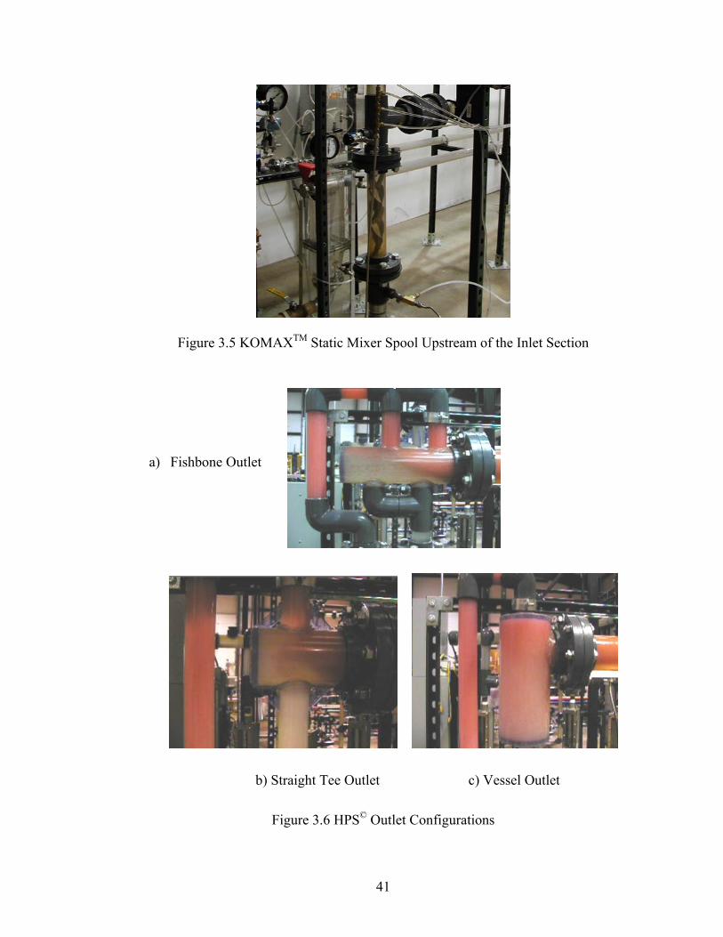


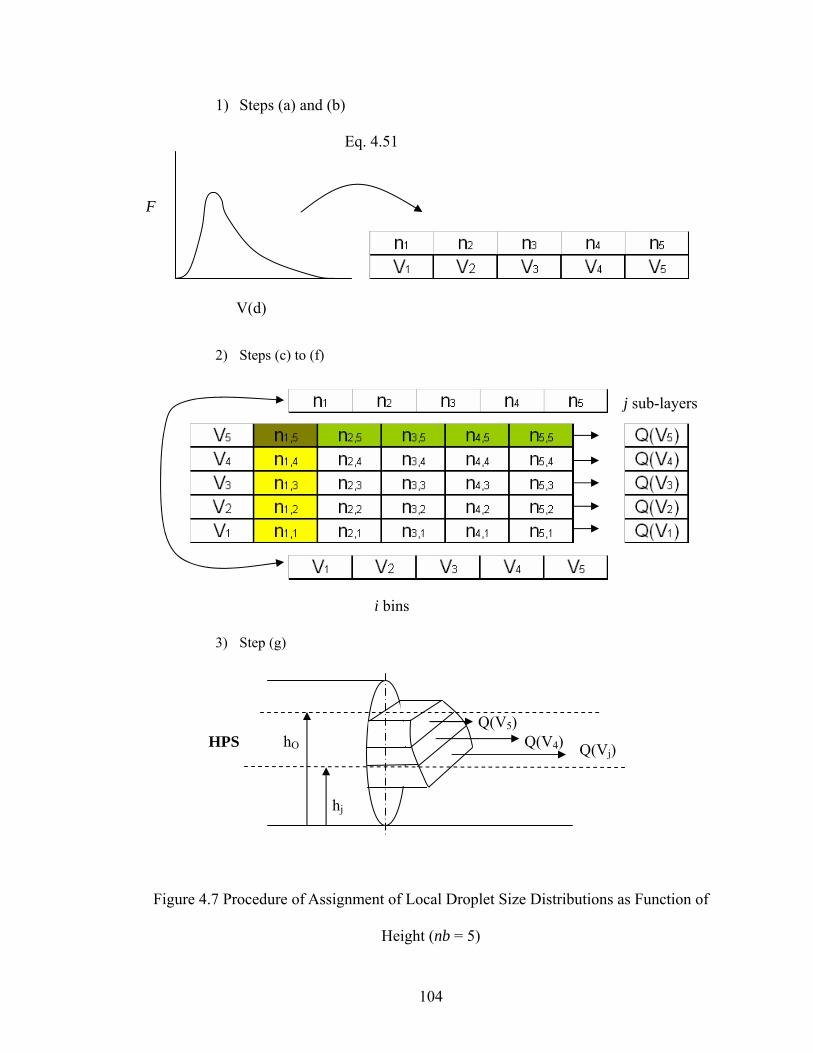


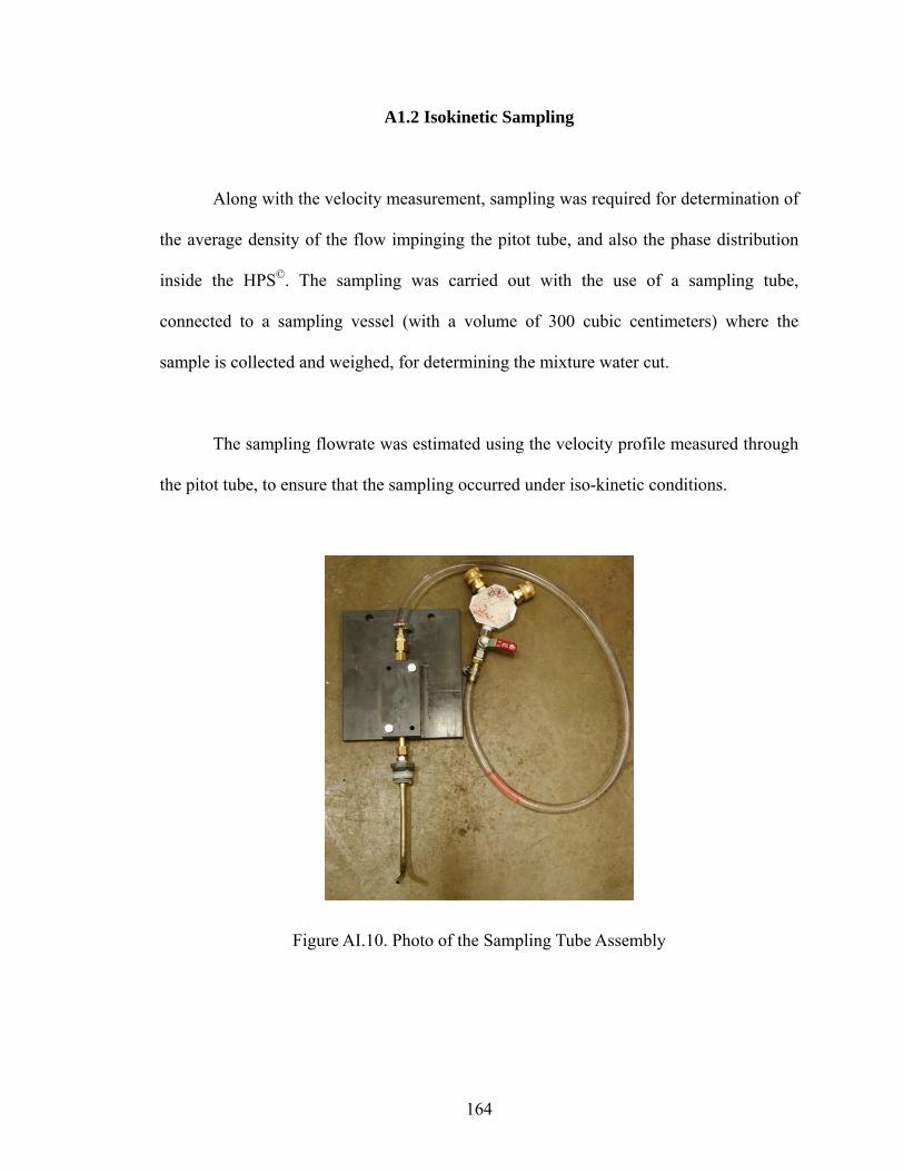


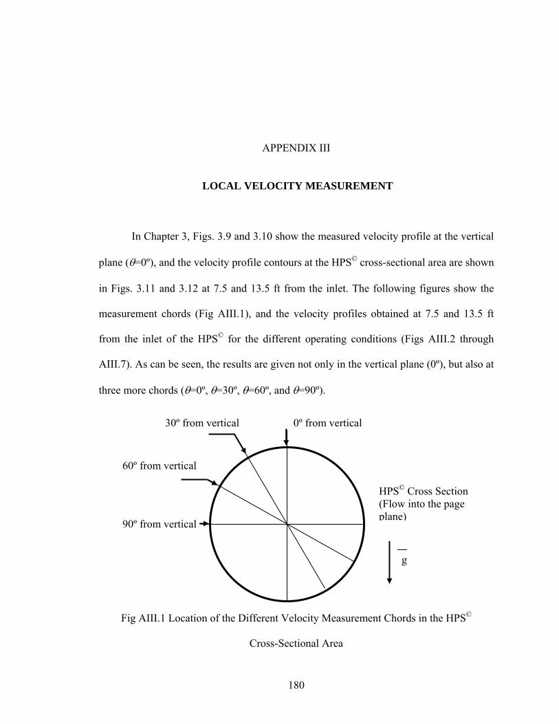


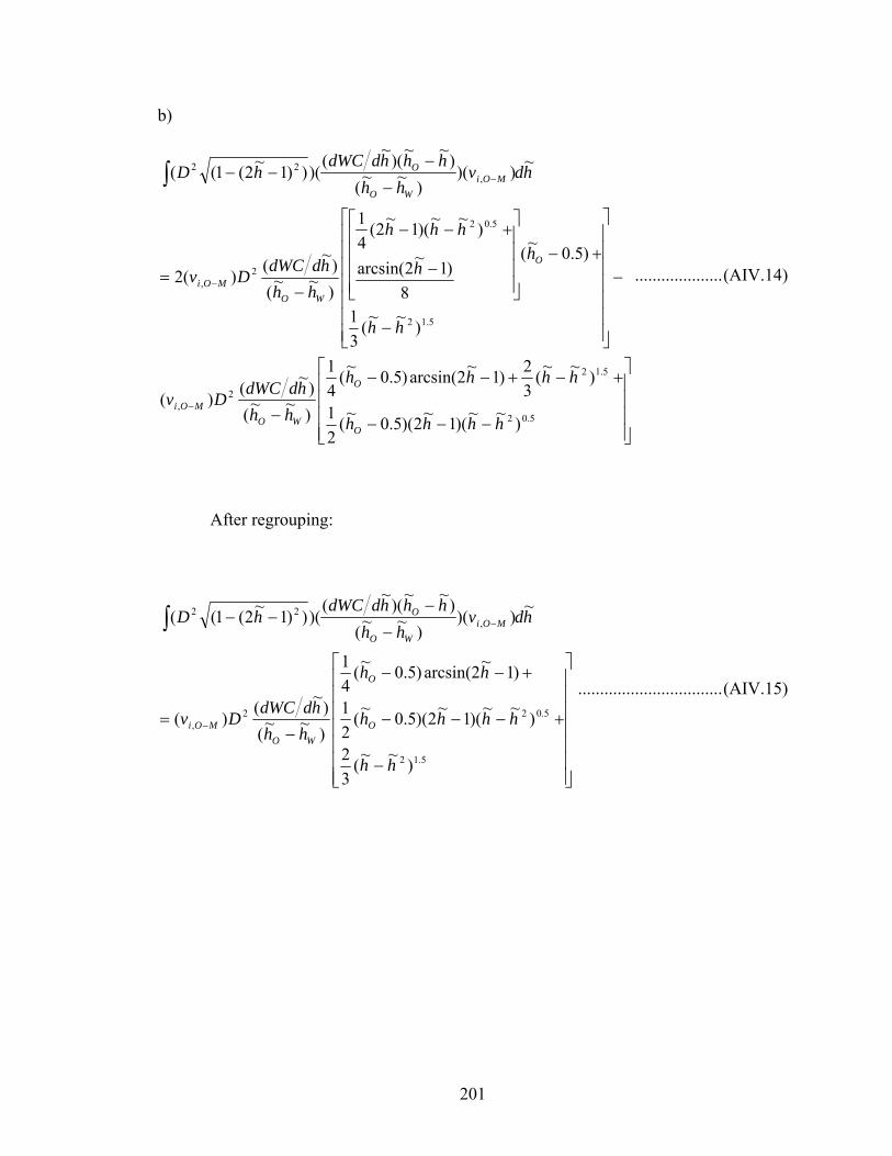


![~ a Y R p S x T T i [ g X g U n ¿ Y g Y c i s L · 2017-11-13 · c [ T r U U t ¿ c i U ] h U ¿ g ` T c i U ] Y S T j ` T Y S U r T Y t T ~ U U t L 14 e i U [ W i g U p T " François](https://static.documents.pub/doc/80x56/5f5489c62b6e9f01d05352ed/-a-y-r-p-s-x-t-t-i-g-x-g-u-n-y-g-y-c-i-s-l-2017-11-13-c-t-r-u-u-t-c.jpg)


