AD-AlSO 007 ARMY MISSILE COMMAND REDSTONE ARSENAL)AL GUIDANCE A-ETC F/6 14/2 PERFORMANCE OF LAMINAR RATE SENSORS. (U) JUL A0 A R BARBI N. J C DUNAWAY UNCLASSIFIED DRSMI/RGA-829_TR "L T TcE~E Ehh ,clllffhfhlllf
Transcript
AD-AlSO 007 ARMY MISSILE COMMAND REDSTONE ARSENAL)AL GUIDANCE A-ETC F/6 14/2PERFORMANCE OF LAMINAR RATE SENSORS. (U)JUL A0 A R BARBI N. J C DUNAWAY
UNCLASSIFIED DRSMI/RGA-829_TR "L
T TcE~E Ehh
,clllffhfhlllf
1.0
I . I ,0.25 Il I .6
O TECHNICAL REPORT RG-80-29 i
PERFORMANCE OF LAMINAR RATE SENSORS
A. R. Barbin and J. C. DunawayGuidance and Control DirectorateUS Army Missile Laboratory
July 1980
FlecImtone AF-enal, Alabaomat 36000
Approved for public release; distribution, unifiited
W1 Fo* 1"I. I JIM 79 Pffoi.C~t 01"W SOVLW 25 82 094mi e ol rdA'A
DISPOSITION INSTRUCTIONS
DESTROY THIS REPORT WHEN IT IS NO LONGER NEEDED. DO NOTRETURN IT TO THE ORIGINATOR.
DISCLAIMER
THE FINDINGS IN THIS REPORT ARE NOT TO BE CONSTRUED AS ANOFFICIAL DEPARTMENT OF THE ARMY POSITION UNLESS SO DESIG,
NATED BY OTHER AUTHORIZED DOCUMENTS.
TRADE NAMES
USE OF TRADE NAMES OR MANUFACTURERS IN THIS REPORT DOESNOT CONSTITUTE AN OFFICIAL INDORSEMENT OR APPROVAL OF
SECURITY CLASSIFICATION OF THIS PAGE ("ain Del. Fnrepd)
READ INSTRUCTIONSREPORT DOCUMENTATION PAGE BEFORE COMPLETING FORM1. REPORT NUMBER '2. GOVT ACCESSION No. 3. RECiPIENT'S CATALOG NUMBER
TR-RC-8(0-29 C)NMAA c-o,4. TITLE (and Subtitle) 5. TYPE OF REPORT & PERIOD COVERED
Perfrmane o 1,ainarRat Senors6. PERFORMING ORG. REPORT NUMBER
7. ArHOR(8~r S. CONTRACT OR GRANT NUMBER(e)
J. C. Dunawav
S. PERFORMINIG ORGANIZATION NAME AND ADDRESS 10. PROGRAM ELEMENT. PROJECT, TASKCommander, "TS Army Missile Commnd AREA & WORK UNIT NUMBERS
ATTN: TRSMI-RPTRedstone Arsenal, AL 358998
I1. FONTOLIfNG O.'Cy ANEAD~ DRESS 12. REPORT DATE_0 mmn e JI NM )r, JArmy ~1ssM il ommand July, 1980ATTN: DRSMI-RPT 13. NUMBER OF PAGESRedstone Arsenal, AL 3589q 60
14. MONITORING AGENCY NAME & ADDRESSQif different fromt Conutrolling Office) I5. SECURITY CLASS. (of tis report)
Unlassified
IS*. DECL ASSI FICATI ON.DOWN GRADINGSCHEDULE
16. DISTRIBUTION STATEMENT (of this Report)
Approved for public release; distribution unlimited.
17. DISTRIBUTION STATEMENT (of the abstract mitered In Block 20, ff different fromt Report)
IS. SUPPLEMENTARY NOTES
19. KEY WORDS (Continue on reverse side It necessary mid identify by block number)
Laminar Rate Sensor"lu id ics'Pluerics
A20. r~~c Cetmue - ,vsreu ed If ecee.y sad idenifit by block rnmber), Lainarrate sensors fabricated with present state-of-the-art etchingt qu were studied and found to have undesirable features which include:
sure., and (3) sensitivity of gain to temperature.
Null sensitivity to supply pressure was considered to be most significant.Analysis showed that the following were contributors to null bias sensitivity;(1) asymmetrv of flow separation from nozzle wall: (2) interference between 'the
JAN 147 EDITION OFI NOV S5SIS OUSOLETE UCASFE
SECUhTY CLASSIFICATION Of THIS PAGE (Whein Date Enteted)
SLQM17 Y CLASSIFICATION OF THIS PAGE(Whan~ Data Entered)
-e coitrolege, (3) wall roughness; (4) plane-to-plane alignment; and (5)
vent f low pattern asymrnetries.
%hclemos for adjusting the null bias to a zero slope region are presented.
A\ temperature compensation technique is also presented which also interacted.,t1the sensor null bias. These techniques will require individual tuning
e' ach sensor.
SECURITY CLASSIFICATION OF THIS PA6E(When Date Entered)
29. Relation of zero slope and zero offset points .. ....... 55
4
I' - .-. 62L
I N NfOD Cf I OiN
A 1. ui ia r Rite c isr (LIR'-) is a I I u id: dev ice w!.. I i1 detctts !1Ldo fle ct ioti of a thliin l am inar Ject re lat i \,, to it ; r-ot at in i; I iousin,4 as ad if fe rent i I output ic ro,,- two r'ceiVer port ;ii: , rcclit in:i' the Jet . The
F III id J c t does nor t~ dc 1 c Lt re a at iv, t o ine r L. £a I spa cec , rat hier , t hie r-c e iverport., thCiecVt- Move, due to rotat ion ot the o ; in out of a centered,zero--; ignIal 110it ion rI-lat iVe to the it . Fifntrc I depict; the operation ofthe device. F. iIp pa ren it a n plIe of d ef Io ect io n of t he 1lmina r j et , a t arotat ion rate o I iS, iven 1bv
where tf (!,note !I'' [mke of fI ;h1t of ;i fltid i'.p-11: ice from nozole l to
re-eiver, no .0 a~ (o:':'le veoetv I ad 1. is the, ;ritlcr
distance. ( iv.'n t hat tilt ouitput of tnie device is proport tona-l te i, Fqua-t ion
(1) shows that this output is directly proport ion~il o angular rate
There has been a stron ' effort over the past decade to develop thelaminar rate sensor to the stage where it could be integrated into a missilc.roll rate control system. This effort has not been a complete success.Problem areais havc been ident ifijed, howeve r, and some improvements in desigrand! perform iife '. 1) ':o evl At present , .3ome inhierent ' 1-itat ionsStill cx i.st 071 t! c of the dcv ice.
Ffi Jnrec ili luetrites sevveral designs Of rate sens~or. Three earlyG. E. designs (R( e~rence 1) Are illnstrated in Flyrs2Wi , '(ii), and
2 (i i EaIch Of Lhlec0 des; isUt i Ii ,cd a cent el duinp vent and a 2-dimeonsionalcavity in the free _jet reioin. In aidd ition, ein2 (iii) 1had Control portsand a cavity deeper than the- suppiv e:'. Ile . Des ig ,ns I and IT- were plaguedwith problems- rcusd by receive:- Iii vorfices.Y'e IT gn Iad a rat her lowmomentum recovery which waL, :itt:-i it ed to thle C:17itV d epthi. The splitter indesigns 2(1) u, and 2"(kii) Wt!Q 1la(cd approximaitely 50 noz.-Ie widthsdownstream. Tests- onl 0. sign 2 (ii i) utili in m two proportitonal amplififersreportedly indicate] a linear ran11ge of AI00 des/lsec. a thres hold of opproxi-mately 0.012 dee],,, . d i 1 La;; drift oif 0.0)2 do' over 30 minut es. In lightof later test4 %e c onne logls strnu c Com,,pany, (Ret erenc.. 2)using a more accutrate test ing setup, no c~onfidence can DeInt ced in thesenumbers.
The ~ ~ .raesno egn ii Il':strated in Figure 2 ( iv) was adapted byGE from a NASA/-angley design oif a laminar proportional amplifier (Reference3) which has a splitter distance oif 9 nozzle widths. Originally, GE soughtto improve the gain of a 3-stage laminar proportional amplifier (L.PA) gainblock. The stageable gain of the des-ign .'(iv) was approximately 10. ThisLPA performed better than any of their designs as a laminar rate sensor MLRS)and it was adopted as the standard sensor in subsequent GE LARS work (Reference4). rt should be noted that CE haid extreme difficulty staging their LPS'sinto a 3-stage gain block. Upon adding a third stage of amplification, noiselevels increased dramatically, probably because all vents were tied together,allowing a feedback path to the vent and control ports of the IRS. As
recogoizv ,]. lio laminate 15ign was also a factor in the noise levels
observed. ,I ocK,,d port o'ins (V the I.RS, with no amplification, were reportedto be
. Pa at an aspect rat io of , = 0.6
and
0.0b7 .at a 'idegr /soc
[he i, if -,ickt ! metal laminates to fabricate laminar ratesensors and 1limin.tr r.-:.,-rt mil amplif iers requires tighter tolerances thanfluidic ,,p I !c s onerati:m iIl the turbulent flow regime. Entrainment ratesof laminar iets art, cE.rtml Iv smiall .i,.d, therefore, sensitive to the exitingvelocit profile of the Jet from the supply nozzle. Small asperities on thenozzle wall ,an ,ff c't h , :it rai inment rates and the angle of the jet atthe nozzle exit. CE f'ound th,,at identical planforms etched by Bendix fromaluminum and titaniu: (dimensional repeatibilitv - 0.0025mm) showed remarkableimprovement in null h*avi,,r and .ain sensitivity ambient pressure changesover (,E etched copper lamin.,tes (dime.. nsional repeatibility - 0.025mm)(Reference 5). With this kn,.wlCdgC, CE ran a series of tests on deviceswhich had en1 ex:per i ment aIv opt i i zed in a rather clever way. Faultylaminates in a -tack were idientlfied by testing for null behavior beforeand after "fo ipl in&' of the laminate 1800 about its longitudinal axis (Refer-ence 6). Tn t -iway, t-rosS.lv fa:lt' laminates were eliminated. Tests ofsensors so constructed (with ampl if icat ion) were run with Bendix-fabricatedstainless and titanium laminates. Null shifts from 0.067 to 0.40 deg/sec Pasupply pressire, variation were. 'ncountered. It is of interest to note thatthere were measurable differOnces in those laminates held to the tightestdimensional control ra.sihie.
.'W.( "-und that tht. ra te sensors fabricated hv CE exhibited exces-sive sensitivity to Lnvironments of altitude, temperature, vibration, andacoustics (Reference *'). Also, large null shifts with supply pressure wereexperienced. Threshold, resolution, and drift did not seem to be problemareas (at least for the 25-1000 °!sec systems tested). MDAC also testedBendix titanium and stainless units. .oise in the stainless units werefound to be significantly lower than either the copper or titanium units. Anull shift of "89 0 /sec over a supply pressure range of 1744 ± 124 Pa wasmeasured.
A series of tests were performed by MDAC in an effort to optimizethe geometry of the laminar rate sensor (Reference 7). Control port width,control edge width, splitter distance, receiver width, and aspect ratiowere systematically varied to opt imize gain. Figure 3 illustrates thegeometry of the interaction region. Fable I lists the range of parameterstested by MDAC and those chosen as "optimum".
The MDAC optimization tts were conducted at ambient temperaturewith vents sonicallv isolated from the surroundings (Pvent = 210 kPa). Allof the planforms were etched by M.ODAC from 5-nil titanium, holding tolerancesto 0. 005mm.
i6
A summary of the performance of various laminar rate sensors, as
measured by MDAC, is presented in Table II. It is the opinion of this writer
that little confidence can be placed in the tests conducted by CE*, and,
thus, none are included in Table II. Also, the table does not include sensoramplifier packages. Thus, the performance figures listed pertain only tothe sensor. Staged gain, noise, etc. could be quite different than thelisted values, and would depend on the gain block design, etc. The numbersin Table II should be viewed as optimistic values since they represent thebest performance numbers out of all tests run on the designated devices.
II. PROBLEM AREAS
At this stage of its development, the laminar rate sensor hasseveral troublesome attributes. These are: (1) small signal levels; (2)noise; (3) null sensitivity to changes in supply pressure; and (4) degradationof performance with temperature change.
A. Small Signal Levels
As indicated in Table II, gains of laminar rate sensors are in the0.08 - 0.30 Pa/(deg/sec) range with exact values depending on the planformdesign and the operating conditions. Amplification on the order of - 5xi0 5
is required to increase the signal to a useful level (- 7 k Pa) for an angularrate of 1 deg/sec. Such amplification can be accomplished fluidically withoutintroduction of extraneous noise if proper attention is paid to staging andmanifolding techniques.
B. Noise
The noise levels given in Table II are, with the exception of the
stainless unit, too large for use in a 1 deg/sec system. It is believed thatthe main sources of noise in a laminar rate sensor are the wall roughnessescaused by the etching process. The Bendix-etched titanium and stainlessunits had identical planforms with, ostensibly, identical dimensional repeat-ibility ( -0.003 mm); yet, the titanium unit had approximately 3 times the noiseof the stainless unit. Figure 4 depicts the signal output of a stainlessrate sensor fabricated at MICOM when operated at two different supplypressures. The noise levels observed are of the same order as that givenin Table II for the Bendix unit. Also, the noise level (in equivalent deg/sec)is lower at the lower pressure. Roughly, the output varies directly as thesupply pressure (i.e., as the square of the velocity) while the noise (as apercent of the output signal) varies as the square root of the supply pressure.
(i.e., as the velocity).
*The reason for this lack of confidence is the accuracy of pressure measure-
ment employed by GE(- 0.27 Pa) compared to that of MDAC (- 0.0013 Pa). Thisnecessitated (noisy) fluidic amplification of the signals with no way toinfer blocked port gain of the sensor alone. GE did run some tests at NADC
in 1975 (accuracy 0.013 Pa); however, the controls on the rate tableburned out and the table had to be spun by hand with rate readings taken
from a tachometer.
7
L. . . -- -. , . 4 '**, * ,.
The size of the roughnesses on the nozzle walls is difficult todetermine. No data can be found on the average roughness height for etchedmetal laminates. However, there does exist some information on etching ofphotoceramic material,. Fluidic devices etched from photosensitive glassconsist of cavities with a floor. The depth of the cavity is determined byetching times. Van Tillburg (Reference 8) reports average roughness heightsof "0.0004mm on the cavity floors, but the walls were found to have roughnessesaveraging -O.O025mm. Since both were exposed to the same etchant, the rela-tively rough walls must he the result of the technique (artwork, exposure,etc.) used to transfer the planform pattern to the glass. The same techniqueis utilized to prepare metal laminates for etching and it is reasonable tosuppose that metal laminates would have walls no smoother than the glasswalls. Thus, in the absence of better information, we assume that theaverage roughness height on the nozzle is at least on the order of 0.0025mm.
C. Null Shift
Perhaps the most serious deficiency of a laminar rate sensorintended for use as a low angular rate sensing device is its null shift withsupply pressure changes. Figure 5 illustrates this behavior. As indicatedin the expanded curve (about the operating point), the slope of this curveis rather steep. The output signal corresponding to a rotation of 1 deg/secis shown for comparison.
The exact shape of the null curve is a function of the fabricationand assembly of the device. To illustrate, Figure 6 shows the change in thenull curve accompanying a change in position of the individual laminates inthe stack (three 0.12 7mm stainless laminates). For identification, the lami-nates are numbered from the top cover plate in the first case (1-2-3), curveA in Figure 6. Also shown is the effect of rotating ("flipping") the centerlaminate about its longitudinal axis (contrast curves C and D). The impli-cation of this behavior is that, with the present state of the art in fabri-cating etched metal laminates, the possibility of mass-producing sensors withpredictable and repeatable null behavior is remote.
If it is supposed that the null shift is due entirely to misalign-ment of the downstream splitter, the angle of the jet with the centering ofthe device should not change and one would expect the null shift to be propor-tional to the dynamic pressure of the jet, i.e., to the supply pressure.However, this behavior is not observed. Evidently, the angle of the jet doeschange with supply pressure. Two causes could effect such a change. First,the separation points of the jet on either side of the nozzle could be slightlydifferent due to slight radius differences and/or roughnesses just upstreamof these points. Second, slight differences in nozzle wall roughness couldaffect the entrainment rates on either side of the jet and cause it to bend.In all likelihood, both effects are present to some extent. Each of theseeffects would be functions of the nozzle velocity.
Separation of the jet from the nozzle walls can be analyzed if thevelocity profile at the nozzle exit can be estimated. Toward this end, con-sider the nozzle illustrated in Figure 7.
It is assumed that the boundary layer on the wall has zero thicknessat the inlet to the converging section and, following Shearer and Smith
"' II I
(Reference 9), the velocity profile within the boundary layer is taken to besinusoidal. Thus
V
V sin() (2)
where Y denotes distance perpendicular to the wall, 6 is the nominal boundarylaver thicIanes:, and V is the potential core velocity. For the convergingsect ion, fro-T .'ont inuitv
VVp x sa (3)
- sin ,/?2
,S S
Vsa denotes the average velocity at the nozzle exit. For the nozzle underconsideration (HDL design 3.1.1-005Ci
W/B = 4.63S
a= 570
Equation (3) thus becomes
VsaV -
p 4.63-0.48 X/B (4)s
For the sinusoidal velocity profile, equation (2), it is not difficult toshow that
0 = 0.13666 (momentum thickness) (5)
6* = 0.36345 (displacement thickness) (6)
and
T = 1.5708 uV /6 (shear stress) (7)p
The von karman momentum integral equation may be written as
dV
T20+ V2 dO +*)V p (8)p dxp dx
Using ,!quations (4) - (7), equation (8) may be recast in the non-dimensionalform
9
- - . -
. 2 37 )6~ 1 ____9 (9).. .. .. :' rx .,2 =
(4.63-0.48/B) j2 Rb
whore N V S1 SP .vnolds number based on nozzle width some manipula-
atio:'. ;1V' is a first-order, linear, non-homogeneous differentialeq!Jation which -in be s:,,Ivvd with the aid of an integrating factor. ItsSolution is
N ,¢, = i-0.104 9 . 2 1 o... ... ... d. (.
( o-o. I
A numerical irterat ion of cquat ion (I) :ro:- 0 to 3.88 yields avalue of (N, ) at the inlet to the nez: le t 1rea t of
RI
or
. *i ?548s .5 Nb-(12)
rqLiation (12) gives thc displacement thickness at the entry tothe throat of the' no'zle. %';chIichting's (Reference 10) solution for aparallel plat channel (entry region) should hold in the throat section.Thus,
5* t = kQ"(.vetx )/V (k = 1.72) (13't sa
where Ove is equivalent length defined as that approach distance required toyield the displacement thickness given by equatIon (12) at xt = 0. Thus
2.548 k \v;veNRb V k 1 2
sa 4
,q in
I0
or
've= 2.9q5 (14)
The displacement thickness at the exit of the nozzle is thus
-k .(2.195 R + x
sa
or
53.57 3.25k .. (15)
s N Rb NRb
for the nozzle under consideration.
If it is assumed that the boundary layers on the side walls andend plates are equally thick, we can get an expression for the dischargecoefficient of the nozzle. -,he volume rate Q can be expressed as
Q= v B H (16)sa
s
or, alternately, as
Q = V - 2 6)(H- 2 (17)
where Vs denotes the potential core velocity at the nozzle exit and H is theheight o4 the nozzle (i.e., the distance between the end planes). From(16 and (17),
Vsp * Vsa (18)
B s ( aBwhere a = H/Bs . Expansion of equation (18), yields
sp I + 2 + . ( I+2 6Esa s s
I + 2(1 -)--- . (1)S
11
f.I
If we neglect term-, of order ,reater thaii (. /B) we can get the approximateoxpression
V 2(1 + ) V 6.50(1 + c) (2)
sV BSd .Rb
using equat ion (I). The disC'hargte coeffici(It is simply the ratio of the
average velocitv at tx it tO 0 potent iZ1 core velocitv there. Thus,
(N) (21)
sp 1 + -- -
"'Rb
ithe point of separit ion of t In 5Io.,, from the nozzle side wall canbe calculated (to within 1") with Strat'ord's technique (reference 11);(see Figure 8 for no:,encl ature) . At the point of separation
CO, -(X X 0. Ol C'. (22)
where
V
Cp = - 2 (preqsure coefficient) (23)sp
x
x(d = X - 1_ 2 (24)XF m 0.45v Esp
x designates the development distance (along the wall) of the boundary laverand x m represents the minimur pressure point (point A in Figure 8); Xm is5.179 B for nozzle x' is the length of a flat plate required to develop ablasius-profile at point A vtth the same momentum thickness, Pp., as the actualboundary layer. The integral in equation (24) was evaluated using Walz'approximation (Reference 10).
The pressure coefficient of the flow downstream of point A, up to
separation, can he found from the potential solution over the rear of acylinder. Thus,
V = V cos:p sp
and-): (25)
C = - coF. { = sin' .
12
thus,
dcP/d x 2 sin f Cos I- sit, I cos 1 (26)= dx R
Stratford's equation (22) may now be written as
sin- cos(sn'j = 0.0104 (27)R R R
The term (x)/R in equation (27) is simplified as follows: Fromequations (5) and (6),
E = 0.376 * E (28)
Thus, from (24),
' Vsp -
m 3.185v
or
x-x V 5* -= m + spR R 3.185vR (29)
Equations (15) and (19) can be utilized to express equation (29) as
X-X BR R B [1 6.50(1+a)]R- R + 3. 317 R : 1 + --N R (30)
Substitution of equation (30) into (27) yields ( after a bit of manipulation)
JY + 3.317 1 + 6.50(1+c,) sin Y sin 2Y - 0.10198 = 0R G-N RbS s(31)
x -Xwhere Y s m the angle of separation.s R
Equation (31) indicates that the separation point depends on theReynolds number and thus on the supply pressure. If both walls were ofexactly the same radius, the separation points would be identical and the jetwould remain centered. Consider, however, the situation depicted in Figure 9,where there exists a difference in radii on either side, and a small errorA in the position of the centers of these radii. In this case, the jet will
13
* I
make an angle S with the ccnterlin, tf (Reference 12)
= A+ R sin :s,, - R sin"'arCLal Is + R(1 - R- (132
lB + C -s's)+R cos 'Ys, 32
and this angle will depnd on NRb"
The effect of the jet arngle S will show up as an output or null
shift. It is presumed t!t saturation of the LRS occurs when the jet is
deflected to th.' Toint where its ( intercepts the center of one receiver port
(see Figure IP) . This "saturatjiuoT angle" is given by
I' : arctan( (33)
R
for the micom. LRS (with T = 1.2'), y = 2.684 deg.. The output associated
with deflection S will be
APo K Ps - (34)
where K is the "gain" of the device. Figure 11 shows an input-output curve
for the LRS used herein. For this device
K - 0.77
Figure 12 is a plot of null output vs. supply pressure for the
LRS with the gain curve shown in Figure 11. The LRS was operated with both
control ports vented to ambient. The sensor was fabricated from five,
equation (34), the jet deflection angles were calculated at several points.These angles are plotted in Figure 13. Also shown is a plot of jet deflection
angles calculated from equations (31) and (32) with an assumed radius of0.127mm on one wall and 0.114mm on the other. As indicated in the Figure,
the jet deflection angles calculated from separation considerations vary
only slightly with supply pressure (the analysis does not hold for Ps < 150 Pa
since it predicts boundary layer thicknesses > Bs/2 there). The jet deflec-
tion angle derived from the null output data, however, varies linearly with
supply pressure, except near Ps = 0 and beyond Ps = 200 Pa. Thus, although
some "steering" of the jet could be ascribed to the separation process at the
nozzle exit, this cannot account for the observed behavior.
The region downstream of the nozzle exit and up to the control
edge is illustrated in Figure 14, which also contains a caiculated velocity
profile at Ps=249 Pa. At this point the boundary layer thickness is - 0.22mm,
which is large compared to the nozzle half-width of 0. 2 54mm. The control
edge setback for this LRS is quite small, 0.032mm from the jet centerline.
At the conditions illustrated, separation is predicted at an angle Y. = 2.85
deg. If the edge of the jet were to be at this angle, the Figure indicates
that it would intercept the control edge (point P). It should be noted that
14
'a
- . . . . . - . , .
Manion and Drzewiecki's analysis predicts a clearance between the controledge and the entrainment streamline of -O.O05mm for these conditions. Itis clear that significant interference effects could exist in this amplifierbecause of the small control edge setback. Before ascribing the entire nullbehavior to this interference, however, we should recall that the nullbehavior of the optimum MDAC device was essentially no different from thepresent unit, even though it had a relatively large setback which allows forangles of spread (11.7 0 ) approximately 5 times those of the present device(-2.4o). Calculations have been made for the MDAC unit operating at Ps
= 1.87 k Pa, a = 0.50, which indicate a jet spread angle of -1.5 deg.
it is clear from the foregoing, that the null behavior (i.e.,shift) with operating pressure changes cannot be explained by changes inseparation on the nozzle walls, nor is it related to jet control edgeinterference effects. The null shifts observed translate into jet deflectionangles -0.2 deg, approximately 10% of the angle required to saturate thedevice but -325 times the deflection encountered by the jet in a rotation of1 deg/sec, i.e. -0.00062 deg. (from equation (1)).
At a rotation rate of I deg/sec, the jet deflection of 0.00062 degtranslates into a lateral movement of 0.0001mm at the receiver ports. Thisis a distance some 27 times smaller than the dimensional repeatibility possiblein etching metal laminates. When viewed in this way, it is indeed surprisingthat the LRS works as well as it does. These small distances suggest anotherpossible explanation of the cause of the null shifts. When viewed from thereceiver port, the nozzle appears as indicated in Figure 15. The walls arenot perfectly smooth. As the supply pressure increases, the velocity profileflattens, the boundary layers on the top and bottom end plates become thinner,and those "layers" of fluid close to the plates exert an increasing influenceon the total dynamic pressure. The same behavior translates to the splitter-receiver region where the momentum intercepted by the receivers is increasinglyinfluenced (as supply pressure increases) by the fluid adjacent to the plates.As these regions near the plates (nozzle and splitter) are "uncovered" theycan cause slight shifts in the momentum intercepted by the receivers. If theroughness elements are on the order of 0.0003mm, it is conceivable that theycould effect strong enough changes to be measured.
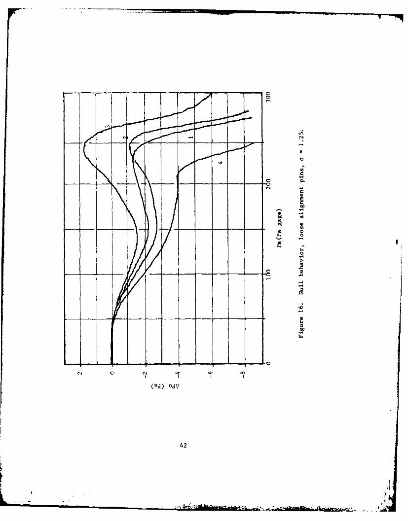
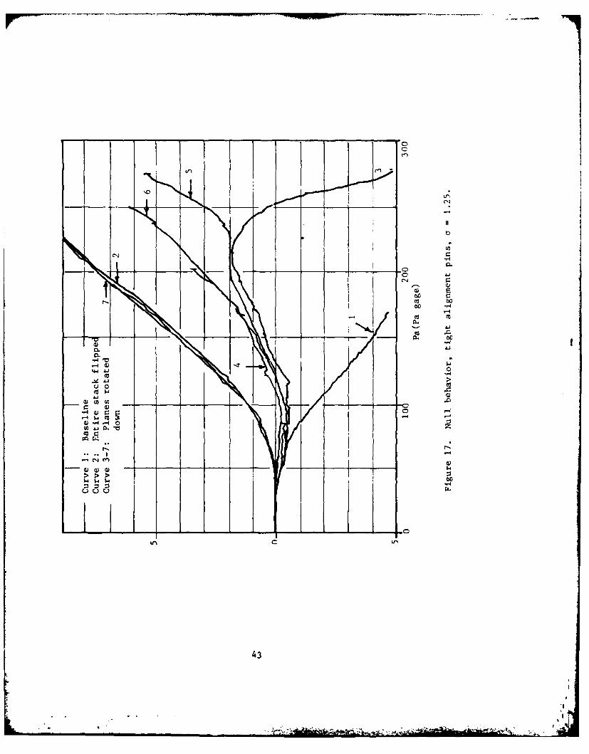
Even if the walls were perfectly smooth, the metal planes could bemisaligned, as indicated in Figure 15 (ii), and the same effect would beobserved. There will always be some misalignment due simply to the dimen-sional repeatibility of siting the alignment pin holes in the laminates.Figure 16 illustrates how the null shift curve may be changed by shiftingthe planes in a stack with loose fitting pins. Each successive curve wasrun after loosening the clamping screws, tapping the cover plates, and thenretightening the screws. We have already seen in Figure 6, that shifting therelative position of laminates in the stack, and "flipping" them can drasti-cally alter the null curve. Figure 17 illustrates the same effect for astack of five laminates with tight fitting pins. Seven curves are shown inFigure 17; #1 is a reference configuration. Curve #2 is the null behaviorof the stack upon "flipping", i.e., rotating, 1800 about the longitudinalaxis, of the entire stack. One would expect a curve identical to curve 01with a polarity change; however, this does not occur. The only differencebetween curves I and 2, other than polarity, is the vent flow which is allowed
15
_ -. '', . .. .. o.;)
to pass through only one of Lhe end plates. Curve 3 through 7 were succesivelyderived by rolling the stack down one plane each time; curves 2 and 7 areidentical, as expected.
At this point, it might be conjectured that the null shift behaviorcould be considerably improved if a LRS could be constructed from a singlelaminate, and thereby eliminate the problem of plane-to-plane alignment. Tocheck this out, a null curve was run on a corning 1x CD, 0.25mm proportionalamplifier. This amplifier was not intended to be a laminar proportionalamplifier, nor a rate sensor. However, by operating in the laminar regime,we were able to get a rate signal (albeit small) and a null curve, which ispresented in Figure 18. Even here, a null drift with pressure is observed.
D. TEMPERATURE SENSITIVITY
As part of their evaluation program of fluidic laminar rate sensorsfor the Naval Air Systems Command, 4DAC (Reference 2) ran tests on laminarrate sensors (supplied by GE) at -46C, ambient, 38C, and 74C. Gain and noisewere the two parameters most affected by temperature variations. A loss ofgain was experienced with elevated temperatures, while gain increaseswere encountered at low temperature. Noise levels increased with bothextremes with the colder temperature producing the largest increase.
On the basis of their tests, MDAC found that gains could increaseas much as 1.5 times from ambient down to -46C (though all their tests didnot indicate this) and it could decrease by a factor of 3.5 from ambient to74C. This behavior is expected since the dynamic pressure of the jetdecreases with temperature.
The increase in noise associated with increasing and decreasingthe temperature is difficult to explain. It is believed to be related to thetechnique of temperature conditioning. Conditioning air was circulated aroundthe sensors during testing by a blower mounted in a remote temperaturechamber. The sensors were shielded from direct wind currents but they werevented to ambient. In the presence of air flow, noise can easily feed throughto the vents of the sensor and show up in the output. Figure 19 illustratesthe effect of turning on a room-type air conditioner approximately 12 feetfrom a test setup. Two effects are noted: (1) a long term drift which isdue to a cooling (temperature) effect, and, (2) an increase in noise due toturbulent air flow over the test area from the circulating blower of the A/Cunit. The increase in noise observed by MDAC in their temperature tests isbelieved to be of the same source.
The long term drift illustrated in Figure 19 is a result of the changeof resistance with temperature of the dropping resistor upstream of the sensor.With a change of temperature, this resistance changes, the suppiy pLe"SULtchanges, and the null drifts (see paragraph 3 above). This proved to besomewhat troublesome in the course of one series of tests which were initiatedby energizing a normally-closed solenoid in the supply line. With the droppingresistor downstream of the solenoid and being influenced by the heating effectof the solenoid, the supply pressure drifted at the rate of -0.025 Pa/secwhereas, with the resistor upstream of the solenoid, this driftrate was-0.013 Pa/sec. Using the slope of the null curve at the operating point,
16
the predicted drift with time agrees very well with the observed null drifts,(Figure 20).
Gain change with temperature occurs primarily because of a changein the dynamic pressure .v2 , of the jet. As temperature increases, viscos-ity increases and causes (for the same pressure drop) a decrease in velocity.To maintain the dynamic pressure constant as temperature increases, thepressure could be increased. Isueh (Reference 13) has shown that if the supplypressure is made to vary as Ta , where a is the temperature exponent ofviscosity (0.71 -t < 0.5), the dynamic pressure of the jet will remainessentially constant with temperature. It was also shown that the requiredpressure variation could be implemented by placing an orifice upstream of thenozzle with an area I one-tenth of the nozzle area. The onlv experimpntperformed to date to verify the theory was performed by Hsueh on a nozzle.The pressure on the nozzle does indeed increase with a temperature increase,though it approaches the theoretical value for area ratios of 1/100 or less.The effect on gain has not been experimentally verified.
The nozzles utilized in laminar rate sensors have areas rangingfrom 0.129mm 2 , (0.508mm, 1 . :' - to 0.323mm 2 (0.508mm, o = 1.25). Compen-sating orifices for these .1o 7 * will range from 0.127 - 0.203mm diameter
at 1/10 area ratios. Thbs s , afford partial temperature compensation.In practice, however, < r ±que could not be used because of the null
shift problem. To illus: ca"- for proper temperature compensation betweenambient and 74C, the prt..,_ i-.t the nozzle would have to increase by
P74/ .1 7273 ++ 74 1I.21
/Pamb (273 + 74 1.22 ( = 0.5)
an increase of 22%. Pressure changes of this magnitude would be manifestedas rather significant, and unacceptable, null shifts.
E. PRESSURE SENSITIVITf
In view of the sensitivity of null to supply pressure, it is impor-tant to maintain accurate regulation of the pressure at the nozzle of a lami-nar rate sensor. The setup used in the tests on the MICOM LRS isillustrated in Figure 21.
To get an idea of the pressure regulation achievable, a series oftests was run, some of the results of which are presented in Figure 22 whichillustrates the supply pressure vs. time upon manual opening of valve A.Several pressure histories are illustrated. The initial pressure overshootand decay are apparently caused by the capacitance of the lines preceedingthe solenoid; one does not observe this behavior when cycling the solenoidvalve with the regulators loaded (Figure 23). As indicated in Figure 22,the spread in the various curves is -10 Pa. Undoubtely, some of the variationis due to normal room temperature fluctuations between tests, though it ishard to quantify the effect. Ignoring the temperature effect, we can conserv-atively estimate the set point repeatability of the pressure regulationscheme of Figure 21 as -10 Pa at a nominal operating point of 249 Pa, i.e.,as ± 2% of set point pressure. There is no reason to suppose that a special
17
- - . -- - -*. ~ ., .
purpose regulator with the smae repeatability cannot be developed. The curveshown in ',,re 23 ill,:, rate a long term drift in supply pressure (O.0125Pa/sec) whiii i- belikved to be a temperature effect on the supply resistor.Also shown is the rapid response of supply pressure to opening and closingthe solenoid valve upstream of the .RS. As indicated above, the transientassociated with pressurization of the lines upstream of the regulators(Figure 22) is not present.
Refere:ce to Figure 5 illustrates the effect of the supply pressureset-point or, t., oressure r gulation requirements. For the case illustratedin Figuro 5, .tn of the device at a supply pressure of 143 Pa (i.e.,at the fl, spot (,f' tLe null shift curv, ") would require a pressure regulationof ± 5 Pa (, 3.5') to maintain null uncertainty of 0.50 deg/sec. If the samedevice were operated at 162 Pa, however, pressure would have to be maintainedto - 0.33 Pa (_ 0.2') to ensure the s.tme null uncertainty. In comparing thenull sensitiviti,. of different ser-,rs, care must be taken that each isoperated at romp u-ahl] points on the iiull curve. MAC (Reference 7) made theclaim that t ir "oPti711, unit" achieved an improvement of 2 orders of magni-tude in null sh!"t Over th L! ndix-f-hricated stainless unit. Closer inspec-tion reveals, ho!ecr, hat MDAC was comparing its unit's operation at a flatspot with Bendix unit's 0perat .L), at a point removed from a flat spot, andthat, in fact, Lte imnprovcment was indeed modest (see below and Table III).
-:11 scn-it vit: t- supply pressure changes, as conventionallyquoted, can he misJeading. A more .mriningfui specification of null behavioris the unit's sensitivitv to percentage regulation about the operating point.Table III lists the zsen;itivities )f several sensors in deg/sec, equivalentsignal, per 27 of qet--poi7rt rressure (the 2% figure is believed to bepresently achievable). A- inhicated in the table, the stainless units arecapable of holdi-r nul! to -,,;ithin 1.ii sec (equivalen-t signal) if operatedat a flat spot on Lh,, nail shift curve provied tne pressure is maintainedwithin 2% of the set point. It does not appear possible to hold the nullbelow 2/see variation if the units are net operated at a flat spot.
la!)le IIT .Ioes not include the null offsets and null behavior ofsome of the early GE units since their outputs were extremely noisy. Interms of equivalent rate si nals, null offsets can be large but they are notconsidered to he a problem :4ince tha'. can be compensated by biasing in theamplification chain Jasu-u:ea;:: ot the sensor, also, some biasing can beaccomplished in the sen.,r itseif (Isve Section III below).
III. NULL BIASING T;F 1711i:IOU'FS
The null behavilor of laminar rate sensors can be influenced to someextent by controlling the pressure in the control ports or by adjusting thenozzle angle (with respect to the , of the unit). Several techniques havebeen used, including:
(1) Control ports open to ambient(2) Each control port blocked(3) Control ports connected(4) Each control port vented through adjustable resistors(5) Nozzle block cantilevered and adjustable
(6) Control ports biased from supply with adjustable resitors.(7) Sensor cantilevered about splitter-receiver and adjustable with
adjustable nozzle walls.
In their optimization studies, MAC (Reference 7) ran null shiftcurves on each of 24 units tested with techniques (1), (2), and (3) above.In some units, there appears to be little difference between the three config-urations, while in others, drastic changes in null behavior occur. No generalconclusions can be drawn about the relative merits of the three on the basisof these tests. None of the three provides the opportunity of adjustmentwhich is considered desireable in view of the normal unit-to-unit differencesencountered.
CE utilized technique (4) to control bias. On the basis of theirexperience with this approach, it cannot be recommended as practical. Theamount of flow entrained by the sides of the laminar jet in contact with thecontrol port is extremely small and exerts a proportionally small aspiratingeffect. Apparently, the control port pressure is extremely sensitive to theresistance and it is hard to set the desired bias. There is another disadvan-tage to this approach; any noise delivered to the vent feeds through to thecontrol ports and is amplified thereby. This is believed to be the cause ofthe noise problems experienced by GE in their attempts to amplify the outputof their sensors. The GE AW-12 amplifiers used downstream of the sensor arenotoriously noisy; their venting into the common manifold could have been thereason that GE noted increases in the noise/signal ratio with the addition ofeach stage of amplification.
A laminar rate sensor was constructed at MICOM which had an adjusta-ble cantilevered nozzle section. By moving the nozzle transverse to thecenterline of the sensor, the shape of the null curve was considerably influ-enced. It was found that the "flat spot" on the null curve could be moved,as indicated in the sketch of Figure 24, but that in other respects the nullshift with pressure was essentially unchanged.
Garrett has developed a rate sensor package for MICOM which utilizesthe principle of nozzle angle adjustment via cantilevering of the nozzle-control port-vent region about the splitter area which is accomplished withsmall set screws and is a bit easier than the caming arrangement used innozzle-block adjustments. Also included in the Garrett design is an adjustmentwhich deflects the nozzle wall.
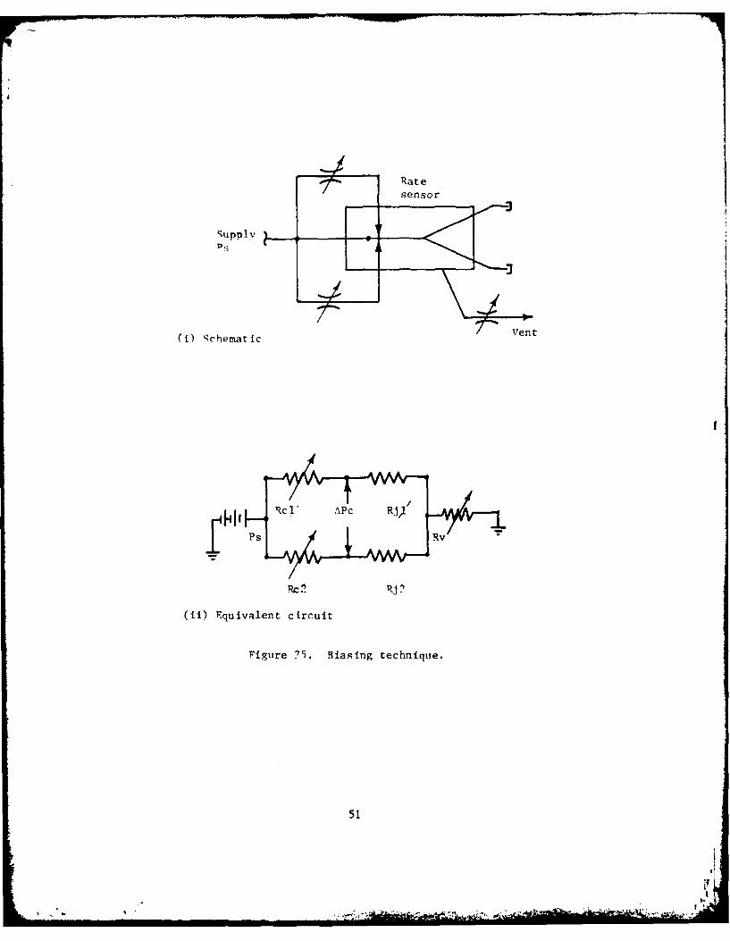
All of the tests on the MICOM sensors in this report used individualbiasing of the control ports with adjustable orifices fed from the supplypressure, as indicated in the sketch of Figure 25(i). Also, the vent wascollected and exhaustpd to ambient through an adjustable orifice. It seemedadvisable not to use linear resistors as biasing elements since their resist-ances change with temperature; a null shift with temperature would be undesir-able. In general, null offset can be adjusted, at any supply pressure, toa desired value by individually adjusting the bias controls, or by changingthe vent resistance.
The equivalent circuit of the biasing scheme used is indicated inFigure 25 (i). It is easily shown that the pressure difference across the
19
* ~ ~~ . .' ., ..-.. , . ...-.
control port is given byv
_ -Rc 1 (35)
KRA k" Rc( +c Rv(Rcl)
where
Rc Rd c I Rc " 4 Qj~ RJ 2 (36)
and
Rel , Re? 2 re s istanccs of coint ml biasing orificesRj I , Ri 2 1jet-cont roI cd, o rte istanct-Rv =vent resbi-taiice
Manion and Drzewiecki (Reference 12) have show-i that the jet-control edgeresistance is prclport iOILa'[ to the supply nozzle resistance, which is roughlyproportional te FPjTE. The other resistances are orifice types and it can beshown that each is also proportitonal to JS. Thuls,
Rcl, Rc2, Rjl.. Rj_' P~~Ps
Thus, from (35)
APc aw Ps (37)
The control port pressure difference .. Pc exerts a transverse forceon the jet exit ing from the io.:zle at ain anI . The effect is to reduce
* (or increase) this angle and therb\v to reduce (or increase) the output.*Consider the control volume intlicated in Figure 26. The net force in the
Y-direction is APcA, where A is the control port area. Using the momentumequat ion,
,IFy V -l t vin) (38)
Thus, -APcA = Vs sin V - v sin (39)
where $1 des ignates the aug c the jet leav'ing the control volume. Sincem =pA sV a
As in .1 -~ -
A V2
or, for small angles, s
A~cA 2(40)
As Vsa
- -
From equation (37),
APc - Ps Vsa
thus, equation (40) may be rewritten as,
S k1 (41)
The output of the sensor will be proportional to ,I and to the dynamic pres-sure of the jet.
.Ps = k, CR Ps (B - kI) (42)
Where CR is a "recovery" coefficient of the jet. CR is expected to increasewith Reynolds no. (i.e., Ps) since the boundary laver thickness (at nozzleexit) decreases. Assuming
CR - Ps
n
where n(C-) is unknown. Thus
APo = k3 Ps n+1 [(Ps) - k1 ] (43)
where B has been expressed as a function of Ps, f(Ps) (see Figure 13).
The rate of change of APo with Ps is given as
(APo) = (n + I)k pn(f - k) + k psn+df3Ps 3 3 dps
= (n+1)APo + k Psn+l df (44)Ps 3 dps
" PoFrom equation (44) it is noted that a flat spot (0-Po = 0) and a zero null
3Psoffset (AP = 0) can occur at the same point only when dB/dPs = 0. For theunit illustrated in Figure 13, this point occurs near 225 Pa; at lower pres-sures df/dB J 0 and equation (44) indicates that we should not expect both aflat spot and zero null offset at pressures below 225 Pa. Figure 27 and 28illustrate the effect (for a different unit than that of Figure 13). Thenull curves in Figure 27 were generated by holding resistances Rcl, Rc2constant while varying Rv while those of Figure 28 were generated by holdingRv constant while varying RcI and Rc2 . The same set of curves result witheither technique. The minimum of each curve moves toward Ps = 0 as the pointof zero null offset is decreased, whereas the maximum points increase. Asindicated, the device can be operated at a flat spot over a wide range ofsupply pressures, but there is only one supply pressure at which both nulloffset and slope are zero (275 Pa for the unit shown). For the planform
21
4•* A
used in this study there exists significant interference effects between thejet and the control edge at this pressure (see Figure 14).
Figure 13 indicates that at Ps < 200 Pa, B is roughly proportionalto Ps.
B k4 Ps (75 Pa < Ps < 200 Pa)
Thus, we can write equation (43) as
Po = k5 's n + 2 - k6 Ps n + l (45)
From equation (45)
= (n + 2)k 5 n+l - (n + )kPsn (46)Ps 56
If Ps2 denotes the zero null offset pressure,
n+2 n+lk Ps2 - k Ps 2 = 05 2 6 2
or
k6 = k5 PsI (47)
Designating the point of zero slope as Psl,equation (46) yields
n+ln
(n + 2)k5 PsI - (n + l)k6 Ps 1 = 0 (48)
Using equation (47), equation (48) may be manipulated to yield
Ps 2 n+ 2
- = (49)Ps 1 n+ 1
Equation '49) indicates that the ratio of P should be a fixed value (see
Figure 29). Inspection of the null curves of Figures 27 and 28 show thatthis is, indeed, the case and
Ps 2Ps 2 1.54 (50)
for all curves having a zero null offset. From this it is inferred that
m = 0.818 (51)
22
I'
It should be noted here that the use of linear resistors to bais
the sensor could result in an improvement in the sensitivitv of null output
to sipply pressur.. Thus, if tht. re iistanc e s Rcl, Re 2 , Kv wert- in:.deptndent
of Ps, then, from equation (35)
.'-PC = ko(Ps) (52)
and equation (3) woild become
'P = K 31 s fl+l() - kPF] (53)
At low pressures, f = k, Ps and equat ion (53) indicates that 'Po Woild stillbe a function of Ps. The slope is (upon some manipulation)
Equation (54) admits the possibility of coincident zero null and zero slopepoints. It should also he remembered that linear resistors would he tempera-
ture sensitive and would cause the null to be temperature dependent.
IV. SLUDIARY AND CONSLITSIONS
Laminar rate sensors fabricated with present state-of-the-art
techniques have several undesireable features including: (1) small signal
output, (2) sensitivity of null to variations in supply pressure, and (3)
sensitivity of gain to temperature. Enough evidence is now on hand to indicatethat significant improvement in these areas will not result from further
attempts to optimize via simple geometric changes in the planform. Nor is it
likely that novel biasing techniques will be discovered to ameliorate the
difficulties.
Presently achievable blocked-port gains of laminar rate sensors
fall in the range of 0.08 - 0.30 Pa/(deg/sec); staged gains can be as low
as 1/2 of blocked port gains. Fluid amplification (with all the attendantdifficulties of staging, manifolding, etc.) on the order of 5x10 5 is required
to increase the signal to a useful level.
Null sensitivitv to supply pressure remains the most trc:.' :esome
aspect of the laminar rate sensor. The effect cannot be attributed solely to
separation from the nozzle walls nor to interference between the jet and the
ment in the null behavior is highly unlikely with the present method of
fabrication from stacks of etched metal laminates.
The sensitivity of a laminar rate sensor decreases with temperature.
Compensation for this effect by maintaining the jet dynamic pressure constant
requires an increasing nozzle supply pressure. It appears that this can be
accomplished (at least partially). The procedure, however, would result
in significant nullshift (with the units presently available) and thus it
23
. ....- . .. ,- .6 .. i r . ,
cannot be considered as a viable solution. At present, ther exists no tempera-ture compensation scheme which does not also affect null.
The performance of a laminar rate sensor in a I deg/sec system islikely to be marginal for the following reasons:
(1) The transverse movement of the jet due to a 1 deg/sec rotation is onthe order of - 0.075 x i0-3mm. A surface finish with roughness elementsless than this would be in the superfinish catagory. With the etchedlaminates used at present surface roughnesses of - 2.5 x 10⁻³mm are likely.
(2) Noise levels of 0.3 - 0.6 deg/sec equivalent signal.
(3) Null sensitivity to pressure requires tight pressure regulation ofsupply pressure. For 27, regulation of supply pressure, null can vary
2.5 deg/sec unless care is taken to operate at a zero slope point. Nullvariations at these flat spots is - 0.2 deg/sec for ± 2% supply pressure
regulation.
(4) If the units are operated at a supply pressure where null offset is notzero, null will be temperature sensitive.
It has been found that a simple biasing scheme using adjustableorifices can be used to operate a LRS at a zero slope point over a range ofsupply pressures. Adjustable orifices (rather than linear resistors) arerecommended in order not to create a temperature-dependent biasing scheme.There does exist one supply pressure at which both null and its slope arezero (for the MICOM sensor) and, for reasons (3) and (4) above, biasing andsupply pressure should be adjusted to insure operation at this point. Withthe present fabrication techniques, this is expected to require individualattention to each unit built.
The integration of a LRS into a system will require attention to
isolation of the vent of the device from ambient (preferably via sonicorifices). In addition, care should be taken to isolate the LRS vent fromother vents in the system (e. g. downstream amplifiers) to minimize noise inthe LRS output.
24
i'; ' | "
Table 1. MAC OrTi'MZATION TESTS (Reference 7)
I TEM RA N T- OPTIMIM UNIT
Control port width 1-8 B 6 BS S
Control edge width 1.5 - o B 3.5 B
Splitter Distance 8-2n B 16 BS S
Receiver width 1-2 B 1.5 B
Aspect ratio n.25-1.25 0.5
25
0. CL 0 -
I'- -
to r'
W Hh
0 0D ZF W~ *
1~ 0-
H H H CD
I-'IV
-t 00 - - 1
En-m
V 14 Ln 0
00 0
mJ 00 1 " M
L.) 41 IDtn
262
4P -,
Z- F-u
=c~ -4<~
Cc 'T' -.
a) C
- C!
Cr c-C :: c Q) QC
- CC C) - -i E- -
toC
on.
F- 2-
Nozzle L
Figuire 1. Lamrinar rate sensor.
28
I-
~.J ~
-,.~ > f
I-I-
'-40.
-~C.,
I fE
z
-4
4.-1~.
o
U..
If 4.-
aJ
1.-
-40
0U
-4'-4'-4
0.
rz~ ~4O
CJCiU
~a~G)C.,>
a) -4-4 0N 1.4W2
4J4.J0
z 00
29
*0
A. . *44.- -. .., 1.'
BS = Nozzle width
T oto pr it
C B'F Control edge width
B~1,[ X~j = Splitter distance
B, Receiver width
2, ~enpar tor
Figure 3. Geometry of interaction region of a laminarrate sensor.
Figure 21. Bench test setup - pressure regulation.
47
I!
30
10 Pa
20 ___ ____
10 secTime
Figure 22. Repeatability of set point supply pressure.
48
f4 0
00
b)C0
C..
tc
-4 0,-
0-0
494
c)N
41
1% 1f
0
Rat esensor
Sulpply
(1) Schematic Vent
VIC Yd APc Rj / 4-
(ii) Equivalent circuit
Figure ?5. Biasing technique.
51
PcA
Figure 26. Control volume definition sketch.
52
L .' . '• t,
r C~
w cto Q'
Q ! aC r
C'44
4
o'>- 0a
0L
U'-' -
N
' '4;
-r4
-VA.
Cu
-'--v-- '4 / ~I 0 0'
t*4 IN-I
t-i-----h--- . 0~C
I -4
-4
54
Ps2 P.2 1.54IPS I PS I"°
APOI PS
Figure 29. Relation of zero slope and zero offset points.
55
NOMENCLATURE
Symbols
B Control port width
B Receiver width0
B Nozzle widthS
B Control edge widthr
CD Nozzle discharge coefficient
C Pressure coefficient
p
f( ) Unspecified function
H Nozzle height
k, k -k Constants (defined in text, as used).17
K Gain
Ze Equivalent flat plate boundary layer lengthto produce a proper displacement thickness atnozzle erit
LR Distance from nozzle to receiver
1m Mass flow rate
n Exponent
NRb Reynold's number V saB V
Pc Control port pressure
Po Output port pressure
Ps Supply pressure
Q Volume flow rate
R Radius
Rc Resistance of control bias orifice
56
--* , * - '.,- m-L . -_ -,, I_ *
Rj Jet control edge resistance
Rv Vent resistance
tF Time of flight of a particle from nozzle toreceiver
T Temperature
V Velocity
V Potential core velocityP
V Average nozzle exit velocitysa
V Potential core velocity at nozzle Oexitsp
W Width at nozzle entry
X Boundary layer length
y Equivalent flat plate boundary layer lengthto produce a proper momentum thickness atnozzle exit
Xm Location of minimum pressure point
x s Location of separation point
xsp Nozzle-to-splitter length
y Distance perpendicular to wall
a, , Y9 T Angles (defined in text, as used)
6 Nominal boundary layer thickness
6 Displacement boundary layer thickness
A( ) Difference
C Centerline distance along nozzle
r Distance from center of receiver port to centerof splitter
Viscosity
V Kinematic viscosity, p/p
57
T ~-
Angular velocity
P Density
CY ~ Nozzle aspect ratio, H/B
Shear stress
EJ Momentum boundary layer thickness
X EX/B
Subscripts
( ) Nozzle exitE
( )~ Nozzle throat
t'
58
REFERENCES
1. "Feasibility Investigation of a Laminar Rate Sensor (LARS) Phase IReport", Reader, et al, GE document no. 69SD698, 20 June 1969, NavalAir Systems Command.
2. "Evaluation Program Fluidic Laminar Rate Sensor", Westerman and Wright,MDAC report L0252, 8 March 1974, Naval Air Systesm Command.
3. "A Fluidic Roll Rate Control for High Acceleration Guided Missiles",Onufreiczuk, GE document no. 73SD2041, Interim Report, March 1973, MICOM.
4. "Feasibility Investigation of a LARS, Phase IV Final Report," Young,GE document no. 73SD2147, August 1973, Naval Air Systems Command.
5. "Final Report, Fluidic Roll Rate Control System for High AccelerationTerminal Homing Missiles." Young, GE document no. 745D2053, April 1974,US Army Missile Command.
6. "Feasibility Investigation of a LARS, Phase IV Final Report", OnufreiczukYoung, and Gresham, GE document no. 75SDR2173, April 1975, Naval AirSystems Command.
7. "Fluidic Laminar Angular Rate Sensor Development Program, Final Report",G. W. Roe, MDAC report L0317, 17 April 1975, Naval Air Development Center.
8. "Production of Fluid Amplifiers by Optical Fabrication Techniques",R. W. Van Tillburg, Proceedings of the Fluid Amplification Symposium,October 1962, V-1, p. 143-156.
9. "Some Analytical and Experimental Studies of Laminar Proportional Ampli-
fiers", Shearer and Smith, HDL-CR 76-213-1, April 1976, (Penn State Univ.).
10. Boundary Layer Theory, Schlighting, Mc-Graw Hill, 1968, p. 177.
11. "Approximate Methods for Predicting Separation Properties of LaminarBoundary Layers", Curle and Skan, Aero-Quarterly, Vol. VIII, p. 257,August, 1957.
12. "Analytic Design of Laminar Proportional Amplifiers", Manion and Drzewiecki,Fluidic State-of-the Art Symposium, Vol. I, 30 September - 3 October,1974, p. 201.
13. "Temperature Effects on Fluidic Laminar Rate Sensor", P. ,sueh, AppendixC of GE document no. 69SD698, 20 June 1969, Air Force Contract no.F33615-68-C-1700.
59
-All . .
DISTRIBUTION
No. of Copies
Defense Technical Information CenterCameron StationAlexandria, Virginia 22314 2
A. R. BarbinM. E. DepartmentAuburn UniversityAuburn, Alabama 36840 2
V. H. BaumgarthARRADCOMATTN: DRDAR-SCF-CCDover, New Jersey 07801 1
John BurmeisterNaval Weapons CenterATTN: CODE 3636China Lake, California 93555 1
James CarrHQ, DOE/GERMANTOWNMail Stop F309Washington, DC 20545 1
Peter F. DixonUS Army ARRADCOMATTN: DRDAR-LCU-MDover, New Jersey 07801 1
T. M. DrzewieckiHDL, ATTN: DELHD-RT-CD2800 Powder Mill RoadAdelphi, Maryland 20783 1
J. C. DunawayUS Army Missile CommandATTN: DRSMI-RGC, Bldg 5400Redstone Arsenal, Alabama 35898 1
Keith L. EnglanderNaval Ordnance StationCODE 5123CIndian Head, Maryland 20640 1
A. J. GarrettPacific Missile Test CenterCODE 3122Point Mugu, California 93042 1
60
DISTRIBUTION (Continued)
No. of Copies
Michael GoesUS Army ARRADCOMATTN: DRDAR-LCN-CDover, New Jersey 07801
John M. GotoHDL, ATTN: DELHD-RT-CD2800 Powder Mill RoadAdelphi, Maryland 20783
Richard N. GottronHDL, ATTN: DELHD-RT-CD2800 Powder Mill RoadAdelphi, Maryland 20783
Richard HellbaumNASA, Langley CenterMS 494Hampton, Virginia 23665
Dean HouckNaval Air Systems CommandATTN: AIR 5162C8Washington, DC 20361
Tor JansenNaval Air Development CenterCODE 60134Warminster, Pennsylvania 18974
James W. JoyceHarry Diamond LaboratoriesATTN: DELHD-RT-CD2800 Powder Mill RoadAdelphi, Maryland 20783
David KeyserNaval Air Development CenterCODE 60134Warminster, Pennsylvania 18974
Daniel C. KinneyHQ AFOSI/IVTSRBolling AFB, DC 20332
Keith KlaberDepartment of Transportation400 7th Street, SWWashington, DC 20590
R. L. McGiboneyNaval Air Development CenterCODE 60134Warminster, Pennsylvania 189714 1
R. Michael PhillippiHDL, ATTN: DELHD-RT-CD2800 Powder Mill RoadAdelphi, Maryland 20783 1
James L. PowellDOE - FE 44Washington, DC 20545 1
Albertus E. SchmidlinUS Army ARRADCOMATTN: DRDAR-LCN-C, Bldg 65Dover, New Jersey 07801 1
Gene SpratkeUS Army TARADCOMATTN: DRSTA-RCAFWarren, Michigan 48090 1
Bill WaldonNaval Weapons CenterChina Lake, California 93555 1
James A. BurkeHQ, Dept of~ the ArmyATTN: DAMA-WSAWashington, DC 20310 1
John E. BurnsNaval Air Systems CommnandCODE AIR-5 162CIWashington, DC 20361 1
George W. FosdickApplied Technology LaboratoryATTN: DAVOL-ATL-ASAFt Eustis, Virginia 23604 1
Al FranzUS Army ARRADCOMATTN: DRDAR-LCN-FDover, New Jersey 07801 1
DISTRIBUTION (Continued)
No. of Copies
CommanderUS Army Training and Doctrine CommandFt Monroe, Virginia 23341 1
CommanderUS Army Combined Arms Combat Development ActivityFt Leavenworth, Kansas 66027 1
CommanderUS Army Armor CenterDirectorate for Armor AviationATTN: ATSB-AADO-MS, LTC Don SmartFT Knox, Kentucky 40121 1
HeadquartersDepartment of the ArmyATTN: DAMA-WSM, MAJ BelchWashington, DC 20310 1
CommanderUS Naval Weapons CenterATTN: Mr. J. A. KnechtChina Lake, California 93555 1
DRCPM-HF 1-HFE, Mr. J. Service I
DRSMI-X 1DRSMI-R, Dr. McCorkle 1
-R, Dr. Rhoades 1-R, Mr. Black 1-RG 1-RGC 20-RGT 1-REO 1-REI 1-RE 1-RR, Dr. Hartman 1-RR, Dr. Guenther 1-RR, Dr. Gamble 1-RN, Mr. E. Dobbins I-RPR 5-RPT Reference Copy 1-RPT Record Copy 1
DRSMI-LP, Mr. Voight 1
63
k _ ' :_ . . .... .... ... '- ... .a
Distribution (Concluded)
No. of Copies
Douglas GarnerNASA, Langley CenterMS 494Hampton, Virginia 23665
George C. !opcsakOUSDRE( ET)Pentagon, n.", _)L.03Washington, DC 20301
James PapadopoulosSMD Advanced Techrv logy CenterP. 0. Center 1500Huntsville, Alabama 35807
Ken ReaderASED - CODE 1605Naval Ship R&D CenterBethesda, Maryland 20084
Harry M. SnowballAF Flight Dynamics LaboratoryATTN: AFFDL/FGLWright-Patterson AFB, Ohio 45433
Robert N. WareUS Army MERADGOMATTN: DRDME-EMAFt Belvoir, Virginia 22060