3.1 Introduction ........................................................................................................................... 3-33.2 Study Area Boundaries ......................................................................................................... 3-33.3 Compilation of Shoreline Development Data ........................................................................ 3-33.4 Existing Shoreline Conditions ............................................................................................... 3-3
3.4.1 Developed Shoreline by Land Use or Allocation ................................................... 3-33.4.2 Undeveloped Shoreline by Land Use or Allocation ............................................... 3-53.4.3 Developed Shoreline by Ownership Category ...................................................... 3-53.4.4 Developed Shoreline by Reservoir ....................................................................... 3-63.4.5 Reservoir Subdivisions ......................................................................................... 3-63.4.6 Residential Shoreline Alterations .......................................................................... 3-63.4.7 Average Depth of Reservoir Shoreland ................................................................ 3-8
3.5 Shoreline Vegetation ........................................................................................................... 3-113.5.1 Introduction ......................................................................................................... 3-113.5.2 Shoreline Vegetation Types ................................................................................ 3-113.5.3 Forest Area and Tract Size ................................................................................. 3-14
3.7 Endangered and Threatened Species ................................................................................ 3-183.8 Soils ............................................................................................................................ 3-18
3.8.1 Introduction ......................................................................................................... 3-183.8.2 Climate ................................................................................................................ 3-183.8.3 Soils of the Blue Ridge ........................................................................................ 3-223.8.4 Soils of the Valley and Ridge .............................................................................. 3-223.8.5 Soils of the Cumberland Plateau ........................................................................ 3-223.8.6 Soils of the Highland Rim.................................................................................... 3-223.8.7 Soils of the Nashville Basin ................................................................................. 3-243.8.8 Soils of the Coastal Plain .................................................................................... 3-243.8.9 Shoreland Soil Erosion ....................................................................................... 3-243.8.10 Shoreline Bank Stability ...................................................................................... 3-25
3.9 Wetlands ............................................................................................................................ 3-263.9.1 Introduction ......................................................................................................... 3-263.9.2 Wetlands Mapping and Interpretation ................................................................. 3-273.9.3 Wetlands Analysis Zones and Acreage Calculations .......................................... 3-273.9.4 Wetlands Functions and Values .......................................................................... 3-273.9.5 Wetlands Trends ................................................................................................. 3-28
3.10 Floodplains/Flood Control ................................................................................................... 3-293.11 Aquatic Habitat .................................................................................................................... 3-30
3.11.1 Introduction ......................................................................................................... 3-303.11.2 Benthic Macroinvertebrates ................................................................................ 3-303.11.3 Fish Communities ............................................................................................... 3-313.11.4 SAHI and Existing Conditions ............................................................................. 3-32
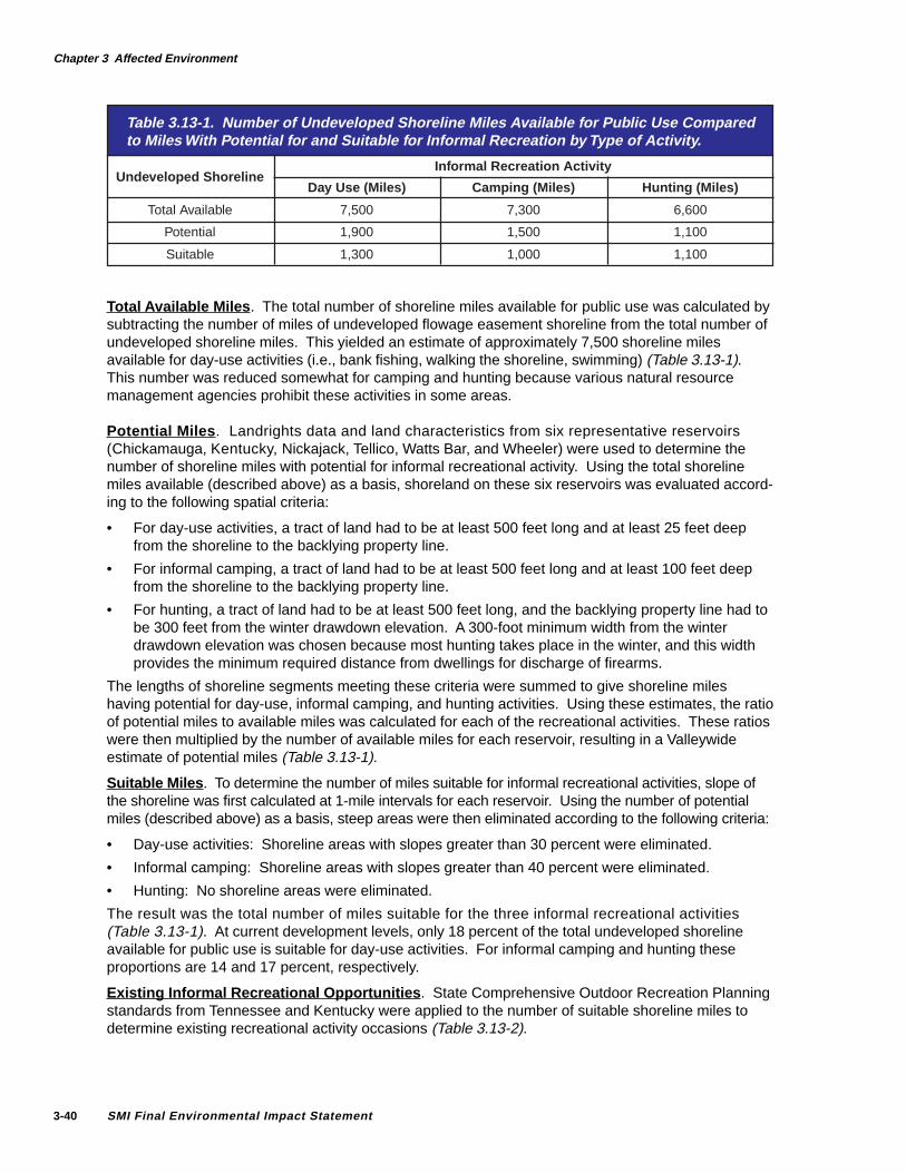
3.13 Recreational Use of Shoreline ............................................................................................ 3-373.13.1 Introduction ......................................................................................................... 3-37
Click on page number to go to that page. Use Find from the Tools menu to search for text.
3.13.2 Total Visitation ..................................................................................................... 3-373.13.3 Recreation Activities Occurring Along the Shoreline ........................................... 3-373.13.4 Informal Recreation ............................................................................................. 3-39
3.14 Aesthetic Resources ........................................................................................................... 3-413.14.1 Introduction ......................................................................................................... 3-413.14.2 Findings of the Gallup Poll, TVA Land Management and Use Study,
January 1993 ...................................................................................................... 3-413.14.3 SMI Public Scoping ............................................................................................. 3-413.14.4 Results of the TVA Questionnaire, Viewing Tennessee
Valley Shoreline .................................................................................................. 3-413.14.5 Existing Conditions ............................................................................................. 3-42
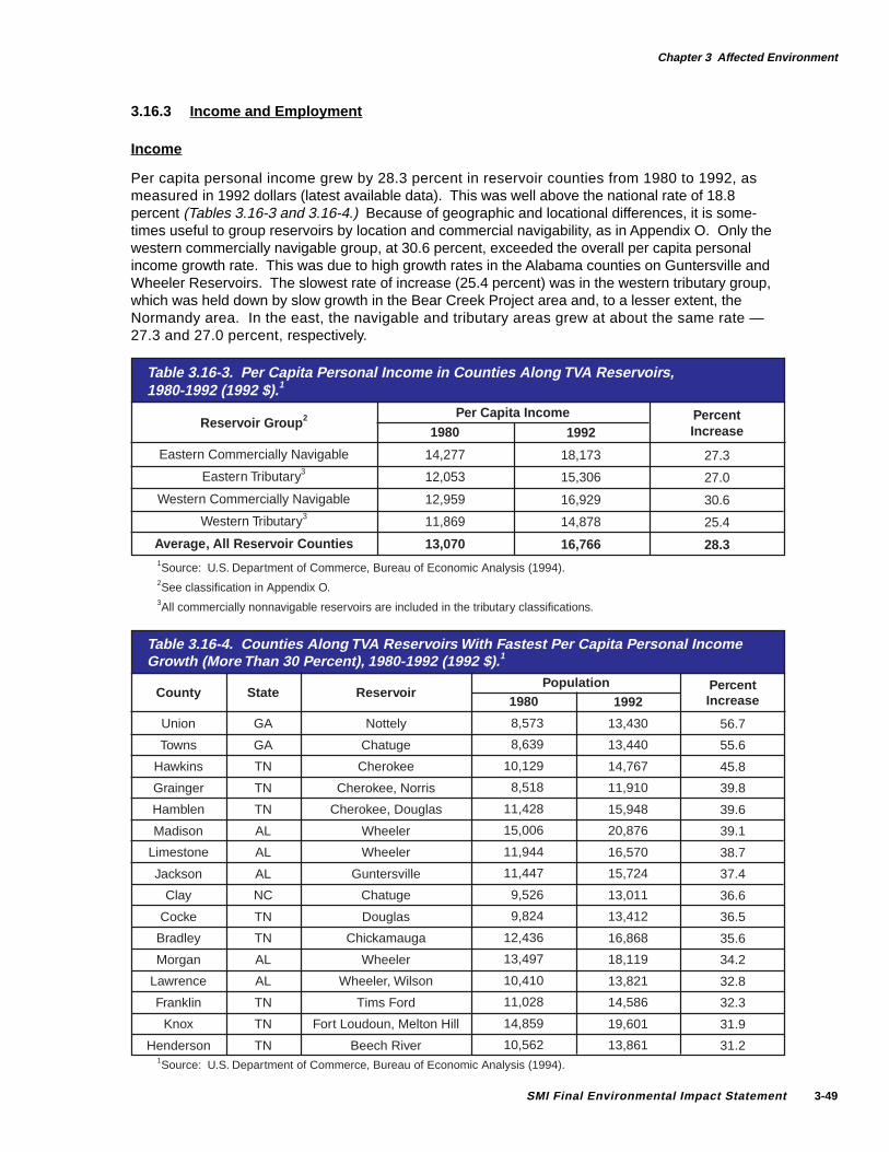
3.16 Socioeconomics .................................................................................................................. 3-443.16.1 Introduction ......................................................................................................... 3-443.16.2 Population ........................................................................................................... 3-443.16.3 Income and Employment .................................................................................... 3-493.16.4 Property Values ................................................................................................... 3-503.16.5 Tourism ............................................................................................................... 3-513.16.6 Environmental Justice ......................................................................................... 3-52
3.17 Navigation ........................................................................................................................... 3-523.17.1 Introduction ......................................................................................................... 3-523.17.2 Commercial Navigation ....................................................................................... 3-523.17.3 Navigation Aids (Including Safety Harbors and Landings) .................................. 3-533.17.4 Recreational Navigation ...................................................................................... 3-533.17.5 Recreational Navigation Aids .............................................................................. 3-53
Reminders:
In each numbered section of the chapter, the first mention of an alternative will be in bold print.
Alternative A - Limited TVA Role Along Open Shoreline and Additional AreasAlternative B1 - Existing Guidelines Along Open Shoreline and Additional Areas (No Change/No
Action)Alternative B2 - Existing Guidelines Along Open Shoreline OnlyAlternative C1 - Managed Development Along Open Shoreline and Additional AreasAlternative C2 - Managed Development Along Open Shoreline OnlyAlternative D - Minimum Disturbance Along Open Shoreline OnlyBlended Alternative - Maintain and Gain Public Shoreline
Please see the Glossary in Chapter 5 for the meaning of unfamiliar words.
Ownership Categories on 10,995 Miles of TVA Reservoir Shoreline
• Flowage easement shoreland
• TVA-owned residential access shoreland
• TVA-owned-and-jointly-managed shoreland
• TVA-owned-and-managed shoreland
Chapter 3 Affected Environment
SMI Final Environmental Impact Statement 3-3
AFFECTED ENVIRONMENT
CHAPTER 3
3.1 Introduction
Chapter 3 provides baseline information for understanding environmental and socioeconomic impactsassociated with SMI alternatives analyzed in Chapter 4, Environmental Consequences. More specifi-cally, this chapter describes the setting and existing conditions of natural, social, and economicresources that would be affected by the SMI alternatives. Resource issues to be discussed in detail are:
• Shoreline Vegetation• Wildlife• Endangered and Threatened Species• Soils• Wetlands• Floodplains/Flood Control• Aquatic Habitat• Water Quality• Recreational Use of Shoreline• Aesthetic Resources• Cultural Resources• Socioeconomics• Navigation
Chapter 3 also includes a description of the study area boundaries, an explanation on compilation ofshoreline mileage data, and a discussion of existing shoreline conditions.
3.2 Study Area Boundaries
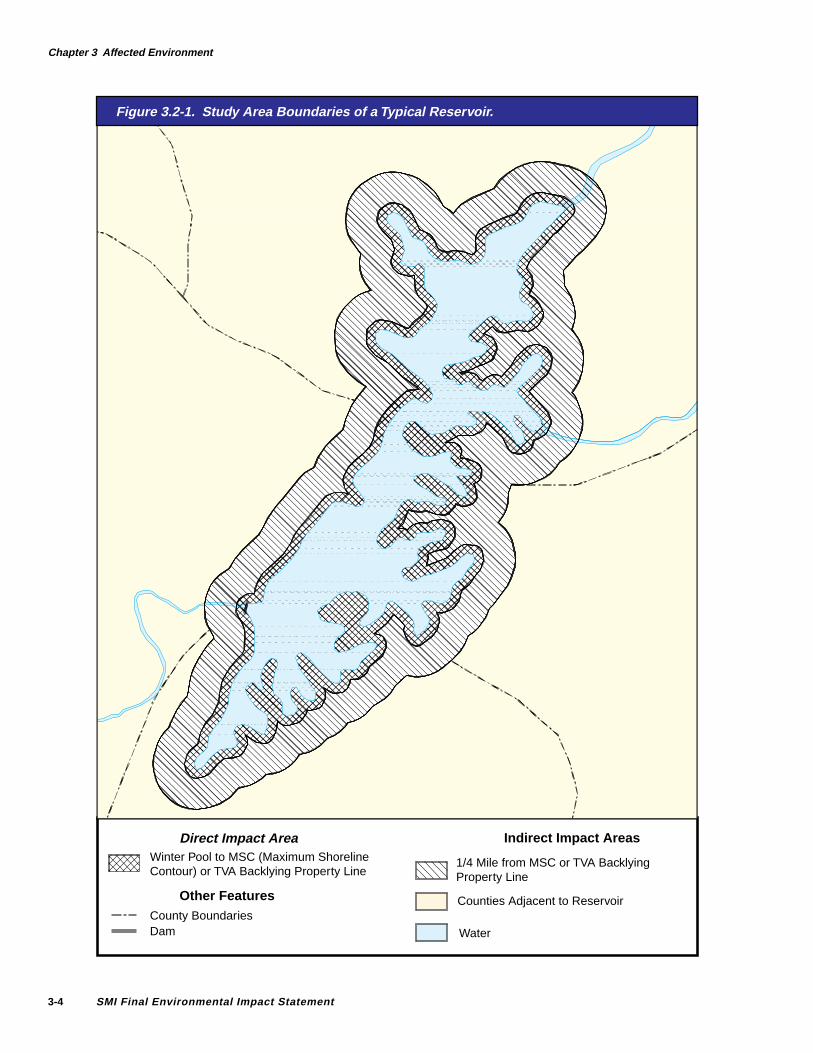
The study area boundaries used in Chapter 4, Environmental Consequences, are shown inFigure 3.2-1. The boundary for direct effects is the area between winter pool elevation and themaximum shoreline contour or TVA backlying property line (whichever is farther from the shoreline).
Indirect effects are measured on (1) adjacent private lands one-fourth mile from the maximum shorelinecontour or TVA backlying property line (approximately equal to the average depth of a subdivision),(2) the remainder of the reservoir area (both above and below the lake surface), and (3) countiesimmediately adjacent to the reservoirs. However, the study area boundaries of some resources willvary, especially the boundaries associated with consideration of cumulative impacts.
3.3 Compilation of Shoreline Development Data
In 1994 TVA’s Land Management Offices conducted boat surveys of TVA reservoir shorelines anddelineated developed and undeveloped shoreline segments on topographic maps. Segments wereidentified as developed if shoreline structures such as docks and retaining walls were present. Ifvegetation disturbance also occurred, then the total extent of the disturbed area was marked asdeveloped. These field data maps were digitized using TVA’s GIS, and miles of developed, undevel-oped, and total shoreline were computed for each reservoir.
3.4 Existing Shoreline Conditions
3.4.1 Developed Shoreline by Land Use or Allocation
As the population and economy of the Tennessee Valley have grown, so have the pressures for theuse and development of land surrounding TVA reservoirs. As of 1994, development from all uses had
Chapter 3 Affected Environment
SMI Final Environmental Impact Statement3-4
Figure 3.2-1. Study Area Boundaries of a Typical Reservoir.
Direct Impact AreaWinter Pool to MSC (Maximum ShorelineContour) or TVA Backlying Property Line
Other FeaturesCounty BoundariesDam
Indirect Impact Areas
1/4 Mile from MSC or TVA BacklyingProperty Line
Counties Adjacent to Reservoir
Water
Chapter 3 Affected Environment
SMI Final Environmental Impact Statement 3-5
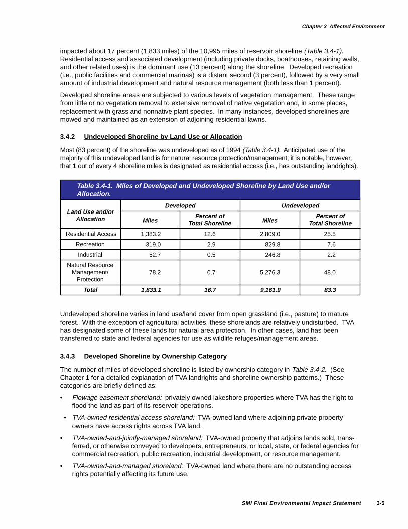
impacted about 17 percent (1,833 miles) of the 10,995 miles of reservoir shoreline (Table 3.4-1).Residential access and associated development (including private docks, boathouses, retaining walls,and other related uses) is the dominant use (13 percent) along the shoreline. Developed recreation(i.e., public facilities and commercial marinas) is a distant second (3 percent), followed by a very smallamount of industrial development and natural resource management (both less than 1 percent).
Developed shoreline areas are subjected to various levels of vegetation management. These rangefrom little or no vegetation removal to extensive removal of native vegetation and, in some places,replacement with grass and nonnative plant species. In many instances, developed shorelines aremowed and maintained as an extension of adjoining residential lawns.
3.4.2 Undeveloped Shoreline by Land Use or Allocation
Most (83 percent) of the shoreline was undeveloped as of 1994 (Table 3.4-1). Anticipated use of themajority of this undeveloped land is for natural resource protection/management; it is notable, however,that 1 out of every 4 shoreline miles is designated as residential access (i.e., has outstanding landrights).
Table 3.4-1. Miles of Developed and Undeveloped Shoreline by Land Use and/orAllocation.
Developed Undeveloped
Percent ofTotal Shoreline
12.6
2.9
0.5
0.7
16.7
Miles
2,809.0
829.8
246.8
5,276.3
9,161.9
Percent ofTotal Shoreline
25.5
7.6
2.2
48.0
83.3
Miles
1,383.2
319.0
52.7
78.2
1,833.1
Land Use and/orAllocation
Residential Access
Recreation
Industrial
Natural ResourceManagement/
Protection
Total
Undeveloped shoreline varies in land use/land cover from open grassland (i.e., pasture) to matureforest. With the exception of agricultural activities, these shorelands are relatively undisturbed. TVAhas designated some of these lands for natural area protection. In other cases, land has beentransferred to state and federal agencies for use as wildlife refuges/management areas.
3.4.3 Developed Shoreline by Ownership Category
The number of miles of developed shoreline is listed by ownership category in Table 3.4-2. (SeeChapter 1 for a detailed explanation of TVA landrights and shoreline ownership patterns.) Thesecategories are briefly defined as:
• Flowage easement shoreland: privately owned lakeshore properties where TVA has the right toflood the land as part of its reservoir operations.
• TVA-owned residential access shoreland: TVA-owned land where adjoining private propertyowners have access rights across TVA land.
• TVA-owned-and-jointly-managed shoreland: TVA-owned property that adjoins lands sold, trans-ferred, or otherwise conveyed to developers, entrepreneurs, or local, state, or federal agencies forcommercial recreation, public recreation, industrial development, or resource management.
• TVA-owned-and-managed shoreland: TVA-owned land where there are no outstanding accessrights potentially affecting its future use.
Chapter 3 Affected Environment
SMI Final Environmental Impact Statement3-6
% of TotalShoreline Developed
5.9
6.7
3.1
1.0
16.7
TotalMiles
2,345.2
1,847.0
4,043.2
2,759.6
10,995.0
DevelopedMiles
645.0
738.2
343.3
106.6
1,833.1
Table 3.4-2. Miles of Developed and Total Shoreline by Ownership Category.
% of OwnershipCategory Developed
27.5
40.0
8.5
3.9
Landrights Category
Flowage EasementShoreland
TVA-OwnedResidential Access
Shoreland
TVA-Owned-and-Jointly-Managed
Shoreland
TVA-Owned-and-Managed Shoreland
Total (or Percent)
The proportion of total shoreline currently developed under flowage easement is only slightly lessthan that of residential access shoreland (6 percent and 7 percent, respectively). However, becausethere are fewer miles of residential access shoreland, this category shows a higher rate of develop-ment (40 percent) than for flowage easement (28 percent). Most of the undeveloped shoreline isjointly managed or owned and managed by TVA. These two ownership categories are primarily underpublic ownership and control and/or have no outstanding access rights and, therefore, are not ashighly developed. See tables in Appendix I for the number of developed and undeveloped miles byreservoir and category.
3.4.4 Developed Shoreline by Reservoir
The amount of total development varies greatly between reservoirs. Three reservoirs (Boone, FortLoudoun, and Wilson) are more than 50 percent developed (Table 3.4-3). Conversely, eight reservoirs(Apalachia, Bear Creek Project, Hiwassee, Kentucky, Normandy, Ocoee Project, Tellico, and Wheeler)are less than 10 percent developed. Fort Loudoun has the greatest number of developed shorelinemiles (199), followed by Guntersville (171), Kentucky (168), and Watts Bar (159). With a few excep-tions, the proportion of residential shoreline development tracks closely with total developed.
Development has occurred on approximately one-third of shoreland currently available for residentialaccess (i.e., flowage easement and TVA-owned residential access). More than 75 percent of shore-land with residential access rights has been developed on two reservoirs (Guntersville and TimsFord). Eight other reservoirs (Blue Ridge, Boone, Chatuge, Fort Loudoun, Fort Patrick Henry,Hiwassee, Pickwick, and Wilson) exceed 50 percent.
3.4.5 Reservoir Subdivisions
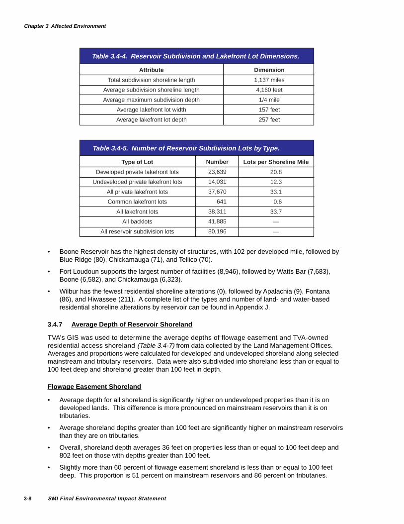
In 1995, subdivisions with lakefront property were randomly sampled to further characterize existingshoreline development. Data on the frequency, types, and dimensions of subdivision lots werecollected from 684 subdivision plats. These data were then expanded to give estimates for all 1,443reservoir subdivisions (Tables 3.4-4 and 3.4-5).
3.4.6 Residential Shoreline Alterations
Development can also be characterized by the number, density, and kinds of residential shorelinealterations along the shoreline (Table 3.4-6). These structures include a wide variety of land- andwater-based facilities but generally consist of fixed and floating piers and docks, retaining walls,decks, patios, steps, riprap, boathouses, etc. A total of 67,692 residential alterations (49 per mile)existed along developed shorelines in 1994.
Chapter 3 Affected Environment
SMI Final Environmental Impact Statement 3-7
% of TotalAvailable forResidential 1
54
63
58
65
51
44
35
60
42
39
13
77
91
54
28
17
19
0
36
14
38
25
36
13
59
0
18
0
0
0
33
Total DevelopedDeveloped Residentia l
Miles
85.9
64.3
184.8
52.1
7.8
25.9
59.9
15.5
141.8
19.4
2.6
87.3
43.2
63.7
17.1
78.1
10.7
0.0
88.7
13.4
18.1
91.0
59.7
120.5
12.0
0.02
19.7
0.02
0.03
0.02
1,383.2
% of TotalShoreline
52
51
49
41
25
25
15
23
20
18
1
10
14
13
9
15
13
0
11
7
10
11
6
6
7
0
6
0
0
0
13
Miles
90.1
67.1
198.6
54.4
10.4
28.5
98.0
17.3
159.2
22.3
47.6
170.5
58.5
91.5
35.4
86.4
12.6
0.7
110.3
24.8
25.0
107.0
87.9
167.5
12.8
8.1
25.5
4.6
10.53
0.0
1,833.1
% of TotalShoreline
54
53
53
43
34
28
25
25
22
21
20
19
19
19
18
17
15
15
14
14
14
13
9
8
8
7
7
6
4
0
17
Total MilesAvailable forResidential 1
157.8
102.6
317.2
79.6
15.4
58.8
172.3
26.0
340.4
50.2
19.3
113.3
47.7
118.3
62.1
454.9
56.4
0.0
248.7
98.0
48.2
360.8
165.4
936.9
20.3
0.0
110.4
11.2
0.0
0.0
4,192.2
TotalShoreline
Miles
166.2
126.6
378.2
128.0
31.0
102.1
394.5
68.1
721.7
104.9
237.8
889.1
308.7
490.6
193.4
512.5
82.3
4.8
783.7
178.7
181.9
809.2
1,027.2
2,064.3
164.8
109.5
357.0
75.1
271.6
31.5
10,995.0
Reservoir
Wilson
Boone
Fort Loudoun
Chatuge
Ft. Patrick Henry
Nottely
Cherokee
Blue Ridge
Watts Bar
Watauga
Fontana
Guntersville
Tims Ford
Pickwick
Melton Hill
Douglas
Beech RiverProject
Wilbur
Chickamauga
Nickajack
South Holston
Norris
Wheeler
Kentucky
Hiwassee
Ocoee Project
Tellico
Normandy
Bear CreekProject
Apalachia
Total Miles
% of Total
Table 3.4-3. Miles of Developed Residential, Total Developed, Total Available for Residential,and Total Shoreline by Reservoir, Ranked by Percentage of Total Shoreline Developed.
1Sum of flowage easement and TVA-owned residential access shoreland.2A negligible amount of residential shoreline development exists.3An undetermined portion of the 10.5 developed shoreline miles is developed for residential use.
Chapter 3 Affected Environment
SMI Final Environmental Impact Statement3-8
Lots per Shoreline Mile
20.8
12.3
33.1
0.6
33.7
—
—
Number
23,639
14,031
37,670
641
38,311
41,885
80,196
Type of Lot
Developed private lakefront lots
Undeveloped private lakefront lots
All private lakefront lots
Common lakefront lots
All lakefront lots
All backlots
All reservoir subdivision lots
Table 3.4-5. Number of Reservoir Subdivision Lots by Type.
• Boone Reservoir has the highest density of structures, with 102 per developed mile, followed byBlue Ridge (80), Chickamauga (71), and Tellico (70).
• Fort Loudoun supports the largest number of facilities (8,946), followed by Watts Bar (7,683),Boone (6,582), and Chickamauga (6,323).
• Wilbur has the fewest residential shoreline alterations (0), followed by Apalachia (9), Fontana(86), and Hiwassee (211). A complete list of the types and number of land- and water-basedresidential shoreline alterations by reservoir can be found in Appendix J.
3.4.7 Average Depth of Reservoir Shoreland
TVA’s GIS was used to determine the average depths of flowage easement and TVA-ownedresidential access shoreland (Table 3.4-7) from data collected by the Land Management Offices.Averages and proportions were calculated for developed and undeveloped shoreland along selectedmainstream and tributary reservoirs. Data were also subdivided into shoreland less than or equal to100 feet deep and shoreland greater than 100 feet in depth.
Flowage Easement Shoreland
• Average depth for all shoreland is significantly higher on undeveloped properties than it is ondeveloped lands. This difference is more pronounced on mainstream reservoirs than it is ontributaries.
• Average shoreland depths greater than 100 feet are significantly higher on mainstream reservoirsthan they are on tributaries.
• Overall, shoreland depth averages 36 feet on properties less than or equal to 100 feet deep and802 feet on those with depths greater than 100 feet.
• Slightly more than 60 percent of flowage easement shoreland is less than or equal to 100 feetdeep. This proportion is 51 percent on mainstream reservoirs and 86 percent on tributaries.
Dimension
1,137 miles
4,160 feet
1/4 mile
157 feet
257 feet
Attribute
Total subdivision shoreline length
Average subdivision shoreline length
Average maximum subdivision depth
Average lakefront lot width
Average lakefront lot depth
Table 3.4-4. Reservoir Subdivision and Lakefront Lot Dimensions.
Chapter 3 Affected Environment
SMI Final Environmental Impact Statement 3-9
Number of Alterations
Per Developed Mile ofResidential Shoreline
—
NA
NA
80
102
44
16
71
24
33
48
68
67
18
42
58
51
NA
19
42
—
45
60
70
48
43
54
60
0
44
49
Land-Based
—
NA
NA2
513
2,209
1,087
216
1,361
698
21
2,244
154
2,523
76
1,611
297
123
NA2
455
586
—
566
649
413
819
510
1,733
1,160
0
63
20,087
Water-Based
—
NA
NA
720
4,373
1,226
756
4,962
1,203
65
6,702
375
3,315
135
3,423
697
555
NA
1,258
497
—
2,292
429
961
1,268
321
5,950
2,436
0
3,686
47,605
Total
—
NA
NA
1,233
6,582
2,313
972
6,323
1,901
86
8,946
529
5,838
211
5,034
994
678
NA
1,713
1,083
—
2,858
1,078
1,374
2,087
831
7,683
3,596
0
3,749
67,692
Table 3.4-6. Number of Land- and Water-Based Residential Shoreline Alterationsby Reservoir.
Reservoir
Apalachia1
Bear Creek Project
Beech River Project
Blue Ridge
Boone
Chatuge
Cherokee
Chickamauga
Douglas
Fontana
Fort Loudoun
Fort Patrick Henry
Guntersville
Hiwassee
Kentucky
Melton Hill
Nickajack
Normandy
Norris
Nottely
Ocoee Project1
Pickwick
South Holston
Tellico
Tims Ford
Watauga
Watts Bar
Wheeler
Wilbur
Wilson
Total
2
1The shoreline area is managed by TVA and other agencies for purposes other than residential access. A few residentialalterations exist as a result of special use permits, but these are not included in the total.
All ShorelandDeveloped Undeveloped All ShorelandDeveloped Undeveloped
ShorelandDepth Classification
29
947
497
49
51
40
317
87
83
17
33
889
400
57
43
32
867
441
51
49
41
279
75
86
14
36
802
331
61
39
55
314
148
60
40
54
206
71
80
20
55
294
122
66
34
47
357
165
58
42
54
472
231
50
50
50
419
199
54
46
51
337
157
59
41
54
431
181
59
41
52
377
167
59
41
Reservoirs
Shoreland <100 ft.
Shoreland >100 ft.
All Shoreland
Shoreland <100 ft.
Shoreland >100 ft.
All Reservoirs
Shoreland <100 ft.
Shoreland >100 ft.
All Shoreland
Shoreland <100 ft.
Shoreland >100 ft.
42
551
256
58
42
43
205
61
89
11
43
492
169
72
28
Table 3.4-7. Average Shoreland Depth by Reservoir Group, Depth Classification, andDevelopment Status for Two Ownership Categories.
MainstreamReservoirs
Shoreland <100 ft.
Shoreland >100 ft.
All Shoreland
Shoreland <100 ft.
Shoreland >100 ft.
Tributary
Average Depth (ft.)
Percent
Average Depth (ft.)
Average Depth (ft.)
Percent
Percent
1Averages based on data collected on 4 mainstream and 9 tributary reservoirs.2Averages based on data collected on 7 mainstream and 13 tributary reservoirs.
TVA-Owned Residential Access Shoreland
• Average depth of all TVA-owned residential access shoreland is significantly higher on undevelopedproperties than it is on developed lands. The difference is much more pronounced on tributariesthan on mainstream reservoirs.
• When compared to mainstream reservoirs, average shoreland depths greater than 100 feet arehigher on undeveloped tributary reservoir shoreland but lower on developed properties.
• Average depths of shoreland less than or equal to 100 feet in depth are about equal betweendeveloped and undeveloped properties and also between mainstream and tributary reservoirs.
• Overall, TVA-owned residential access shoreland depth averages 52 feet on properties less thanor equal to 100 feet deep and 377 feet on those with depths greater than 100 feet.
• Almost 60 percent of shoreland in this ownership category is less than or equal to 100 feet deep.This proportion is the same on mainstream and tributary reservoirs.
Chapter 3 Affected Environment
SMI Final Environmental Impact Statement 3-11
3.5 Shoreline V egetation
3.5.1 Introduction
Almost all of the reservoir shoreline and study area is vegetated with some combination of trees, shrubs,forbs, and grasses. Forest is the principal land cover type. Based on an analysis of late successionalforests, Braun (1950) described four forest regions in the Tennessee River drainage basin:
The first three of these regions are primarily composed of deciduous trees, with conifers restricted toparticular conditions such as dry ridges and early successional stages of forest development.
With the demise of American chestnut (about 1930), the Oak-Chestnut Forest Region is nowcharacterized by several species of oak, with yellow-poplar, maple, and American beech common onmore moist sites. This region includes the Blue Ridge and most of the Valley and Ridge physiographicprovinces (Fenneman, 1938) (Figure 3.5-1).
The Cumberland Plateau Physiographic Province is within the Mixed Mesophytic Forest Region. Thisregion is characterized by numerous tree species which share dominance. Common dominant speciesinclude tuliptree, basswood, sugar maple, buckeye, northern red oak, white oak, and white ash.
The rest of the Tennessee Valley, including the Highland Rim, Nashville Basin, and eastern portion ofthe Coastal Plain Physiographic Provinces, is in the Western Mesophytic Forest Region. Its forestsare less diverse than those of the Mixed Mesophytic region and are characterized by several speciesof oaks, hickories, maples, and elms.
A small portion of the Valley and Ridge and Coastal Plain Provinces, along the southern border of theTennessee Valley, lies within the Oak-Pine Forest Region. This region is characterized by a mixture ofseveral species of oaks, hickories, and shortleaf and loblolly pines.
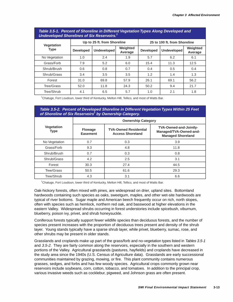
3.5.2 Shoreline V egetation T ypes
Vegetation types along reservoir shorelines were surveyed on six reservoirs (Table 3.5-1), asdescribed in Section 3.8.9 and Appendix K. The proportions of most vegetation types within 25 feetof the shoreline and 25 to 100 feet from the shoreline are similar. Within each distance zone, theproportions of forest (called the tree category in Section 3.8.9 and Appendix K) and tree/grass categoriesdiffer significantly (chi-square tests, P < 0.05) between developed and undeveloped shorelines. Mostof the tree/grass vegetation type is open woodland with a mowed understory typical of wooded yards.The forest category is comparatively undisturbed woodland.
The proportions of the major vegetation types along developed shorelines also vary between ownershipcategories (Table 3.5-2). Compared to TVA-owned residential access shoreland, flowage easementshoreland has a higher proportion in the grass/forb category and a lower proportion in the combinedtree-dominated categories (forest, tree/grass, and tree/shrub). These differences are due in part tolimited vegetative management on TVA-owned residential access shoreland (Section 1.4.5).
The species composition of study area forests varies greatly within Braun’s (1950) regions because ofvariation in elevation, relief, soil fertility, moisture, and history of human disturbance. Young to mid-successional forests tend to have fairly similar species composition on sites with similar environmen-tal conditions. Eastern redcedar and mixed cedar types are common on reverting old fields and onsites with shallow soils over limestone. Pines are widespread and occur both naturally in earlysuccessional stands and in plantations. Loblolly pine plantations are fairly common along reservoirshorelines, especially in the southern and western portions of the Valley.
Chapter 3 Affected Environment
SMI Final Environmental Impact Statement3-12
Tenn
esse
e R
iver
Wat
ersh
ed10
020
4060
100
2040
1. B
lue
Rid
ge4.
Hig
hlan
d R
im2.
Val
ley
and
Rid
ge5.
Nas
hvill
e B
asin
3. C
umbe
rlan
d P
late
au6.
Coa
stal
Pla
in
Fig
ure
3.5
-1.
Phy
sio
gra
ph
ic P
rovi
nce
s o
f th
e Te
nn
esse
e Va
lley.
Chapter 3 Affected Environment
SMI Final Environmental Impact Statement 3-13
WeightedAverage
Table 3.5-1. Percent of Shoreline in Different Vegetation Types Along Developed andUndeveloped Shorelines of Six Reservoirs. 1
VegetationType
25 to 100 ft. from ShorelineUp to 25 ft. from Shoreline
WeightedAverageDeveloped Undeveloped Developed Undeveloped
No Vegetation
Grass/Forb
Shrub/Brush
Shrub/Grass
Forest
Tree/Grass
Tree/Shrub
1.0
7.9
0.6
3.4
31.0
52.0
4.1
6.1
12.5
0.4
1.3
56.2
21.7
1.8
6.2
11.3
0.5
1.4
69.1
9.4
2.1
5.7
15.4
0.4
1.2
26.1
50.2
1.0
1.9
6.0
0.7
3.5
57.9
24.3
5.7
2.4
5.2
0.8
3.5
69.8
11.8
6.51Chatuge, Fort Loudoun, lower third of Kentucky, Melton Hill, Tellico, and most of Watts Bar.
Oak-hickory forests, often mixed with pines, are widespread on drier, upland sites. Bottomlandhardwoods containing such species as oaks, sweetgum, maples, and other wet-site hardwoods aretypical of river bottoms. Sugar maple and American beech frequently occur on rich, north slopes,often with species such as hemlock, northern red oak, and basswood at higher elevations in theeastern Valley. Widespread shrubs occurring in forest understories include spicebush, viburnum,blueberry, poison ivy, privet, and shrub honeysuckle.
Coniferous forests typically support fewer wildlife species than deciduous forests, and the number ofspecies present increases with the proportion of deciduous trees present and density of the shrublayer. Young stands typically have a sparse shrub layer, while privet, blueberry, sumac, rose, andother shrubs may be present in older stands.
Grasslands and croplands make up part of the grass/forb and no-vegetation types listed in Tables 3.5-1and 3.5-2. They are fairly common along the reservoirs, especially in the southern and westernportions of the Valley. Agricultural grasslands (pastures, hayfields) and croplands have decreased inthe study area since the 1940s (U.S. Census of Agriculture data). Grasslands are early successionalcommunities maintained by grazing, mowing, or fire. This plant community contains numerousgrasses, sedges, and forbs and has few woody species. Agricultural crops commonly grown nearreservoirs include soybeans, corn, cotton, tobacco, and tomatoes. In addition to the principal crop,various invasive weeds such as cocklebur, pigweed, and Johnson grass are often present.
Ownership Category
VegetationType
No Vegetation
Grass/Forb
Shrub/Brush
Shrub/Grass
Forest
Tree/Grass
Tree/Shrub1Chatuge, Fort Loudoun, lower third of Kentucky, Melton Hill, Tellico, and most of Watts Bar.
TVA-Owned-and-Jointly-Managed/TVA-Owned-and-
Managed Shoreland
TVA-Owned ResidentialAccess Shoreland
FlowageEasement
0.7
9.3
0.7
4.2
30.3
50.5
4.3
0.3
4.8
0.3
2.5
27.4
61.6
3.1
3.9
11.8
0.8
3.1
44.5
29.3
6.6
Table 3.5-2. Percent of Developed Shoreline in Different Vegetation Types Within 25 Feetof Shoreline of Six Reservoirs 1 by Ownership Category.
Chapter 3 Affected Environment
SMI Final Environmental Impact Statement3-14
Brushlands are areas dominated by shrubs and saplings and include the shrub/brush and part of theshrub/grass types listed in Table 3.5-1. They are less common near reservoirs than are forests andgrasslands, and their area has decreased since the 1940s (U.S. Census of Agriculture data). Brush-lands include abandoned farmlands in the early stages of reverting to forest, as well as recentlyclearcut forests. Blackberry, persimmon, sassafras, and numerous native and nonnative herbs arewidespread in brushlands. Without periodic mowing or burning, brushlands eventually revert to forest.
The plant communities of urban and suburban areas vary greatly and include portions of all theshoreline vegetation types listed in Table 3.5-1. The vegetation types and species present areaffected by the density of development, previous land use, amount of clearing, and type of landscap-ing. Extensive areas of mowed lawns are common, and trees and shrubs often occur in clumps or asscattered individuals. Tree species present often include such natives as pin oak, sycamore,sweetgum, flowering dogwood, and maples, as well as planted and invasive nonnative species suchas tree-of-heaven, Bradford pear, ginkgo, and mimosa.
3.5.3 Forest Area and T ract Size
Forest covers 55.1 percent (standard deviation = 18.6) of the area1 of the 67 counties adjoining TVAreservoirs. This contrasts with the area within one-fourth mile of the reservoir shoreline, which is 67.4percent (standard deviation = 18.5) forested; the difference in these two proportions is significant(paired T-test, P < 0.01). When analyzed county by county, the proportion of forested land within one-fourth mile of the shoreline correlated poorly with the proportion for the whole county. This suggeststhat land use patterns adjacent to a reservoir are often different from those of surrounding counties.In many counties with a low proportion (e.g., less than one-third) of forested land, forests within one-fourth mile of the shoreline made up a disproportionately large amount of the total forested area.These counties are dominated by agricultural and urban land uses and include Limestone, Alabama,and Hamblen, Loudon, Meigs, and Union, Tennessee. All of these counties have at least 20 percentof their forest area within one-fourth mile of reservoir shorelines.
The proportion of forested land within the study area increased by about 8 percent between 1940 and1980 (USDA Forest Service, Forest Inventory and Analysis data). This increase, due mostly to thereforestation of abandoned farmland, has slowed in recent years; since 1980, forest cover hasincreased about 0.4 percent. Quantitative information on the trend in the proportion of forested landwithin one-fourth mile of the reservoir shorelines is not available. The current proportion of forestedland within this zone, however, is weakly correlated with the age of the reservoir. Extrapolating fromthis relationship to a trend, however, is difficult because of varying land ownership patterns, physi-ographic settings, and local population densities.
Both the proportion of forested land and the size of contiguous tracts of forest within the one-fourth-mileshoreline zone are related to the development status of the reservoir shoreline. Analysis of ninereservoirs2 showed that 53.1 percent of this zone is in forest. The proportion of forested land issignificantly greater (paired T-test, P = 0.01) along undeveloped shorelines (average 54.2, standarddeviation = 15.0) than along developed shorelines (average 42.8, standard deviation = 16.2) on areservoir-by-reservoir basis. Contiguous tracts of forest within this zone average 18.2 acres in size.3
Along undeveloped shorelines, contiguous tracts of forest average 24.6 acres (standard deviation =17.9), significantly greater (paired T-test, P < 0.05) than the average of 10.5 acres (standard deviation= 5.1) along developed shorelines.
1Determined from interpreted 1989-1992 LANDSAT satellite imagery with a minimum resolution (pixel size) of approxi-mately 100 by 100 feet.
2Chatuge, Chickamauga, Fort Loudoun, lower one-third of Kentucky, Melton Hill, Norris, Tellico, Watts Bar, and Wheeler;determined from interpreted 1989-1992 LANDSAT satellite imagery with a minimum resolution (pixel size) of approximately 100by 100 feet.
3Determined from LANDSAT forest cover data after overlaying 150-foot-wide unforested buffer along primary roads and75-foot-wide unforested buffer along secondary roads. Because of the one-fourth-mile zone limits, tract sizes are underesti-mated; some extended further from the shoreline.
Chapter 3 Affected Environment
SMI Final Environmental Impact Statement 3-15
3.6 Wildlife
3.6.1 Introduction
Because it includes portions of six physiographic regions (Fenneman, 1938) (Figure 3.5-1) and manydifferent plant communities, the reservoir area and adjacent counties support a large number ofwildlife species, including about 500 species of vertebrates other than fish. Many of these animalsare conspicuous parts of the shoreline environment.
3.6.2 Forest W ildlife Populations
This section describes the wildlife found in the upland forests of the study area. Wildlife speciesfound in forested wetlands are listed in Appendix L.
Deciduous forests support the greatest diversity of wildlife. Common mammals in this type includethe red bat, short-tailed shrew, gray squirrel, and white-footed mouse. The bird community includesspecies present throughout the year, species which nest in the region and migrate to winter in theCaribbean and Latin America (often referred to as neotropical migrants), and species which winter inthe region. Common birds present throughout the year include woodpeckers, the blue jay, Carolinachickadee, tufted titmouse, and Carolina wren. Common neotropical migrants include the yellow-billed cuckoo, wood thrush, red-eyed vireo, Kentucky and hooded warblers, and summer tanager.Wintering birds include the winter wren, gold-crowned kinglet, and yellow-rumped warbler. Among thecommon reptiles are the five-lined skink, eastern box turtle, and ringneck and rat snakes. Commonamphibians, especially near water, are the American toad, spring peeper, and dusky and slimysalamanders. The number of wildlife species present tends to increase with the size of theforested area. This has been especially well documented for neotropical migrant birds (e.g.,Robbins et al., 1989).
Coniferous forests typically support fewer wildlife species than deciduous forests, and the number ofspecies present increases with the proportion of deciduous trees present and the density of the shrublayer. The pine warbler, ground skink, and southeastern crowned snake are among the few speciesfrequently found in pine forests across the Valley. Several of the species found in deciduous forestsalso occur in mixed coniferous-deciduous forests, and several species found in dry, upland pines alsooccur in dry, upland, deciduous forests.
Several common game animals occur in shoreline forests. The gray squirrel and ruffed grouse occurprimarily in forests. White-tailed deer and wild turkey occur in deciduous and coniferous forests andalso use adjacent grassland, cropland, and brushland habitats. With the exception of the ruffedgrouse, these species occur around most TVA reservoirs. Ruffed grouse are restricted to forests inthe eastern end of the Valley. Harvest surveys and census results compiled by state wildlife agenciesshow that populations of both white-tailed deer and wild turkey are generally increasing. Gray squirreland ruffed grouse populations appear relatively stable.
Information on the population trends of other forest wildlife is only available for birds at the regionalscale. North American Breeding Bird Survey results for 1966-1994 show significant (P < 0.10) in-creasing or decreasing trends (analyzed as described by Link and Sauer, 1994) in 20 birds nesting inValley forests. For those species requiring extensive tracts of forest, the proportion with decreasingtrends is significantly greater (chi-square test, P < 0.01) than the proportion with increasing trends.The proportion of neotropical migrants with decreasing trends is also greater than the proportion withincreasing trends. There are no significant differences in these proportions for permanent residentsor species nesting in small tracts of forest.
3.6.3 Wintering W aterfowl Populations
TVA reservoirs provide migration and winter habitat for many waterfowl species. On a continentalbasis, they are very important to Canada geese, mallards, American black ducks, American
Chapter 3 Affected Environment
SMI Final Environmental Impact Statement3-16
widgeons, and gadwalls, as well as to migrating blue-winged teal, northern pintails, ring-neckedducks, and lesser scaup (Bellrose, 1980).
Since the 1930s, numerous actions designed to increase the suitability of TVA reservoirs for waterfowlhave been carried out (Wiebe, 1946; Wiebe et al., 1950). These actions have included establishingtwo national wildlife refuges and numerous state wildlife refuges and management areas, constructingsubimpoundments, operating dewatering areas, and planting food crops. Wildlife refuges and man-agement areas presently make up a large percentage of the TVA-owned-and-jointly-managed shore-land.
The population trends of waterfowl vary among species. The number of migrant Canada geesewintering in the Valley has decreased since the 1960s, as they have shifted their wintering groundsnorthward. Nonmigratory Canada geese have greatly increased in the Valley since stocking programsbegan in the 1970s, and on some reservoirs these geese have become nuisances. Wood ducknumbers have increased as shoreline forests matured, resulting in more suitable nest sites, and asincreasing beaver populations created more suitable wetlands habitats. Populations of most otherducks have shown a long-term decrease consistent with their continental trends. Local populations ofseveral ducks such as the gadwall and American widgeon fluctuate with the availability of aquatic bedwetlands (Section 3.9.3).
To quantitatively describe the quality of reservoir areas for wintering waterfowl populations, awaterfowl habitat suitability model was developed. This model focuses on dabbling ducks, such asthe mallard, American black duck, American widgeon, and gadwall, which frequent shallow water andshoreline areas.
The major components of the model are the presence and diversity of wetlands, the degree of humandisturbance along the shoreline (based on the type of shoreline development), and the proximity towildlife refuges and management areas. Another important habitat component, the proximity tocroplands of cultivated grains, notably corn (Allen, 1986; Johnson and Montalbano, 1989), was notincluded because current maps showing their distribution were not available. The model was appliedto Chatuge, Chickamauga, Tellico, Watts Bar, and the downstream third of Kentucky Reservoirs.Within each reservoir, the area of analysis was the drawdown zone between the normal summer andwinter pool levels. Habitat quality was scored on a scale from 0, indicating low suitability, to 3, thehighest suitability. A detailed description of the model is given in Appendix M.
Existing Conditions
The drawdown zone of each reservoir was divided into three suitability classes. Thirty-five percent ofthe area was classified as low suitability (score 0-1), 41 percent as moderate suitability (score 1-2),and 24 percent as high suitability (score 2-3) wintering waterfowl habitat (Figure 3.6-1). The draw-down zone fronting developed shoreline has a higher proportion of low suitability habitat and a lowerproportion of both moderate and high suitability habitat than the drawdown zone fronting undevelopedshoreline. The differences in the proportions of developed and undeveloped shoreline in the low andhigh suitability classes are significant (paired T-test, P < 0.01 and P = 0.02, respectively). The differ-ence in the proportion of developed and undeveloped shoreline in the moderate suitability classapproaches significance (P = 0.06). Much of the difference is due to increased human disturbancealong developed shorelines. The lower frequency of wetlands occurrence near developed shorelines(Section 3.9.5) was also a factor.
3.6.4 Other W ildlife Communities
Grasslands and croplands support few wildlife species. Common species present in grasslandsinclude the eastern meadowlark, red-winged blackbird, rat snake, eastern garter snake, and Fowler’stoad. Species commonly occurring in croplands include the common grackle, red-winged blackbird,black racer, eastern garter snake, and Fowler’s toad. Several of these species feed in croplands butrequire other habitats for breeding.
Chapter 3 Affected Environment
SMI Final Environmental Impact Statement 3-17
Brushlands support wildlife populations with diversity intermediate between those of deciduous forestsand grasslands. Common species include the cotton rat, white-eyed vireo, common yellowthroat,yellow-breasted chat, indigo bunting, field sparrow, black racer, fence lizard, and Fowler’s toad.
North American Breeding Bird Survey results show declining population trends since 1966 for themajority of grassland and brushland birds. This declining trend is occurring in both permanentresident and neotropical migrant species and is in part due to the decrease in grassland and brush-land habitats. Little population trend information is available for other animals occurring in grasslandsand brushlands.
The eastern cottontail and northern bobwhite are common game species which use grasslands,croplands, and brushlands. Another common game species, the mourning dove, frequently feeds incroplands. Area populations of the cottontail and bobwhite are decreasing, while mourning dovepopulations appear relatively stable.
Urban and suburban areas vary in their wildlife populations, depending on the density of development,previous land use, amount of clearing, and type of landscaping. Species present in areas withextensive lawns and few trees include both nonnative species such as the house mouse, rock dove,European starling, and house finch, and native species such as the American robin and northernmockingbird. The nonnative house finch and native gray squirrel, mourning dove, chimney swift,northern cardinal, and eastern garter snake occur in urban and suburban areas over a wide range ofvegetation density. Several of the wildlife species present in deciduous and coniferous forests occurin suburban areas that have a high proportion of forest cover.
In addition to waterfowl, a variety of shorebirds and other waterbirds use Valley reservoirs.Shorebirds (mostly sandpipers and plovers) are most numerous during their spring and late summer/early fall migration periods and prefer very shallow water (less than 3 inches deep) and moist areaswithin the drawdown zone. Their numbers in reservoir habitats vary with seasonal weather patternsand reservoir drawdown regimes. Other waterbirds present include the double-crested cormorant,great blue heron, great egret, black-crowned night heron, and osprey. Populations of these specieswithin the reservoir area have greatly increased since the 1940s as a result of expansion into newlycreated habitat, recovery from pesticide poisoning, and responses to specific management actions(Beddow, 1990; Pullin, 1990; Palmer-Ball, 1991).
Moderate High
Score
0
Per
cent
Developed
Undeveloped
Total
Figure 3.6-1. Wintering Waterfowl Habitat Suitability in Relation to Shoreline Development.
75.9
23.9
35.0
23.8
45.741.0
Low
0.3
30.424.0
10
20
30
40
50
60
70
80
90
100
Chapter 3 Affected Environment
SMI Final Environmental Impact Statement3-18
3.7 Endangered and Threatened Species
The Endangered Species Act of 1973, as amended,
• Establishes procedures for identifying animal and plant species in need of protection.
• Requires all federal agencies to determine if their activities are likely to jeopardize the continuedexistence of listed species.
• Requires federal agencies to cooperate in programs for the conservation of listed species.
• Sets penalties for illegal taking, possession, or sale of listed species, their parts, or products.
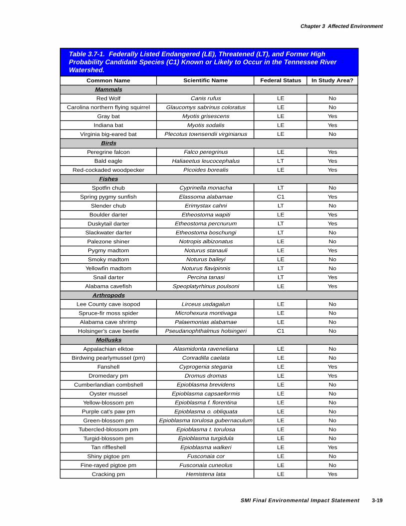
Information presented in the most recent USF&WS listing of endangered and threatened species(USF&WS, 1994) and records maintained in TVA’s Natural Heritage database indicate that a numberof listed and well-studied candidate plant and animal species occur, or have occurred, in the Tennes-see River watershed. The names and listing status of these species are presented in Table 3.7-1,along with listed species that occur within the area potentially impacted, either directly, indirectly, orcumulatively, by the various shoreline management alternatives. This study area is considered to bethe shoreline and pools of TVA reservoirs, the land area extending about 3 miles from the shoreline,the tailwaters downstream of the dams, and the lower stretches of tributary streams within about 3miles of reservoir pools. The 3-mile distance was used to better account for the distributions, biology,and home ranges of the different listed species.
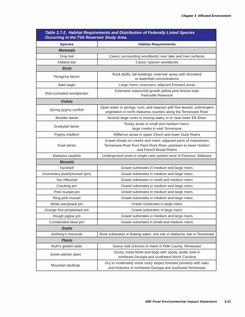
Table 3.7-2 lists the habitat requirements of the 25 species in this study area. These species varygreatly in their distribution in the reservoir area. The three plant species and one of the bird speciesoccur in a small portion of the region. The remaining four terrestrial species, two bats and two birds,are relatively widespread.
Two of the 17 aquatic species included in Table 3.7-2 occur in relatively unique habitats: undergroundpools for the Alabama cavefish, and low gradient, open water pools with submergent vegetation forthe spring pygmy sunfish. Most of the other federally protected aquatic species potentially affected byshoreline management alternatives occur downstream from dams where important habitat conditionspersist. Several of these species typically occur together as parts of diverse communities in placessuch as the Tennessee River downstream from Pickwick Landing Dam or the Elk River, a consider-able distance downstream from Tims Ford Dam. Populations of several of these species also surviveupstream from some reservoirs (on stream reaches) and would not be affected by reservoir shorelinemanagement decisions.
3.8 Soils
3.8.1 Introduction
The Tennessee Valley is a diverse area made up of six different physiographic provinces (Fenneman,1938) (Figure 3.5-1). These range from the rugged Blue Ridge Mountains in the eastern portion ofthe Valley region to the flat coastal plain area in the western portion. Variations in factors such astopography, climate, and parent material account for the development of different soils within eachprovince. These soils range from shallow and loamy to deep clay.
3.8.2 Climate
The Tennessee Valley has a warm, temperate, humid climate. Most of the Valley receives 46 to 54inches of rainfall annually. The Blue Ridge province is cooler and wetter due to the higher elevations,with rainfall averaging 54 to 80 inches annually in the Unaka Mountains. The Cumberland Mountains,located in the Cumberland Plateau province, receive 54 to 60 inches of precipitation annually, alsodue to the higher elevation. Rainfall of this amount influences soil erosion potential. Average annualtemperature varies from 62oF in the southwest portion of the Tennessee Valley region to 45oF in thehigh mountain peaks of the Unakas.
Chapter 3 Affected Environment
SMI Final Environmental Impact Statement 3-19
Common Name
Mammals
Red Wolf
Carolina northern flying squirrel
Gray bat
Indiana bat
Virginia big-eared bat
Birds
Peregrine falcon
Bald eagle
Red-cockaded woodpecker
Fishes
Spotfin chub
Spring pygmy sunfish
Slender chub
Boulder darter
Duskytail darter
Slackwater darter
Palezone shiner
Pygmy madtom
Smoky madtom
Yellowfin madtom
Snail darter
Alabama cavefish
Arthropods
Lee County cave isopod
Spruce-fir moss spider
Alabama cave shrimp
Holsinger’s cave beetle
Mollusks
Appalachian elktoe
Birdwing pearlymussel (pm)
Fanshell
Dromedary pm
Cumberlandian combshell
Oyster mussel
Yellow-blossom pm
Purple cat’s paw pm
Green-blossom pm
Tubercled-blossom pm
Turgid-blossom pm
Tan riffleshell
Shiny pigtoe pm
Fine-rayed pigtoe pm
Cracking pm
Scientific Name
Canis rufus
Glaucomys sabrinus coloratus
Myotis grisescens
Myotis sodalis
Plecotus townsendii virginianus
Falco peregrinus
Haliaeetus leucocephalus
Picoides borealis
Cyprinella monacha
Elassoma alabamae
Erimystax cahni
Etheostoma wapiti
Etheostoma percnurum
Etheostoma boschungi
Notropis albizonatus
Noturus stanauli
Noturus baileyi
Noturus flavipinnis
Percina tanasi
Speoplatyrhinus poulsoni
Lirceus usdagalun
Microhexura montivaga
Palaemonias alabamae
Pseudanophthalmus holsingeri
Alasmidonta raveneliana
Conradilla caelata
Cyprogenia stegaria
Dromus dromas
Epioblasma brevidens
Epioblasma capsaeformis
Epioblasma f. florentina
Epioblasma o. obliquata
Epioblasma torulosa gubernaculum
Epioblasma t. torulosa
Epioblasma turgidula
Epioblasma walkeri
Fusconaia cor
Fusconaia cuneolus
Hemistena lata
Federal Status
LE
LE
LE
LE
LE
LE
LT
LE
LT
C1
LT
LE
LT
LT
LE
LE
LE
LT
LT
LE
LE
LE
LE
C1
LE
LE
LE
LE
LE
LE
LE
LE
LE
LE
LE
LE
LE
LE
LE
In Study Area?
No
No
Yes
Yes
No
Yes
Yes
Yes
No
Yes
No
Yes
Yes
No
No
Yes
No
No
Yes
Yes
No
No
No
No
No
No
Yes
Yes
No
No
No
No
No
No
No
Yes
No
No
Yes
Table 3.7-1. Federally Listed Endangered (LE), Threatened (LT), and Former HighProbability Candidate Species (C1) Known or Likely to Occur in the Tennessee RiverWatershed.
Chapter 3 Affected Environment
SMI Final Environmental Impact Statement3-20
Table 3.7-1 (Cont.). Federally Listed Endangered (LE), Threatened (LT), and FormerHigh Probability Candidate Species (C1) Known or Likely to Occur inthe Tennessee River Watershed.
In Study Area?
Yes
No
Yes
No
Yes
Yes
No
Yes
No
No
No
No
No
No
Yes
No
Yes
No
No
No
No
No
No
No
No
No
No
No
No
No
No
Yes
No
No
No
Yes
No
Yes
No
No
Scientific Name
Lampsilis abrupta
Lampsilis virescens
Obovaria retusa
Pegias fabula
Plethobasus cicatricosus
Plethobasus cooperianus
Pleurobema clava
Pleurobema plenum
Quadrula cylindrica strigillata
Quadrula fragosa
Quadrula intermedia
Quadrula sparsa
Toxolasma cylindrellus
Villosa perpurpurea
Villosa trabilis
Anguispira picta
Athearnia anthonyi
Pyrgulopsis ogmorhaphe
Mesodon clarki nantahala
Apios priceana
Betula uber
Clematis morefieldii
Conradilla verticillata
Dalea foliosa
Geum radiatum
Helianthus eggertii
Helonias bullata
Isotria medeoloides
Lesquerella lyrata
Marshallia mohrii
Phyllitis scolopendrium var.americanum
Pityopsis ruthii
Ptilimnium nodosum
Sagittaria fasciculata
Sagittaria secundifolia
Sarracenia oreophila
Sarracenia rubra ssp. jonesii
Scutellaria montana
Solidago spithamaea
Xyris tennesseensis
Federal Status
LE
LE
LE
LE
LE
LE
LE
LE
LE
LE
LE
LE
LE
LE
LE
LT
LE
LE
LT
LT
LT
LE
LT
LE
LE
LT
LT
LT
LT
LT
LE
LE
LE
LE
LT
LE
LE
LE
LT
LE
Common Name
Mollusks (cont.)
Pink mucket pm
Alabama lampshell
Ring pink mussel
Little-wing pm
White wartyback pm
Orange-foot pimpleback pm
Clubshell
Rough pigtoe pm
Rough rabbitsfoot (mussel)
Winged mapleleaf mussel
Cumberland monkeyface pm
Appalachian monkeyface pm
Pale lilliput pm
Purple bean
Cumberland bean pm
Snails
Painted snake coiled forest snail
Anthony’s riversnail
Royal marstonia (snail)
Noonday globe
Plants
Price potato-bean
Virginia roundleaf birch
Morefield’s leather flower
Cumberland rosemary
Prairie clover
Spreading avens
Eggert sunflower
Swamp pink
Small whorled pogonia
Lyre-leaf bladderpod
Barbara buttons
American harts-tongue fern
Ruth’s golden aster
Harperella
Arrowhead
Arrowhead
Green pitcher plant
Mountain sweet pitcher plant
Mountain skullcap
Blue Ridge goldenrod
Yellow-eyed-grass
Chapter 3 Affected Environment
SMI Final Environmental Impact Statement 3-21
Species
Mammals
Gray bat
Indiana bat
Bir ds
Habitat Requirements
Caves; surrounding woodlands; over lake and river surfaces
Caves; riparian woodlands
Rock bluffs; tall buildings; reservoir areas with shorebirdor waterfowl concentrations
Large rivers; reservoirs; adjacent forested areas
Extensive mature/old growth yellow pine forests nearParksville Reservoir
Open water in springs, runs, and swamps with fine-leaved, submergentvegetation in north Alabama counties along the Tennessee River
Around large rocks in moving water, in or near lower Elk River
Rocky areas in small and medium rivers;large creeks in east Tennessee
Riffle/run areas in upper Clinch and lower Duck Rivers
Gravel shoals on creeks and rivers; adjacent parts of mainstreamTennessee River from Paint Rock River upstream to lower Holston
and French Broad Rivers
Underground pools in single cave system west of Florence, Alabama
Gravel substrates in medium and large rivers
Gravel substrates in medium and large rivers
Gravel substrates in small and medium rivers
Gravel substrates in medium and large rivers
Gravel substrates in medium and large rivers
Gravel substrates in medium and large rivers
Gravel substrates in large rivers
Gravel substrates in large rivers
Gravel substrates in medium and large rivers
Gravel substrates in small and medium rivers
Rock substrates in flowing water; one site in Alabama, two in Tennessee
Sunny rock crevices in rivers in Polk County, Tennessee
Sunny, moist fields and bogs with sandy, acidic soils innortheast Georgia and southwest North Carolina
Dry to moderately moist rocky slopes forested primarily with oaksand hickories in northwest Georgia and southeast Tennessee
Peregrine falcon
Bald eagle
Red-cockaded woodpecker
Fishes
Spring pygmy sunfish
Boulder darter
Duskytail darter
Pygmy madtom
Snail darter
Alabama cavefish
Mussels
Fanshell
Dromedary pearlymussel (pm)
Tan riffleshell
Cracking pm
Pink mucket pm
Ring pink mussel
White wartyback pm
Orange foot pimpleback pm
Rough pigtoe pm
Cumberland bean pm
Snails
Anthony’s riversnail
Plants
Ruth’s golden aster
Green pitcher plant
Mountain skullcap
Table 3.7-2. Habitat Requirements and Distribution of Federally Listed SpeciesOccurring in the TVA Reservoir Study Area .
Chapter 3 Affected Environment
SMI Final Environmental Impact Statement3-22
3.8.3 Soils of the Blue Ridge
The Blue Ridge physiographic province is located in extreme eastern Tennessee, western NorthCarolina, and portions of northern Georgia. Ten TVA reservoirs are located in this easternmostprovince of the Tennessee Valley (Table 3.8-1). Elevations range from 100 to over 6,000 feet. Collu-vium, which is material carried down slopes by gravity, is the parent material for soils found from thefootslopes almost to the ridges. The loamy soils on the upper slopes of the mountains are about 1 to3 feet thick over rock and contain various amounts of rock fragments. The soils gradually becomedeeper (3 to 7 feet) farther down the slope. The valley soils are deep, well-drained, and loamy. Thesoils of the Unaka Mountains region are not highly erodible due to the loamy texture and high organiccontent, but erosion can be a major problem on steep slopes where woody vegetation has beencleared.
3.8.4 Soils of the V alley and Ridge
The Valley and Ridge physiographic province is located west of the Blue Ridge province and east ofthe Cumberland Plateau. It extends from southwest Virginia, through eastern Tennessee, and intonorthern Georgia and Alabama. Ten TVA reservoirs are located in this province, which has elevationsranging from 600 to 3,000 feet. The region is underlain by steeply tilted and folded rock formationsextending in a northeast to southwest direction. The parent materials for the soils on the ridges aresandstone and hard shale, with some formed from cherty, dolomitic limestone. Soft shales andlimestones intermixed with clay, along with colluvium from the upland slopes, form the parent materialin the valleys. The soils are generally shallow over the shales and sandstones and very deep over thedolomitic limestone. Due to clay and the loamy texture, erosion potential is low for these soils, excepton slopes without adequate vegetative cover.
3.8.5 Soils of the Cumberland Plateau
The Cumberland Plateau physiographic province is located east of the Highland Rim and west of theValley and Ridge Province. It extends from southwestern Virginia through east central Tennessee intonortheastern Alabama. Two TVA reservoirs are located in this province, which has elevations rangingfrom 600 feet in the valleys to 3,000 feet in the northeast mountains. The parent materials underlyingthis area are Pennsylvanian sandstone and shales. Soils in the valleys also formed from alluvium andcolluvium, which had weathered and moved downslope. The dominant soils in this region range from2 to 4 feet deep over rock. Sandstone outcroppings are common on slopes. Plateau soils are loamyin texture, which usually means a low erosion potential. However, shallow soil depth, rock content,and steep slopes result in slippage and subsequent erosion problems.
3.8.6 Soils of the Highland Rim
The Highland Rim physiographic province is located west of the Cumberland Plateau. It is the largestphysiographic province in Tennessee and occurs in central Tennessee and small portions of northernAlabama and western Kentucky. Three TVA reservoirs are located in this province, which has eleva-tions ranging from 400 to 1,300 feet. In western Tennessee, the Tennessee River is the dividingboundary between the Highland Rim and Coastal Plain provinces. Therefore, portions of two otherreservoirs (50 percent of Kentucky and 70 percent of Pickwick) are also located here. Limestoneunderlies all of the Highland Rim. The soils on the upper slopes formed from limestone and have claysubsoils. The parent materials for the footslopes and flats are limestone residuum and thin loess,which is windblown silt (Vanderford, 1957). In the eastern and northern parts some of the soilsformed in old alluvium (silt carried by water), which was then covered by thin loess. The soils have asilt texture where the parent material is loess, and erodibility in these areas is high. In other areas ofthe Highland Rim where limestone is the parent material, the soils have a loamy or clay texture whichis not highly erodible.
Chapter 3 Affected Environment
SMI Final Environmental Impact Statement 3-23
Physiographic Province
1. Blue Ridge
2. Valley and Ridge
3. Cumberland Plateau
4. Highland Rim
5. Nashville Basin
6. Coastal Plain
Table 3.8-1. Reservoir Shoreline Miles by Physiographic Province.
Reservoir
Apalachia
Blue Ridge
Chatuge
Fontana
Hiwassee
Nottely
Ocoee Project
South Holston
Watauga
Wilbur
Total
Boone
Cherokee
Chickamauga
Douglas
Fort Loudoun
Fort Patrick Henry
Melton Hill
Norris
Tellico
Watts Bar
Total
Guntersville
Nickajack
Total
Kentucky (50%)
Pickwick (70%)
Tims Ford
Wheeler
Wilson
Total
Normandy
Total
Bear Creek Project
Beech River Project
Kentucky (50%)
Pickwick (30%)
Total
Number of Shoreline Miles
31.5
68.1
128.0
237.8
164.8
102.1
109.5
181.9
104.9
4.8
1,133.4
126.6
394.5
783.7
512.5
378.2
31.0
193.4
809.2
357.0
721.7
4,307.8
889.1
178.7
1,067.8
1,032.2
343.4
308.7
1,027.2
166.2
2,877.7
75.1
75.1
271.6
82.3
1,032.1
147.2
1,533.2
Percent
2.8
6.0
11.3
21.0
14.5
9.0
9.7
16.0
9.3
0.4
100.0
2.9
9.1
18.2
11.9
8.8
0.7
4.5
18.8
8.3
16.8
100.0
83.3
16.7
100.0
35.9
11.9
10.7
35.7
5.8
100.0
100.0
100.0
17.7
5.4
67.3
9.6
100.0
Chapter 3 Affected Environment
SMI Final Environmental Impact Statement3-24
3.8.7 Soils of the Nashville Basin
The Nashville Basin physiographic province is located in central Tennessee. It is completely sur-rounded by the Highland Rim. Normandy is the only TVA reservoir located in this province, which haselevations ranging from 500 feet in the flat glade lands to 800 feet in the rugged ridges near theHighland Rim. The Nashville Basin can be divided into outer and inner parts. The outer part of theBasin is underlain by phosphate limestone. Outcrops of this bedrock can be seen on nearly everyfarm. This limestone, along with some thin loess, is the parent material for the soils here. The soilsvary in depth but are generally deep and well drained. Most of the soil is clay and loam with lowerosion potential except in areas where much loess is present. The inner part of the Basin issmoother and lower than the outer part. Most of the soils were formed from limestone. The soil maybe only a few inches deep in cedar glades to 6 or 8 feet deep near rivers where alluvium has beendeposited. In most places the soils are shallow with a clay texture. Erosion is low in this area of theBasin, except on the terraces where alluvium has formed a more erodible, silty textured soil.
3.8.8 Soils of the Coastal Plain
The Coastal Plain physiographic province extends from northwestern Alabama through northeasternMississippi and western Tennessee. The Highland Rim lies to the east of the Coastal Plain and theMississippi Valley to the west. Two TVA reservoirs are located in this province, which has elevationsranging from 150 to 700 feet. Portions of two other reservoirs (50 percent of Kentucky and 30 percentof Pickwick) are also located here. The entire area is made up of unconsolidated marine sediments— clays, sands, and gravels (Smith and Soileau, 1966). These sediments are overlaid by a layer ofloess in western areas.
The Coastal Plain province can be divided into two regions: Coastal Plain and Loess. The CoastalPlain region consists of sediment deposits of ancient seas, which formed soils that are loamy orsandy and sometimes clay. The hilltops are commonly capped with a thin layer of loess. These soilsare usually silty on top and sandy, loamy, or clay in the lowest part. The medium texture of these soilsmakes them, along with those in the Loess region, the most highly erosive soils in the TennesseeValley. Gullies are frequently present on hillsides where vegetation has been removed. The Loessregion is an area west of the Coastal Plain region made up of windblown silt from the MississippiRiver Valley. It varies in depth from 70 feet in the bluffs along the western edge to 3 feet thick to theeast near Jackson. The soils here have a silty texture and are the most erodible in the TennesseeValley region.
3.8.9 Shoreland Soil Erosion
Shoreline erosion and the resultant loss of property and degradation of water quality are of greatconcern to most users of TVA reservoirs, as evidenced by public comments. Several variablescontribute to shoreland erosion. To gain a better understanding of the extent of these factors, TVAinvestigated erosion, land use, vegetation type, and vegetation impacts in a 100-foot riparian zone.Shoreline riparian zones of six reservoirs — Melton Hill, Tellico, Chatuge, Fort Loudoun, Watts Bar,and Kentucky — were examined from the spring of 1994 through the spring of 1995.
Two zones around each reservoir were characterized. Zone 1 extends from the water and shorelineinterface to 25 feet inland, and Zone 2 extends from 25 feet to 100 feet further inland. An investiga-tion sheet was developed to document vegetation type categories, such as tree, shrub, wetlands, andgrass; and land use categories such as agriculture, forest, and recreation. Vegetation managementimpacts, such as from clearing, thinning, mowing, and livestock grazing, were also included.
Soil erosion was categorized as none, minimal, moderate, severe, and critical. The field investigationsheet was sequentially numbered to correspond to a location on a topographic map. Data werecollected and later tabulated for each reservoir to give miles and percent of total shoreline by zoneand classification (Appendix K). A description of the investigation classes and categories of vegeta-tion type, land use, vegetation impacts, and soil erosion are also in Appendix K.
Chapter 3 Affected Environment
SMI Final Environmental Impact Statement 3-25
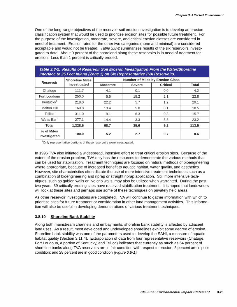
One of the long-range objectives of the reservoir soil erosion investigation is to develop an erosionclassification system that would be used to prioritize erosion sites for possible future treatment. Forthe purpose of the investigation, moderate, severe, and critical erosion classes are considered inneed of treatment. Erosion rates for the other two categories (none and minimal) are consideredacceptable and would not be treated. Table 3.8-2 summarizes results of the six reservoirs investi-gated to date. About 9 percent of the shoreland along these reservoirs is in need of treatment forerosion. Less than 1 percent is critically eroded.
Table 3.8-2. Results of Reservoir Soil Erosion Investigation From the Water/ShorelineInterface to 25 Feet Inland (Zone 1) on Six Representative TVA Reservoirs.
Moderate
4.1
5.5
22.2
13.4
9.1
14.4
68.7
5.2
Critical
0.0
2.1
1.2
0.1
0.3
5.5
9.2
0.7
Total
4.2
22.8
29.1
18.5
15.7
23.2
113.5
8.6
Number of Miles by Erosion ClassSevere
0.1
15.2
5.7
5.0
6.3
3.3
35.6
2.7
Shoreline MilesInvestigatedReservoir
111.7
250.0
218.0
160.8
311.0
277.1
1,328.6
100.0
Chatuge
Fort Loudoun
Kentucky1
Melton Hill
Tellico
Watts Bar1
Total
% of MilesInvestigated
1Only representative portions of these reservoirs were investigated.
In 1996 TVA also initiated a widespread, intensive effort to treat critical erosion sites. Because of theextent of the erosion problem, TVA only has the resources to demonstrate the various methods thatcan be used for stabilization. Treatment techniques are focused on natural methods of bioengineeringwhere appropriate, because of increased benefit to aquatic habitat, water quality, and aesthetics.However, site characteristics often dictate the use of more intensive treatment techniques such as acombination of bioengineering and riprap or straight riprap application. Still more intensive tech-niques, such as gabion walls or live crib walls, may also be utilized when warranted. During the pasttwo years, 39 critically eroding sites have received stabilization treatment. It is hoped that landownerswill look at these sites and perhaps use some of these techniques on privately held areas.
As other reservoir investigations are completed, TVA will continue to gather information with which toprioritize sites for future treatment or consideration in other land management activities. This informa-tion will also be useful in developing demonstrations of various treatment techniques.
3.8.10 Shoreline Bank Stability
Along both mainstream channels and embayments, shoreline bank stability is affected by adjacentland uses. As a result, most developed and undeveloped shorelines exhibit some degree of erosion.Shoreline bank stability was one of the parameters used to develop the SAHI, a measure of aquatichabitat quality (Section 3.11.4). Extrapolation of data from four representative reservoirs (Chatuge,Fort Loudoun, a portion of Kentucky, and Tellico) indicates that currently as much as 64 percent ofshoreline banks along TVA reservoirs are in fair condition with respect to erosion; 8 percent are in poorcondition; and 28 percent are in good condition (Figure 3.8-1).
Chapter 3 Affected Environment
SMI Final Environmental Impact Statement3-26
3.9 Wetlands
3.9.1 Introduction
Wetlands are highly productive and biologically diverse ecosystems that provide multiple publicbenefits such as flood control, reservoir shoreline stabilization, improved water quality, and habitat forfish and wildlife resources.
As defined in TVA Environmental Review Procedures,
Wetlands are those areas inundated by surface or ground water with a frequency sufficientto support, and under normal circumstances, do or would support a prevalence of vegeta-tion or aquatic life that requires saturated or seasonably saturated soil conditions for growthand reproduction. Wetlands generally include swamps, marshes, bogs, and similar areassuch as sloughs, potholes, wet meadows, mud flats, and natural ponds (TVA, 1983).
Along reservoir shorelines, wetlands are transitional ecosystems between terrestrial and aquaticcommunities. The creation of the TVA reservoir system resulted in the loss of thousands of acres ofnatural wetlands throughout the Tennessee River Valley. However, reservoir creation and manage-ment resulted in the formation of many new wetlands areas (Amundsen, 1994).
Although numerous definitions exist for what constitutes a wetland, they primarily include threeidentifying characteristics: hydrophytic vegetation, hydric soils, and wetlands hydrology (NationalResearch Council, 1995).
• Hydrophytic vegetation is defined as plant life growing in water or on a substrate that is at leastperiodically deficient in oxygen as a result of excessive water content.
• Hydric soil is defined as a soil that is saturated, flooded, or ponded long enough during thegrowing season to develop anaerobic (oxygen deficient) conditions in the upper part.
• Wetlands hydrology is generally defined as permanent or periodic inundation or prolonged soilsaturation sufficient to create anaerobic conditions in the soil.
75.9
45.7
Figure 3.8-1. Current Conditions of Shoreline Bank Stability for TVA Reservoirs.
Poor-8%
Fair-64%
Good-28%
Average Bank Stability Score = 3.42
Chapter 3 Affected Environment
SMI Final Environmental Impact Statement 3-27
3.9.2 Wetlands Mapping and Interpretation
The USF&WS National Wetlands Inventory (NWI) is the only comprehensive federal wetlands map-ping effort and is based on the classification system of Cowardin et al. (1979). TVA cooperated withthe USF&WS in the production of several NWI maps for the Tennessee Valley region in the early1980s. TVA continues to use NWI-published standards for cartography, photointerpretation, anddigitization following the Cowardin classification system for reservoir lands planning and other re-source management activities. Much of the information contained in these maps and reports, suchas vegetation structure, hydrologic regime, water quality, and substrate type, is relevant in assessingthe functions of wetlands. Efforts are being made to determine ways to maximize use of NWI mapinformation in assessing wetlands functions (Smith, 1993). Bingham and Roberts (1994) found a highdegree of correspondence between areas mapped as wetlands by NWI and areas that were actuallydetermined to be wetlands by on-site data collection.
TVA uses NWI maps as first-level information for wetlands delineation and assessment to ensureconsistency with provisions of Executive Order 11990 (Protection of Wetlands) and implementation ofNEPA. Due to a lack of quantified information on reservoir shoreline wetlands functions, a qualitativeassessment of impacts to wetlands wildlife and waterfowl use of available wetlands habitats wasconducted. The fact that most knowledge concerning the ecological integrity function is qualitative isnot unique to wetlands (Smith, 1993). Through the public involvement process, state and federalnatural resource management agencies and the general public have expressed the value of TVAreservoir wetlands as wildlife and waterfowl habitats.
3.9.3 Wetlands Analysis Zones and Acreage Calculations
GIS analysis of NWI maps and digital data was conducted for all or portions of six representative TVAreservoirs to determine acreage of wetlands types. NWI maps used in the analysis werephotointerpreted from 1:24,000 and 1:58,000 scale color infrared and true color photography. Thedates of the photography ranged from 1980 to 1992.
Wetland acreages were stratified by the following zones (Figure 3.9-1):
• Zone 1 — area from winter pool to normal summer pool elevation.• Zone 2 — area from normal summer pool elevation to maximum shoreline contour.• Zone 3 — area from maximum shoreline contour to one-fourth mile inland.
Table 3.9-1 lists the acreage of the most common wetlands types found within these zones onselected TVA reservoirs. In Zone 1, 79 percent of all wetlands were the aquatic bed type. In Zones 2and 3, forested wetlands was the dominant type, comprising 82 percent and 89 percent, respectively,of all wetlands within these zones. Wetlands types and wetlands wildlife/waterfowl species that usethese habitats are described in detail in Appendix L.
3.9.4 Wetlands Functions and V alues
Recent wetlands regulatory and protection strategies at both state and federal levels emphasize theneed to assess wetlands functions and values in an effort to protect important public interests.
• Smith (1993) described wetlands functions as the processes necessary for the self-maintenanceof an ecosystem.
• Kusler (1983) listed the primary functions of wetlands as flood conveyance, flood storage, barriersto waves and erosion, sediment and pollution control, habitat for waterfowl and other wildlife, andhabitat for endangered and threatened species.
• Principal functions of TVA reservoir-based wetlands include sediment and pollution control,habitat for waterfowl and other wildlife, and habitat for rare and endangered species.
• Wetlands values are the realized public benefits that result from wetlands functions (Smith, 1993).
Chapter 3 Affected Environment
SMI Final Environmental Impact Statement3-28
• Recognized wetlands values include recreation, water supply and quality, food and timber pro-duction, education and research, and open space and aesthetics (Kusler, 1983).
• Primary values associated with TVA reservoir wetlands include recreation (hunting, fishing,wildlife observation), water quality, and open space and aesthetic values.
3.9.5 Wetlands T rends
There is little quantified information describing wetlands trends for TVA reservoirs and shorelines. Al-though wetlands have been mapped and digitized using a GIS for most of TVA mainstream reservoirs,these data have not been quantified by wetlands types and areas. NWI mapping is available for all TVAreservoirs, but most of the data on tributary and select mainstream reservoirs is not currently available indigital format. In addition, NWI data spans a 15-year time frame, making trend analysis difficult.
1001Chatuge, Chickamauga, lower third of Kentucky, Tellico, Watts Bar, and Wheeler.
Table 3.9-1. Acreage of Wetlands Types Found on Six TVA Reservoirs 1 by ZonesBased on the Cowardin Classification System (1979).
Figure 3.9-1. GIS Wetlands Analysis Zones of a Representative Reservoir.
Zone 2 - Normal summer pool elevationto Maximum Shoreline Contour (MSC)
Zone 1 - Winter pool elevation tonormal summer pool elevation
Water
Zone 3 - MSC to 1/4 mile from MSC
Chapter 3 Affected Environment
SMI Final Environmental Impact Statement 3-29
The area of emergent, scrub-shrub, and forested wetlands on and immediately adjacent to TVAreservoirs has probably remained relatively stable, compared to the trend for these wetlands types inthe Southeast (Hefner et al., 1994). Forested wetlands have been the most heavily impacted onprivate land throughout the TVA region over the last 50 years.
The presence of wetlands on or adjacent to TVA reservoirs appears related to the development statusof the shoreline. Within the one-fourth-mile shoreline area (Zones 1, 2, and 3), the proportion of totalwetlands acreage was greater along undeveloped shorelines than along developed shorelines(Table 3.9-2). This is partially explained by the fact that many wetlands occur in low-lying or flood-prone areas where development is often restricted.
Shoreline Development StatusAttribute
Wetlands Acres
Acres per Mile
Developed
799
1.5
Undeveloped
30,038
9.9
Table 3.9-3. Number and Proportion of Wetlands Acres1 Within One-Fourth-Mile ShorelineArea Surrounding Six TVA Reservoirs2 in Relation to Shoreline Development Status.
Developed
Undeveloped
Totals
1
99
100
3
97
100
244
7,880
8,124
147
17,841
17,988
Zone 1 Zone 2 Zone 3
Acres PercentPercentAcres Acres Percent
ShorelineDevelopment Status
408
4,317
4,725
9
91
100
Table 3.9-2. Wetlands Acreage on Six TVA Reservoirs1 by Zones Along Developed andUndeveloped Shorelines.
1Chatuge, Chickamauga, lower third of Kentucky, Tellico, Watts Bar, and Wheeler (Zone 1 for Wheeler includes onlyaquatic bed wetlands).
Wetlands are not randomly distributed along TVA reservoirs, as substantiated by the acres perdeveloped and undeveloped shoreline mile (Table 3.9-3). Wetlands acreage per undeveloped shore-line mile was over six times greater than along developed shorelines.
3.10 Floodplains/Flood Control
As stated in the TVA Act, one of the primary reasons that TVA was established in 1933 was to “controlthe destructive floodwater in the Tennessee River and the Mississippi River Basins” (U.S. Congress,1933). A series of dams and reservoirs was constructed to make flood control a reality. The opera-tion of the dams and reservoirs provides substantial protection against flooding in the TennesseeValley and in the Ohio and Mississippi River basins.
A common misconception about dams is that they prevent flooding. Floods cannot be prevented, butthe operation of the TVA reservoir system can reduce damages. Efforts are made to reduce the peakflood elevations that would occur naturally without the dams. This is done by holding back waterupstream in the storage tributary reservoirs until the rains have subsided, and then gradually releas-ing water until normal reservoir operations can be resumed. These actions substantially reduce thepeak water elevations that would occur without the reservoir system.
1Determined from GIS analysis of NWI map polygons with a minimum mapping unit size of approximately half an acre.2Chatuge, Chickamauga, lower third of Kentucky, Tellico, Watts Bar, and Wheeler.
Chapter 3 Affected Environment
SMI Final Environmental Impact Statement3-30
Even with the system of dams, there is a floodplain adjacent to the reservoir. The 100-year floodplainis defined as that area inundated by the 100-year flood. The 100-year flood is the level of floodingthat has a 1 percent chance of being equaled or exceeded in any given year and does not indicate atime period of 100 years between floods of this magnitude. Floodplain areas along reservoir shore-lines are normally owned by TVA or covered by TVA flowage easements (Section 1.4.5).
Floodplains provide and support many natural resources and functions of considerable economic,social, and environmental value. These values and benefits include natural wetlands and wildlifehabitat, improved water quality, stormwater management, recreational opportunities, and aesthetics.
3.11 Aquatic Habitat
3.11.1 Introduction
Reservoir construction has greatly impacted the character of the Tennessee River. Theseimpoundments were developed for flood control, navigation, and power generation. However,recreation has become an important benefit of the reservoir system, with sport fishing being one ofthe major attractions.
About 50 to 75 percent of the nutrients and organic materials that flow into a reservoir settle into thesediment and become trapped. This contributes to a higher reservoir productivity than would bepresent in an unimpounded river (Yeager, 1993). Higher productivity, while not desirable from a waterquality standpoint, does enhance the quality of the fishery as long as plant growth does not increaseto eutrophic levels (Section 3.12.2). Tailwater areas, in contrast, are deprived of nutrients and organicmaterial, making them less productive than before the dam was built.
While impoundment has benefited aquatic resources, there have also been negative effects. Prior toimpoundment, low dissolved oxygen (DO) levels (i.e., less than 4 mg/l) were relatively rare occur-rences caused mainly by pollution. Stratification occurs in moderately deep lakes (i.e., more than 16feet) where water takes months to pass through the reservoir. After stratification begins duringsummer, DO levels in the lowermost, cold layer of the reservoir are progressively reduced to 0, due todecomposition of organic materials which have settled to the bottom. This condition seriously impactscommunities of organisms (such as benthic invertebrates) that do not have the mobility to leaveaffected areas. The shallow-water reservoir shoreline area generally is not impacted by stratification.
3.11.2 Benthic Macroinvertebrates
Benthic organisms (e.g., aquatic insects, mussels, crayfish) are a vital part of the food chain ofaquatic systems. These organisms transform nutrients and organic materials into food for fish andother vertebrate predators. Most benthic organisms have specific habitat requirements which dependupon certain physical, chemical, and biological factors. Alterations of any of these factors can causechanges in composition and productivity of benthic communities. Many benthic organisms havenarrow habitat requirements which are often not met in reservoirs.
Benthic communities are extremely limited in the deep portions of tributary and some mainstreamreservoirs, due to the lack of DO during summer stratification; and in the shallow areas of tributaryreservoirs, due to winter drawdowns that leave these areas dry for extended periods. Low DO,excessive current, and cold water temperatures also limit benthic communities in tailwater areasimmediately below the dam in reservoirs with a deepwater release.
Mussels
Freshwater mussels are unusual benthic invertebrates because they are extremely long-lived, havecomplex life cycles (including a time as parasites on fish), and are commercially valuable. Many ofthese mussels live more than 25 years, and the beads made from some shells are used in producingcultured pearls. Nearly all native mussel species occur in stable gravel or cobble substrates which arekept silt-free by flowing water.
Chapter 3 Affected Environment
SMI Final Environmental Impact Statement 3-31
Native mussels are extremely rare in tributary reservoirs for the same reasons mentioned for otherbenthic macroinvertebrates. In mainstream reservoirs, the mussel distribution pattern is more com-plex. Mussels rarely exist in the deepest parts of mainstream reservoirs, probably because thoseareas are covered with soft sediment and may occasionally have very low DO levels. Shallow areasin these reservoirs may contain large populations of a few mussel species if there is enough watermovement to bring in food materials and remove excess silt. The most species-rich mussel communi-ties in mainstream reservoirs occur in the original river channel where bottom conditions and currentsare much the same as they were before the dams were built.
Because of their long lives, sedentary nature, and clumped distribution in areas of suitable habitat,freshwater mussels are highly vulnerable to habitat disruptions or changes in environmental condi-tions. During the last 60 years, native mussel resources have decreased because of habitat lossesand intense harvest pressures. To help counter these losses, state fish and wildlife agencies haveestablished mussel sanctuaries in various parts of the Tennessee River system. Some of thesesanctuaries could be affected by shoreline management activities (Table 3.11-1).
Sanctuary (or Management Area) Boundaries
From Little Chain navigation light upstream to Kentucky Dam
State
KY
TN
TN
TN
TN
TN
TN
AL
AL
AL
Tennessee River Miles
17.8-22.4
103.5-107.8
140.0-141.5
201.9-206.7
416.5-424.7
465.9-471.0
520.0-529.9
253.2-259.4
333.4-336.5
347.2-349.0
East overbank from Tennessee National Refuge upstreamto Rockport Island navigation light
Mouth of Elkin Branch upstream to mouth of Cedar Creek
Tennessee Gas pipeline upstream to Pickwick Landing Dam
Alabama state line upstream to Nickajack Dam
Marine Way upper navigation light upstream to Chickamauga Dam
Hunter navigation light upstream to Watts Bar Dam
Upper end of Seven Mile Island upstream to Wilson Dam
Whitesburg Bridge upstream to head of Hobbs Island
There are 205 species of fish inhabiting the Tennessee River system (Etnier and Starnes, 1993). Thedynamics of fish communities shifted, as a result of reservoir construction. Prior to impoundment, fishcommunities in the Tennessee River were dominated by species which favored riverine conditionswith associated periodic flood events. For the most part, reservoirs stabilized the habitat, reduced theflow of water in most sections, and trapped organic material, which increased nutrient availability.Fish species — such as largemouth bass, bluegill, and crappie — that prefer the more stable environ-ments became much more numerous. Fish species — such as lake sturgeon, most sucker species,sauger, walleye, paddlefish, and other stream-spawning species (i.e., darters and many minnows) —that depend more on current and shoal areas were significantly reduced in numbers and diversity.
Commercial and sport fishing attract people from across the nation to TVA reservoirs. Over 3.5million pounds of commercial fish were harvested during 1993 from TVA reservoirs located in thestate of Tennessee (Todd, 1994). The majority of the catch were catfish, buffalo fish, paddlefish, andfreshwater drum. Recreational fishing accounted for 872,476 trips and 4,362,378 hours of use on 13TVA reservoirs in Tennessee during 1993 (O’Bara, 1994). Extrapolation of these results suggests thatover 2 million trips per year and 10.5 million hours were spent fishing on all TVA reservoirs during1993. Most sought-after species were black bass (48 percent of the total effort) and crappie(15 percent).
Chapter 3 Affected Environment
SMI Final Environmental Impact Statement3-32
Fishing enthusiasts and state fish and wildlife agencies responsible for fisheries management want tomaximize fisheries in the Tennessee Valley. TVA attempts to enhance spawning along the shoreline;once water temperatures at a depth of 5 feet reach 62oF, TVA keeps reservoir pool levels stable for atwo-week period during spring. This is the anticipated peak spawning season for shoreline speciessuch as black bass and crappie. The most productive region of a reservoir for the most sought-afterspecies (black bass and crappie) is along the shoreline because of the spawning requirements ofthese species; the importance of cover such as submerged vegetation; and availability of aquaticinvertebrates as a food source.
Commercial species that require suitable habitat in shoreline areas include catfish — which spawn incavities such as those found in hollow logs or created by groupings of large rocks — and buffalo fish— which broadcast their adhesive eggs over the river bottom or on vegetation. Many nonsport fishspecies also rely heavily on this productive zone of the reservoir. Minnows such as bluntnose andbullhead; shiners such as golden, spotfin, steelcolor, and emerald; brook silversides; and logperch allrequire relatively unspoiled shoreline habitat.
Shoreline development results in modification of adjacent fish and benthic invertebrate habitat andother environmental factors which shape the quality of the fish community. For example, removal ofvegetation in and near the water subjects the area to more nonpoint source pollution from runoff onnearby lands and destroys aquatic habitat. Mining, timber harvesting, domestic and industrial efflu-ents, erosion, agricultural practices, and urbanization have affected nearly all fish habitat in theTennessee River watershed.
3.11.4 SAHI and Existing Conditions
The SAHI described in Appendix G was developed to determine the quality of aquatic habitat adjacentto the shoreline. The index is based upon shoreline habitat characteristics important to maintenanceof good populations of sport fishes (a major concern during public meetings). Data on the followingparameters (which also apply to nonsport fishes) were collected and used to calculate the indexvalues:
• Cover, which in the form of boulders, rootwads, brushpiles, logs, aquatic vegetation, etc., providesshelter for young fish and ambush areas for adult predators.
• Gravel substrate, which is critical for nest-building spawners such as bass and sunfish species.
• Bank stability, which is a measure of erosion that covers spawning areas with silt, limiting spawningsuccess.
• Canopy over shoreline areas, which provides shade as a form of cover, in addition to reducingundesirable overwarming of shallow water during summer.
• Width of riparian zone, which reduces siltation and pollution entering the water.
• Habitat diversity, or number of different habitat types, which increases the number of speciessupported within a reservoir as represented habitats increase.
• Dredging, which removes spawning habitat but can be, at low levels, beneficial in providingaccess routes for adults to shallow spawning areas.
Observed conditions were compared with those anticipated under ideal conditions and a correspondingvalue assigned: good = 5, fair = 3, poor = 1. The scores for each parameter were summed to obtainthe SAHI value. The potential range of SAHI scores (7 - 35) was subdivided into thirds to provide ageneral descriptor of habitat quality (good, fair, poor); however, there is little difference between sitesthat have similar scores.
Chapter 3 Affected Environment
SMI Final Environmental Impact Statement 3-33
Existing Conditions
SAHI results from four representative reservoirs (Chatuge, Fort Loudoun, Tellico, and the lower thirdof Kentucky) were used to describe existing shoreline aquatic habitat conditions with respect toadjacent land uses. Results from these sample reservoirs were expanded to represent shorelineareas and existing land uses around all TVA reservoirs. The estimated average SAHI score for allTVA reservoirs is 24.3 and was used as the baseline for comparing the effects of the alternatives onaquatic habitat (Section 4.9). Sixty percent of the TVA reservoir shoreline aquatic habitat scored fair,7 percent scored poor, and 33 percent scored good (Figure 3.11-1).
Figure 3.11-1. SAHI Results Extrapolated for All TVA Reservoirs.
Fair-60%
Average SAHI Score = 24.3
Good-33%
Poor-7%Existing Conditions
3.12 Water Quality
3.12.1 Introduction
About two-thirds of the approximately 2,100 miles of rivers and large streams in the Tennessee RiverValley are reservoirs impounded by dams (TVA, 1990b). TVA reservoirs support numerous waterquality-dependent human uses, as well as a diversity of fish, freshwater mussels, and other aquaticorganisms. Water bodies within the Tennessee River Valley are classified for specific uses by thestates, and water quality criteria are established for those uses. The water quality of TVA reservoirstypically meets environmental requirements for supporting these varied beneficial uses. With somelocal exceptions, reservoirs within the Tennessee River Valley are generally clean, and water quality isconsidered fair to good (TVA, 1990b, 1995a).
Reservoir Uses
Multipurpose reservoir uses include:
• Recreation, such as swimming, wading, fishing, and boating.• Drinking water supplies.• Industrial water supplies.• Propagation and growth of aquatic life and water-dependent wildlife.• Flood protection.
People use reservoir embayments (i.e., sloughs, coves, sheltered areas off the mainstream) morethan other areas. Residential shoreline development tends to be located along embayment shore-lines which are also preferred sites for marinas. Swimming, wading, fishing, and boating are moreconcentrated in these areas. However, water moves out of embayments more slowly than in the mainreservoir channels. This means that sediment and other pollutants are flushed out of embaymentsmore slowly. As a result, embayments are more environmentally sensitive, and most water qualityproblems, except those related to low DO, are found there. In contrast, the water quality along mainchannel shorelines is usually better because:
• Water flows more quickly,• Wave action is greater and mixes the water,• Water volume is greater, and• Fewer people use main channel areas.
Factors Affecting W ater Quality
Several factors currently determine whether reservoirs and embayments meet water quality criteriafor established uses. Reservoir construction along the Tennessee River profoundly affected thequantity and quality of water passing through the system. Naturally-occurring seasonal stratification(Section 3.11.1) affects water quality in both the lower layers of reservoirs and the stream reachesinto which the reservoirs discharge. Seasonally low levels of DO are the primary problem. Withimplementation of the Lake Improvement Plan (TVA, 1990b), many miles of habitat historicallyaffected by low DO and lack of minimum flows have been recovered within tributary and selectedmainstream reservoirs, as well as below their dams.
Although water quality of TVA reservoirs is generally good, the public, as well as state and federalresource and regulatory agencies, have identified other concerns. Many of the remaining pollutionproblems are related to diverse, nonpoint sources of pollution resulting from watershed developmentand improper land use practices both in the tributary watersheds and along reservoir shorelines.These problems include (1) nutrient enrichment causing occasional nuisance growth of aquaticplants, including algae, and (2) bacterial contamination. TVA's Lake Improvement Plan (TVA, 1990b)also recognizes and acknowledges the importance of additional nonpoint sources contributing tonutrient and water quality problems.
3.12.2 Nutrient Enrichment
Phosphorus and nitrogen are the most important added nutrients that affect water quality. These andother nutrients come from several major nonpoint sources, including:
• Industrial/commercial processes,• Municipal sewage,• Agricultural areas and urban development both along reservoirs and in watersheds draining into
the river system, and• Soils.
Industrial/Commercial Processes . Various point-source industrial processes produce and dischargenutrients containing nitrogen and phosphorus into water bodies. In some instances, additional runoff fromindustrial sites storing raw materials or finished products contributes nutrients to reservoirs and streams.
Chapter 3 Affected Environment
SMI Final Environmental Impact Statement 3-35
In the Tennessee River Valley, pesticide, herbicide, and industrial chemical pollution potentiallyentering the human food chain is localized and predominantly limited to five industrial/commercialchemicals (PCBs, chlordane, DDT, dioxins, and mercury). Three of these are no longer commerciallyavailable in the United States. These chemicals do not dissolve well in water, so they are foundmostly in mud on the bottom of rivers and lakes. However, they can build up in the fatty tissues offish, particularly those that feed on the lake bottom. TVA cooperates with state agencies checking fortoxic contamination of fish tissue. The states then decide whether to issue advisories on fish con-sumption for a particular area. Chlordane has been associated with fish consumption advisories inTennessee. Whether the source is lawn runoff or improper chemical use and disposal is unknown.No other potential sources of chemically laden runoff from insect or weed killers have been associ-ated with any fish consumption advisories.
Municipal Sewage . Some reservoir water quality impacts from residential shoreline developmentcurrently come from nutrients contributed by failing septic systems and inadequate package sewagesystems, as well as the additional contributions from municipal sewage systems. Even the bestdesigned and operated secondary sewage treatment facilities do not remove substantial amounts ofnitrogen and remove only modest percentages of phosphorus.
Information on the number and extent of leaking and failed septic systems along TVA reservoirs isscarce. Many lakefront homes are not connected to municipal wastewater treatment systems and relyon septic tanks and field lines for treatment. A study conducted by Swanson Environmental, Inc.,(TVA, 1985a) indicates that septic systems were failing and contributing elevated nutrient levels toembayments on Guntersville Reservoir. Accelerated lake eutrophication in other areas of NorthAmerica has also been linked to malfunctioning domestic sewage systems releasing bacteria andnutrients into lake water and bottom sediments. The cumulative addition of nutrients from existingdevelopment comes from both properly operating and failing septic systems; package sewage sys-tems operated for specific subdivisions; and municipal wastewater treatment systems. The amount ofnutrients added is related to the total number of septic systems, the population density, and theproximity of development to the shoreline.
Agricultural Areas and Urban Development . Soil characteristics in certain areas of the TennesseeRiver Valley, abundant rainfall, and the economic encouragement to adopt row-crop-practice systemscontribute to erosion of agricultural areas near reservoirs and tributary streams. Construction activi-ties related to residential or other urban development also mobilize soils. In addition to siltationproblems, erosion of agricultural lands moves various agricultural chemicals, including fertilizers, intostreams, rivers, and reservoirs. Removal of vegetation in the shoreline management (riparian) zone isthe major obstacle in protecting water quality. Improper management of shoreline vegetation reducesits capacity to stabilize banks and filter lawn fertilizers (nutrients) and chemicals (pesticides andherbicides).
Nutrients Naturally Occurring in Soils . Soils of the Valley also contain naturally occurring nutrientswhich are mobilized and carried into water bodies as a result of certain agricultural and soil-disturbingactivities. These nutrients also affect the productivity of reservoirs, rivers, and streams.
Algal and Aquatic Plant Growth Problems
Once nutrients enter a water body, the main effects are associated with a process called eutrophication.Eutrophication in TVA tributary reservoirs leads to increased productivity of algae. In mainstreamreservoirs, eutrophication typically results in abundant production of aquatic plants and in floatingalgal mats along shorelines or embayments. Undesirable algal and aquatic plant growth are respon-sible for much of the water quality deterioration that accompanies eutrophication. Excessive produc-tion often results in increased demand for management and control of aquatic plant growth.
There are no uniform guidelines for what constitutes excessive productivity of algae or aquaticplants. For instance, high algal or aquatic plant production is desirable for maximum fish productionbut undesirable for protecting community water supplies or maintaining access to marinas and
Chapter 3 Affected Environment
SMI Final Environmental Impact Statement3-36
residentially developed shorelines. Impacts on water quality from excessive algal productivity oroverproduction of particular algal types (e.g., bluegreens or diatoms) in TVA reservoirs have included:
• Taste and odor problems in water supplies.
• Odor incidents in embayments.
• Filter clogging and increased treatment costs at industrial water treatment plants.
• Discoloration and oily surface films.
• Surface algal blooms and scums.
• Algal mats in embayments.
• Contribution to DO depletion due to decomposition of algae and plants.
Greater depletion of oxygen increases the costs of operation and maintenance of aerating technologiesand affects TVA’s ability to meet DO targets established in the Lake Improvement Plan (TVA, 1990b)for reservoir releases.
After finding all existing methods of assessing eutrophication to be inappropriate for application,Placke (1983) developed a system of evaluating eutrophication specific to TVA reservoirs. Reservoirswere ranked from least to most eutrophic. The ranking of tributary reservoirs was: Hiwassee, BlueRidge, Chatuge, Norris, Fontana, Watauga, South Holston, Tims Ford, Cherokee, Douglas, andBoone. The ranking of mainstream reservoirs was: Pickwick, Kentucky, Chickamauga, Nickajack,Wilson, Fort Loudoun, Watts Bar, Wheeler, and Guntersville.
Current Nutrient Levels
Estimated average nutrient (total phosphorus) amounts added to embayments and total waterflowfrom existing residential shoreline development are shown in Figure 3.12-1 for eight representativeTVA tributary and mainstream reservoirs. Nutrient concentrations added by residential shoreline
Figure 3.12-1. Average Amounts and Rang e of Nutrient Phosphorus (T otal P) Fr om CurrentResidential Shoreline De velopment on Eight Representative TVA Reser voir s1 Contrib uted atthe Emba yment Le vel or Reser voir -Wide .
1Blue Ridge, Chatuge, Cherokee, Chickamauga, Fort Loudoun, Nickajack, Tims Ford, and Wilson.
Chapter 3 Affected Environment
SMI Final Environmental Impact Statement 3-37
development currently do not exceed levels likely to produce changes in aquatic communities orindependently affect suitability of water bodies for human uses. However, these amounts of additionalphosphorus do substantially increase the total nutrients available in a reservoir and are probablyhaving some effect on the productivity of aquatic communities in highly developed embayments.
3.12.3 Bacterial Contamination
Fecal coliform contamination can directly affect the acceptability of areas for water contact recreationsuch as swimming, wading, and fishing. The presence of fecal coliform bacteria indicates that waterhas been contaminated by human or animal wastes, which may contain disease-causing microorgan-isms. No reservoir, lake, or stream is completely free of pathogenic organisms, but the lower the fecalcoliform count, the less chance there is of persons becoming ill from water contact.
Urban runoff and inadequate municipal wastewater treatment are frequent causes of high bacteriaconcentrations in reservoirs. Large waterfowl populations raise fecal coliform concentrations in a fewareas. For instance, the Forest Service temporarily closed one of its swimming areas in 1995 due tohigh bacteria concentrations caused by local geese. Several other sources, including failing septicsystems, livestock operations, and wildlife management areas, contribute to high fecal coliformconcentrations in streams entering reservoirs.
There are only a few reservoir sites which do not meet state criteria for water contact recreation.However, the state of Tennessee has issued public advisories against water contact at 12 sites in TVAreservoir embayments or at the mouths of streams entering TVA reservoirs. Urban runoff is not thesole source for the water contact advisories; however, inefficient wastewater systems and combinedsewer overflows are primary causes. TVA sampled 129 reservoir sites in 1993 and 1994 other thanthose posted by the state of Tennessee advising against water contact (TVA, 1995a). Two of the sitesdid not meet state criteria, and an additional 14 sites failed to meet the criteria when samples weretaken within 48 hours of rainfall. Most of the high concentrations in TVA samples were due to largepopulations of waterfowl, but one of the two sites not meeting state criteria was due to urban runoff.
3.13 Recreational Use of Shoreline
3.13.1 Introduction
The Tennessee Valley region provides diverse scenic and outdoor recreation resources. TVAreservoirs support a wide variety of outdoor recreation activities, including fishing, skiing, hunting,swimming, and camping. Travel and tourism associated with these recreation resources representsignificant and growing contributions to the economy of the region.
3.13.2 Total V isitation
Recreational use of TVA reservoirs has attained high levels. The last year that TVA collectedcomprehensive recreation visitation data was 1978. In that year, an estimated 71 million visitsoccurred on TVA reservoirs and lands, including Land Between The Lakes. Figures 3.13-1, 3.13-2,and 3.13-3 reveal trends in visitation data collected by Tennessee State Parks (Boswell, 1995);USACE Nashville District (Yann, 1995); and Joe Wheeler State Park, Alabama (Thrasher, 1995). Ifsimilar trends were observed on TVA reservoirs, estimated recreation visitation in 1995 would be 113million visits. This estimate encompasses all recreational visits to TVA reservoirs and surroundingdeveloped and undeveloped lands.
3.13.3 Recreation Activities Occurring Along the Shoreline
Fishing from the bank and by boat are the most popular recreation activities that occur along theshoreline. In TVA Land Management and Use Study (Larsen, 1993a), 73 percent of those interviewedsaid they participated in these activities at some time. Forty-one percent of respondents said theyfished from a boat, and 32 percent fished from the bank.
Chapter 3 Affected Environment
SMI Final Environmental Impact Statement3-38
Figure 3.13-1. Visits to 14 Tennessee State Parks on TVA Reservoirs, 1977-1995.N
umbe
r of
Vis
its (
mill
ions
)
78 94939291908988878684 858379 80 81 82 95
Fiscal Year
12
11
10
9
8
7
6
577
Figure 3.13-3. Lodge Guests at Joe Wheeler State Park, 1985-1995.
Num
ber
of G
uest
s (t
hous
ands
)
Fiscal Year
130
110
100
90
80
70
6085
120
86 87 88 89 90 91 92 93 94 95
Figure 3.13-2. Visitation to USACE Projects in the Nashville District, 1976-1994.
Num
ber
of V
isito
rs (
mill
ions
)
77 93929190898887868583 848278 79 80 81 94
Year
55
45
40
35
30
25
2076
50
Chapter 3 Affected Environment
SMI Final Environmental Impact Statement 3-39
Other recreational uses of the shoreline include:
• Picnicking and swimming. People come by boat and by car to shoreline areas that provide waterof reasonable depth for swimming.
• Camping on undeveloped shoreline land.• Walking along the shoreline, especially when the lake bottom is exposed in fall and winter.• Hunting.
The following recreational activities occur when adjacent landowners use existing shoreline facilities,including docks, boathouses, and swim floats:
• Boating.• Swimming, picnicking, fishing, and other active recreational uses of the lake.• Relaxing and observing activities occurring on the lake. This includes general enjoyment of the
lake environment.
According to TVA Lake Users Study (Larsen, 1993b), 59 percent of lake users chose a lake becauseit was closest to them. Fifty-three percent also had used other TVA lakes. When choosing a lake,other responses in order of frequency of occurrence were: best fishing (25 percent), cleanliness(12 percent), recreation facilities (10 percent), and familiarity (9 percent). Together, scenery, setting,and quality of management accounted for 7 percent of the reasons for choosing a lake.
Boat and bank fishing accounted for 33 percent of the respondents’ primary use of TVA lakes,followed by camping in developed campgrounds (16 percent), boating (14 percent), enjoying scenery(10 percent), and swimming and/or sunbathing (8 percent). Other uses included: camping in unde-veloped areas (4 percent), picnicking (4 percent), hiking (4 percent), skiing (2 percent), bikeriding (1 percent), jet skiing (1 percent), photography (1 percent), and other (1 percent).
3.13.4 Informal Recreation
TVA allows the public to use undeveloped lands for informal recreation. For example, most islandsand many shoreline areas accessible by road or boat are frequently used for fishing and primitivecamping. On holiday weekends during the summer, when public and commercial recreation areasare full, people who want to camp on undeveloped lands often cannot find a camping spot.
Undisturbed and undeveloped reservoir shorelines are highly valued for walking, nature observation,bank fishing, and other passive forms of recreation, according to public meetings participants (TVA,1988, 1990a).
When shorelands are developed with residential shoreline alterations and industrial facilities, theirpublic recreational value is lost. In some cases private property owners maintain public land as if itwere a part of their own yard. Thus, the public recreational value is lost because the land appears tobe private, and people no longer feel welcome to stop along these public shorelands to fish, picnic,swim, or camp. Also, some backlying landowners routinely ask visitors to leave the strip of public landfronting their lot. Actions like these give the impression that public lands are no longer available forpublic use.
Baseline of Existing Informal Recreational Opportunities
The effects of the alternatives on informal recreational use of the shoreline are addressed in Section4.11. The baseline for this analysis is the number of existing informal recreational opportunities forday-use activities, camping, and hunting on undeveloped public land.
To establish this baseline, the total number of shoreline miles available for public use was first deter-mined for each of these activities. From this total, the number of shoreline miles with potential forrecreational activity was calculated. Using these estimates, the number of miles suitable for recre-ation was determined (Table 3.13-1). Recreation planning standards were then applied to the numberof suitable shoreline miles, to yield existing recreational opportunities. A more detailed explanation ofeach of these steps is as follows.
Chapter 3 Affected Environment
SMI Final Environmental Impact Statement3-40
Total Available Miles . The total number of shoreline miles available for public use was calculated bysubtracting the number of miles of undeveloped flowage easement shoreline from the total number ofundeveloped shoreline miles. This yielded an estimate of approximately 7,500 shoreline milesavailable for day-use activities (i.e., bank fishing, walking the shoreline, swimming) (Table 3.13-1).This number was reduced somewhat for camping and hunting because various natural resourcemanagement agencies prohibit these activities in some areas.
Potential Miles . Landrights data and land characteristics from six representative reservoirs(Chickamauga, Kentucky, Nickajack, Tellico, Watts Bar, and Wheeler) were used to determine thenumber of shoreline miles with potential for informal recreational activity. Using the total shorelinemiles available (described above) as a basis, shoreland on these six reservoirs was evaluated accord-ing to the following spatial criteria:
• For day-use activities, a tract of land had to be at least 500 feet long and at least 25 feet deepfrom the shoreline to the backlying property line.
• For informal camping, a tract of land had to be at least 500 feet long and at least 100 feet deepfrom the shoreline to the backlying property line.
• For hunting, a tract of land had to be at least 500 feet long, and the backlying property line had tobe 300 feet from the winter drawdown elevation. A 300-foot minimum width from the winterdrawdown elevation was chosen because most hunting takes place in the winter, and this widthprovides the minimum required distance from dwellings for discharge of firearms.
The lengths of shoreline segments meeting these criteria were summed to give shoreline mileshaving potential for day-use, informal camping, and hunting activities. Using these estimates, the ratioof potential miles to available miles was calculated for each of the recreational activities. These ratioswere then multiplied by the number of available miles for each reservoir, resulting in a Valleywideestimate of potential miles (Table 3.13-1).
Suitable Miles . To determine the number of miles suitable for informal recreational activities, slope ofthe shoreline was first calculated at 1-mile intervals for each reservoir. Using the number of potentialmiles (described above) as a basis, steep areas were then eliminated according to the following criteria:
• Day-use activities: Shoreline areas with slopes greater than 30 percent were eliminated.
• Informal camping: Shoreline areas with slopes greater than 40 percent were eliminated.
• Hunting: No shoreline areas were eliminated.
The result was the total number of miles suitable for the three informal recreational activities(Table 3.13-1). At current development levels, only 18 percent of the total undeveloped shorelineavailable for public use is suitable for day-use activities. For informal camping and hunting theseproportions are 14 and 17 percent, respectively.
Existing Informal Recreational Opportunities . State Comprehensive Outdoor Recreation Planningstandards from Tennessee and Kentucky were applied to the number of suitable shoreline miles todetermine existing recreational activity occasions (Table 3.13-2).
Camping (Miles)
7,300
1,500
1,000
Day Use (Miles)
7,500
1,900
1,300
Hunting (Miles)
6,600
1,100
1,100
Informal Recreation Activity
Table 3.13-1. Number of Undeveloped Shoreline Miles Available for Public Use Comparedto Miles With Potential for and Suitable for Informal Recreation by Type of Activity.
Undeveloped Shoreline
Total Available
Potential
Suitable
Chapter 3 Affected Environment
SMI Final Environmental Impact Statement 3-41
3.14 Aesthetic Resources
3.14.1 Introduction
Based on the number of public comments TVA received by SMI participants, it is apparent thataesthetic values are important. In order to determine existing public preferences, both qualitative andquantitative studies were used. These sources include:
• The 1993 Gallup Poll, TVA Land Management and Use Study (Larsen, 1993a).• Public comments generated during scoping.• The 1995 questionnaire, Viewing Tennessee Valley Shoreline (Appendix H).
3.14.2 Findings of the Gallup Poll, TVA Land Management and Use Study , January 1993
This telephone poll surveyed 1,652 lake users who lived in counties which abut TVA reservoirs. Thestudy showed that almost 7 out of 10 respondents rated the beauty of the shoreline as excellent orgood. According to those surveyed, the most important attributes of scenic quality were an abun-dance and variety of trees (37 percent), wildlife (10 percent), and cleanliness (10 percent). Trash andlitter (52 percent), water quality problems (16 percent), fluctuating water levels (7 percent), andcertain types of development (6 percent) were listed as detriments to visual quality.
3.14.3 SMI Public Scoping
The public was asked to comment on the way TVA manages its reservoir shoreline. Approximately7,800 comments were received from over 2,000 participants. Numerous comments stressed theimportance of natural beauty. Wildlife, trees/natural vegetation, and an undeveloped shoreline werelisted as positive visual attributes. Trash/litter and erosion were listed as the main detriments to visualquality. Downed trees and debris also created a negative impression. A considerable number ofcomments supported standards for the design, construction, and maintenance of waterfront facilities.
These studies suggest that aesthetic qualities are determined by at least three main criteria:
• Presence of viewable wildlife, trees, and natural landscape features.• Absence of trash/litter, erosion, and natural debris.• Amount and condition of shoreline development.
3.14.4 Results of the TV A Questionnaire, Viewing T ennessee V alley Shoreline
A questionnaire (Appendix H) was mailed to previous SMI participants to obtain a more comprehensiveunderstanding of visual preferences related to residential shoreline development. This survey re-sulted in 663 responses (a 70 percent return rate).
The vast majority of respondents (96 percent) indicated that the appearance of residential shorelinedevelopment was either “extremely important” (74 percent) or “very important” (22 percent) to theirenjoyment of the reservoir. About 4 percent of the respondents disclosed that the appearance ofresidential shoreline development was not important, or they did not have an opinion.
Number of Annual Opportunities
700,000
580,000
64,000
1,344,000
Activity
Day Use
Informal Camping
Hunting
Total
Table 3.13-2. Estimated Number of Existing Informal Recreational Opportunitiesby Activity.
Chapter 3 Affected Environment
SMI Final Environmental Impact Statement3-42
3.14.5 Existing Conditions
Preference scores of four measurement indicators (Section 1.8.10) were used to gauge the effects ofthe alternatives on the visual quality and scenic beauty of TVA reservoirs. Baseline conditions foraesthetic resources using these indicators are as follows:
Water-Use Facility Design. Current shoreline structures include a variety of land- and water-basedfacilities but generally consist of fixed and floating piers and docks, decks, patios, steps, and boat-houses. These water-use facilities vary in size, shape, color, and building materials.
Density. The distance between private docks varies. Sometimes docks appear crowded, particularlyin coves. In certain situations, neighbors cooperatively construct community slips.
Amount of Residential Shoreline Development. The amount of residential shoreline developmentvaries a great deal between reservoirs (Section 3.4). For example, Boone, Fort Loudoun, and WilsonReservoirs are more than 50 percent developed. Conversely, eight reservoirs (Apalachia, Bear CreekProject, Hiwassee, Kentucky, Normandy, Ocoee, Tellico, and Wheeler) are relatively undeveloped(less than 10 percent). As of 1994, almost 13 percent of the shoreline had been developed forresidential purposes. However, if current trends continue, TVA estimates that the majority of theshoreline could be developed within the next 25 years.
Shoreline V egetation Alterations. Developed shoreline areas are subject to various levels ofvegetation management, ranging from little vegetation clearing to more extensive disturbance ofnative vegetation and introduction of nonnative plant species. In many cases, public shorelines areroutinely mowed and maintained as an extension of adjoining residential lawns.
3.15 Cultural Resources
3.15.1 Introduction
TVA is mandated under the National Historic Preservation Act of 1966 and the ArchaeologicalResources Protection Act of 1979 to protect significant cultural resources (i.e., archaeological re-sources and historic structures) located on TVA lands or affected by TVA actions. Therefore, TVA isresponsible for the protection of literally thousands of cultural resources.
For the past 12,000 years, through changing climates and environmental conditions, the TennesseeRiver Valley has attracted humans because of its system of water routes and its abundance of naturalresources. Areas where Native Americans once dwelled are often the same places where currentgenerations want to live. Just as people do today, prehistoric Native Americans chose living sites thatwere reasonably level, well drained, not prone to flooding, and near water sources. As in the past,one popular area for habitation today is along waterways. However, distributed along these waterroutes are numerous archaeological sites or areas where archaeological resources are found.
3.15.2 Archaeological Resources
An archaeological resource is defined as any material remains of human life or activities which couldprovide scientific or humanistic understandings of past human behavior and cultural adaptation.Archaeological resources could include, but are not limited to, remains of surface or subsurfacestructures, such as domestic, cooking, or ceremonial structures, earthworks, fortifications, cookingpits, refuse pits, and burial pits or graves. Other examples of archaeological resources include wholeor fragmentary tools, weapons, containers, ceramics, human remains, rock carvings or rock paintings,and all portions of shipwrecks (18 CFR Part 1312.3). Archaeological sites that occur along TVAreservoir shorelines include those from the following time periods: Paleo (10,000 BC - 7,500 BC),Archaic (7,500 BC - 1,000 BC), Woodland (1,000 BC - AD 1,000), Mississippian (AD 1,000 - AD1,650) and Historic (AD 1,650 - AD 1,900).
Chapter 3 Affected Environment
SMI Final Environmental Impact Statement 3-43
In response to this federal legislation, TVA conducts inventories of its lands to record significantarchaeological sites. Reservoir land is sampled to get an idea of archaeological site types anddistribution, with 80 percent of the sampling conducted along the shoreline. Sampling also occurs atthe confluence of streams with the main river channel.
Five mainstream reservoirs (Chickamauga, Guntersville, Nickajack, Pickwick, and Wheeler), or about3,370 miles of shoreline, have been systematically surveyed for archaeological resources. Fromthese surveys, 1,722 archaeological sites were identified along the shoreline or in the shoreline area.
Site distribution models developed from these survey data (Solis and Futato, 1987) indicate thatdistribution and density of Native American archaeological sites can vary greatly. Solis and Futato(1987) categorized TVA-controlled lands adjacent to Guntersville Reservoir by soil type, order ofnearest water source, distance to water source, elevation, and topographic relief. They found thatarchaeological sites were most likely to occur on terraces or stream bottoms close to the main riverchannel or its primary tributaries. However, significant site distribution variables may be different inother parts of the Tennessee Valley. Most of these known archaeological sites are currently situatedon undeveloped land (Table 3.15-1).
(Number of Sites)
52
29
2
52
36
171
(Number of Sites)
380
348
24
351
448
1,551
Developed LandUndeveloped Land
Table 3.15-1. Current Number of Archaeological Sites on Undeveloped and DevelopedLand for Five Reservoirs.
Reservoir
Chickamauga
Guntersville
Nickajack
Pickwick
Wheeler
Total
Even though the majority of shoreline has not been surveyed, the total number of archaeological sitescan be extrapolated using the following assumptions:
1. Unsurveyed reservoirs have similar numbers of sites per mile of shoreline.
2. The upper end of most reservoirs has more sites because the floodplain is not inundated.
3. Most sites are located along undeveloped shoreline.
Conservatively estimated, there are at least 5,500 archaeological sites along reservoir shorelines thatcould be affected by shoreline development.
Currently, these archaeological sites are protected by conducting site-by-site surveys of areas whereground-disturbing activities are scheduled to occur. If significant archaeological resources are found,either the ground-disturbing activity is denied or its impacts are mitigated. Ground-disturbing activitiesthat could be harmful to archaeological sites include channel excavation; construction of boat docks,piers, and retaining walls; and vegetation removal.
3.15.3 Historic Structures
A significant historic structure is defined as any building or structure included in, or eligible forinclusion in, the National Register of Historic Places (36 CFR Part 800.2). To be eligible for theNational Register, a structure must generally be at least 50 years old or older and meet a set ofcriteria established by the Secretary of the Interior (refer to 36 CFR Part 60 for further information onNational Register Criteria).
Chapter 3 Affected Environment
SMI Final Environmental Impact Statement3-44
Besides archaeological resources, TVA must protect any significant historic structures located alongthe shoreline, in the shoreline area, or on backlying property. Historic structures are not as prevalentalong the shoreline as archaeological resources. Most of the structures located along the shorelinewere either moved or destroyed when the reservoirs were built. However, the remains of thesestructures, such as foundations of houses or outbuildings, are considered to be archaeologicalresources and are protected under federal law. As noted above, historic structures are rarely locatedalong TVA’s shoreline or in the shoreline area but, rather, are located primarily on backlying privateproperty. Again, these sites are protected by conducting site-by-site surveys of specific project areas.In most cases, any visual disturbance can be decreased with vegetative SMZs or other forms ofmitigation.
3.16 Socioeconomics
3.16.1 Introduction
From comments received during public involvement, TVA has determined that socioeconomics is akey issue in the SMI. Population, income and employment, and property values are the measurementindicators for this issue. Baseline data related to these indicators are presented below.
3.16.2 Population
In 1994 counties which border the reservoirs had a total estimated population of about 3.1 million(Table 3.16-1). About 38 percent of this population was concentrated in five counties with populationsgreater than 100,000 (see Appendix N for population of individual counties in the vicinity of eachreservoir). These counties and their metropolitan areas are Madison (Huntsville) and Morgan(Decatur) in Alabama and Sullivan (Johnson City-Kingsport-Bristol), Knox (Knoxville), and Hamilton(Chattanooga) in Tennessee. Outside of the metropolitan areas, which include these five plus Flo-rence, Alabama, much of the shoreline is highly rural.
From 1980 to 1994, population of the reservoir counties grew by 10.6 percent, well below the nationalgrowth rate of 14.9 percent. However, during the latter part of that period, 1990 to 1994, thesecounties had a growth rate of 5.6 percent, above the national rate of 4.7 percent.
Growth has not been evenly distributed throughout the region. The western commercially navigablegroup of counties is the only group that has grown faster than the average for all reservoir countiessince 1980. However, the fastest-growing counties, those growing more than 20 percent between1980 and 1994, are located around Knoxville, around Huntsville, at Nottely and Chauge Reservoirs innorth Georgia, and at Watts Bar in East Tennessee (Table 3.16-2).
Reservoir Group 2
Eastern Commercially Navigable
Eastern Tributary3
Western Commercially Navigable
Western Tributary3
Total, All Reservoir Counties 4
Population Percent Increase
1980
1,023,638
798,499
867,321
215,311
2,802,150
1990
1,057,859
828,166
929,462
222,209
2,934,114
1994
1,115,380
873,694
985,903
231,532
3,098,559
1980-94
9.0
9.4
13.7
7.5
10.6
1990-94
5.4
5.5
6.1
4.2
5.6
Table 3.16-1. Population of Counties Along TVA Reservoirs, 1980-1994. 1
1Source: U.S. Department of Commerce, Bureau of the Census (1995).2See Classification in Appendix N.3All commercially nonnavigable reservoirs are included in the tributary classifications.4Total is slightly less than the sum of the groups because a few counties are in more than one group.
Chapter 3 Affected Environment
SMI Final Environmental Impact Statement 3-45
Urbanization trends have impacted many reservoir counties over the last several decades. As shownin Figures 3.16-1, 3.16-2, and 3.16-3, population density has increased greatly in some areas, inparticular North Alabama and the eastern Valley. In 1930 only one reservoir county, Knox County,Tennessee, had a population density greater than 300 persons per square mile. By 1994 four morecounties had passed this level: Madison County, Alabama; and Hamilton, Hamblen, and SullivanCounties, Tennessee. Near these five counties were several others where the density level hadincreased to over 100 persons per square mile.
Current Shoreline Population
Population data are not available for the area along the shoreline. However, a rough estimate of thecurrent shoreline population can be made. The sample of reservoir subdivisions (Section 3.4.5)averages 20.8 developed lakefront lots per shoreline mile. Assuming that this average applies to alldeveloped residential shoreline (1,383 miles), there are about 28,800 developed lakefront lots. Ac-cording to the Gallup poll (Larsen, 1993b), approximately 80 percent, or about 23,000 lots, are beingused as full-time residences. Assuming these households are the national average size of 2.67persons (U.S. Department of Commerce, 1995), there are about 61,000 people now living on lake-front properties.
Current Backlot Population
The subdivision data also show that, on average, a subdivision has 1.1 backlots for each lakefront lot.Assuming that 90 percent of these backlots are used as full-time residences and also have anaverage household size of 2.67, there are an additional 76,000 persons in these developments.
Current T otal Population
There are an estimated 137,000 people living on the lakefront or in backlots associated with lakefrontdevelopments. This represents about 1.6 percent of the 1994 population of the Tennessee Valley201-county region (8.7 million).
44.9
40.5
31.0
30.4
26.3
24.8
22.9
21.6
20.3
1994
13,606
58,184
258,035
7,350
58,099
14,607
35,078
94,565
8,942
Population1980
9,390
41,418
196,966
5,638
46,005
11,707
28,553
77,770
7,431
County
Union
Sevier
Madison
Towns
Limestone
Union
State
GA
TN
AL
GA
AL
TN
Tellico, Watts Bar
Fort Loudoun, Tellico
Chickamauga, Watts Bar
TN
TN
TN
Loudon
Blount
Meigs
PercentIncrease
1Source: U.S. Department of Commerce, Bureau of the Census (1995).
Table 3.16-2. Fastest Growing Counties (More Than 20 Percent) Along TVA Reservoirs,1980-1994.1
Reservoir
Nottely
Douglas
Wheeler
Chatuge
Wheeler
Norris
Ft Loudoun, Melton Hill,
Chapter 3 Affected Environment
SMI Final Environmental Impact Statement3-46
Fig
ure
3.16
-1.
Pop
ulat
ion
Den
sitie
s of
Ten
ness
ee V
alle
y C
ount
ies
Bor
derin
g T
VA R
eser
voirs
, 193
0.
Kno
xvill
e
Cha
ttano
oga
Birm
ingh
am
Atla
nta
Nas
hvill
e
KY
TN
NC
GA
AL
MS
ILV
A
SC < 50
50 -
100
100
- 300
> 30
0
Per
sons
per
Squ
are
Mile
N20
Mile
s
20K
ilom
eter
s
40
6040
100 0
10
WA
SH
ING
TON
JOH
NS
ON
SU
LLIV
AN
WA
SH
ING
TON
CA
RT
ER
CO
CK
E
SE
VIE
R
SW
AIN
BLO
UN
T
GR
AH
AM
CH
ER
OK
EE
CLA
YP
OLK
MC
MIN
N
UN
ION
BR
AD
LEY
MA
RS
HA
LL
JAC
KS
ON
FR
AN
KLI
NM
AR
ION
BE
DF
OR
D
CO
FF
EE
MO
OR
E
RH
EA
LOU
DO
N
KN
OX
UN
ION
JEF
FE
RS
ONHA
MB
LEN
GR
AIN
GE
R
CLA
IBO
RN
EH
AW
KIN
SC
AM
PB
ELL
MA
DIS
ON
LIM
ES
TON
E
LAW
RE
NC
E
MO
RG
AN
WIN
STO
NM
AR
ION
FR
AN
KLI
N
CO
LBE
RT
LAU
DE
RD
ALE
WAY
NE
HA
RD
IN
DE
CAT
UR
PE
RR
Y
HU
MP
HR
EY
SB
EN
TON
HE
NR
Y
ST
EW
AR
T
TR
IGG
CA
LLO
WAY
MA
RS
HA
LL
LYO
N
LIV
ING
STO
N
MO
NR
OE
FAN
NIN
HE
ND
ER
SO
N
HO
US
TON
TIS
HO
MIN
GO
HA
MIL
TON
RO
AN
E
ME
IGS
AN
DE
RS
ON
TOW
NS
Chapter 3 Affected Environment
SMI Final Environmental Impact Statement 3-47
Fig
ure
3.16
-2.
Pop
ulat
ion
Den
sitie
s of
Ten
ness
ee V
alle
y C
ount
ies
Bor
derin
g T
VA R
eser
voirs
, 196
0.
Kno
xvill
e
Cha
ttano
oga
Birm
ingh
am
Atla
nta
Nas
hvill
e
KY
TN
NC
GA
AL
MS
ILV
A
SC < 50
50 -
100
100
- 300
> 30
0
Per
sons
per
Squ
are
Mile
N20
Mile
s
20K
ilom
eter
s
40
6040
100 0
10
WA
SH
ING
TON
JOH
NS
ON
SU
LLIV
AN
WA
SH
ING
TON
CA
RT
ER
CO
CK
E
SE
VIE
R
SW
AIN
BLO
UN
T
GR
AH
AM
CH
ER
OK
EE
CLA
YP
OLK
MC
MIN
N
UN
ION
BR
AD
LEY
MA
RS
HA
LL
JAC
KS
ON
FR
AN
KLI
NM
AR
ION
BE
DF
OR
D
CO
FF
EE
MO
OR
E
RH
EA
LOU
DO
N
KN
OX
UN
ION
JEF
FE
RS
ONHA
MB
LEN
GR
AIN
GE
R
CLA
IBO
RN
EH
AW
KIN
SC
AM
PB
ELL
MA
DIS
ON
LIM
ES
TON
E
LAW
RE
NC
E
MO
RG
AN
WIN
STO
NM
AR
ION
FR
AN
KLI
N
CO
LBE
RT
LAU
DE
RD
ALE
WAY
NE
HA
RD
IN
DE
CAT
UR
PE
RR
Y
HU
MP
HR
EY
SB
EN
TON
HE
NR
Y
ST
EW
AR
T
TR
IGG
CA
LLO
WAY
MA
RS
HA
LL
LYO
N
LIV
ING
STO
N
MO
NR
OE
FAN
NIN
HE
ND
ER
SO
N
HO
US
TON
TIS
HO
MIN
GO
HA
MIL
TON
RO
AN
E
ME
IGS
AN
DE
RS
ON
TOW
NS
Chapter 3 Affected Environment
SMI Final Environmental Impact Statement3-48
Fig
ure
3.16
-3.
Pop
ulat
ion
Den
sitie
s of
Ten
ness
ee V
alle
y C
ount
ies
Bor
derin
g T
VA R
eser
voirs
, 199
4.
Kno
xvill
e
Cha
ttano
oga
Birm
ingh
am
Atla
nta
Nas
hvill
e
KY
TN
NC
GA
AL
MS
ILV
A
SC < 50
50 -
100
100
- 300
> 30
0
Per
sons
per
Squ
are
Mile
N20
Mile
s
20K
ilom
eter
s
40
6040
100 0
10
WA
SH
ING
TON
JOH
NS
ON
SU
LLIV
AN
WA
SH
ING
TON
CA
RT
ER
CO
CK
E
SE
VIE
R
SW
AIN
BLO
UN
T
GR
AH
AM
CH
ER
OK
EE
CLA
YP
OLK
MC
MIN
N
UN
ION
BR
AD
LEY
MA
RS
HA
LL
JAC
KS
ON
FR
AN
KLI
NM
AR
ION
BE
DF
OR
D
CO
FF
EE
MO
OR
E
RH
EA
LOU
DO
N
KN
OX
UN
ION
JEF
FE
RS
ONHA
MB
LEN
GR
AIN
GE
R
HA
WK
INS
CA
MP
BE
LL
MA
DIS
ON
LIM
ES
TON
E
LAW
RE
NC
E
MO
RG
AN
WIN
STO
NM
AR
ION
FR
AN
KLI
N
CO
LBE
RT
LAU
DE
RD
ALE
WAY
NE
HA
RD
IN
DE
CAT
UR
PE
RR
Y
HU
MP
HR
EY
SB
EN
TON
HE
NR
Y
ST
EW
AR
T
TR
IGG
CA
LLO
WAY
MA
RS
HA
LL
LYO
N
LIV
ING
STO
N
MO
NR
OE
FAN
NIN
HE
ND
ER
SO
N
HO
US
TON
TIS
HO
MIN
GO
HA
MIL
TON
RO
AN
E
ME
IGS
AN
DE
RS
ON
TOW
NS
CLA
IBO
RN
E
Chapter 3 Affected Environment
SMI Final Environmental Impact Statement 3-49
3.16.3 Income and Employment
Income
Per capita personal income grew by 28.3 percent in reservoir counties from 1980 to 1992, asmeasured in 1992 dollars (latest available data). This was well above the national rate of 18.8percent (Tables 3.16-3 and 3.16-4.) Because of geographic and locational differences, it is some-times useful to group reservoirs by location and commercial navigability, as in Appendix O. Only thewestern commercially navigable group, at 30.6 percent, exceeded the overall per capita personalincome growth rate. This was due to high growth rates in the Alabama counties on Guntersville andWheeler Reservoirs. The slowest rate of increase (25.4 percent) was in the western tributary group,which was held down by slow growth in the Bear Creek Project area and, to a lesser extent, theNormandy area. In the east, the navigable and tributary areas grew at about the same rate —27.3 and 27.0 percent, respectively.
27.3
27.0
30.6
25.4
28.3
Per Capita Income PercentIncrease
Reservoir Group 2
Eastern Commercially Navigable
Eastern Tributary3
Western Commercially Navigable
Western Tributary3
Average, All Reservoir Counties
1980
14,277
12,053
12,959
11,869
13,070
1992
18,173
15,306
16,929
14,878
16,766
Table 3.16-3. Per Capita Personal Income in Counties Along TVA Reservoirs,1980-1992 (1992 $).1
1Source: U.S. Department of Commerce, Bureau of Economic Analysis (1994).2See classification in Appendix O.3All commercially nonnavigable reservoirs are included in the tributary classifications.
1992
13,430
13,440
14,767
11,910
15,948
20,876
16,570
15,724
13,011
13,412
16,868
18,119
13,821
14,586
19,601
13,861
56.7
55.6
45.8
39.8
39.6
39.1
38.7
37.4
36.6
36.5
35.6
34.2
32.8
32.3
31.9
31.2
Population1980
8,573
8,639
10,129
8,518
11,428
15,006
11,944
11,447
9,526
9,824
12,436
13,497
10,410
11,028
14,859
10,562
County
Union
Towns
Hawkins
Grainger
Hamblen
Madison
Limestone
Jackson
Clay
Cocke
Bradley
Morgan
Lawrence
Franklin
Knox
Henderson
State
GA
GA
TN
TN
TN
AL
AL
AL
NC
TN
TN
AL
AL
TN
TN
TN
Reservoir
Nottely
Chatuge
Cherokee
Cherokee, Norris
Cherokee, Douglas
Wheeler
Wheeler
Guntersville
Chatuge
Douglas
Chickamauga
Wheeler
Wheeler, Wilson
Tims Ford
Fort Loudoun, Melton Hill
Beech River
PercentIncrease
Table 3.16-4. Counties Along TVA Reservoirs With Fastest Per Capita Personal IncomeGrowth (More Than 30 Percent), 1980-1992 (1992 $). 1
1Source: U.S. Department of Commerce, Bureau of Economic Analysis (1994).
Chapter 3 Affected Environment
SMI Final Environmental Impact Statement3-50
Employment
Total employment grew by 27.6 percent in reservoir counties from 1980 to 1993 (latest available data)(Tables 3.16-5 and 3.16-6). This was above the national rate of 23.6 percent. Because of geographicand locational differences, it is sometimes useful to group reservoirs by location and commercialnavigability, as in Appendix O. The western commercially navigable group, at 32.0 percent, had thehighest rate of growth in employment. However, all groups (except eastern commercially navigable)grew faster than the average for all reservoir counties. The high rate of increase in the westerncommercially navigable group was due largely to high rates in the Alabama counties on Guntersvilleand Wheeler Reservoirs. In the eastern tributary group, it was due largely to high growth in severalcounties around Knoxville and counties in north Georgia and southwestern North Carolina. Theslowest rate of growth (24.6 percent) was in the eastern commercially navigable group, which washeld down by slow growth in the Watts Bar, Chickamauga, and Nickajack areas.
24.6
28.6
32.0
29.4
27.6
Total Employment PercentIncrease
Reservoir Group 2
Eastern Commercially Navigable
Eastern Tributary3
Western Commercially Navigable
Western Tributary3
Total, All Reservoir Counties 4
1980
523,842
349,654
395,469
94,242
1,320,396
1993
652,554
449,532
522,179
121,926
1,685,020
Table 3.16-5. Total Employment in Counties Along TVA Reservoirs (Including Self-Employed), 1980-1993. 1
1Source: U.S. Department of Commerce, Bureau of Economic Analysis (1994).2See classification in Appendix O.3All commercially nonnavigable reservoirs are included in the tributary classifications.4Total is slightly less than the sum of the groups because a few counties are in more than one group.
93.9
74.5
67.9
67.4
57.0
54.5
54.1
53.8
50.9
50.4
1993
4,666
32,887
2,717
5,771
170,013
28,234
2,833
6,654
46,897
43,750
Employment1980
2,407
18,849
1,618
3,447
108,286
18,278
1,838
4,326
31,072
29,080
County
Union
Sevier
Towns
Union
Madison
Limestone
Lyon
Wayne
Anderson
Marshall
State
TN
TN
GA
GA
AL
AL
KY
TN
TN
AL
Reservoir
Norris
Douglas
Chatuge
Nottely
Wheeler
Wheeler
Kentucky
Kentucky
Melton Hill, Norris
Guntersville, Wheeler
PercentIncrease
Table 3.16-6. Counties Along TVA Reservoirs With Fastest Total Employment Growth(More Than 50 Percent), 1980-1993. 1
1Source: U.S. Department of Commerce, Bureau of Economic Analysis (1994).
3.16.4 Property V alues
Shoreland property values vary among reservoirs. The main variables are location (i.e., proximity topopulation centers) and accessibility to highways. These factors are important to attract both full-timeand seasonal residents and to provide accessibility to work and amenities. Full-time residents are
Chapter 3 Affected Environment
SMI Final Environmental Impact Statement 3-51
Backlot
$12,000 - $32,000
NA
$12,000 - $32,000
$9,000 - $18,000
$10,000 - $45,000
$12,000 - $17,000
$10,000 - $25,000
$35,000 - $40,000
NA
$25,000 - $37,000
$9,000 - $15,000
$8,000 - $37,000
$5,000 - $25,000
$9,500 - $25,000
$10,000 - $25,000
NA
$8,000 - $15,000
NA
$5,000 - $10,000
Lakeview
$19,000 - $38,000
NA3
$19,000 - $38,000
$10,000 - $30,000
$10,000 - $85,000
$15,000 - $30,000
$25,000 - $75,000
$75,000 - $100,000
NA3
$37,000 - $50,000
$15,000 - $35,000
$25,000 - $52,000
$10,000 - $50,000
$15,000 - $30,000
$15,000 - $50,000
NA3
$20,000 - $45,000
NA3
$15,000 - $30,000
Lakefront
$50,000 - $95,000
$35,000 - $80,000
$50,000 - $95,000
$15,000 - $100,000
$20,000 - $150,000
$15,000 - $100,000
$25,000 - $75,000
$100,000 - $350,000
$50,000 - $85,000
$75,000 - $100,000
$35,000 - $200,000
$30,000 - $72,000
$10,000 - $135,000
$40,000 - $75,000
$25,000 - $150,000
$15,000 - $40,000
$100,000 - $350,000
$15,000 - $40,000
$30,000 - $75,000
Reservoir
Blue Ridge
Boone
Chatuge
Cherokee
Chickamauga
Douglas
Fontana
Fort Loudoun
Fort Patrick Henry
Guntersville
Kentucky
Melton Hill
Nickajack
Nottely
Pickwick
South Holston
Tellico
Watauga
Watts Bar
Table 3.16-7. Residential Lot Prices, 1 by Type and Selected Reservoir, 1995. 2
1Lot prices reflect current data for one-third- to one-half-acre lots on each reservoir.2Source: TVA Land Management Offices3NA=Not available.
usually within a one-hour drive from their place of employment, while seasonal residents commutetwo to three hours to their lakefront property. Some lots are also owned by residents from otherstates who use the property only occasionally until they are able to retire and move to the property.
Shoreland property values for different areas of the same reservoir vary due to location, accessibilityto urban areas, neighborhood, amenities, availability of utilities, and views. Accessibility to the waterand water depth for boat docks also affect property values. General property values for lakefront,lakeview, and interior lots on TVA reservoirs are presented in Table 3.16-7.
Property taxes are levied by local and/or state governments and reflect the actual market value of theproperty. Estimation of actual property value is determined by applicable state and local laws andprocedures. Property taxes are directly tied to property values, which can vary widely among shore-land properties, as shown in Table 3.16-7.
3.16.5 Tourism
Tourism is an important industry in the Tennessee Valley. For example, travelers (including businesstravel and tourism) spent about $7.5 billion dollars in Tennessee in 1994 (U.S. Travel Data Center,1996). These expenditures directly created an estimated 139,000 jobs and $2.5 billion dollars inearnings. Indirect impacts added an estimated 95,000 jobs and $1.2 billion in earnings to the state’seconomy. About one-third of this activity occurred in counties which border TVA reservoirs. The travelindustry is an important component of the economy in other Valley states as well, contributing asignificant amount to income and employment.
Chapter 3 Affected Environment
SMI Final Environmental Impact Statement3-52
While much of the travel is not related to TVA reservoirs, these lakes and surrounding shoreland arean important draw for visitors, who use them for a wide variety of outdoor recreation activities, includ-ing fishing, skiing, hunting, swimming, and camping. For further discussion of visitation to thesereservoirs and of the types of activities associated with them, see Section 3.13.
As discussed in Section 3.13, estimated recreation visitation in 1995 to TVA reservoirs was 113million visits. While most of these visits were by Valley residents, a significant share involved visits bynonresidents. In some counties, nonresident visitation is an important factor in the local economy.
3.16.6 Environmental Justice
The concept of environmental justice came from studies indicating that low-income and minoritypopulations are disproportionately exposed to adverse health and environmental impacts. A 1983General Accounting Office report examined four waste landfills in the Southeast and found that mostof the residents near these landfills were minorities. Toxic Wastes and Race in the United States(Commission for Racial Justice, Church of Christ, 1987) found that race was the most significantvariable at three of the five largest commercial hazardous waste landfill sites when characteristics ofnearby communities were considered. However, this church commission indicated that additionalresearch was needed on the subject. Subsequent research by the University of Massachusetts-Amherst did not find statistical and consistent evidence of such a disproportionate impact.
On February 11, 1994, President Clinton issued Executive Order 12898, Federal Actions to AddressEnvironmental Justice in Minority Populations and Low-Income Populations. This executive orderdirects certain federal agencies to consider environmental justice in the environmental reviews of theirprograms and activities in order to better ensure that agency actions do not disproportionately impactminority or low-income populations. Although TVA is not one of the agencies designated in theexecutive order, it does consider, when appropriate, the potential impact that its actions may have onenvironmental justice.
During an environmental justice analysis, minority or low-income populations in action-impact areasmust be identified to determine whether these populations would be impacted disproportionately,compared to other populations, by the proposed action. If such potential impacts are present, agen-cies are to make special efforts to obtain the input of minority and low-income populations in thereview of the proposed action.
3.17 Navigation
3.17.1 Introduction
The TVA Act (1933, as amended) mandated the development of a 9-foot channel to promote naviga-tion on the Tennessee River and its tributaries. Development of the navigation channel was essen-tially completed in 1945 with the construction of a series of 10 dams and navigation locks extendingnavigation from Knoxville, Tennessee, to Paducah, Kentucky. The 650-mile-long main channel of theTennessee River is wide and deep. In dredged sections, generally below locks, a minimum depth of11 feet has been provided: 2 feet of overdepth for vessels or barges drawing 9 feet. The minimumchannel width in dredged cuts is 300 feet with some widening on bends. Depths of more than 25 feetprevail at normal summer reservoir levels for 400 miles, or about 65 percent of the total length.
3.17.2 Commercial Navigation
There are 171 barge terminals located on the Tennessee River waterway. In 1996 about 46 milliontons of commodities moved through these terminals. Coal accounted for almost half of the tonnage,with over half going to TVA coal-fired power plants. Grain, stone, sand, gravel, chemicals, metals, andforest products accounted for the remaining tonnage. It is estimated that shippers save about $457million per year by using barge tows over other modes of transportation.
Chapter 3 Affected Environment
SMI Final Environmental Impact Statement 3-53
3.17.3 Navigation Aids (Including Safety Harbors and Landings)
On the Tennessee River system, the U.S. Coast Guard is responsible for installing and maintainingnavigation aids marking the commercial navigation channel. Buoys mark the limits of the channelwhere it passes through shallow areas or dredged cuts below locks. On open stretches of the water-way where buoys are not used, navigation lights and daymarks guide vessels from one point to thenext. The visibility of these structures is important, particularly at night.
TVA provides designated shoreline areas along the waterway called safety harbors and landingswhere commercial traffic can tie off during fog and other inclement weather, equipment malfunctions,and emergencies. These safety harbors greatly minimize the risk of damage to private property. TVAmaintains 142 harbors and landings along the mainstream reservoirs and two tributary reservoirs(Melton Hill and Tellico). The average distance between harbors and landings is 4.7 miles.
Data are not available showing how many accidents have been avoided due to the availability ofsafety harbors and landings or how often the towing industry uses these facilities. In situations wheresafety harbors and landings are not readily available, it is common practice for barge tows to push upagainst the bank during emergencies. During the summer of 1996, TVA, the U.S. Coast Guard, theUSACE, and the towing industry conducted a review of all safety harbors and landings. The focuswas on retaining those safety harbors and landings that have the most benefit to navigation. Whenthe review was completed, 32 harbors and landings that are no longer usable because of inadequatesize, distance from the navigation channel, or changing shoreline conditions were discontinued.
3.17.4 Recreational Navigation
The reservoirs created by TVA dams also provided opportunities for recreational development.Recreational boating has increased sharply on the Tennessee River system since the reservoirs wereimpounded. The number of registered boaters in the state of Tennessee has increased from 70,889in 1965 to 254,194 in 1993. It is reasonable to assume that the other Valley states have also experi-enced increases in recreational boaters.
3.17.5 Recreational Navigation Aids
To help recreational boaters safely navigate the system, TVA maintains about 1,700 navigation aids,marking approximately 345 miles of recreational navigation channels on mainstream reservoirs.Recreational channel navigation aids help boaters avoid underwater obstructions, while accessingmarinas, waterfront recreational areas, public launching ramps, and residential property. The majorityof recreational channels lead off the commercial channel into large creeks and embayments.
There are no marked navigation channels on tributary reservoirs, since the large fluctuation betweensummer and winter pool levels makes it impossible to install channel buoys that would be functionalyear-round. Instead, danger buoys are installed to warn boaters of most isolated underwater boathazards.