Taxation, Aggregates and the Household

Nezih Guner, Remzi Kaygusuz and Gustavo Ventura∗

January 2008

Abstract

We evaluate reforms to the U.S. tax system in a dynamic setup with heterogeneousmarried and single households, and with an operative extensive margin in labor supply.We restrict our model with observations on gender and skill premia, labor force partic-ipation of married females across skill groups, and the structure of marital sorting. Westudy four revenue-neutral tax reforms: a proportional consumption tax, a proportionalincome tax, a progressive consumption tax, and a reform in which married individualsfile taxes separately. Our findings indicate that tax reforms are accompanied by largeand differential effects on labor supply: while hours per-worker display small increases,total hours and female labor force participation increase substantially. Married femalesaccount for more than 50% of the changes in hours associated to reforms, and theirimportance increases sharply for values of the intertemporal labor supply elasticity onthe low side of empirical estimates. Tax reforms in a standard version of the modelresult in output gains that are up to 15% lower than in our benchmark economy.

JEL Classifications: E62, H31, J12, J22Key Words: Taxation, Two-earner Households, Labor Force Participation.

∗Guner, Department of Economics, Universidad Carlos III de Madrid, Calle Madrid 126, Getafe (Madrid),28903, Spain, CEPR and IZA; Kaygusuz, Faculty of Arts and Social Sciences, Sabanci University, 34956, Is-tanbul, Turkey; Ventura, Department of Economics, University of Iowa, 358 PBB, Iowa City, IA 52242-1994,USA. We thank participants at the 2006 Dynamic General Equilibrium Macroeconomics Workshop in Santi-ago de Compostela, 2006 NBER Summer Institute (Aggregate Implications of Microeconomic ConsumptionBehavior, Macro Perspectives), 2006 SED Annual Meeting, 2006 Midwest Macro Conference, 2006 LACEAMeetings, “Households, Gender and Fertility: Macroeconomic Perspectives” Conference in UC-Santa Bar-bara, “Research on Money and Markets” Conference at Toronto, Federal Reserve Bank of Richmond, IIES(Stockholm), IZA (Bonn), Bilkent (Ankara), Illinois, Indiana, Purdue and Sabanci (Istanbul) Universitiesfor helpful comments. We thank the Population Research Institute at Pennsylvania State for support.Guner thanks Instituto de Estudios Fiscales (Ministerio de Economia y Hacienda), Spain, and Ministerio deEducacion y Ciencia, Spain, Grant SEJ2007-65169 for support. The usual disclaimer applies.

1

1 Introduction

Tax reforms have been at the center of numerous debates among academic economists and

policy makers. These debates have been fueled by theoretical results establishing that taxing

capital income might not be efficient, by equity and economic efficiency trade-offs, and by

the fact that the current U.S. tax structure is complicated and distortionary. As a part of

this debate, there have been calls for tax reforms that would simplify the tax code, change

the tax base from income to consumption, and adopt a more uniform marginal tax rate

structure.1

In the existing literature, the decision maker is typically an individual who decides how

much to work, how much to save, and in some cases how much human capital investments

to make. Yet, current households are neither a collection of bread-winner husbands and

house-maker wives, nor a collection of single people. In 2000, the labor force participation

of married women between ages 25 and 54 was about 69%. Furthermore, their participation

rate increases markedly by educational attainment, and is known to respond strongly to

hourly wages. Moreover, the economic environment that these households face does not

feature wages that are gender-neutral. Hourly earnings of females relative to males, the

gender-gap, is of about 72% nowadays and has been around this value for some time.2

These observations have long been deemed important in discussions of tax reforms, but

are largely unexplored in dynamic equilibrium analyses in the macroeconomic and public-

finance literatures. We fill this void in this paper. We quantify the effects of tax reforms

taking into account the labor supply of married females as well as the current demographic

(household) structure. For these purposes, we develop a dynamic equilibrium model with

an operative extensive margin in labor supply, and a structure of individual and household

heterogeneity that is consistent with the current U.S. demographics. We use this framework

to conduct a set of hypothetical tax reform experiments, and ask: What is the importance of

the labor supply responses of married females in these experiments? What is the importance

of micro labor supply elasticities for the long-run effects on output and the labor input? How

do our results compare to those emerging from a standard (single-earner) macroeconomic

model?

1Among such reform proposals, one can list Hall and Rabushka’s (1995) flat tax, a proportional incometax or a proportional consumption tax – see Auerbach and Hassett (2005) for a review.

2Our calculations. See Section 4 for details.

2

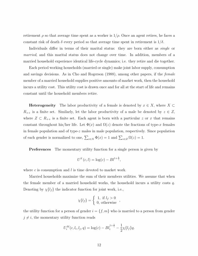
The model economy we consider is populated with males and females who differ in their

labor market productivities, and who exhibit life-cycle behavior. Individuals start economic

life as either married or single and do not change their marital status as they age. They are

born as workers with given, immutable labor market efficiencies, and stochastically transit

into retirement and subsequently to death. Hence, in the model agents differ along their

gender, labor productivity, and marital status. Singles decide how much to work and how

much to save out of their total after-tax income. Married households decide on the labor

hours of each household member, and like singles, how much to save.

A novel feature in our analysis is the explicit modeling of the participation decision of

married females in two-person households, and its interplay with the structure of heterogene-

ity and taxation. We assume that if a married female enters the labor force, the household

faces a utility cost. This cost represents the additional difficulty originating from the need to

better coordinate multiple household activities, potential child-care costs, etc. As a result,

females in married households may choose not to work at all if this utility cost is sufficiently

high, which naturally generates labor supply movements along the extensive margin. This

is a key feature of our analysis since the structure of taxation can affect the participation

decision of married females, and available evidence suggests that it does so significantly. Our

model thus permits us to separate and quantify changes in labor supply that take place at

extensive and intensive margins.

We restrict model parameters so that our benchmark economy is consistent with relevant

aggregate and cross-sectional U.S. data. Three aspects of our parameterization are critical.

First, using data on tax returns we estimate effective tax functions for married and single

households. These functions relate taxes paid to reported incomes, and are able to capture

the complex relation between household’s incomes and taxes in a parsimonious way. Second,

we calibrate our benchmark economy to be consistent both with available estimates of in-

tertemporal elasticities of labor supply along the intensive margin, and with observations on

the labor force participation of married females. In particular, we select parameter values so

that the labor force participation of married females reacts to their own wages as it does in

the data. This aspect of our parameterization is crucial since it allows us to capture the un-

derlying elasticities of labor force participation of married females. Finally, the demographic

structure of the model is tightly mapped to U.S. observations. The marital structure of

the benchmark economy (who is single, who is married, and who is married with whom)

3

reproduces exactly the structure observed in the U.S. Census. This is of importance for our

purposes; different households face different average and marginal tax rates, and reactions

of different households to a tax reform are potentially not the same.

We consider four revenue-neutral tax reforms. Three of these reforms are fundamental

in nature: a proportional consumption tax, a proportional income tax, and a progressive

consumption tax, e.g. Hall and Rabushka (1995), which consists of a single tax rate above

an exemption level. In our last reform (separate filing), we keep the progressivity and the

tax base of the current system intact, but married individuals file taxes separately. This

reform, which arises naturally in our environment, shifts the unit subject to taxation from

households to individuals. As a result, it can drastically change marginal tax rates within

married households, while effectively eliminating tax penalties (and bonuses) associated to

marital status built into the current tax code.

In line with the existing literature, we find that tax reforms can have large effects across

steady states on macroeconomic variables, such as output and capital intensity. A central

finding of our exercises is that the differential labor supply behavior of different groups is

key for an understanding of the aggregate effects of tax reforms. The related finding is that

married females account for a disproportionate fraction of the changes in hours and labor

supply. Furthermore, this fraction increases sharply for low values of the intertemporal

elasticity of labor supply.

Replacing current income taxes by a proportional consumption (income) tax increases the

aggregate output by about 11.2% (5.9%). This increase is accompanied by differential effects

on labor supply: while hours along the intensive margin increase by about 2.7% (2.4%), the

labor force participation of married females increases by about 7.3% (6.2%) and married

females increase their total hours by 10.6% (9.3%). Both reforms have similar effects on

labor supply, which suggests that the flattening of the tax schedule is what really matters

for labor supply behavior. On the other hand, their effects on capital accumulation differ

significantly, which is reflected in how much aggregate output rises.

The effects of a progressive consumption tax reform are different. The aggregate effects

are more moderate and the positive effects on labor force participation of married females are

much less pronounced. If the exemption level associated with the progressive consumption

tax reform is relatively high (higher degree of progressivity), aggregate output increase only

by about 8.0% (as opposed to 11.2% with a proportional consumption tax reform). The rise

4

in the labor force participation of married females is also less pronounced than the propor-

tional consumption tax reform and is only 3.2% (instead of 7.3%). With proportional taxes,

the rise in labor force participation monotonically declines as the productivity of married

females increases. This is not the case for a progressive consumption tax. Females with low

productivity levels change their labor supply very little after a progressive consumption tax

reform. Hence, the way tax reforms affect labor supply of married females depends crucially

of the structure of the particular reform under consideration.

Finally, separate filing goes a long way in generating significant aggregate output effects.

With separate filing, aggregate output goes up by about 2.6%, which is almost half of the

increase from a proportional income tax reform. The increase in aggregate output mainly

comes from the rise in aggregate hours by married females. The labor force participation of

married females rises close to what it does under a proportional income (consumption) tax

reform: an increase of 5.9% versus 6.2% (7.3%). In contrast to other reforms, hours per male

workers are nearly constant, and the increase capital to output ratio is much more moderate.

In answering the first question posed above, “what is the importance of the labor supply

responses of married females in these experiments?”, we find that married females account

for a disproportionate fraction of the changes in hours and labor supply. Under proportional

taxes, married females account for about 58-59% of the total increase in labor hours, and

about 49-50% of the aggregate increase in labor supply (efficiency units). Under progressive

consumption taxes, married females contribute even more significantly to changes in labor

hours and labor supply; in our exercises married females can account for up to 80% and

65% of the total changes in total working hours and labor supply, respectively. Finally, with

separate filing almost all of the rise in hours and labor supply comes from married females,

as their contribution is about 92% of total change in hours and to 89% of the total change

in labor supply.

In answering the second question, “what is the importance micro labor supply elasticities

for the long-run effects on output and the labor input?”, we find that the importance of

married females rises sharply when the parameter governing the intertemporal labor supply

elasticity is lowered from our benchmark value of 0.4 to 0.2. In this case, the contribution

of married females to changes in labor hours is quite higher, ranging from 76% to 98%

across different reforms, and is driven mostly by changes in participation. While the relative

importance of female labor supply becomes much more important, the rise in the total labor

5

input remains relatively constant as we alter the value of the intertemporal labor supply

elasticity. Then, a central finding is that the value of this preference parameter is of second-

order importance in understanding the effects on labor supply associated to tax reforms.

Finally, in terms of the third question, “how do our results compare to those emerging

from a standard (single-earner) macroeconomic model?”, we find that reforms introduced

to a version of our economy that mimics a standard macroeconomic model, generates only

a fraction of the long-run output gains. For a proportional consumption tax, the standard

model generates only 85%-89% of the changes in output implied by our framework. Thus,

tax reform exercises in the context of macroeconomic models with single earners can be

misleading if low labor supply elasticities are used.

Background There are several reasons that point to the relevance of our analysis.

First, in the current U.S. tax system the household (not the individual) constitutes the

basic unit of taxation, which may result in high tax rates on secondary earners. A single

woman’s taxes depend only on her own income. Yet, when a married female considers

entering the labor market, the first dollar of her earned income is taxed at her husband’s

current marginal rate. Second, from a conceptual standpoint, wages of each member in a

two-person household affect joint labor supply decisions as well as the reactions to changes

in the tax structure. Thus, the degree of marital sorting (who is married to whom) could

affect the aggregate responses to alternative tax rules. Finally, a common view among many

economists has been that tax changes may have moderate impacts on labor supply. This

view is supported by empirical findings on the low or near zero labor supply elasticities of

prime-age males. Recent developments, however, started to challenge this wisdom. Tax

reforms in the 1980’s have been shown to affect female labor supply behavior significantly,

but have relatively small effects on males (Bosworth and Burtless (1992), Triest (1990), and

Eissa (1995)). More recently, Eissa and Hoynes (2006) show that the disincentives to work

embedded in the Earned Income Tax Credit (EITC) for married women are quite significant

(effectively subsidizing some married women to stay at home). These findings are consistent

with ample empirical evidence that female labor supply in general, and female labor force

participation in particular are quite elastic (Blundell and MaCurdy (1999)); they point in

the direction of modeling explicitly household labor choices. If households, not individuals,

react to taxes much more than previously thought, the potential effects of tax reforms can

6

be more significant.

Our work largely builds on two main strands of literature. First, our evaluation of tax

reforms using a dynamic model with heterogeneity follows the work by Ventura (1999), Altig,

Auerbach, Kotlikoff, Smetters and Walliser (2001), Castaneda, Dıaz-Jimenez and Rıos-Rull

(2003), Dıaz-Jimenez and Pijoan-Mas (2005), Nishiyama and Smetters (2005), Conesa and

Krueger (2006), and Erosa and Koreshkova (2007) among others. In contrast to these papers,

we study economies populated with married and single households, where married households

can have one or two earners. Chade and Ventura (2002) study the effects of tax reforms

on labor supply and assortative matching in a model with heterogenous individuals and

endogenous marriage decisions. These authors, however, abstract from labor supply decisions

along the extensive margin and capital accumulation.3 Second, as Cho and Rogerson (1988),

Mulligan (2001), and Chang and Kim (2006), we study the aggregate effects of changes in

labor supply along the extensive margin. We differ from these papers by explicitly analyzing

the role of the extensive margin for public policy.4

Our paper is also related to two recent literatures. First, it is related to recent work

that argues that the structure of taxation can significantly affect labor choices, and play a

significant role in accounting for cross-country differences in labor supply behavior. Davis

and Henrekson (2003), Olovsson (2003), Prescott (2004), and Rogerson (2006) are examples

of papers in this group. Our paper is also related to recent work that studies female labor

supply in macroeconomic setups; Jones, Manuelli and McGrattan (2004), Greenwood and

Guner (2004), Greenwood, Seshadri and Yorukoglu (2005), Albanesi and Olivetti (2007),

Attanasio, Low and Sanchez Marcos (2007) and Knowles (2007) are representative papers

in this group.

The paper is organized as follows. Section 2 presents an example that highlights the role

of taxation with two-person households, and motivates the parameterization of the model

economy. Section 3 presents the model economy. Section 4 discusses the parameterization

of the model and the mapping to data. Results from tax reforms are presented in section

5. Section 6 quantifies the role of married females and the extensive margin in labor supply.

3Kleven and Kreiner (2006) study optimal taxation of two-person households when households face anexplicit labor force participation decision.

4See Kaygusuz (2006a, 2006b) for recent analysis of tax and social security policies with an extensivemargin in labor supply. See also Hong and Rıos-Rull (2007) for a recent analysis of the role of social securityin a framework with married and single households.

7

Section 7 discusses the implications of a lower labor supply elasticity. Section 8 compares

the results of our framework with those in a standard macroeconomic model. Section 9

concludes.

2 Taxation, Two-Person Households and the Extensive

Margin

In this section, we present a simple two-period example that illustrates how taxes affect

labor supply decisions with two-earner households, with an emphasis on the effects on the

potential changes in labor force participation. The example serves to highlight key features

of our general environment. It also helps understanding some of the calibration choices we

make later.

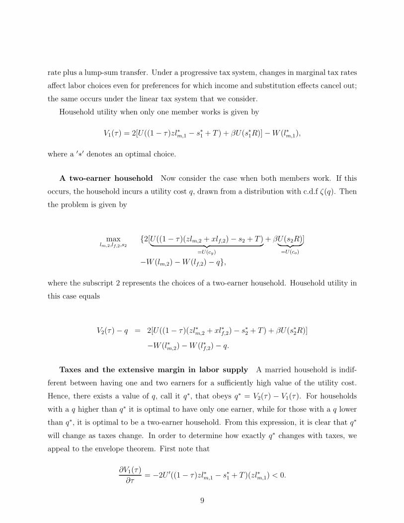
A one-earner household Consider a married household that lives for two periods;

young (y) and old (o). Suppose household members work only in the first period and retire

in the second one. The household decides whether only one or both members should work

in the first period, and how much to save for the retirement. Let R be the gross interest rate

on savings, and let x and z denote the labor market productivities (wage rates) of males and

females, respectively. Let τ be a proportional labor tax on first period’s labor income.

Consider first the problem if only one member (husband) works. The household problem

is given by

maxlm,1,s1

2[U((1 − τ)zlm,1 − s1 + T )︸ ︷︷ ︸=U(cy)

+ βU(s1R)︸ ︷︷ ︸= U(co)

] −W (lm,1),

where lm,1 is the labor choice of the primary earner (husband), s1 are assets for next period

(savings) and T is a transfer received from the government in the first period. The subscript

1 represents the choices of a one-earner household. The functions U(.) and W (.) stand for

the instantaneous utility and disutility, associated to household consumption and worktime,

respectively. Both functions are differentiable; U(.) is strictly concave while W (.) is strictly

convex.

We introduce government transfers in order to capture and illustrate in a simple way the

role of progressive taxation. This follows as household choices under non-linear, progressive

taxes are equivalent to choices under a linear tax system that combines a proportional tax

8

rate plus a lump-sum transfer. Under a progressive tax system, changes in marginal tax rates

affect labor choices even for preferences for which income and substitution effects cancel out;

the same occurs under the linear tax system that we consider.

Household utility when only one member works is given by

V1(τ) = 2[U((1 − τ )zl∗m,1 − s∗1 + T ) + βU(s∗1R)] −W (l∗m,1),

where a ′∗′ denotes an optimal choice.

A two-earner household Now consider the case when both members work. If this

occurs, the household incurs a utility cost q, drawn from a distribution with c.d.f ζ(q). Then

the problem is given by

maxlm,2,lf,2,s2

2[U((1 − τ)(zlm,2 + xlf,2) − s2 + T )︸ ︷︷ ︸=U(cy)

+ βU(s2R)︸ ︷︷ ︸=U(co)

]

−W (lm,2) −W (lf,2) − q,

where the subscript 2 represents the choices of a two-earner household. Household utility in

this case equals

V2(τ ) − q = 2[U((1 − τ)(zl∗m,2 + xl∗f,2) − s∗2 + T ) + βU(s∗2R)]

−W (l∗m,2) −W (l∗f,2) − q.

Taxes and the extensive margin in labor supply A married household is indif-

ferent between having one and two earners for a sufficiently high value of the utility cost.

Hence, there exists a value of q, call it q∗, that obeys q∗ = V2(τ) − V1(τ). For households

with a q higher than q∗ it is optimal to have only one earner, while for those with a q lower

than q∗, it is optimal to be a two-earner household. From this expression, it is clear that q∗

will change as taxes change. In order to determine how exactly q∗ changes with taxes, we

appeal to the envelope theorem. First note that

∂V1(τ)

∂τ= −2U ′((1 − τ)zl∗m,1 − s∗1 + T )(zl∗m,1) < 0.

9

Similarly,

∂V2(τ)

∂τ= −2U ′((1 − τ)(zl∗m,2 + xl∗f,2) − s∗2 + T )(zl∗m,2 + xl∗f,2) < 0.

Henceforth,

∂q∗

∂τ=∂V2(τ )

∂τ−∂V1(τ)

∂τ< 0,

if and only ifU ′((1 − τ )(zl∗m,2 + xl∗f,2) − s∗2 + T )

U ′((1 − τ)zl∗m,1 − s∗1 + T )>

zl∗m,1

zl∗m,2 + xl∗f,2

.

That is, q∗ and as a result, female labor force participation, will be lower when taxes are

high if and only if the above condition holds. Suppose now that U(c) = log(c).5 In this case,

this condition reduces (after some algebra) to

(1 − τ) +T

(zl∗m,1)> (1 − τ ) +

T

(zl∗m,2 + xl∗f,2). (1)

Thus, as long as condition (1) holds, lower (higher) taxes on labor will increase (decrease)

the threshold q∗, and generate a higher (lower) labor force participation of the household’s

secondary earner. This is illustrated in the top panel of Figure 1. Thus, a change in tax

rates affects not only the intensive margin in labor supply but also the extensive margin.

Notice that the above condition necessarily holds in our case. If the transfer and the

marginal tax rate are not contingent on the number of earners in the household (as modeled

here), then for a given household type, the labor income in the two earner case will be higher

than in the first earner case. This follows simply from concavity of the utility function.

We note here three things. First, the fact that the transfer and the marginal tax rate are

not contingent on the number of earners in the household captures U.S. tax rules that take

the household as the unit of taxation. From this perspective, a reduction in the marginal

tax rate on the household is effectively a reduction on the tax rate on secondary earners that

may prompt a movement along the extensive margin. Second, the threshold q∗ changes in

response to changes in the tax rate even under log-preferences for consumption, for which

income and substitution effects usually cancel out. Here, the presence of the common transfer

is essential for the movement in q∗, as condition (1) shows. When a transfer is present, and

5This is our case of interest, as we use it in our general environment.

10

of course more generally under progressive taxation, changes in marginal tax rates affect not

only q∗, but labor supply along the intensive margin. This occurs as income and substitution

effects no longer cancel out.

Finally, from this analysis, changes in labor supply (in efficiency units) in response to

tax rate changes can be decomposed in two parts: there are changes in labor supply from

males and females currently working (intensive margin), and changes due to female labor

force participation (extensive margin). Assuming that couples differ only in terms of utility

cost they face, aggregate labor supply of married couples (L), can be written as

L = ζ(q∗)[zl∗m,2 + xl∗f,2] + (1 − ζ(q∗))zl∗m,1

Hence, the change in aggregate labor supply from tax rate changes is given by

∂L

∂τ= ζ(q∗)[z

∂l∗m,2

∂τ+ x

∂l∗f,2

∂τ] + (1 − ζ(q∗))z

∂l∗m,1

∂τ︸ ︷︷ ︸intensive margin

+ ζ ′(q∗)[zl∗m,2 + xl∗f,2 − zl∗m,1]∂q∗

∂τ︸ ︷︷ ︸extensive margin

. (2)

This example has important implications for the mapping of our model economy to the

data. As the bottom panel of Figure 1 shows, exactly how much the labor force partici-

pation of married females will increase depends on the shape of ζ(q). Therefore, selecting

the functional form for the distribution of utility costs will be a key part of the model pa-

rameterization; the magnitude of the response along the extensive margin depends on slope

ζ ′(q) as equation (2) illustrates. We capture this slope by exploiting the observed changes

in female labor force participation in response to changes in the gender gap, x/z. The key

to this procedure is that an increase in x, for a given z, implies an increase in labor force

participation whose magnitude hinges precisely on the magnitude of ζ ′(q).

3 The Economic Environment

We study a stationary economy populated by a continuum of males and a continuum of

females. The total mass of agents in each gender is normalized to one. As in Gertler

(1999), individuals have finite lives, that are divided in two stages, work and retirement. In

particular, each agent is born as a worker and faces each period a constant probability of

11

retirement ρ so that average time spent as a worker is 1/ρ. Once an agent retires, he faces a

constant risk of death δ every period so that average time spent in retirement is 1/δ.

Individuals differ in terms of their marital status: they are born either as single or

married, and this marital status does not change over time. In addition, members of a

married household experience identical life-cycle dynamics; i.e. they retire and die together.

Each period working households (married or single) make joint labor supply, consumption

and savings decisions. As in Cho and Rogerson (1988), among other papers, if the female

member of a married household supplies positive amounts of market work, then the household

incurs a utility cost. This utility cost is drawn once and for all at the start of life and remains

constant until the household members retire.

Heterogeneity The labor productivity of a female is denoted by x ∈ X, where X ⊂

R++ is a finite set. Similarly, let the labor productivity of a male be denoted by z ∈ Z,

where Z ⊂ R++ is a finite set. Each agent is born with a particular z or x that remains

constant throughout his/her life. Let Φ(x) and Ω(z) denote the fractions of type-x females

in female population and of type-z males in male population, respectively. Since population

of each gender is normalized to one,∑

x∈X Φ(x) = 1 and∑

z∈Z Ω(z) = 1.

Preferences The momentary utility function for a single person is given by

US (c, l) = log(c) −Bl1+1

γ ,

where c is consumption and l is time devoted to market work.

Married households maximize the sum of their members utilities. We assume that when

the female member of a married household works, the household incurs a utility costs q.

Denoting by χlf the indicator function for joint work, i.e.,

χlf =

1, if lf > 00, otherwise

,

the utility function for a person of gender i = f,m who is married to a person from gender

j 6= i, the momentary utility function reads

UMi (c, li, lj, q) = log(c) − Bl

1+ 1

γ

i −1

2χlfq.

12

Note that consumption is a public good within the household. Note also that the parameter

γ > 0 is the intertemporal elasticity of labor supply and is independent of gender and marital

status.

We assume that q ∈ Q, where Q ⊂ R++ is a finite set. We assume that for a given house-

hold, the distribution function for q depends on labor market productivity of the husband.

Let ζ(q|z) denote the probability that the cost of joint work is q, with∑

q∈Q ζ(q|z) = 1

for all z, for a household with male productivity level z. This particular choice for ζ will

become apparent when we discuss our calibration strategy in the next section. At the start

of life, once a particular (x, z) household is formed, the household draws its q, which remains

constant until retirement. We assume that each member of the household incurs half of this

total utility cost.

Production and Markets There are competitive firms that operate a constant returns

to scale technology. Firms rent capital and labor services from households at the rate R and

w, respectively. Using k units of capital and l units of labor, firms produce F (k, l) = kαl1−α

units of consumption good. We assume that the capital depreciates at rate δk.

Households save in the form of a risk-free asset that pays the competitive rate of return

r. There are no markets to insure mortality or retirement risk. We assume that assets of

agents who die are not distributed among those who survive.

Incomes and Taxation Let a represent household’s assets. Then, the total pre-tax

resources of a single working male are given by a + ra + wzl, whereas for a single female

worker they amount to a+ar+wxl. The pre-tax total resources for a married working couple

are given a+ra+wzlm +wxlf . Let bSi and bM indicate the level of social security benefits for

singles, for i = f,m, and married retired households, respectively. Then, retired households

pre-tax resources are simply a + ra + bSi for single retired households, and a + ra + bM for

married ones.

Income for tax purposes, I, is defined as total labor and capital income; hence for a

single male worker I = ra + wzl, while for a single female worker I = ra + wxl. For a

married working household, taxable income equals I = ra + wzlm + wxlf . We assume that

social security benefits are not taxed, so the income for tax purposes is simply given by ra

for retired households. The total income tax liabilities of married and single households are

13

represented by tax functions TM(I) and T S(I), respectively. These functions are continuous

in I, increasing and convex. There is also a (flat) payroll tax that taxes individual labor

incomes, represented by τ p, to fund social security transfers. Besides the income and payroll

taxes, each household pays an additional flat capital income tax for the returns from his/her

asset holdings, denoted by τk.

Demographics Let M(x, z) denote the number of marriages between a type-x female

worker and a type-z male worker, and let ω(z) and φ(x) denote the number of single type-z

male workers and the number of single type-x female workers, respectively. Let M r(x, z),

ωr(z) and φr(x) denote the similar quantities for retirees. Then, the following two accounting

identities

Φ(x) ≡∑

z

M(x, z) + φ(x) +∑

z

M r(x, z) + φr(x), (3)

and

Ω(z) ≡∑

x

M(x, z) + ω(z) +∑

x

M r(x, z) + ωr(z), (4)

hold by construction. Agents who die (married or single) are replaced by identical young

agents, who are born with no assets. This implies that every period, δM r(x, z) working

married couples are born; the corresponding numbers for singles are δφr(x) and δωr(z).

Note that the law of motion for the number of retired married people reads

M r′(x, z) = (1 − δ)M r(x, z)︸ ︷︷ ︸surviving retired couples

+ ρM(x, z)︸ ︷︷ ︸newly retired couples

, (5)

which implies the following steady state condition

δM r(x, z) = ρM(x, z). (6)

Therefore, in a steady state retired couples who die must be replaced by retiring couples

of the same type. Similarly, for single retired males and females, the following steady state

relations must hold

δφr(x) = ρφ(x), (7)

and

δωr(z) = ρω(z). (8)

14

Equations (6), (7) and (8) imply that the number of working agents, married and single,

are constant over time. Using the steady state restrictions implied by equations (6), (7) and

(8), we can rewrite equation (3) as

Φ(x) =∑

z

M(x, z) +ρ

δ

∑

z

M(x, z) + φ(x) +ρ

δφ(x). (9)

This equation restricts how Φ(x), M(x, z), and φ(x) are related. Similarly, the steady

state version of equation (4) is given by

Ω(z) =∑

x

M(x, z) +ρ

δ

∑

x

M(x, z) + ω(z) +ρ

δω(z). (10)

When we parameterize the model (see below), our strategy is to treat Φ(x), Ω(z), and

M(x, z) as the primitives and select φ(x) and ω(z) to satisfy the stationarity assumption.

Hence, these two equations allow us to pin down φ(x) and ω(z) given the data on Φ(x),

Ω(z), and M(x, z).

The Problem of a Single Household We now define problems of single and married

households recursively. First, consider the problem of a retired single agent and without loss

of generality focus on the problem of a single retired male with asset level a. A single retired

male simply decides how much to save, a′, and his problem is given by

V S,rm (a) = max

a′≥0Us(c, 0) + (1 − δ)βV S,r

m (a′), (11)

subject to

c+ a′ = a(1 + r) + bSm − T S(ra) − τ kra.

The value of being a single retired female with assets a, V S,rf (a), is defined in a similar way.

Let aS,rj (a), for j = f,m, be the decision rules for retired single agents.

Consider now the problem of a single male worker of type (z, a). A single worker of type-

(z, a) decides how much to work and how much to save, taking into account the retirement

probability, ρ. His problem is given by

V Sm(z, a) = max

a′,lSm

US(c, lSm) + β[(1 − ρ)V Sm(z, a′) + ρV S,r

m (a′)], (12)

subject to

c+ a′ = a(1 + r) + wzlSm(1 − τp) − T S(wzlSm + ra) − τkra,

15

and

lSm ≥ 0, a′ ≥ 0.

The value of being a single female worker V Sf (x, a) can be defined in a similar fashion.

Again, let aSf (x, a) and aS

m(z, a) represent the savings decisions for single females and males,

respectively, and let lSf (x, a) and lSm(z, a) be their labor supply decision rules.

The Problem of Married Households Again, consider first the problem of a retired

couple with assets a. Their problem, with the associated decision rule aM,r(a), is given by

V M,r(a) = maxa′≥0

UMm (c, 0, 0, q) + UM

f (c, 0, 0, q) + (1 − δ)βV M,r(a′), (13)

subject to

c+ a′ = a(1 + r) + bM − TM(ra) − τkra.

Consider now the problem of a married working household of type (x, z, a, q). A married

working household solves a joint maximization problem by choosing consumption, next-

period assets and labor supply for each household member. The problem is given by

V M(x, z, a, q) = maxa′, lM

f, lMm

[UMm (c, lMm , l

Mf , q) + UM

f (c, lMm , lMf , q)] (14)

+ β[(1 − ρ)V M(x, z, a′, q) + ρV M,r(a′)],

subject to

c+ a′ = a(1 + r) + w(zlMm + xlMf )(1 − τp) + ra− TM(wzlMm + wxlMf + ra) − τkra,

and

lMm ≥ 0, lMf ≥ 0, a′ ≥ 0.

Like singles, a married couple decides how much to work and how much to save. Unlike

singles, they might choose zero market hours for female member of the household. This

will occur if q is too high, given the productivity levels x and z and asset holdings a. Let

lMf (x, z, a, q), lMm (x, z, a, q), and aM(x, z, a, q) represent the optimal decision rules associated

with this problem.

16

Aggregate Consistency The aggregate state of this economy consists of distribution

of households over their types and asset levels. Suppose a ∈ A = [0, a]. Consider first

workers. Let ψM(B, x, z, q) be the number (measure) of working married households of type

(x, z, q), with assets B ∈ A, the class of Borel subsets of A. Similarly, let ψSf (B, x) be the

number of working single females of type x, with a ∈ B, and let ψSm(B, z) be the number

of single working males of type (z), with a ∈ B. By construction, M(x, z), the number of

married working households of type (x, z), must satisfy

M(x, z) =∑

q

∫

A

ψM(a, x, z, q)da.

Similarly, the number of single households (agents) must be consistent with ψSf (x, a) and

ψSm(z, a), i.e. φ(x) and ω(z) must satisfy

φ(x) =

∫

A

ψSf (a, x)da,

and

ω(z) =

∫

A

ψSm(a, z)da.

Since retired agents are not allowed to work, they only differ by their marital status and

asset holdings. Let ψM,r(B), ψS,rf (B) and ψS,r

m (B) denote the asset distribution among retired

married, retired single female and retired single male households, respectively with a ∈ B.

Like their counterparts for workers, these distributions must be consistent with M r(x, z),

φr(x) and ωr(z).

Equilibrium In stationary equilibrium, factor markets clear, so aggregate capital (K)

and aggregate labor (L) are given by

K =∑

x, z, q

∫

A

aψM(a, x, z, q)da+∑

z

∫

A

aψSm(a, z)da+

∑

x

∫

A

aψSf (a, x)da

+

∫

A

aψM,r(a)da+

∫

A

aψS,rm (a)da+

∫

A

aψS,rf (a)da,

and

17

L =∑

x, z, q

∫

A

(xlMf (a, x, z, q) + zlMm (a, x, z, q))ψM(a, x, z, q)da+

∑

z

∫

A

zlSm(a, z)ψSm(a, z)da+

∑

x

∫

A

xlSf (a, x)ψSf (a, x)da.

In addition, factor prices are competitive so w = F2(K,L), R = F1(K,L), and r = R−δk.

In the Appendix, we provide a formal definition of equilibria.

4 Parameter Values

We now proceed to assign parameter values to the endowment, preference and technology

parameters of our benchmark economy. To this end, we use cross-sectional, aggregate as

well as demographic data. As a first step in this process, we start by defining the length of

a period to be a year.

Demographics and Endowments We assume that agents are workers for forty years,

corresponding to ages 25 to 64, and set ρ = 1/40 accordingly. Absent population growth

in the model, we set δ so that the model is consistent with the observed fraction of retired

individuals (65 years and above), as a fraction of the population 25 years and older. From

the 2000 Census, we calculate that this fraction was 0.203. Hence, given the value assumed

for ρ, we set δ equal to 0.0982 in order to reproduce the same age structure in the benchmark

economy.

We set the number of productivity types (labor endowments) to five. Each productivity

type corresponds to an educational attainment level: less than high school (< hs), high

school (hs), some college (sc), college (col) and post-college education (> col). We use data

from the Consumer Population Survey (CPS) to calculate efficiency levels for all types of

agents. Efficiency levels correspond to mean hourly wage rates within an education group,

which we construct using annual wage and salary income, weeks worked, and usual hours

worked data.6 We include in the sample household heads and spouses between 25 and 54,

and exclude those who are self-employed or unpaid workers. Table 1 shows the estimated

efficiency levels for the corresponding types, where wage rates for each type and gender are

6We find the mean hourly wages as annual wage and salary income(usual hours worked)(number of weeks worked) .

18

normalized by the overall mean hourly wages in the sample. The Table also reports the

observed gender gap in hourly wage rates for each educational group; the gap is roughly

constant across educational categories, averaging about 72%.

We subsequently determine the distribution of individuals by productivity types for each

gender, i.e. Ω(z) and Φ(x), using the 2000 Census. For this purpose, we assume an under-

lying stationary demographic data, and assume that the distribution of retired agents by

educational attainment is the same as the observed distribution of agents prior to retirement.

Given this assumption, we consider all household heads or spouses who are between ages 25

and 64 and for each gender calculate the fraction of population in each education cell. For

the same age group, we also construct M(x, z), the distribution of married working couples,

as shown in Table 2. Consistent with positive assortative matching by education, the largest

entries in each row and column in Table 2 are located along the diagonal.7

Finally, given the fractions of individuals in each education group, Φ(x) and Ω(z), and

the fractions of married working households, M(x, z), in the data, we calculate the implied

fractions of single working households, ω(z) and φ(x), reported in Table 3. About 74% of

households in the benchmark economy consists of married households, while the rest (about

26%) are single-person ones. This table also shows ω(z) and φ(x) that we construct from

the 2000 Census. The mismatch between implied and actual values of ω(z) and φ(x) is quite

small, suggesting that stationary population structure is not an unrealistic assumption.

Technology We specify the production function as Cobb-Douglas with capital share

equal to 0.317. In the absence of population growth and growth in labor efficiency, we set

the depreciation rate equal to 0.07. These values are consistent with a notion of capital that

excludes residential capital, consumer durables and government owned capital for the period

1960-2000. The corresponding notion of output is then GDP accounted for by the business

sector. Altogether, this implies a capital to output ratio of about 2.325.8

Taxation To construct income tax functions for married and single individuals, we

estimate effective taxes paid by married and single households as a function of their reported

7See Fernandez, Guner and Knowles (2005) for a recent theoretical and empirical study of positive assor-tative matching by education.

8See Guner, Ventura and Yi (2007) for details.

19

income. We use tabulated data from the Internal Revenue Service by income brackets.9 For

each income bracket, total income taxes paid, total income earned, number of taxable returns

and number of returns data are publicly available. Using these, we find the mean income

and the average tax rate corresponding to every income bracket. We calculate the average

tax rates as

average tax rate = total amount of income tax paid

number of taxable returns

total adjusted gross income

number of returns

.

Following Gouveia and Strauss (1994), we then estimate the effective tax functions both for

married and single households. In particular, we fit the following equation to the data,

average tax rate (income) = η1 + η2 log(income) + ε,

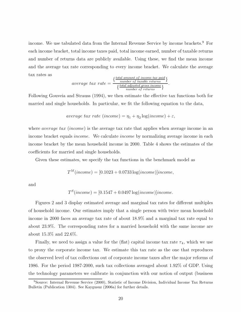
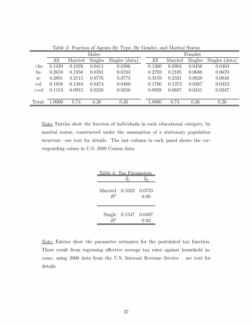
where average tax (income) is the average tax rate that applies when average income in an

income bracket equals income. We calculate income by normalizing average income in each

income bracket by the mean household income in 2000. Table 4 shows the estimates of the

coefficients for married and single households.

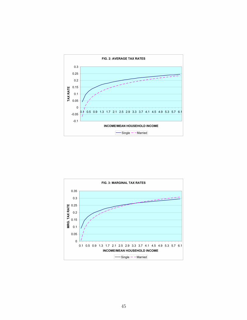
Given these estimates, we specify the tax functions in the benchmark model as

TM(income) = [0.1023 + 0.0733 log(income)]income,

and

T S(income) = [0.1547 + 0.0497 log(income)]income.

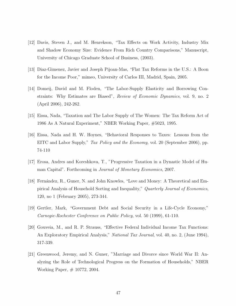
Figures 2 and 3 display estimated average and marginal tax rates for different multiples

of household income. Our estimates imply that a single person with twice mean household

income in 2000 faces an average tax rate of about 18.9% and a marginal tax rate equal to

about 23.9%. The corresponding rates for a married household with the same income are

about 15.3% and 22.6%.

Finally, we need to assign a value for the (flat) capital income tax rate τ k, which we use

to proxy the corporate income tax. We estimate this tax rate as the one that reproduces

the observed level of tax collections out of corporate income taxes after the major reforms of

1986. For the period 1987-2000, such tax collections averaged about 1.92% of GDP. Using

the technology parameters we calibrate in conjunction with our notion of output (business

9Source: Internal Revenue Service (2000), Statistic of Income Division, Individual Income Tax ReturnsBulletin (Publication 1304). See Kaygusuz (2006a) for further details.

20

GDP), we obtain τk = 0.124. In the benchmark economy total taxes, income taxes on labor

and capital and the additional tax on capital, amount to 13.1% of aggregate output.

Social Security We calculate τp = 0.086, as the average value of the social security

contributions as a fraction of aggregate labor income for 1990-2000 period.10 Using Social

Security Beneficiary Data, we calculate that during this same period a retired single woman

obtained old-age benefits of about 0.77 of a single retired male, while a retired couple averaged

benefits of about 1.5 times those of a retired single male. Thus, given the payroll tax rate,

the value of the benefit for a single retired male, bSm, balances the budget for the social

security system.

Preferences There are two utility functions parameters, the intertemporal elasticity of

labor supply (γ) and the parameter governing the disutility of market work (B). We consider

two values for γ: a low value of 0.2 and a higher value of 0.4. Both values are consistent with

recent estimates for males. While γ = 0.2 is in line with microeconomic evidence reviewed

by Blundell and MaCurdy (1999), γ = 0.4 is contained in the range of recent estimates

by Domeij and Floden (2006, Table 5). Domeij and Floden (2006) results are based upon

estimates for married males that control for the bias emerging from borrowing constraints.11

We proceed by presenting first results when the intertemporal elasticity of substitution equals

0.4. In subsequent sections, we discuss the implications of a lower value for this parameter.

Given γ, we select the parameter B to reproduce average market hours per worker observed

in the data. These average hours per worker amounted to about 40.8% of available time in

2000.12

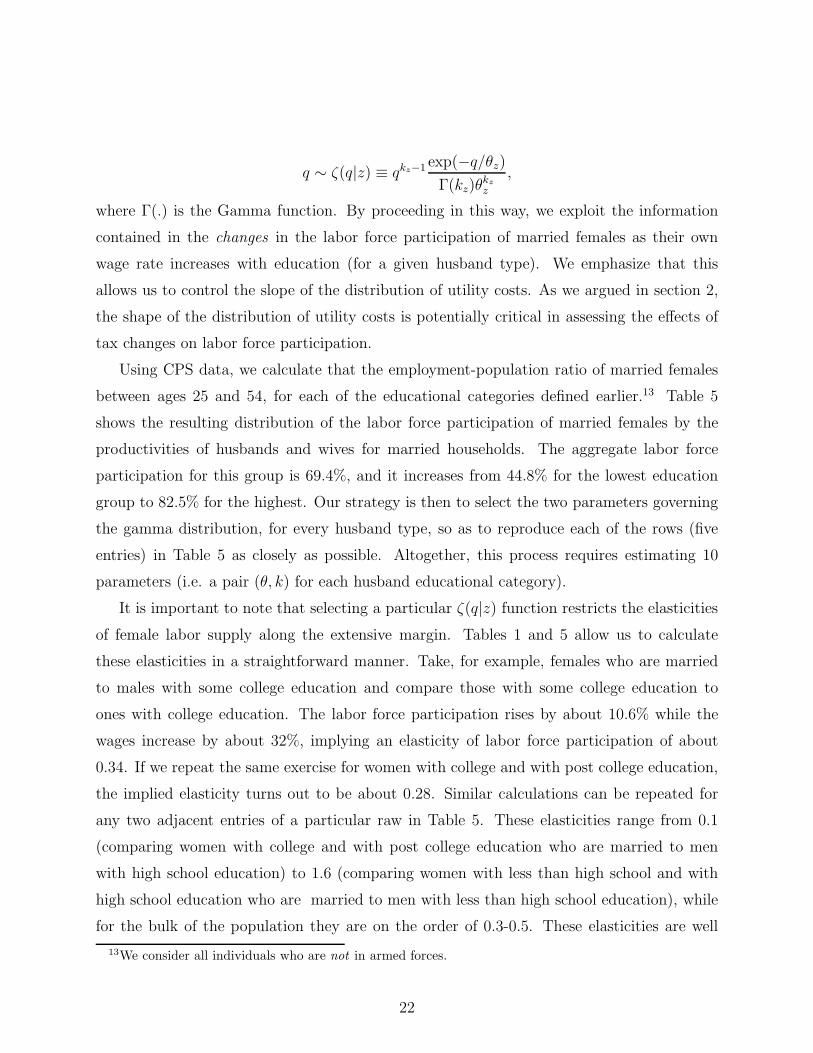
We assume that the utility cost parameter is distributed according to a (flexible) gamma

distribution, with parameters kz and θz. Thus, conditional on the husband’s type z,

10The contributions considered are those from the Old Age, Survivors and DI programs. The Data comesfrom the Social Security Bulletin, Annual Statistical Supplement, 2005, Tables 4.A.3.

11Rupert, Rogerson and Wright (2000) provide estimates within a similar range in the presence of a homeproduction margin. Heathcote, Storesletten and Violante (2007) report an estimate of 0.2, using a modelwith incomplete markets.

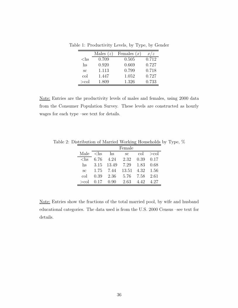
12The numbers are for people between ages 25 and 54 and are based on data from the Consumer PopulationSurvey. We find mean yearly hours worked by all males and females by multiplying usual hours worked ina week and number of weeks worked. Married males work 2294 hours per year, and married females work1741 hours per year. We assume that each person has an available time of 5000 hours per year. Our targetfor hours corresponds to 2040 hours per-year.

21

q ∼ ζ(q|z) ≡ qkz−1 exp(−q/θz)

Γ(kz)θkz

z

,

where Γ(.) is the Gamma function. By proceeding in this way, we exploit the information

contained in the changes in the labor force participation of married females as their own

wage rate increases with education (for a given husband type). We emphasize that this

allows us to control the slope of the distribution of utility costs. As we argued in section 2,

the shape of the distribution of utility costs is potentially critical in assessing the effects of

tax changes on labor force participation.

Using CPS data, we calculate that the employment-population ratio of married females

between ages 25 and 54, for each of the educational categories defined earlier.13 Table 5

shows the resulting distribution of the labor force participation of married females by the

productivities of husbands and wives for married households. The aggregate labor force

participation for this group is 69.4%, and it increases from 44.8% for the lowest education

group to 82.5% for the highest. Our strategy is then to select the two parameters governing

the gamma distribution, for every husband type, so as to reproduce each of the rows (five

entries) in Table 5 as closely as possible. Altogether, this process requires estimating 10

parameters (i.e. a pair (θ, k) for each husband educational category).

It is important to note that selecting a particular ζ(q|z) function restricts the elasticities

of female labor supply along the extensive margin. Tables 1 and 5 allow us to calculate

these elasticities in a straightforward manner. Take, for example, females who are married

to males with some college education and compare those with some college education to

ones with college education. The labor force participation rises by about 10.6% while the

wages increase by about 32%, implying an elasticity of labor force participation of about

0.34. If we repeat the same exercise for women with college and with post college education,

the implied elasticity turns out to be about 0.28. Similar calculations can be repeated for

any two adjacent entries of a particular raw in Table 5. These elasticities range from 0.1

(comparing women with college and with post college education who are married to men

with high school education) to 1.6 (comparing women with less than high school and with

high school education who are married to men with less than high school education), while

for the bulk of the population they are on the order of 0.3-0.5. These elasticities are well

13We consider all individuals who are not in armed forces.

22

within the available empirical estimates. Eissa (1995), using 1986 tax reform as a natural

experiment, estimates an elasticity with respect to the after-tax wage of approximately 0.8

and claims that at least half of the responsiveness is on the participation margin. Triest

(1990) estimates an uncompensated wage elasticities for married women on the order of

0.86-1.12, and suggests that almost all action comes from the extensive margin.

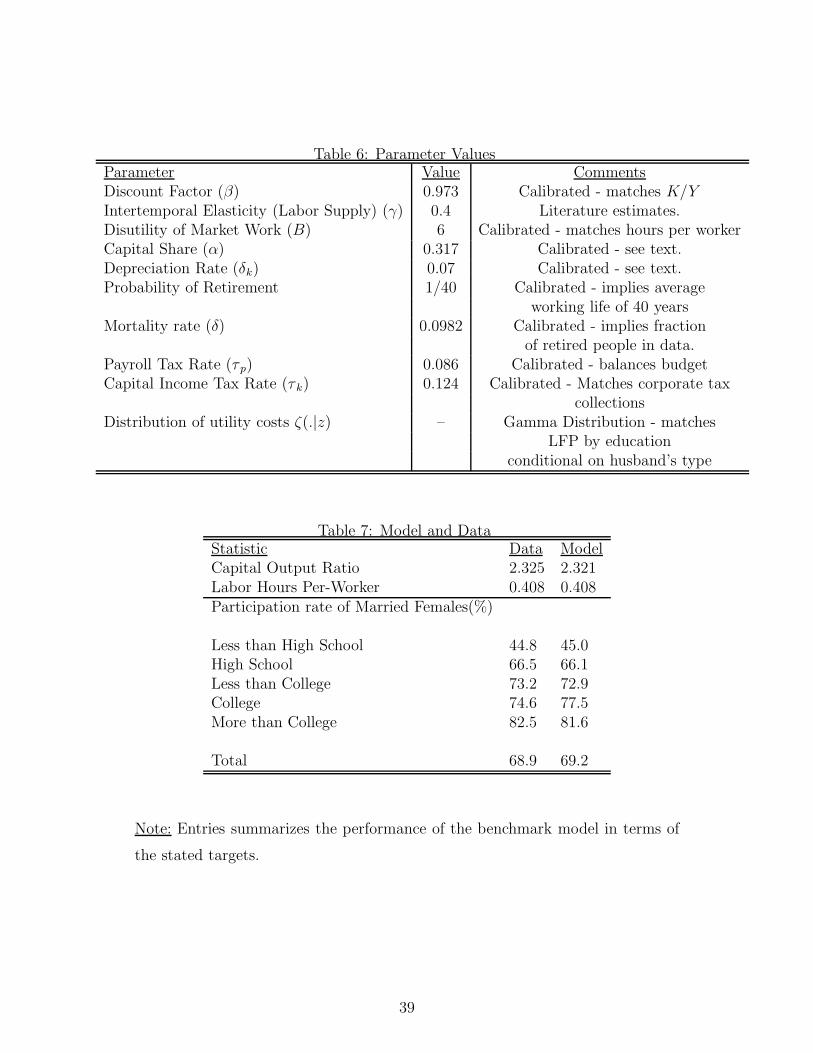
Finally, we choose the remaining preference parameter, the discount factor β, so that the

steady-state capital to output ratio matches the value in the data consistent with our choice

of the technology parameters (2.325). Table 6 summarizes our parameter choices. Table 7

shows the performance of the benchmark model in terms of the targets we impose for B and

β, i.e. labor hours per-worker and capital output ratio. The table also shows how well the

benchmark calibration matches the labor force participation of married females. Although,

as we explained above, our calibration strategy is to match each row of Table 5, it is more

instructive to look at the aggregate participation rate of married females and the labor force

participation of married females by their educational level. The model has no problem in

reproducing jointly these observations as the table demonstrates.

5 Tax Reforms

We now consider four hypothetical reforms to the current U.S. tax structure: a proportional

consumption tax, a proportional income tax, a progressive consumption tax, and a move from

joint to separate filing for married couples. The first reform flattens the current income tax

schedule and changes the tax base from income to consumption, effectively eliminating the

taxation of capital income built into the income tax. The second reform only flattens the tax

schedule while keeping income as the tax base. The third reform reintroduces progressivity

into a consumption tax system. Finally, the last reform changes the unit of taxation from

households to individuals.

The findings we report are based on steady state comparisons of pre and post-reform

economies. In all reforms, we keep the additional tax rate on capital income (τ k) and the

social security system unchanged.14 The exercises are in all cases revenue neutral.

14Results when the tax rate on capital income is also eliminated are available upon request.

23

A Proportional Consumption Tax The first reform replaces current income taxes

with a proportional consumption tax, which makes marginal and average tax rates equal for

all households. For a better understanding of the results, the reader should bear in mind that

a consumption tax still distorts labor choices, but by construction eliminates the distortions

on capital accumulation created by the income tax.

Table 8 reports key findings from this exercise. In line with the existing literature, the

effects of a consumption tax on aggregates are dramatic. Aggregate output increases by

about 11.2%. As a result, a flat consumption tax of 17.8% is all that is needed to generate

revenue neutrality. The long-run rise in output is fueled by significant rises in factor inputs.

The capital-to-output ratio increases by about 15% in the post-reform steady state. Total

(raw) hours in turn increase by 4.7%, while labor supply (hours adjusted by efficiency units)

increases by 4.2%. Despite the rise in labor supply, as a result of higher capital stock in

post-reform economy, the wage rate increases by 6.5% as well.

Our economy allows us to identify and quantify differential responses in labor supply to

tax changes that takes place at the intensive margin for both males and females, as well as

at the extensive margin for married females. Recall that in the benchmark economy, the

tax structure generates non-trivial disincentives to work since marginal tax rates increase

with incomes. In particular, married females who decide to enter the labor force are taxed

at their partner’s current marginal tax rate. With the elimination of these disincentives, in

conjunction with the partial removal of capital income taxation, the change in labor supply of

married females is substantially larger than the aggregate change in hours. The introduction

of a consumption tax implies that the labor force participation of married females increases

by 7.3%, while hours per worker rise by about 2.6% for females, and about 2.8% for males.

Due to changes along the intensive and the extensive margin, total hours for married females

increase by about 10.6%. This is a dramatic rise and is more than three times the change

in total male hours. These results are especially worth noting as the parameter governing

intertemporal substitution of labor is the same for males and females.

A Proportional Income Tax The second reform is similar to the first one but in-

troduces a proportional income tax instead of a proportional consumption tax. The conse-

quences of this reform could then be viewed as the consequences of simply flattening-out the

current income tax schedule.

24

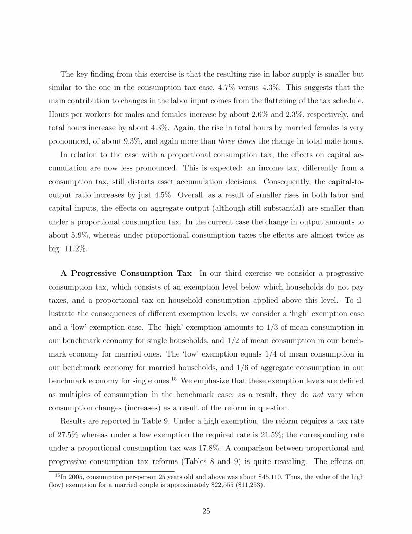
The key finding from this exercise is that the resulting rise in labor supply is smaller but

similar to the one in the consumption tax case, 4.7% versus 4.3%. This suggests that the

main contribution to changes in the labor input comes from the flattening of the tax schedule.

Hours per workers for males and females increase by about 2.6% and 2.3%, respectively, and

total hours increase by about 4.3%. Again, the rise in total hours by married females is very

pronounced, of about 9.3%, and again more than three times the change in total male hours.

In relation to the case with a proportional consumption tax, the effects on capital ac-

cumulation are now less pronounced. This is expected: an income tax, differently from a

consumption tax, still distorts asset accumulation decisions. Consequently, the capital-to-

output ratio increases by just 4.5%. Overall, as a result of smaller rises in both labor and

capital inputs, the effects on aggregate output (although still substantial) are smaller than

under a proportional consumption tax. In the current case the change in output amounts to

about 5.9%, whereas under proportional consumption taxes the effects are almost twice as

big: 11.2%.

A Progressive Consumption Tax In our third exercise we consider a progressive

consumption tax, which consists of an exemption level below which households do not pay

taxes, and a proportional tax on household consumption applied above this level. To il-

lustrate the consequences of different exemption levels, we consider a ‘high’ exemption case

and a ‘low’ exemption case. The ‘high’ exemption amounts to 1/3 of mean consumption in

our benchmark economy for single households, and 1/2 of mean consumption in our bench-

mark economy for married ones. The ‘low’ exemption equals 1/4 of mean consumption in

our benchmark economy for married households, and 1/6 of aggregate consumption in our

benchmark economy for single ones.15 We emphasize that these exemption levels are defined

as multiples of consumption in the benchmark case; as a result, they do not vary when

consumption changes (increases) as a result of the reform in question.

Results are reported in Table 9. Under a high exemption, the reform requires a tax rate

of 27.5% whereas under a low exemption the required rate is 21.5%; the corresponding rate

under a proportional consumption tax was 17.8%. A comparison between proportional and

progressive consumption tax reforms (Tables 8 and 9) is quite revealing. The effects on

15In 2005, consumption per-person 25 years old and above was about $45,110. Thus, the value of the high(low) exemption for a married couple is approximately $22,555 ($11,253).

25

capital intensity are comparable under both types of reforms. This should not be surprising

since the bulk of capital is owned by households who are above the exemption levels and they

are affected in a similar way in these reforms; both reforms eliminate the distorting effects

of income taxes on their asset accumulation decisions. The effect on aggregate output in

the long run, however, is now lower than under a proportional consumption tax and declines

steeply with increases in exemption levels. This is clearly due to the smaller increases in

the labor input. Note that hours and the labor input increase by about 1.5% with the high

exemption level and 3.6-3.2% with the low one, whereas the increase was about 4.7% and

4.2%, respectively, under a proportional consumption tax.

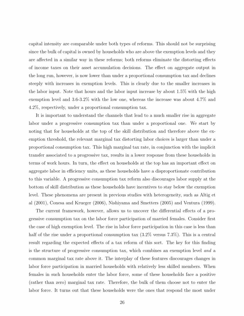
It is important to understand the channels that lead to a much smaller rise in aggregate

labor under a progressive consumption tax than under a proportional one. We start by

noting that for households at the top of the skill distribution and therefore above the ex-

emption threshold, the relevant marginal tax distorting labor choices is larger than under a

proportional consumption tax. This high marginal tax rate, in conjunction with the implicit

transfer associated to a progressive tax, results in a lower response from these households in

terms of work hours. In turn, the effect on households at the top has an important effect on

aggregate labor in efficiency units, as these households have a disproportionate contribution

to this variable. A progressive consumption tax reform also discourages labor supply at the

bottom of skill distribution as these households have incentives to stay below the exemption

level. These phenomena are present in previous studies with heterogeneity, such as Altig et

al (2001), Conesa and Krueger (2006), Nishiyama and Smetters (2005) and Ventura (1999).

The current framework, however, allows us to uncover the differential effects of a pro-

gressive consumption tax on the labor force participation of married females. Consider first

the case of high exemption level. The rise in labor force participation in this case is less than

half of the rise under a proportional consumption tax (3.2% versus 7.3%). This is a central

result regarding the expected effects of a tax reform of this sort. The key for this finding

is the structure of progressive consumption tax, which combines an exemption level and a

common marginal tax rate above it. The interplay of these features discourages changes in

labor force participation in married households with relatively less skilled members. When

females in such households enter the labor force, some of these households face a positive

(rather than zero) marginal tax rate. Therefore, the bulk of them choose not to enter the

labor force. It turns out that these households were the ones that respond the most under

26

proportional tax reforms; as we discuss in detail below. When we lower the exemption level,

the number of households that face this trade-off becomes smaller, and the results look more

similar to the ones obtained under a proportional consumption tax reform.

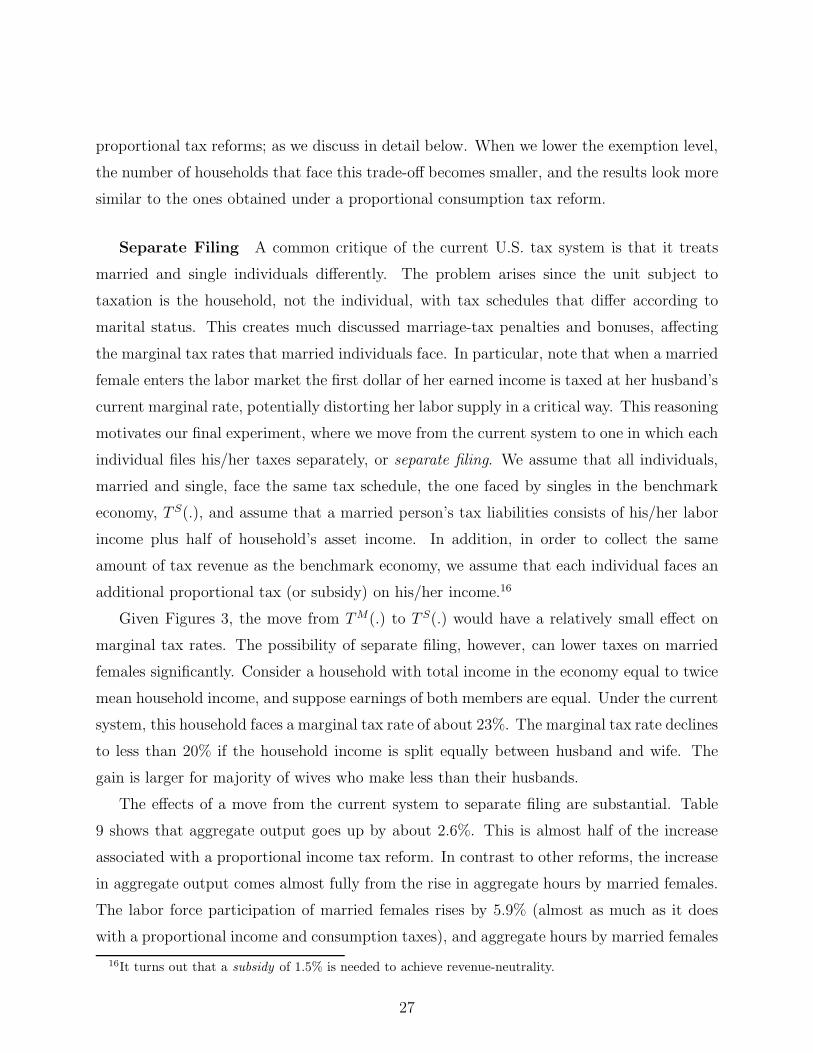
Separate Filing A common critique of the current U.S. tax system is that it treats

married and single individuals differently. The problem arises since the unit subject to

taxation is the household, not the individual, with tax schedules that differ according to

marital status. This creates much discussed marriage-tax penalties and bonuses, affecting

the marginal tax rates that married individuals face. In particular, note that when a married

female enters the labor market the first dollar of her earned income is taxed at her husband’s

current marginal rate, potentially distorting her labor supply in a critical way. This reasoning

motivates our final experiment, where we move from the current system to one in which each

individual files his/her taxes separately, or separate filing. We assume that all individuals,

married and single, face the same tax schedule, the one faced by singles in the benchmark

economy, T S(.), and assume that a married person’s tax liabilities consists of his/her labor

income plus half of household’s asset income. In addition, in order to collect the same

amount of tax revenue as the benchmark economy, we assume that each individual faces an

additional proportional tax (or subsidy) on his/her income.16

Given Figures 3, the move from TM(.) to T S(.) would have a relatively small effect on

marginal tax rates. The possibility of separate filing, however, can lower taxes on married

females significantly. Consider a household with total income in the economy equal to twice

mean household income, and suppose earnings of both members are equal. Under the current

system, this household faces a marginal tax rate of about 23%. The marginal tax rate declines

to less than 20% if the household income is split equally between husband and wife. The

gain is larger for majority of wives who make less than their husbands.

The effects of a move from the current system to separate filing are substantial. Table

9 shows that aggregate output goes up by about 2.6%. This is almost half of the increase

associated with a proportional income tax reform. In contrast to other reforms, the increase

in aggregate output comes almost fully from the rise in aggregate hours by married females.

The labor force participation of married females rises by 5.9% (almost as much as it does

with a proportional income and consumption taxes), and aggregate hours by married females

16It turns out that a subsidy of 1.5% is needed to achieve revenue-neutrality.

27

increase by 7.3%. In contrast, hours by male workers are nearly constant. The main mes-

sage from this experiment is quite clear. A move from the current system to one in which

individuals (not households) are the basic unit of taxation, goes a long way in generating

significant effects on aggregate labor and output. Note that this occurs without eliminating

tax progressivity, or the taxation of capital income.

Discussion The analysis so far reveals several important insights that a single-agent

framework would fail to capture. Notice that female labor force participation plays a sig-

nificant role in all of the reforms we have considered. Under proportional taxes, the overall

rise in married female hours is more than three times the rise in male hours, and fueled by a

significant increase in the extensive margin. Furthermore, the structure of reforms interact

in a nontrivial way with the labor force participation of married females. The increases in the

labor force participation, as well as aggregate hours of married females, under a progressive

consumption tax reform can be much lower than those under a proportional consumption

tax reform. Overall, these findings motivate us to explicitly quantify the relative importance

of married females for our results. We do this in the next section.

6 The Role of Married Females

We now discuss in detail the changes in labor supply of married females. We ask: what is the

overall contribution of married females to changes in labor supply? What is the importance

of labor supply changes along the extensive margin?

In answering these questions, we first note that the type of the tax reform under consider-

ation is critical. Although the aggregate effects on labor supply are smaller under progressive

consumption tax relative to a proportional one, the rise in married females’s labor supply

becomes a much more important component of the overall rise in labor supply (i.e. labor

in efficiency units). Furthermore, the role of married females is largest with a move to sep-

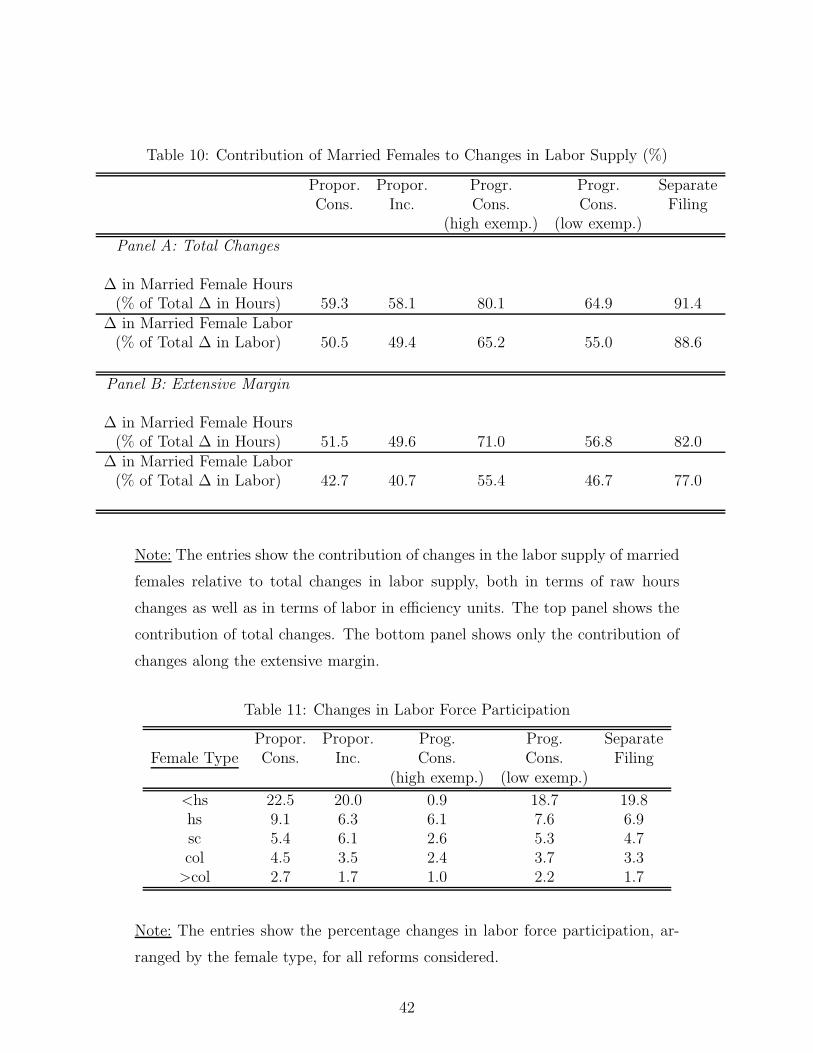
arate filing. Table 10 makes these points clear. In this table we report the contribution

of married females to changes in total hours and total labor supply under our benchmark

calibration. For proportional consumption and income taxes, the contribution of married fe-

males to changes in total hours is around 58-59%. Nevertheless, the contribution of married

females to changes in total hours is much higher under a progressive consumption tax: about

28

65% and 80% for the low and high exemption values, respectively. This occurs as changes

in labor supply for other groups are of smaller or negative magnitude under a progressive

consumption tax.17 Married females’ contributions are largest in separate filing reform; they

contribute to more than 90% of changes in total hours. The contributions of married females

to total labor supply follow a similar pattern, but the magnitudes are smaller. This occurs

since females on average are less skilled than men, and since the rise in female labor supply

is concentrated among low skilled ones, an issue that we elaborate below. The results in

Table 10 indicate that married females account for about 49-50% of the changes in labor

supply under proportional taxes, about 55% and 65% of the changes under a progressive

consumption tax, and almost about 90% under separate filing. We conclude that the overall

contribution of married females is substantial; they contribute disproportionately to changes

in labor supply given their share of the working age population (about 37.5%).

In the bottom panel of Table 10 we focus on the role of the extensive margin and report

its contribution to the rise in hours and total labor supply. In order to calculate the role of

extensive margin, we count both the hours worked by married females who enter the labor

market, as well as by those who stop participating. The latter is necessary as some married

females, in particular those with low skills after a progressive consumption tax reform, prefer

not to work in the post-reform economy. Concretely, for each (x, z, a, q)-type married woman,

we first determine if labor force participation for this type is different between pre and post

reform economies. If the change in participation is positive and a married woman enters

the labor force after a reform, we weigh the change in participation by the hours she works

(or the total labor she supplies) under the new tax system. Summing up over all such

households gives us the total rise in hours (or in labor supply) due to extensive margin. If,

on the other hand, the change is negative and a married woman stops working, we weigh

the change in participation by the hours she worked (or total labor she supplied) in the

benchmark economy. The difference between these two sums gives us the net change in

hours (or total labor supply) due to the extensive margin. Using this measure, the extensive

margin contributes about 49-51% of the changes in total hours under proportional taxes,

about 57% and 71% of the changes under progressive taxes, and about 77% under separate

17The interplay of high marginal tax rates and an exemption value, dictates that the bulk of singleindividuals decrease hours worked after the reform in the high exemption case. For single females, onlythose with college education increase hours (0.2%). For single males, an increase in hours takes place forthose with college education or above (0.6% and 0.8%, respectively).

29

filing. For changes in labor supply, the contributions are 41-43%, about 47% and 55%, and

about 82% respectively. By this measure, these calculations suggest that the bulk of the

rise in the labor supply of married females can be attributed to movements in the extensive

margin.

A central finding emerging from our proportional tax exercises is that the increase in

labor force participation of married females becomes larger as we move towards the bottom

of the distribution of skills. Table 11 illustrates this point. In the table, households are

arranged according to the skill type of the female member (from high school education or

less to post-college education), and the resulting change in the labor force participation of

married females is displayed. Both with a proportional consumption tax and a proportional

income tax, the rise in female labor force participation for the lowest educational category

is remarkable. These females increase their labor force participation by 22.5% under a

proportional consumption tax system and by nearly 20% under a proportional income tax

system. Under both reforms, the percentage increase in labor force participation decreases

monotonically; from about 22.5% to about 2.7% under a proportional consumption tax and

from about 20% to about 1.7% under a proportional income tax. A very similar pattern

emerges in separate filing reform. Thus, the bulk of the changes along the extensive margin

take place in households with relatively less skilled members.

The results with a progressive consumption tax are different. With the high exemption

level, the labor force participation of the lowest skill types is only about 1% higher than in

the benchmark economy. The behavior of married females is affected significantly here: a

higher labor force participation can move these households above the exemption threshold

and change their marginal tax rate from zero to about 21.5% and 27.5%. This clearly

generates disincentives for labor force participation. Once we move to households with a

female member who has more than high school education, the pattern is similar to what we

observe with proportional income or consumption taxes. With the low exemption level, as

the number of married household below the threshold is reduced, the results are similar to

ones obtained by the proportional consumption tax reform.

30

7 The Importance of the Intertemporal Elasticity

We now turn our attention to the role of the preference parameter γ; the micro intertemporal

elasticity of labor supply. For these purposes, we report results for the value on the low side of

the empirical estimates for this parameter (γ = 0.2), and calibrate the rest of the parameters

following the procedure discussed in Section 4. In particular, we recover new parameters for

the distribution of utility costs so as to reproduce the facts on labor force participation.

Our results are summarized in Table 12. The key finding is that the importance of married

females for the aggregate effects of tax reforms increases. As the table demonstrates, the

contribution of married females to changes in labor hours and labor supply substantially

goes up. For instance, the contribution to changes in hours now ranges from about 76% to

98% across experiments, while under the higher value, γ = 0.4, the contribution ranged from

50% to 92%.

These results are driven by the behavior of labor force participation under the low elas-

ticity value. Note that changes in hours per-worker are much smaller than under γ = 0.4,

but changes in labor force participation are larger. Since adjusting along the intensive mar-

gin is costlier with a low γ, married households find optimal to adjust hours worked largely

along the extensive margin. This, in conjunction with the fact that the model under γ = 0.2

has still to respect the underlying data on labor force participation, renders the substantial

response of married females displayed in Table 12. In other words, a lower value of the labor

supply elasticity implies a higher aggregate labor supply response from married females in

tax reforms.

An implication of these findings on labor supply is that the impact of reforms on the

size of the labor hours is not too different across the two values of γ. To illustrate this

phenomenon, note first that the behavior of male per-worker hours under a consumption

tax: they change by about 2.8% with γ = 0.4, and just by 1.4% with γ = 0.2. Total hours,

in contrast, change by an almost equal amount with both values of γ (about 4.7% and 4.6%).

We conclude from these exercises that the precise value for this parameter is of second-order

importance for understanding the aggregate effects of tax reforms on labor supply.

31

8 Comparisons with a Standard Macro Framework

How do our results compare to those emerging from standard macroeconomic setup with

heterogenous agents? To answer this question, we consider an economy with only single

earner households, and eliminate all gender-based differences in wage rates and social security

transfers. We use data on males to calibrate wage rates and the relative sizes of productivity

groups, and impose the tax functions pertaining to married households. Altogether, these

assumptions render a macroeconomic model with heterogenous agents consistent with those

in the literature; e.g. Conesa and Krueger (2006) and Ventura (1999).

Results are displayed in Table 13 in the case of a consumption tax, for two values of the

elasticity γ. The results show that for the high value of γ, the standard framework captures

only about 89% of the output gains under the current framework, and about 83% of the

changes in aggregate labor supply. For the low value of γ, not surprisingly, the fraction

captured by the standard framework of output is smaller, and substantially smaller for the

case of labor supply; about 85% and 51%, respectively. It is worth noting that these results

are obtained even when male hours respond more in the standard framework than in the

current one. This follows as in the current framework, married households adjust labor

supply of both spouses.

An important implication from these findings is that tax reform exercises can be mis-

leading if a ’standard’ framework is used with low labor supply elasticities. The results in

Table 13 provide a careful, model-based and quantitative argument for the use of high labor

supply elasticities in the context of tax reforms.

9 Concluding Remarks

In this paper we study the aggregate effects of tax reforms for the US economy, taking

seriously into account the labor supply decisions of married females and the underlying

structure of household heterogeneity. For these purposes, and differently from the existing

literature, our model economy consists of one and two-earner households, where two-earner

households face explicit labor supply decisions along both intensive and extensive margins.

We find that tax changes can lead to large effects across steady states on aggregate

variables. We explicitly quantify the relative importance of changes in the labor supply of

32

different groups, and find that married females play a critical role in these changes. We

find that when current taxes are replaced by proportional taxes, married females account

for around 58-59% of the total increase in labor hours, and about 49-50% of the aggregate

increase in labor in efficiency units. When current taxes are replaced by progressive con-

sumption taxes, married females contribute even more to changes in hours and labor supply

depending on the exemption value (65% and 55% in the low case, and 80% and 65% in the

high). Finally, when the current tax system is replaced with one that taxes individuals, not

households, the rise in aggregate labor supply almost entirely comes from married females.

We also calculate that the bulk of the changes accounted for by married females can be

attributed to movements along the extensive margin.

We also find that when preferences are consistent with a labor supply elasticity on the

low side of available estimates, the labor supply behavior of married females becomes even

more important. In this case, married females account for at least three fourths of the

changes in hours in a tax reform, as households adjust work hours largely by movements

along the extensive margin. We conclude from these exercises that the value of this preference

parameter is of second-order importance in understanding the effects on output and labor

supply associated to tax reforms. Finally, reforms in a standard version of the model,

populated only by single agents, result in output gains that are up to 15% lower than our

benchmark economy.

Our results have serious implications for policy. One of these implications relates to the

interplay between distorting taxes, and other non-tax barriers to female labor force partic-

ipation. Such barriers include the restrictive regulation of temporary work, and product

market distortions such as restrictions on shopping hours, that are common in several devel-

oped economies. If married females drive the bulk of hour changes associated to tax reforms,

these obstacles to increasing participation can interact with changes in the tax structure, and

prevent the large predicted changes in labor supply to materialize. From this perspective,

a more complete analysis of taxation and labor supply should study these issues. We leave

this and other extensions for future work.

33

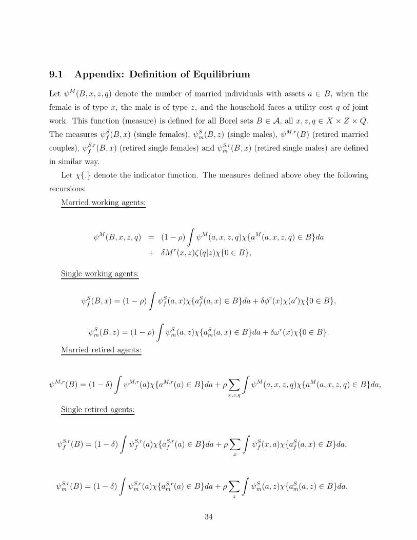
9.1 Appendix: Definition of Equilibrium

Let ψM(B, x, z, q) denote the number of married individuals with assets a ∈ B, when the

female is of type x, the male is of type z, and the household faces a utility cost q of joint

work. This function (measure) is defined for all Borel sets B ∈ A, all x, z, q ∈ X × Z × Q.

The measures ψSf (B, x) (single females), ψS

m(B, z) (single males), ψM,r(B) (retired married

couples), ψS,rf (B, x) (retired single females) and ψS,r

m (B, x) (retired single males) are defined

in similar way.

Let χ. denote the indicator function. The measures defined above obey the following

recursions:

Married working agents:

ψM(B, x, z, q) = (1 − ρ)

∫ψM(a, x, z, q)χaM(a, x, z, q) ∈ Bda

+ δM r(x, z)ζ(q|z)χ0 ∈ B,

Single working agents:

ψSf (B, x) = (1 − ρ)

∫ψS

f (a, x)χaSf (a, x) ∈ Bda+ δφr(x)χ(a′)χ0 ∈ B,

ψSm(B, z) = (1 − ρ)

∫ψS

m(a, z)χaSm(a, x) ∈ Bda+ δωr(x)χ0 ∈ B.

Married retired agents:

ψM,r(B) = (1 − δ)

∫ψM,r(a)χaM,r(a) ∈ Bda+ ρ

∑

x,z,q

∫ψM(a, x, z, q)χaM(a, x, z, q) ∈ Bda,

Single retired agents:

ψS,rf (B) = (1 − δ)

∫ψS,r

f (a)χaS,rf (a) ∈ Bda+ ρ

∑

x

∫ψS

f (x, a)χaSf (a, x) ∈ Bda,

ψS,rm (B) = (1 − δ)

∫ψS,r

m (a)χaS,rm (a) ∈ Bda+ ρ

∑

z

∫ψS

m(a, z)χaSm(a, z) ∈ Bda.

34

Equilibrium Definition: For a given government consumption level G, social security

tax benefits bM , bSf and bSm, tax functions T S(.), TM(.), a payroll tax rate τp, a capital

tax rate τk, and an exogenous demographic structure represented by Ω(z), Φ(x), M(x, z),

a stationary equilibrium consists of prices r and w, aggregate capital (K) and labor (L),

household decision rules lMf (a, x, z, q), lMm (a, x, z, q), lSm(a, z), lSf (a, x), aM(a, x, z, q), aSm(a, z),

aSf (a, x), aM,r(a), aS,r

m (a), and aS,rf (a), and measures ψM , ψS

f , ψSm, ψ

M,r, ψS,rf and ψS,r

m such

that

1. Given tax rules and factor prices, the decision rules of households are optimal.

2. Factor prices are competitively determined; i.e. w = F2(K,L), and r = F1(K,L)− δk.

3. Factor markets clear; i.e.,

K =∑

x, z, q

∫

A

aψM(a, x, z, q)da+∑

z

∫

A

aψSm(a, z)da+

∑

x

∫

A

aψSf (a, x)da

+

∫

A

aψM,r(a)da+

∫

A

aψS,rm (a)da+

∫

A

aψS,rf (a)da,

L =∑

x, z, q

∫

A

(xlMf (a, x, z, q) + zlMm (a, x, z, q))ψM(a, x, z, q)da+

∑

z

∫

A

zlSm(a, z)ψSm(a, z)da+

∑

x

∫

A

xlSf (a, x)ψSf (a, x)da.

4. The measures ψM , ψSf , ψS

m, ψM,r, ψS,r

f and ψS,rm are consistent with individual decisions.

5. The Government Budget and Social Security Budgets are Balanced; i.e.,

G =∑

x,z,q

∫

A

TM(.)ψM(a, x, z, q)da+∑

z

∫

A

T S(.)ψSm(a, z)da

+∑

x

∫

A

T S(.)ψSf (a, x)da+ τkK,

∫

A

bMψM,r(a)da+

∫

A

bSfψS,rf (a)da+

∫

A

bSmψS,rm (a)da = τ pwL

35

Table 1: Productivity Levels, by Type, by Gender

Males (z) Females (x) x/z<hs 0.709 0.505 0.712hs 0.920 0.669 0.727sc 1.113 0.799 0.718col 1.447 1.052 0.727>col 1.809 1.326 0.733

Note: Entries are the productivity levels of males and females, using 2000 data

from the Consumer Population Survey. These levels are constructed as hourly

wages for each type –see text for details.

Table 2: Distribution of Married Working Households by Type, %

FemaleMale <hs hs sc col >col<hs 6.76 4.24 2.32 0.39 0.17hs 3.15 13.49 7.29 1.83 0.68sc 1.75 7.44 13.51 4.32 1.56col 0.39 2.36 5.76 7.58 2.61>col 0.17 0.90 2.63 4.42 4.27

Note: Entries show the fractions of the total married pool, by wife and husband

educational categories. The data used is from the U.S. 2000 Census –see text for

details.

36

Table 3: Fraction of Agents By Type, By Gender, and Marital Status

Males FemalesAll Married Singles Singles (data) All Married Singles Singles (data)

<hs 0.1439 0.1028 0.0411 0.0386 0.1360 0.0904 0.0456 0.0403hs 0.2659 0.1958 0.0701 0.0703 0.2793 0.2105 0.0688 0.0679sc 0.2891 0.2115 0.0776 0.0773 0.3159 0.2331 0.0828 0.0848col 0.1858 0.1384 0.0474 0.0488 0.1760 0.1373 0.0387 0.0423>col 0.1153 0.0915 0.0238 0.0250 0.0928 0.0687 0.0241 0.0247

Total: 1.0000 0.74 0.26 0.26 1.0000 0.74 0.26 0.26

Note: Entries show the fraction of individuals in each educational category, by

marital status, constructed under the assumption of a stationary population

structure –see text for details. The last column in each panel shows the cor-

responding values in U.S. 2000 Census data.

Table 4: Tax Parametersη1 η2

Married 0.1023 0.0733R2 0.99

Single 0.1547 0.0497R2 0.93

Note: Entries show the parameter estimates for the postulated tax function.

These result from regressing effective average tax rates against household in-

come, using 2000 data from the U.S. Internal Revenue Service – see text for

details.

37

Table 5: Labor Force Participation of Married Females (%)

FemaleMale <hs hs sc col >col<hs 41.1 62.5 72.1 77.4 70.9hs 49.1 67.7 77.6 84.3 86.6sc 50.1 68.1 74.9 82.9 88.9col 49.5 64.4 68.8 73.4 83.7>col 45.8 58.4 62.8 64.1 79.1

Total 44.8 66.5 73.2 74.6 82.5

Note: Each entry shows the labor force participation of married females, calcu-

lated from 2000 data from the Consumer Population Survey –see text for details.

The outer row shows the weighted average for a fixed male or female type.

38

Table 6: Parameter ValuesParameter Value CommentsDiscount Factor (β) 0.973 Calibrated - matches K/YIntertemporal Elasticity (Labor Supply) (γ) 0.4 Literature estimates.Disutility of Market Work (B) 6 Calibrated - matches hours per workerCapital Share (α) 0.317 Calibrated - see text.Depreciation Rate (δk) 0.07 Calibrated - see text.Probability of Retirement 1/40 Calibrated - implies average

working life of 40 yearsMortality rate (δ) 0.0982 Calibrated - implies fraction

of retired people in data.Payroll Tax Rate (τp) 0.086 Calibrated - balances budgetCapital Income Tax Rate (τk) 0.124 Calibrated - Matches corporate tax

collectionsDistribution of utility costs ζ(.|z) – Gamma Distribution - matches

LFP by educationconditional on husband’s type

Table 7: Model and DataStatistic Data ModelCapital Output Ratio 2.325 2.321Labor Hours Per-Worker 0.408 0.408Participation rate of Married Females(%)

Less than High School 44.8 45.0High School 66.5 66.1Less than College 73.2 72.9College 74.6 77.5More than College 82.5 81.6

Total 68.9 69.2

Note: Entries summarizes the performance of the benchmark model in terms of

the stated targets.

39

Table 8: Proportional Taxes (% change)

Consumption IncomeTax Tax

Labor Force Participation 7.3 6.2Aggregate Hours 4.7 4.3Aggregate Hours (Married Females) 10.6 9.3Hours per worker (female) 2.6 2.3Hours per worker (male) 2.8 2.6Labor Input 4.2 3.8Capital/Output 15.0 4.5Aggregate Output 11.2 5.9Wage 6.5 2.0Tax rate (%) 17.8 12.7

NOTE: The results for a “consumption (income) tax” pertain to the replacement

of current income taxes by a proportional consumption (income) tax. The values

for ’Tax Rate’ correspond to the proportional rates that are necessary to achieve

budget balance.

40

Table 9: Progressive Taxes (% change)

Progressive Consumption Tax Separate Filing

High Exemption Low ExemptionLabor Force Participation 3.2 6.3 5.9Aggregate Hours 1.5 3.6 2.1Aggregate Hours (Married Females) 4.4 8.7 7.3Hours per worker (female) 0.3 1.5 0.8Hours per worker (male) 0.9 2.1 0.2Labor Input 1.5 3.2 1.6Capital/Output 14.4 14.2 2.1Aggregate Output 8.0 9.8 2.6Wage 6.3 6.3 0.9Tax Rate (%) 27.5 21.5 -1.5%

Note: Results in the first two columns pertain to the introduction of a progressive

consumption tax, which consists of an exemption level and a common tax rate

applied above this level. The ’high’ (’low’) exemption level corresponds to 1/3

(1/6) mean consumption for single individuals, and 1/2 (1/4) mean consumption

for married households in the benchmark economy. The last column shows the

effects of taxing individuals rather than households, as explained in the text. The

values for ’Tax Rate’ correspond to the proportional rates that are necessary to

achieve budget balance.

41

Table 10: Contribution of Married Females to Changes in Labor Supply (%)

Propor. Propor. Progr. Progr. SeparateCons. Inc. Cons. Cons. Filing

(high exemp.) (low exemp.)

Panel A: Total Changes

∆ in Married Female Hours(% of Total ∆ in Hours) 59.3 58.1 80.1 64.9 91.4

∆ in Married Female Labor(% of Total ∆ in Labor) 50.5 49.4 65.2 55.0 88.6

Panel B: Extensive Margin

∆ in Married Female Hours(% of Total ∆ in Hours) 51.5 49.6 71.0 56.8 82.0

∆ in Married Female Labor(% of Total ∆ in Labor) 42.7 40.7 55.4 46.7 77.0

Note: The entries show the contribution of changes in the labor supply of married

females relative to total changes in labor supply, both in terms of raw hours

changes as well as in terms of labor in efficiency units. The top panel shows the

contribution of total changes. The bottom panel shows only the contribution of

changes along the extensive margin.

Table 11: Changes in Labor Force Participation

Propor. Propor. Prog. Prog. SeparateFemale Type Cons. Inc. Cons. Cons. Filing

(high exemp.) (low exemp.)

<hs 22.5 20.0 0.9 18.7 19.8hs 9.1 6.3 6.1 7.6 6.9sc 5.4 6.1 2.6 5.3 4.7col 4.5 3.5 2.4 3.7 3.3>col 2.7 1.7 1.0 2.2 1.7

Note: The entries show the percentage changes in labor force participation, ar-

ranged by the female type, for all reforms considered.

42

Table 12: Reforms with Low Intertemporal Elasticity (% change)

Prop. Prop. Prog. Prog. SeperateCons. Inc. Cons. Cons. Filing

(high exemp.) (low exemp.)Labor Force Participation 11.0 8.9 5.0 8.4 5.5Aggregate Hours 4.6 3.9 1.7 3.4 1.8Aggregate Hours (Married Fem.) 13.0 10.7 5.8 9.9 6.2Hours per worker (female) 1.7 1.5 0.2 1.2 0.7Hours per worker (male) 1.4 1.2 0.2 0.9 0.0Labor Input 3.8 3.2 1.4 2.8 1.3Aggregate output 10.3 5.4 8.0 9.4 2.7

∆ in Married Female Hours(% of Total ∆ in Hours) 79.0 76.3 96.3 81.7 98.0∆ in Married Female Labor(% of Total ∆ in Labor) 71.2 68.4 86.2 73.6 96.0

Note: Results show the aggregate consequences of tax reforms under a low value

of the intertemporal elasticity parameter (γ = 0.2).

Table 13: Comparison with Standard Framework

High Elasticity (γ = 0.4) Low Elasticity (γ = 0.2)Current Standard Current Standard

Framework Framework Framework Framework

Aggregate Hours 4.7 3.4 4.6 1.9Labor Input 4.2 3.5 3.8 1.9Aggregate Output 11.2 10.0 10.3 8.8Hours per worker (male) 2.8 3.5 1.4 2.0

Note: The results show aggregate effects of a proportional consumption tax reform

under the framework developed in this paper, and under a version of a standard

macroeconomic model with a single earner as described in the text.

43

q*

q

V’1

V1

q*’ q

V’2V2

increase in labor force participation

Figure 1: Taxes and Labor Force Participation of Secondary Earners

44

FIG. 2: AVERAGE TAX RATES

-0.1

-0.05

0

0.05

0.1

0.15

0.2

0.25

0.3

0.1 0.5 0.9 1.3 1.7 2.1 2.5 2.9 3.3 3.7 4.1 4.5 4.9 5.3 5.7 6.1

INCOME/MEAN HOUSEHOLD INCOME

TA

X R

AT

E

Single Married

FIG. 3: MARGINAL TAX RATES

0

0.05

0.1

0.15

0.2

0.25

0.3

0.35

0.1 0.5 0.9 1.3 1.7 2.1 2.5 2.9 3.3 3.7 4.1 4.5 4.9 5.3 5.7 6.1

INCOME/MEAN HOUSEHOLD INCOME

MR

G.

TA

X R

AT

E

Single Married

45

References

[1] Albanesi, Stefania and C. Olivetti, “Gender Roles and Technological Progress” NBER

WP 13179 (June 2007).

[2] Altig, David, A. J. Auerbach, L. J. Kotlikoff, K. A. Smetters and J. Walliser, “Simulating

Fundamental Tax Reform in the United States,” American Economic Review, vol. 91,

no. 3, 574-595, June 2001.

[3] Attanasio, O., Low, H. and V. Sanchez Marcos, “Explaining Changes in Female Labor

Supply in a Life-Cycle Model,” Forthcoming in American Economic Review, 2007.

[4] Auerbach, Alan J. and Kevin A. Hassett, Toward Fundamental Tax Reform, The Amer-

ican Enterprise Institute Press, Washington, D.C. 2005.

[5] Blundell, R. and T. E. MaCurdy, “Labor Supply: a Review of Alternative Approaches,”

In Handbook of Labor Economics, vol. 3A, pages 1599-1695, ed. O. A Ashenfelter and

D. Card, Amsterdam: North Holland, 1999.

[6] Bosworth, B., and G. Burtless, “Effects of Tax Reform on Labor Supply, Investment,

and Savings,” Journal of Economic Perspectives, vol. 6, no. 1, (Winter 1992), 3-25.

[7] Castaneda, Ana, J. Dıaz-Gimenez and J. V, Rıos-Rull, “Accountig for the US Earnings

and Wealth Inequality”, Journal of Political Economy , 111, 4, August 2003, 818-857.

[8] Chade, Hector and G. Ventura, “Taxes and Marriage: A Two-Sided Search Analysis”,

International Economic Review, vol. 43, no. 3 (August 2002), 955-986.

[9] Chang, Yougsung and S. B. Kim. “From Individual to Aggregate Labor Supply: A

Quantitative Analysis based on a Heterogeneous-Agent Macroeconomy,” International

Economic Review, vol. 47, no. 1 (February 2006), 1-27.

[10] Cho, Jank-Ok., and R. Rogerson, “Family Labor Supply and Aggregate Fluctuations,”

Journal of Monetary Economics, vol. 21, no. 2, (March 1988), 233-245.

[11] Conesa, Juan Carlos and D. Krueger, “On the Optimal Progressivity of the Income Tax

Code,” Journal of Monetary Economics, vol. 53., no. 7, (October 2006), 1425-1450.

46

[12] Davis, Steven J., and M. Henrekson, “Tax Effects on Work Activity, Industry Mix

and Shadow Economy Size: Evidence From Rich Country Comparisons,” Manuscript,

University of Chicago Graduate School of Business, (2003).

[13] Diaz-Gimenez, Javier and Joseph Pijoan-Mas, “Flat Tax Reforms in the U.S.: A Boon

for the Income Poor,” mimeo, University of Carlos III, Madrid, Spain, 2005.

[14] Domeij, David and M. Floden, “The Labor-Supply Elasticity and Borrowing Con-

straints: Why Estimates are Biased”, Review of Economic Dynamics, vol. 9, no. 2

(April 2006), 242-262.

[15] Eissa, Nada, “Taxation and The Labor Supply of The Women: The Tax Reform Act of

1986 As A Natural Experiment,” NBER Working Paper, #5023, 1995.

[16] Eissa, Nada and H. W. Hoynes, “Behavioral Responses to Taxes: Lessons from the

EITC and Labor Supply,” Tax Policy and the Economy, vol. 20 (September 2006), pp.

74-110

[17] Erosa, Andres and Koreshkova, T., ”Progressive Taxation in a Dynastic Model of Hu-

man Capital”. Forthcoming in Journal of Monetary Economics, 2007.

[18] Fernandez, R., Guner, N. and John Knowles, “Love and Money: A Theoretical and Em-

pirical Analysis of Household Sorting and Inequality,” Quarterly Journal of Economics,

120, no 1 (February 2005), 273-344.

[19] Gertler, Mark, “Government Debt and Social Security in a Life-Cycle Economy,”

Carnegie-Rochester Conference on Public Policy, vol. 50 (1999), 61-110.

[20] Gouveia, M., and R. P. Strauss, “Effective Federal Individual Income Tax Functions:

An Exploratory Empirical Analysis,” National Tax Journal, vol. 40, no. 2, (June 1994),

317-339.

[21] Greenwood, Jeremy, and N. Guner, ”Marriage and Divorce since World War II: An-

alyzing the Role of Technological Progress on the Formation of Households,” NBER

Working Paper, # 10772, 2004.

47

[22] Guner, Nezih, G. Ventura and Y. Xu, ”Macroeconomic Implications of Size-Dependent

Policies,” CEPR Discussion Paper 6138, 2007.

[23] Hall, Robert E. and A. Rabushka, The Flat Tax, Stanford, CA: Hoover Institute Press,

1995.

[24] Heathcote, Jonathan, K. Storesletten, and G. L. Violante. “Consumption and Labor

Supply with Partial Insurance: An Analytical Framework,” mimeo, 2007.

[25] Hong, Jay and J. V. Rıos-Rull, “Social Security, Life Insurance and Annuities for Fam-

ilies”, 54(1), 118-140, Journal of Monetary Economics, 2007.

[26] Internal Revenue Service Statistic of Income Division, Individual Income Tax Returns,

1980, 1985, 1990, 1995 and 2000.

[27] Kaygusuz, Remzi. ”Taxes and Female Labor Supply,” Manuscript, The Pennsylvania

State University, 2006a.

[28] Kaygusuz, Remzi. ”Social Security and Two-Earner Households,” Manuscript, The

Pennsylvania State University, 2006b.

[29] Kleven, Henrik J. and C. T. Kreiner, “”The Efficient Taxation of Couples,” Manuscript,

University of Copenhagen, 2006.

[30] Knowles, John. “Why Are Married Men Working So Much?,” Manuscript, The Univer-

sity of Pennsylvania, 2007.

[31] Mulligan, Casey B., “Aggregate Implications of Indivisible Labor,” Advances in Macroe-

conomics, vol.1, no.1, (2001).

[32] Nishiyama, Shinichi and K. Smetters, “Consumption Taxes and Economic Efficiency

with Idiosyncratic Wage Shocks,” Journal of Political Economy, vol.113, no.5 (October

2005), pp.1088-1115.

[33] Olovsson, Conny,“Why Do Europeans Work So Little?,” Manuscript, Institute of Eco-

nomic Studies, Stockholm University, 2003.

48

[34] Prescott, Edward C., “Why Do Americans Work So Much More Than Europeans?,”

Federal Reserve Bank of Minneapolis Quarterly Review, (July 2004), 2-13.

[35] Rogerson, Richard “Understanding differences in hours worked,” Review of Economic

Dynamics, vol. 9, no. 3 (July 2006), 365-409.

[36] Triest, Robert K. “The Effects of Income Taxation on Labor Supply in the United

States,” Journal of Human Resources vol. 25, no. 3 (Summer 1990), 491-516.

[37] Ventura, Gustavo, ”Flat Tax Reform: A Quantitative Exploration,” Journal of Eco-

nomic Dynamics & Control, vol. 23, no. 9-10, (September 1999), 1425-1458.

49