Taxation and Household Labor Supply

Nezih Guner, Remzi Kaygusuz and Gustavo Ventura∗

July 2011

Abstract

We evaluate reforms to the U.S. tax system in a life-cycle setup with heterogeneousmarried and single households, and with an operative extensive margin in labor supply.We restrict our model with observations on gender and skill premia, labor force par-ticipation of married females across skill groups, children, and the structure of maritalsorting. We concentrate on two revenue-neutral tax reforms: a proportional incometax and a reform in which married individuals file taxes separately (separate filing).Our findings indicate that tax reforms are accompanied by large increases in labor sup-ply that differ across demographic groups, with the bulk of the increase coming frommarried females. Under a proportional income tax reform, married females accountfor more than 50% of the changes in hours across steady states, while under separatefiling reform, married females account for all the change in hours.

JEL Classifications: E62, H31, J12, J22Key Words: Taxation, Two-earner Households, Labor Force Participation.

∗Guner, ICREA-MOVE, Universitat Autonoma de Barcelona, Barcelona GSE; Kaygusuz, Faculty of Artsand Social Sciences, Sabanci University, Turkey; Ventura, Department of Economics, University of Iowa,USA. We thank the Editor, three referees, and participants NBER Summer Institute (Aggregate Implica-tions of Microeconomic Consumption Behavior, Macro Perspectives), Minnesota Macro Conference, SED,Midwest Macro Conference, LACEA Meetings, “Households, Gender and Fertility: Macroeconomic Perspec-tives” Conference in UC-Santa Barbara, “Research on Money and Markets” Conference, ESOP Workshopon Gender and Households, Public Economic Theory Conference, European University Institute, FederalReserve Banks of Minneapolis and Richmond, Arizona State, Bilkent, Cornell, IIES, IZA, Illinois, Indiana,Purdue, Sabanci, Toulouse, and Wisconsin for helpful comments. We thank the Population Research Insti-tute at Pennsylvania State for support. Guner thanks Instituto de Estudios Fiscales (Ministerio de Economiay Hacienda), Spain, Ministerio de Educacion y Ciencia, Spain, Grant SEJ2007-65169, and Fundacion RamonAreces for support. Earlier versions of this paper circulated under the title “Taxation, Aggregates and theHousehold.” The usual disclaimer applies.

1

1 Introduction

Tax reforms have been at the center of numerous debates among academic economists and

policy makers. As a part of this debate, there have been calls for tax reforms that would

simplify the tax code, change the tax base from income to consumption, and adopt a more

uniform marginal tax rate structure.1

In the existing literature, the decision maker is typically an individual who decides how

much to work, how much to save, and in some cases how much human capital investments

to make. Yet, current households are neither a collection of bread-winner husbands and

house-maker wives, nor a collection of single people. In 2000, the labor force participation

of married women between ages 25 and 54 was about 69%. Furthermore, their participation

rate increases markedly by educational attainment, and is known to respond strongly to

hourly wages. Moreover, the economic environment that these households face does not

feature wages that are gender-neutral. Hourly earnings of females relative to males, the

gender-gap, is of about 70% nowadays and has been around this value for some time.2

These observations have long been deemed important in discussions of tax reforms, but

are largely unexplored in dynamic equilibrium analyses in the macroeconomic and public-

finance literatures. We fill this void in this paper. We quantify the effects of tax reforms

taking carefully into account the labor supply of married females as well as the current

demographic structure. For these purposes, we develop a dynamic equilibrium model with

an operative extensive margin in labor supply, and a structure of individual and household

heterogeneity that is consistent with the current U.S. demographics.

We consider a life-cycle economy populated with males and females who differ in their

labor market productivities. Individuals start economic life as eithermarried or single and do

not change their marital status as they age. Married couples and single females have children

that appear exogenously along their life-cycle; they can be childless or have these children

early or late in their life-cycle. Singles decide how much to work and how much to save out of

their total after-tax income. Married households decide on the labor hours of each household

member, and like singles, how much to save. A novel feature in our analysis is the explicit

modeling of the participation decision of married females in two-earner households and its

interplay with the structure of heterogeneity and taxation. In the model, female labor-force

participation is not a trivial decision for a household. First, children are associated to fixed

time costs. Furthermore, if a female with a child decides to work, the household incurs

1See Auerbach and Hassett (2005) for a review.2Our calculations. See Section 4.1 for details.

2

child care expenses. Second, her labor market productivity depreciates if she chooses not to

participate. Finally, if a married female enters the labor force, the household faces a utility

cost. This cost allows us to capture residual heterogeneity in labor force participation.

It represents heterogeneity in the additional difficulty of coordinating multiple household

activities, taste for children and home production or any other utility cost that might arise

when two adults work instead of one. As a result of these assumptions, females in married

households may choose not to work at all. This is a key feature of our analysis since the

structure of taxation can affect the participation decision of married females, and available

evidence suggests that it does so significantly.

There are several reasons that point to the relevance of our analysis. First, in the current

U.S. tax system the household (not the individual) constitutes the basic unit of taxation,

which results in high tax rates on secondary earners. When a married female considers

entering the labor market, the first dollar of her earned income is taxed at her husband’s

current marginal rate. Second, from a conceptual standpoint, wages of each member as well

as the presence of children in a two-earner household affect joint labor supply decisions as

well as the reactions to changes in the tax structure. Finally, a common view among many

economists has been that tax changes may have moderate impacts on labor supply. This

view is supported by empirical findings on the low or near zero labor supply elasticities of

prime-age males. Recent developments, however, started to challenge this wisdom. Tax

reforms in the 1980’s have been shown to affect female labor supply behavior significantly,

but have relatively small effects on males (Bosworth and Burtless (1992), Triest (1990), and

Eissa (1995)).3 These findings are consistent with ample empirical evidence that female labor

supply in general, and female labor force participation in particular are quite elastic (Blundell

and MaCurdy (1999), Keane (2010)). If households, not individuals, react to taxes much

more than previously thought, the potential effects of tax reforms can be more significant.

We use our framework to conduct two hypothetical tax reform experiments, and then

ask: What is the importance of the labor supply responses of married females in these

experiments? What is the importance of micro, labor-supply elasticities for the long-run

effects on output and the labor input?

We concentrate on two revenue-neutral tax reforms. The first one eliminates all pro-

gressivity via a proportional income tax. This is a prototypical reform, which allows us to

highlight and quantify the forces at work within the model. In our second reform, separate

3More recently, Eissa and Hoynes (2006) show that the disincentives to work embedded in the EarnedIncome Tax Credit (EITC) for married women are quite significant (effectively subsidizing some marriedwomen to stay at home).

3

filing, we keep the progressivity and the tax base of the current system, but married individ-

uals file their taxes separately. This reform, which arises naturally in our environment, shifts

the unit of taxation from households to individuals. As a result, it can drastically change

marginal tax rates within married households, while effectively eliminating tax penalties

(and bonuses) associated to marital status built into the current tax code.

A central finding of our exercises is that the differential labor supply behavior of different

groups is key for an understanding of the aggregate effects of tax reforms. The related finding

is that married females account for a disproportionate fraction of the changes in hours and

labor supply. Furthermore, the relative importance of the labor supply responses of married

females increases sharply for low values of the intertemporal elasticity of labor supply.

Replacing current income taxes by a proportional tax increases aggregate output by

about 7.4% across steady states. This increase is accompanied by differential effects on

labor supply: while hours per worker increase by about 3.3%, the labor force participation

of married females increases by about 4.6% and married females increase their total hours by

8.8%, with a significant response in the participation rate of married females with children

which increases by 6.8%.

Our results show that separate filing goes a long way in generating significant aggregate

output effects. With separate filing, aggregate output goes up by nearly 4%, which is more

than half of the increase from a proportional income tax reform. The increase in aggregate

output mainly comes from the rise in aggregate hours by married females. The labor force

participation of married females rises more than twice as it does under a proportional income

tax reform: an increase of 10.4% versus 4.6%. The rise in labor force participation of married

females with children is even stronger, increasing by about 18.1% with separate filing. In

contrast, male hours per worker remains nearly constant across steady states.

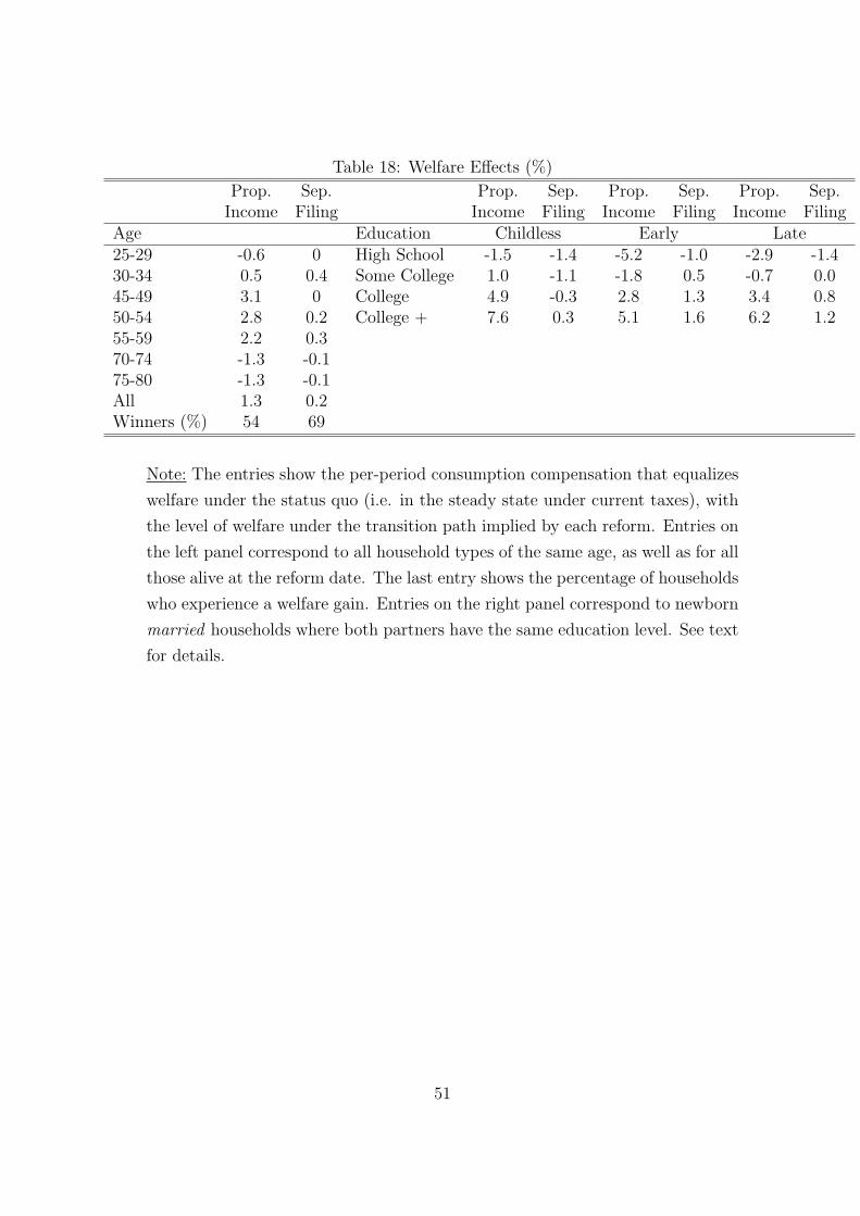
We find that both reforms lead to aggregate welfare gains for the generations that are

alive at the time of reforms. The welfare gains are larger under a proportional income

tax than under separate filing; the consumption compensation amounts to 1.3% under a

proportional income tax and 0.2% under the separate filing case. We also find that a

majority of households that alive at the time of reforms benefit from them. More households

benefit from a move to separate filing (about 69%) than under a proportional tax (54%).

In answering the first question posed above, “what is the importance of the labor supply

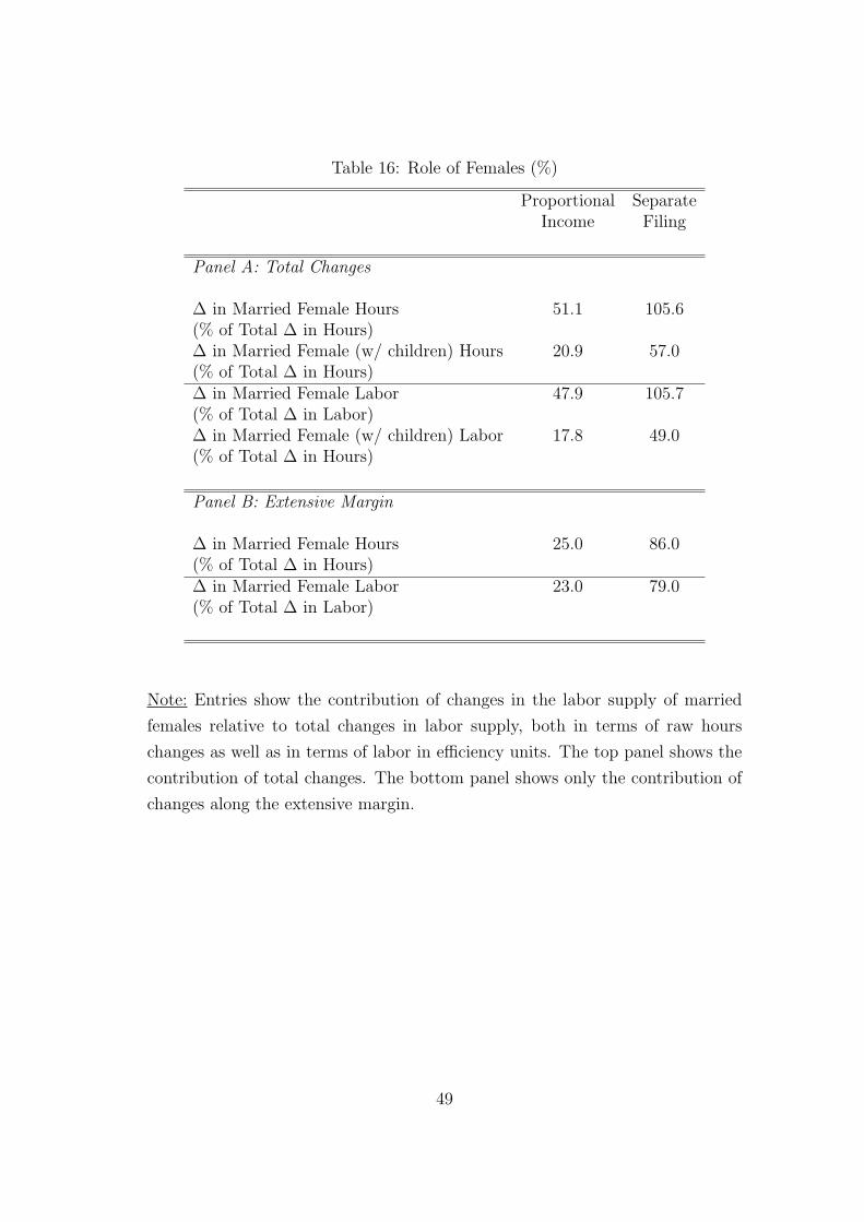
responses of married females in these experiments?”, we find that married females account

for a disproportionate fraction of the changes in hours and labor supply. Under proportional

taxes, married females account for about 51% of the total increase in labor hours, and about

48% of the aggregate increase in labor supply (efficiency units). With separate filing almost

4

all of the rise in hours and labor supply comes from married females. Hence, considering

explicitly the behavior of this group is key in assessing the effects of tax reforms on labor

supply.

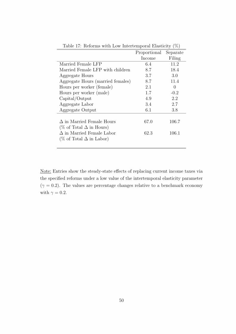
In answering the second question, “what is the importance of micro, labor-supply elas-

ticities for the long-run effects on output and the labor input?”, we find that when reducing

the intertemporal elasticity from the benchmark value of 0.4 to 0.2, the long-run response

of aggregate hours and output to tax changes is not critically affected. This occurs as while

households react much less to tax changes along the intensive margin under a low elasticity

parameter, they respond disproportionately via changes in labor force participation. Then,

a central finding is that the value of this preference parameter is of second-order importance

in assessing the effects on labor supply associated to tax reforms.

Related Literature Our work largely builds on two main strands of literature. First,

our evaluation of tax reforms using a dynamic model with heterogeneity follows the work

by Ventura (1999), Altig, Auerbach, Kotlikoff, Smetters and Walliser (2001), Castaneda,

Dıaz-Jimenez and Rıos-Rull (2003), Dıaz-Jimenez and Pijoan-Mas (2005), Nishiyama and

Smetters (2005), Conesa and Krueger (2006), Erosa and Koreshkova (2007), and Conesa,

Kitao and Krueger (2009), among others. In contrast to these papers, we study economies

populated with married and single households, where married households can have one or two

earners. In this vein, Kaygusuz (2010) studies the effects of the 1980s tax reforms on female

labor force participation in the U.S. Hong and Rıos-Rull (2007) and Kaygusuz (2006) study

social security in environments with an explicit role for two-member households. Chade and

Ventura (2002) study the effects of tax reforms on labor supply and assortative matching in

a model with heterogenous individuals and endogenous marriage decisions. They abstract,

however, from the extensive margin in labor supply, among other things. Alesina, Ichino and

Karabarbounis (2009) study the Ramsey optimal taxation problem of a two-earner household

within a static environment, where lower tax rates for females emerge. Kleven, Kreiner and

Saez (2009) study a similar optimal taxation of problem in Mirrlessian framework, where

second earner makes an explicit labor force participation decision. Second, as Cho and

Rogerson (1988), Mulligan (2001), and Chang and Kim (2006), we study the aggregate

effects of changes in labor supply along the extensive margin. As Rogerson and Wallenius

(2009), we differ from these papers by explicitly analyzing the role of the extensive margin

for public policy.

Our paper is also related to two recent literatures. First, it is related to recent work that

argues that the structure of taxation can significantly affect labor choices, and play a central

5

role in accounting for cross-country differences in labor supply behavior. Prescott (2004),

Rogerson (2006), Ohanian, Raffo and Rogerson (2008), and Olovsson (2009) are examples of

papers in this group. Our paper is also related to recent work that studies female labor supply

in macroeconomic setups; Jones, Manuelli and McGrattan (2004), Greenwood, Seshadri and

Yorukoglu (2005), Erosa, Fuster, Restuccia (2010), Albanesi and Olivetti (2007), Knowles

(2007), Attanasio, Low and Sanchez Marcos (2008), and Greenwood and Guner (2009) are

representative papers in this group.

The paper is organized as follows. Section 2 presents an example that highlights the role

of taxation with two-earner households, and motivates the parameterization of the model

economy. Section 3 presents the model economy. Section 4 discusses the parameterization

of the model and the mapping to data. Results from tax reforms are presented in section

5. Section 6 quantifies the role of married females and the extensive margin in labor supply.

Section 7 discusses the implications of a lower labor supply elasticity. Section 8 presents

some welfare results. Section 9 concludes.

2 Taxation, Two-Earner Households and the Extensive

Margin

In this section, we present a simple static, decision-problem that illustrates how taxes affect

labor supply decisions with two-earner households with and without children, with an em-

phasis on the potential changes in labor force participation. The example serves to highlight

key features of our general environment, and to understand some of the calibration choices

we make later.

Consider a married household. The household decides whether only one or both members

should work and if so, how much. Let x and z denote the labor market productivities (wage

rates) of males and females, respectively. Let τ be a proportional tax on labor income. The

household can be childless (k = 0) or have children (k = 1). Couples with children have to

pay for child care services only if both household members works. Taking care of children

costs d > 0 units of consumption.

A one-earner household Consider first the problem if only one member (husband)

works. For couples with and without children, the household problem is given by

maxlm,1

2[log((1− τ)zlm,1 + T )︸ ︷︷ ︸=log(c)

]− φl1+ 1

γ

m,1 ,

6

where lm,1 is the labor choice of the primary earner (husband) and T is a transfer received

from the government. The subscript 1 represents the choices of a one-earner household. The

function W ≡ φl1+1γ stands for the disutility associated to work time.

We introduce government transfers in order to capture in a simple way the role of pro-

gressive taxation. This follows as household choices under non-linear, progressive taxes are

qualitatively equivalent to choices under a linear tax system that combines a proportional

tax rate plus a lump-sum transfer. Under a progressive tax system, changes in marginal

tax rates affect labor choices even for preferences for which income and substitution effects

cancel out; the same occurs under the linear tax system that we consider.

Household utility when only one member works is given by

V1(τ) = 2[log((1− τ)zl∗m,1 + T )]−W (l∗m,1),

where a ′∗′ denotes an optimal choice.

A two-earner household When both members work, the household incurs a utility

cost q, drawn from a distribution with cumulative distribution function ζ(q). Then the

problem is given by

maxlm,2,lf,2

2[log((1− τ)(zlm,2 + xlf,2) + T − dχ(k))︸ ︷︷ ︸=log(c)

]

−φl1+ 1

γ

m,2 − φl1+ 1

γ

f,2 − q,

where χ(k) is an indicator for the presence of children, and the subscript 2 represents the

choices of a two-earner household. Let the solutions to this problem be denoted by l∗m,2(k = 0)

and l∗f,2(k = 0). Similarly, let l∗m,2(k = 1) and l∗f,2(k = 1) be the optimal decisions when

children are present. Household utility levels are given by

V2(τ , k)− q = 2[log((1− τ)(zl∗m,2(k) + xl∗f,2(k)) + T − dχ(k))]

−W (l∗m,2(k))−W (l∗f,2(k))− q,

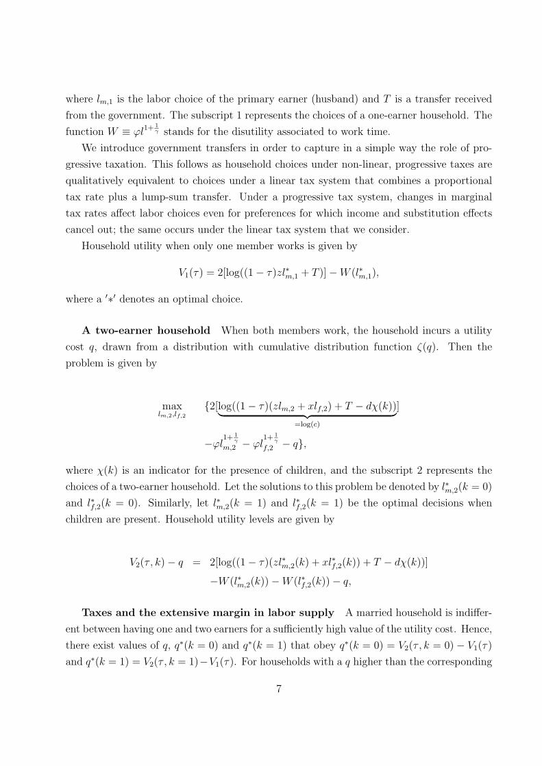
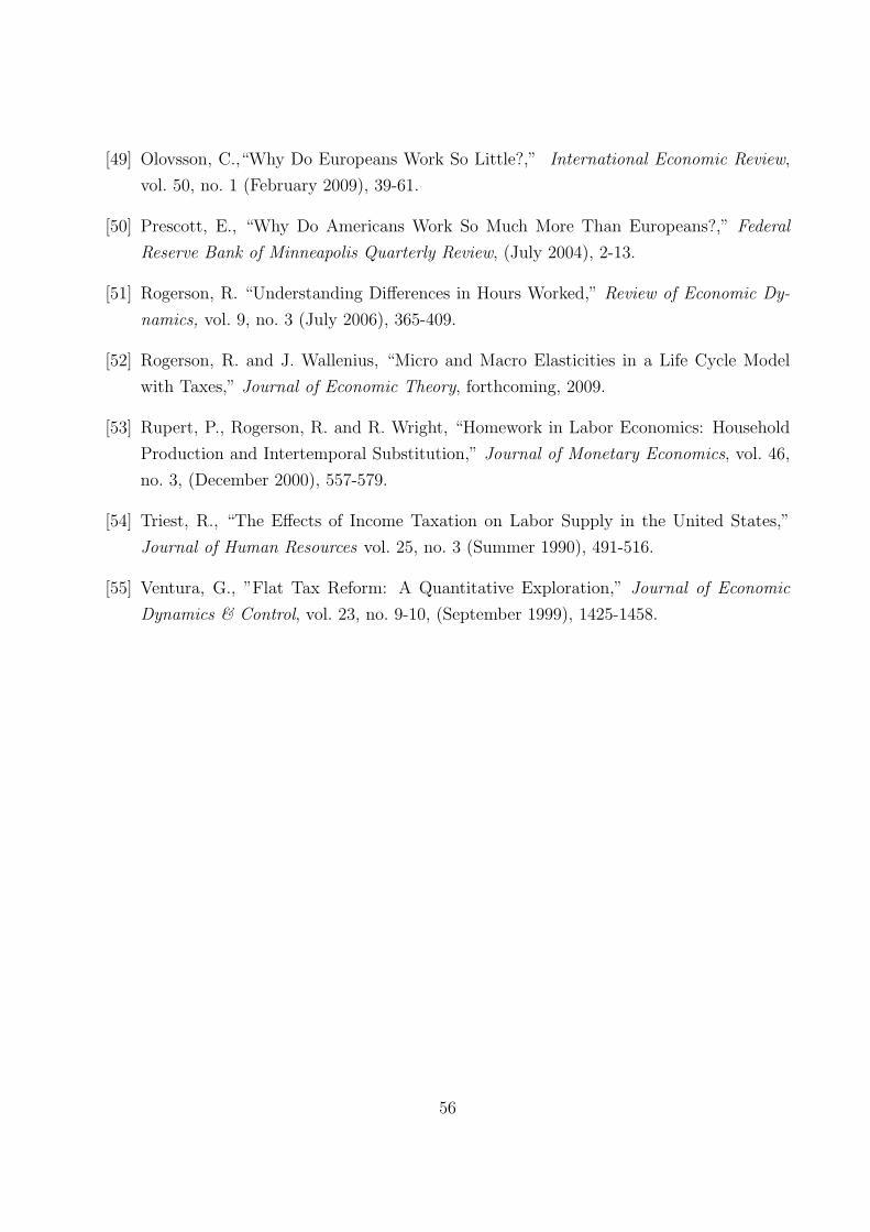
Taxes and the extensive margin in labor supply A married household is indiffer-

ent between having one and two earners for a sufficiently high value of the utility cost. Hence,

there exist values of q, q∗(k = 0) and q∗(k = 1) that obey q∗(k = 0) = V2(τ , k = 0)− V1(τ)

and q∗(k = 1) = V2(τ , k = 1)−V1(τ). For households with a q higher than the corresponding

7

threshold value, it is optimal to have only one earner, while for those with a q lower than

the threshold it is optimal to be a two-earner household. Since children are costly, it follows

that q∗(k = 0) > q∗(k = 1). Hence, everything else the same, childless couples are more

likely to have two members working in the market than couples with children.

Thresholds will change as taxes change. Using the envelope theorem, it follows that

∂q∗(k)

∂τ=∂V2(τ , k)

∂τ− ∂V1(τ)

∂τ< 0,

This derivative is negative if household consumption with two earners is higher than

with one earner, a condition that necessarily holds in our case.4 That is, q∗(k = 0) and

as a result, the labor force participation of married females without children, will be lower

(higher) when taxes are high (low) if the above condition holds. This is illustrated in Figure

1. Thus, a change in tax rates affects also the extensive margin in labor supply. For couples

with children, a similar result can be shown.

Furthermore, since children are costly in terms of resources, it is possible to show that

|∂q∗(k = 1)

∂τ| > |∂q

∗(k = 0)

∂τ|.

Hence, the participation response of married couples with children to tax changes is larger

than for couples without children.5

This example has important implications for the mapping of our model economy to the

data. On the one hand, the relative size of households with and without children affects the

size of labor supply response. On the other hand, as the bottom panel of Figure 1 shows,

exactly how much the labor force participation of married females will increase depends

on the shape of ζ(q). Therefore, selecting the functional form for the distribution of utility

costs will be an important part of the model parameterization; the magnitude of the response

along the extensive margin depends on slope ζ ′(q). We capture this slope by exploiting the

observed differences in female labor force participation in response to changes in the gender

gap, x/z. The key to this procedure is that an increase in x, for a given z, implies an increase

in labor force participation whose magnitude hinges precisely on the magnitude of ζ ′(q).

4This follows from the fact that income effects from female labor supply imply that males work less whenthey are in a two-earner household, i.e. l∗m,2 < l∗m,1. Since the first-order condition for husband’s hoursimplies that marginal disutility from work has to be equal to the marginal utility from consumption timesthe after-tax wage rate, household consumption with two earners must be higher than with one earner.

5For this inequality to hold household consumption with two earners must be lower with children thanwithout children, which follows naturally from the negative income effect of children on labor supply decisions.

8

3 The Economic Environment

We study a stationary overlapping generations economy populated by a continuum of males

(m) and a continuum of females (f). Let j ∈ 1, 2, ..., J denote the age of each individual.

Population grows at rate n. For tractability, individuals differ in terms of their marital status:

they are born as either single or married, and their marital status does not change over time.

Married households and single females also differ in terms of the number of children

attached to them. Married households and single females can be childless or endowed with

two children. These children appear either early or late in the life-cycle exogenously, and

affect the resources available to households for three periods. Children do not provide any

utility.

The life-cycle of agents is split into two parts. Each agent starts life as a worker and at

age JR, individuals retire and collect pension benefits until they die at age J. We assume

that married households are comprised by individuals who are of the same age. As a result,

members of a married household experience identical life-cycle dynamics.

Each period, working households (married or single) make labor supply, consumption and

savings decisions. Children imply a fixed time cost for females. If a female with children,

married or single, works, then the household also has to pay child care costs. Not working

for a female is costly ; if she does not work, she experiences losses of labor efficiency units for

next period. Furthermore, if the female member of a married household supplies positive

amounts of market work, then the household incurs a utility cost.

Heterogeneity and Demographics Individuals differ in terms of their labor effi-

ciency units. At the start of life, each male is endowed with an exogenous type z, where

z ∈ Z and Z ⊂ R++ is a finite set. The type of a male agent remains constant over his life

cycle. Let the age-j productivity of a type-z agent be denoted by the function ϖm(z, j). Let

Ωj(z) denote the fraction of age-j, type-z males in male population, with∑

z∈Z Ωj(z) = 1.

Each female starts her working life with a particular intrinsic type. As males, this type

is fixed over time and is denoted by x ∈ X, where X ⊂ R++ is a finite set. Let Φj(x) denote

the fractions of age-j, type-x females in female population, with∑

x∈X Φj(x) = 1.

As women enter and leave the labor market, their labor market productivity levels evolve

endogenously. Each female starts life with an initial productivity level that depends on

her intrinsic type, h1 = η(x) ∈ H. The next period’s productivity level (h′) depends on

the female’s intrinsic type x, her age, the current level of h and current labor supply (l).

Formally, for j ≥ 1,

9

h′ = G(x, h, l, j)

all h ∈ H. The function G is increasing in h and x and non-decreasing in l. It captures

the combined effects of a female intrinsic type, age and labor supply decisions on her labor

market productivity growth. We specify this function in detail in section (4).

Let Mj(x, z) denote the fraction of marriages between an age-j, type-x female and an

age-j type-z male, and let ωj(z) and ϕj(x) be the fraction of single type-z males and the

fraction of single type-x females, respectively. Then, the following accounting identity must

hold

Ωj(z) =∑x∈X

Mj(x, z) + ωj(z). (1)

Furthermore, since the marital status does not change,Mj(x, z) =M(x, z) and ωj(z) = ω(z)

for all j, which implies Ωj(z) = Ω(z). Similarly, for age-j females, we have

Φj(x) =∑z∈Z

Mj(x, z) + ϕj(x). (2)

Since marital status does not change ϕj(x) = ϕ(x) and Φj(x) = Φ(x) for all j

We assume that each cohort is 1 + n bigger than the previous one. These demographic

patterns are stationary so that age j agents are a fraction µj of the population at any point in

time. The weights are normalized to add up to one, and obey the recursion, µj+1 = µj/(1+n).

Children Children are assigned exogenously to married couples and single females at

the start of life, depending on the intrinsic type of parents. Each married couple and single

female can be of three types: early child bearers, late child bearers, and those without any

children. Early and late child bearers have two children for three periods. Early child bearers

have these children in ages j = 1, 2, 3 while late child bearers have children attached to them

in ages j = 2, 3, 4.

Child Care Costs We assume that if a female with children works, married or single,

then the household has to pay for child care costs. Child care costs depend on the age of the

child (s). For a female with children of age s ∈ 1, 2, 3, the household needs to purchase

d(s) units of (child care) labor services for their two children. Since the competitive price of

child care services is the wage rate w, the total cost of child care services for two children

equals wd(s).

10

Utility Cost of Joint Work We assume that at the start of their lives married house-

holds draw a q ∈ Q, where Q ⊂ R++ is a finite set. These values of q represent the utility

costs of joint market work for married couples. For a given household, the initial draw of a

utility cost depends on the intrinsic type of the husband. Let ζ(q|z) denote the probability

that the cost of joint work is q, with∑

q∈Q ζ(q|z) = 1.

Preferences The momentary utility function for a single female is given by

USf (c, l, ky) = log(c)− φ(l + kyκ)1+

1γ ,

where c is consumption, l is time devoted to market work, φ is a parameter controlling the

disutility of work, κ is fixed time cost having two age-1 (young) children for a female, and

γ is the intertemporal elasticity of labor supply. Here ky = 0 stands for the absence of age-1

(young) children in the household, whereas ky = 1 stands for young children being present.

Since a single male does not have any children, his utility function is simply given by

USm (c, l) = log(c)− φ(l)1+

1γ .

Married households maximize the sum of their members utilities. We assume that when

the female member of a married household works, the household incurs a utility cost q. Then,

the utility function for a married female is given by

UMf (c, lf , q, ky) = log(c)− φ(lf + kyκ)1+

1γ − 1

2χlfq,

while the one for a married male reads as

UMm (c, lm, lf , q) = log(c)− φl

1+ 1γ

m − 1

2χlfq,

where χ. denote the indicator function. Note that consumption is a public good within the

household. Note also that the parameter γ > 0, the intertemporal elasticity of labor supply,

and φ, the weight on disutility of work, are independent of gender and marital status.

Production and Markets There is an aggregate firm that operates a constant returns

to scale technology. The firm rents capital and labor services from households at the rate R

and w, respectively. UsingK units of capital and Lg units of labor, firms produce F (K,Lg) =

KαL1−αg units of consumption (investment) goods. We assume that capital depreciates at

rate δk. Households save in the form of a risk-free asset that pays the competitive rate of

return r = R− δk.

11

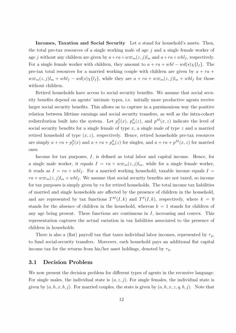
Incomes, Taxation and Social Security Let a stand for household’s assets. Then,

the total pre-tax resources of a single working male of age j and a single female worker of

age j without any children are given by a+ra+wϖm(z, j)lm and a+ra+whlf , respectively.

For a single female worker with children, they amount to a + ra + whl − wd(s)χlf. The

pre-tax total resources for a married working couple with children are given by a + ra +

wϖm(z, j)lm + whlf − wd(s)χlf, while they are a + ra + wϖm(z, j)lm + whlf for those

without children.

Retired households have access to social security benefits. We assume that social secu-

rity benefits depend on agents’ intrinsic types, i.e. initially more productive agents receive

larger social security benefits. This allows us to capture in a parsimonious way the positive

relation between lifetime earnings and social security transfers, as well as the intra-cohort

redistribution built into the system. Let pSf (x), pSm(z), and pM(x, z) indicate the level of

social security benefits for a single female of type x, a single male of type z and a married

retired household of type (x, z), respectively. Hence, retired households pre-tax resources

are simply a+ ra+ pSf (x) and a+ ra+ pSm(z) for singles, and a+ ra+ pM(x, z) for married

ones.

Income for tax purposes, I, is defined as total labor and capital income. Hence, for

a single male worker, it equals I = ra + wϖm(z, j)lm, while for a single female worker,

it reads as I = ra + whlf . For a married working household, taxable income equals I =

ra+ wϖm(z, j)lm + whlf . We assume that social security benefits are not taxed, so income

for tax purposes is simply given by ra for retired households. The total income tax liabilities

of married and single households are affected by the presence of children in the household,

and are represented by tax functions TM(I, k) and T S(I, k), respectively, where k = 0

stands for the absence of children in the household, whereas k = 1 stands for children of

any age being present. These functions are continuous in I, increasing and convex. This

representation captures the actual variation in tax liabilities associated to the presence of

children in households.

There is also a (flat) payroll tax that taxes individual labor incomes, represented by τ p,

to fund social-security transfers. Moreover, each household pays an additional flat capital

income tax for the returns from his/her asset holdings, denoted by τ k.

3.1 Decision Problem

We now present the decision problem for different types of agents in the recursive language.

For single males, the individual state is (a, z, j). For single females, the individual state is

given by (a, h, x, b, j). For married couples, the state is given by (a, h, x, z, q, b, j). Note that

12

the dependency of taxes on the presence of children in the household (k) is summarized by

age (j) and childbearing status (b): (i) k = 1 if b = 1, 2 and j = b, b+ 1, b+ 2, and (ii)

k = 0 if b = 2 and j = 1, or b = 1, 2 for all j > b + 2, or b = 0 for all j. Similarly, the

presence of age-1 (young) children (ky) depends on b and j.

The Problem of a Single Male Household Consider now the problem of a single

male worker of type (a, z, j). A single worker of type-(a, z, j) decides how much to work and

how much to save. His problem is given by

V Sm(a, z, j) = max

a′,lUS

m(c, l) + βV Sm(a′, z, j + 1) (3)

subject to

c+a′ =

a(1 + r(1− τ k)) + wϖm(z, j)l(1− τ p)− T S(wϖm(z, j)(j)l + ra, 0) if j < JR

a(1 + r(1− τ k)) + pSm(z)− T S(ra), otherwise,

and

l ≥ 0, a′ ≥ 0 (with strict equality if j = J)

The Problem of a Single Female Household In contrast to a single male, a single

female’s decisions also depends on her current human capital h and her child bearing status

b. Hence, given her current state, (a, x, h, b, j), the problem of a single female is

V Sf (a, h, x, b, j) = max

a′,lUS

f (c, l, ky) + βV Sf (a′, h′, x, b, j + 1),

subject to

(i) With kids: if b = 1, 2, j ∈ b, b+ 1, b+ 2, then k = 1, and

c+ a′ = a(1 + r(1− τ k)) + whl(1− τ p)− T S(whl + ra, 1)− wd(j + 1− b)χ(l).

Furthermore, if b = j , then ky = 1.

(ii) Without kids but not retired: if b = 0, or b = 1, 2 and b + 2 < j < JR, or b = 2 and

j = 1, then k = 0 and

c+ a′ = a(1 + r(1− τ k)) + whl(1− τ p)− T S(whl + ra, 0)

(ii) Retired: if j ≥ JR, k = 0 and

13

c+ a′ = a(1 + r(1− τ k)) + pSf (x)− T S(ra, 0).

In addition,

h′ = G(x, h, l, j),

l ≥ 0, a′ ≥ 0 (with strict equality if j = J)

Note how the cost of children depends on the age of children. If b = 1, the household has

children at ages 1, 2 and 3, then wd(j+1−b) denote cost for ages 1, 2 and 3 with j = 1, 2, 3.If b = 2, the household has children at ages 2, 3 and 4, then wd(j + 1− b) denotes the cost

for children of ages 1, 2 and 3 with j = 2, 3, 4. A female only incurs the time cost of

children if her kids are 1 year old, and this happens if b = j = 1 or b = j = 2.

The Problem of Married Households Like singles, married couples decide how

much to consume, how much to save, and how much to work. They also decide whether the

female member of the household should work. Their problem is given by

V M(a, h, x, z, q, b, j) = maxa′, lf , lm

[UMf (c, lf , q, ky) + UM

m (c, lm, lf , q)]

+ βV M(a′, h′, x, z, q, b, j + 1),

subject to

(i) With kids: if b = 1, 2, j ∈ b, b+ 1, b+ 2, then k = 1 and

c+ a′ = a(1 + r(1− τ k)) + w(ϖm(z, j)lm + hlf )(1− τ p)

− TM(wϖm(z, j)lm + whlf + ra, 1)− wd(j + 1− b)χ(lf )

Furthermore, if b = j , then ky = 1.

(ii) Without kids but not retired: if b = 0, or b = 1, 2 and b + 2 < j < JR, or b = 2,

j = 1, then k = 0 and

c+ a′ = a(1 + r(1− τ k)) + w(ϖm(z, j)lm + hlf )(1− τ p)

− TM(wϖm(z, j)lm + whlf + ra, 0)

(ii) Retired: if j ≥ JR, then k = 0 and

14

c+ a′ = a(1 + r(1− τ k)) + pM(x, z)− TM(ra, 0).

In addition,

h′ = G(x, h, lf , j)

lm ≥ 0, lf ≥ 0, a′ ≥ 0 (with strict equality if j = J)

3.2 Stationary Equilibrium

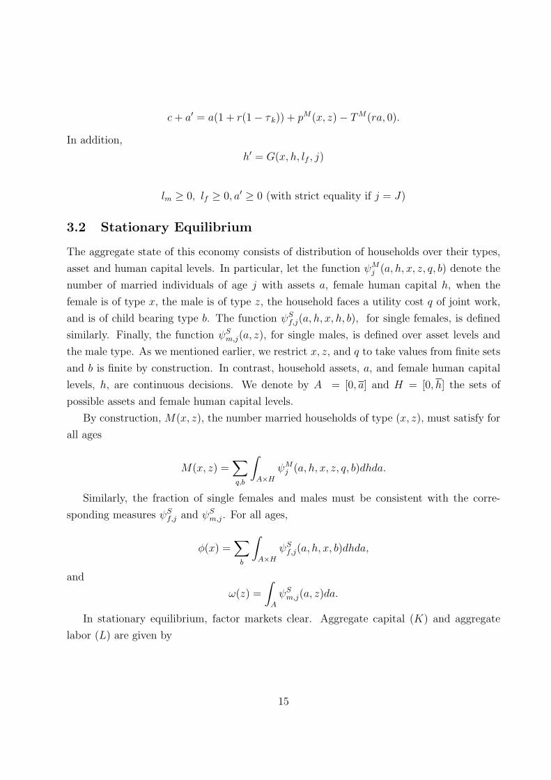
The aggregate state of this economy consists of distribution of households over their types,

asset and human capital levels. In particular, let the function ψMj (a, h, x, z, q, b) denote the

number of married individuals of age j with assets a, female human capital h, when the

female is of type x, the male is of type z, the household faces a utility cost q of joint work,

and is of child bearing type b. The function ψSf,j(a, h, x, h, b), for single females, is defined

similarly. Finally, the function ψSm,j(a, z), for single males, is defined over asset levels and

the male type. As we mentioned earlier, we restrict x, z, and q to take values from finite sets

and b is finite by construction. In contrast, household assets, a, and female human capital

levels, h, are continuous decisions. We denote by A = [0, a] and H = [0, h] the sets of

possible assets and female human capital levels.

By construction, M(x, z), the number married households of type (x, z), must satisfy for

all ages

M(x, z) =∑q,b

∫A×H

ψMj (a, h, x, z, q, b)dhda.

Similarly, the fraction of single females and males must be consistent with the corre-

sponding measures ψSf,j and ψ

Sm,j. For all ages,

ϕ(x) =∑b

∫A×H

ψSf,j(a, h, x, b)dhda,

and

ω(z) =

∫A

ψSm,j(a, z)da.

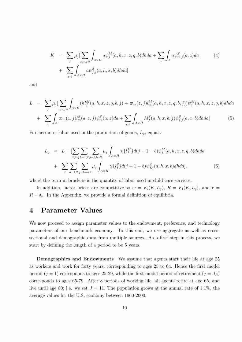
In stationary equilibrium, factor markets clear. Aggregate capital (K) and aggregate

labor (L) are given by

15

K =∑j

µj[∑x,z,q,b

∫A×H

aψMj (a, h, x, z, q, b)dhda+

∑z

∫A

aψSm,j(a, z)da (4)

+∑x,b

∫A×H

aψSf,j(a, h, x, b)dhda]

and

L =∑j

µj[∑x,z,q,b

∫A×H

(hlMf (a, h, x, z, q, b, j) +ϖm(z, j)lMm (a, h, x, z, q, b, j))ψM

j (a, h, x, z, q, b)dhda

+∑z

∫A

ϖm(z, j)lSm(a, z, j)ψ

Sm(a, z)da+

∑x,b

∫A×H

hlSf (a, h, x, b, j)ψSf,j(a, x, b)dhda] (5)

Furthermore, labor used in the production of goods, Lg, equals

Lg = L− [∑x,z,q

∑b=1,2

∑j=b,b+2

µj

∫A×H

χlMf d(j + 1− b)ψMj (a, h, x, z, q, b)dhda

+∑x

∑b=1,2

∑j=b,b+2

µj

∫A×H

χlSf d(j + 1− b)ψSf,j(a, h, x, b)dhda], (6)

where the term in brackets is the quantity of labor used in child care services.

In addition, factor prices are competitive so w = F2(K,Lg), R = F1(K,Lg), and r =

R− δk. In the Appendix, we provide a formal definition of equilibria.

4 Parameter Values

We now proceed to assign parameter values to the endowment, preference, and technology

parameters of our benchmark economy. To this end, we use aggregate as well as cross-

sectional and demographic data from multiple sources. As a first step in this process, we

start by defining the length of a period to be 5 years.

Demographics and Endowments We assume that agents start their life at age 25

as workers and work for forty years, corresponding to ages 25 to 64. Hence the first model

period (j = 1) corresponds to ages 25-29, while the first model period of retirement (j = JR)

corresponds to ages 65-79. After 8 periods of working life, all agents retire at age 65, and

live until age 80; i.e. we set J = 11. The population grows at the annual rate of 1.1%, the

average values for the U.S. economy between 1960-2000.

16

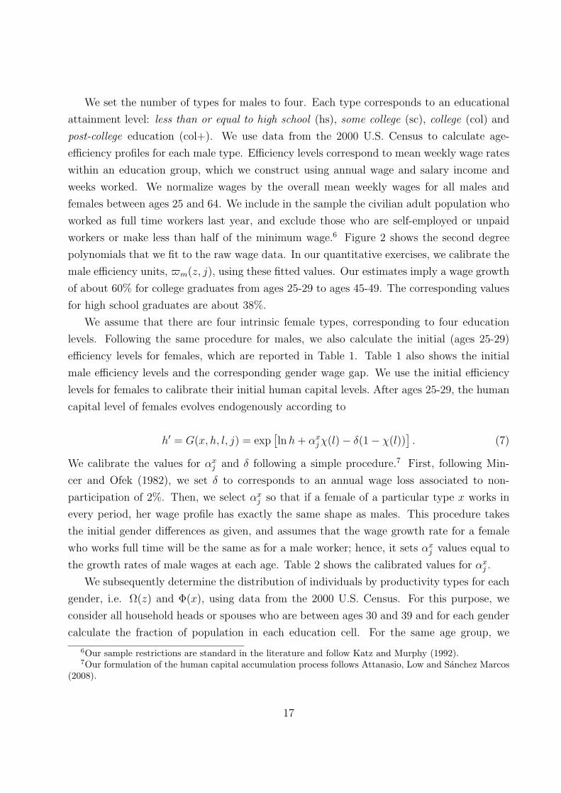
We set the number of types for males to four. Each type corresponds to an educational

attainment level: less than or equal to high school (hs), some college (sc), college (col) and

post-college education (col+). We use data from the 2000 U.S. Census to calculate age-

efficiency profiles for each male type. Efficiency levels correspond to mean weekly wage rates

within an education group, which we construct using annual wage and salary income and

weeks worked. We normalize wages by the overall mean weekly wages for all males and

females between ages 25 and 64. We include in the sample the civilian adult population who

worked as full time workers last year, and exclude those who are self-employed or unpaid

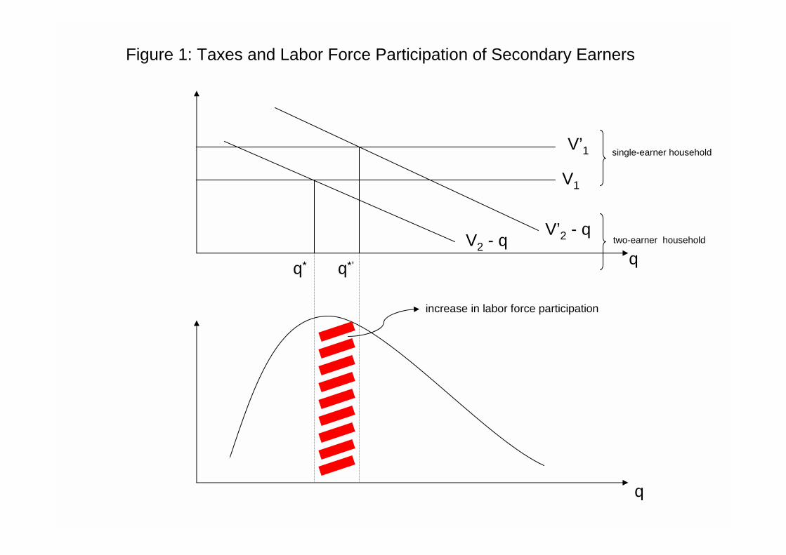
workers or make less than half of the minimum wage.6 Figure 2 shows the second degree

polynomials that we fit to the raw wage data. In our quantitative exercises, we calibrate the

male efficiency units, ϖm(z, j), using these fitted values. Our estimates imply a wage growth

of about 60% for college graduates from ages 25-29 to ages 45-49. The corresponding values

for high school graduates are about 38%.

We assume that there are four intrinsic female types, corresponding to four education

levels. Following the same procedure for males, we also calculate the initial (ages 25-29)

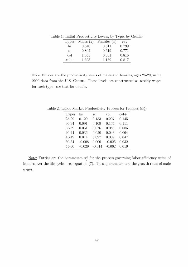
efficiency levels for females, which are reported in Table 1. Table 1 also shows the initial

male efficiency levels and the corresponding gender wage gap. We use the initial efficiency

levels for females to calibrate their initial human capital levels. After ages 25-29, the human

capital level of females evolves endogenously according to

h′ = G(x, h, l, j) = exp[lnh+ αx

jχ(l)− δ(1− χ(l))]. (7)

We calibrate the values for αxj and δ following a simple procedure.7 First, following Min-

cer and Ofek (1982), we set δ to corresponds to an annual wage loss associated to non-

participation of 2%. Then, we select αxj so that if a female of a particular type x works in

every period, her wage profile has exactly the same shape as males. This procedure takes

the initial gender differences as given, and assumes that the wage growth rate for a female

who works full time will be the same as for a male worker; hence, it sets αxj values equal to

the growth rates of male wages at each age. Table 2 shows the calibrated values for αxj .

We subsequently determine the distribution of individuals by productivity types for each

gender, i.e. Ω(z) and Φ(x), using data from the 2000 U.S. Census. For this purpose, we

consider all household heads or spouses who are between ages 30 and 39 and for each gender

calculate the fraction of population in each education cell. For the same age group, we

6Our sample restrictions are standard in the literature and follow Katz and Murphy (1992).7Our formulation of the human capital accumulation process follows Attanasio, Low and Sanchez Marcos

(2008).

17

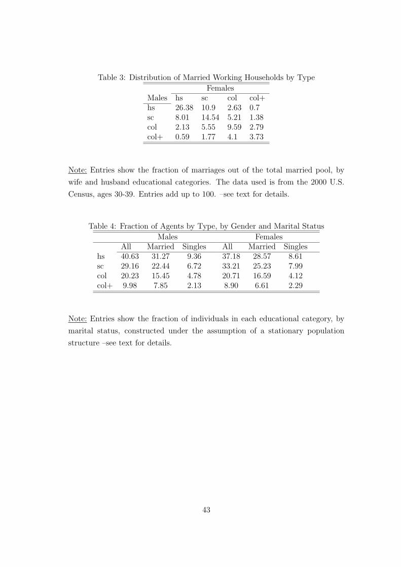
also construct M(x, z), the distribution of married working couples, as shown in Table 3.

Consistent with positive assortative matching by education, the largest entries in each row

and column in Table 3 are located along the diagonal.8

Given the fractions of individuals in each education group, Φ(x) and Ω(z), and the

fractions of married households, M(x, z), in the data, we calculate the implied fractions

of single households, ω(z) and ϕ(x), from accounting identities (1) and (2). The resulting

values are reported in Table 4: about 77% of households in the benchmark economy consists

of married households, while the rest (about 23%) are single.

Since we assume that the distribution of individuals by marital status is independent of

age, we use the 30-39 age group for our calibration purposes. This age group captures the

marital status of recent cohorts during their prime-working years, while being at the same

time representative of older age groups.

Childbearing Our model assumes that each single female and each married couple

belong to one of three groups: childless, early child bearer and late child bearer. The early

child bearers have two children at ages 1, 2 and 3, corresponding to ages 25-29, 30-34 and

35-39, while late child bearers have their two children at ages 2, 3, and 4, corresponding

to ages 30-34, 35-39, 40-44. This particular structure captures two key features of the data

from the 2002 CPS June supplement.9 First, conditional on having a child, married couples

tend to have two children.10 Second, these two births occur within a short period of time,

mainly between ages 25 and 29 for households with low education and between ages 30 and

34 for households with high education.11

For singles, we use data from the 2002 CPS June supplement and calculate the fraction

of 40 to 44 years old single (never married or divorced) females with zero live births. We use

these statistics as a measure of lifetime childlessness. Then we calculate the fraction of all

single women above age 25 with a total number of two live births who were below age 30 at

their last birth. This fraction gives us those who are early child bearers, and the remaining

8See Fernandez, Guner and Knowles (2005) for a study of positive assortative matching by education.9The CPS June Supplement provides data on the total number of live births and the age at last birth for

females, which are not available in the U.S. Census.10For married households in which women are above age 25, the total number of live births varies from

2.4 for those households in which both husband and wife have at most high school degrees to 2 for thosehouseholds in which both husband and wife have more than a college degree. For the majority of households,the total number of children is close to 2.

11The average age at first birth is 26.2 for those households in which both husband and wife have at mosthigh school degrees, and 31.1 for those households in which both husband and wife have more than a collegedegree. For the same household types with two children, the average age at second were 26.8 and 31.3,respectively.

18

fraction of assigned as late child bearers. The resulting distribution is shown in Tables 5.

We follow a similar procedure for married couples, combining data from the CPS June

Supplement and the U.S. Census. For childlessness, we use the large sample from the U.S.

Census.12 The Census does not provide data on total number of live births but the total

number of children in the household is available. Therefore, as a measure of childlessness

we use the fraction of married couples between ages 35-39 who have no children at home.13

Then, using the CPS June supplement we look at all couples above age 25 in which the

female had a total of two live births and was below age 30 at her last birth. This gives us the

fraction of couples who are early child bearers, with the remaining married couples labeled

as the late ones. Table 6 shows the resulting distributions.

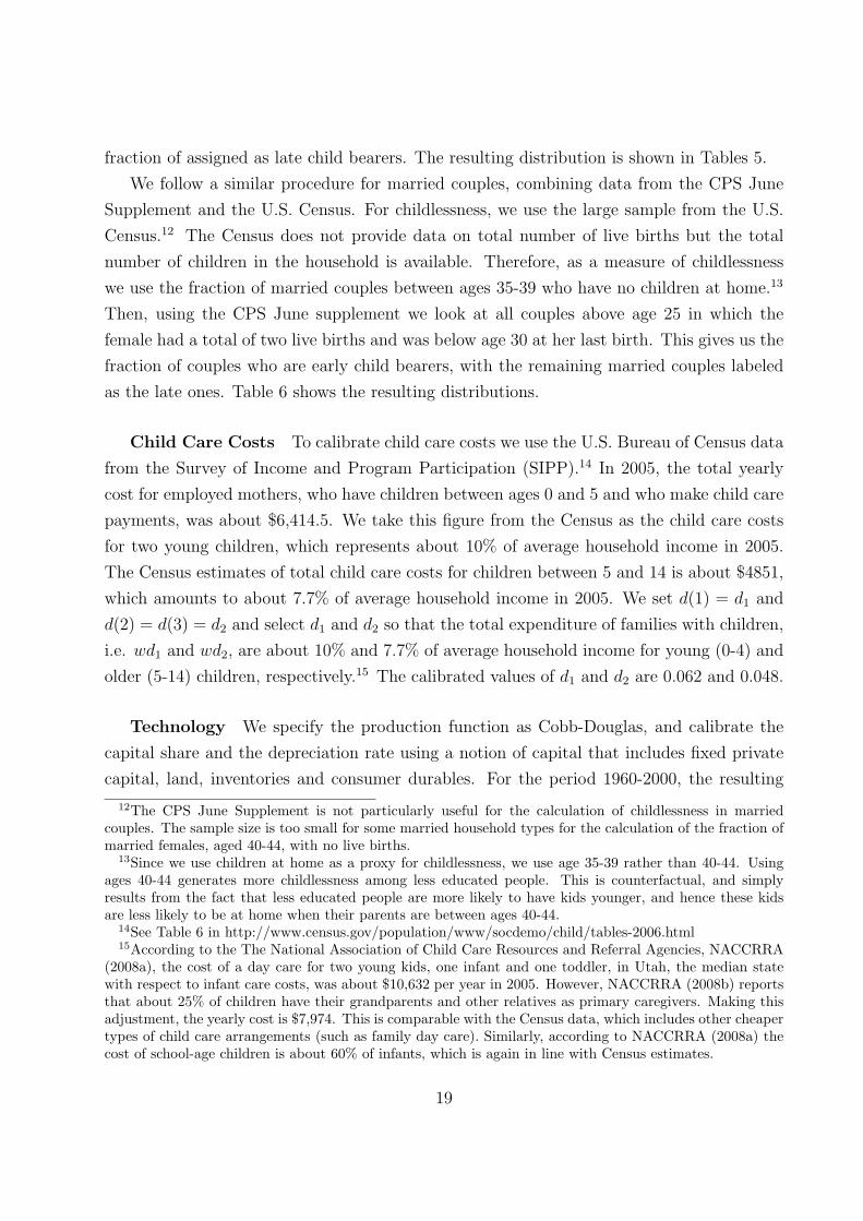
Child Care Costs To calibrate child care costs we use the U.S. Bureau of Census data

from the Survey of Income and Program Participation (SIPP).14 In 2005, the total yearly

cost for employed mothers, who have children between ages 0 and 5 and who make child care

payments, was about $6,414.5. We take this figure from the Census as the child care costs

for two young children, which represents about 10% of average household income in 2005.

The Census estimates of total child care costs for children between 5 and 14 is about $4851,

which amounts to about 7.7% of average household income in 2005. We set d(1) = d1 and

d(2) = d(3) = d2 and select d1 and d2 so that the total expenditure of families with children,

i.e. wd1 and wd2, are about 10% and 7.7% of average household income for young (0-4) and

older (5-14) children, respectively.15 The calibrated values of d1 and d2 are 0.062 and 0.048.

Technology We specify the production function as Cobb-Douglas, and calibrate the

capital share and the depreciation rate using a notion of capital that includes fixed private

capital, land, inventories and consumer durables. For the period 1960-2000, the resulting

12The CPS June Supplement is not particularly useful for the calculation of childlessness in marriedcouples. The sample size is too small for some married household types for the calculation of the fraction ofmarried females, aged 40-44, with no live births.

13Since we use children at home as a proxy for childlessness, we use age 35-39 rather than 40-44. Usingages 40-44 generates more childlessness among less educated people. This is counterfactual, and simplyresults from the fact that less educated people are more likely to have kids younger, and hence these kidsare less likely to be at home when their parents are between ages 40-44.

14See Table 6 in http://www.census.gov/population/www/socdemo/child/tables-2006.html15According to the The National Association of Child Care Resources and Referral Agencies, NACCRRA

(2008a), the cost of a day care for two young kids, one infant and one toddler, in Utah, the median statewith respect to infant care costs, was about $10,632 per year in 2005. However, NACCRRA (2008b) reportsthat about 25% of children have their grandparents and other relatives as primary caregivers. Making thisadjustment, the yearly cost is $7,974. This is comparable with the Census data, which includes other cheapertypes of child care arrangements (such as family day care). Similarly, according to NACCRRA (2008a) thecost of school-age children is about 60% of infants, which is again in line with Census estimates.

19

capital to output ratio averages 2.93 at the annual level. The capital share equals 0.343 and

the (annual) depreciation rate amounts to 0.055.16

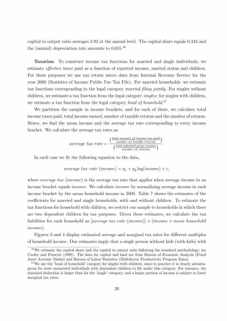
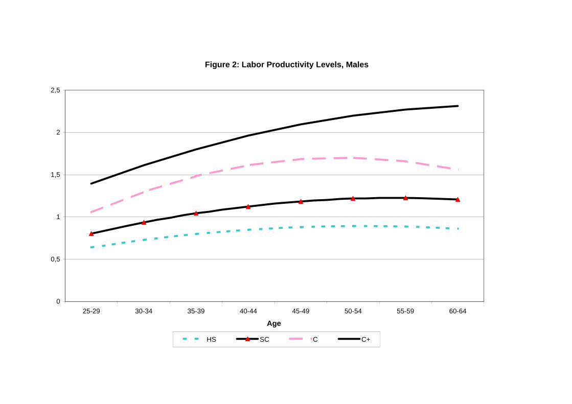
Taxation To construct income tax functions for married and single individuals, we

estimate effective taxes paid as a function of reported income, marital status and children.

For these purposes we use tax return micro data from Internal Revenue Service for the

year 2000 (Statistics of Income Public Use Tax File). For married households, we estimate

tax functions corresponding to the legal category married filing jointly. For singles without

children, we estimate a tax function from the legal category singles ; for singles with children,

we estimate a tax function from the legal category head of household.17

We partition the sample in income brackets, and for each of these, we calculate total

income taxes paid, total income earned, number of taxable returns and the number of returns.

Hence, we find the mean income and the average tax rate corresponding to every income

bracket. We calculate the average tax rates as

average tax rate = total amount of income tax paid

number of taxable returns

total adjusted gross incomenumber of returns

.

In each case we fit the following equation to the data,

average tax rate (income) = η1 + η2 log(income) + ε,

where average tax (income) is the average tax rate that applies when average income in an

income bracket equals income. We calculate income by normalizing average income in each

income bracket by the mean household income in 2000. Table 7 shows the estimates of the

coefficients for married and single households, with and without children. To estimate the

tax functions for household with children, we restrict our sample to households in which there

are two dependent children for tax purposes. Given these estimates, we calculate the tax

liabilities for each household as [average tax rate (income)] × (income ×mean household

income).

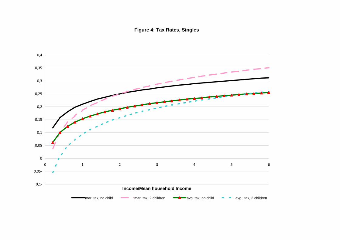
Figures 3 and 4 display estimated average and marginal tax rates for different multiples

of household income. Our estimates imply that a single person without kids (with kids) with

16We estimate the capital share and the capital to output ratio following the standard methodology; seeCooley and Prescott (1995). The data for capital and land are from Bureau of Economic Analysis (FixedAsset Account Tables) and Bureau of Labor Statistics (Multifactor Productivity Program Data).

17We use the ’head of household’ category for singles with children, since in practice it is clearly advanta-geous for most unmarried individuals with dependent children to file under this category. For instance, thestandard deduction is larger than for the ’single’ category, and a larger portion of income is subject to lowermarginal tax rates.

20

twice mean household income in 2000 faces an average tax rate of about 19.3 (15.8%) and

a marginal tax rate equal to about 24.9% (24.9%). The corresponding rates for a married

household with the same income are about 16.4% (14.6%) and 23.7% (23.6%).

Finally, we need to assign a value for the (flat) capital income tax rate τ k, which we use

to proxy the corporate income tax. We estimate this tax rate as the one that reproduces

the observed level of tax collections out of corporate income taxes after the major reforms of

1986. For the period 1987-2000, such tax collections averaged about 1.92% of GDP. Using

the technology parameters we calibrate in conjunction with our notion of output (business

GDP), we obtain τ k = 0.097. Overall, our choices imply tax collections that amount to

about 12.7% of output. The corresponding value in the data for the year 2000 was 12.3%.

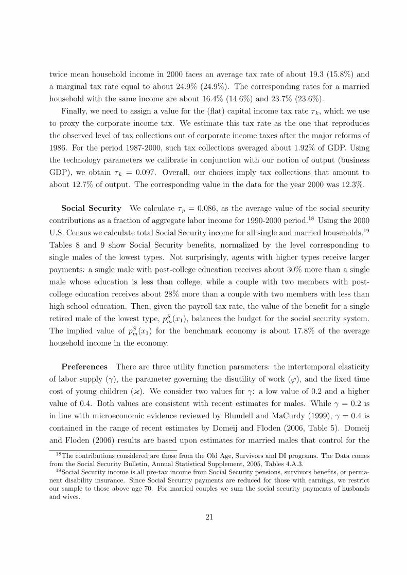
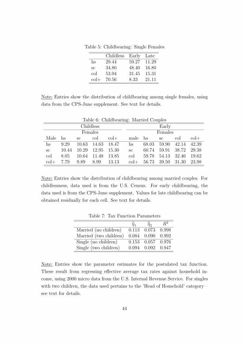
Social Security We calculate τ p = 0.086, as the average value of the social security

contributions as a fraction of aggregate labor income for 1990-2000 period.18 Using the 2000

U.S. Census we calculate total Social Security income for all single and married households.19

Tables 8 and 9 show Social Security benefits, normalized by the level corresponding to

single males of the lowest types. Not surprisingly, agents with higher types receive larger

payments: a single male with post-college education receives about 30% more than a single

male whose education is less than college, while a couple with two members with post-

college education receives about 28% more than a couple with two members with less than

high school education. Then, given the payroll tax rate, the value of the benefit for a single

retired male of the lowest type, pSm(x1), balances the budget for the social security system.

The implied value of pSm(x1) for the benchmark economy is about 17.8% of the average

household income in the economy.

Preferences There are three utility function parameters: the intertemporal elasticity

of labor supply (γ), the parameter governing the disutility of work (φ), and the fixed time

cost of young children (κ). We consider two values for γ: a low value of 0.2 and a higher

value of 0.4. Both values are consistent with recent estimates for males. While γ = 0.2 is

in line with microeconomic evidence reviewed by Blundell and MaCurdy (1999), γ = 0.4 is

contained in the range of recent estimates by Domeij and Floden (2006, Table 5). Domeij

and Floden (2006) results are based upon estimates for married males that control for the

18The contributions considered are those from the Old Age, Survivors and DI programs. The Data comesfrom the Social Security Bulletin, Annual Statistical Supplement, 2005, Tables 4.A.3.

19Social Security income is all pre-tax income from Social Security pensions, survivors benefits, or perma-nent disability insurance. Since Social Security payments are reduced for those with earnings, we restrictour sample to those above age 70. For married couples we sum the social security payments of husbandsand wives.

21

bias emerging from borrowing constraints.20 We proceed by presenting first results when

the intertemporal elasticity of substitution equals 0.4. In subsequent sections, we discuss

the implications of a lower value for this parameter. Given γ, we select the parameter φ to

reproduce average market hours per worker observed in the data. These average hours per

worker amounted to about 40.1% of available time in 2000.21 We set κ = 0.141 to match

the labor force participation of married females with young, 0 to 4 years old, children. From

the 2000 U.S. Census, we calculate the labor force participation of females between ages

25 to 39 who have two children and whose oldest child is less than 5 as 55.6%. We select

the fixed cost such that the labor force participation of married females with children less

than 5 years (i.e. early child bearers between ages 25 and 29 and late child bearers between

ages 30 and 34), has the same value.22 Finally, we choose the discount factor β, so that the

steady-state capital to output ratio matches the value in the data consistent with our choice

of the technology parameters (2.93 in annual terms).

This leaves us with the utility cost of joint work, q, to determine. Note that even without

this utility cost, married females face a non-trivial labor force participation decision due to

child care costs and human capital accumulation. The presence of utility costs associated to

joint work allows to capture residual heterogeneity among couples, beyond heterogeneity in

endowments and children, that is needed to generate observed labor supply behavior, and in

particular, labor force participation. As we explain in Section 2, all else the same, couples for

which utility costs are high will have one earner whereas those with low costs will have both

members in the labor force. Public policy via taxes and transfers will affect this decision

and thus, the resulting degrees of labor force participation.

We assume that the utility cost parameter is distributed according to a (flexible) gamma

distribution, with parameters kz and θz. Thus, conditional on the husband’s type z,

q ∼ ζ(q|z) ≡ qkz−1 exp(−q/θz)Γ(kz)θ

kzz

,

where Γ(.) is the Gamma function, which we approximate on a discrete grid. By proceeding

20Rupert, Rogerson and Wright (2000) provide estimates within a similar range in the presence of a homeproduction margin. Heathcote, Storesletten and Violante (2009) report an estimate of 0.38, using a modelwith incomplete markets.

21The numbers are for people between ages 25 and 54 and are based on data from the Consumer PopulationSurvey. We find mean yearly hours worked by all males and females by multiplying usual hours worked ina week and number of weeks worked. We assume that each person has an available time of 5000 hours peryear. Our target for hours corresponds to 2005 hours in the year 2000.

22Our calibrated value for κ is in the ballpark of available estimates in the literature. Hotz and Miller(1988) estimate that the time cost of a newborn is about 660 hours per year and this cost declines at 12%per year. This would imply that parents spend about 520 hours per children, who are between ages 0 and5. With 5000 available hours per year, this is more than 10% per child.

22

in this way, we exploit the information contained in the differences in the labor force partic-

ipation of married females as their own wage rate differ with education (for a given husband

type). We emphasize that this allows us to control the slope of the distribution of utility

costs, which is potentially important in assessing the effects of tax changes on labor force

participation.

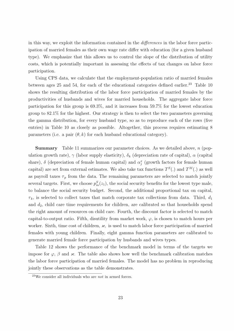
Using CPS data, we calculate that the employment-population ratio of married females

between ages 25 and 54, for each of the educational categories defined earlier.23 Table 10

shows the resulting distribution of the labor force participation of married females by the

productivities of husbands and wives for married households. The aggregate labor force

participation for this group is 69.3%, and it increases from 59.7% for the lowest education

group to 82.1% for the highest. Our strategy is then to select the two parameters governing

the gamma distribution, for every husband type, so as to reproduce each of the rows (five

entries) in Table 10 as closely as possible. Altogether, this process requires estimating 8

parameters (i.e. a pair (θ, k) for each husband educational category).

Summary Table 11 summarizes our parameter choices. As we detailed above, n (pop-

ulation growth rate), γ (labor supply elasticity), δk (depreciation rate of capital), α (capital

share), δ (depreciation of female human capital) and αxj (growth factors for female human

capital) are set from external estimates. We also take tax functions T S(.) and TM(.) as well

as payroll taxes τ p from the data. The remaining parameters are selected to match jointly

several targets. First, we choose pSm(z1), the social security benefits for the lowest type male,

to balance the social security budget. Second, the additional proportional tax on capital,

τ k, is selected to collect taxes that match corporate tax collections from data. Third, d1

and d2, child care time requirements for children, are calibrated so that households spend

the right amount of resources on child care. Fourth, the discount factor is selected to match

capital-to-output ratio. Fifth, disutility from market work, φ, is chosen to match hours per

worker. Sixth, time cost of children, κ, is used to match labor force participation of married

females with young children. Finally, eight gamma function parameters are calibrated to

generate married female force participation by husbands and wives types.

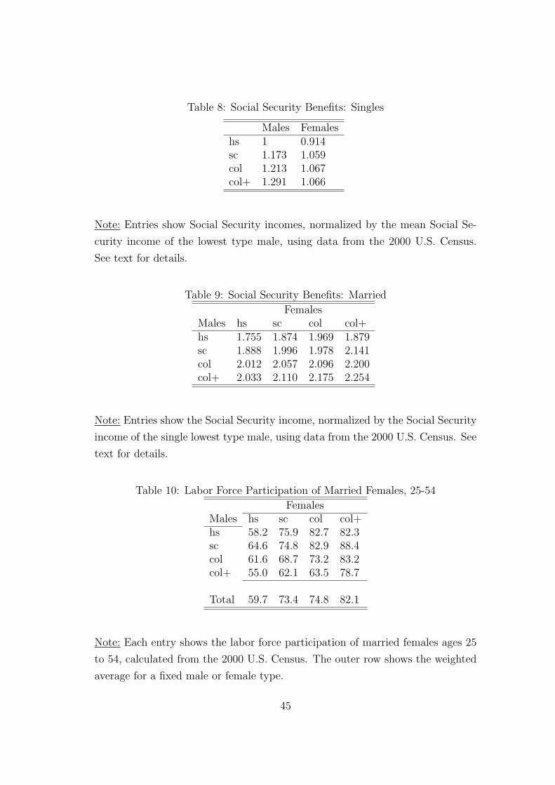
Table 12 shows the performance of the benchmark model in terms of the targets we

impose for φ, β and κ. The table also shows how well the benchmark calibration matches

the labor force participation of married females. The model has no problem in reproducing

jointly these observations as the table demonstrates.

23We consider all individuals who are not in armed forces.

23

4.1 The Benchmark Economy

Before proceeding to investigate the effects of tax reforms, we report on properties of the

benchmark economy, and compare these with the corresponding values from data. This is

critical for the questions at hand: to conduct tax reforms within our framework we want to be

confident that it offers a good model of female labor supply. We focus on different aspects of

the model economy here. In particular, (i) how does female labor force participation change

by age and the presence of children? (ii) what is the gender gap in our model economy?

The answer to the first question is important since the interaction between children and

female labor force participation plays a key role in our model. The answer to the second

question is also critical, since married females in our economy have a non-trivial labor force

participation decision which results in an endogenous gender gap. In assessing the model

performance, it is important to bear in mind that the empirical targets for the model are

the levels of aggregate participation rates by marriage type, and the participation rates of

women with young children. No age-related statistics are used, so the match between model

and data in this dimension is due to the forces governing household labor supply within the

model.

At the aggregate level, the model is in conformity with data. The model reproduces,

by construction, the labor force participation rate of women with young children and the

economy-wide level of participation, as it targets participation rates by type. It also captures

the consequences of the presence of children on participation rates. Participation rates of

women with children are lower than those without children, both in the model and in the

data; about 64.4% versus 67.4%. Females without children participate more, their labor

force participation are 82.9% and 82.5% in the model and in the data, respectively.

What are the female labor supply elasticities implied by the model economy? Although

there are different ways one can measure the elasticity of female labor supply, given our

model a natural one is to ask how much female labor force participation and aggregate

hours will increase if female productivity levels were increased by 1%. Our model implies

an aggregate elasticity of female labor force participation to changes in female productivity

levels of about 0.72 and an aggregate elasticity of total hours worked by married females

to changes in female productivity levels of about 0.95.24 If we were to calculate the same

elasticities to changes in the economy wide wage rate, we find elasticities of 0.36 and 0.35,

respectively, which are (not surprisingly) lower.25

24These elasticities are in line with estimates surveyed in Blundell and MaCurdy (1999) and Keane (2010).25Consistent with available empirical evidence, elasticity of male hours with respect to the wage rate is

about zero.

24

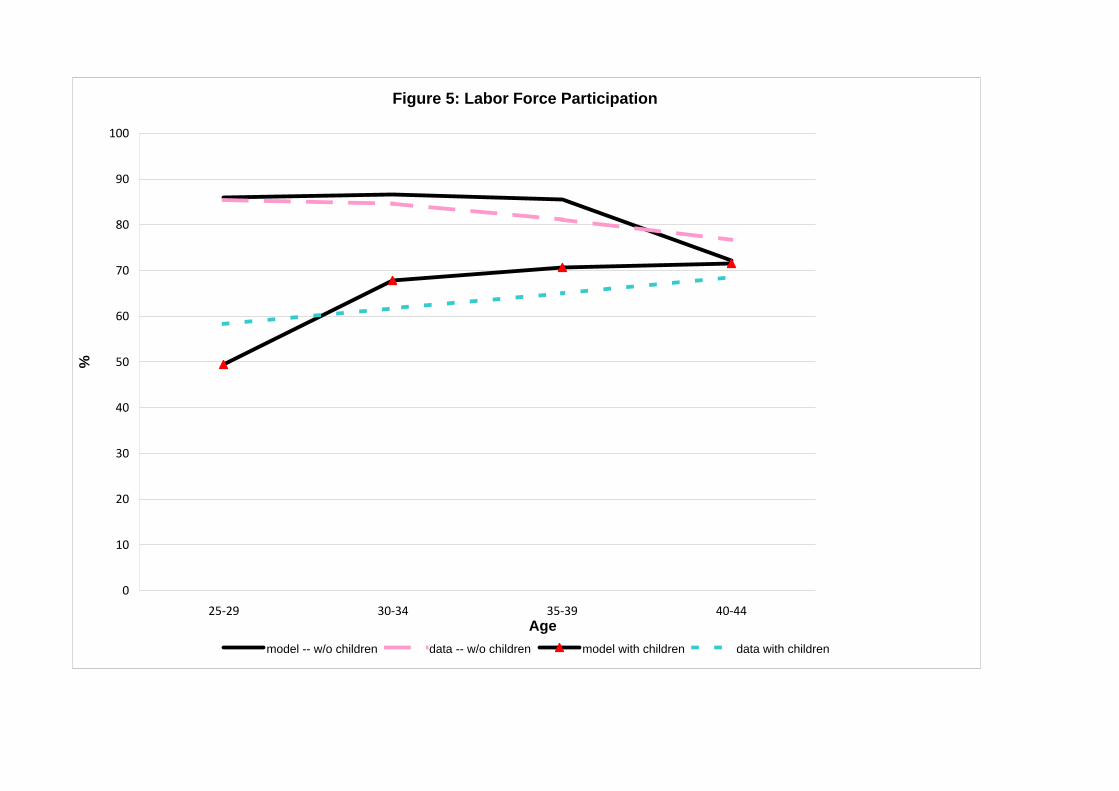
Figure 5 shows married female labor force participation by age and by the presence of

children. As the figure shows, the labor force participation of married females with children

increases monotonically with age both in the model and the data, and its level is always

below that for women without children. Both in the model economy and the data, those

who have their children early on, at ages 25-29, are women with low levels of education; not

surprisingly, their labor force participation is low. Those who have their children in later

ages tend to be skilled women, whose labor force participation is higher. Furthermore, those

who have their children early are more likely to participate in the labor market in later ages,

since their children age and the associated child care costs decline. The participation rate of

women without children, on the other hand, declines slightly between ages 25-29 to 40-44.

The decline in later ages is mainly due to women who had their children in the first period

and enter the labor force in later ages as these children age. Since these women are mainly

from lower education groups and could not accumulate human capital in the initial years,

they have low labor force participation.

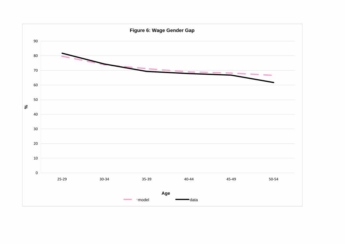
Figure 6 displays the wage gender gap in the model and the data. In the model economy

we observe the labor market productivity levels for all females, whether they participate in

the labor market or not. Since this is a more informative statistic, we report the gender

gap from the model for all females. In order to produce a comparable measure from the

data, we have to impute wages for females who do not participate in the labor market. In

order to do that, we estimate a standard Mincer regression with Heckman (1979) selection

correction, which provides us with wage estimates for women who do not participate in the

labor market. When we report data on wages, we report an average of observed wages (for

women who work) and imputed wages (for women who do not work). What is critical is that

Heckman’s procedure allows us to assign a wage for females who do not work.26 The model

does a very good job in generating both the level and the age pattern of the wage gender

gap. In interpreting these results, it is important to bear in mind that wage gender gap is

critically determined by labor force participation decisions. Moreover, we have selected the

parameters of human capital accumulation process for females a priori without targeting any

endogenous variables. Both in the data and the model, the ratio of female to male wages

starts at about 80% and declines monotonically as women age, reaching less than 65% by

26For the population equation for wages, we assume that log wages of women depend on years of education,age, age-squared and an interaction between age and years of education. For the selection equation, weassume that the probability of participation in the labor market for a female depends on her marital status,number of children younger than age 5, and the variables in the population equation. We estimate theparameters using Maximum Likelihood and use the corrected parameters of the Mincer equation to imputewages for women with missing wages. Our selection equation is similar to ones used by Chang and Kim(2006) and Mulligan and Rubinstein (2008).

25

age 54. The average gender gap for ages 25 to 54 is about 70%. As women with children

decide to stay out of the labor force, their human capital declines generating endogenously

a larger gender gap in later ages.27, 28

The Importance of Costly Childbearing What is the quantitative importance of

childcare costs in the benchmark economy? To this end, and motivated by the evidence

presented earlier in this section, we run two counterfactual exercises. First, we double the

child care expenses for working mothers, by doubling d(s) values. This has a dramatic

effect on female labor force participation. Female labor force participation declines by about

twenty percent (from 69.3% to 55.4%). As a result, aggregate hours and output decline

by 4.1% and 5.7%, respectively. Second, we double the fixed time cost for children. With

higher time costs, married female labor force participation declines by 8.4% (from 69.3% to

63.5%). The effect is much stronger for married females with young children, as their labor

force participation declines by 80%. As with the higher child care costs, aggregate hours and

aggregate output declines by about 1.9% and 4.1%, respectively. Hence, variation in child

care costs critically matters in the determination of participation decisions. We conclude

that the modeling of costs associated to children is of central importance for labor supply

decisions at the household level.

Participation Rates and the Temporal Variation in Wages What are the impli-

cations for labor force participation rates, within our model, of a wage structure consistent

with observed ones in the past? The answer to this question is important in assessing whether

our model generates female labor force participation responses that are reasonable from a

time-series point of view. To this end, we parameterize our economy with the wage structure

of 1970, i.e. we take male wages for all ages and types as well as initial (age-1) wages for

males from 1970 data. We keep all other parameters in their benchmark values. We find that

in this scenario, female labor force participation declines by 2.3 percentage points relative

to our benchmark, or about 10% of the observed change in the data.

27Our results on the gender gap are quite similar to those by Erosa, Fuster and Restuccia (2010). Theyalso show that differences in human capital accumulation explain the widening gender gap over the life-cycleand children play a key role in determining lower human capital accumulation by females.

28Note that in the simulations, the initial (age 25-29) human capital levels for females are set accordingto data in Table 1. In the data, these initial productivity levels are calculated for females who participatein the labor market. In the model, females observe these initial productivity levels and then decide whetherto work or not. Hence, the gender gap in the model is exactly same as the observed gender gap in the data(79.9%). This is almost identical to corrected gender gap in Figure 6 (81.7%) as selection does not play arole for this age group.

26

Childcare services were more expensive in 1970; see Attanasio et al (2008). Hence, if in

addition we increase the values of child cost parameters that we get from the first experiment

by 25%, aggregate labor force participation drops by about 5.2 percentage points.29 This

indicates that the model accounts for about 21% of the observed change in the data. Given

that many other factors changed from 1970 to 2000 (i.e. the structure of taxes as well as

the marital structure of population), we conclude from these findings that the underlying

elasticities in our model are sensible, as the model does not overshoot the observed decline

in participation from 2000 to 1970.30

5 Tax Reforms

We now consider two hypothetical reforms to the current U.S. tax structure: a proportional

income tax and a move from joint to separate filing for married couples. The first reform

flattens the current income tax schedule while keeping the household as unit subject to

taxation. The second reform reintroduces progressivity into the system, but changes the

unit of taxation from households to individuals. The proportional income tax allows us to

illustrate the effects of a rather well-studied case within the current framework, and relate

our results with the existing literature. The second reform, which is impossible to analyze

within a standard single-earner framework, illustrates the value-added of the model features

of the current framework.

The findings we report are based on steady-state comparisons of pre and post-reform

economies. In all cases, we keep the social security tax rate unchanged, which implies that

benefits adjust with the reforms under consideration. For our benchmark set of experiments,

we also keep the residual tax rate on capital income (τ k) fixed. The exercises are in all cases

revenue neutral.

5.1 A Proportional Income Tax

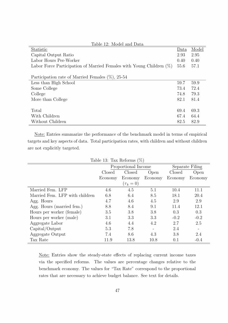
Table 13 reports the key findings from this exercise. To assess these results, the reader should

bear in mind that by construction, a proportional income tax makes marginal and average

tax rates equal for all households. Before the reform average and marginal tax rates covered

29A 25% decline in child care costs is empirically plausible. Attanasio et al (2008) document that the levelof child care costs declined by 15% between 1970s and 1980s and that the decline relative to female wageswas even larger. Since the 1970s, the tax treatments of child care expenses has also become more favorable.Arguably, the availability of child care has improved significantly as well.

30See Kaygusuz (2010) for a decomposition of the changes in the post-1980 increase in female labor supplyinto parts that come from changes in taxation, wages, educational attainment and marital structure, in anenvironment without children.

27

a wide range, as indicated in Figures 3 and 4; in the new steady state, the uniform tax rate

that balances the budget equals 11.9%. Thus, via the removal of distortions associated with

a progressive income tax, this reform leads to substantial effects on output and factor inputs.

The capital-to-output ratio increases by about 5.3% across steady states, leading to changes

in the wage rate of about 2.4%. Total labor supply (hours adjusted by efficiency units)

increases by 4.6%. As a result of these changes, aggregate output increases substantially by

about 7.4%.

Our economy allows us to identify and quantify differential responses in labor supply

to tax changes that take place at the intensive margin for both males and females, as well

as at the extensive margin for married females. Recall that in the benchmark economy,

the tax structure generates non-trivial disincentives to work since average and marginal tax

rates increase with incomes. In addition, married females who decide to enter the labor

force are taxed at their partner’s current marginal tax rate. With the elimination of these

disincentives, the change in labor supply of married females is substantially larger than the

aggregate change in hours. The introduction of a flat-rate income tax implies that the labor

force participation of married females increases by about 4.6%, while hours per worker rise

by about 3.5% for females, and about 3.1% for males. Due to changes along the intensive

and the extensive margins, total hours for married females increase by about 8.8%. This is

a dramatic rise and is nearly three times the changes in total male hours. These results are

especially worth noting as the parameter governing intertemporal substitution of labor is the

same for males and females, and take place despite the equilibrium increase in the cost of

child care (i.e. the wage rate goes up).

It is important to highlight three aspects of the results emerging from this experiment.

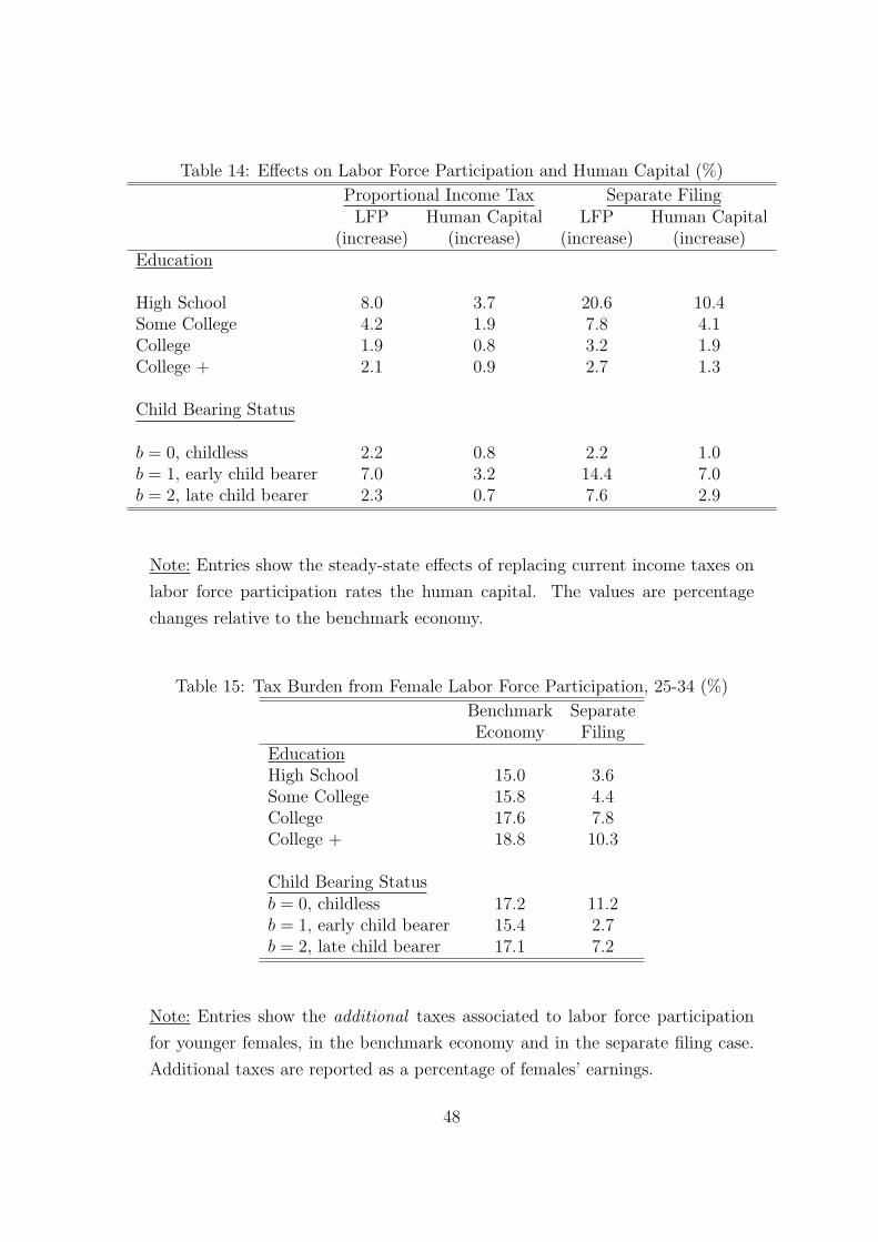
First, as we show in Table 14, low-type married females increase their labor supply much

more than high-type females. Over the life cycle, females with the lowest intrinsic type (those

with high school education or less) increase their labor force participation by 8.0%, while

highest types (those with post-college education) increase theirs only by 2.1%. This might

come as a surprise, since a proportional income tax reform would likely increase marginal tax

rates for lower types and reduce them for high types. There are several reasons that account

for this phenomenon. Note first that the labor force participation of high-type married

females is quite large in the benchmark economy to begin with, leaving relatively little room

to react to tax changes. Secondly, relative to the benchmark economy, marginal tax rates

effectively drop or remain relatively constant for low and middle income households after

the introduction of the proportional income tax. In the benchmark economy, the marginal

tax rate on a household with an income equal to one half average income is about 11%,

28

little less than the rate after the reform, while the marginal rate amounts to about 17.4%

for those with a mean income level. In other words, a proportional tax leads to a reduction

in marginal tax rates even for low and middle-income households in the new steady state.31

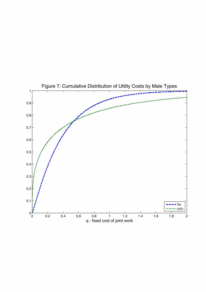
Finally, the relative shapes of the distributions (cdf) of utility costs clearly indicates the

scope for a much larger reaction of less skilled types. We plot in Figure 7 the distributions

for a married household with a husband with more than college education, as well as the

distribution for a household with a husband with high school education. As it can be seen,

the slopes of the distributions are much larger for a typical less-skilled couple (both with high

school or less) versus a typical high skilled couple (both with more than college education).

Hence, it is easy to see that tax changes leading to changes in participation will have larger

effects for less skilled females.

Second, the response of married females with children is larger than those without chil-

dren, as Table 13 and the lower panel of Table 14 demonstrate. While for married females

who are childless the labor force participation increases by about 2.2%, the rise is much

larger, about 7.0%, for those who are early child bearers, whereas the response increases

up to about 10.5% for those with young children. This phenomenon is connected with the

reasons for females with children to react more strongly to tax changes (see section 2), and

to the stronger participation reaction of less-skilled females discussed above; lower types are

more likely to have children as well as to have them early.

Finally, the increasing labor force participation of married females leads to higher effi-

ciency units (human capital) for this group, by about 1.9%. As we document in Table 14,

the increase in human capital is larger for lower types and those with children, which reflects

the changes in labor force participation. It is about 3.7% for those with less than high school

education, in contrast to nearly 1% for those with post-college education.

Eliminating τ k In Table 13, we also report the results where we eliminate τ k in a propor-

tional income tax reform. Note that the tax rate that balances the budget is obviously higher

when the capital income tax rate is included (13.8% versus 11.9%), as larger tax collections

need to be generated. The results indicate that the inclusion of the flat-rate capital income

tax in the tax reforms is largely unimportant for the magnitudes of labor supply responses.

The key differences where τ k is kept intact are in the magnitude of output changes: when

the capital income tax is included in the reform, output changes amount to 8.6% versus 7.4%

31We abstract from means-tested welfare programs, such as food stamps and Medicaid. It is well knownthat such programs can generate very high marginal tax rates at low levels of income, as earning more mightimply not qualifying for benefits; see Moffitt (1992) and Meghir and Phillips (2010). These programs arelikely to dampen the responses by lower income households.

29

when the capital income tax rate is maintained.

These differences are due to the larger effects on capital accumulation that take place

when the capital income tax rate is eliminated in the tax reform. This is simply accounted

for by the different tax burden on capital in the two cases. When the capital income tax

rate is part of the reform, the effective tax rate on capital income is simply 13.8% (i.e. the

income tax rate), whereas it is much higher (21.6%, which is the sum of the proportional

tax, 11.9% and τ k, 9.75%) when the reform does not include the flat-rate capital income tax.

5.2 Separate Filing

A prominent feature of the current U.S. tax system is that it treats married and single

individuals differently. The problem arises since the unit subject to taxation is the household,

not the individual, with tax schedules that differ according to marital status. This creates

much discussed marriage-tax penalties and bonuses, affecting the marginal tax rates that

married individuals face. In particular, note that when a married female enters the labor

market the first dollar of her earned income is taxed at her husband’s current marginal rate,

potentially distorting her labor supply in a critical way. This reasoning motivates our second

experiment, where we move from the current system to one in which each individual files

his/her taxes separately. We label this hypothetical reform experiment separate filing.

We assume that a married person’s tax liabilities consists of his/her labor income plus

half of household’s asset income, and each working member of a married household with

children declares one of the two children for tax purposes. In particular, for a married

household without children we use the same tax function that singles without children face

in the benchmark economy. For married households with children, we use a tax function

from the legal category head of household (with one child) for each member. In addition, in

order to collect the same amount of tax revenue as the benchmark economy, we assume that

each individual faces an additional proportional tax (or subsidy) on his/her income.32

The possibility of separate filing can lower taxes on married females significantly.33 To

see this, consider a married household with kids with total income equal to twice mean

household income, and suppose earnings of both members are equal. Under the current

system, this household faces a marginal tax rate of about 23.6%. The marginal tax rate

declines to about 17.4% if the household income is split equally between husband and wife.

32We estimate a tax function for heads of households with one child, resulting in parameters η1 = 0.107 andη2 = 0.082. In stationary equilibrium after the reform, a tax of 0.1% is needed to achieve revenue-neutrality.

33In contrast to Alessina, Ichino and Karabarbounis (2009), lower taxes on females emerge in the currentframework from taxing individuals instead of households, and not from an optimal taxation argument tolower taxes on females who have more elastic labor supplies.

30

The gain is larger for the majority of wives who earn less than their husbands.

The effects of a move from the current system to separate filing are substantial. Table 13

shows that aggregate output goes up by about 3.8%, and aggregate labor by 2.7%. This is

more than half of the increase associated with a proportional income tax reform. In contrast

to a proportional income tax reform, however, the increase in aggregate labor is almost fully

driven by the rise in aggregate hours by married females. The labor force participation of

married females rises by 10.4% (more than twice as much as it does with a proportional

income tax), and aggregate hours by married females increase by about 11.4%. In contrast,

hours by male workers decline slightly. As it is shown in Table 14, separate filing generates

significant increases in labor force participation and declines in gender gap for exactly the

same groups that were affected by proportional taxes, married females with less education

and with children, but with much larger magnitudes.

Why does married female labor force participation react so much with separate filing?

The key is that separate filing reduces the tax burden associated with female labor force

participation dramatically. Table 15 shows the extra taxes that a household has to pay as

a fraction of the extra income that a female generates for younger households (aged 25-34).

In the benchmark economy, the tax burden associated with female labor force participation

is quite similar for females with different characteristics. It is larger for females with more

education and for those who do not have any children. With separate filing, the situation

is radically different.34 Now females with lower education as well as those with children

face much lower tax rates associated with movements along the extensive margin. Not

surprisingly, their labor force participation increases dramatically. Incidentally, these are

the groups that have the largest potential response to a tax reform.

The main message from this policy experiment is quite clear. A move from the current

system to one in which individuals (not households) are the basic unit of taxation goes a

long way in generating significant effects on aggregate labor and output. These effects take

place without eliminating tax progressivity, or the taxation of capital income, and depend

critically on the response of married females. These and previous findings motivate us to

explicitly quantify the relative importance of married females as a group for our results. We

do this in section 6.

34In the proportional tax reform case, the extra taxes associated to further labor market participationnaturally amount to the equilibrium tax rate (11.9%).

31

5.3 Tax Reforms in an Open Economy

A concern with analysis of tax reforms in equilibrium models is the (typically) large effects on

capital intensity and output driven by the reduction or elimination of distortions on capital

accumulation. To address this issue, we conduct tax reform exercises under the assumption

of a small economy open to capital movements. We fix the before-tax rate of return on

capital at the benchmark level, and thus the wage rate, and calculate stationary equilibria

under the proposed tax systems.

Our main findings are summarized in Table 13, alongside the results from our main

experiments. As the Table shows, the effects on output are more moderate, as by construction

the ratio of capital to labor in the production of goods is the same across steady states.

However, a different picture emerges for the effects on labor supply. For instance, if a

proportional income tax is considered, labor force participation (aggregate hours) increases

by about 5.1% (4.5%) in the small-open economy case, whereas the corresponding increase

is very similar, about 4.6% (4.7%) under the closed economy assumption. A similar pattern

holds under a separate filing reform, and for different labor supply statistics. We conclude

from these exercises that the effects of tax reforms on labor supply at multiple levels are

essentially independent on whether the economy is open to capital movements or not.

5.4 Tax Reforms and Within-group Inequality

Our economy is parameterized considering only heterogeneity associated to schooling levels.

As a result, the benchmark economy produces less dispersion in wages and earnings than the

data. We calculate, using estimates from Heathcote, Storesletten and Violante (2004) for

males, that the variance of log-wages in our first (fourth) age group is about 0.177 (0.240),

while it is only 0.066 (0.089) in the model for males. This implies that our model accounts

for about 37.3% (37.1%) of the variance of log-wages for males at the start (middle) of the

life cycle.35 More generally, our model implies an economy-wide Gini coefficient of household

earnings of about 0.283. Heathcote, Perri and Violante (2010) report a corresponding value

of about 0.4 for the year 2000.

Since the model accounts for only a fraction of observed wage inequality, we assess the

robustness of our results to the explicit consideration of wage heterogeneity within education

levels. We introduce wage heterogeneity within educational groups for both males and

females in a simple way at the start of the life cycle. In particular, we assume that for each

35We use for these purposes the authors’ estimates for the structure of fixed effects and permanent shocksto wages. We exclude temporary shocks.

32

education category, there are two types, high and low, and half of each education group is

high type and the other half is low type. For males, high (low) types have ∆% higher (lower)

wages than the average wage for a given education group at any point along the life-cycle.

For women, high (low) types imply ∆% higher (lower) wages at age 1 and female wages

evolve endogenously afterwards as in the benchmark economy. Our strategy is to select ∆

to generate, inside the model, the wage dispersion for males at age 1 (variance of log-wages)

observed in the data according to Heathcote et al (2004) estimates. Our specification implies

that required ∆ is about 39.5%; i.e. high (low) types males and females at age-1 observe

wages that are 39.5% above (below) the education-specific means. Given these estimates,

we parameterize again our model economy in line with the discussion in Section 4.36

We find that the aggregate effects of reforms become more moderate with the inclusion

of within-group inequality. Under a proportional tax (separate filing), output increases by

about 6.8% (3.4%), and aggregate hours by 4.2% (2.7%). Under the benchmark specification,

increases in output were 7.4% (3.8%) under a proportional tax (separate filing) reform, while

aggregate hours increased by 4.7% (2.9%). At the center of the moderation in responses is

the behavior of labor force participation rates. Under a proportional tax (separate filing),

the participation rate of married females increases by about 2.8% (9.5%); the corresponding

changes under our benchmark specification are 4.6% (10.4%).

The smaller changes in participation rates in the case of the proportional income tax

reform are in turn driven by the behavior of married women in poorer households. With

within-group heterogeneity, taxes actually go up for a large group of women with low levels

of wages. As a result, the labor supply of response of these women with is now more muted.

This happens in much smaller magnitudes, however, when we consider the separate filing

case (i.e. a progressive tax scheme); labor force participation responses become very similar

to the ones under the benchmark scenario in the absence of within-group inequality. We

conclude from these exercises that the simple consideration of within-group inequality leads

to moderately smaller effects on aggregates upon a reform, especially in the separate filing

case. Our benchmark specification appears to capture the bulk of output and labor supply

responses upon tax reforms.

36We assume that child bearing status, marital status, wage growth factors for females, social securitybenefits depend only on agents’ education level as in the benchmark economy. Within a particular educationpair, couples are assumed to match randomly according to their high/low types.

33

6 The Role of Married Females

We now discuss in more detail the impact of changes in labor supply of married females. We

ask: what is the overall contribution of married females to changes in labor supply? What

is the importance of labor supply changes along the extensive margin?

In answering these questions, we first note that the type of the tax reform under consid-

eration is critical. As expected from the results in the previous section, the role of married

females is largest with a move to separate filing. Table 16 makes these points clear. In

this table we report the contribution of married females to changes in total hours and total

labor supply under our benchmark calibration. For proportional income taxes, the contri-

bution of married females to changes in total hours (labor supply) is around 51% (48%).

Under separate filing they contribute to more than 100% of the changes in total hours and

labor supply, as some groups effectively reduce their hours (e.g. men). We conclude from

these findings that the overall contribution of married females to hours and labor supply

changes is substantial; they contribute disproportionately given their share of the working

age population (about 37.5%).

In the bottom panel of Table 16 we focus on the role of the extensive margin and report its

contribution to the rise in hours and total labor supply. In order to assess the role of extensive

margin, we carry out the following counterfactual exercise. For each age and (x, z, q, b)-

type married woman we determine the labor force participation status in the benchmark

economy.37 Next, we run the tax reforms in an economy where the labor force participation

decision is no longer a choice for a female. The female workers in the benchmark economy

can change their hours in response to a tax reform, however, they are not allowed to drop

out of the labor force. Moreover, the females who are out of the labor force in the benchmark

economy are not allowed to enter the labor market. This allows us to quantify the significance

of the intensive margin as well as the extensive margin in the tax reform exercises. We find

that the extensive margin contributes about 25% of the changes in total hours under a

proportional income tax, and about 86% of the changes in hours under separate filing. For

changes in labor supply, the contributions are about 23% and 79%, respectively. By this

measure, these calculations suggest that the bulk of the rise in the labor supply of married

females can be attributed to movements along the extensive margin.

Married Females with Children How much of the increase in extensive margin

and aggregates hours can be attributed to married females with children? As our results

37Note that age, x, z, q, and b are exogenous characteristics of a married household.

34

in Tables 13 and 14 show their labor supply increase more than married females without

children. In order to highlight the role of females with children, we report in Table 16 the

contribution of married females with children to overall changes in hours and labor supply.

As the table demonstrates, the contribution of this group is substantial. Under a proportional

tax, married females with children account for about 21% and 18% of the changes in hours

and labor supply. In line with our previous discussion, these figures are bigger under a

separate-filing reform: 57% and 49%, respectively.

To isolate further the contribution of married females with children we focus on the

separate filing case, and consider the following version of it. Suppose only married females

without children are allowed to file separately, while married females with children file taxes

as they did in our benchmark economy. Not surprisingly, labor supply responses are much

more muted with this reform. The labor force participation of married females increases by

3.3% (in contrast to 10.4% in separate filing reform) and aggregate labor supply increases by

1.1% (in contrast to 2.7%), respectively. Hence, when we do not allow married females with

children to file separately the effect on married female labor force participation is about 70%

smaller, while the effects on aggregate labor are smaller by 60%. Hence, not only married

females account for a large part of the changes in labor supply, a large part of this change

comes from married females with children.

7 The Importance of the Intertemporal Elasticity

We now turn our attention to the role of the preference parameter γ; the micro intertemporal

elasticity of labor supply. For these purposes, we report results for the value on the low side of

the empirical estimates for this parameter (γ = 0.2), and calibrate the rest of the parameters

following the procedure discussed in Section 4. The main results are summarized in Table 17.

Our central findings are that while changes in hours per-worker are lower than under γ = 0.4,

the relative importance of changes along the extensive margin is larger under γ = 0.2. As

a result, the response of aggregate hours (and output) across steady states is not critically

affected by a lower intertemporal elasticity.

Consider first the proportional income tax reform. As we have documented in Table 16,

with γ = 0.4 about 18% of the increase in aggregate labor supply was due to higher labor

force participation by married females (i.e. due to extensive margin), while the rest came

from higher per-worker hours. With a lower γ, changing labor supply along the intensive

margin is more costly and therefore, changes along this margin are now about 40-45% lower

than they were with a higher γ. However, aggregate hours (output) still increase by as much

35

as 3.7% (6.1%), or about 78% (82%) of its increase with a high γ. This occurs since the

increase along the extensive margin is now higher; the labor force participation of married

females increases by 6.4% in contrast to a 4.6% increase under the high γ value. The net

result is that the increase in aggregate hours by married females is not much affected by a

lower γ. With an extensive margin playing a larger role now, the contribution of married

females to changes in labor hours and labor supply goes up. As Table 17 shows, while the

contribution of married females to changes in hours was 51.1% under γ = 0.4 , it is now

67%.

Since the extensive margin plays a much bigger role in the separate filing case, lowering

γ has practically no effect on reform outcomes. Again, households react much less along

the intensive margin and the bulk of the adjustment takes place via changes in labor force

participation. The labor force participation of married female increase by 11.2% with a low

γ, while the increase was 10.4% with high γ. As a result, both aggregate hours and aggregate

output increase as much as they do with a high γ.

The message from this experiment is clear. Since adjusting along the intensive margin

is costlier with a low γ, married households find it optimal to adjust hours worked largely

along the extensive margin. This, in conjunction with the fact that the calibration under

γ = 0.2 has still to respect the underlying data on labor force participation, renders the

substantial response of married females, which results in the similar changes in aggregate

hours and output discussed above.

8 Welfare Effects

We report in this section some of the welfare implications associated to the tax reforms that

we study, focusing on the small open-economy case under the benchmark value γ = 0.4.

To assess the welfare consequences of reforms, we compute transitional dynamics between

steady states under the assumption of unanticipated tax reforms, where we compute the tax

rates that balance the budget in each period. This implies that for the case of a proportional

income tax, we compute the sequence of tax rates that generate the same tax revenue as in

the initial steady state. For the separate filing case, we compute sequence of residual tax

rates that balance the budget in each period.

For those households alive at the moment of the reform, say t = t0, we calculate an

aggregate measure of welfare gains in consumption terms. This corresponds to the common,

proportional, per-period consumption compensation that equalizes aggregate welfare under

the status quo (i.e. in the steady state under current taxes), with the level of aggregate

36

welfare under the transition path implied by each reform.

We find that both reforms lead to aggregate welfare gains at t = t0. The magnitude

of welfare gains is larger under a proportional income tax than under separate filing; the

consumption compensation amounts to 1.3% under a proportional income tax whereas it is

rather small (0.2%) under the separate filing case.

Heterogeneity We find that a majority of households benefit from the reforms at

t = t0. More households benefit from a move to separate filing (about 69%) than under a

proportional tax (54%), despite the fact that gains are larger under a proportional tax.

Not surprisingly, there is a substantial degree of heterogeneity across different ages and

types in the welfare changes driven by the reforms. Table 18 reports welfare changes by

age and types of newborn married households (i.e. born at t = t0). To save space, we

report results only for those married households in which both husband and wife have the

same productivity type. Consider first the effects across different ages. With a proportional

income tax reform, welfare gains across ages display an inverted-U shape. As very young and

very old individuals, who have low incomes, face low taxes in the benchmark economy, they

are worse off with a proportional income tax. In contrast, the welfare gains are the highest

for agents who are at their peak working ages (45-49). Welfare effects are much more muted

under the separate filing case. There is not a clear age pattern in welfare gains/losses, as

changes in the implied tax liabilities associated to separate filing reform are not as clear as

in the case of the proportional income tax reform.

Table 18 also reports welfare changes for different types of newborn married households.

For both reforms and for all three child bearing status, welfare gains are increasing in house-

hold productivity. In all cases, households with the lowest type (high school) husband and

wives lose, while those with the highest types (more than college) gain. Furthermore, gains

and losses are more pronounced with the proportional income tax reform, where changes in

tax liabilities are stronger.

There is, however, an important difference in welfare changes between the two reform

cases. Under separate filing, higher productivity households with children are the big win-

ners, reflecting the decline in the tax burden associated with female labor force participation

documented in Table 15. Households with college and more than college-educated partners

who are early child bearers gain by about 1.3% and 1.6%. The same numbers for late child

bearers are 0.8% and 1.2%, respectively, while all but the highest type (more than college)

childless-households lose from this reform. In contrast, childless households are big winners

from the shift to a proportional income tax. In particular, childless households with more

37

than college- educated members (almost all them with two members working) gain 7.6% from

this reform, while those with less education (high school or some college) lose significantly.

In the model we have abstracted from marriage and divorce decisions, which can be

viewed as a shortcoming of our analysis. The tax reforms that we consider affect the values

of being married and single. As Table 18 shows at the time of the reform on average newborn

agents lose about 0.6% from a move to proportional income tax and are about indifferent

from a move to separate filing. If we calculate welfare changes for married and single agents

separately, it turns out that single agents fare better than married ones. For the proportional

income tax reform, married newborn agents lose about 0.78%, while singles gain by 0.18%,

while for separate filing married agents lose by 0.06% and singles gain by 0.19%. Hence,

both reforms make being single more attractive relative to being married.38

9 Concluding Remarks

Our results have clear implications for policy. First, our analysis demonstrates that reforms

that change the unit of taxation from households to individuals can have substantial con-

sequences on labor supply and output. Reforms of this sort respect the underlying nature

of tax progressivity and do not rely on the elimination of taxes on capital income. They

do not require large changes in other taxes to balance the budget, and can be easily imple-

mented out of existing tax schedules. As a result, such reforms could be politically easier to

undertake, while delivering large effects on output and labor supply.

A second implication relates to the interplay between distorting taxes, and other non-tax

barriers to female labor force participation. Such barriers include the restrictive regulation

of temporary work, and product market distortions such as restrictions on shopping hours,

that are common in several developed economies. If married females drive the bulk of hour

changes associated to tax reforms, these obstacles to increasing participation can interact

with changes in the tax structure, and prevent the large predicted changes in labor supply

to materialize. From this perspective, a more complete analysis of taxation and labor supply

should study these issues. We leave this and other extensions for future work.

We conclude by commenting on two important issues we have abstracted from that might

be important in future research. First, we have only considered the effects of labor market

disruptions on the skills of females, but have ignored the effects of tax changes on standard

human capital accumulation decisions. Recent papers have addressed this topic in economies

38Previous work in models with marriage decisions indicates that the effects of changes in tax rules on theequilibrium number of married and single people is small. See Chade and Ventura (2002) and Chade andVentura (2005).

38

with agent heterogeneity (e.g. Erosa and Koreshkova (2007)), and their findings suggest that

the presence of human capital decisions can amplify the effects of tax reforms. No paper has

focused on the topic taking into account two-earner households with an extensive margin

decision. The second issue pertains to the role of heterogeneity within educational categories,

and its interplay with idiosyncratic risk in two-earner households in tax reforms. Our analysis

in section 5.4 is a preliminary, first step in this direction.

39

9.1 Appendix: Definition of Equilibrium

For married couples, let λMb (x, z) be the fraction of type-(x, z) couples who have childbearing

type b, where b ∈ 0, 1, 2 denotes no children, early childbearing and late childbearing,

respectively, and∑

b λMb (x, z) = 1. Similarly, let λSb (x) be the fraction of type-x single

females who have childbearing type b, with∑

b λSb (x) = 1.

Let a ∈ A = [0, a] and H = [0, h] be the sets of possible assets and female human capital

levels. Let the function ψMj (a, h, x, z, q, b) denote the number of married individuals of age

j with assets a, female human capital h, when the female is of type x, the male is of type z,

the household faces a utility cost q of joint work, and is of child bearing type b. The function

ψSf,j(a, h, x, h, b), for single females, is defined similarly. Finally, the function ψS

m,j(a, z), for

single males, is defined over asset levels and the male type.

Let χ. denote the indicator function. Let the functions gS(a, h, x, b, j) and gM(a, h, x, z, q, b, j)

describe the evolution of the female human capital over the life cycle. For j > 1,

gM(a, h, x, z, q, b, j) = G(x, h, lMf (a, h, x, z, q, b, j − 1), j − 1)

gS(a, h, x, b, j) = G(x, h, lSf (a, h, x, b, j − 1), j − 1)

The functions defined above obey the following recursions:

Married agents

ψMj (a′, h′, x, z, q, b) =

∫A×H

ψMj−1(a, h, x, z, q, b)χ(aM(. , j−1) = a′, gM(. , j−1) = h′)dhda,

for j > 1, and

ψM1 (a, h, x, z, q, b) =

M(x, z)λMb (x, z)ζ(q|z) if a = 0, h = η(x),0, otherwise

Single female agents

ψSf,j(a

′, h′, x, b) =

∫A×H

ψSf,j−1(a, h, x, b)χ(aSf (. , j − 1) = a′, gS(. , j − 1)) = h′dhda,

for j > 1, and

ψSf,1(a, h, x, b) =

ϕ(x)λSb (x) if a = 0, h = η(x)0, otherwise

.

40

Single male agents

ψSm,j(a

′, z) =

∫A

ψSm,j−1(a, z)χaSm(. , j − 1) = a′da,

for j > 1, and

ψSm,1(a, z) =

ω(z) if a = 00, otherwise

.

Equilibrium Definition For a given government consumption level G, social secu-

rity tax benefits pM(x, z), pSf (x) and pSm(z), tax functions T S(.), TM(.), a payroll tax rate

τ p, a capital tax rate τ k, and an exogenous demographic structure represented by Ω(z),

Φ(x), M(x, z), and µj, a stationary equilibrium consists of prices r and w, aggregate capital

(K), aggregate labor (L), labor used in the production of goods (Lg), household decision

rules lMf (a, h, x, z, q, b, j), lMm (a, h, x, z, q, b, j), lSm(a, z, j), lSf (a, h, x, b, j), a

M(a, h, x, z, q, b, j),

aSm(a, z, j) and aSf (a, h, x, b, j), and functions ψM

j , ψSf,j, and ψ

Sm,j, such that

1. Given tax rules and factor prices, the decision rules of households are optimal.

2. Factor prices are competitively determined; i.e. w = F2(K,Lg), and r = F1(K,Lg)−δk.

3. Factor markets clear; i.e. equations (4), (5) and (6) in the text hold.

4. The functions ψMj , ψS

f,j, and ψSm,j are consistent with individual decisions.

5. The government and social security budgets are balanced; i.e.,

G =∑j

µj[∑x,z,q,b

∫A×H

TM(.)ψMj (a, h, x, z, q, b)dhda+

∑z

∫A

T S(.)ψSm,j(a, z)da

+∑x,b

∫A×H

T S(.)ψSf,j(a, h, x, b)dhda+ τ krK],

and ∑j≥JR

µj[∑x,z,q,b

∫A×H

pM(x, z)ψMj (a, h, x, z, q, b)dhda+

∑x,b

∫A×H

pSf (x)ψSf,j(a, h, x, b)dhda

+∑z

∫A

pSm(z)ψSm,j(a, z)da]

= τ pwL

41

Table 1: Initial Productivity Levels, by Type, by Gender

Types Males (z) Females (x) x/zhs 0.640 0.511 0.799sc 0.802 0.619 0.771col 1.055 0.861 0.816col+ 1.395 1.139 0.817

Note: Entries are the productivity levels of males and females, ages 25-29, using

2000 data from the U.S. Census. These levels are constructed as weekly wages

for each type –see text for details.

Table 2: Labor Market Productivity Process for Females (αxj )

Types hs sc col col+25-29 0.129 0.153 0.207 0.14530-34 0.091 0.109 0.134 0.11135-39 0.061 0.076 0.083 0.08540-44 0.036 0.050 0.043 0.06445-49 0.014 0.027 0.009 0.04750-54 -0.008 0.006 -0.025 0.03255-60 -0.029 -0.014 -0.062 0.019

Note: Entries are the parameters αxj for the process governing labor efficiency units of

females over the life cycle – see equation (7). These parameters are the growth rates of male

wages.

42

Table 3: Distribution of Married Working Households by Type

FemalesMales hs sc col col+hs 26.38 10.9 2.63 0.7sc 8.01 14.54 5.21 1.38col 2.13 5.55 9.59 2.79col+ 0.59 1.77 4.1 3.73

Note: Entries show the fraction of marriages out of the total married pool, by

wife and husband educational categories. The data used is from the 2000 U.S.

Census, ages 30-39. Entries add up to 100. –see text for details.

Table 4: Fraction of Agents by Type, by Gender and Marital Status

Males FemalesAll Married Singles All Married Singles

hs 40.63 31.27 9.36 37.18 28.57 8.61sc 29.16 22.44 6.72 33.21 25.23 7.99col 20.23 15.45 4.78 20.71 16.59 4.12col+ 9.98 7.85 2.13 8.90 6.61 2.29

Note: Entries show the fraction of individuals in each educational category, by

marital status, constructed under the assumption of a stationary population

structure –see text for details.

43

Table 5: Childbearing: Single Females

Childless Early Latehs 29.44 59.27 11.29sc 34.80 48.40 16.80col 53.04 31.45 15.31col+ 70.56 8.33 21.11

Note: Entries show the distribution of childbearing among single females, using

data from the CPS-June supplement. See text for details.

Table 6: Childbearing: Married Couples

Childless EarlyFemales Females

Male hs sc col col+ male hs sc col col+hs 9.29 10.63 14.63 18.47 hs 68.03 59.90 42.14 42.39sc 10.44 10.29 12.95 15.30 sc 60.74 59.91 38.72 29.38col 8.05 10.64 11.48 13.85 col 59.78 54.13 32.46 19.62col+ 7.79 9.89 8.99 13.13 col+ 56.73 39.50 31.30 23.98

Note: Entries show the distribution of childbearing among married couples. For

childlessness, data used is from the U.S. Census. For early childbearing, the

data used is from the CPS-June supplement. Values for late childbearing can be

obtained residually for each cell. See text for details.

Table 7: Tax Function Parameters

η1 η2 R2

Married (no children) 0.113 0.073 0.998Married (two children) 0.084 0.090 0.992Single (no children) 0.153 0.057 0.976Single (two children) 0.094 0.092 0.947

Note: Entries show the parameter estimates for the postulated tax function.

These result from regressing effective average tax rates against household in-

come, using 2000 micro data from the U.S. Internal Revenue Service. For singles

with two children, the data used pertains to the ’Head of Household’ category –

see text for details.

44

Table 8: Social Security Benefits: Singles

Males Femaleshs 1 0.914sc 1.173 1.059col 1.213 1.067col+ 1.291 1.066

Note: Entries show Social Security incomes, normalized by the mean Social Se-

curity income of the lowest type male, using data from the 2000 U.S. Census.

See text for details.

Table 9: Social Security Benefits: Married

FemalesMales hs sc col col+hs 1.755 1.874 1.969 1.879sc 1.888 1.996 1.978 2.141col 2.012 2.057 2.096 2.200col+ 2.033 2.110 2.175 2.254

Note: Entries show the Social Security income, normalized by the Social Security

income of the single lowest type male, using data from the 2000 U.S. Census. See

text for details.

Table 10: Labor Force Participation of Married Females, 25-54

FemalesMales hs sc col col+hs 58.2 75.9 82.7 82.3sc 64.6 74.8 82.9 88.4col 61.6 68.7 73.2 83.2col+ 55.0 62.1 63.5 78.7

Total 59.7 73.4 74.8 82.1

Note: Each entry shows the labor force participation of married females ages 25

to 54, calculated from the 2000 U.S. Census. The outer row shows the weighted

average for a fixed male or female type.

45

Table 11: Parameter ValuesParameter Value CommentsPopulation Growth Rate (n) 1.1 U.S. Data - see text.Discount Factor (β) 0.974 Calibrated - matches K/YIntertemporal Elasticity (Labor Supply) (γ) 0.4 Literature estimates.Disutility of Market Work (φ) 8.03 Calibrated - matches hours per workerTime cost of Children (κ) 0.141 Calibrated – matches LFP of married

females with young (0-4) children

Child care costs for young children (d1) 0.062 Calibrated - matches child care expenditurefor young (0-4) children

Child care costs for young children (d2) 0.048 Calibrated - matches child care expenditurefor old (5-14) children

Dep. of human capital, females (δ) 0.02 Mincer and Ofek (1982)Growth of human capital, females (αx

j ) - Calibrated - see text.

Capital Share (α) 0.343 Calibrated - see text.Depreciation Rate (δk) 0.055 Calibrated - see text.

Payroll Tax Rate (τ p) 0.086 U.S. Data - see text.Social Security Income (pSm(z1)) 17.8% Calibrated- to balance social security(for the lowest type single male budgetas a % of average household income)

Capital Income Tax Rate (τ k) 0.097 Calibrated - matchescorporate income tax collections

Distribution of utility costs ζ(.|z) – Calibrated - matches LFP by education(Gamma Distribution) conditional on husband’s type

46

Table 12: Model and DataStatistic Data ModelCapital Output Ratio 2.93 2.95Labor Hours Per-Worker 0.40 0.40Labor Force Participation of Married Females with Young Children (%) 55.6 57.1

Participation rate of Married Females (%), 25-54Less than High School 59.7 59.9Some College 73.4 72.4College 74.8 79.3More than College 82.1 81.4

Total 69.4 69.3With Children 67.4 64.4Without Children 82.5 82.9

Note: Entries summarize the performance of the benchmark model in terms of empirical

targets and key aspects of data. Total participation rates, with children and without children

are not explicitly targeted.

Table 13: Tax Reforms (%)

Proportional Income Separate FilingClosed Closed Open Closed Open

Economy Economy Economy Economy Economy(τ k = 0)

Married Fem. LFP 4.6 4.5 5.1 10.4 11.1Married Fem. LFP with children 6.8 6.4 8.5 18.1 20.4Agg. Hours 4.7 4.6 4.5 2.9 2.9Agg. Hours (married fem.) 8.8 8.4 9.1 11.4 12.1Hours per worker (female) 3.5 3.8 3.8 0.3 0.3Hours per worker (male) 3.1 3.3 3.3 -0.2 -0.2Aggregate Labor 4.6 4.4 4.2 2.7 2.5Capital/Output 5.3 7.8 - 2.4 -Aggregate Output 7.4 8.6 4.3 3.8 2.4Tax Rate 11.9 13.8 10.8 0.1 -0.4

Note: Entries show the steady-state effects of replacing current income taxes

via the specified reforms. The values are percentage changes relative to the

benchmark economy. The values for “Tax Rate” correspond to the proportional

rates that are necessary to achieve budget balance. See text for details.

47

Table 14: Effects on Labor Force Participation and Human Capital (%)

Proportional Income Tax Separate FilingLFP Human Capital LFP Human Capital

(increase) (increase) (increase) (increase)Education

High School 8.0 3.7 20.6 10.4Some College 4.2 1.9 7.8 4.1College 1.9 0.8 3.2 1.9College + 2.1 0.9 2.7 1.3

Child Bearing Status

b = 0, childless 2.2 0.8 2.2 1.0b = 1, early child bearer 7.0 3.2 14.4 7.0b = 2, late child bearer 2.3 0.7 7.6 2.9

Note: Entries show the steady-state effects of replacing current income taxes on

labor force participation rates the human capital. The values are percentage

changes relative to the benchmark economy.

Table 15: Tax Burden from Female Labor Force Participation, 25-34 (%)

Benchmark SeparateEconomy Filing

EducationHigh School 15.0 3.6Some College 15.8 4.4College 17.6 7.8College + 18.8 10.3

Child Bearing Statusb = 0, childless 17.2 11.2b = 1, early child bearer 15.4 2.7b = 2, late child bearer 17.1 7.2

Note: Entries show the additional taxes associated to labor force participation

for younger females, in the benchmark economy and in the separate filing case.

Additional taxes are reported as a percentage of females’ earnings.

48

Table 16: Role of Females (%)

Proportional SeparateIncome Filing

Panel A: Total Changes

∆ in Married Female Hours 51.1 105.6(% of Total ∆ in Hours)∆ in Married Female (w/ children) Hours 20.9 57.0(% of Total ∆ in Hours)∆ in Married Female Labor 47.9 105.7(% of Total ∆ in Labor)∆ in Married Female (w/ children) Labor 17.8 49.0(% of Total ∆ in Hours)

Panel B: Extensive Margin

∆ in Married Female Hours 25.0 86.0(% of Total ∆ in Hours)∆ in Married Female Labor 23.0 79.0(% of Total ∆ in Labor)

Note: Entries show the contribution of changes in the labor supply of married

females relative to total changes in labor supply, both in terms of raw hours

changes as well as in terms of labor in efficiency units. The top panel shows the

contribution of total changes. The bottom panel shows only the contribution of

changes along the extensive margin.

49

Table 17: Reforms with Low Intertemporal Elasticity (%)

Proportional SeparateIncome Filing

Married Female LFP 6.4 11.2Married Female LFP with children 8.7 18.4Aggregate Hours 3.7 3.0Aggregate Hours (married females) 8.7 11.4Hours per worker (female) 2.1 0Hours per worker (male) 1.7 -0.2Capital/Output 4.9 2.2Aggregate Labor 3.4 2.7Aggregate Output 6.1 3.8

∆ in Married Female Hours 67.0 106.7(% of Total ∆ in Hours)∆ in Married Female Labor 62.3 106.1(% of Total ∆ in Labor)

Note: Entries show the steady-state effects of replacing current income taxes via

the specified reforms under a low value of the intertemporal elasticity parameter

(γ = 0.2). The values are percentage changes relative to a benchmark economy

with γ = 0.2.

50

Table 18: Welfare Effects (%)

Prop. Sep. Prop. Sep. Prop. Sep. Prop. Sep.Income Filing Income Filing Income Filing Income Filing

Age Education Childless Early Late25-29 -0.6 0 High School -1.5 -1.4 -5.2 -1.0 -2.9 -1.430-34 0.5 0.4 Some College 1.0 -1.1 -1.8 0.5 -0.7 0.045-49 3.1 0 College 4.9 -0.3 2.8 1.3 3.4 0.850-54 2.8 0.2 College + 7.6 0.3 5.1 1.6 6.2 1.255-59 2.2 0.370-74 -1.3 -0.175-80 -1.3 -0.1All 1.3 0.2Winners (%) 54 69

Note: The entries show the per-period consumption compensation that equalizes

welfare under the status quo (i.e. in the steady state under current taxes), with

the level of welfare under the transition path implied by each reform. Entries on

the left panel correspond to all household types of the same age, as well as for all

those alive at the reform date. The last entry shows the percentage of households

who experience a welfare gain. Entries on the right panel correspond to newborn

married households where both partners have the same education level. See text

for details.

51

References

[1] Albanesi, S. and C. Olivetti, “Gender Roles and Technological Progress” NBER WP

13179, 2007.

[2] Alesina, A., Ichino, A. and L. Karabarbounis, “Gender Based Taxation and the Division

of Family Chores,” mimeo, 2009.

[3] Altig, D., Auerbach, A., Kotlikoff, L., Smetters, K., and J. Walliser, “Simulating Fun-

damental Tax Reform in the United States,” American Economic Review, vol. 91, no.

3 (June 2001), 574-595.

[4] Attanasio, O., Low, H. and V. Sanchez Marcos, “Explaining Changes in Female Labor

Supply in a Life-Cycle Model,” American Economic Review, vol. 98, no. 4 (September

2008), 1517-42.

[5] Auerbach, A. and K. Hassett, Toward Fundamental Tax Reform, The American Enter-

prise Institute Press, Washington, D.C. 2005.

[6] Blundell, R. and T. MaCurdy, “Labor Supply: a Review of Alternative Approaches,”

In Handbook of Labor Economics, vol. 3A, pages 1599-1695, ed. O. A Ashenfelter and

D. Card, Amsterdam: North Holland, 1999.

[7] Bosworth, B., and G. Burtless, “Effects of Tax Reform on Labor Supply, Investment,

and Savings,” Journal of Economic Perspectives, vol. 6, no. 1, (Winter 1992), 3-25.

[8] Castaneda, A, Dıaz-Gimenez, J. and J. V. Rıos-Rull, “Accountig for the US Earnings

and Wealth Inequality”, Journal of Political Economy , vol. 111, no. 4 (August 2003),

818-857.

[9] Chade, H. and G. Ventura, “Taxes and Marriage: A Two-Sided Search Analysis”, In-

ternational Economic Review, vol. 43, no. 3 (August 2002), 955-986.

[10] Chade, H. and G. Ventura, “On Income Taxation and Marital Decisions”, Review of

Economic Dynamics, vol. 8, no 3 (July 2005), 565-599.

[11] Chang, Y. and S. B. Kim. “From Individual to Aggregate Labor Supply: A Quantita-

tive Analysis based on a Heterogeneous-Agent Macroeconomy,” International Economic

Review, vol. 47, no. 1 (February 2006), 1-27.

52

[12] Cho, J. and R. Rogerson, “Family Labor Supply and Aggregate Fluctuations,” Journal

of Monetary Economics, vol. 21, no. 2, (March 1988), 233-245.

[13] Conesa, J. C. and D. Krueger, “On the Optimal Progressivity of the Income Tax Code,”

Journal of Monetary Economics, vol. 53., no. 7, (October 2006), 1425-1450.

[14] Conesa, J. C., Kitao, S. and D. Krueger “Taxing Capital? Not a Bad Idea after All!,”

American Economic Review, vol. 99, no.1 (March 2009), 25-48.

[15] Cooley, T. F. and E. Prescott, “Economic Growth and Business Cycles,” in T. F.

Cooley, ed., Frontiers of Business Cycle Research, (Princeton University Press, 1995),

1-38.

[16] Diaz-Gimenez, J. and J. Pijoan-Mas, “Flat Tax Reforms in the U.S.: A Boon for the

Income Poor,” mimeo, 2005.

[17] Domeij, D. and M. Floden, “The Labor-Supply Elasticity and Borrowing Constraints:

Why Estimates are Biased”, Review of Economic Dynamics, vol. 9, no. 2 (April 2006),

242-262.

[18] Eissa, N. “Taxation and The Labor Supply of The Women: The Tax Reform Act of

1986 As A Natural Experiment,” NBER WP #5023, 1995.

[19] Eissa, N. and H. W. Hoynes, “Behavioral Responses to Taxes: Lessons from the EITC

and Labor Supply,” Tax Policy and the Economy, vol. 20 (September 2006), pp. 74-110

[20] Erosa, A., Fuster, L. and D. Restuccia, “A Quantitative Theory of the Gender Gap in

Wages,” IMDEA Working Papers Series in Economics and Social Sciences, no. 04, 2010.

[21] Erosa, A. and T. Koreshkova, “Progressive Taxation in a Dynastic Model of Human

Capital,” Journal of Monetary Economics, vol. 54, no. 3 (April 2007), pages 667-685.

[22] Fernandez, R., Guner, N. and J. Knowles, “Love and Money: A Theoretical and Em-

pirical Analysis of Household Sorting and Inequality,” Quarterly Journal of Economics,

120, no 1 (February 2005), 273-344.

[23] Gouveia, M., and R. P. Strauss, “Effective Federal Individual Income Tax Functions:

An Exploratory Empirical Analysis,” National Tax Journal, vol. 40, no. 2, (June 1994),

317-339.

53

[24] Greenwood, J., and N. Guner, “Marriage and Divorce since World War II: Analyzing

the Role of Technological Progress on the Formation of Households”, NBER Macroeco-

nomics Annual 2008, v. 23, pages 231-276, edited by D. Acemoglu, K. Rogoff and M.

Woodford (Chicago: University of Chicago Press), 2009.

[25] Greenwood, J., Seshadri, A. and M. Yorukoglu, “Engines of Liberation,” Review of

Economic Studies, vol. 72, no. 1 (January 2005), 109-134.

[26] Heathcote, J., F. Perri, and G. L. Violante, “Unequal We Stand: An Empirical Analysis

of Economic Inequality in the United States, 1967-2006,” Review of Economic Dynam-

ics, vol 13, no. 1 (January 2010), 15-51.

[27] Heathcote, J., K. Storesletten, and G. L. Violante, “The Cross-Sectional Implications

of Rising Wage Inequality in the United States,” CEPR Discussion Paper 4296, 2004.

[28] Heathcote, J., K. Storesletten, and G. L. Violante. “Consumption and Labor Supply

with Partial Insurance: An Analytical Framework,” mimeo, 2009.

[29] Heckman, J. “Sample Selection Bias as a Specification Error,” Econometrica, vol. 47,

no.1 (January 1979), 153-162.

[30] Hotz, V. J., and Miller, R. A., “An Empirical Analysis of Life-Cycle Fertility and Female

Labor Supply,” Econometrica, vol. 56, no. 1 (January 1988), 91-118.

[31] Hong, J. and J. V. Rıos-Rull, “Social Security, Life Insurance and Annuities for Fami-

lies”, Journal of Monetary Economics, vol. 54, no. 1 (January 2007), 118-140.

[32] Internal Revenue Service Statistic of Income Division, Individual Income Tax Returns,

1980, 1985, 1990, 1995 and 2000.

[33] Jones, L., Manuelli, R. E. and E. R. McGrattan, “ Why Are Married Women Working

So Much? ” mimeo, 2003.

[34] Katz, L. F and K. M. Murphy, “Changes in Relative Wages, 1963-1987: Supply and

Demand Factors,” The Quarterly Journal of Economics, vol. 107, no. 1 (February 1992),

35-78.

[35] Kaygusuz, R. “Taxes and Female Labor Supply,” Review of Economic Dynamics, vol.

13, no. 4 (October 2010), 725-741.

[36] Kaygusuz, Remzi. ”Social Security and Two-Earner Households,” mimeo, 2006.

54

[37] Keane, Michael P. “Taxes and Female Labor Supply: A Survey,” University of Technol-

ogy Sydney Working Paper no.160, 2010.

[38] Kleven, H., Kreiner, C.T. and E. Saez, “The Optimal Taxation of Couples,” Economet-

rica, vol. 77, no. 2 (March 2009), 537-560.

[39] Knowles, J. “Why Are Married Men Working So Much?,” mimeo, 2007.

[40] Meghir, C. and D. Phillips, “Labour Supply and Taxes” in Dimensions of Tax Design:

the Mirrlees Review, edited by J. Mirrlees, S. Adam, T. Besley, R. Blundell, S. Bond,

R. Chote, M. Gammie, P. Johnson, G. Myles and J. Poterba, Oxford University Press,

2010.

[41] Mincer, J. and H. Ofek, “Depreciation and Restoration of Human Capital”, Journal of

Human Resources, vol. 17, no. 1, 1982.

[42] Moffitt, Robert, “Incentive Effects of the U.S. Welfare System: A Review,” Journal of

Economic Literature, vol. 30, no.1 (March 1992), 1-61.

[43] Mulligan, C. B., “Aggregate Implications of Indivisible Labor,” Advances in Macroeco-

nomics, vol.1, no.1, (2001).

[44] Mulligan, C. B. and Y. Rubinstein, “Selection, Investment, and Women’s Relative

Wages Over Time,” Quarterly Journal of Economics, vol. 123, no. 3 (August 2008),

1061-1110.

[45] NACCRRA, Breaking the Piggy Bank: Parents and the High Price of Child Care, NAC-

CRRA (the National Association of Child Care Resource & Referral Agencies), Arling-

ton, VA, 2008a, www.naccrra.org.

[46] NACCRRA, Child Care in America: 2008 State Fact Sheets, NACCRRA (the Na-

tional Association of Child Care Resource & Referral Agencies), Arlington, VA, 2008b,

www.naccrra.org.

[47] Nishiyama, S. and K. Smetters, “Consumption Taxes and Economic Efficiency with

Idiosyncratic Wage Shocks,” Journal of Political Economy, vol.113, no.5 (October 2005),

1088-1115.

[48] Ohanian, Lee, Raffo, R. and R. Rogerson, “‘Long-term Changes in Labor Supply and

Taxes: Evidence from OECD Countries, 1956-2004,” Journal of Monetary Economics,

vol. 55, no. 8 (November 2008), 1353-1362.

55

[49] Olovsson, C.,“Why Do Europeans Work So Little?,” International Economic Review,

vol. 50, no. 1 (February 2009), 39-61.

[50] Prescott, E., “Why Do Americans Work So Much More Than Europeans?,” Federal

Reserve Bank of Minneapolis Quarterly Review, (July 2004), 2-13.

[51] Rogerson, R. “Understanding Differences in Hours Worked,” Review of Economic Dy-

namics, vol. 9, no. 3 (July 2006), 365-409.

[52] Rogerson, R. and J. Wallenius, “Micro and Macro Elasticities in a Life Cycle Model

with Taxes,” Journal of Economic Theory, forthcoming, 2009.

[53] Rupert, P., Rogerson, R. and R. Wright, “Homework in Labor Economics: Household

Production and Intertemporal Substitution,” Journal of Monetary Economics, vol. 46,

no. 3, (December 2000), 557-579.

[54] Triest, R., “The Effects of Income Taxation on Labor Supply in the United States,”

Journal of Human Resources vol. 25, no. 3 (Summer 1990), 491-516.

[55] Ventura, G., ”Flat Tax Reform: A Quantitative Exploration,” Journal of Economic

Dynamics & Control, vol. 23, no. 9-10, (September 1999), 1425-1458.

56

q*

q

V1

q*’ q

V’2 - qV2 - q

increase in labor force participation

Figure 1: Taxes and Labor Force Participation of Secondary Earners

V’1 single-earner household

two-earner household

Figure 2: Labor Productivity Levels, Males

0

0,5

1

1,5

2

2,5

25-29 30-34 35-39 40-44 45-49 50-54 55-59 60-64

Age

HS SC C C+

Figure 3: Tax Rates, Married

‐0,05

0

0,05

0,1

0,15

0,2

0,25

0,3

0,35

0,4

0 1 2 3 4 5 6

Income/Mean household Income

mrg. tax, no child mrg. tax, 2 children avg. tax, no child avg. tax, 2 children

Figure 4: Tax Rates, Singles

0,1‐

0,05‐

0

0,05

0,1

0,15

0,2

0,25

0,3

0,35

0,4

0 1 2 3 4 5 6

Income/Mean household Income

mar. tax, no child mar. tax, 2 children avg. tax, no child avg. tax, 2 children

Figure 5: Labor Force Participation

0

10

20

30

40

50

60

70

80

90

100

25‐29 30‐34 35‐39 40‐44Age

%

model -- w/o children data -- w/o children model with children data with children

Figure 6: Wage Gender Gap

0

10

20

30

40

50

60

70

80

90

25‐29 30‐34 35‐39 40‐44 45‐49 50‐54

Age

%

model data

0 0.2 0.4 0.6 0.8 1 1.2 1.4 1.6 1.8 20

0.1

0.2

0.3

0.4

0.5

0.6

0.7

0.8

0.9

1

q - fixed cost of joint work

Figure 7: Cumulative Distribution of Utility Costs by Male Types

hscol+