Taxation of Labor Income and the Demand for Risky Assets

Dougl~ W. Elmendorf

Federal Reserve Board

Miles S. Kimball

University of Michigan

June, 1996

We analyze the effect of labor income risk on the joint saving/portfolio-composition problem. It

is well known that when private insurance markets are incomplete, the insurance afforded by labor

income taxes can reduce overall saving through the precautionary saving motive. This insurance

may change the composition of saving as well, because the reduction in labor income risk may

affect the amount of financial risk that an individual chooses to bear. We find that, given plausible

restrictions on preferences, any change in taxes that reduces an individual’s labor income risk and

does not make her worse off will lead her to invest more in risky assets. This result holds even when

labor income is statistically independent of the return to risky assets. We also find that the effect

of labor income risk on financial risk-taking can be quantitatively important for realistic changes

in tax rates.

We would like to thank Louis Eeckhoudt, Benjamin Friedman, Roger Gordon, Greg Mankiw,

and Andrew Samwick for helpful comments, and the National Science Foundation for financial

support. The views expressed here are our own and not necessarily those of the Federal Reserve

Board or its staff.

What is the effect on saving of a reduction in current taxes combined with an offsetting incre=e

in taxes later in an individual’s life? In a world of perfect capital markets and no uncertainty, the

individual should save the entire amount of the tax cut. In the real world, however, people face

significant uncertainty about their future income, and because proportional or progressive income

taxes reduce the variance of income, those taxes provide insurance against this uncertainty. An

increase in future taxes increases this insurance and, through the precautionary saving motive,

reduces an individual’s saving relative to the Ricardian benchmark just stated (see Chan, 1983,

Barsky, Mankiw and Zeldes, 1986, and Kimball and Mankiw, 1989). The increased insurance

provided by higher future taxes may have another effect on saving as well: it may change the

composition of saving, because the reduction in labor income risk can affect the amount of financial

risk that an individual chooses to bear. In this paper we explore the effect of labor income taxes

on the willingness to bear financial risk.

We study a two-period life-cycle model in which individuals make two choices: how much to

save in total, and how to divide that saving between a risky asset and a risk-free asset. We find

that, given plausible restrictions on preferences, any change in taxes that reduces an individual’s

labor income risk and does not make her worse off will lead her to invest more in the risky asset.

This result holds even when labor income is statistically independent of the return to the risky

asset, although not if the risky asset actually provides insurance for labor income risk. We also

find that the effect of labor income risk on financial risk-taking can be quantitatively important for

realistic changes in tax rates.

Consider again the deferral of labor income taxes with no change in the expected value within

a person’s lifetime. In a neoclassical world with certain labor income, this tax reduction leaves na-

tional saving unchanged by raising private saving = much as public saving falls. It also has no effect

on investment in the risky asset, because the future tax liability involves no risk and individuals

want to offset that liability by holding more of the riskless =set. In a world with uncertain labor

income, however, our analysis shows that deferring labor income taxes raises investment in the

risky asset .1 In essence, individuals respond to a reduction in one risk by increasing their exposure

1 The Economic Report of the President (1996, p. 88) asserts our result without proof, as well as asserting thedesirability of risk-taking and the importance of the adverse selection problem that we discuss below: “Thisincome insurance [of progressive taxation] has the direct benefit of reducing the income risk borne by individualsthemselves, shifting it to society as a whole, but it also provides an indirect benefit. Because households willbe willing to bear more risk if they have access to income insurance, they will undertake investments (in bothfinancial and human capital, including in~reased labor mobility) with greater risk and greater expected return.Aggregated over all individuals, the effect of undertaking such investments is a higher expected national income.Private markets will not offer such income insurance because the inherent difficultyof separating effort and luckfrom an individual’s abihty subjects private purveyors to adverse selection: those who expect poor outcomeswodd be more likely to purch~e the insurance. The income tax system, in contrast, applies to virtually all

.

1

to another risk .2 Surprisingly, the effect of this tax deferral on overall saving becomes unclear once

we allow for changes in financial risk-taking. If the uncertainty of labor income were the only risk

faced by an individual, then the standard analysis would apply: the individual would consume more

and national saving would fall. But when the individual h= the opportunity to invest more in the

risky asset, the additional uncertainty that this action creates will tend to decrease consumption

and raise saving. In fact, we cannot rule out the possibility that this indirect precautionary effect

might outweigh the direct precautionary effect and produce a net increase in saving.

Our analytic results raise two questions. First, is

quantitatively important in people’s portfolio selections?

and present some illustrative calculations to that effect

the effect of taxes on labor income risk

We argue that it is likely to be important

in the penultimate section of the paper.

Second, is encouraging greater financial risk-taking a socially desirable or undesirable feature of

labor income taxes? In their seminal paper on taxes and risk-taking, Domar and Musgrave (1944)

write that “there is no question that increased risk-taking ... is highly desirable” (p. 391). They do

not justify this claim, however, nor do most of the researchers who have followed them in work on

this topic. A complete investigation of this issue lies well beyond the scope of this paper, although

we can suggest several reasons why private markets might generate too little risky investment.3

First and foremost is the lack of a complete market for human capital. Because human capital

risk is undiversifiable for an individual but largely diversifiable for society as a whole, there is no

presumption that individuals will undertake the socially optimal amount of risky investment in

either human or physical capital. Indeed, we think there is some presumption that the optimal

conditions can be approached more closely by diversifying idiosyncratic human capital risk through

the tax system.4

Imperfections in the market for financial capital may inhibit risky investment as well. For

example, entrepreneurs may be unable to diversify away the idiosyncratic risk of their projects

economically active people, mitigating concerns with adverse selection.”

2 This restit is closely related to the fidings of Pratt and Zeckhauser (1987) and Kimball (1991) that, for abroad class of utility functions, when an agent is forced to accept one risk, the agent will be less willing toaccept other independent risks. Kimball’s analysis is the more closely related to the analysis in this paperbecause (a) Kimball links the interaction between risks to the effect of the risks on expected marginal utility,which also governs consumption decisions, and (b) Kimball deals with differential changes in risk = well aswith the discrete introductions of risk treated by Pratt and Zeckhauser.

3 We follow the literature in assuming that if individuals demand more risky =sets, more risky projects willbe undertaken. For example, Feldstein (1983) asserts that “the net rates of return on capital in differentuses are not generally equal but reflect the risk-return preferences of investors and their equilibrium portfoliocompositions” (p. 17).

.

4 To evaluate this presumption, one would need to explain why there is no private insurance against humancapital risk. If the primary obstacle to private insurance is moral hazard, there is little reason to believe thatthe government can improve on the private market outcome. If adverse selection is an important obstacle,however, using the government’s coercive power of taxation may make possible a social gain. See footnote 1.

2

because adverse selection discourages the participation of outside investors. Since entrepreneurs’

labor income is highly correlated with the return to their financial capital, incre=ing the labor

income tax rate is especially likely to increase their risky capital investment, as we show later.

Third, the social return to risky investment will exceed the private return if there are tech-

nological spillovers or other positive externalities from such investment. For example, Shleifer and

Vishny (1987) argue that aggregate demand externalities in an imperfectly competitive economy

make the optimal amount of risky investment greater than the amount chosen (in the absence of

taxes) by profit-maximizing firms. Fourth, capital income taxes at both the corporate and personal

levels may have powerful effects on financial risk-taking. Unfortunately, there is little theoretical or

empirical consensus on the direction or size of these effects, = shown by Sandmo’s (1985) survey.

The paper is organized

research. Section II presents

the quantitative significance

as follows. Section I discusses our work’s relationship to previous

the model, and Section III gives the main results. Section IV considers

of the results, and Section V concludes.

I. Relationship to the Literature

In its analysis of the effect of labor income taxes on the demand for risky assets, this paper

bridges two lines of research. The first is concerned with the role of income taxes in providing

insurance for risky labor income, and the resulting effect on the consumption/saving decision. The

starting point for this research is the analysis of the consumption/saving decision under uncertainty,

which began in earnest with Leland (1968), Sandmo (1970), Rothschild and Stiglitz (1971), and

Dr&ze and Modigliani (1972). Recent contributions include Skinner (1988), Zeldes (1989), Kimball

(1990a, b), Caballero (1990), Weil (1991), and Kimball and Weil (1991). Some research in this

group examines the aggregate demand effects of tax cuts–for example, the papers mentioned in the

introduction. Other research evaluates the welfare effects of redistributive taxation–for example,

Eaton and Rosen (1980), Varian (1980), E~ley, Kiefer and Possen (1993), and

(1994).

All of this work, however, focuses on the effect of labor income taxes

Devereux and Smith

on total saving and

investment, and says little about the possible effects of these taxes on portfolio composition. For

example, Dr&ze and Modigliani discuss portfolio choices but determine only the conditions for their

separability from saving decisions and conclude that perfect insurance markets for labor income

are essential for separation to hold. Varian determines the optimal tax schedule as a balancing of

the direct beneficial effect of social insurance on people’s utility and the detrimental effect of social

insurance on people’s saving. If it is appropriate to encourage investment in risky ~sets, then the

3

implicit insurance provided by taxes h= an additional benefit neglected by Varian.

The second line of research is concerned with the role of capital taxes in providing insurance

for financial risks and thus affecting the amount of financial risk-taking in the economy. Domar and

Musgrave (1944), and many following them, analyze optimal portfolio selection among a collection

of fully marketable securities. Some of this research (summarized by Sandmo, 1985) includes the

consumption/saving decision (Sandmo, 1969 and Ahsan, 1976) but does not allow for risky labor

income. Friend and Blume (1975) discuss the role of human capital in their empirical study of the

“market price of risk,” but they =sume a fixed amount of savings and

taxes as insurance. Feldstein (1969) notes that “the optimal portfolio

is not independent of the uncertainty of his other income sources” (p.

do not address the role of

behavior for an individual

762) but does not pursue

the idea. Davies and Whalley (1991) analyze the effects of taxes on human and physical capital

formation, but do not allow for uncertainty.

The existing analyses of financial capital do not suffice as analyses of human capital because

of fundamental differences between the two =ets. First, human capital can be acquired but not

r=old–that is, human capital investment is irreversible except for a small amount of depreciation.

Thus, the timing of decisions to invest in human capital is different from that for investing in

most financial -ets. Second, the return to human capital depends on both unobservable effort

and a large random element. This means that human capital risk is privately undiversifiable and

uninsurable. Third, the random element in human capital returns is largely idiosyncratic. This

provides the opportunity for the government to reduce each individual’s human capital risk without

taking on additional risk itself.5

This paper is also related to research on the possible “crowding in” of investment by government

debt. Consider a reduction in taxes today accompanied by an offsetting increase in taxes in the

future. Friedman (1978) argues that such a shift in the timing of taxes might reduce the cost of

equity capital (though it would raise the cost of debt capital) and thus incre=e real investment.G

Auerbach and Kotlikoff (1987) discuss crowding in that results from deferring capital income taxes.

Temporarily lower taxes encourage individuals to save more, and if this effect exceeds the reduction

in saving caused by the transfer of some of the tax burden to future generations, crowding in will

occur. Our results show that crowding in of risky investment is in fact likely to occur, but for a

5 Merton [1983) shows that “a tax and transfer system not unlike the current social sec~ity system can reduce .or eliminate the economic inefficiencies” -that r--ult fromconcerned with the effect of aggregate labor income risk onrisk as in this paper.

6 His discussion of fiancial crowding out and crowding inoccur in a fully-employed economy.

the nonmarketability of human capital. Merton is -financial risk-taking, not idiosyncratic

abstracts from the real crowding out

labor income

which wodd

4

different re=n than those previously discussed. We return to this point in the Conclusion.

II. The Joint Saving/Portfolio-Composition Problem in the Face of Labor Income Risk

Setting. Our analysis uses a simple two-period life-cycle model with additively separable

utility:

U(c,c’) = u(c) + E V(C’), (1)

where c is first-period consumption and c’ is second-period consumption. Both absolute risk aversion

and the absolute strength of the precautionary saving motive decre=e with wealth. (We discuss

these assumptions in more detail below.)

We =sume that individuals earn a fixed amount of first-period labor income. That income

combined with any initial wealth provides a fixed amount of wealth w to divide between first-

period consumption and saving. That saving can be invested in two =ts—a risk-free bond with

a real after-tax gross return of R, and a risky equity with a real after-tax ezcess return of 2 (i.e.,

borrowing $1 at the interest rate R to buy $1 of the risky security will yield on net, after taxes

and repayment of the loan, the random amount $Z at the beginning of the second period).7 We

-ume that individuals can freely borrow or lend through the riskless asset and can freely invest

in (or short) the risky asset.

Let ~ be the doZZarvaZueof the individual’s investment in the risky =set at the end of the

first period (not to be confused with the share of the portfolio in the risky asset). Then at the

beginning of the second period, the value of all the individual’s investments will be R(w – c) + a~.

We assume further that individuals hold risky human capital from which they earn income in

the second period. The amount of human capital will be considered fixed as an approximation to

the difference in timing between decisions about human capital investment (primarily the choice of

occupation) and decisions about financial investment .8 Labor is supplied inelastically.g

Following Barsky, Mankiw and Zeldes (1986), Kimball and Mankiw (1987), and Varian (1980),

private insurance markets are assumed to be incomplete, leaving some amount of uninsured

income risk. Some of this risk may be due to the possibility of disability, but probably a

7

8

9

We are implicitly assuming that capital income taxes are linear.

See Kanbur (1981) and Driffill and Rose; (1983) on the choice of how much human capital to hold, andand Rosen (1980) on the choice of the riskiness of human capital.

labor

more

.

Eaton

Bodie, Merton and Samuelson (1992) study the effect of future labor supply flexibility (as opposed to laborincome uncertainty) on the portfolio decisions of the young.

5

important source of uninsurable income risk is the possibility of doing worse than expected in

one’s career. This risk is difficult to insure for both moral hazard re~ons (one might be tempted

to expend less effort in advancing one’s career if failure is cushioned by insurance) and adverse

selection reasons (those who have private information that they will do poorly in the future will

be more likely to buy insurance than those who know they will do well). Providing insurance also

entails marketing and administrative costs. For our purposes, the reasons for the absence of such

insurance are not important. As long we consider changes in tax parameters that are small enough

that the amount of relevant private insurance remains at zero, we do not need to model explicitly

why such insurance is unavailable.l”

Thus, we model an individual’s second-period labor income as a random variable j with a

fixed distribution. We want the joint distribution of labor income j and the excess return z to

reflect both idiosyncratic income risk and the empirically observed positive correlation between

11 s. we ~sume that ~ is the sum ofaggregate labor income and the return on financial ~sets.

three components: a constant ~, a mean-zero random variable c independent of 2, plus a fraction

~ of Z itself. Formally:

(Note that y is not the mean of j, but the mean of the portion of y that is uncorrelated with z.)

As will be seen, our key conclusions hold even when ~ = O.

The government redistributes labor income through a proportional tax on income above a

certain level (yo) and a proportional rebate on income below that level. Thus, after-tax income in

the second period is y.+(1– ~)(y – ye). 12 Note that any first-period labor income tax is effectively

a lump-sum tax, because it interacts with neither uncertainty nor labor supply elasticity. And

because there is Ricardian neutrality for changes in the timing of lumpsum taxes, any tax on

first-period labor income can be treated as if it were a lumpsum component of second-period labor

income taxes.

10 This strategy is ~h=ed by the papers cited at the beginning of the paragraph. Kaplow (1991) arWes forcef~Y

that this approach is not adequate when the purpose of the study, as in Varian, is to judge the merits ofgovernment insurance. But our goal is not to determine whether taxes are an efficient solution to privateinsurance market failure; we simply note the absence of private insurance and the existence of governmentinsurance, and study the effects of this situation on other features of the economic landscape. .

11 see B=ky, M*W and Zeldes (1986). -

12 Labor income taxes n~ not be line= as long as the contemplated change in labor income taXeSiS linear, sinCe

one could let u represent after-tax labor income under the original tax pOliCYand then let 7 represent a linearsurtax on what was originally after-tax labor income.

6

Solution. Putting together everything above, maximizing (1) is equivalent to maximizing

rn,:x u(c) + E v(~(w – c) + a~ + Y(I+ (1 – T)(Y+ : + ~~ – Ye)). (3)

To get to the heart of the mathematical structure of the problem, define x = Rw + yo, A = (1 – ~),

O= a + (1 – ~)~, and ~ = ~ – y. + Z. Then (3) is equivalent to

~~x u(c) + E U(Z – Rc + ~k + fl~).Y

Define the pair of functions C(Z, A) and O(z, A) as the solution to (4)—

(c(x,A),e(z, A))= arg ~~~ u(c) + E U(Z– Rc + Afi+ 02). (5)

Then the solution to (3) is given by

C*= C(RW + yo, 1 – r) (6)

and

O* = e(Rw+yo,1– T) – (1 – T)@. (7)

Our goal is to analyze the effect of changes in the tax rate on c* and a“. Differentiating (7)

(using subscripts for partial derivatives) reveals that

da*— = –eA(Rw + yo, 1 – T) + p.dr

(8)

Thus, the effect

positive when ~

financial assets)

of incre~ing the tax rate r on the amount of risky investment is always more

> 0 (there is a positive correlation between the returns on human capital and

than it is when ~ = O (the returns on human capital and financial assets are

independent). In other words, when ~ > 0, any positive effect of labor income taxes on risky

investment is enhanced. On the consumption side, (6) implies that

dc”dr— = –CA(RW + yo, 1 – ~), (9)

so that ~ does not alter the effect of the tax rate r on consumption.

To make progress in evaluating ~ and ~, we must analyze the functions C(Z, A) and O(x, A).

We begin by imposing some structure on the first and second-period utility functions u(.) and v(.).

First, we ~ume that ~(.) and ~(.) are both monotonically increasing, strictly concave functions -

(i.e., u’(o) >0, v’(”) >0, u“(”) <0 and ;“(o) < O). Second, we ~ume that

d

()

–v’’(z) <0.K 9v’(x)

(lo)

7

that is, u(”) displays decre=ing absolute risk aversion. This is a standard assumption that h= a

sound empirical b=is because it is necessary for risky investment to be a normal good (to vary

positively with wealth). Decreasing absolute risk aversion also insures that v’” will be positive-

which implies a positive precautionary saving motive.

d

()

–v’” (z)K v“(z)

Finally, we assume that

<0, (11)

meaning that the precautionary saving motive decreases in strength with wealth. As shown in

Kimball (1990a, b), –v’’’/v’’-or “absolute prudence’’-mewures the absolute strength of the pre-

cautionary saving motive, just as —v’t/v’me=ures the absolute strength of risk aversion. Therefore,

the -umption in (11) is simply that the absolute strength of the precautionary saving motive is

decreasing in wealth (“decreasing absolute prudence”). This condition is plausible a priori,13 and

is not very restrictive for utility functions that already exhibit decreming absolute risk aversion,

in the sense that almost all commonly used utility functions with decreasing absolute risk aversion

also have decre=ing absolute prudence. 14 However, if one is trying, it is not difficult to construct

a utility function that, over a certain range, satisfies (10) but not (11).

III. The Effect of Labor Income Taxes on Saving and Portfolio Decisions

We are now in a position to describe the effect of changes in the labor income tax rate on an

individual’s total saving and on an individual’s saving in a risky financial asset. We do so by proving

four propositions characterizing the functions C(Z, A) and ~(x, A). Recall that c is consumption in

the first period; x is the nonstochastic part of second-period wealth; A is 1 minus the future tax

rate T; and Oequals the amount of explicit risky investment, o, plus the implicit investment in the

risky asset through human capital, (1 – T)p.

Because first-period wealth is held constant, the change in total saving equals the opposite of

any change in first-period consumption. Inferring changes in risky saving from changes in Ois more

13

14

See the arguments in Kimball (1990b), one of which is the following thought experiment: “Consider a collegeprofessor who has $10,000 in the bank, and a Rockefeller who h= a net worth of $10,000,000, who have the samepreferences except for their differences in initial wealth. If each is forced to face a coin toss at the beginningof the next year, with $5,OOOto be gained or lost depending on the outcome, which one will do more extrasaving to be ready for the possibility of losing? If one’s answer is that the college professor will do more extrasaving, it arWes for decreasing absolute prudence.” More mechanically, Kimball (1990b) shows that absoluteprudence is decreasing as long as the wealth elasticity of risk tolerance (which is always equal to 1 for constantrelative risk aversion utility) does not increase too rapidly.

For example, all utility functions in the hyperbolic absolute risk aversion class that have (weakly) decreasingabsolute risk aversion (such w constant relative risk aversion or constant absolute risk aversion utility functions)also have decreasing absolute prudence, and any mixture of utility functions that individually have decreasingabsolute prudence also has decreasing absolute prudence. Quadratic utility has (weakly) decreasing absoluteprudence but not the more basic property of decreasing absolute risk aversion.

8

complicated, however, because risky saving equals 8 minus (1 – ~)~. If the financial and human

capital risks are uncormZated (~ = O) the extra term disappears, and risky investment is measured

by 0. This is the principal c~e considered below. If the risks are positiueZy correlated, our results

are strengthened. In this c=e, a reduction in T lowers risky investment both by reducing O (as

shown below) and by increasing the “after-tax beta” of human capital (1 – ~)~. If the risks are

negatively correlated, a reduction in T might increwe risky investment (going against our story)

because additional risky investment would be desirable to help insure against the increased human

capital risk.

Which of these three cases is most likely? For most people, ~ is probably close to zero. That is,

their labor income risk is primarily idiosyncratic, and their financial risk is primarily aggregate.ls

For entrepreneurs for whom the relevant risky investment is investment in their own company,

~ will be strongly positive. Employees of brokerage houses or of firms in procyclical industries

may also have a substantially positive ~. Only for people with skills particularly appropriate for

countercyclical industries (for example, bankruptcy lawyers) will ~ be negative. Since we consider

the case of negative ~ atypical, but otherwise wish to be conservative, we concentrate on the case

of@ = Oto obtain a re=nable lower bound for the effect we are interested in.

We begin by considering the effects of an uncompensated change in future taxes; later we

include the effects of an offsetting change in current taxes. Given the =umptions of monotonicity,

concavity, decreasing absolute risk aversion and decre~ing absolute prudence, one can prove the

following four propositions about C(Z, A) and 9(Z, A). Proofs can k found in Appendices A and

B.

Proposition 1 says that both consumption and risky investment tncmase with wealth.

Proposition 1: If u’(o) >0, u“(”) <0, v’(o) >0, v“(”) <0, and v(”) exhibits decreasing absolute

risk aversion, then

C.(Z, A) >0 (12)

and

ez(z, A) ~ o. (13)

Proving (12) requires only monotonicity and concavity. Proving (13) requires monotonicity,

concavity and decre~ing absolute risk aversion. Neither (12) nor (13) depends on decreasing .absolute prudence.

15 ~- that one of the jWtifications for the distinction between financial and human capita is the much greater

difficdty in diversifying the latter.

9

Proposition 1 impli= that the wealth expansion path for c and Oobtained by holding A fixed

and varying x is an upward-sloping line, as depicted in Figure 1. Proposition 2 implies that an

increase in A shifts the wealth expansion path downward —toward lower 6 for any given level of c.

In words, Proposition 2 says that a decrease in the jutum tax mte shifts the consumer’s optimum

toward less risky investment for any given level of consumption.16

Proposition 2: If u’(o) >0, U“(O)<0, v’(o) >0, V“(O)<0, and v(”) exhibits decreasing absoZute

prudence, then

As shown in

is the downward

ez(z, A)cA(x,A) – CZ(X, A)eA(~,A) z o. (14)

Figure 1, (CZ, ~z) is the vector along the wealth expansion path, and (eZ, –CZ)

perpendicular to that path. Therefore the expression in (14), e=C~ – C.e~,

is the dot product of (C3, 0~) with the downward perpendicular to the wealth expansion path.

Proposition 2 says that along with monotonicity and concavity, decreasing absolute prudence is

enough to guarantee that the dot product is always positive. This means that an increase in A

moves the point (c, 8) at an acute angle to the downward perpendicular to the wealth expansion

path, and thus shifts the wealth expansion path down.

Note that the shift of the optimum toward less risky investment for any given level of consump

tion does not mean that an individual will always undertake less risky investment. If a decrease in

the future tax rate results in a large enough increase in consumption, the individual’s risky invest-

ment will increase as well. Consumption in turn is affected by two opposing forces—the increase

in wealth due to the tax reduction tends to increue consumption, while the incre~ed need for

precautionary saving due to the increase in risk tends to decrease consumption.

The key here is the expected value of the individual’s stochastic second-period wealth, h =

~ – uo+{, to which the taxis applied. If E k is very large, then a reduction in the tax rate produces

a large enough rise in expected after-tax income to override both the precautionary saving effect

and the risk crowding effect, thus raising both consumption and investment in the risky asset. If

E ~ is somewhat smaller, then a reduction in the tax rate produces a large enough rise in expected

after-tax income to override the precautionary saving effect and raise consumption, but not enough

to override the risk crowding effect and raise risky investment. And even smaller values of E k

mean that a reduction in the tax rate lowers both consumption and risky investment. Proposition

16 The simple statement here is for P = O. If ~ > 0, the level of risky investment that goes along with anygiven level of consumption will fall even more with a reduction in the tax rate T. If ~ <0, the level of riskyinvestment that goes along with any given level of consumption may rise with a reduction in the tax rate sincerisky investment wodd provide insurance for the additional human capital risk.

10

4 below characterizes the effect of tax= on consumption.

Proposition 3 is closely related to Proposition 2. To explain the connection, it is helpful

first to view Proposition 2 as saying that an increase in labor income risk and return that leaves

precautionary saving unchanged still causes a reduction in the amount of an independent financial

risk which is borne. In other words, the negative interaction between independent risks—termed

“temperance” by Kimball (1992)—is stronger than the precautionary saving motive. This parallels

Dr&ze and Modigliani’s (1972) finding that an increase in risk that leaves utility unchanged still

causes an increase in the amount of precautionary saving. Kimball (1992) summarizes these results

by writing that “just as decreasing absolute risk aversion implies that prudence is greater than risk

aversion, decreasing absolute prudence implies that temperance is greater than prudence.”

If decreasing absolute prudence makes temperance stronger than prudence, and decreasing ab-

solute risk aversion makes prudence stronger than risk aversion, then the combination of decreasing

absolute prudence and decreasing absolute risk aversion should imply that temperance is stronger

than risk aversion. In particular, Proposition 3 shows that, given decreasing absolute risk aversion

and decreasing absolute prudence, even a compensated increase in independent lahr incomera”sk

to which an individual is indiflemnt leads to a reduction in independent risky investment.17 A

fortiori, any increase in independent labor income risk that is not compensated enough to make the

individual indiflennt leads to a reduction in independent risky investment.

Proposition 3: If u’(o) >0, u“(”) <0, v’(”) >0, V“(O)<0, v(”) exhibits decreasing absolute risk

aversion and decreasing absolute prudence, and

(15)

then

e~(z, A) <0. (16)

This result is exactly what is required to analyze equation (8) above. An increase in Arepresents

a decrease in the future tax rate

lumpsum taxes, it also represents

and thus an increase in labor income risk. With no change in

an increase in wealth, and the combination of incre=ed risk and

increased wealth may raise or lower utility. So, in what situations will condition (15) hold? Clearly,

17 pratt and Z~aWer (1987) note that-under their assumptions, if a new insurance policy comes into themarket, anvone who voluntarily purchases the POhCY will do more of other risky investment. proposition 3

,“

says that the combinationguarantee that restit evendecision.

.of d~easing absolute prudence and decreasing absolute risk aversion is enough towhen the consumption/saving decision is integrated with the portfolio composition

11

the precisenatureof preferencesplays an importantrole. For a given change in taxes, someone

with greater risk aversion is more likely to suffer a decline in utility and thus do less risky financial

investment than someone with a greater tolerance for risk. But there is no straightforward way to

characterize the restrictions on preferences that would be sufficient to guarantee condition (15) for

any possible tax change. Therefore, we try instead to characterize the types of tax changes that

would satisfy condition (15) for any preferences that meet our existing assumptions. We start with

the ambiguous implication for utility of a decreme in the future tax rate combined with no change

in lumpsum taxes. This means that a utility-compensating change in lumpsum taxes might be

either an incre~e or a decrease. But an incre=e in lumpsum taxes large enough to leave expected

tax payments unchanged would have no wealth eff’t and thus unambiguously lower utility. In

other words, the set of inadequately compensated changes in labor income risk necessarily includes

tax changes that are intertemporally revenue-neutral.18

What kinds of tax changes will be revenue-neutral? The answer depends on the interpretation

given to the model’s risky financial =t. Consider first the C- where the risky financial =t

embodiesthe aggregate financial risk in the economy. Then a tax change is revenue-neutral if and

only if yo = y, or equivalently, iff E ~ = E: = O. Tax revenue is not affected by idiosyncratic

labor income risk because of the law of large numbers. 19 Tax revenue may appear to be a function

of the financial risk taken by individuals, except that the government can offset any change in its

financial risk-bearing through other actions in the financial market. If the government does use the

financial market to offset changes in its financial risk-bearing, or if taxpayers consider government

risk-bearing m if it were their own risk-bearing (as they should if the government eventually absorbs

the financial risk it bears through stoch~tic lumpsum taxes), then the change in national financial

risk-bearing is given directly by the change in 0. In this case, the defining characteristic of a

revenue-neutral tax change is that it does not affect the expected present value of the part of labor

income remaining after any implicit investment in the risky financial asset is removed.

Now consider the c~e where the risky financial wet represents idiosyncratic projects for

which private information prevents adequate diversification of returns. Then a small tax change is

revenue-neutral if and only if

Yo= Ej = y + (~+ o*)E Z = y + 8*E Z,

18

19

Remember that the model implies Ricardian equivalence for lump-sum taxes, ao the timing of lumpsum taxesis irrelevant.

Aggregate labor income risk will Still affect both individual incomes and government revenue. Because thegovernment cannot insure individuals against this risk through redistributive taxes, we do not focus on it here.

12

or quivalently, iff

E i = E [y – U()+ ~ = –O*E Z <0.

In this second case, the effects on government revenue of both idiosyncratic labor income and

financial risks are canceled out by the law of large numbers. The inequality –8*E 2 ~ O follows

from the fact that the optimal exposure to a risk is always of the same sign as its expected value.

Since in this case taxes help to diversify financial as well = nonfinancial risks, taxes are more

valuable than in the first case where the risky asset represents aggregate financial risk. Thus, a

revenue-neutral reduction in the tax rate is even less desirable to individuals here than in the first

case, so

On

sition 3

that Proposition 3 can be applied.

either interpretation of the financial risky asset, therefore, the following corollary to Propo-

effectively guarantees that an intertempomlly revenue-neutml reduction in the future tax

mte leads to a reduction in financial risk-bearing.

Corollary 3.1: If u’(”) >0, U“(O)<0, u’(s) >0, U“(O)<0, U(O)exhibits decreasing absolute risk

aversion and decre~ing absolute prudence, and E L <0, then O~(x, A) ~ O.

Intertemporally revenue-neutral tax chang- include changes in the timing of income taxes

like those discussed by Barsky, Mankiw and Zeldes (1986) and Kimball and Mankiw (1989). By

Corollary 3.1, a postponement of labor income taxes —which appears here as an increase in T and

a reduction in A-crowds in risky investment.

To review, Proposition 3 says that a decre= in the future tax rate causes an

less risky saving as long as the individual is not made better off by the tax change.

that a similarly strong result could be derived about the effect of such a tax change

and total saving, but unfortunately this is not the case.

individual to do

It might appear

on consumption

This lack of a clear result is surprising, because the effect on the consumption/saving decision

of an increase in labor income risk in the absence of an additional risky investment choice is

settled by Leland (1968), Rothschild and Stiglitz (1971), and Drbze and Modigliani (1972). in that

setting Leland (1968) shows that a single mean-zero risk leads to reduced consumption as long =

u’” > 0. Rothschild and Stiglitz extend Leland’s result to mean-preserving spreads. Dr&ze and

Modigliani show that any undesirable risk or undesirable increase in the scale of a risk leads to

reduced consumption as long = absol~e risk aversion is decreasing. This result indicates that in

the absence of an additional risky investment choice, a decrease in the labor income tax rate that

does not make the individual better off will lead to less consumption and more saving.

13

What compiicatmthe analysisof the precautionary saving effect in our model is the interaction

of the labor income risk and the financial et risk. The direct effect of an imposed increase in

human capital risk is still to incre~e saving through the bwic precautionary motive. But in the

situation we model there is an indirect effect = well: the induced decrease in financial capital

risk tends to decrease saving through the same precautionary motive. The induced decrease in

financial capital risk is sometimes large enough to reduce the overall riskiness of the individual’s

future income, and thus lead to a net reduction in precautionary saving. Thus, our main result

about the eff-t of human capital risk on other risk-taking creates ambiguity about the effect of

human capital risk on total saving.

Appendix B provides a numerical counterexample to the idea that greater human capital

risk must lead to less first-period consumption and more saving. The counterexample hm a utility

function with decreasing absolute risk aversion and decreasing absolute prudence. For the parameter

values chosen, even a mean-preserving scaling-up of human capital risk increases consumption and

mdtices saving through a strong negative effect on financial risk-taking. Appendix 13 also shows

that an increasein the mean of future labor income to compensatefor the effect of the increased

riskon utility would reducesavingeven more.

Thus, without further -umptions, one cannot prove that a scaling-up of human capital risk

raises saving. Yet, it seems appropriate to expect the direct effect to outweigh the indirect effect in

most circumstances. Can we identify some circumstances in which this will be true? In particular,

when can we be sure that a decrease in the future tax rate that does not make an individual better off

will incre~e total saving? By a mathematical connection, this quation is equivalent to the question

of when two ~ts whose quantities can be freely varied will both be normal goods. Proposition

4 says that an individual will save mom in response to an unpleasant tax change whenever human

capital would

Proposition

then CJ(Z, A)

(Z, A).

be a normal good if its quantity could be freely varied.

4: If u’(”) >0, U“(O)<0, v’(o) >0, u“(”) <0 and

;(U(C) + Ev(z – Rc + @i + Ai)) = o, (17)IC,6)=[c(~,~),e(~,~))

~ O if and only if the optimal choice of A would have a positive wealthel=ticity at

Our two-period model assumesthat individualscannot change the amount of humancapital

that they hold. If they could vary this amount, however, the changes

result would be structurally equivalent to changes in (1 – ~), which

14

in human capital risk that

equals A. Thus, condition

(17) says that the amount of human capital risk (captured by A) is optimal given

optimal choices of c and 0. Using notation defined in Appendix A, Proposition 4

agent is indifferent to a marginal change in A, then

()d~”sign(C~) = –sign ~ .

This result is exactly what is required to analyze equation (9) above. The

underlying Proposition 4 is a link between two ~pects of individual behavior.

the individual’s

says that if the

(18)

economic logic

One aspect of

behavior—the one we are concerned about here-is the effect on saving of an expected-utility-

preserving incre~e in labor income risk when the amount of risky financial capital can be chosen

as well. The other aspect of behavior— the one that is the basis for the proposition—is the effect of

wealth on the optimal amount of risky human capital in a standard portfolio problem with another

risky asset. Although these two effects may appear to be distinct, they are fundamentally the same.

The first effect is the change in saving that results from an exogenous change in human capital risk,

while the second effect is the change in human capital risk that results from an exogenous change

in wealth (and thus, saving). In both c~es, the direct effect is a positive relationship: an increase

in risk will tend to raise saving, and an increase in wealth and saving will encourage more risk-

taking. 20 But in both C=es there is an Offsetting, indirect effect that arises from the individual’s

ability to vary another type of risk, namely financial risk.21

The intuition for this indirect effect in the first case is discussed above. The intuition in the

second case is straightforward: the direct effect of extra saving on investment in the risky financial

=set is positive, and the greater uncertainty about future income that this choice creates will

discourage investment in other risky assets, like human capital. Thus, in both c~es the crucial

issue is the complementarily (or substitutability) of human capital risk and saving in the face of

endogenous adjustment of financial risk. This complementarily or substitutability is symmetric

across these two c~es, which makes the condition in Proposition 4 a logical condition for the

problem we are interested in.

Proposition 4 h= two corollaries. 22 First, suppose that the second-period utility function

displays constant relative risk aversion, perhaps with a displaced origin; that is, suppose that v

20

21

22

This relationship is guaranteed by the assumption of decreasing absolute risk aversion; see Kimball (1992).

P has no effect on the wealth elasticity of human capital, since optimal adjustment of financial asset holdingscancels out any und~sired changes in financial risk-bearing implicit in changes in human capital holdings.Therefore, one can assume without loss of generality that human capital and the fiancial asset have independentreturns.

As an aside, there is also one implausible set of -umptions that would guarantee normality of both risks andtherefore that an undesirable increase in human capital risk would lead to more saving: the combination ofincreasing absolute prudence and decreasing absolute risk aversion. Increasing abolute prudence, by implying

15

is in the hyperbolic absolute risk aversion cl= and has decreasing absolute risk aversion. Then,

incre=es in wealth lead to equiproportionate incre~es in holdings of the risky assets, ensuring that

both risky assets are normal. 23 Thus by Proposition 4, constant reiative risk aversion implies that7

any undesimble increase in labor income risk leads to a reduction in first-period consumption and

an increase in saving:

Corollary 4.1: If u’(.) >0, U“(O)<0, v is of the form v(x) = ‘Z-~~~-7 , defined for ~ > ~0, ~jt~

‘y>0 (with v(z) = ln(z – x~) for ~ = 1), and

;(U(C) + EV(Z - Rc+02 + AL)) <0,(c,o)=(c(z,A),e(z,A))

then CA(Z, A) <0.

Second, suppose that one of the two risks h= a two-point distribution. Given decre=ing

absolute risk aversion, the other risk will be normal (a result that is new with this paper). Thus,

by Proposition 4, if the risky financial asset has a two-point distribution, any undesirable increase

in labor income risk leads to a reduction in first-period consumption and an increase in saving:

Corollary 4.2: If u’(o) >0, u“(”) <0, v’(”) >0, v“(”) <0, v(”) exhibits decreasing absolute risk

aversion, 2 is a two-point risk, and

In summary, it still appears somewhat likely that an undesirable increase in human capital

risk will reduce first-period consumption and raise saving. Yet, if the financial risk has more than

a two-point distribution and the utility function does not exhibit constant relative risk aversion, it

is possible for an undesirable increase in human capital risk to raise first-period consumption and

lower saving.24

complementarily between two independent assets, wotid guarantee that the optimal quantities of the two assetswotid go up and down together and so guarantee positive wealth elasticities. Even beyond the arguments givenabove for decreasing absolute prudence, these assumptions are an implausible combination: given monotonicity,concavity, and the Inada condition at infinity (u’(m) = O),globally increasing absolute prudence impliesglobally increasing absolute risk aversion (as one can see by reversing the direction of the proof in Kimball(1993, Appendix B)).

23 In t~s vein, Hmt (1975) shows that conditions stringent enough to guarantee that the mix of risky securities

does not depend on wealth, together with decreasing absolute risk aversion, guarantee a positive wealth elmticityfor every security.

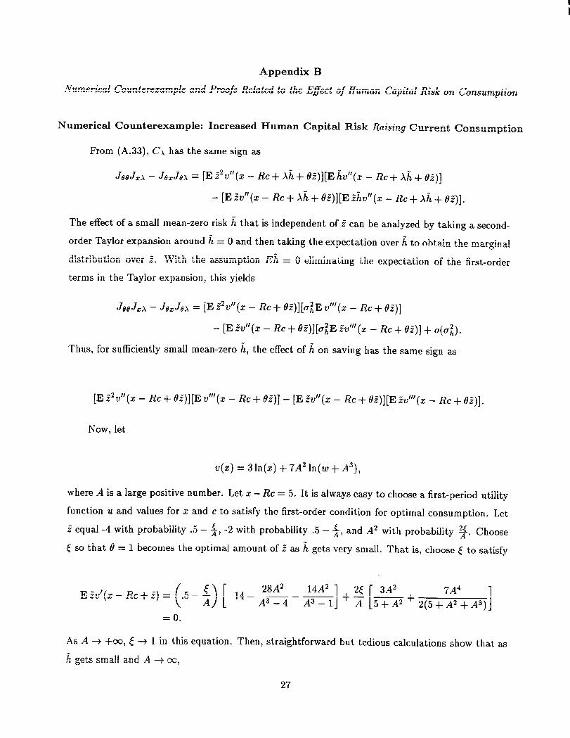
2AIndeed,the numefic~ Couterexamplein AppendixB involves only a three-point distribution for the fiaIICid

16

IV. A Numerical Illustration

Several of the results in the previous section indicate that the effect of human capital risk on

financial risk-taking can be substantial. Proposition 2 shows that this effect is at le=t as strong

as the effect of human capital risk on consumption, while Proposition 3 shows that the effect is

at le~t M strong as the effect of human capital risk on utility. Thus, these results imply that

changes in taxes that reduce labor income risk can have a noticeable effect on financial risk-taking.

To provide more direct evidence on the magnitude of this effect, we present the following simple

numerical illustration.

We interpret our model as a life-cycle model, with each period lasting one generation. Let the

utility function be

u–– .5[ln(c~) + Eln(tQ)],

set the real interest rate to zero, and normalize initial resources to 2. The factor of.5 on the utility

function means that a 1 percent increase in overall resources produces a .01 increase in utility. In

the absence of human capital risk and any financial risk-taking opportunities, the individual would

choose to consume 1 in each period, and would achieve a total utility of O.

Now introduce a financial risk-taking opportunity. Suppose that borrowing one unit to invest

in the risky asset has an equal chance of yielding .5 or -.25; that is, Z = .5 with probability one

half and -.25 with probability one-half. It is e~y to calculate that in the absence of any human

capital risk, the agent will continue

Consumption in the second period

will be .03.

to consume 1 in the first period and invest 1 in the risky asset.

will be 1.5 or .75 with equal probability, and expected utility

Finally, we add human capital risk, with a mean-zero symmetric two-point distribution, whose

standard deviation after taxes is (1 – ~)av. Table 1 shows optimal values of 0, c, and U for values

of (1 – ~)au between O and 1. Note that 0, c, and U are measured in comparable units, with

a difference of .01 representing the effect of a 1 percent change in

implication of our propositions that the effect of human capital risk

25

scale.25 Table 1 confirms the

on risky investment is greater

risk, a small mean-zero human capital risk, and a utility function that is the sum of two logarithmic utilitvfunctions with different origins, so there is not much room to strengthen Corollaries 4.1 an~ 4.2. Note th~ta utility function that is the sum of two logarithmic utility functions codd arise as a reduced form from anunderlying logarithmic utility function with a third backgroundrisk. Thus, there is no way to extend Corollary4.1 to allow for such a third (exogenous) risk. Corollary 4.2 can readily be extended to such a situation, sincethe financial risk wodd still have a two-point distribution, and decreasing absolute risk aversion is unalteredby a background risk.

This statement is always true for ~, and is true for Oand c when they are near 1. Taking logarithms of 8 andc would make the comparison more exact.

17

than its effect on consumption, which is in turn greater than its effect on utility.

(1 - T)o, e c u

o.1.2.3.4.5.6.7.8.9

1.0

11.99 .99.95 .98.89 .95.82 .92.75 .88.68 .84.61 .79.54 .74.48 .69.42 .63

.03

.03

.02

.00–.01–.04–.07–.10–.14–.19–.24

If the standard deviation of future labor income is .5 (within the range studied by Barsky,

Mankiw and Zeldes (1986)), then raising the future marginal tax rate from O to 20 percent causes

(1 - ~)oy to decline from .5 to .4. Table 1 shows that this 20 percentage point increase in the

tax rate produces close to a 10 percent increase in risky investment (from .75 to .82). Thus, the

semi-el~ticity of risky investment with respect to the future tax rate is roughly one-half. A 20

percentage point increase in the tax rate from 20 percent to 40 percent produces an 8 percent

increase in risky investment (from .82 to .89), for asemi-el~ticity of roughly two-fifths.

The size of this effect is sensitive to the amount ofhuman capital risk, ~one would expect.

If the standard deviation of future labor income is .4, for example, then an increase in the future

marginal tax rate from O to 25~0 produces an 8 percent increase in risky investment, for a semi-

el~ticity of roughly one-third. As human capital risk declines further, the semi-elasticity of risky

investment with respect to the tax rate declines as well.

There is also some direct empirical evidence that the effect ofhuman capital risk on financial

risk-taking can be substantial. Guise, Jappelli, and Terlizzese (1994) study the portfolio choices

of Italian households using the Survey of Income and Wealth. Their estimates suggest that the

elimination of income uncertainty would increase the portfolio share of risky assets by 2 to 14

percentage points (Tables 5 and 7).

V. Conclusion

Individuals’ ability to earn labor income is often their most valuable asset; but this =set

carries with it a large and mostly unmarketable risk. A decrease in current taxes combined with

an offsetting future increase in proportional or progressive labor income taxes provides insurance

18

against this risk. (And because most labor income risk is idiosyncratic, individual uncertainty can

be reduced with no increase in the uncertainty of government revenue.) Barsky, Mankiw and Zeldes

(1986) show that the reduction in idiosyncratic labor income risk acts through the precautionary

saving motive to reduce saving relative to a Ricardian benchmark. In this paper we show that the

reduction in idiosyncratic labor income risk affects portfolio decisions as well.

We analyze the effect of labor income risk on the joint saving/portfolio-composition decision

in a two-period model. We show that, given plausible restrictions on preferences, any change in

taxes that reduces an individual’s labor income risk and does not make her worse off will lead her

to invest more in a risky security, even if its return is statistically independent of the labor income

risk. A deferral of labor income taxes with no change in their expected present value is one such

tax change.

An additional curious result is that the effect of labor income risk on portfolio composition can

be so powerful that consequent indirect effects overturn the usual positive effect of labor income

risk on overall saving that is familiar from the precautionary saving literature. Ruling Out this

possibility requires relatively strict assumptions, such as constant relative risk aversion or a two-

point distribution for the return on the financial asset. This counterintuitive result turns out to be

related to the difficulty of guaranteeing that a pair of independent risks will both be normal goods.

One implication of our results concerns the effect of government debt issuance on risky invest-

ment. Suppose that the government reduces taxes today and raises taxes in the future, although

not necessarily by a corresponding amount. The results in Section III imply that this increase in

government debt will crowd in risky investment whenever any of the following conditions is satisfied:

(1) the expected present value of taxes faced by an individual is unchanged—i.e., there is a change

only in the timing of taxes (Corollary 3.1);

(2) the incre=ed future taxes have a strong enough insurance effect that the policy raises expected

utility (Proposition 3); or

(3) the tax changes lead to higher current consumption (Proposition 2).

Thus we concur with Friedman (1978) that crowding in will occur when the government reduces

taxes now and pays off the debt with higher taxes in the future.26 But our results are based on

26 ~~el (1985) estimates that pol-tfo~o effects on rates of return are very small, but that crowding in Of equity

investment is more likely than crowding out. We can foresee two ways in which an empirical analysis based onour approach would differ from Frankel’s. First, Frankel does not allow for the effects of future tax liabilities,which play an important role in our analysis. Second, Frankel constrains government debt to affect assetdemands only through changes in the market portfolio, and therefore through the covariances of asset returnswith the market portfolio. In our approach, the risk aversion of the indirect utility function depends on expectedfuture tax rates; therefore, changing those rates changes the market risk premium.

19

a neoclassical foundation of expected utility maximization in the absence of complete insurance

markets. Moreover, individuals in our model are fully aware of their future tax liabilities, which

allows us to show that financial crowding in can coexist with Ricardian equivalence of lumpsum

tax rescheduling.

Thus, our analysis establishes clear results about the effect of labor income risk on investment.

in other risky assets, 27 but Cwts some doubt on the generality of previous results about the effect

of labor income risk on total saving.28

27 It may be ~~rising that we Cm establish such clear results about labor income taxes and financial risk-taking

when the literature on capital income taxes and financial risk-taking is replete with ambiguities. The mainexplanation for the difference is that individuals cannot trade away their risky human capital in the way thatthey can trade away risky financial assets.

28 One ~rection for fmther rese~ch is to extend our restits to models with more than two periods. Kimball

(1990b) gives one idea of how this might be done. In a multiperiod model, the absolute risk aversion of thevalue function is equal to the product of the absolute risk aversion of the underlying period utility function andthe marginal propensity to consume out of wealth. Under conditions similar to those we assume, idiosyncraticlabor income risk raises the absolute risk aversion of the value function both by raising the marginal propensityto consume out of wealth and by raising the absolute risk aversion of the underlying period utility functionthrough lowering consumption. Equivalently, Breeden (1986) finds that for continuous-time diffusion processes,the expected rate of return differential between risky and riskless securities should be equal to the product of anagent’s underlying risk aversion and the covariance of the rate of return differential with consumption growth.Grossman and Shiner (1982) show that this relationship can be aggregated: the market risk premium shouldbe equal to the product of a weighted average of agents’ underlying risk aversions and the covariance betweenthe rate of return differential and aggregate consumption growth. Idiosyncratic labor income risk raises thepremium for holding risky assets in two ways: by lowering consumption, and therefore underlying risk aversion,and by raising the marginal propensity to consume out of wealth and therefore the covariance of consumptionwith the returns on risky securities in which agents have substantial positions.

20

Appendh A

Proojs of Propositions 1-3

Five lemmas prepare the ground for proofs of Propositions 1–3. Define

J(c, e; x, A) = u(c) + E V(Z– Rc + Ak + 6Z). (Al)

Then

(c(z, A),e(z, A)) = arg ~~x J(c, 0; z, A). (A.2)?

Lemm~ 1–5 characterize the function J. All of the results here assume that the risks 2 and ~ are

nondegenerate and statistically independent of each other and that u’(0) >0, U“(O)<0, v’(”) >0,.

~“(.) < 0“ Lemmas 3 and 4 relY in addition On v having decre=ing absolute risk aversion. Lemma

5 relies on v having decreasing absolute prudence, but does not rely on decre~ing absolute risk

aversion. Subscripts denote partial derivatives.

Lemma 1: For all c, d, z and A,

and

Jcc(c, e; x, A) = R2JZZ(C,6; X, ~) + U“(C),

Jcd(c, e; z, A) = –RJ=6 (C,6; X, ~) ,

JCZ(C,6; z, A) = –RJZ=(C, 0; X, ~),

J.}(C, 0; x, A) = –RJr~ (C,6; z, ~),

JOg<0

Proof. Differentiate (A.1).~

Lemma 2: For all c, 0, x and A,

JCCJd8– J~d > R2[JZzJ6e – JjZ] >0,

(A.3)

(A.4)

(A.5)

(A.6)

(A.7)

(A.8)

(A.9)

(A.1O)

(All)

and

(A.12)

Proof. Any sum of concave functions and any expectation over concave functions is concave. Since

both u and v are jointly concave in all c, 0, x, A for particular realizations of 2 and fi, the function

J is jointly concave in all four arguments. The strict inequalities follow from U“(C)<0, v“(”) <0,

(A.7), (A.8) and from the nondegeneracy and independence of 2 and i.2g=

Lemma 3: For any random variable ~, the derived utility function

inherits

Proof.

(A.13)O(z) = E V(2 + ~)

decreasing absolute risk aversion from v.

Both Nachman (1982) and Kihlstrom, Romer and Williams (1981) give proofs of Lemma

3. Since decre~ing absolute risk aversion is equivalent to convexity of ln(v’(z)), Lemma 3 is a

consequence of Artin’s 1931 Theorem that log-convexity is preserved under expectations. Marshall

and Olkin (1979) give a particularly simple proof of Artin’s theorem based on the fact that any sum

of or expectation over positive semidefinite matrices is positive semidefinite. Decreasing absolute

risk aversion of v implies convexity of in (v’(z + ~)) for each realization of ~, which is equivalent to

positive semidefiniteness of the matrix

[

V’(Z+ ~) V’(X+ ~ + 6)

1U’(Z+ j +6) U’(Z+ q + 26) “

This implies positive definiteness of

[

E VI(Z+ ~) E V’(X+ j + 6)

Ev’(x + ~+~) Ev’(z+ Q+ 2d) 1

and decreasing absolute risk aversion for 0(’) .-

Lemma 4: If O ~ O, then J8Z(C,6; x, ~) ~ O wherever Jo(c, O;x, A) ~ O. Similarly, if A ~ O, then

J~Z(c, 0;x, A) ~ O wherever J~(c, 6; x, ~) ~ O.

Proof. By the symmetry between 8 and ~ in the definition of J (Al), proving one half of Lemma

4 is enough to prove both halves. Letting @= Afi– Rc in (A.13),

~o(c, 6; x, ~) = E ZV’(X– Rc+ 62 + ~k) = E ~ti’(X+ 8:) (A.16)

(A.14)

(A.15)

29 The Cauchy-Schw=tz inequalities which apply to the expanded versions of (A.g–A. 12) hold with equalitY o~Y

when the random variables are perfectly correlated or when one of the random variables is degenerate.

22

and

J8Z(C,9;z, A) = E ZV”(Z – Rc + e: + ~k)

because of the independence of 2 and ~. Decreasing absolute

increasing function of 2, so thatO“(X+ 8Z) o“(x)0’(2 + 02) – ti~(z)

has the same sign m 2. Thus,

Je (c, e; x, A) = E ZO’(Z+ 0;)

implies

= E ZO”(z + 02) (A.17)

risk aversion of O makes O“(Z+8Z)an0’(Z+6Z)

(A.18)

(A.19)

Lemma 5: For any c, Z, 6 ~ O and A ~ O,

J8J(c,e;z,A)JCZ(C,0;x,A) – J@z(c,e;z,A)JAZ(C,6;x,A) ~ o (A.20)

Proof. Decreasing absolute prudence is equivalent to convexity of ln(–v”). Therefore, for any four

quantities Z1, 22, hl and h2,

ln(–v’’(z+Ozl +Ahl)) +ln(-v’’(z+8z2 +Ah2)) ~ ln(–v’’(x+Ozl +Ah2)) +ln(–v’’(z+Oz2 +Ah1))

(A.21)

when (Z2– Z1) (h2 – hl) z O, with the direction of the inequality in (A.21) reversed when

(22 —z1)(h2 – hl) ~ O. Exponentiating both sides of (A.21) and subtracting, the quantity

always has the same sign as (Z2– Z1) (h2 – hi). Thus, if 21, :2, 11 and ~2 are mutually independent

random variables with il and 22 having the same distribution as 5, and kl and fi2 having the same

distribution M fi, then

23

I

Je~(c, e;x, A)JZZ(C,e;x, A)– Jdz(c, e;x, A)JAZ(C,e;x, A)

= {E2iv”(z + 85 + Ai)}{E V“(X + 82 + ~k)}

- {E ZV”(X+ 82 + At)}{E kV”(Z + 8Z + ~fi)}

1=zE(Z2– Z1)(h2– L~)[vfl(z +ez~+Ail)v”(z+ez2 +Atz)

–v’’(z+ ezl+Ak2)v”(z +dE2+Ai~)]

~o.m

Remark: Ifv exhibits increasing absolute prudence over the interval of interest, essentially the

same proof can be used to show that Je~JZZ –JoZJ~Z <0. This converse to Lemma 5 allows one

to establish the converseto Proposition 2.~

Proofof Proposition 1

The a,gent’s problem can be rewritten as

~~x J(c, e;2,A).?

The first-order conditions are

Jc(c(z, A),e(x,A);x,A)= o (A.24)

J@(c(x, A),e(z,A);x,A) =0 (A25)

Differentiating (A.24) and (A.25) with respect to xand~ and arranging the resultsin matrix form

and

Define

A=

Then by Lemma 1,

J. . J.@

1JCe Joe “

A-l = 1

[

Jg8 –JC6JCCJ4d-J:. -Jce J.. 1

[

~-~ JotI RJ6.=1RJeZ R2JZZ+U” ‘

(A.22)

(A.23)

(A.26)

(A.27)

(A.28)

24

where

A = JCCJ6e– J:a >0 (A.29)

by Lemma 2. Multiplying both sides of (A.26) on the left by A-l and restricting our attention for

now to the left column of the result,

[::l=-A-l[~i:l(A.30)

–A-l[

Jee=‘J’” ,,1 [-::”1RJ8Z R2JZZ+ U

[

= A-l R(JeeJZZ – JjZ)– u“Jez 1

●

The effect of wealth on c given by Cz is positive by Lemma 2. The effect of wealth on O given by

@Zis positive by Lemma 4, in conjunction with the first-order condition (A.25).~

Proof of Proposition 2

Since the determinant of the product of two matrices is equal to the product of the determi-

nants, (A.26) implies

and therefore

>—

~[J JA

8A .Z – Je=JJZ]

o,

(A.31)

(A.32)

by Lemma 1, Lemma 5 and (A.29).,

Remark: As noted in the remark to Lemma 5, incre~ing absolute prudence on any interval

implies that Je~JZZ– J6ZJ~Z<0, and therefore that C~@Z– CZQ~ ~ O. Since it is always possible

to choose z, ~ and At in such a way that only the values of v on a small interval matter, decreasing

absolute prudence is a necessary condition for (A.32) to hold for any x, 5 and ~~.~

Proof of Proposition 3

Calculating CJ and ~~ just as we calculated Cz and ~z (that is, by multiplying both sides of

A.26 on the left by A-l),

[:tl=-A-l[~:l(A.33)

25

= –A-l

[

Jge

‘J” 1[-:’”’1RJo. R2JZZ+ U!’

~_l

[

R(JeeJxJ – JeZJg~)=1R2(J$ZJZ~– Jz=Je~)– u“Je~ “

Lemma 5 implies that R2(J@ZJz~– JzZJg~) <0. Moreover, since J.x <0, Lemma 5 implies that

The first-order condition Je = O, together with Lemma 4, implies that Je. ~ O, and the assumption

of Proposition 3 that J~ < 0, together with Lemma 4, implies that J~Z ~ O. Therefore, (A.34)

guarantees thatu“JO=J~Z

-u’’Je~ < –J

<0. (A.35)xx

26

Numerical

Numerical

Appendix B

Counterezample and Proofs Related to the Eflect of Human C’apitalRisk on Consumption

Counterexample: Increased Human Capital Risk Raising Current Consumption

k’rom (A.33), CA h~ the same sign w

JoeJZ~ – JeZJe~ = [E ~2V”(z – Rc

- [E ZV”(Z-

The effect of a small mean-zero risk k that is

+ ~k+ OZ)][EfiV”(Z– Rc + Ah + 02)]

~c + ~fi+ 82)][E ~kV”(Z – Rc + ~k + 0:)].

independent of 2 can be analyzed by taking a second-

order Taylor expansion around ~ = Oand then taking the expectation over ~ to obtain the marginal

distribution over 2. With the ~sumption Eh = O eliminating the expectation of the first-order

terms in the Taylor expansion, this yields

J8@JZ~– JeZJ8~= [E Z2V”(X- Rc + OZ)][o~Ev’”(Z - RC + 8z)]

- [E ~V”(Z - Rc + 02)][o;E ~V’”(Z– Rc + 82)]+ O(C7:).

Thus, for sufficiently small mean-zero ~, the effect of ~ on saving has the same sign as

[E ~2V”(Z – Rc + 8z)][E U’”(Z– Rc + 82)] – [E ZV”(Z– Rc + 02)][E~V’”(Z– Rc + 02)].

Now, let

v(x) = 31n(z) + 7A2 ln(w + A3),

where A is a large positive number. Let x – Rc = 5. It is always easy to choose a first-period utility

function u and values for x and c to satisfy the first-order condition for optimal consumption. Let

2 equal -4 with probability .5 – ~, -2 with probability .5 – ~, and A2 with probability ~. Choose

~ so that O= 1 becomes the optimal amount of 2 w h gets very small. That is, choose f to satisfy

As A ~ +00, ~ ~ 1 in this equation. Then, straightforward but tedious calculations show that as

~ gets small and A ~ m,

27

I

EZ2V’’(.)E V’’’(.) – E5v’’(.)EZV’’’(.) = ; >0.

Thus, if k gets small enough and A gets big enough, CA becomes positive.

positive, adding a positive constant to the mean-zero human

strongly positive. ■

Proof of Proposition

From (A.33),

sign (C~(x, A)) = sign(~~~~=~ –

If A were chosen optimally, the first-order condition

JA(C,e; x, A) = o

capital risk ~ can

4

Since C. is always

only make CA more

(B.1)

(B.2)

would always hold. All three of the variables c, 8 and J would be functions of x alone. Differentiating

(B.2) and the other two first-order conditions with respect to x would yield the matrix equation

Define

By Cramer’s rule,

d~” –1 ‘cc ‘Ce ‘=xJCe J$e JOZ

dx = det(B) JC~ Je~ JAx

(B.4)

(B.5)

where the second line results from subtracting R times the third column from the first column of

the determinant in the numerator on the first line. Since B is a negative definite 3 x 3 matrix,

det(B) <0 and

(-)

d~”.‘tgn dx =

–sign(JOe J~Z – Je~J6z) = –sign(C’~).,

28

Proof of Corollary 4.1

If

and

and

(B.7)

(B.8)

(B.9)

(B.1O)

Therefore, if they were both freely chosen, the optimal values of A and Owould be proportional to

z – Rc – Zo, guaranteeing that both would increase with x.=

Proof of Corollary 4.2

By (A.33), in order to prove the corollary, we must show that

Je8J$J – JeZJg~ <0

when z has a two point distribution. Given the fact that Jee < 0, this is equivalent to

where

(B.11)

d6 JeZ— = ——dx Jee

(B.12)

is the optimal adjustment in 8 when x changes with A remaining fixed. With ~ held fixed, AL is a

fixed background risk, and the decre~ing absolute risk aversion of v is enough to guarantee that

M > ().dz —

Denote the two possible realizations of 2 as Zl, which occurs with probability p, and 22, which

occurs with probability (1 – p). Then, the equation Je = O, which characterizes an optimal value

of 0, becomes

29

pzlE [v’(z – Rc + d~l + At)]+ (1 – p)z2E [v’(z – Rc + 622+ Afi)]= O, (B.13)

where the expectations denoted by E here are only over h. (Note the use of independence between

Z and k in expanding out the expectation over

opposite signs. Without loss of generality, let 22

Taking the derivative of (B.13) with respect

condition, yields

2.) Clearly, (B.13) requires Z1 and 22 to be of

>0>21.

to Z, with Oadjusting to maintain this first-order

‘zl(l+z’:)E’v’’(x-‘c+’zl+Ak)l+(l-p)z2(1+z2:)E’v’’(z-Rc+’z2+Ai)l=(B.14)

Since Z2 >0> z1, equation (B.14) implies that both (1 + zz~) and (1 + 21~) are of the same

sign and therefore both positive.

Turning to the quantity of interest, (B.11) can be expanded to

“z+J’’:=p(l+zl:)E~v’’Rcsezl+A’)l’)l (B.15)

‘(1-p) (1+z2:)E’iv’’(z-Rc+ ez2+Ai)’~o

Dividing (B.15) by the negative quantity

-PZ1(l+Z1:)''v''(2-Rc+`z'+Ak)l=(1-p'(1+z2:)E'v''(z-Rc+ezAi)l1(B.15) becomes

1 E [kV”(Z – Rc+ 8ZI + Ai)] + 1 E[~v”(z – Rc+ 022 + ~t)] <

(-z1) E[v”(z – Rc + Ozl + AL)] ~ E [v~l(~– Rc+ 8ZZ+ AL)] -

In order to prove (B.16), use the stipulation that at the point in question,

expanded form,

pE ~V’(Z – RC + 8Z~ + ~k) + (1– p)E kV’(Z – RC + 622 i-~k) = 0.

Dividing (B.17) by the positive quantity

o (B.16)

JA ~ O, or in

(B.17)

30

–pzl E [v’(z – Rc + Ozl + Ak)] = (1– p)E [v’(z – Rc + ez2 + AL)],

(B.17) becomes

1 E [iv’(z – Bc+ Ozl+ Ak)] + 1 E [kv’(z – Rc+ 8Z2+ ~~)]

(-ZI) E[v’(x - Rc+8.z, + AZ)]<0.; E IvI(Z– Rc + Ozz + AA)]

(B.18)

Note that except for involving the first derivative of v instead of the second, (B.18) is of the same

form as (B.16), which needs to be proven.

To prove (B.16) from (B.18), we will show that each of the two terms in (B.16) is less than or

equal to the corresponding term in (B.16). For z = 1,2, define

E[kV”(2– RC + Ozi+ AL)]~i=

E[v”(X – Rc+ Ozi + Ak)] “(B.19)

Decreasing absolute risk aversion, which guarantees that –v” falls faster than v’ in proportional

terms, implies that for any scalar realization h of the random variable k,

Taking expectations of both sides of (B.20) over random ~,

E [hV”(X – RC + 6~i+ ~k)] – ~iE [V”(2– RC + dzi + Jk)]

v“(X – RC+ Ozi + Aqi)

(B.20)

(B.21)

But, by the definition of vi, the right-hand side of (B.21) is less than or equal to zero. Thus, the

left-hand side of (B.21) is also less than or equal to zero, implying

Therefore, (B.18) implies (B.16).=

Intuitively, the key to the proof is that with a twmpoint distribution for z, an increase in x

with its consequent increase in 8 leads to an increase in z — RC + Ozi for both ~ = 1 and ~ = 2.

This incre~e in x – Rc + Ozi leads to an incre~e in the marginal benefit of higher A relative to

the expected marginal utility v’ for both i = 1 and i = 2. Since the condition for optimal Oinsures

that the importance of expected marginal utility for i = 1 and z = 2 is in a fixed ratio, this leads

to an increase in the overall marginal benefit of A.

31

References

Ahsan, Syed M., “Taxation in a Two-Period Temporal Model of Consumption and Portfolio Allo-

cation,” Journal of Public Economics, 5 (April-May, 1976), 337-352.

Auerbach, Alan J. and Laurence J. Kotlikoff, Dynamic FiscaZ PoZicy (Cambridge: Cambridge

University Press, 1987).

13arro, Robert J., “Are Government Bonds Net Wealth?” Journal of Political Economy 82 (Novem-

ber/December, 1974), 1095-1117.

Barsky, Robert B., N. Gregory Mankiw, and Stephen P. Zeldes, “Ricardian Consumers with Key-

nesian Propensities,” American Economic Review, 76 (September, 1986), 676-691.

Bodie, Zvi, Robert C. ~Merton,and William F. Samuelson, “Labor Supply Flexibility and Portfolio

Choice in a Life-Cycle Model,” Journal of Economic Dynamics and Control, 16 (July-October,

1992), 427-449.

Breeden, Dougl~ T., “Consumption, Production, Inflation and Interest Rates: A Synthesis,” Jour-

nal of Financial Economics, 16 (May, 1986), 3-39.

Caballero, Ricardo, “Consumption Puzzles and Precautionary Savings,” Journal of Monetary Eco.

nomics, 24 (January, 1990), 113–136.

Chan, Louis Kuo Chi, “Uncertainty and Neutrality of Government Financing Policy,” Journal of

Monetary Economics 11 (May, 1983): 351-372.

Davies, James and John Whalley, “Taxes and Capital Formation: How Important is Human Cap-

ital?” ch. 6 in lvational Saving and Economic Performance, B. Douglas Bernheim and John

B. Shoven, eds. (Chicago: University of Chicago Press, 1991).

Devereux, Michael B., and Gregor W. Smith, “International Risk Sharing and Economic Growth,”

International Economic Review 35 (August, 1994), 535-550.

Domar, Evsey D. and Richard A. Musgrave, “Proportional Income Taxation and Risk-Taking,)’

Quarterly Journal of Economics 58 (May, 1944), 388-422.

Dr&ze, Jacques H., and Franco Modigliani, “Consumption Decisions Under Uncertainty,” Journal

of Economic Theory, 5 (December, 1972), 308–335.

Driffill, E. J. and Harvey S. Rosen, “Taxation and Excess Burden: A Life-Cycle Perspective,”

International Economic Review, 24 (October, 1983), 671-683.

Easley, David, Nicholas M. Kiefer, and Uri M. Possen, “An Equilibrium Analysis of Fiscal Policy

with Uncertainty and Incomplete Markets,” International Economic Review, 34 (November,

1993), 935-952.

32

Eaton, Jonathan, and Harvey S. Rosen, “Taxation, Human Capital, and Uncertainty,” American

Economic Review, 70 (September, 1980), 705-715.

Economic Report of the President (Washington, D.C., 1996).

Feldstein, Martin, “The Effects of Taxation on Risk Taking,” Journal of Political Economy, 77

(Sept.-oct. 1969), 755-764.

Feldstein, Martin, Capital Taxation (Cambridge: Harvard University Press, 1983).

Feldstein, Martin, “The Optimal Level of Social Security Benefits,” QuarterZy Journal of Eco.

nomics, 100 (May, 1985), 303–320.

Frankel, Jeffrey A., “Portfolio Crowding-Out, Empirically Estimated,” Quarter/y JournaZ of Eco-

nomics, 100 (August, 1985), 1041–1066.

Friedman, Benjamin M., “Crowding Out or Crowding In? Economic Consequences of Financing

Government Deficits,” Brvokings Papers on Economic Activity, 3:1978, 593-641.

Friend, Irwin, and Marshall E. Blume, “The Demand for Risky Assets,” American Economic Re-

view, 65 (December, 1975), 900–922.

Grossman, Sanford J., and Robert J. Shiner, “Consumption Correlatedness and Risk Measurement

in Economies with Non-Traded Assets and Heterogeneous Information,” Journa/ of Financial

Economics, 10 (July, 1982), 195-210.

Guise, Luigi, Tullio Jappelli and Daniele Terlizzese, “Income Risk, Borrowing Constraints and

Portfolio Choicel” CEPR Discussion Paper # 888 (January, 1994).

Hart, Oliver E., “Some Negative Results on the Existence of Comparative Statics Results in Port-

folio Theory,” Review of Economic Studies, 42 (October, 1975), 615-621.

Jaffe, Adam B., “Technological Opportunity and Spillovers of R & D,” American Economic Review,

76 (December, 1986), 984-1001.

Kanbur, S. M., “Risk Taking and Taxation: An

nomics, 15 (April, 1981), 163–184.

Kaplow, Louis, “A Note on Taxation as Social

Working Paper # 3708 (May, 1991).

Alternative Perspective,” Journal of Public ECO-

Insurance for Uncertain Labor Income,” NBER

Kihlstrom, Richard E., David Romer, and Steve Williams, “Risk Aversion with Random Initial

Wealth,” Econometric, 44 (June, 1981), 911-920.

Kimball, Miles S., “Precautionary Saving in the Small and in the Large,” Econometric, 58 (Jan-

uary 1990a), 53–73.

Kimball, Miles S., “Precautionary Saving and the Marginal Propensity to Consume,” NBER Work-

33

ing Paper # 3403 (1990b).

Kimball, Miles S., “Standard Risk Aversion,” Econometric, 61 (May, 1993), 589-611.

Kimball, Miles S., “Precautionary Motives for Holding Assets,” The New Palgrave D~ct~onary of

Money and Finance, Peter Newman, Murray Milgate and John Eatwell, eds. (1992), Stockton

Press, New York: 158-161.

Kimball, Miles S., and N. Gregory Mankiw, “Precautionary Saving and the Timing of Taxes,”

Journal of Political Economy, 97 (August, 1989): 863-879.

Kimball, Miles S., and Phillipe Weil, “Precautionary Saving and Consumption Smoothing over

Time and Possibilities,” NBER Working Paper # 3976 (1992).

Leland, Hayne E., “Saving and Uncertainty: The Precautionary Demand for Saving,” Quarterly

Journal of Economics, 82 (August, 1968), 465-473.

MmDonald, Glenn M., “The Economics of Rising Stars,” American Economic Review, 78 (March,

1988), 155-166.

Marshall, Albert W. and Ingram Olkin, Inequalities: Theory of Majorization and its Applications

(New York: Academic Press, 1979).

Merton, Robert C., “On the Role of Social Security as a Means for Efficient Risk Sharing in an

Economy Where Human Capital Is Not Tradable,” Financial Aspects of the United States

Pension System, Zvi Bodie and John Shoven, eds. (Chicago: University of Chicago Press,

1983).

Nachman, David C., “Preservation of ‘More Risk Averse’ Under Expectations,” Journal of ECO-

nomic Theory, 28 (December, 1982), 361–368.

Pratt, John W., “Risk Aversion in the Small and in the Large,” Econometric, 32 (January-April,

1964), 122-137.

Pratt, John W., and Richard J. Zeckhauser, “Proper Risk Aversion,” Econometrica, 60 (January,

1987), 143-154.

Rothschild, Michael and Joseph E. Stiglitz, “Increasing Risk II: Its Economic Consequences,” Jour-

nal of Economic Theory 3 (March, 1971), 66–84.

Sandmo, Agnar, “Capital Risk, Consumption, and Portfolio Choice,” Econometric, 37 (October,

1969), 586-599.

Sandmo, Agnar, “The Effect of Uncertainty on Saving Decisions,” Review of Economic studies, 37

(July, 1970), 353-360.

Sandmo, Agnar, “The Effects of Taxation on Savings and Risk Taking,” Handbook of Public ECO-

34

nomics, A. J. Auerbach and M. Feldstein, eds. (Amsterdam: North-Holland, 1985).

Shleifer, Andrei and Robert W. Vishny, “The Efficiency of Investment in the Presence of Aggregate

Demand Spillovers,” Journal of Political Economy 96 (December, 1988), 1221-1231.

Skinner, Jonathan, “Risky Income, Life Cycle Consumption, and Precautionary Savings,” JournaZ

of Monetary Economics, 22 (September, 1988), 237–255.

Varian, Hal R., “Redistributive Taxation as Social Insurance,” Journal of Public Economics, 14

(August, 1980), 49-68.

Weil, Philippe, “Precautionary Savings and the Permanent Income Hypothesis,” Review of Eco-

nomic Studies, 60 (April, 1993),367–383.

Zeldes, Stephen P., “Optimal Consumption with Stochastic Income: Deviations from Certainty

Equivalence,” Quarterly Journal of Economics, 104 (1989), 275-298.

35

i

(C(x,ko),e(x,ko))

C(X,A1),@(x,A*))

(cx,@x)

c

Figure 1