DISCUSSION PAPER SERIES Forschungsinstitut zur Zukunft der Arbeit Institute for the Study of Labor Taxation and the Long Run Allocation of Labor: Theory and Danish Evidence IZA DP No. 8246 June 2014 Claus Thustrup Kreiner Jakob Roland Munch Hans Jørgen Whitta-Jacobsen
Transcript
DI
SC
US
SI
ON
P
AP
ER
S
ER
IE
S
Forschungsinstitut zur Zukunft der ArbeitInstitute for the Study of Labor
Taxation and the Long Run Allocation of Labor: Theory and Danish Evidence
IZA DP No. 8246
June 2014
Claus Thustrup KreinerJakob Roland MunchHans Jørgen Whitta-Jacobsen
Taxation and the Long Run Allocation of Labor: Theory and Danish Evidence
Claus Thustrup Kreiner University of Copenhagen,
CESifo and CEPR
Jakob Roland Munch University of Copenhagen
and IZA
Hans Jørgen Whitta-Jacobsen University of Copenhagen
Any opinions expressed here are those of the author(s) and not those of IZA. Research published in this series may include views on policy, but the institute itself takes no institutional policy positions. The IZA research network is committed to the IZA Guiding Principles of Research Integrity. The Institute for the Study of Labor (IZA) in Bonn is a local and virtual international research center and a place of communication between science, politics and business. IZA is an independent nonprofit organization supported by Deutsche Post Foundation. The center is associated with the University of Bonn and offers a stimulating research environment through its international network, workshops and conferences, data service, project support, research visits and doctoral program. IZA engages in (i) original and internationally competitive research in all fields of labor economics, (ii) development of policy concepts, and (iii) dissemination of research results and concepts to the interested public. IZA Discussion Papers often represent preliminary work and are circulated to encourage discussion. Citation of such a paper should account for its provisional character. A revised version may be available directly from the author.
Taxation and the Long Run Allocation of Labor: Theory and Danish Evidence*
Inspired by Hayek (1945), we study the distortionary effects of taxation on labor mobility and the long run allocation of labor across different profitable opportunities. These effects are not well detected by the methods applied in the large public finance literature estimating the elasticity of taxable income and quantifying the efficiency loss from taxation. Our analysis builds on a standard search theoretic framework where workers are continually seeking better paid jobs, but are also fired from time to time because of economic development and productivity shocks. We incorporate non-linear taxation into this setting and estimate the structural parameters of the model using employer-employee register based data for the full Danish population of workers and workplaces for the years 2004-2006. Our results indicate that along the intensive margin the Danish taxation generates an overall efficiency loss corresponding to a 12 percent reduction in total income. It is possible to reap 4/5 of this potential efficiency gain by going from a high-tax Scandinavian system to a level of taxation in line with low-tax OECD countries such as the United States. The tax-responsiveness of labor mobility and allocation corresponds to an elasticity of taxable income with respect to the net-of-tax rate in the range 0.15-0.35. JEL Classification: J62, H24 Keywords: tax distortions, labor mobility, elasticity of taxable income Corresponding author: Jakob Roland Munch Department of Economics University of Copenhagen Øster Farimagsgade 5 Building 26 1455 Copenhagen K Denmark E-mail: [email protected]
* We thank participants at the Conference on the Economics of the Nordic Model in Oslo for helpful comments and suggestions. Financial support from the Economic Policy Research Network (EPRN) is gratefully acknowledged.
Hayek (1945) argues convincingly that the true merit of the capitalist market economy is its capa-
bility of continually responding to the ongoing changes in needs and possibilities by reallocating
resources towards their best use.1 Prices convey information about productivity and scarcity of
resources, and owners of resources react on price signals to obtain the highest possible returns,
thereby collectively acting as an effective allocation device. According to this view, taxation dis-
torts the functioning of the market economy by creating a wedge between the private return and
the social return to a reallocation of resources, leaving socially desirable opportunities unexploited
as a result. This type of tax distortion should be relevant for the labor market since employees
change jobs many times during their career and economic incentives are a key determinant behind
job changing decisions (Topel and Ward, 1992).
This paper studies the impact of taxation on the mobility and allocation of labor, and quanti-
fies the effi ciency loss from misallocation of labor caused by taxation.2 As will be explained below,
labor mobility responses are fundamentally different from the hours-of-work responses of the basic
labor supply model, which underlies the modern reduced-form empirical identification methods to
measure behavioral responses to taxation. These methods are not well suited to detect mobility
behavior, and therefore we apply a structural approach. Our analysis builds on a standard search
theoretic framework, along the lines of Burdett (1978) and Christensen et al. (2005), where work-
ers continually seek better paid jobs, but are also fired from time to time because of economic
development and productivity shocks. We incorporate non-linear taxation into this setting and es-
timate the structural parameters of the model using employer-employee register based data for the
full Danish population of workers and workplaces for the years 2004-2006. The estimated model
is then used to examine the impact of different changes in the tax system, thereby characterizing
the distortionary effects of taxation on the allocation of labor.
The overall tax distortion is identified by an experiment where all taxation along the intensive
margin is replaced by lump sum taxation. For Denmark, with marginal tax rates ranging from
59 to 72 percent, the result is an increase in aggregate labor income of 1/4, and an effi ciency
gain equal to 12 percent of initial income. This is a sizable, although not huge, effi ciency loss,
which should be balanced against the (non-measured) gains in social welfare from social insurance
and equality achieved through high marginal taxation. Interestingly, it is possible to reap a very
large part of the potential effi ciency gain by going “half the way”and replace the current taxation
1The seminal article by Hayek was selected in 2011 to be one of the twenty most influential articles publishedby the American Economic Review in the entire history of the review.
2Our focus is on measuring behavioral responses to taxation and quantifying the effi ciency loss from taxation.This is in line with the literature estimating the elasticity of taxable income. We do not attempt to quantify thetrade-off between equality and effi ciency (see Immervoll et al, 2007), but a normative tax analysis should, of course,balance the effi ciency loss from taxation against the distributional consequences.
1
with a flat tax rate of 30 percent on all income. This shift from a Scandinavian tax system
with high marginal tax rates to a level of taxation in line with low-tax OECD countries such as
the United States increases total income by 20 percent and yields an effi ciency gain measured
in proportion to initial income of 10 percent. The large effect on economic effi ciency from going
only “half the way”reflects the well-known result in the economics of taxation that the marginal
effi ciency loss is growing in the level of taxation. The structural approach enables us to derive
this relationship between the marginal effi ciency loss and the level of taxation, which turns out to
be strongly convex with a Laffer rate around 2/3. Finally, and most importantly, we compute the
marginal tax distortion at the initial tax system and the elasticity of taxable income by looking
at a small reduction in all marginal tax rates.3 The marginal effi ciency effect is in this case equal
to 87 percent of the (mechanical) loss in tax revenue,4 which translates into an elasticity of labor
market income (taxable income) with respect to the net-of-tax rate of 0.3. A number of sensitivity
tests suggest that the estimate of the elasticity of taxable income due to mobility responses lies
in the interval 0.15 to 0.35.
Our results are related to the large public finance literature, recently surveyed by Saez et al.
(2012), estimating the elasticity of taxable income with respect to the net-of-tax rate using tax
return data. The ultimate goal of this literature is to estimate the ‘true’underlying structural
elasticity relevant for quantifying the effi ciency losses from taxation. In two influential papers,
Feldstein (1995, 1999) argued that the effects of the tax system on the reported income of the
tax payers capture all relevant effi ciency losses, and therefore the elasticity of taxable income is a
suffi cient statistic to compute the total tax distortion. However, the inclusion of taxable income
responses due to tax avoidance and evasion behavior relies on strong assumptions (Chetty, 2009;
Slemrod and Kopczuk, 2002), and recent empirical studies have increasingly focused on more
narrow income concepts, mainly labor income as we also do, in order to isolate real responses (e.g.
Chetty et al., 2011a; Kleven and Schultz, 2013).
Most of the literature has exploited variation in tax rates generated by tax reforms to iden-
tify the elasticity using difference-in-difference type methodologies where individual post-reform
income levels are compared to pre-reform levels. Saez et al. (2012) conclude that an elasticity of
taxable income of 0.25 seems to be a reasonable estimate from the existing studies and the recent
empirical evidence for Denmark in Kleven and Schultz (2013), based on a series of tax reforms and
a very rich administrative data set covering the entire Danish population, points to an elasticity
of labor income around 0.1.3More specifically, we consider a one percent increase in the net-of-tax rates.4This also implies that the degree of self-financing, which measures the share of the mechanical tax revenue
loss recouped by behavioral responses, equals 87 percent. For marginal reductions in taxation, the degree ofself-financing is equal to the effi ciency effect in proportion to the mechanical revenue change.
2
Other recent studies have exploited bunching at the kink points of the tax system to identify
the elasticity of taxable income (Saez, 2010; Chetty et al., 2011a, Bastani and Selin, 2014) and
have found very small elasticities. Using Danish data, Chetty et al. (2011a) estimate an elasticity
below 0.02. However, an important conclusion from this study is that the elasticity is larger when
measured at larger kinks in the tax schedule. This strongly indicates that labor supply decision
making is subject to short term frictions and adjustment costs, implying that the micro econo-
metric identification methods in general underestimate the structural elasticity. After accounting
for small frictions, corresponding to less than one percent of earnings, Chetty et al. (2011a,b) and
Chetty (2012) conclude that the small elasticities obtained in the micro labor supply literature
correspond to a structural intensive margin elasticity of around 0.3, more in line with the elasticity
found in the macro literature based on cross-country evidence.
Both the difference-in-difference type methods and the bunching method are unlikely to identify
the labor allocation effects of taxation studied here. To see why, consider a change of the tax system
where first all marginal tax rates are identical and then the marginal tax rates for income levels
above a certain threshold are raised to a new, higher level, thus introducing tax progressivity
with a kink-point in the tax schedule. According to a standard, hours-of-work labor supply model
with heterogeneity in abilities, the behavior of workers with income below the threshold will be
unaffected, while all workers with income above the threshold will reduce labor supply and income.
Hence, it is possible to separate workers into distinct control and treatment groups depending on
income levels before the tax change, and the tax increase makes workers pile up at the income level
of the kink-point, thereby creating a discontinuity in the density function. This makes it possible
to identify the underlying structural labor supply elasticity by measuring changes in income of the
treatment group relative to the control group or by exploiting the bunching of individuals at the
kink-point. In the search framework, both workers with income above the threshold and below it
will reduce search effort. The reason that also workers below the threshold reduce effort is that
their expected after-tax income gain from searching and climbing up the income ladder is reduced.
Therefore, they do not constitute a well-defined control group and the kink in the tax schedule
does not create an excess mass of individuals at the income threshold.5
To conclude, the otherwise strong empirical identification strategies normally used to identify
income responses to taxation and the elasticity of taxable income are not well-suited to detect the
income responses due to job mobility effects, and our estimates of the elasticity of taxable income
and of the tax distortions of labor allocation, based on a structural approach, indicate that these
job mobility effects are of a substantial magnitude.
5Another reason why the difference-in-difference types techniques are unlikely to detect the effects on searchbehavior is that job shifts and reallocation of labor are time-consuming processes, implying that it takes relativelylong time for the economy to reach its new long run distribution of earnings after a tax reform.
3
A few studies have analyzed the impact of taxation on job mobility decisions by looking at
the mobility of people across states (Feldstein and Wrobel, 1998) and across countries (Kleven et
al., 2014). The second study examines the impact of changes in the preferential tax regime for
foreign researchers and high-income foreigners in Denmark and finds large effects on the number
of highly paid foreigners. These types of studies are not comparable to our analysis of the impact
of taxes on worker mobility and job allocation within a country, but they do show that taxation
is important for the decision to shift job, as also found in our analysis.6 A study by Gentry and
Hubbard (2004) looks at the impact of taxes on within-country job mobility. They show, using a
reduced-form empirical analysis of the relationship between job turnover and tax rates in the US
(together with a number of other co-variates), that job shifting is negatively correlated with tax
rates and tax progression.
The paper proceeds as follows. Section 2 derives the relationship between taxation and the long
run allocation of labor in a search theoretic model. Section 3 describes the estimation of the model.
Section 4 uses the estimated model to quantify the distortions of taxation on the allocation of
labor and derives the mobility-based elasticity of taxable income. Sensitivity analyses are reported
in Section 5, and Section 6 concludes.
2 Theory
In this section we set up a model of job search, labor allocation and taxation. It is an on-the-job
search model similar to Burdett (1978) and Christensen et al. (2005), but with discrete wage dis-
tribution, zero discounting and including non-linear taxation. The assumption of a discrete wage
distribution gives a direct correspondence between the theoretical model and the empirical imple-
mentation. The assumption of no discounting simplifies our analysis of tax reforms considerably
since we only need to consider the influence of a reform on the long run, steady state outcome to
determine its implications on aggregate welfare/economic effi ciency.
2.1 Fundamentals of the model
We consider a worker who is either employed in one out of a number of potential employment
relationships/jobs (i = 1, ...N) paying different wages, or without any job (i = 0). When employed
the worker may lose his job due to exogenous, random job destruction shocks. The worker may
engage in search activity to find a better paid job when employed, and to find an employment
opportunity when not employed. Thus, search leads to job mobility and labor reallocation.
6Note that the cross-country mobility decisions are related to the variation in average tax rates across countries,implying that a replacement of taxes that are increasing in income with a poll tax does not remove tax distortionsin cross-country mobility decisions.
4
In job i, the worker earns income wi, where w1 < · · · < wN . In the non-employment state,
i = 0, the worker obtains an income equivalent w0 of leisure and home production. The net-of-tax
income in job i equals wi − Ti, where Ti is a tax-benefit function that includes all taxes and
transfers, and −T0 is the net benefit in the non-employement state. We define marginal tax rates
as mi = (Ti+1 − Ti) / (wi+1 − wi) for i = 1, ..., N−1, and m0 = (T1 − T0) /w1, where it is assumed
that 0 ≤ mi < 1 for all i. We disregard low-wage job offers that would never be accepted by the
worker and assume w1 − T1 ≥ w0− T0.
In state i, the worker decides on a search effort level si ≥ 0. The cost of search effort is given
by c (s), where c (0) = c′ (0) = 0, c′ > 0, and c′′ > 0. The worker receives job offers with Poisson
frequency λsi, where λ is a positive parameter. The wage rate of a job offer, wj , is drawn from a
given discrete probability distribution with probability ph of wh for h = 1, ..., N . The cumulative
distribution is Pi =∑ij=1 pj . The worker may either accept the job offer and shift to job j, or
reject the offer and stay in state i. Since the effort cost function c (s) and the job offer distribution
P are independent of the initial state i, it follows that a worker will accept a job offer if wj ≥ wi.
A worker who does not receive a job offer stays at state i.
When employed, the worker is exposed to a job destruction shock representing changing eco-
nomic circumstances. At the Poisson frequency δ, the worker loses his current job, becomes
non-employed and must wait for new job offers. The total job separation rate from job i is then
δ + λsi (1− Pi). If non-employed, the worker receives job offers drawn from the P -distribution
with Poisson frequency λs0, and accepts any job offer wj because of the assumption wj−Tj ≥ w0−
T0.
The income net of taxes and search cost in state i equals wi − Ti − c(si), and the worker
decides on search effort in all states to maximize intertemporal utility defined as the expected
present value of income net of taxes and search costs.
2.2 Optimal search behavior
A given search behavior, s0, s1, ..., sN , results in a certain steady state distribution over states
i = 0, 1, ..., N , determining the share of time the worker will be non-employed, i = 0, and in
jobs i = 1, ..., N , respectively, in the long run. With many identical workers this steady state
distribution would also be the long run distribution of workers over states at any given time. Let
u be the steady state rate of non-employment, and let gi be the steady state fraction of employment
in job i = 1, ..., N , where∑Nj=1 gi = 1. The cumulative distribution is Gi =
∑ij=1 gi.
The assumption of no discounting implies that the intertemporal utilityW of the worker equals
the expectation of income net of tax and search cost with respect to the steady state distribution
5
of employment and wages:
W = u [w0 − T0 − c (s0)] + (1− u)
N∑j=1
[wj − Tj − c(sj)] gj . (1)
The worker maximizes W with respect to s0, ..., sN . The first-order conditions are
dW
ds0= −u · c′ (s0) +
∂u
∂s0
w0 − T0 − c (s0)−N∑j=1
[wj − Tj − c(sj)] gj
= 0, (2)
dW
dsi= − (1− u) c′(si)gi + (1− u)
N∑j=1
[wj − Tj − c(sj)]∂gj∂si
= 0 for i = 1, ..., N. (3)
To find the partial derivatives ∂u/∂s0 and ∂gj/∂si, we must determine how the steady state
distribution depends on behavior. The flow out of non-employment equals uλs0, and the flow into
non-employment is (1− u) δ. In steady state these flows are identical giving
u =δ
λs0 + δ. (4)
Consider the set of jobs I = {1, ..., i}. According to the steady state distribution, the worker will
spend the fraction (1− u)Gi of time in set I. The flow into I comes from non-employment and
equals uλs0Pi. The flow out of I to non-employment is δ (1− u)Gi, and the flow to higher wages
is (1− u)∑ij=1 gjλsj (1− Pi). The condition that flow out equals flow in is
δ (1− u)Gi + (1− u)
i∑j=1
λsjgj (1− Pi) = uλs0Pi,
which together with equation (4) gives
Gi = Pi −1
δ(1− Pi)
i∑j=1
λsjgj , (5)
showing that G stochastically dominates P because search on-the-job implies that the worker
climbs up the income ladder. Note also that an increase in si implies that the post-change
distribution stochastically dominates the pre-change distribution.
From the first-order conditions (2) and (3) and the relationships (4) and (5) characterizing the
steady state distribution, we may derive the following formulas for the optimal search behavior
for i = 0, 1, ..., N − 1. This gives a recursive determination of optimal effort levels. Given sN = 0,
equation (7) implicitly yields a solution for sN−1, and given this sN−1, it gives a solution for sN−2
and so on.
2.3 Effects of tax reforms on search behavior, labor allocation and eco-nomic effi ciency
To illustrate how taxes work in this setting, we now consider small tax reforms formalized as
infinitesimal changes in the tax liabilities, dTi, for all i = 0, ...N . It is seen directly from equation
(7) that search behavior only depends on taxation through Ti+1 − Ti, and therefore only on the
marginal tax rates since Ti+1 − Ti = mi (wi+1 − wi).
From sN = 0 follows dsN = 0. To obtain the effects on search effort levels for i = 0, 1, ..., N−1,
we differentiate equation (7). This gives[δ
λ (1− Pi)+ si
]dsic
′′(si)−[
δ
λ (1− Pi)+ si+1
]dsi+1c
′′(si+1) = −dmi (wi+1 − wi) . (8)
Inspection of equation (8) shows that if the marginal tax rate is increased at income level wj
for some j ≤ N − 1, and unchanged everywhere else, then search effort at all wage levels up to
and including j decreases, while effort is unchanged at higher income levels, and the worker’s
expected (pre tax) income decreases accordingly. This is in contrast to a standard hours-of-work,
labor supply model, where the worker’s behavior and hence income is only affected if the worker
happens to have a pre-change income level exactly where the marginal tax rate is changed.
In order to understand the empirical challenges of identifying the behavioral responses to
taxation in a setting with search and labor mobility, consider a change of the tax system where
first all marginal tax rates are identical, and then the marginal tax rates for income levels above a
certain threshold are raised to a new, higher value, thus introducing tax progression with a kink-
point in the tax schedule. In a standard hours-of-work, labor supply model, all workers with income
below the kink-point will keep hours and income unchanged, while all workers with income above
it will decrease hours to an extent that will keep income at or above the kink-point. According
to such a model, the tax experiment would split workers into a control group of unaffected (low
income) workers and a treatment group of affected (high income) workers, and the post change
tax system would make workers pile up at the income level of the kink-point thereby creating
a discontinuity in the density function. This implies that it is possible to identify empirically
the behavioral responses by comparing treatment and control groups using difference-in-difference
type techniques or by exploiting the bunching at the kink-point, as done in the literature surveyed
in the Introduction.
In the model studied here, the experiment would affect behavior at all income levels, also below
the kink-point. Hence, although the model does create an income distribution with some workers
7
above and some workers below the kink-point, these groups would not constitute a treatment and
a control group, respectively.7 Moreover, there would not be any bunching at the kink-point of the
new tax system because search intensities decrease everywhere, and not just above the kink point.
This explains why these two commonly used empirical methods cannot be expected to identify
the behavioral effects of taxation on labor mobility and, as a consequence, the tax distortion of
the allocation of labor.
Next, we look at the impact of taxation on economic effi ciency. The dead-weight loss/excess
burden of taxation is defined as
D = W −W −R, (9)
where W is the private welfare of equation (1) at the given tax system, W is private welfare in
the absence of taxation, and R is the tax revenue defined as
R = u · T0 + (1− u)
N∑i=1
Tigi, (10)
where u and g1, ..., gN are the distributional parameters at the given tax system.
In Section 3 and Section 4, we quantify the distortionary effects of taxation by estimating the
structural parameters of the model and then compute directly the change in W , R and D caused
by different types of tax reforms. To illustrate the main determinants of the effi ciency effects, we
first analyze theoretically the impact of small reforms.
The change in the dead-weight loss of taxation from a small change in the tax system is equal
to (see Appendix B)
dD =
[N∑i=1
(Ti − T0) gi
]∂u
∂s0ds0 − (1− u)
N∑j=1
N∑i=j
(Ti − Tj)∂gi∂sj
dsj , (11)
where dsi denote the changes in search effort levels induced by the tax change. This result reflects
the general insight from the theory of taxation that the effi ciency effects of small policy reforms
are given simply by the behavioral revenue effects.8 To see that this is the case, consider a
reform that reduces marginal taxes and increases search intensities at all states except N . This
will move a probability mass gi |∂u/∂s0| ds0 from non-employment to job i, which will increase
tax revenue by [Ti − T0] gi |∂u/∂s0| ds0. This explains the first term on the right hand side of
(11). In the same vein, the increased search effort in job j ∈ {1, ..., N − 1} will move probability7 In a homogeneous agent model there could never be a treatment and a control group, but in a heterogeneous
agent version of the mobility model, where wage differences were partly due to differences in ability and partly dueto differences in the workers’positions in the mobility cycle, the distinction between treatment and control groupwould still not be clear. For instance, workers with current income (just) below the kink-point could be in thatposition either due to relatively low ability or due to a temporarily low position in the mobility cycle. In the firstcase they would not be affected by the tax experiment, in the second case they would.
8This insight applies to any model where individuals optimize and the only source of ineffi ciency is distortionarytaxation (Kleven and Kreiner, 2005).
8
mass (1− u) |∂gi/∂sj | dsj from job j to job i where i > j, implying an indirect tax effect of
[Ti − Tj ] (1− u) |∂gi/∂sj | dsj . This explains the second term on the RHS of (11). All in all, the
behavioral effect on tax revenue comes from the way the reform induces people to move from
states with lower net taxes to states with higher net taxes.
If the initial tax system is linear, Ti = T0 +m ·wi for i ≥ 1, and we consider a uniform change
dm in all marginal tax rates, then the formula (11) simplifies to (Appendix C)
dD
Y=
m
1−m · ε · dm, (12)
where
Y = (1− u)
N∑j=1
wjgj (13)
is taxable income (average earned income) and
ε =∂Y
∂ (1−m)
1−mY
(14)
is the elasticity of taxable income with respect to the net-of-tax rate, 1 −m. Equation (12) is a
standard elasticity formulation of the marginal effect on economic effi ciency where in our context
ε is a ‘mobility elasticity’: The percentage increase in income caused by intensified search and
thereby increased labor mobility for a one percent increase in the net of tax rate.
3 Empirical implementation
This section first describes the institutional features of the Danish labor market and our matched
employer-employee data. Next, we outline some identification assumptions, and finally, the struc-
tural estimation approach is described. We follow the approach of Christensen et al. (2005) and
estimate directly the wage distribution of job offers, Pi, the initial tax-benefit function, Ti, the
job offer probability parameter, λ, the mobility effort cost function, c(s), and the job destruction
rate, δ.
3.1 The Danish labor market
Unlike many continental European countries, Denmark has a very flexible labor market (see, e.g.,
Botero et al. 2004). Employment protection is weak and turnover rates and average tenure are in
line with those of the Anglo-Saxon countries. While most workers are in unions, wage formation
has increasingly become more flexible as wage bargaining has been decentralized from the sector
level to the firm level. In the late 1980s most wage contracts in the private labor market were
negotiated at the sector level, but in our base sample year, 2005, less than 20% of the labor
market was still covered by centralized wage bargaining. Instead wage contracts are negotiated
9
either exclusively at the firm level or as a wage floor negotiated at the sector level combined
with subsequent negotiations at the firm level. Dahl et al. (2012) shows that this decentralization
process has increased wage dispersion in the Danish labor market such that wages to a larger
degree reflect local firm-level conditions.
3.2 Data description and empirical identification assumptions
We use data for the full population of workers and workplaces in Denmark for the years 2004-2006.
The data are drawn from the Integrated Database for Labour Market Research (IDA), which
is a longitudinal employer-employee register based data set maintained by Statistics Denmark.
Workers and workplaces are linked and uniquely identified over time such that worker transitions
in and out of the workplace may be tracked.9 In a specific week in each of the years 2004, 2005
and 2006, we know which workers were employed at each workplace.
In the following we focus on workers aged 18-65 years and employed in private sector workplaces
in 2005. For each workplace we register its size (the number of employees in 2005), the average
wage rate of the employees, the number of “stayers” (the workers employed at the workplace in
2005 who are still employed at it in 2006), the number of “new hires”(the workers employed at
the workplace in 2005 who were not employed there in 2004), and the number of “new hires from
non-employment”(the workers employed at the workplace in 2005 who were not employed at any
workplace in 2004, thus coming from non-employment or non-participation).
The wage rate of a worker is calculated as annual labor income (including mandatory pension
fund payments) divided by annual hours. To reduce the impact of potential measurement errors
in the calculation of workplace average wages, we exclude all observations in the top percentile
(wage rates above DKK 714) in the wage distribution. In addition, wages below DKK 90 are
dropped. A cut-off wage rate w1 of DKK 90 corresponds approximately to the minimum wage
floor negotiated at the sector level in 2005. This is also evident from the empirical wage distribution
which exhibits a hump around DKK 90. In Section 5 on robustness, we report the results from a
sensitivity analysis where the model is estimated with different cut-offs in the bottom of the wage
distribution.
Following Christensen et al. (2005), we associate to each worker at a workplace the workplace’s
average hourly wage rate. This average wage rate then corresponds to the wage wi in job i of the
theoretical model. The reason for this approach is that it is the firm component in wages that
matters for job-to-job mobility in on-the-job search models. Under the assumption that worker
and firm components in the wage are independent, firm-level average wages correspond to the firm
9 In IDA a workplace is an establishment defined by a geographical location. Most often one firm has only oneworkplace, but few (larger) firms have several and thus split up in several workplaces in the data.
10
component plus noise.
In the resulting data set, we have 126,400 workplaces with an average size of 11 employees, an
average number of stayers of 7.7, an average wage rate of DKK 197.6, an average number of new
hires of 3.3, with 0.6 of these being new hires from non-employment, cf. Table 1.
Table 1. Workplace summary statistics
Variables Mean Median Min MaxSize 11.0 4.0 1.0 4141.0Stayers 7.7 2.0 0.0 3677.0Wage 197.6 183.2 90.0 714.1New hires 3.3 1.0 0 2233.0- from non-employment 0.6 0.0 0.0 158.0# workplaces 126,400
In the empirical implementation we need data for marginal tax rates. We use the empirical tax
function for Denmark for 2006 constructed by Kleven and Kreiner (2006), which provides effective
marginal tax rates as a function of annual labor income. The effective marginal tax rate at a
given annual income level includes income taxes, indirect taxes and the marginal claw-back on
any benefits that the individual is receiving. To apply this tax function to our 2005 data, we first
deflate it by the overall growth rate in the average annual labor income between 2005 and 2006.
Next, we convert the hourly wage rates in the data into annual labor incomes by multiplying it
with the median annual hours worked in the data (1,660 hours). In this way, we assign an effective
marginal tax rate to each hourly wage from DKK 90 up to DKK 714 as illustrated in Figure 1.
These correspond to m1, ...,mN . For m0 we use in our baseline estimation the value 0.59, which is
the marginal tax rate of the lowest possible wages around DKK 90. In the sensitivity analysis in
Section 5, we consider also a higher value of m0 in order to account for the loss of unemployment
benefits when entering the labor market.
The effective marginal tax rates are suffi cient information to estimate the model and to perform
subsequent policy analysis because (as mentioned) behavior only depends on taxation through the
marginal tax rates. We can therefore construct a tax function from the marginal tax rates by
choosing T0 arbitrarily and let T1 = T0 +m0w1 and Ti+1 = Ti +mi(wi+1 − wi), i = 1, ..., N − 1.
We assume that workers are indifferent between working at the lowest wage level in the wage
distribution and not working at all, w1 − T1 = w0 − T0, which implies w0 = w1 − (T1 − T0) =
(1−m0)w1. With m0 = 0.59 and w1 = 90, we obtain w0 = 36.9. Hence, the value of leisure,
home production etc. corresponds to an hourly wage of DKK 36.9.
Again following Christensen et al. (2005), the wage offer distribution, Pi, is defined as the
distribution of firm-specific average wages for persons entering firms in 2005 from non-employment
in 2004. Thus, Pi is constructed by weighting the firm-specific wage of firm i by the fraction of
all workers hired from non-employment by firm i. This distribution may be compared to the
11
Figure 1: Effective marginal tax rates as a function of hourly wage rates.
distribution of earned average wages for all workers, and as expected from equation (5) the earned
wage distribution is stochastically dominating the offered wage distribution, cf. Figure 2.
Finally, to identify the model, we assume that the mobility cost function is isoelastic:
c (s) = c0s1+1/γ
1 + 1/γ, (15)
with the parameters c0 and γ.
3.3 Structural Estimation
Using the cost function (15), we may rewrite equation (7) determining the optimal search levels
as
(λsi)1/γ
=α [(wi+1 − Ti+1)− (wi − Ti)] + 1
1+γ
[(λsi+1)
1+1/γ − (λsi)1+1/γ
]δ
(1− Pi)
+ (λsi+1)1/γ
, (16)
where α = λ1+1/γ
c0. The levels of search effort determine the job separation rates which, for a firm
paying the wage level wh, equals
dh = δ + λsh (1− Ph) , (17)
where sh is the optimal mobility effort at wage wh.
12
0.2
.4.6
.81
Pro
babi
lity
100 200 300 400 500Hourly wage rate
Of f ered wages Earned wages
Figure 2: Offered wage and earned wage distributions
The key parameters α, δ and γ are estimated in the following way. For given values of α, δ and γ
(keeping fixed the set of wi and Pi and Ti), and starting with λsN = 0, equation (16) determines
recursively λsN−1, ..., λs1, λs0. This means that equation (16) yields a functional relationship
from the triplet (α, δ, γ) to the effort levels (λs0, λs1, ..., λsN ), and then to the hazard rates dh
of equation (17). In the data, we observe for each workplace h the number of employees nh in
2005, and the number of stayers xh from 2005 to 2006. Given the separation rate dh, the Poisson
probability of zero separations within one period is e−dh , which is the probability of staying.
Hence, the probability of x stayers within a year is given by the binomial distribution function
Pr (xh = x | nh, dh) =
(nhx
)e−dhx
(1− e−dh
)nh−x,
and the probability of observing x1, ..., xH over all firms is
L (α, δ, γ) =
H∏h=1
(nhxh
)e−dhx
(1− e−dh
)nh−x,
where dh = δ+λsh (1− Ph) depends directly on δ and, through λsh, on (α, δ, γ). The log likelihood
equals
lnL (α, δ, γ) =
N∑h=1
[ln
(nhxh
)− dhx+ (nh − x) ln
(1− e−dh
)].
The triplet (α, δ, γ) is estimated by maximization of lnL (α, δ, γ) taking into account the functional
relationship from (α, δ, γ) to separation rates.
13
The resulting parameter estimates of our baseline estimation are displayed in Table 2, while
Section 5 reports the outcomes of using alternative specifications.10 The parameter estimates are
close to the findings of Christensen et al. (2005). The estimate γ = 1.268 implies a search cost
function that is not far from quadratic.
Table 2. Parameter estimates
Point estimate Standard errorα 0.0098 0.0001δ 0.2781 0.0001γ 1.2682 0.0071
The estimation produces a final vector of Poisson intensities (λs0, λs1, ..., λsN ), and hence
from equations (4) and (5), a rate of non-employment u, and a wage distribution G. The rate
of non-employment equals 0.295, which to a large extent reflects the high job destruction rate, δ.
The rate of non-employment is very high compared to realistic unemployment levels. However,
the estimate is more reasonable if including all people of working age who are out of employment
temporarily, including those who have left the work force temporarily for various reasons, e.g.,
parental leave, supplementary education etc. In the sensitivity analysis of Section 5, we consider
a modification of the job destruction process that brings the estimated rate of non-employment
close to levels compatible with a rate of structural unemployment. See also the discussion in
Christensen et al. (2005).
To evaluate the model’s ability to reproduce the empirical wage distribution, we can compare
the computed g-distribution with the wage distribution in the data. Figure 3 shows that these
distributions are close to each other.
4 Quantifying the Tax Distortions of the Allocation of La-bor
This section uses the estimated model to measure the tax distortions of the allocation of labor.
This is done by analyzing the effects of hypothetical tax reforms that change the tax system from
one system T with marginal tax ratesmi (for example the initial tax system) to another tax system
T , involving new marginal tax rates mi. The changes in the tax liabilities and marginal tax rates
are ∆Ti = Ti − Ti, and ∆mi = mi −mi, respectively, where ∆Ti+1 −∆Ti = ∆mi (wi+1 − wi) for
all i.
Since our focus is on the effects of marginal taxation of the employed on the mobility and
allocation of labor, we only consider changes of the marginal tax rates, m1, ...,mN−1, along the
intensive margin, while the participation tax along the extensive margin, m0 = (T1 − T0) /w1, is
10The Gauss program for the computation of the parameters are available from the authors upon request.
14
0.0
02.0
04.0
06.0
08Ke
rnel
den
sity
100 200 300 400 500Hourly wage rate
Calculated g Empirical g
Figure 3: Calculated and empirical wage distribution
unchanged from the initial tax system in all of the experiments.11
Given the structural parameters (and Pi), we may compute the optimal Poisson search inten-
sities λsi and λsi associated with the tax system before and after the reform, respectively, using
equation (16). From these search intensities, it is possible to derive pre-reform and post-reform
rates of non-employment, u and u, from equation (4), wage distributions, g and g, from equation
(5), aggregate income levels, Y and Y , from equation (13), private welfare levels, W and W ,
from equation (1), where the search costs c(si) are computed by inserting c0 = λ1+1/γ/α into
equation (15), and tax revenues, R and R from equation (10). Given this, it is possible to com-
pute the change in aggregate income, ∆Y = Y − Y , the change in aggregate welfare/effi ciency,
∆ (W +R) = −∆D, and the change in the dead-weight loss/excess burden of taxation relative
to the mechanical change in government revenue, ∆D/∆M , where the mechanical change in tax
11This is also an analytical necessity. The condition w1 − T1 = w0 − T0 must hold both before and after areform experiment. Since w0 is a deep parameter (inferred from observation of w1 and T1 − T0), a change in m0
would require a change in w1 = w0/(1 −m0). To compute the consequences would require a new domain of theP -distribution (from the new w1 to wN ), but P and its domain are exogenous in the analysis and can (in principle)only be observed for the existing w1. In all the experiments we conduct, T0 and T1, and hence w1 and m0, arekept unchanged from the initial tax system.
15
revenue is the change in government revenue before behavioral responses defined as
∆M = (1− u)
N∑i=1
∆Tigi, (18)
where u and gi are associated with the pre-reform tax system. For a tax reduction, ∆D/∆M
measures the effi ciency gain per dollar of mechanical loss in tax revenue.
4.1 The marginal excess burden and the elasticity of taxable income
First, we consider a small reform of the initial tax system where the marginal tax rates are reduced
to create a one percent increase in the net-of-tax rates, 1 − mi, everywhere along the intensive
margin, that is, ∆mi = −∆(1 −mi) = −0.01 (1−mi), and mi = mi + ∆mi for i = 1, ...N − 1.
We then compute the elasticity of taxable income as ε = (∆Y/Y ) / [∆(1−mi)/(1−mi)] = 100 ·
∆Y/Y . In our context, this estimate of the elasticity of taxable income measures the percentage
increase in the income of the employed due to intensified search and labor mobility for a one percent
increase in the net-of-tax rate of all employed. The elasticity estimate we obtain is ε = 0.30.12
Interestingly, we obtain a result very close to 0.30 if we use the formula (12) based on linear
taxation to compute an approximate estimate of the elasticity. The effi ciency gain from the
considered reform is estimated to be 0.18 percent of aggregate income, that is, −∆D/Y = 0.0018.
The (gi-weighted) average effective marginal tax rate for our sample is 2/3, so on average the net-
of-tax rate is 33.3 percent and therefore on average the absolute change in the marginal tax rate
is 0.33 percentage points. From equation (12), we then get the approximate elasticity estimate:
ε = ∆DY /
(m
1−m∆m)
= 0.0018/(2 · 0.0033) ≈ 0.27. The fact that this estimate, based on an
assumption of linear taxation, is so close to the above estimate, that accounts for the non-linearity
of the tax system, reflects that the Danish tax system is indeed close to linear, as is also seen from
Figure 1.
We may also use the reform experiment to compute the marginal excess burden of taxation as
described above. When measured in proportion to the mechanical loss of tax revenue, we obtain
an estimate of 87 percent. A marginal reduction in the tax rates, financed by lump sum taxation,
yields an effi ciency gain equal to 87 cent per dollar. Because we consider a small reform, this
estimate also corresponds to the degree of self-financing of the tax cut. Thus, the increase in tax
revenue from the behavioral response is 87 percent of the mechanical loss in tax revenue. The
high marginal excess burden/degree of self financing reflects that effective marginal tax rates are
high in Denmark (in 2006),13 and that the estimated elasticity is reasonably high.
12Smaller relative changes in the net-of-tax rate lead to almost the same elasticity estimate, showing that theconsidered reform is suffi ciently small to approximate a marginal change in taxation.13The Danish effective tax rates on labor income have been reduced in recent tax reforms, for example implying
that the highest rate has dropped from 72 percent to 66 percent (Danish Economic Council, 2011).
16
4.2 The overall impact of marginal taxes on the allocation of labor andeconomic effi ciency
The structural approach enables us to consider tax systems that are not just marginally different
from the existing tax system. In this subsection, we consider alternative tax systems T (m) indexed
by m, where T0 (m) and T1 (m) are always the same as in the existing tax system, T0 (m) = T0
and T1 (m) = T1, and Ti (m) = T1 + m (wi − w1) for i = 2, ..., N . That is, we consider tax
systems with the same participation tax as in the existing system and some constant marginal
tax rate, m, that applies to all wage levels above w1. For m we consider different alternative
values, 0, 0.01, 0.02, ..., 1. We analyze the effects of going from the existing tax system to specific
alternative systems T (m), and the effects of small changes from each T (m) to T (m+ 0.01),
m = 0, ..., 0.99.
First, we consider the effects of eliminating the progressivity of the existing tax system T
along the intensive margin. We do this by considering the alternative tax system T (m), where m
is defined such that the mechanical change in tax revenue in equation (18) is zero when replacing
the existing tax system T with the new system T (m). This gives m ≈ 0.6275. The effects
of implementing this system in the estimated, structural model are described in the first row of
Table 3. It shows that the elimination of progressivity has negligible influence on non-employment,
increases aggregate income by 0.8 percent, and gives an effi ciency gain corresponding to 0.5 percent
of initial income. These small magnitudes reflect again that the existing tax system is not far from
being linear.
Second, we study a reform that completely eliminates marginal taxation along the intensive
margin by replacing the existing tax system T with T (0). The results in the third row of Table 3
show that the elimination of marginal taxation lowers non-employment by 13.3 percentage points
and increases aggregate income by 28 percent. The effect on economic effi ciency equals 12.4 percent
of initial income and the change in the excess burden is around one third of the mechanical loss
in tax revenue. A total effi ciency cost of taxation equal to 1/3 of the mechanical revenue change
may seem small compared to the estimated marginal excess burden of almost 90 percent found
in Subsection 4.1. However, as we show below this reflects the well-known fact that the marginal
excess burden is increasing in the level of taxation.
Table 3 shows in the second row the effects of replacing the existing tax system T with T (0.3),
which may roughly represent a transition from a Scandinavian system with high marginal taxes to
a system along the lines of low-tax OECD countries such as the United States. This reduces the
rate of non-employment by around 10 percentage points, increases aggregate income by almost
20 percent (relative to the Scandinavian income level), and gives an effi ciency gain measured in
proportion to income of 9.9 percent. Thus, almost 80 percent of the effi ciency loss from marginal
17
Figure 4: Marginal excess burden relative to mechanical revenue loss.
taxation (9.7% divided by 12.4%) would be eliminated by shifting from a Scandinavian tax system
to the system of a low-tax OECD country according to these estimates. Of course, this should be
balanced against the distributional impact of such a reform.
Table 3. Effects of implementing alternative new tax systems
The fundamental parameter estimates are, of course, quite sensitive to q, but the derived
elasticity is in all cases estimated to be in the interval [0.17; 0.30]. The effi ciency gain relative to
the mechanical revenue loss reaches from 87 percent down to approximately 50 percent.
14Using different data than here, Rosholm and Svarer observe the employment status of a one percent represen-tative sample of Danish workers week by week over almost 10 years. They estimate a Poisson job destruction rateon weekly basis of 0.0019. On annual basis this corresponds to a Poisson rate of approximately 0.0988 (= 52 times0.0019), which is around one third of the rate estimated here (0.2781).
19
Second, while annual labor income is well measured,15 there may be a concern about the
use of annual hours in the construction of our wage rate measure. Annual hours are measured
with less precision as they are based on information from the mandatory pension fund ATP, which
collects a relatively modest mandatory pension fund payment from all workers in the Danish labor
market. The payment depends on the number of hours worked, and so hours may be imputed,
but overtime work is not accounted for and hours in part-time jobs are not precisely measured.
This may be particularly problematic in our context where it is obviously of importance to have a
precise measure of the change in wage rate associated with passing from one job to another. The
measured changes could partly be due to changes in hours worked rather than only to payments per
hour. To alleviate this concern we draw on the Wage Statistics Register (WSR or Lønstatistikken),
which contains an alternative wage rate per hour reported by employers. This measure accounts
explicitly for overtime work and part-time work. The downside of applying this measure is a rather
low coverage rate. The 126,400 workplaces in our sample employ in total 1.4 million workers with
an observed IDA wage rate, but only 60% of these workers have a reported WSR wage rate.
Our strategy, intended to adjust the IDA wage rate for imprecise measurement of hours, is to
estimate a relationship between the two wage variables for the workers with information about
both measures. Given the IDA wage rate, we can then impute the overtime and part-time adjusted
wage rate for the full sample based on this relationship. In order to obtain a reliable relationship we
first trim the sample of IDA wages. We drop the top and bottom one percent of the observations,
and we also eliminate IDA wage rates that are deemed of low quality by Statistics Denmark. This
reduces the number of observations to 54% of the original sample of workers. The WSR wage rate
and the IDA wage rate are highly correlated with a correlation coeffi cient of 0.87.
The next step is to estimate the relationship between the two measures. We use fractional poly-
nomial regression, which is a very flexible way to estimate a relationship between two variables.16
This yields the following relationship
E(wWSR|wIDA) = 215.7 + 37.9
((wIDA100
)2
− 5.1
)− 13.7
((wIDA100
)2
ln(wIDA
100
)− 4.1
).
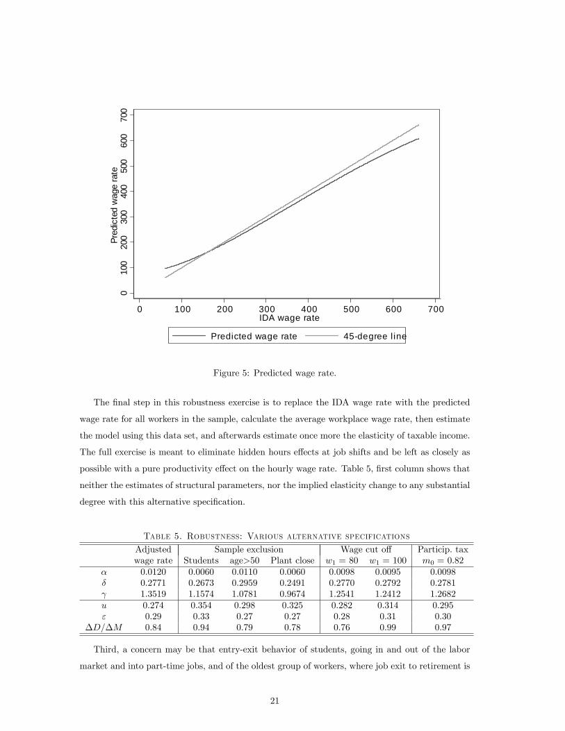
Using this functional form, Figure 5 plots the predicted adjusted wage rate against the IDA wage
and also contains a 45◦-line. The predicted wage rate is lower than than the IDA wage rate in
most of the wage distribution, which is consistent with the existence of overtime work. At the
bottom of the distribution the predicted wage rate is larger than the IDA wage rate, which is
consistent with the WSR data better capturing part-time work.
15Annual labor income is based on tax return data. The Danish Tax Agency obtains third-party informationfrom employers on nearly all labor income in Denmark, and tax evasion on labor income is almost zero (Kleven etal., 2011).16We use the FRACPOLY routine in Stata.
20
010
020
030
040
050
060
070
0Pr
edic
ted
wag
e ra
te
0 100 200 300 400 500 600 700IDA wage rate
Predicted wage rate 45degree l ine
Figure 5: Predicted wage rate.
The final step in this robustness exercise is to replace the IDA wage rate with the predicted
wage rate for all workers in the sample, calculate the average workplace wage rate, then estimate
the model using this data set, and afterwards estimate once more the elasticity of taxable income.
The full exercise is meant to eliminate hidden hours effects at job shifts and be left as closely as
possible with a pure productivity effect on the hourly wage rate. Table 5, first column shows that
neither the estimates of structural parameters, nor the implied elasticity change to any substantial
degree with this alternative specification.
Table 5. Robustness: Various alternative specifications
Adjusted Sample exclusion Wage cut off Particip. taxwage rate Students age>50 Plant close w1 = 80 w1 = 100 m0 = 0.82
Third, a concern may be that entry-exit behavior of students, going in and out of the labor
market and into part-time jobs, and of the oldest group of workers, where job exit to retirement is
21
common, could be important for the results. We have therefore redone the analysis on restricted
samples where students and individuals older than 50 are removed from the sample. Columns 3
and 4 report the results from these two sensitivity tests. The main conclusion is that the elasticity
estimates of 0.27 and 0.33 are rather close to the baseline estimate of 0.30. We have also tried to
remove workers with less than 1 year of work experience. This gives an elasticity equal to 0.35.17
Fourth, we have removed closing plants from the analysis (column 5). This reduces the job
destruction rate, but has little impact on the elasticity estimate, which becomes 0.27. If, in
addition, we remove plants that downsize, identified as a 30 percent reduction or more in the
number of workers as in Jacobson et al. (1993) then we obtain an elasticity of 0.25.
Fifth, we consider two alternative values of the cutoff wage rate w1, DKK 80 and DKK 100.
In each alternative case, w0 is adjusted to preserve w0 = (1−m0)w1, and the P -distribution is
reestimated on the relevant domain. Columns 6 and 7 of Table 5 reveal only small differences in
the parameters and the estimates of the elasticity of taxable income ε lie in the narrow interval
[0.28; 0.31].
Sixth, the participation tax, m0 = 0.59, was in the baseline estimation set at the level of the
lowest marginal tax rates. The results of Kleven and Kreiner (2007) indicate that if the loss of
unemployment/social benefits is included then the participation tax rate on the increase in income
from zero to the lowest possible, full time work income is 82 percent. It is not clear that this is
the right participation tax rate since many of the non-employed will only be entitled to these
benefits for a limited period. However, to explore the possible consequences, we may set m0 equal
to 0.82, keeping all other tax rates unchanged, and again adjust w0 so that w0 = (1−m0)w1
etc. This means that the difference in net income between any two positions i and j is unchanged
from the baseline estimation and hence the estimates of the structural parameters and the rate
of non-employment as well as the elasticity of taxable income are also unchanged. The effi ciency
effect is affected, however, since now a decrease of marginal tax rates will cause a larger behavioral
increase in tax revenue, because T1 − T0 has increased, so there is a larger behavioral tax gain
as non-employment is reduced. Column 8 of Table 5 shows that the estimate of the marginal
excess burden (and therefore the degree of self financing) goes up to 97 percent, so in this case
the considered tax experiment is close to a “Laffer change”.
17We have also tried to run the analysis separately for men and women. This gives an elasticity of 0.35 for menand 0.18 for women. This would from an effi ciency perspective, in isolation, call for higher tax rates on women thanon men. However, with the anonymous tax systems used in practise, it is the overall elasticity of taxable incomethat is relevant for tax policy.
22
6 Concluding remarks
In this paper, we apply a microeconometric, structural analysis to measure the distortionary effects
of taxation on labor mobility and the long run allocation of labor. The analysis points to non-
negligible effects of taxes on labor mobility. We estimate a mobility-based elasticity of taxable
income with respect to the net-of-tax rate in the range 0.15-0.35. This is of the same magnitude
as the estimates found in the empirical public finance literature using difference-in-difference type
methods (Saez et al., 2012) and bunching at kink-points in the tax schedule (Chetty et al., 2011a)
to measure the elasticity of taxable income. The aim of these methods is to capture all relevant
behavioral responses to taxation, thereby obtaining a suffi cient statistic for evaluating the effi ciency
effects of taxation. However, the methods do not provide a clear identification of the effects of
taxation on labor mobility.
We have applied a workhorse, structural model of search and labor mobility for our analysis of
the distortionary effects of taxation on the mobility of labor. The analysis relies on many strong,
simplifying assumptions, as is common when working with structural models. For example, the
empirical identification relies on independence of firm and worker components in wages and an
exogenous distribution of job opportunities, and exploits only cross-sectional variation across
individuals for identification.
The model focuses entirely on involuntary job losses leading to unemployment and voluntary
job-to-job shifts involving upwards wage mobility. In reality labor market mobility is a complex
phenomenon involving changes in geographical location and selling-buying houses, and workers
may voluntarily move to a lower-paid job because of other characteristics of the job or the situation
of the worker. Also, our analysis does not account for higher effort leading to promotions within
firms, which may also lead to discrete jumps in earnings.
The most heroic assumption of the model is probably that all workers are assumed to be
identical, implying that the underlying wage distribution is identical for all individuals. This is
in stark contrast to the labor-leisure framework, underlying the standard identification methods
used to estimate the elasticity of taxable income, where all variation in wages across individuals is
assumed to be fully determined by underlying differences in ability levels, i.e., all workers with the
same ability level will receive the exact same wage. Moreover, in that setting, a little more effort
of the individual will always result in a little more wage income, rather than in a higher chance
of receiving a discrete increase in wage income. Such discrete wage changes, normally observed in
job shifts, are not well identified by the standard methods applied in the large empirical public
finance literature. Thus, although our results rely on a number of strong assumptions, they do
indicate, in our view, that the empirical public finance literature may be overlooking sizable labor
23
mobility effects when measuring the behavioral responses to taxation and the elasticity of taxable
income.
A Derivation of equations (6) and (7)
The derivation proceeds in three steps. In Step 1 we use equation (5) to derive expressions for
g1, ..., gN , which are useful for computing the derivatives ∂gj/∂gi appearing in the first order
conditions (3). In Step 2 we compute ∂u/∂s0 from (4) and ∂gj/∂gi from the expressions for gj
obtained in Step 1. Finally, in Step 3, we insert the expressions for ∂u/∂s0 and ∂gj/∂gi of Step
2 into the first order conditions (2) and (3), and arrive at (6) and (7).
A.1 Step 1
We first show that equation (5) implies
g1 = p1δ
δ + λ (1− P1) s1, and (A-1)
gi =δ
δ + λ (1− P1) s1pi
i−1∏j=1
δ + λ (1− Pj−1) sjδ + λ (1− Pj+1) sj+1
, (A-2)
for i = 2, ..., N . From equation (5), we have
G1 = P1 −λ
δ(1− P1) s1g1.
This may be written as
g1 = p1 −λ
δ(1− P1) s1g1 = p1
δ
δ + λ (1− P1) s1
which is equation (A-1). From equation (5), we get
δGi + λ (1− Pi)i∑
j=1
sjgj = δPi,
and for i ≥ 2, we have
δGi−1 + λ (1− Pi−1)
i−1∑j=1
sjgj = δPi−1.
By subtracting the second from the first of the two expressions above and splitting up summations,
we obtain for i ≥ 2:
δgi + λ
N∑j=i+1
pi
i−1∑j=1
sjgj + sigi
−pi +
N∑j=i+1
pi
i−1∑j=1
sjgj
= δpi,
or
δgi + λ
N∑j=i+1
pi
sigi − pii−1∑j=1
sjgj
= δpi,
24
or
[δ + λ (1− Pi) si] gi = pi
δ + λ
i−1∑j=1
sjgj
or
gi = piδ + λ
∑i−1j=1 sjgj
δ + λ (1− Pi) si. (A-3)
This is a recursive solution for gi, i = 2, ..., N depending on s1, ..., si and g1, ..., gi−1. We derive a
solution for gi+1 only as a function of gi and si and si+1. By leading (A-3), we get
gi+1 = pi+1
δ + λ∑ij=1 sjgj
δ + λ (1− Pi+1) si+1= pi+1
δ + λ∑i−1j=1 sjgj + λsigi
δ + λ (1− Pi+1) si+1.
From (A-3), we have λ∑i−1j=1 sjgj = gi
(δ+λ(1−Pi)si)pi
− δ which inserted in gi+1 gives
(δ + λ (1− Pi+1) si+1) gi+1 = pi+1
(δ + λ (1− Pi) si
pi+ λsi
)gi
which gives
gi+1 =pi+1
pi
δ + λ (1− Pi−1) siδ + λ (1− Pi+1) si+1
gi. (A-4)
By expanding this relationship, we obtain
g2 =p2
p1
δ + λ (1− P0) s1
δ + λ (1− P2) s2g1 = p2
δ + λ (1− P0) s1
δ + λ (1− P2) s2
δ
δ + λ (1− P1) s1,
where we have used (A-1). By expanding further, we get
g3 =p3
p2
δ + λ (1− P1) s2
δ + λ (1− P3) s3g2
= p3δ + λ (1− P1) s2
δ + λ (1− P3) s3
δ + λ (1− P0) s1
δ + λ (1− P2) s2
δ
δ + λ (1− P1) s1
...
gi =δ
δ + λ (1− P1) s1pi
i−1∏j=1
δ + λ (1− Pj−1) sjδ + λ (1− Pj+1) sj+1
,
which is (A-2).
A.2 Step 2
Here, we derive ∂u/∂s0 and ∂gj/∂si. Differentiation of equation (4) gives
∂u
∂s0= − δλ
(λs0 + δ)2 = − λ
λs0 + δu. (A-5)
We show below that differentiation of equations (A-1) and (A-2) give
∂gj∂si
=
0 for j < i
−gi λ(1−Pi)δ+λ(1−Pi)si < 0 for j = iλδpi
(δ+λ(1−Pi−1)si)(δ+λ(1−Pi)si)gj > 0 for j > i
. (A-6)
25
We start by changing indices in (A-2). This gives
gj =δ
δ + λ (1− P1) s1pj
j−1∏h=1
δ + λ (1− Ph−1) shδ + λ (1− Ph+1) sh+1
. (A-7)
We see directly that ∂gj/∂si = 0 for j < i.
By differentiating (A-7) with respect to si for j = i, we get
∂gi∂si
= − δ
δ + λ (1− P1) s1pi
(i−2∏h=1
δ + λ (1− Ph−1) shδ + λ (1− Ph+1) sh+1
)δ + λ (1− Pi−2) si−1
(δ + λ (1− Pi) si)2 λ (1− Pi)
= − δ
δ + λ (1− P1) s1pi
(i−2∏h=1
δ + λ (1− Ph−1) shδ + λ (1− Ph+1) sh+1
)δ + λ (1− Pi−2) si−1
δ + λ (1− Pi) siλ (1− Pi)
δ + λ (1− Pi) si
= − δ
δ + λ (1− P1) s1pi
(i−1∏h=1
δ + λ (1− Ph−1) shδ + λ (1− Ph+1) sh+1
)λ (1− Pi)
δ + λ (1− Pi) si
= −giλ (1− Pi)
δ + λ (1− Pi) si
We now differentiate (A-7) with respect to si for j > i. For i = 1, we have
∂gj∂s1
= −δ λ (1− P1)
(δ + λ (1− P1) s1)2 pj
j−1∏h=1
δ + λ (1− Ph−1) shδ + λ (1− Ph+1) sh+1
+δ
δ + λ (1− P1) s1pj
λ
δ + λs1
j−1∏h=1
δ + λ (1− Ph−1) shδ + λ (1− Ph+1) sh+1
=
[λ
δ + λs1− λ (1− P1)
δ + λ (1− P1) s1
]gj
For i > 1, we get
∂gj∂si
=δ
δ + λ (1− P1) s1pj
(λ (1− Pi−1)
δ + λ (1− Pi−1) si− λ (1− Pi)δ + λ (1− Pi) si
) j−1∏h=1
δ + λ (1− Ph−1) shδ + λ (1− Ph+1) sh+1
=
(λ (1− Pi−1)
δ + λ (1− Pi−1) si− λ (1− Pi)δ + λ (1− Pi) si
)gj
=λδ (Pi − Pi−1)
(δ + λ (1− Pi−1) si) (δ + λ (1− Pi) si)gj
=λδpi
(δ + λ (1− Pi−1) si) (δ + λ (1− Pi) si)gj
This formula also holds for i = 1, which is easily seen by comparing the second equality to the
previous expression for ∂gj/∂s1.
A.3 Step 3
Consider optimal search effort at i = N . In this case, the condition (3) becomes
−c′(sN )gN + [wN − TN − c(sN )]∂gN∂sN
= 0.
26
From equation (A-6), we have ∂gN/∂sN = 0, because PN = 1. Hence, c′(sN ) = 0 giving sN = 0
in (6).
Next, we derive (7). We first consider i ≥ 1. Note that in equation (3) one can let the
summation start in i since from equation (A-6), ∂gj/∂si = 0 for j < i. By isolating c′(si) from
(3), we then obtain
c′(si) =[wi − Ti − c(si)] ∂gi∂si
+∑Nj=i+1 [wj − Tj − c(sj)] ∂gj∂si
gi.
By inserting the derivatives ∂gj/∂si from (A-6), we get