86
Labor Supply Responses to Taxation Stefanie Stantcheva 1 55

Labor Supply Responses to Taxation
Stefanie Stantcheva
1 55

GOALS OF THIS LECTURE
1) Cover empirical studies of labor supply responses to taxation goinghistorically from earlier to more recent papers. Contributes to our highlyimportant “internal paper wikipedia” (IPW).
2) Understand key methodologies such as non-linear budget sets and“bunching at the kinks,” which are useful for a wide range of empirical work.
3) Critically discuss papers’ methodologies and results so as to practice ourresearch skills.
2 55

MOTIVATION
1) Labor supply responses to taxation are of fundamental importance forincome tax policy [efficiency costs and optimal tax formulas]
2) Labor supply responses along many dimensions:
(a) Intensive: hours of work on the job, intensity of work, occupationalchoice [including education]
(b) Extensive: whether to work or not [e.g., retirement and migrationdecisions]
3) Reported earnings for tax purposes can also vary due to (a) taxavoidance [legal tax minimization], (b) tax evasion [illegal under-reporting]
4) Different responses in short-run and long-run: long-run response mostimportant for policy but hardest to estimate
3 55

BASIC CROSS SECTION ESTIMATION
Data on hours or work, wage rates, non-labor income started becomingavailable in the 1960s when first micro surveys and computers appeared:
Simple OLS regression:
li = α + βwi + γyi + Xiδ + εi
wi is the net-of-tax wage rate
yi measures non-labor income [including spousal earnings for couples]
Xi are demographic controls [age, experience, education, etc.]
β measures uncompensated wage effects, and γ income effects [can beconverted to εu , η]
4 55

BASIC CROSS SECTION RESULTS
1. Male workers [primary earners when married] (Pencavel, 1986 survey):
a) Small effects εu = 0, η = −0.1, εc = 0.1 with some variation acrossestimates (sometimes εc < 0).
2. Female workers [secondary earners when married] (Killingsworth andHeckman, 1986):
Much larger elasticities on average, with larger variations across studies.Elasticities go from zero to over one. Average around 0.5. Significantincome effects as well
Female labor supply elasticities have declined overtime as women becomemore attached to labor market (Blau-Kahn JOLE’07)
5 55
KEY ISSUE: w correlated with tastes for work
li = α + βwi + γyi + εiIdentification is based on cross-sectional variation in wi : comparing hoursof work of highly skilled individuals (high wi ) to hours of work of lowskilled individuals (low wi )
If highly skilled workers have more taste for work (independent of the wageeffect), then εi is positively correlated with wi leading to an upward bias inOLS
Plausible scenario: hard workers acquire better education and hence havehigher wages
Controlling for Xi can help but can never be sure that we have controlledfor all the factors correlated with wi and tastes for work: Omitted variablebias
⇒ Tax changes provide more compelling identification6 55

TAX ISSUE: NON-LINEAR BUDGET SETS
Actual tax system is not linear but piece-wise linear with varying marginaltax rate τ due to (a) means-tested transfer programs, (b) progressiveindividual income tax
Same theory applies when considering the linearized tax systemc = wl + y with w = wp(1−T ′) and y defined as virtual income (interceptof budget with x-axis when setting l = 0)
Main complications:
(a) w [and y ] become endogenous to choice of l
(b) FOC may not hold if individual bunches at a kink
(c) FOC may not characterize the optimum choice
7 55

Non-Linear Budget Set Estimation: Virtual Incomes
Raj Chetty () Labor Supply Harvard, Fall 2009 24 / 156
TAX ISSUE: NON-LINEAR BUDGET SETS
Non-linear budget set creates two econometric problems:
1) Model mis-specification: OLS regression no longer recovers structuralelasticity parameter of interest
2) Econometric bias: τi = T ′(wi li ) and yi depends on income wi li andhence on li
Tastes for work are positively correlated with τi (due to progressive taxsystem) → downward bias in OLS regression of hours worked on net-of-taxrates
8 55

OLD NON-LINEAR BUDGET SET METHOD
Issue addressed by non linear budget set studies pioneered by Hausman inlate 1970s (Hausman, 1985 PE handbook chapter)
Method uses a structural model of labor supply to derive and estimatelabor supply function fully consistent with theory
Key point: the method still uses the standard cross-sectional variation inpre-tax wages wp for identification. Taxes are seen as a problem to dealwith rather than an opportunity for identification.
New literature identifying labor supply elasticities using tax changes has atotally different perspective: taxes are seen as an opportunity to identifylabor supply
9 55

Negative Income Tax (NIT) Experiments
1) Best way to resolve identification problems: exogenously changetaxes/transfers with a randomized experiment
2) NIT experiment conducted in 1960s/70s in Denver, Seattle, and othercities
3) First major social experiment in U.S. designed to test proposed transferpolicy reform
4) Provided lump-sum welfare grants G combined with a steep phaseoutrate τ (50%-80%) [based on family earnings]
5) Analysis by Rees (1974), Munnell (1986) book, Ashenfelter and PlantJOLE’90, and others
6) Several groups, with randomization within each; approx. N = 75households in each group
10 55

Raj Chetty () Labor Supply Harvard, Fall 2009 87 / 156
Source: Ashenfelter and Plant (1990), p. 403

NIT Experiments: Findings
See Ashenfelter and Plant JHR’ 90 for non-parametric evidence. Moreparametric evidence in earlier work. Key results:
1) Significant labor supply response but small overall
2) Implied earnings elasticity for males around 0.1
3) Implied earnings elasticity for women around 0.5
4) Academic literature not careful to decompose response along intensiveand extensive margin
5) Response of women is concentrated along the extensive margin (can onlybe seen in official govt. report)
6) Earnings of treated women who were working before the experiment didnot change much
11 55
From true experiment to “natural experiments”
True experiments are costly to implement and hence rare
However, real economic world (nature) provides variation that can beexploited to estimate behavioral responses ⇒ “Natural Experiments”
Natural experiments sometimes come very close to true experiments:Imbens, Rubin, Sacerdote AER ’01 did a survey of lottery winners andnon-winners matched to Social Security administrative data to estimateincome effects
Lottery generates random assignment conditional on playing
Find significant but relatively small income effects: η = w∂l/∂y between-0.05 and -0.10
12 55

784 THE AMERICAN ECONOMIC REVIEW SEPTEMBER 2001
co 0.8-
0.6 -
0~ *'0.4 ..
0
-6 -4 -2 0 2 4 6 Year Relative to Winning
FIGURE 2. PROPORTION WITH POSITIVE EARNINGS FOR NONWINNERS, WINNERS, AND BIG WINNERS
Note: Solid line = nonwinners; dashed line = winners; dotted line = big winners.
type accounts, including IRA's, 401(k) plans, and other retirement-related savings. The sec- ond consists of stocks, bonds, and mutual funds and general savings.13 We construct an addi- tional variable "total financial wealth," adding up the two savings categories.14 Wealth in the various savings accounts is somewhat higher than net wealth in housing, $133,000 versus $122,000. The distributions of these financial wealth variables are very skewed with, for ex- ample, wealth in mutual funds for the 414 re- spondents ranging from zero to $1.75 million, with a mean of $53,000, a median of $10,000, and 35 percent zeros.
The critical assumption underlying our anal- ysis is that the magnitude of the lottery prize is random. Given this assumption the background characteristics and pre-lottery earnings should not differ significantly between nonwinners and winners. However, the t-statistics in Table 1 show that nonwinners are significantly more educated than winners, and they are also older.
This likely reflects the differences between sea- son ticket holders and single ticket buyers as the differences between all winners and the big winners tend to be smaller.15 To investigate further whether the assumption of random as- signment of lottery prizes is more plausible within the more narrowly defined subsamples, we regressed the lottery prize on a set of 21 pre-lottery variables (years of education, age, number of tickets bought, year of winning, earn- ings in six years prior to winning, dummies for sex, college, age over 55, age over 65, for working at the time of winning, and dummies for positive earnings in six years prior to win- ning). Testing for the joint significance of all 21 covariates in the full sample of 496 observations led to a chi-squared statistic of 99.9 (dof 21), highly significant (p < 0.001). In the sample of 237 winners, the chi-squared statistic was 64.5, again highly significant (p < 0.001). In the sample of 193 small winners, the chi-squared statistic was 28.6, not significant at the 10- percent level. This provides some support for assumption of random assignment of the lottery prizes, at least within the subsample of small winners. 13 See the Appendix in Imbens et al. (1999) for the
questionnaire with the exact formulation of the questions. 14 To reduce the effect of item nonresponse for this last
variable, total financial wealth, we added zeros to all miss- ing savings categories for those people who reported posi- tive savings for at least one of the categories. That is, if someone reports positive savings in the category "retire- ment accounts," but did not answer the question for mutual funds, we impute a zero for mutual funds in the construction of total financial wealth. For the 462 observations on total financial wealth, zeros were imputed for 27 individuals for retirement savings and for 30 individuals for mutual funds and general savings. As a result, the average of the two savings categories does not add up to the average of total savings, and the number of observations for the total savings variable is larger than that for each of the two savings categories.
15 Although the differences between small and big win- ners are smaller than those between winners and losers, some of them are still significant. The most likely cause is the differential nonresponse by lottery prize. Because we do know for all individuals, respondents or nonrespondents, the magnitude of the prize, we can directly investigate the correlation between response and prize. Such a non-zero correlation is a necessary condition for nonresponse to lead to bias. The t-statistic for the slope coefficient in a logistic regression of response on the logarithm of the yearly prize is -3.5 (the response rate goes down with the prize), lending credence to this argument.
Source: Imbens et al (2001), p. 784

VOL. 91 NO. 4 IMBENS ET AL.: EFFECTS OF UNEARNED INCOME 783
m 0 , " .........
10-
O
-6 -4 -2 0 2 4 6 Year Relative to Winning
FIGURE 1. AVERAGE EARNINGS FOR NONWINNERS, WINNERS, AND BIG WINNERS
Note: Solid line = nonwinners; dashed line = winners; dotted line = big winners.
On average the individuals in our basic sample won yearly prizes of $26,000 (averaged over the $55,000 for winners and zero for nonwinners). Typically they won 10 years prior to completing our survey in 1996, implying they are on average halfway through their 20 years of lottery payments when they responded in 1996. We asked all indi- viduals how many tickets they bought in a typical week in the year they won the lottery.!1 As ex- pected, the number of tickets bought is consider- ably higher for winners than for nonwinners. On average, the individuals in our basic sample are 50 years old at the time of winning, which, for the average person was in 1986; 35 percent of the sample was over 55 and 15 percent was over 65 years old at the time of winning; 63 percent of the sample was male. The average number of years of schooling, calculated as years of high school plus years of college plus 8, is equal to 13.7; 64 percent claimed at least one year of college.
We observe, for each individual in the basic sample, Social Security earnings for six years pre- ceding the time of winning the lottery, for the year they won (year zero), and for six years following winning. Average earnings, in terms of 1986 dol- lars, rise over the pre-winning period from $13,930 to $16,330, and then decline back to $13,290 over the post-winning period. For those with positive Social Security earnings, average earnings rise over the entire 13-year period from $20,180 to $24,300. Participation rates, as mea- sured by positive Social Security earnings, grad-
ually decline over the 13 years, starting at around 70 percent before going down to 56 percent. Fig- ures 1 and 2 present graphs for average earnings and the proportion of individuals with positive earnings for the three groups, nonwinners, win- ners, and big winners. One can see a modest decline in earnings and proportion of individuals with positive earnings for the full winner sample compared to the nonwinners after winning the lottery, and a sharp and much larger decline for big winners at the time of winning. A simple difference-in-differences type estimate of the mar- ginal propensity to earn out of unearned income (mpe) can be based on the ratio of the difference in the average change in earnings before and after winning the lottery for two groups and the differ- ence in the average prize for the same two groups. For the winners, the difference in average earnings over the six post-lottery years and the six pre- lottery years is -$1,877 and for the nonwinners the average change is $448. Given a difference in average prize of $55,000 for the winner/nonwin- ners comparison, the estimated mpe is (- 1,877 - 448)/(55,000 - 0) = -0.042 (SE 0.016). For the big-winners/small-winners comparison, this esti- mate is -0.059 (SE 0.018). In Section IV we report estimates for this quantity using more so- phisticated analyses.
On average the value of all cars was $18,200. For housing the average value was $166,300, with an average mortgage of $44,200.12 We aggregated the responses to financial wealth into two categories. The first concerns retirement
" Because there were some extremely large numbers (up to 200 tickets per week), we transformed this valiable somewhat arbitrarily by taking the minimum of the number reported and ten. The results were not sensitive to this transformation.
12 Note that this is averaged over the entire sample, with zeros included for the 7 percent of respondents who re- ported not owning their homes.
Source: Imbens et al. (2001), p. 783
Difference-in-Difference (DD) methodology
Two groups: Treatment group (T) which faces a change [lottery winners]and control group (C) which does not [non winners]
Compare the evolution of T group (before and after change) to the evolutionof the C group (before and after change)
DD identifies the treatment effect if the parallel trend assumption holds:
Absent the change, T and C would have evolved in parallel
DD most convincing when groups are very similar to start with
Should always test DD using data from more periods and plot the two timeseries to check parallel trend assumption
13 55

Married Women Elasticities: Blau and Kahn ’07
1) Identify elasticities from 1980-2000 using grouping instrument
a) Define cells (year×age×education) and compute mean wages
b) Instrument for actual wage with mean wage in cell
2) Identify purely from group-level variation, which is less contaminated byindividual endogenous choice
3) Results: (a) total hours elasticity for married women (including intensive+ extensive margin) shrank from 0.4 in 1980 to 0.2 in early 2000s, (b) effectof husband earnings ↓ overtime
4) Interpretation: elasticities shrink as women become more attached to thelabor force
14 55

Summary of Static Labor Supply Literature (SKIP)
1) Small elasticities for prime-age males
Probably institutional restrictions, need for at least one income, etc.prevent a short-run response
2) Larger responses for workers who are less attached to labor force:Married women, low income earners, retirees
3) Responses driven primarily by extensive margin
a) Extensive margin (participation) elasticity around 0.2-0.5
b) Intensive margin (hours) elasticity smaller
15 55

Responses to Low-Income Transfer Programs
1) Particular interest in treatment of low incomes in a progressive taxsystem: are they responsive to incentives?
2) Complicated set of transfer programs in US
a) In-kind: food stamps, Medicaid, public housing, job training, educationsubsidies
b) Cash: TANF, EITC, SSI
3) See Gruber undergrad textbook for details on institutions
16 55

1996 US Welfare Reform
1) Reform modified AFDC cash welfare program to provide more incentivesto work (renamed TANF)
a) Requiring recipients to go to job training or work
b) Limiting the duration for which families able to receive welfare
c) Reducing phase-out rate of benefits
2) Fed govt provided incentives for states to experiment with reforms in1992-1995 (state waivers). Some did randomized experiments.
4) EITC also expanded during this period: general shift from welfare to“workfare”
Did welfare reform and EITC increase labor supply?
17 55
TANF: Size and Characteristics of the Cash Assistance Caseload
Congressional Research Service 4
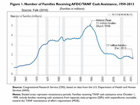
Figure 1. Number of Families Receiving AFDC/TANF Cash Assistance, 1959-2013
(Families in millions)
Source: Congressional Research Service (CRS), based on data from the U.S. Department of Health and Human
Services (HHS).
Notes: Shaded areas represent recessionary periods. Families receiving TANF cash assistance since October 1,
1999, include families receiving cash assistance from separate state programs (SSPs) with expenditures countable
toward the TANF maintenance of effort requirement (MOE).
Trends in Caseload Characteristics:
FY1988 to FY2013 The increases in the cash assistance caseload from 1989 to 1994, and its decline thereafter, were
also associated with changes in the character of the caseload. Table 1 provides an overview of the
characteristics of the family cash assistance caseload for selected years: FY1988, FY1994,
FY2001, FY2006, and FY2013.10
The most dramatic change in caseload characteristics is the
growth in the share of families with no adult recipients. In FY2013, 38.1% of TANF assistance
families had no adult recipient; in contrast, in FY1988 only 9.8% of all cash assistance families
had no adult recipient. These are families with ineligible adults (sometimes parents, sometimes
other relatives) but whose children are eligible and receive benefits.
10 Caseload characteristic data in this report are based on information states are required to report to HHS under their
AFDC and TANF programs. Efforts were made to make the data comparable across the years, but some changes in
reporting as well as other program requirements affect the comparability of the data. The major difference is that for
FY2013, TANF families “with an adult recipient” include those families where the adult has been time-limited or
sanctioned but the family continues to receive a reduced benefit. These are technically “child-only” cases, because the
adult does not receive a benefit. However, since FY2007 such families have been subject to TANF work participation
standards and thus the policy affecting them is more comparable to that of a family with an adult recipient than a
“child-only” family. For years before FY2007, these families were not subject to work participation standards and are
classified together with other “child-only” families. The data to identify them separately prior to FY2007 are not
comparable to data for FY2007 and subsequent years.
Source: Falk (2016)

The landscape providing assistance to poor families with children has changed substantially
175
200Contractions
AFDC/TANF Cash Benefits Per CapitaFederal welfare reform
125
150
ditures
Food Stamp Expenditures Per Capita
EITC Expenditures Per Capita
100
125
Real Expend
50
75
Per C
apita
25
4
0
1980 1985 1990 1995 2000 2005

Earned Income Tax Credit (EITC) program
See Kleven (2018) provides comprehensive ex-post re-analysis usingwomen aged 20-50 and CPS data
1) EITC started small in the 1970s but was expanded in 1986-88, 1994-96,2008-09: today, largest means-tested cash transfer program [$70bn in2016, 30m families recipients]
2) Eligibility: families with kids and low earnings.
3) Refundable Tax credit: administered as annual tax refund received inFeb-April, year t + 1 (for earnings in year t)
4) EITC has flat pyramid structure with phase-in (negative MTR), plateau,(0 MTR), and phase-out (positive MTR)
5) States have added EITC components to their income taxes [in general apercentage of the Fed EITC, great source of natural experiments,understudied bc CPS too small]
18 55

EITC Schedule in 2017
0 children
1 child
2 children
3+ children
020
0040
0060
00An
nual
Cre
dit (
USD
)
0 10000 20000 30000 40000 50000 60000Earnings (USD)
7 / 167

EITC Maximum Credit Over Time
0 children
1 child
2 children
3+ children
Tax ReductionAct of 1975 TRA86 OBRA90 OBRA93 ARRA
02,
000
4,00
06,
000
Max
imum
Ann
ual C
redi
t (20
17 U
SD)
68 70 72 74 76 78 80 82 84 86 88 90 92 94 96 98 00 02 04 06 08 10 12 14 16 18Year
8 / 167
Source: Kleven (2018)

Labor Force Participation of Single WomenWith and Without Children
2.6
4.6
Une
mpl
oym
ent R
ate
5060
7080
9010
0La
bor F
orce
Par
ticip
atio
n (%
)
68 70 72 74 76 78 80 82 84 86 88 90 92 94 96 98 00 02 04 06 08 10 12 14 16 18Year
With Children Without Children
Annual Employment Low Education13 / 167
Source: Kleven (2018)

Labor Force Participation of Single WomenWith and Without Children
50 years of relative stability,apart from these 5 years
2.6
4.6
Une
mpl
oym
ent R
ate
5060
7080
9010
0La
bor F
orce
Par
ticip
atio
n (%
)
68 70 72 74 76 78 80 82 84 86 88 90 92 94 96 98 00 02 04 06 08 10 12 14 16 18Year
With Children Without Children
Annual Employment Low Education14 / 167
Source: Kleven (2018)

Labor Force Participation of Single WomenWith and Without Children
14.5pp
14pp
50 years of relative stability,apart from these 5 years
2.6
4.6
Une
mpl
oym
ent R
ate
5060
7080
9010
0La
bor F
orce
Par
ticip
atio
n (%
)
68 70 72 74 76 78 80 82 84 86 88 90 92 94 96 98 00 02 04 06 08 10 12 14 16 18Year
With Children Without Children
Annual Employment Low Education15 / 167
Source: Kleven (2018)

Labor Force Participation of Single WomenWith and Without Children
Tax ReductionAct of 1975 TRA86 OBRA90 OBRA93 ARRA
2.6
4.6
Unem
ploy
men
t Rat
e
5060
7080
9010
0La
bor F
orce
Par
ticip
atio
n (%
)
68 70 72 74 76 78 80 82 84 86 88 90 92 94 96 98 00 02 04 06 08 10 12 14 16 18Year
With Children Without Children
Annual Employment Low Education16 / 167
Source: Kleven (2018)

Labor Force Participation of Single WomenWith and Without Children
Tax ReductionAct of 1975 TRA86 OBRA90 OBRA93 ARRAPRWORA
2.6
4.6
Unem
ploy
men
t Rat
e
5060
7080
9010
0La
bor F
orce
Par
ticip
atio
n (%
)
68 70 72 74 76 78 80 82 84 86 88 90 92 94 96 98 00 02 04 06 08 10 12 14 16 18Year
With Children Without Children
Annual Employment Low Education17 / 167
Source: Kleven (2018)

Labor Force Participation of Single WomenWith and Without Children
Tax ReductionAct of 1975 TRA86 OBRA90 OBRA93 ARRAPRWORA
State WelfareWaivers
2.6
4.6
Unem
ploy
men
t Rat
e
5060
7080
9010
0La
bor F
orce
Par
ticip
atio
n (%
)
68 70 72 74 76 78 80 82 84 86 88 90 92 94 96 98 00 02 04 06 08 10 12 14 16 18Year
With Children Without Children
Annual Employment Low Education18 / 167
Source: Kleven (2018)

Labor Force Participation of Single WomenWith and Without Children
Tax ReductionAct of 1975 TRA86 OBRA90 OBRA93 ARRAPRWORA
State WelfareWaivers
46
810
Unem
ploy
men
t Rat
e
5060
7080
9010
0La
bor F
orce
Par
ticip
atio
n (%
)
68 70 72 74 76 78 80 82 84 86 88 90 92 94 96 98 00 02 04 06 08 10 12 14 16 18Year
With Children Without Children Unemployment
Annual Employment Low Education19 / 167
Source: Kleven (2018)
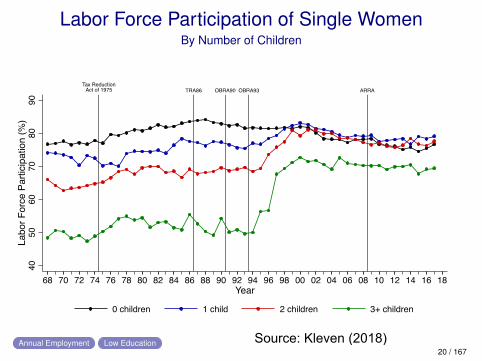
Labor Force Participation of Single WomenBy Number of Children
Tax ReductionAct of 1975 TRA86 OBRA90 OBRA93 ARRA
4050
6070
8090
Labo
r For
ce P
artic
ipat
ion
(%)
-1 -.5 0 .5 1
68 70 72 74 76 78 80 82 84 86 88 90 92 94 96 98 00 02 04 06 08 10 12 14 16 18Year
0 children 1 child 2 children 3+ children
Annual Employment Low Education20 / 167
Source: Kleven (2018)

Labor Force Participation of Single WomenBy Number of Children
Tax ReductionAct of 1975 TRA86 OBRA90 OBRA93 ARRA
Much larger increaseby those with 3+ kids40
5060
7080
90La
bor F
orce
Par
ticip
atio
n (%
)
-1 -.5 0 .5 1
68 70 72 74 76 78 80 82 84 86 88 90 92 94 96 98 00 02 04 06 08 10 12 14 16 18Year
0 children 1 child 2 children 3+ children
Annual Employment Low Education21 / 167
Source: Kleven (2018)

Labor Force Participation of Single WomenBy Number of Children
Tax ReductionAct of 1975 TRA86 OBRA90 OBRA93 ARRA
But no increase hereby those with 3+ kids
4050
6070
8090
Labo
r For
ce P
artic
ipat
ion
(%)
-1 -.5 0 .5 1
68 70 72 74 76 78 80 82 84 86 88 90 92 94 96 98 00 02 04 06 08 10 12 14 16 18Year
0 children 1 child 2 children 3+ children
Annual Employment Low Education22 / 167
Source: Kleven (2018)

FIGURE 6: DID EVENT STUDIES OF ALL FEDERAL EITC REFORMS
A: 1975 Reform, With vs Without Children B: 1986 and 1990 Reforms, With vs Without Children
TRA1975
-10
-50
510
1520
Impa
ct o
n Em
ploy
men
t (pp
)
70 71 72 73 74 75 76 77 78 79 80 81Year
TRA1986 OBRA90
-10
-50
510
1520
Impa
ct o
n Em
ploy
men
t (pp
)
82 83 84 85 86 87 88 89 90 91 92 93Year
C: 1993 Reform, With vs Without Children D: 2009 Reform, 3+ vs Without Children
OBRA1993 PRWORA
-10
-50
510
1520
Impa
ct o
n Em
ploy
men
t (pp
)
89 90 91 92 93 94 95 96 97 98 99 00Year
ARRA
-10
-50
510
1520
Impa
ct o
n Em
ploy
men
t (pp
)
04 05 06 07 08 09 10 11 12 13 14 15Year
Notes: This figure shows DiD event studies for the five federal EITC reforms. The graphs plot estimates of γt based on specification (1) without demographic controls.Panels A-C are based on comparing single women with and without children, while Panel D is based on comparing single women with 3+ children to those withoutchildren. In each panel, the difference in the pre-reform year is normalized to zero. The dependent variable is weekly employment. The sample includes singlewomen aged 20-50. Panels A-B use the March CPS files alone, while Panels C-D use the March and monthly files combined. The 95% confidence intervals are basedon robust standard errors clustered at the individual level.
54

FIGURE 7: A FANNING-OUT BY NUMBER OF CHILDREN
A: Raw DataOBRA93 PRWORA
1 Kid
2 Kids
3 Kids
4+ Kids
-10
010
2030
Impa
ct o
n Em
ploy
men
t (pp
)
89 90 91 92 93 94 95 96 97 98 99 00 01 02 03Year
B: Controlling for DemographicsOBRA93 PRWORA
1 Kid
2 Kids
3 Kids
4+ Kids
-10
010
2030
Impa
ct o
n Em
ploy
men
t (pp
)
89 90 91 92 93 94 95 96 97 98 99 00 01 02 03Year
Notes: This figure shows DiD event studies for the 1993 reform by number of EITC-eligible children (1, 2, 3, 4+). Thegraphs plot DiD coefficients γt based on an extension of specification (1) that includes dummies for each family size.Hence, each series shows the difference between single mothers with a given number of children and single womenwithout children, normalized to zero in 1993. Panel A shows raw estimates, while panel B controls for demographiccomposition: dummies for the age of the woman (six categories), dummies for the age of the youngest child (sevencategories), and dummies for education (three categories). The dependent variable is weekly employment. The sampleincludes single women aged 20-50 using the March and monthly CPS files combined.
55

Welfare Reform and EITC Expansion: Labor supply
Incredible increase in labor force participation of single mothers during the1990s when welfare reform and EITC expansion happened
Kleven (2018): Unlikely that only the EITC can explain it because otherEITC changes haven’t generated such large effects. Maybe a uniquecombination of EITC reform, welfare reform, economic upturn, and changingsocial norms lead to this shift
Or informational effects.
RCTs have consistently shown an effect of EITC and in-work tax credits.
Note: Even if EITC had no labor supply responses, this does not mean it’snot a valuable transfer program.
21 55

Theoretical Behavioral Responses to the EITC
Extensive margin: positive effect on Labor Force Participation as EITCmakes work more attractive
Intensive margin: earnings conditional on working, mixed effects
1) Phase in: (a) Substitution effect: work more due to wage subsidy, (b)Income effect: work less ⇒ Net effect: ambiguous; probably work more
2) Plateau: Pure income effect (no change in net wage) ⇒ Net effect: workless
3) Phase out: (a) Substitution effect: work less, (b) Income effect: also workless ⇒ Net effect: work less
Should expect bunching at the EITC kink points
22 55

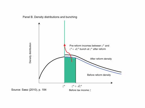
Bunching at Kinks (Saez AEJ-EP’10)
Key prediction of standard labor supply model: individuals should bunch at(convex) kink points of the budget set
1) The only non-parametric source of identification for intensive elasticityin a single cross-section of earnings is amount of bunching at kinkscreating by tax/transfer system
2) Saez ’10 develops method of using bunching at kinks to estimate thecompensated income elasticity
Formula for elasticity: εc = dz/z∗dt/(1−t) = excess mass at kink / change in
NTR
⇒ Amount of bunching proportional to compensated elasticity
Blomquist-Newey 2017: Bunching method requires making assumptions oncounterfactual density (but testable using tax changes see Londono-Avila’18 below)
23 55

184 AmErICAN ECoNomIC JoUrNAL: ECoNomIC PoLICy AUgUST 2010
elasticity e would no longer be a pure compensated elasticity, but a mix of the com-pensated elasticity and the uncompensated elasticity. Four points should be noted.
First, the larger the behavioral elasticity, the more bunching we should expect. Unsurprisingly, if there are no behavioral responses to marginal tax rates, there
Panel A. Indifference curves and bunching
Before tax income z
Slope 1− t
z* z*+ dz*
Slope 1− t−dt
Individual L chooses z* before and after reform
Individual H chooses z*+ dz* before and z* after reform
dz*/z* = e dt/(1− t) with e compensated elasticity
Individual H indifference curves
Individual L indifference curve
Panel B. Density distributions and bunching
Den
sity
dis
trib
utio
n
Before reform density
After reform density
Pre-reform incomes between z* andz*+ dz* bunch at z* after reform
Before tax income zz* z*+ dz*
Afte
r-ta
x in
com
e c
= z
−T(z
)
Figure 1. Bunching Theory
Notes: Panel A displays the effect on earnings choices of introducing a (small) kink in the budget set by increasing the tax rate t by dt above income level z*. Individual L who chooses z* before the reform stays at z* after the reform. Individual h chooses z* after the reform and was choosing z* + dz* before the reform. Panel B depicts the effects of introducing the kink on the earnings density distribution. The pre-reform density is smooth around z*. After the reform, all individuals with income between z* and z* + dz* before the reform, bunch at z*, creating a spike in the density dis-tribution. The density above z* + dz* shifts to z* (so that the resulting density and is no longer smooth at z*).
Source: Saez (2010), p. 184

188 AmErICAN ECoNomIC JoUrNAL: ECoNomIC PoLICy AUgUST 2010
implemented with larger sample size.10 As we shall see, in some cases, the elasticity estimate is sensitive to the choice of δ. The simplest method to select δ is graphical to ensure that the full excess bunching is included in the band (z* − δ, z* + δ) as in Figure 2.
Empirically, h(z*)− can be estimated as the fraction of individuals in the lower surrounding band (z* − 2δ, z* − δ) divided by δ. Similarly, h(z*)+ can be esti-mated as the fraction of individuals in the upper surrounding band (z* + δ, z* + 2δ) divided by δ. We estimate the number of individuals in each of the three bands, which we denote by ˆ
h *−, ˆ
h *, ˆ
h *+, by regressing (simultaneously) a dummy variable for belonging to each band on a constant in the sample of individuals belonging to any of those three bands. We can then compute ̂
h (z*)+ = ˆ
h *+/δ, ̂
h (z*)− = ˆ
h *−/δ and
ˆ
B = ˆ
h * − ( ˆ h *+ + ˆ
h *−) to estimate ̂ e .
10 Chetty et al. (2009) use much larger samples in Denmark and take into account such curvature by estimating the density nonparametrically outside the bunching segment [z* − δ, z* + δ ].
Den
sity
dis
trib
utio
n
Before tax income z
h(z)h(z*)−
h(z*)+ B = H*− (H*− + H*+) = excess bunching
Before reform: linear tax rate t0,density h0 (z)
After reform: tax rate t0 below z*Tax rate t1 above z* ( t1 > t0 ), density h(z)
H*− H*+ h0 (z)
h(z)z*
−2δ z*
z*+
2δ
z*+
δ
z*−
δ
Figure 2. Estimating Excess Bunching Using Empirical Densities
Notes: The figure illustrates the excess bunching estimation method using empirical densities. We assume that, under a constant linear tax with rate t0, the density of income h0(z) is smooth. A higher tax rate t1 is introduced above z*, creating a convex kink at z*. The reform will induce tax filers to cluster at z*, creating a spike in the post-reform density distribution h(z). As illustrated on the figure, bunching might not be perfectly concentrated at z* because of inability of tax filers to control or forecast their incomes perfectly or imperfect information about the exact kink location. For estimation purposes, we define three bands of income around the kink point z* using the bandwidth parameter δ. The lower band is the segment (z*−2δ, z*−δ ), it has average density h(z*)− and hence includes h*−= δ h(z*)− tax filers (dashed left area). The upper band is the segment (z* + δ, z* + 2δ ), it has average density h(z*)+ and hence includes h*+ = δ h(z*)+ tax filers (dashed right area). The middle band is the segment (z* −δ,z* + δ ) and includes h* tax filers. Excess bunching is defined as B = h* − (h*− − h*+) and is the upper dashed area on the figure. If clustering of tax filers around z* is tight, excess bunching will be estimated without bias with a small δ. If clustering is not tight around z*, a small δ will underestimate the amount of excess bunching (as the lower and upper bands will include tax filers clustering around z*). However, a large δ will lead to overestimate (under-estimate) excess bunching if the before reform density h0(z) is convex (concave) around z*.

Bunching at Kinks (Saez AEJ-EP’10)
1) Uses individual tax return micro data (IRS public use files) from 1960 to2004
2) Advantage of dataset over survey data: very little measurement error
3) Finds bunching around:
a) First kink point of the Earned Income Tax Credit (EITC), especially forself-employed
b) At threshold of the first tax bracket where tax liability starts, especiallyin the 1960s when this point was very stable
4) However, no bunching observed around all other kink points
24 55
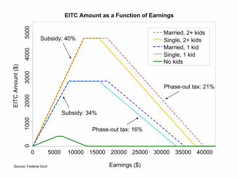
EITC Amount as a Function of Earnings
Earnings ($)
0 5000 10000 15000 20000 25000 30000 35000 40000
Subsidy: 34%
Subsidy: 40%
Phase-out tax: 16%
Phase-out tax: 21%
Single, 2+ kidsMarried, 2+ kids
Single, 1 kidMarried, 1 kid
No kids
EIT
C A
mou
nt ($
)
010
0020
0030
0040
0050
00
Source: Federal Govt

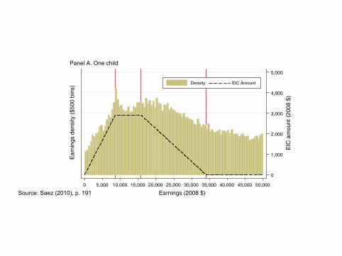
VoL. 2 No. 3 191SAEz: do TAxPAyErS BUNCh AT kINk PoINTS?
indexes earnings to 2008 using the IRS inflation parameters, so that the EITC kinks are perfectly aligned for all years.
Two elements are worth noting in Figure 3. First, there is a clear clustering of tax filers around the first kink point of the EITC. In both panels, the density is maximum exactly at the first kink point. The fact that the location of the first kink point differs between EITC recipients with one child, versus those with two or more children, con-stitutes strong evidence that the clustering is driven by behavioral responses to the EITC as predicted by the standard model. Second, however, we cannot discern any
5,000
4,000
3,000
2,000
1,000
0
EIC
am
ount
(20
08 $
)
Ear
ning
s de
nsity
($5
00 b
ins)
0 5,000 10,000 15,000 20,000 25,000 30,000 35,000 40,000 45,000 50,000
Earnings (2008 $)
Density EIC Amount
Panel A. One child
Ear
ning
s de
nsity
($5
00 b
ins)
0 5,000 10,000 15,000 20,000 25,000 30,000 35,000 40,000 45,000 50,000
Earnings (2008 $)
B. Two children or more
Density EIC Amount
5,000
4,000
3,000
2,000
1,000
0
EIC
am
ount
($)
Figure 3. Earnings Density Distributions and the EITC
Notes: The figure displays the histogram of earnings (by $500 bins) for tax filers with one dependent child (panel A) and tax filers with two or more dependent children (panel B). The histogram includes all years 1995–2004 and inflates earnings to 2008 dollars using the IRS inflation parameters (so that the EITC kinks are aligned for all years). Earnings are defined as wages and salaries plus self-employment income (net of one-half of the self-employed pay-roll tax). The EITC schedule is depicted in dashed line and the three kinks are depicted with vertical lines. Panel A is based on 57,692 observations (representing 116 million tax returns), and panel B on 67,038 observations (repre-senting 115 million returns).
Source: Saez (2010), p. 191

192 AmErICAN ECoNomIC JoUrNAL: ECoNomIC PoLICy AUgUST 2010
systematic clustering around the second kink point of the EITC. Similarly, we cannot discern any gap in the distribution of earnings around the concave kink point where the EITC is completely phased-out. This differential response to the first kink point, versus the other kink points, is surprising in light of the standard model predicting that any convex (concave) kink should produce bunching (gap) in the distribution of earnings.
In Figure 4, we break down the sample of earners into those with nonzero self-employment income versus those zero self-employment income (and hence whose
5,000
4,000
3,000
2,000
1,000
0
5,000
4,000
3,000
2,000
1,000
0
EIC
am
ount
($)
EIC
am
ount
($)
Ear
ning
s de
nsity
0 5,000 10,000 15,000 20,000 25,000 30,000 35,000 40,000 45,000 50,000
Earnings (2008 $)
Wage earners
Self-employed
EIC amount
Panel A. One child
Ear
ning
s de
nsity
0 5,000 10,000 15,000 20,000 25,000 30,000 35,000 40,000 45,000 50,000
Earnings (2008 $)
Panel B. Two or more children
Wage earners
Self-employed
EIC amount
Figure 4. Earnings Density and the EITC: Wage Earners versus Self-Employed
Notes: The figure displays the kernel density of earnings for wage earners (those with no self-employment earnings) and for the self-employed (those with nonzero self employment earnings). Panel A reports the density for tax fil-ers with one dependent child and panel B for tax filers with two or more dependent children. The charts include all years 1995–2004. The bandwidth is $400 in all kernel density estimations. The fraction self-employed in 16.1 per-cent and 20.5 percent in the population depicted on panels A and B (in the data sample, the unweighted fraction self-employed is 32 percent and 40 percent). We display in dotted vertical lines around the first kink point the three bands used for the elasticity estimation with δ = $1,500.
Source: Saez (2010), p. 192

192 AmErICAN ECoNomIC JoUrNAL: ECoNomIC PoLICy AUgUST 2010
systematic clustering around the second kink point of the EITC. Similarly, we cannot discern any gap in the distribution of earnings around the concave kink point where the EITC is completely phased-out. This differential response to the first kink point, versus the other kink points, is surprising in light of the standard model predicting that any convex (concave) kink should produce bunching (gap) in the distribution of earnings.
In Figure 4, we break down the sample of earners into those with nonzero self-employment income versus those zero self-employment income (and hence whose
5,000
4,000
3,000
2,000
1,000
0
5,000
4,000
3,000
2,000
1,000
0
EIC
am
ount
($)
EIC
am
ount
($)
Ear
ning
s de
nsity
0 5,000 10,000 15,000 20,000 25,000 30,000 35,000 40,000 45,000 50,000
Earnings (2008 $)
Wage earners
Self-employed
EIC amount
Panel A. One child
E
arni
ngs
dens
ity
0 5,000 10,000 15,000 20,000 25,000 30,000 35,000 40,000 45,000 50,000
Earnings (2008 $)
Panel B. Two or more children
Wage earners
Self-employed
EIC amount
Figure 4. Earnings Density and the EITC: Wage Earners versus Self-Employed
Notes: The figure displays the kernel density of earnings for wage earners (those with no self-employment earnings) and for the self-employed (those with nonzero self employment earnings). Panel A reports the density for tax fil-ers with one dependent child and panel B for tax filers with two or more dependent children. The charts include all years 1995–2004. The bandwidth is $400 in all kernel density estimations. The fraction self-employed in 16.1 per-cent and 20.5 percent in the population depicted on panels A and B (in the data sample, the unweighted fraction self-employed is 32 percent and 40 percent). We display in dotted vertical lines around the first kink point the three bands used for the elasticity estimation with δ = $1,500.
Source: Saez (2010), p. 192

Why not more bunching at kinks?
1) True intensive elasticity of response may be small
2) Randomness in income generation process: Saez (1999) shows thatyear-to-year income variation too small to erase bunching if elasticity islarge
3) Frictions: Adjustment costs and institutional constraints (Chetty,Friedman, Olsen, and Pistaferri QJE’11)
4) Information and salience
26 55

EITC Behavioral Studies
Strong evidence of response along extensive margin, little evidence ofresponse along intensive margin (except for self-employed) ⇒ Possibly dueto lack of understanding of the program
Qualitative surveys show that:
Low income families know about EITC and understand that they get a taxrefund if they work
However very few families know whether tax refund ↑ or ↓ with earnings
Such confusion might be good for the government as the EITC induces workalong participation margin without discouraging work along intensivemargin (Liebman-Zeckhauser ’04, Rees-Jones and Taubinsky ’16)
27 55

Chetty, Friedman, Saez AER’13 EITC heterogeneity
Use US population wide tax return data since 1996 (through IRS specialcontract)
1) Substantial heterogeneity in fraction of EITC recipients bunching (usingself-employment) across geographical areas
⇒ Information on EITC varies across areas and grows overtime
2) Places with high self-employment EITC bunching display wage earningsdistribution more concentrated around plateau
3) Omitted variable test: use birth of first child to test causal eff‘EITC onwage earnings
⇒ Evidence of wage earnings response to EITC along intensive margin
28 55

IMPLICATIONS OF ROLE OF INFORMATION
Empirical work:
Information should be a key explanatory variable in estimation ofbehavioral responses to govt programs
When doing empirical project, always ask the question: did people affectedunderstand incentives?
Cannot identify structural parameters of preferences without modelinginformation and salience
Normative analysis:
Information is a powerful and inexpensive policy tool to affect behavior
Should be incorporated into optimal policy design problems
29 55

Value of Administrative data
Key advantages of admin data (in most advanced countries such asScandinavia):
1) Size (often full population available)
2) Longitudinal structure (can follow individual across years)
3) Ability to match wide variety of data (tax records, earnings records,family records, health records, education records)
US is lagging behind in terms of admin data access [hard to match acrossagencies]
Private sector also generates valuable big data (Google, Credit Bureaus,personnel/health data from large companies)
30 55

Bunching at Notches
Taxes and transfers sometimes also generate notches (=discontinuities) inthe budget set
Such discontinuities should create bunching (and gaps) in the resultingdistributions
Example: Pakistani income tax creates notches because average tax ratejumps ⇒ Bunching below the notch and gap in density just above the notch
Empirically: Kleven and Waseem QJE’13 find evidence of bunching(primarily among self-employed) but size of the response is quantitativelysmall
Large fraction of taxpayers are unresponsive to notch likely due to lack ofinformation
31 55

Kleven and Waseem QJE’13 notch analysis
With optimization frictions (lack of information, costs of adjustment), afraction of individuals fail to respond to notch
Kleven-Waseem use empirical density in the theoretical gap area tomeasure the fraction of unresponsive individuals
This allows them to back up the frictionless elasticity (i.e. the elasticityamong responsive individuals)
The frictionless elasticity is much higher than the reduced form elasticitybut remains still relatively modest
32 55

Blomquist-Newey critique and “solutions”
With a single cross-section, need to make assumptions about thecounterfactual distribution (which is unknown).
How can we address this problem?
With a cross-section?
What additional data could we use?
Recently Londono-Velez and Avila (2018) use notch analysis to studywealth tax in Columbia
They show clean prior-year counterfactual overcoming theBlomquist-Newey ’17 critique
33 55

Figures and Tables
Figure 1: The Personal Wealth Tax Schedule in Colombia
(a) Wealth Tax Liability as a Function of Reported Net Wealth (FY 2010)
Wealth tax T (Wr)(million COP)
Reported wealth Wr(billion COP)[million USD]wealth percentile
0 1 2 3 5
0%1%
1.4%
3%
6%
[0.5] [1.0] [1.6] [2.6]P99.88 P99.96 P99.98 P99.99
1028
90
150
300
(b) Evolution of Statutory Annual Wealth Tax Rates by Bracket Cutoff
Tax rate τ
0%2001 2003 2006 2010 2014
0.3%
1.2%
3%
6%Bracket cutoff:
1 billion pesos2 billion pesos3 billion pesos5 billion pesos
Notes: These figures depict the personal wealth tax schedule for Colombia. Panel (a) plots wealth tax liability byreported wealth Wr in FY 2010. Each bracket of Wr is associated with a fixed average tax rate on taxable netwealth. As a result, wealth tax liability T (Wr) jumps discretely at the notch points. That year, the wealth taxbrackets affected the top 0.12%, top 0.04%, top 0.02%, and top 0.01%, respectively. Panel (b) plots the statutorywealth tax rate FY 2000–2018. Wealth tax eligibility is determined using (taxable and non-taxable) net worthin all years but 2001, when it is determined using gross wealth. For 2007–2009, eligibility is established in 2006.In 2015–2018, eligibility is established in 2014. Tax brackets are expressed in current values for all years except2004 and 2005 (2003 pesos). The tax schedule refers to average tax rates for all brackets in FY 2001–2010. In FY2014–2018, only the first bracket is an average tax rate; the rest are marginal rates. Source: Table A.1
41
Source Londono 2018

Figure 2: Distribution of Reported Net Worth in 2009 (Before Reform) and 2010 (After Reform)
Notes: This figure overlays the distribution of tax filers by reported net wealth before and after a reform introducedtwo wealth tax notches at 1 and 2 billion pesos (red vertical lines), as depicted in Figure 1. These notches implythat wealth tax liability jumps discontinuously, as illustrated in Figure 1. The figure shows that the distributionof individuals is smooth in the absence of wealth tax notches (2009). The two notches result in the immediateemergence of excess mass below the notch points, and corresponding missing mass just above them (2010). Thisobserved bunching of taxpayers below the notch points is a direct behavioral response to wealth taxation. Bin widthis 2010 10,000,000 pesos (2010 USD 5,208.30 in 12/31/2010). Source: Authors’ calculations using administrativedata from DIAN.
42

Many Recent Bunching Studies
Bunching method applied to many settings with nonlinear budgets with convexkink points or notches (Kleven ’16 survey):
Individual tax (Bastani-Selin ’14 Sweden, Mortenson-Whitten ’16 US)
Payroll tax (Tazhidinova ’15 on UK)
Corporate tax (Devereux-Liu-Loretz ’14, Bachas-Soto ’17)
Wealth tax (Seim ’17, Jakobsen et al. ’17, Londono-Velez and Avila ’18)
Health spending (Einav-Finkelstein-Schrimpf ’13 on Medicare Part D)
Retirement savings (401(k) matches)
Retirement age (Brown ’13 on California Teachers)
Housing transactions (Best and Kleven, 2017)
General findings: (1) clear bunching when information is salient and outcomeeasily manipulable; (2) bunching is almost always small relative to conventionalelasticity estimates
34 55

Macro Long-Run Evidence
1) Macroeconomists also estimate elasticities by examining long-termtrends/cross-country comparisons
2) Identification more questionable but estimates perhaps more relevant tolong-run policy questions of interest
3) Use aggregate hours data and aggregate measures of taxes (average taxrates)
4) Highly influential in calibration of macroeconomic models
35 55

Trend-based Estimates and Macro Evidence
Long-Run: US real wage rates multiplied by about 5 from 1900 to presentdue to economic growth
Aged 25-54 male hours have fallen 25% and then stabilized (Ramey andFrancis AEJ-macro ’09)
⇒ Uncompensated hours of work elasticity is small (< .1)
However, taxes are rebated as transfers so can still have labor supplyeffects if large compensated elasticity/income effects
Alternative plausible story: utility depends on relative consumption ⇒Earnings $10,000 is low today but would have been very good in 1900(reference point labor supply theory)
36 55

198 AMEricAn EcOnOMic JOUrnAL: MAcrOEcOnOMicS JULy 2009
0
10
20
30
40
50
1900 1920 1940 1960 1980 2000year
0
10
20
30
40
50
1900 1920 1940 1960 1980 2000year
0
10
20
30
40
50
1900 1920 1940 1960 1980 2000year
14−17 18−24
25−54 55−64
651
C. Females
B. Males
A. Both sexes
Figure 2. Average Weekly Hours Worked per Person, by Age Group
Source: Authors’ estimates, based on information from Kendrick (1961, 1973), the census, and the CPS.
Ramey and Francis AEJ'09
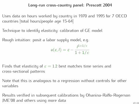
Long-run cross-country panel: Prescott 2004
Uses data on hours worked by country in 1970 and 1995 for 7 OECDcountries [total hours/people age 15-64]
Technique to identify elasticity: calibration of GE model
Rough intuition: posit a labor supply model, e.g.
u(c , l) = c − l1+1/ε
1+ 1/ε
Finds that elasticity of ε = 1.2 best matches time series andcross-sectional patterns
Note that this is analogous to a regression without controls for othervariables
Results verified in subsequent calibrations by Ohanina-Raffo-RogersonJME’08 and others using more data
37 55

Raj Chetty () Labor Supply Harvard, Fall 2009 172 / 227

Reconciling Micro and Macro Estimates
Recent interest in reconciling micro and macro elasticity estimates (seeChetty-Guren-Manoli-Weber ’13)
Three potential explanations
a) Statistical Bias: culture differs in countries with higher tax rates[Alesina, Glaeser, Sacerdote 2005, Steinhauer 2018 for Swiss communitiesby language]
b) Macro-elasticity captures long-term response which could be largerthan short-term response (frictions, etc. Chetty ’12).
c) Other programs: retirement, education affect labor supply at beginningand end of working life (Blundell-Bozio-Laroque ’11) and child careaffecting mothers (Kleven JEP’14)
38 55

Blundell-Bozio-Laroque ’13
Strong evidence that variation in aggregate hours of work across countrieshappens among the young and the old: (a) schooling-work margin (b)presence of young children (for women), (c) early retirement
Serious cross-country time series analysis would require to put together abetter tax wedge by age groups which includes all those additional govtprograms [welfare, retirement, child care]
This has been done quite successfully in the case of retirement by series ofbooks by Gruber and Wise, Retirement around the world
⇒ Need to develop a more comprehensive international / time seriesdatabase of tax wedges by age and family types
39 55

Long-term effects: Evidence from the Israeli Kibbutz
Abramitzky ’15 book based on series of academic papers
Kibbutz are egalitarian and socialist communities in Israel, thrived foralmost a century within a more capitalist society
1) Social sanctions on shirkers effective in small communities with limitedprivacy
2) Deal with brain drain exit using communal property as a bond
3) Deal with adverse selection in entry with screening and trial period
4) Perfect sharing in Kibbutz has negative effects on high school studentsperformance but effect is small in magnitude (concentrated among kids withlow education parents)
40 55

Long-term effects: Evidence from the Israeli Kibbutz
Abramitzky-Lavy ECMA’14 show that high school students study harderonce their kibbutz shifts away from equal sharing
Uses a DD strategy: pre-post reform and comparing reform Kibbutz tonon-reform Kibbutz. Finds that
1) Students are 3% points more likely to graduate
2) Students are 6% points more likely to achieve a matriculation certificatethat meets university entrance requirements
3) Students get an average of 3.6 more points in their exams
Effect is driven by students whose parents have low schooling; larger formales; stronger in kibbutz that reformed to greater degree
41 55

Culture of Welfare across Generations
Conservative concern that welfare promotes a culture of dependency: kidsgrowing up in welfare supported families are more likely to use welfare
Correlation in welfare use across generations is obviously not necessarilycausal
Dahl, Kostol, Mogstad QJE’2014 analyze causal effect of parental use ofDisability Insurance (DI) on children use (as adults) of DI in Norway
Identification uses random assignment of judges to denied DI applicantswho appeal [some judges are severe, some lenient]
Find evidence of causality: parents on DI increases odds of kids on DI overnext 5 years by 6 percentage points
Mechanism seems to be learning about DI availability rather than reduced stigmafrom using DI [because no effect on other welfare programs use]
42 55

����� ������� �� � � �� � ��� ����� � ����� ��� ������� �� � � �� ����� ������ ������� �� ������� ��
���� ��� ����� �� ����� ��� ���� ������� � ��� �� ����� � ��� �� ��� �� ������� � �������� ����
����� ��� ������ � � �� �� ��� ������ ��� ��� �� �� ������ �������� �� �� � � � � ����� ����� ��
�� ��!� ��� ��� ����� ������� � ��� ������ � ����� ������� � � �����"��� ��� ##$ �� ����� ������ ��
� ����� � �� %� � ����� ��� �������� � �����"��� ��� %$ � �� �� � ����� ����
������ �� ��� � ����� �������� � ������� ������ ������ ��� �������� �������� � ����
0.0
5.1
.15
.2.2
5.3
.35
Par
ent a
llow
ance
rat
e
02
46
810
Den
sity
(%
)
.01 .05 .09 .13 .17 .21 .25 .29 .33Judge leniency (leave−out mean judge allowance rate)
(A) First stage
.015
.02
.025
.03
.035
.04
.045
Chi
ld D
I rat
e in
yea
r 5
02
46
810
Den
sity
(%
)
.01 .05 .09 .13 .17 .21 .25 .29 .33Judge leniency (leave−out mean judge allowance rate)
(B) Reduced form
������ �������� ����� ������ ��� �� ���� � ��� ���� �� ��� ����� ������ �� ����� ������ �� ����� ��������� ���� �� ��� ! ���
��� ��� �� ����"# $���� ��� �%��! ����&����� �'���&� ���� ��� (� ��)���� *�����# +���� �,"- ���� ���� �� � ����� ������ ���������� ��
���� �� �� ��������� �� *���� ��������# +���� ��"- ���� ���� �� � ����� ������ ���������� �� ����� �� ����� �� ���� ���� .� *����
�������� �������# ,�� ����������� ������� ����� �� ���� �� ���� ��� ���� ��� �������# $�� ��� ����� �� *���� �������� �� ����� ��
�� '��/������ �� '� � 0����� � � ��� '� �� �#�1 �2������ ���� �� ����"#
&��� ' ���� �� �(�� �� ����� ������ � � ���� )� ������� �� �� ��� ����� �� � *�"���� �����
� �� +�� � ��� �,�� �� -./� ���� � ��� � ����� ����� ��������� �� �� ��� ���� �� ������� �����
����� ������� ��� ���� �� ������� �� � �� ��� ������� �������� � ��� ������ �������� �� ��
����� � ������ ' �� ����� ��� ��� ������� � �� �����)� ������� �� � � � ��� ����� �� ������� ��
� � � ����� �� ����� ��� ��� ������� � �� ��������� � �� ���� )� ���� �� ������� &��� 0 ��� �
�� ������� ���� �(�� �� � ���� )� ����� ������ ������� ����� ���� �����)� 12 ��� ����� ��� ����
���� � ����� ����� ���������� ��� �����)� 12 �� � �� ��� ������� �������� � �� ������ ������� ��
���� '����"��� ��� � �� � ���� ����� �� ������� ���� ���� � ��� � ���� ����� � ��� ����� -������
������� 3��%� �� �� � ����� ���/ ��� ������ �� � ��� ����� � � 12 +�� ����� �� ��� ���� �� �� �� ��� ��
� � ������� ���� ����� �� ������� ���� ���� � ��� � ���� ����� ���� ����� -������ ������� 3 �##�
�� %� � ����� ���/�
�
Source: Dahl, Kostol, Mogstad (2013)

REFERENCES
Abramitzky, Ran The Mystery of the Kibbutz: How Socialism Succeeded,Princeton: Princeton University Press, 2015 (in preparation) (web)
Abramitzky, Ran and Victor Lavy, 2014 “How Responsive is Investment inSchooling to Changes in Redistributive Policies and in Returns?”, Econometrica,82(4), 1241-1272 (web)
Alesina, A., E. Glaeser, and B. Sacerdote “Work and Leisure in the U.S. andEurope: Why So Different?”, NBER Macroeconomics Annual 2005. (web)
Ashenfelter, O. and M. Plant “Non-Parametric Estimates of the Labor SupplyEffects of Negative Income Tax Programs”, Journal of Labor Economics, Vol. 8, 1990,396-415. (web)
Bachas, Pierre and Mauricio Soto. “Not(ch) Your Average Tax System: CorporateTaxation Under Weak Enforcement,” World Bank Policy Research Working Paper8524, 2018. (web)
43 55

Bastani, Spencer and Hakan Selin, “Bunching and non-bunching at kink points ofthe Swedish tax schedule,” Journal of Public Economics, 109, 2014, 36-49. (web)
Bertrand, M., E. Duflo and S. Mullainhatan “How Much Should we TrustDifferences-in-Differences Estimates?”, Quarterly Journal of Economics, Vol. 119,2004, 249-275. (web)
Best, Michael and Henrik Kleven “Housing Market Responses to TransactionTaxes: Evidence from Notches and Stimulus in the UK,” Review of EconomicStudies 2017 forthcoming (web)
Bianchi, M., B. R. Gudmundsson, and G. Zoega. 2001. “Iceland’s Natural Experimentin Supply-Side Economics,” American Economic Review, 91(5), 1564-79. (web)
Bitler, M. J. Gelbach and H. Hoynes “What Mean Impacts Miss: DistributionalEffects of Welfare Reform Experiments”, American Economic Review, Vol. 96, 2006,988-1012. (web)
Bitler, M. and H. Hoynes “The State of the Safety Net in the Post-Welfare ReformEra” Brookings Papers on Economic Activity Fall 2010, 71-127 (web)
44 55

Blau, F. and L. Kahn “Changes in the Labor Supply Behavior of Married Women:1980-2000”, Journal of Labor Economics, Vol. 25, 2007, 393-438. (web)
Blomquist, S. “Restrictions in labor supply estimation: Is the MaCurdy critiquecorrect?”, Economics Letters, Vol. 47, 1995, 229-235 (web)
Blomquist, Soren and Whitney Newey “The Bunching Estimator Cannot Identifythe Taxable Income Elasticity”, NBER Working Paper No. 24136. (web)
Blundell, Richard, Antoine Bozio, and Guy Laroque. 2013. “Extensive and IntensiveMargins of Labour Supply: Work and Working Hours in the US, UK and France,”Fiscal Studies, 34(1), 1-29 (web)
Blundell, R., A. Duncan and C. Meghir “Estimating Labor Supply Responses UsingTax Reforms”, Econometrica, Vol. 66, 1998, 827-862. (web)
Blundell, R. and T. MaCurdy “Labor supply: a review of alternative approaches”, inthe Handbook of Labor Economics, Vol. 3A, O. Ashenfelter and D. Card, eds.Amsterdam: Elsevier Science 1999. (web)
Brown, K. “The Link between Pensions and Retirement Timing: Lessons fromCalifornia Teachers”, Journal of Public Economics, 98, 2013, 1–14. 2007 (web)
45 55

Camerer, C., L. Babcock, G. Loewenstein and R. Thaler “Labor Supply of New YorkCity Cabdrivers: One Day at a Time”, Quarterly Journal of Economics, Vol. 112,1997, 407-441. (web)
Card, David, Raj Chetty, Martin Feldstein, and Emmanuel Saez “Expanding Accessto Administrative Data for Research in the United States,” White Paper for NSF10-069 call for papers on "Future Research in the Social, Behavioral, and EconomicSciences" September 2010. (web)
Card, D.,R. Chetty, and A. Weber, “Cash-on-Hand and Competing Models ofIntertemporal Behavior: New Evidence from the Labor Market”, Quarterly Journalof Economics, Vol. 122, 2007, 1511-1560. (web)
Card, David, and Dean R. Hyslop. 2005. “Estimating the Effects of a Time-LimitedEarnings Subsidy for Welfare-Leavers” Econometrica, 73(6), 1723-70. (web)
Cesarini, David, Erik Lindqvist, Matthew J. Notowidigdo, Robert Ostling. 2015 “TheEffect of Wealth on Individual and Household Labor Supply: Evidence fromSwedish Lotteries”, NBER Working Paper No. 21762. (web)
Chetty, R. “A New Method of Estimating Risk Aversion”, The American EconomicReview, Vol. 96, 2006, 1821-1834. (web)
46 55

Chetty, Raj. 2012. “Bounds on Elasticities with Optimization Frictions: A Synthesisof Micro and Macro Evidence on Labor Supply,” Econometrica 80(3), 969–1018.(web)
Chetty, R., Adam Guren, Day Manoli, and Andrea Weber. 2013 “Does IndivisibleLabor Explain the Difference between Micro and Macro Elasticities? AMeta-Analysis of Extensive Margin Elasticities”, NBER Macroeconomics Annual,University of Chicago Press, 27(1), 1–56. (web)
Chetty, R., J. Friedman, T. Olsen and L. Pistaferri “Adjustment Costs, FirmsResponses, and Micro vs. Macro Labor Supply Elasticities: Evidence from DanishTax Records”, Quarterly Journal of Economics, 126(2), 2011, 749-804. (web)
Chetty, R., J. Friedman and E. Saez “Using Differences in Knowledge AcrossNeighborhoods to Uncover the Impacts of the EITC on Earnings”, AmericanEconomic Review, 2013, 103(7), 2683-2721 (web)
Chetty, R. and E. Saez “Teaching the Tax Code: Earnings Responses to anExperiment with Recipients”, American Economic Journal: Applied Economics 5(1),2013, 1-31. (web)
47 55

Crawford, V. and J. Meng “New York City Cabdrivers’ Labor Supply Revisited:Reference-Dependence Preferences with Rational-Expectations Targets for Hoursand Income”, University of California at San Diego, Economics Working PaperSeries: 2008-03, 2008. (web)
Dahl, Gordon B., Andreas Ravndal Kostol, Magne Mogstad “Family WelfareCultures” Quarterly Journal of Economics, 129(4), 2014, 1711-52 (web)
Davis, J. and M. Henrekson, “Tax Effects on Work Activity, Industry Mix andShadow Economy Size: Evidence from Rich Country Comparisons”, in R.Gomez-Salvador, A. Lamo, B. Petrongolo, M. Ward and E. Wasmer eds., LabourSupply and Incentives to Work in Europe, 2005, 44-104. (web)
Devereux, Michael P, Li Liu and Simon Loretz. 2014. "The Elasticity of CorporateTaxable Income: New Evidence from UK Tax Records." American Economic Journal:Economic Policy, 6(2): 19-53. (web)
Einav, Liran, Amy Finkelstein, Paul Schrimpf “The Data Revolution and EconomicAnalysis’, NBER Working Paper 19035, 2013. (web)
Einav, Liran and Jonathan Levin “The Data Revolution and Economic Analysis”,NBER Working Paper No. 19035, 2013 (web)
48 55

Eissa, N. and H. Hoynes “Taxes and the labor market participation of marriedcouples: the earned income tax credit”, Journal of Public Economics, Vol. 88, 2004,1931-1958. (web)
Eissa, N. and J. Liebman “Labor Supply Response to the Earned Income TaxCredit”, Quarterly Journal of Economics, Vol. 111, 1996, 605-637. (web)
Farber, H. “Is Tomorrow Another Day? The Labor Supply of New York City CabDrivers”, Journal of Political Economy, Vol. 113, 2005, 46-82. (web)
Farber, H. “Reference-Dependent Preferences and Labor Supply: The Case of NewYork City Taxi Drivers”, The American Economic Review, Vol. 98, 2008, 1069-1082.(web)
Fehr, E. and L. Goette “Do Workers Work More if Wages Are High? Evidence froma Randomized Field Experiment”, American Economic Review, Vol. 97, 2007,298-317. (web)
Friedberg, L. “The Labor Supply Effects of the Social Security Earnings Test”,Review of Economics and Statistics, Vo. 82, 2000, 48-63. (web)
49 55

Greenberg, D. and H. Hasley, “Systematic Misreporting and Effects of IncomeMaintenance Experiments on Work Effort: Evidence from the Seattle-DenverExperiment”, Journal of Labor Economics, Vol. 1, 1983, 380-407. (web)
Hausman, J. “Stochastic Problems in the Simulation of Labor Supply”, NBERWorking Paper No. 0788, 1981. (web)
Hausman, J. “Taxes and Labor Supply”, in A. Auerbach and M. Feldstein, eds,Handbook of Public Finance, Vol I, North Holland 1987. (web)
Heckman, J. “What Has Been Learned About Labor Supply in the Past TwentyYears?”, American Economic Review, Vol. 83, 1993, 116-121. (web)
Heckman, J. and M. Killingsworth “Female Labor Supply: A Survey” Handbook ofLabor Economics, Vol. I, Chapter 2, 1986. (web)
Imbens, G.W., D.B. Rubin and B.I. Sacerdote “Estimating the Effect of UnearnedIncome on Labor Earnings, Savings, and Consumption: Evidence from a Surveyof Lottery”, American Economic Review, Vol. 91, 2001, 778-794. (web)
50 55

Jakobsen, Kristian, Katrine Jakobsen, Henrik Kleven and Gabriel Zucman. 2018.Wealth Accumulation and Wealth Taxation: Theory and Evidence from DenmarkÓNBER working paper No. 24371. (web)
Jones, Damon “Information, Inertia and Public Benefit Participation: ExperimentalEvidence from the Advance EITC and 401(k) Savings“, AEJ: Applied Economics, Vol.2, 2010, 147-163. (web)
Keane, Michael “Labor Supply and Taxes: A Survey?”, Journal of EconomicLiterature, Vol. 49(4), 2011, 961-1075. (web)
Kleven, Henrik “How Can Scandinavians Tax So Much?”, Journal of EconomicPerspectives 28(4), 77-98, 2014 (web)
Kleven, Henrik “Taxation and Labor Force Participation: The EITCReconsidered”, October 2018 frames (web)
Kleven, Henrik “Taxation and Labor Force Participation: The EITC Reconsidered”,October 2018 frames (web)
Kleven, Henrik “Bunching”, Annual Review of Economics, 8, 2016, 435-464.(web)
51 55

Kleven, Henrik and Mazhar Waseem, 2013“Using notches to uncover optimizationfrictions and structural elasticities: Theory and evidence from Pakistan”, QuarterlyJournal of Economics 2013, 669-723. (web)
Kline, Patrick and Melissa Tartari, 2016. "Bounding the Labor Supply Responsesto a Randomized Welfare Experiment: A Revealed Preference Approach," AmericanEconomic Review, 106(4), 972-1014. (web)
Kopczuk, Wojciech and David J. Munroe, 2015 “Mansion Tax: The Effect of TransferTaxes on the Residential Real Estate Market”, American Economic Journal:Economic Policy, 7(2), 214-57 (web)
Liebman, J. and R. Zeckhauser “Schmeduling”, Harvard University working paper,October 2004. (web)
Londono-Velez, Juliana and Javier Avila. “Can Wealth Taxation Work in DevelopingCountries? Quasi-Experimental Evidence from Colombia", UC Berkeley workingpaper, 2018. (web)
MaCurdy, T. “An Empirical Model of Labor Supply in a Life-Cycle Setting”, Journalof Political Economy, Vol. 89, 1981, 1059-1085. (web)
52 55

MaCurdy, T. “A Simple Scheme for Estimating an Intertemporal Model of LaborSupply and Consumption in the Presence of Taxes and Uncertainty”, InternationalEconomic Review, Vol. 24, 1983, 265-289. (web)
MaCurdy, T., D. Green and H. Paarsch “Assessing Empirical Approaches forAnalyzing Taxes and Labor Supply” Journal of Human Resources, Vol. 25, 1990,415-490. (web)
Meyer, B. and D. Rosenbaum “Welfare, the Earned Income Tax Credit, and theLabor Supply of Single Mothers”, Quarterly Journal of Economics, Vol. 116, August2001, 1063-1114. (web)
Meyer, B. and X. Sullivan “The effects of welfare and tax reform: the materialwell-being of single mothers in the 1980s and 1990s”, Journal of Public Economics,Vol. 88, 2004, 1387-1420. (web)
Moffitt, R. “Welfare Programs and Labor Supply”, in A. Auerbach and M. Feldstein,Handbook of Public Economics, Volume 4, Chapter 34, Amsterdam: North Holland,2003. (web)
53 55

Mortenson, Jacob A. and Andrew Whitten. 2016. “Bunching to Maximize TaxCredits: Evidence from Kinks in the U.S. Tax Schedule”, OTA-JCT working paper(web)
Mroz, T. “The Sensitivity of An Empirical Model of Married Women’s Hours of Workto Economic and Statistical Assumptions”, Econometrica, Vol. 55, 1987, 765-799.(web)
Munnell, A., Lessons from the income maintenance experiments : proceedings of aconference held at Melvin Village, New Hampshire, September 1986. Boston:Federal Reserve Bank of Boston, 1986. (web)
Nichols, Austin and Jesse Rothstein 2015. “The Earned Income Tax Credit”,forthcoming in Volume on US Transfer Programs edited by R. Moffitt (web)
Oettinger, G. “An Empirical Analysis of the Daily Labor Supply of StadiumVendors”, Journal of Political Economy, Vol. 107, 1999, 360-392. (web)
Ohanian, L., A. Raffo, and R. Rogerson “Long-Term Changes in Labor Supply andTaxes: Evidence from OECD Countries, 1956-2004”, Journal of MonetaryEconomics, Vol. 55, 2008, 1353-1362. (web)
54 55

Pencavel, J. “Labor Supply of Men: A Survey”, Handbook of Labor Economics, vol.1, chapter 1, 1986. (web)
Pencavel, J. “A Cohort Analysis of the Association between Work Hours and Wagesamong Men”, The Journal of Human Resources, Vol. 37, 2002, 251-274. (web)
Prescott, E. “Why Do Americans Work So Much More Than Europeans?”, NBERWorking Paper No. 10316, 2004, published in FRB Minneapolis - QuarterlyReview, 2004, 28(1), 2-14. (web)
Prescott, E. “Nobel Lecture: The Transformation of Macroeconomic Policy andResearch”, Journal of Political Economy, 114, 2006, 203-235. (web)
Ramey, Valerie A. and Neville Francis, 2009. “A Century of Work and Leisure,”American Economic Journal: Macroeconomics, 1(2), 189-224. (web)
Rees, A. “An Overview of the Labor-Supply Results”, The Journal of HumanResources, Vol. 9, 1974, 158-180. (web)
Rees-Jones, Alex and Dmitry Taubinsky. 2016 “Measuring “Schmeduling” ”, NBERWorking Paper No. 22884.(web)
55 55

Rogerson, R. and J. Wallenius “Micro and Macro Elasticities in a Life Cycle Modelwith Taxes”, Journal of Economic Theory, Vol. 144, 2009, 2277-2292. (web)
Rothstein, J. ‘Is the EITC as Good as an NIT? Conditional Cash Transfers and TaxIncidence.” American Economic Journal: Economic Policy 2 (1), February 2010,177-208. (web)
Saez, E. “Do Taxpayers Bunch at Kink Points?”, NBER Working Paper No. 7366,1999. (web)
Saez, E. “Do Taxpayers Bunch at Kink Points?”, AEJ: Economic Policy, Vol. 2,2010, 180-212. (web)
Saez, E., J. Slemrod, and S. Giertz “The Elasticity of Taxable Income with Respectto Marginal Tax Rates: A Critical Review”, Journal of Economic Literature 50(1),2012, 3-50. (web)
Seim, David. 2017. "Behavioral Responses to an Annual Wealth Tax: Evidence fromSweden", American Economic Journal: Economic Policy, 9(4), 395-421. (web)
Steinhauer, Andreas. 2018 “Working Moms, Childlessness, and Female Identity”,CEPR Discussion Paper No. 12929.(web)
56 55


