TD-SCDMA Relay Networks Sun Yan Submitted for the Degree of Doctor of Philosophy Supervisor: Prof. Laurie Cuthbert School of Electronic Engineering and Computer Science Queen Mary, University of London February 2009
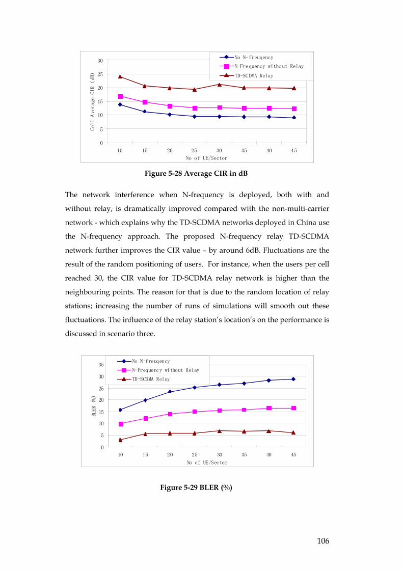
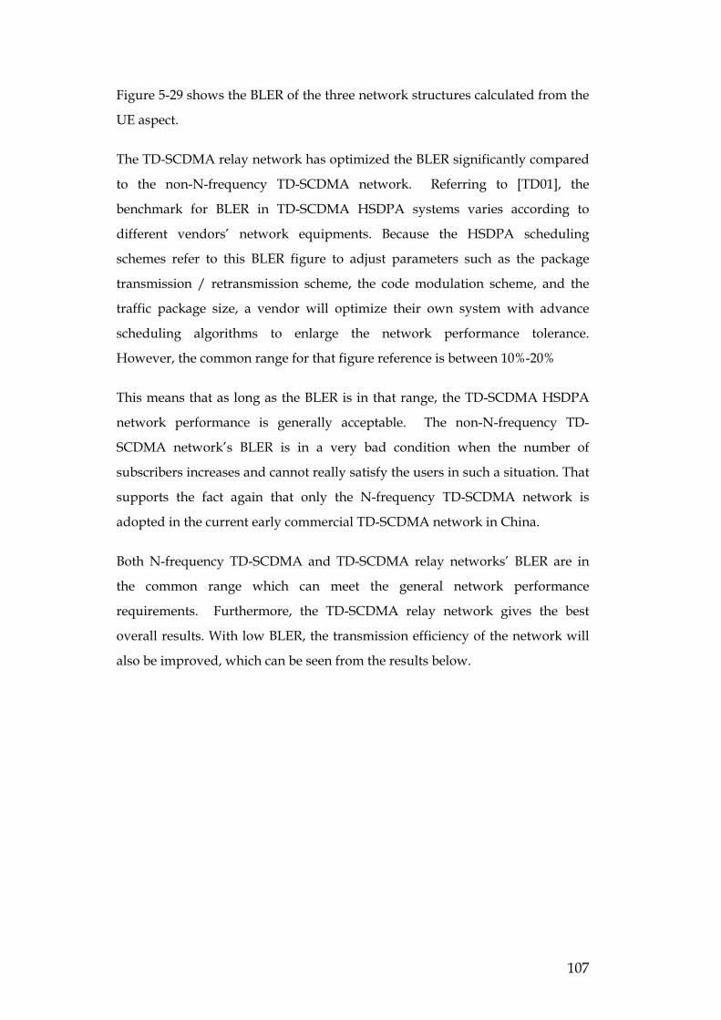
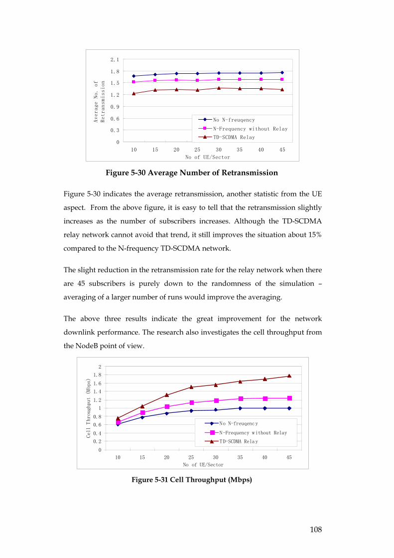
Transcript
TD-SCDMA Relay Networks
Sun Yan
Submitted for the Degree of Doctor of Philosophy
Supervisor: Prof. Laurie Cuthbert
School of Electronic Engineering and Computer Science Queen Mary, University of London
February 2009
2
To my beloved Mum and Dad
3
Abstract
When this research was started, TD-SCDMA (Time Division Synchronous Code
Division Multiple Access) was still in the research/development phase, but
now, at the time of writing this thesis, it is in commercial use in 10 large cities in
China including Beijing and Shang Hai. In all of these cities HSDPA is enabled.
The roll-out of the commercial deployment is progressing fast with installations
in another 28 cities being underway now.
However, during the pre-commercial TD-SCDM trail in China, which started
from year 2006, some interference problems have been noticed especially in the
network planning and initialization phases. Interference is always an issue in
any network and the goal of the work reported in this thesis is to improve
network coverage and capacity in the presence of interference.
Based on an analysis of TD-SCDMA issues and how network interference arises,
this thesis proposes two enhancements to the network in addition to the
standard N-frequency technique. These are (i) the introduction of the concentric
circle cell concept and (ii) the addition of a relay network that makes use of
other users at the cell boundary. This overall approach not only optimizes the
resilience to interference but increases the network coverage without adding
more Node Bs.
Based on the cell planning parameters from the research, TD-SCDMA HSDPA
services in dense urban area and non-HSDPA services in rural areas were
simulated to investigate the network performance impact after introducing the
relay network into a TD-SCDMA network.
The results for HSDPA applications show significant improvement in the TD-
SCDMA relay network both for network capacity and network interference
aspects compared to standard TD-SCDMA networks. The results for non-
HSDPA service show that although the network capacity has not changed after
adding in the relay network (due to the code limitation in TD-SCDMA), the
TD-SCDMA relay network has better interference performance and greater
coverage.
4
Acknowledgement
First I would like to express my biggest and sincerest “thanks” to my supervisor,
Prof Laurie Cuthbert for his understanding, support, encouragement and
personal guidance during these years, especially as he flew from London to
Beijing many times to supervise my research on the spot as well as spending a
lot of time on remote supervision. Without his continuous help I would not
have completed my PhD study and this thesis would not exist.
I would like to thank my ex-colleagues in Siemens Ltd. China as well. Although
this research work has been done entirely by myself, their valuable sharing of
knowledge and rich working experiences did help me cope with the part-time
PhD distance research. Without their understanding and support, I would not
have finally finished the research work without affecting the quality of my daily
job.
Also I would like to express my gratitude to the Wireless Signal Processing and
Network Lab at Beijing University of Posts and Telecommunications (BUPT)
who provided me the basic simulation materials and shared their advice
generously.
Furthermore I would like to thank all those in the Department of Electronic
Engineering, at Queen Mary, who have given me valuable advice and support,
either locally during my periodic short visits or remotely when I was in China.
Finally, my love and gratitude from my heart go to my dearest parents; their
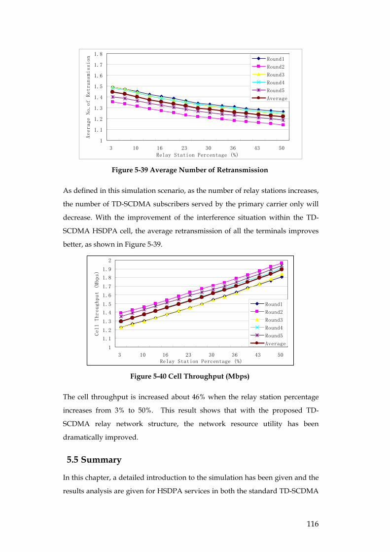
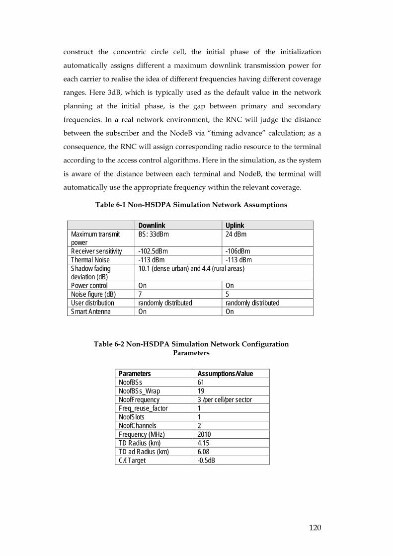
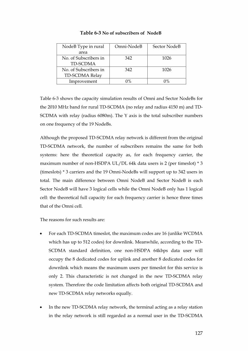
6.2 Simulation Result and Analysis of 64K Data Application················126 6.2.1 Capacity analysis ·········································································126 6.2.2 Average noise rise analysis ····························································128
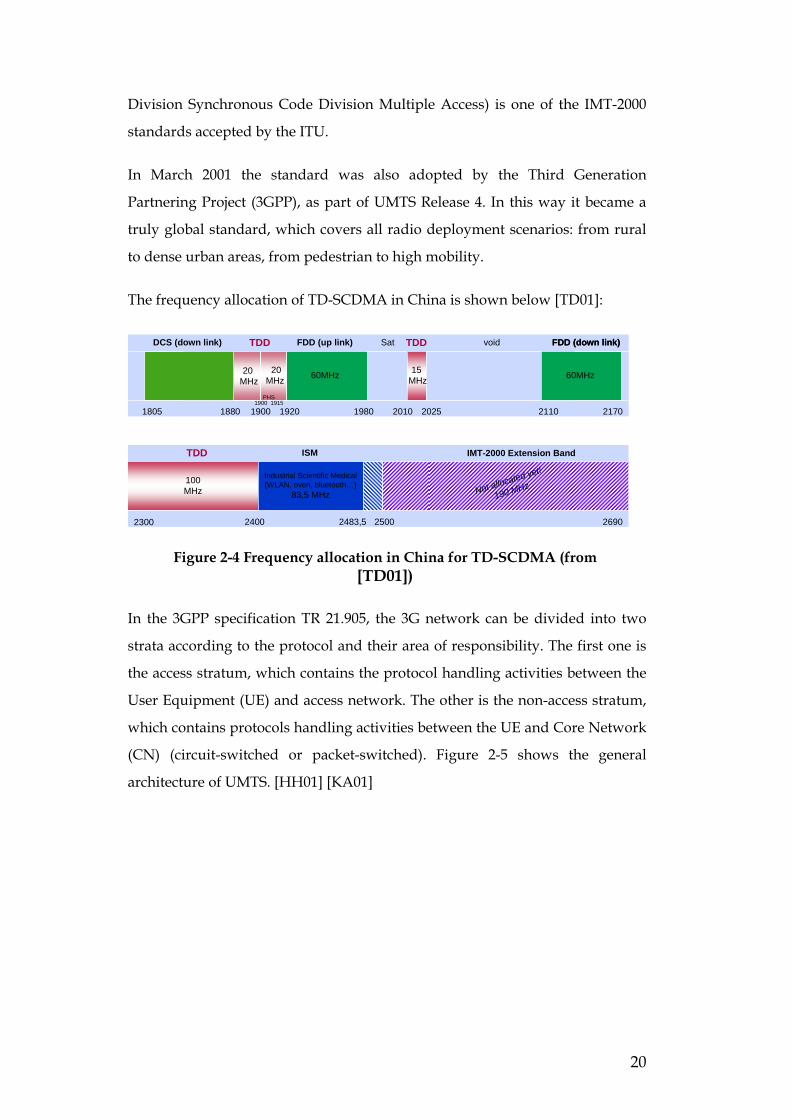
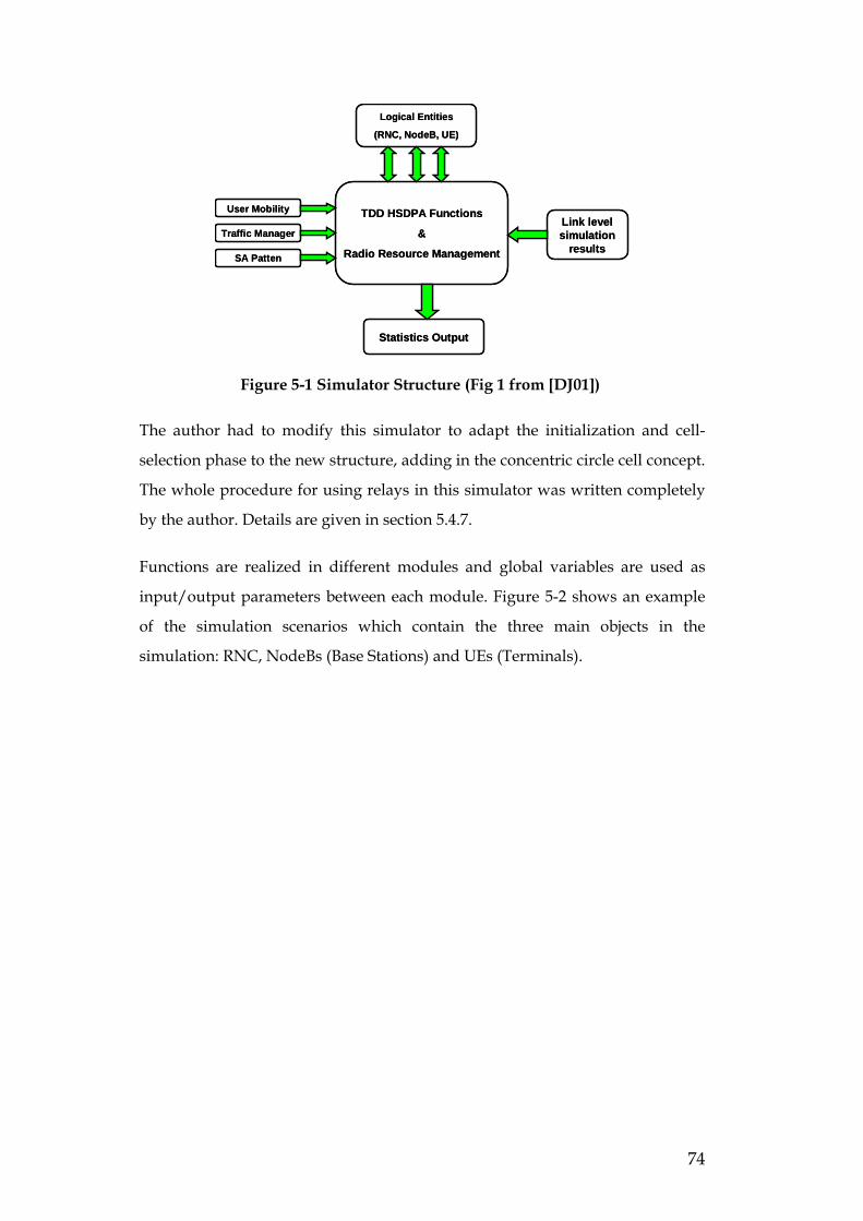
Figure 2-4 Frequency allocation in China for TD-SCDMA (from [TD01])
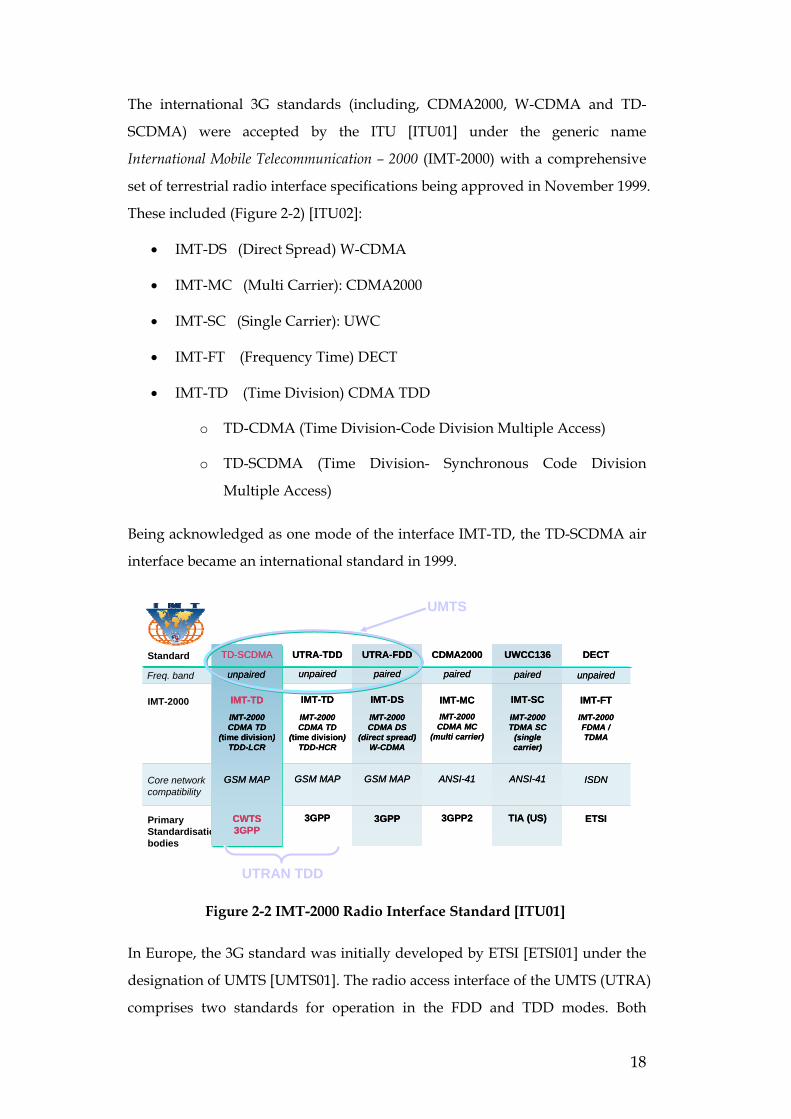
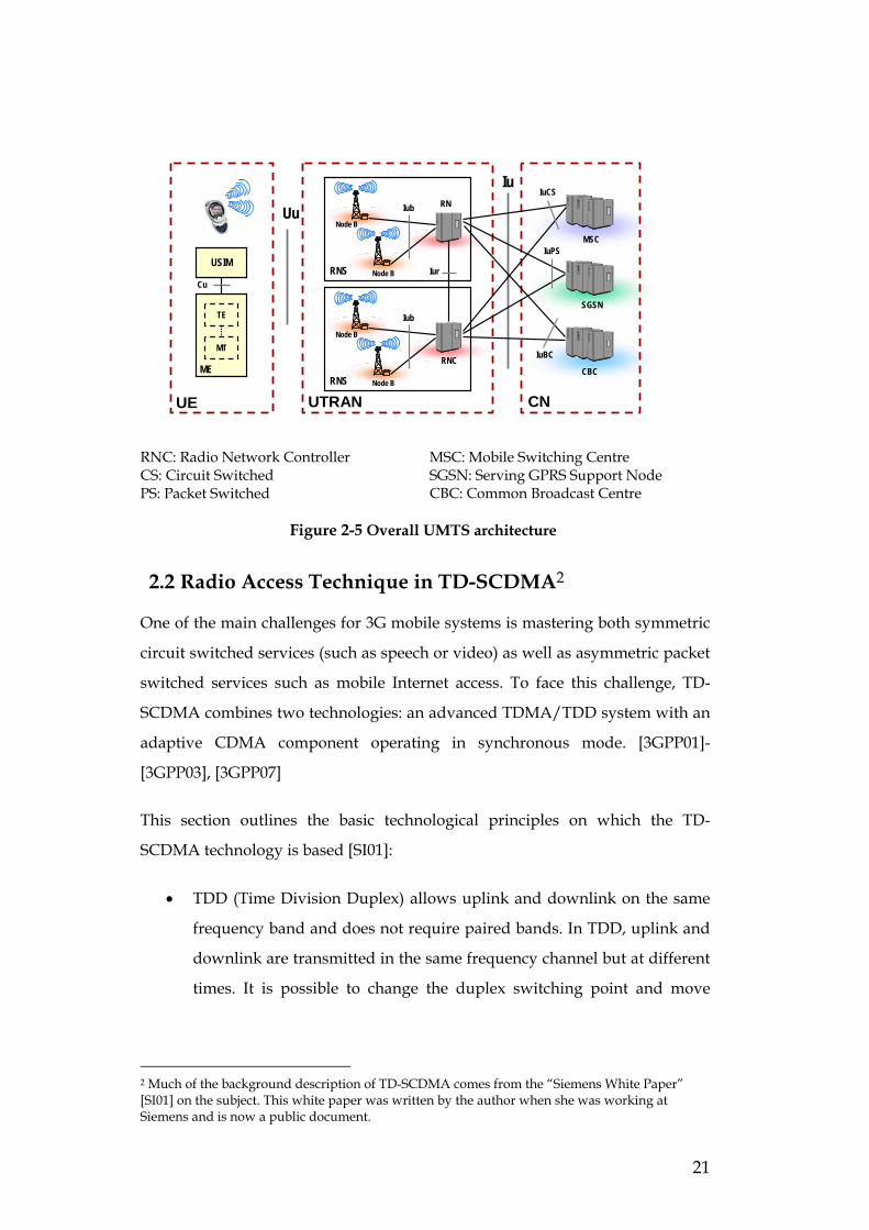
In the 3GPP specification TR 21.905, the 3G network can be divided into two
strata according to the protocol and their area of responsibility. The first one is
the access stratum, which contains the protocol handling activities between the
User Equipment (UE) and access network. The other is the non-access stratum,
which contains protocols handling activities between the UE and Core Network
(CN) (circuit-switched or packet-switched). Figure 2-5 shows the general
architecture of UMTS. [HH01] [KA01]
21
UE
USIM
TE
MT
ME
Cu
UTRAN CN
Uu
Iu
RNS Node B
RNIub
Node B
RNS Node B
RNC
Iub
Node B
Iur
IuPS
SGSN
MSC
CBC
IuCS
IuBC
RNC: Radio Network Controller CS: Circuit Switched PS: Packet Switched
MSC: Mobile Switching Centre SGSN: Serving GPRS Support Node CBC: Common Broadcast Centre
Figure 2-5 Overall UMTS architecture
2.2 Radio Access Technique in TD-SCDMA2
One of the main challenges for 3G mobile systems is mastering both symmetric
circuit switched services (such as speech or video) as well as asymmetric packet
switched services such as mobile Internet access. To face this challenge, TD-
SCDMA combines two technologies: an advanced TDMA/TDD system with an
adaptive CDMA component operating in synchronous mode. [3GPP01]-
[3GPP03], [3GPP07]
This section outlines the basic technological principles on which the TD-
SCDMA technology is based [SI01]:
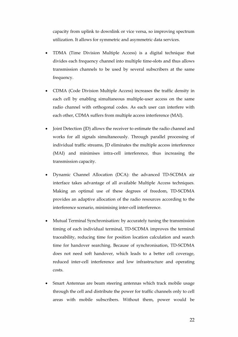
• TDD (Time Division Duplex) allows uplink and downlink on the same
frequency band and does not require paired bands. In TDD, uplink and
downlink are transmitted in the same frequency channel but at different
times. It is possible to change the duplex switching point and move
2 Much of the background description of TD-SCDMA comes from the “Siemens White Paper” [SI01] on the subject. This white paper was written by the author when she was working at Siemens and is now a public document.
22
capacity from uplink to downlink or vice versa, so improving spectrum
utilization. It allows for symmetric and asymmetric data services.
• TDMA (Time Division Multiple Access) is a digital technique that
divides each frequency channel into multiple time-slots and thus allows
transmission channels to be used by several subscribers at the same
frequency.
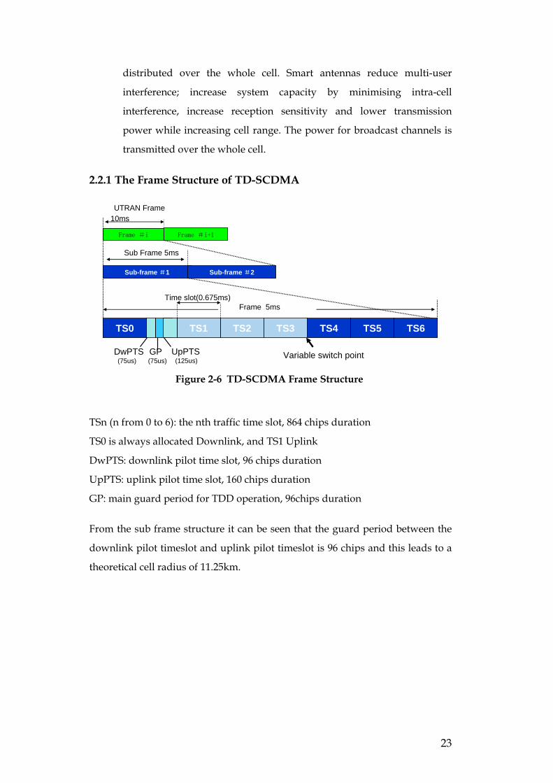
• CDMA (Code Division Multiple Access) increases the traffic density in
each cell by enabling simultaneous multiple-user access on the same
radio channel with orthogonal codes. As each user can interfere with
each other, CDMA suffers from multiple access interference (MAI).
• Joint Detection (JD) allows the receiver to estimate the radio channel and
works for all signals simultaneously. Through parallel processing of
individual traffic streams, JD eliminates the multiple access interference
(MAI) and minimises intra-cell interference, thus increasing the
transmission capacity.
• Dynamic Channel Allocation (DCA): the advanced TD-SCDMA air
interface takes advantage of all available Multiple Access techniques.
Making an optimal use of these degrees of freedom, TD-SCDMA
provides an adaptive allocation of the radio resources according to the
CDMA (Code Division Multiple Access) and SDMA (Space Division Multiple
Access). Making an optimal use of these degrees of freedom, TD-SCDMA
provides an optimal and adaptive allocation of the radio resources according to
the interference scenario, minimising intercell interference.
The following three different methods of DCA are used:
• Time Domain DCA (TDMA operation): Traffic is dynamically allocated
to the least interfered timeslots.
• Frequency Domain DCA (FDMA operation): Traffic is dynamically
allocated to the least interfered radio carrier (3 available 1.6 MHz radio
carriers in 5MHz band).
• Code Domain DCA (CDMA operation): Traffic is dynamically allocated
to the least interfered codes (16 codes per timeslot per radio carrier).
30
Energy
Tim
e
FDMA
Frequency
CDMA
TDMA
TD-SCDMA minimises Intercell Interference by dynamically allocating least interfered resources.
Figure 2-13 Dynamic Channel Allocation
2.2.6 Terminal Synchronisation
Like all TDMA systems TD-SCDMA needs an accurate synchronisation
between mobile terminal and NodeB [HH02]. This synchronisation becomes
more complex through the mobility of the subscribers, because they can stay at
varying distances from the NodeB and their signals have different propagation
times.
A precise timing advance in the handset during transmission eliminates those
varying time delays. In order compensate these delays and avoid collisions of
adjacent time slots, the mobile terminals advance the time-offset between
reception and transmission so that the signals arrive frame-synchronous at the
NodeB (Figure 2-14).
UplinkDownlinkTimeDistance
from Base Station
Near
Far
Timing Advance
Propagation Delay
Figure 2-14 Uplink Synchronization
31
The effect of this precise synchronisation of the signals arriving at the NodeB
leads to a significant improvement in multi user joint detection.
By implementing the synchronous deployment, the terminal traceability is
improved and the time for position location calculations is sensibly reduced. In
addition, in a synchronous system, the mobile terminal when non-actively
receiving or transmitting (idle timeslots) can perform measurements of the radio
link quality of the neighbouring NodeBs. This results in reduced search times
for handover searching (both intra- and inter-frequency searching), which
produces a significant improvement in standby time.
2.2.7 N-Frequency in TD-SCDMA
As defined in 3GPP, each cell in UMTS networks will contain only one carrier;
for WCDMA a 10MHz frequency band (uplink and downlink) is used while
TD-SCDMA uses 1.6MHz.
Each cell can only have one carrier
N carriers in the same sector means N cells
UE will be covered by multiple cell broadcast signals with equivalent strength
Figure 2-15 Without N-frequency Cell
The N-frequency concept was first introduced in China through the Chinese
standardisation body CCSA [CCSA01]-[CCSA07] and was later proposed to
3GPP. In the N-frequency network, each cell can have up to 12 carriers. All the
carriers within one cell are identified by one cell ID. When establishing the cell,
one carrier is configured as primary frequency and the rest are configured as
secondary frequency (ies).
Cell ACell ACell BCell B
Cell C Cell C
32
All carriers will be configured with the same Midamble3 code ID, scrambling
code ID and the N-frequency cell should have a unified uplink downlink
switching point. The reason is that all the carriers’ signals within one cell are
transmitted by one set of smart antennas and the smart antenna system can
only perform transmit or receive activity at one time. All the control channels
are configured on the primary frequency and TS0 on any secondary frequency
is not used by the network. Each individual UE can only work on one carrier at
one time under the current N-frequency concept.
TS0
Dw
PTSG
PU
pPTS TS1 TS2 TS3 TS4 TS5 TS6
GP
UpPTS TS1 TS2 TS3 TS4 TS5 TS6
GP
UpPTS TS1 TS2 TS3 TS4 TS5 TS6
Primary frequency
Secondary frequency1
Secondary frequency2
Not U
sedNot U
sed
Figure 2-16 N-frequency Cell Structure
When a UE camps on a cell, it firstly listens to the primary frequency for
broadcast messages. After successful access, the network will assign the traffic
channel to the particular UE according to the radio resource availability and
radio environment conditions. During the handover procedure, the terminal
will synchronize the primary carrier of the target cell from the serving carrier
directly; no matter whether it is primary or secondary carrier. The target cell
will allocate the dedicate channel to this incoming handover terminal on any of
the suitable carriers according to the network’s radio resource management
scheme. This research will not cover this radio resource management algorithm.
3 A burst is the combination of two data parts: a midamble part and a guard period. The duration of a burst is one time slot. Several bursts can be transmitted at the same time from one transmitter. In this case, the data parts must use different OVSF channelization codes, but the same scrambling code. The midamble parts are either identically or differently shifted versions of a cell-specific basic midamble code.
33
Carrier 1Carrier 1
Carrier 2Carrier 2
Carrier 3Carrier 3
Cell ACell A
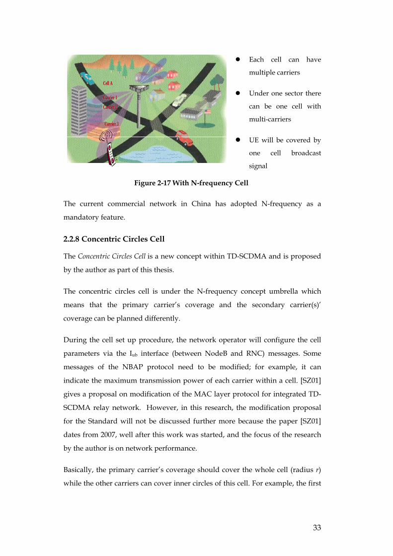
Each cell can have
multiple carriers
Under one sector there
can be one cell with
multi-carriers
UE will be covered by
one cell broadcast
signal
Figure 2-17 With N-frequency Cell
The current commercial network in China has adopted N-frequency as a
mandatory feature.
2.2.8 Concentric Circles Cell
The Concentric Circles Cell is a new concept within TD-SCDMA and is proposed
by the author as part of this thesis.
The concentric circles cell is under the N-frequency concept umbrella which
means that the primary carrier’s coverage and the secondary carrier(s)’
coverage can be planned differently.
During the cell set up procedure, the network operator will configure the cell
parameters via the Iub interface (between NodeB and RNC) messages. Some
messages of the NBAP protocol need to be modified; for example, it can
indicate the maximum transmission power of each carrier within a cell. [SZ01]
gives a proposal on modification of the MAC layer protocol for integrated TD-
SCDMA relay network. However, in this research, the modification proposal
for the Standard will not be discussed further more because the paper [SZ01]
dates from 2007, well after this work was started, and the focus of the research
by the author is on network performance.
Basically, the primary carrier’s coverage should cover the whole cell (radius r)
while the other carriers can cover inner circles of this cell. For example, the first
34
secondary carrier can cover the cell out to 2r/3 and the remaining secondary
carrier(s) can cover the cell to radius r/2.
Normally, the inner circle carriers will serve most of the traffic, and the outer
circle will maintain the service of those UEs that are at the edge of the cell. In
such a cell, the network can flexibly assign the radio resource to the UE
according to the UE’s position. The terminal will advance its timing when it
sends the signals to the base station in order to make sure all synchronized
transmission received by the NodeB from various terminals among the cell. The
NodeB will do the relevant location-based calculation to get the terminal’s
distance. Then the network can adaptively allocate the most suitable radio
resource for the terminals.
Advanced radio resource management algorithm adopted in the network will
balance the cell traffic and optimize the network efficiency. Meanwhile, the
more advanced algorithms of the smart antenna in such a concentric circle cell
will improve such aspects as the beam generation and the user location.
For the radio resource management algorithm, how to balance the traffic among
inner and outer circles, how to optimize the usage of each carrier are hot topics
as well but are outside the scope of this research.
2.2.9 Multi-carrier HSDPA in TD-SCDMA
HSDPA(High Speed Downlink Packet Access)is proposed by 3GPP in its R5
specification [3GPP06][3GPP09][3GPP12] to provide high data rate services in
the download direction in the packet domain and to enhance the bearer ability
of current 3G system. HSDPA is proposed both in TDD and FDD modes
[3GPP06]. Some advanced techniques, such as AMC (Adaptive Modulation
Coding) and HARQ (Hybrid Automatic Repeat reQuest), are adopted in
HSDPA and the fast packet scheduling function is located in the NodeB instead
of the RNC to shorten the round trip times.
In TDD HSDPA, the maximum data rate on one TD-SCDMA carrier is 2.8Mbps
with the asymmetric switching point 1:5 (UL: DL).
35
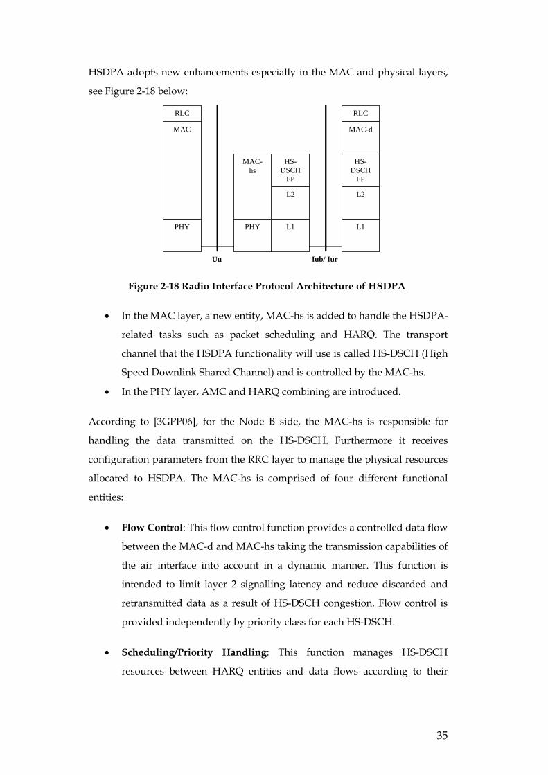
HSDPA adopts new enhancements especially in the MAC and physical layers,
see Figure 2-18 below:
L2
L1
HS-DSCH
FP
RLC
L2
L1
HS-DSCH
FP
Iub/ Iur
PHY
MAC
PHY
RLC
Uu
MAC-hs
MAC-d
Figure 2-18 Radio Interface Protocol Architecture of HSDPA
• In the MAC layer, a new entity, MAC-hs is added to handle the HSDPA-
related tasks such as packet scheduling and HARQ. The transport
channel that the HSDPA functionality will use is called HS-DSCH (High
Speed Downlink Shared Channel) and is controlled by the MAC-hs.
• In the PHY layer, AMC and HARQ combining are introduced.
According to [3GPP06], for the Node B side, the MAC-hs is responsible for
handling the data transmitted on the HS-DSCH. Furthermore it receives
configuration parameters from the RRC layer to manage the physical resources
allocated to HSDPA. The MAC-hs is comprised of four different functional
entities:
• Flow Control: This flow control function provides a controlled data flow
between the MAC-d and MAC-hs taking the transmission capabilities of
the air interface into account in a dynamic manner. This function is
intended to limit layer 2 signalling latency and reduce discarded and
retransmitted data as a result of HS-DSCH congestion. Flow control is
provided independently by priority class for each HS-DSCH.
• Scheduling/Priority Handling: This function manages HS-DSCH
resources between HARQ entities and data flows according to their
36
priority class. Based on status reports from associated uplink signalling
either new transmission or retransmission is determined.
• HARQ: One HARQ entity handles the hybrid ARQ functionality for one
user. One HARQ entity is capable of supporting multiple instances
(HARQ process) of stop and wait HARQ protocols. There shall be one
HARQ process per TTI.
• TFRI selection: Selection of an appropriate transport format and
resource combination for the data to be transmitted on HS-DSCH.
The MAC-hs, from the UE side, handles the following HSDPA specific
functions.
• HARQ: The HARQ entity is responsible for handling the HARQ
protocol and there is one HARQ process per HS-DSCH per TTI. The
HARQ functional entity handles all the tasks that are required for
hybrid ARQ.
• Reordering: The reordering entity organises received data blocks
according to the received TSN. Data blocks with consecutive TSNs are
delivered to higher layers upon reception. There is one reordering entity
for each priority class and MAC-identity configured at the UE.
In the HARQ protocol, the network operation performs the following actions:
• Scheduler: It includes scheduling all UEs within a cell, services priority
class queuing, determining the HARQ Entity and the queue to be served,
scheduling new transmissions and retransmissions:
• HARQ entity (one per UE): It includes priority class identifier setting,
transmission sequence number setting and HARQ process identifier
setting
• HARQ process: It includes New Data Indicator setting and processes
ACK/NACK from the receiver
37
Meanwhile the UE operation performs the following actions:
• HARQ entity: It mainly includes processing HARQ process identifiers
• HARQ process: It includes New Data Indicator processing, error
detection result processing, status report transmission and priority class
identifier processing
• Reordering entity: There is one re-ordering entity for each priority class
and transport channel configured at the UE. It performs the functions of
reordering of received data based on transmission sequence numbers
and forwarding data to higher layer
Now multi-carrier TD-SCDMA HSDPA is proposed in the CCSA (China
Communication Standard Association) which is the enhanced version of
single—carrier TDD HSDPA in 3GPP and much of the standardization work is
already completed. Moreover, the multi-carrier TD-SCDMA HSDPA supports
backward-compatible to both single-carrier TD-SCDMA HSDPA and N-
frequency TD-SCDMA network. So in the multi-carrier HSDPA concept, the
basic ideas are the same as in the principle of 3GPP HSDPA, the main difference
being that the terminal can work on multiple carriers at the same time in a
multi-carrier HSDPA system. Thus the maximum data rate in the multi-carrier
HSDPA system is n*2.8Mbps where n is the number of carriers. This is the
combination of N-frequency and HSDPA technologies.
The standards have been modified to include this combination and the
transmitting and receiving capability of the terminals needs to be enhanced
greatly. However, the big challenges to efficiently utilizing the network
resource are defining the proper channel resource scheduling solutions and re-
transmission schemes. With this multi-carrier HSDPA feature, higher bit rate
applications can be provided to end users - this is the evolution trend of TD-
SCDMA systems.
There are three types of channels newly defined in HSDPA systems: High
Speed Downlink Shared Channel (HS-DSCH), High Speed Shared Control
Channel (HS-SCCH) and High Speed Shared Information Channel (HS-SICH).
38
The HS-DSCH is the transport channel which is used to carry the HSDPA
related traffic data so the HS-DSCH is downlink only, while the HS-SCCH and
HS-SICH are physical channels used for transmitting the HSDPA signalling.
For the downlink, the UE should read the corresponding HS-SCCH channel to
get the HS-DSCH related information, such as Transmission Format and
Resource Indicator (TFRI), HARQ process identity and redundancy version.
Meanwhile the HS-SICH is an uplink control channel shared by UEs for
sending the HARD acknowledgement and the Channel Quality Indicator (CQI)
to the NodeB. In CQI, the information about the proposed modulation type,
recommended Transmission Block size are included.
Figure 2-19 gives one example of multi-carrier TD-SCDMA HSDPA resource
allocation. The HSDPA downlink control channels can only be configured on
the primary carrier and the TS0 timeslots on secondary carriers are not used. If
the UE supports multi-carrier receiving, the HSDPA resource of one particular
UE can be assigned on different codes, different timeslots and different carriers.
Primary frequency
Secondary frequency1
Secondary frequency2
TS0
Dw
PTS TS1
GP
UpPTS TS2 TS3 TS4 TS5 TS6
UL time slot
DL time slot
Unused TS0
DL Control channel RU DL HSDPA RUs for subscriber 2
DL HSDPA RUs for subscriber 1
Figure 2-19 Multi-Carrier HSDPA Structure
In this research, the multi-carrier HSDPA concept will be adopted for the
capacity analysis in the hybrid TD-SCDMA relay network and comparison with
it in the genuine TD-SCDMA network. So the multi-carrier HSDPA technology
itself will not be considered further.
39
2.3 Relay Networks
The concept of multihop wireless networking was originally studied in the
context of ad hoc and peer-to-peer networks. However, this topic later became
more and more popular for cellular networks. The first system based on time-
division multiplexe (TDM) and relays connecting mobiles to the fixed network
was proposed in 1985 [BW01]. Another method, reusing a frequency channel
from a neighbouring cell was proposed for frequency/time-division-multiplex
system in [VS01]. Relaying in the cellular code-division multiple access-based
systems has been investigated by Zadeh in [AZ01].
As mentioned in Chapter 1, the demand of high data rates became one of the
core requirements when investigating the mobile network evolution. However,
such demands in wireless networks results in high power consumptions as it is
well known that for a given transmit power level, the symbol energy decreases
linearly with the increasing transmission rate. With the desire for high
throughput and satisfactory seamless coverage in mobile networks some
fundamental network enhancements are required. The integration of relay
capability into conventional networks is the most promising architectural
upgrade according to [RP01]. Some of the benefits of adding relaying capability
are:
1. The functionality and coverage requirement for the relay station is
much more limited than for the base station, so the power consumption
of the relay station will be significantly less than that required for the
base station. In consequence, the operators’ operational costs will be
reduced dramatically.
2. The relay stations will forward data from the base station to the
terminal without the need for a wired connection. Not only does this
give the possibility of solving coverage problems, but the investment
needed for network construction investment can be reduced.
3. The capacity gains may also be achieved by either exploiting reuse
efficiency or spatial diversity.
40
Furthermore, time-division multiple access-based systems are especially well
suited to introducing relays as this scheme allows for easy allocation of
resources to the mobile-to–relay and relay-to-BS links.
BSUE1
UE4
RS
UE2
UE3
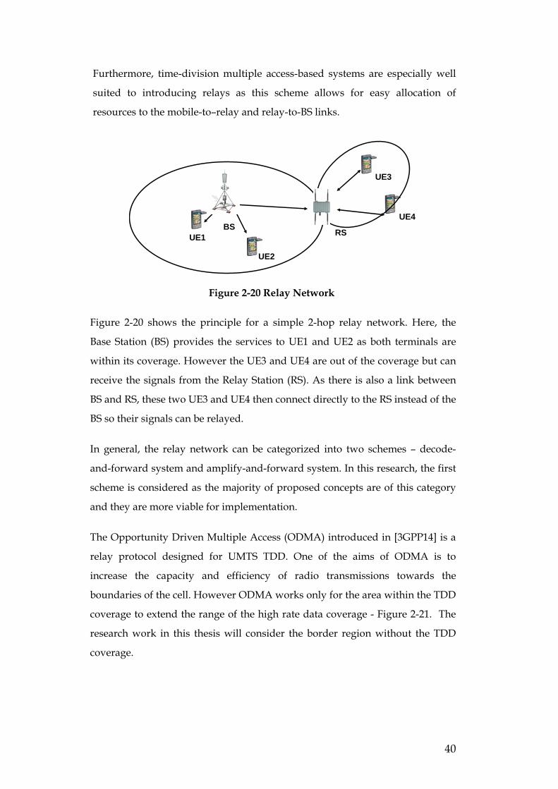
Figure 2-20 Relay Network
Figure 2-20 shows the principle for a simple 2-hop relay network. Here, the
Base Station (BS) provides the services to UE1 and UE2 as both terminals are
within its coverage. However the UE3 and UE4 are out of the coverage but can
receive the signals from the Relay Station (RS). As there is also a link between
BS and RS, these two UE3 and UE4 then connect directly to the RS instead of the
BS so their signals can be relayed.
In general, the relay network can be categorized into two schemes – decode-
and-forward system and amplify-and-forward system. In this research, the first
scheme is considered as the majority of proposed concepts are of this category
and they are more viable for implementation.
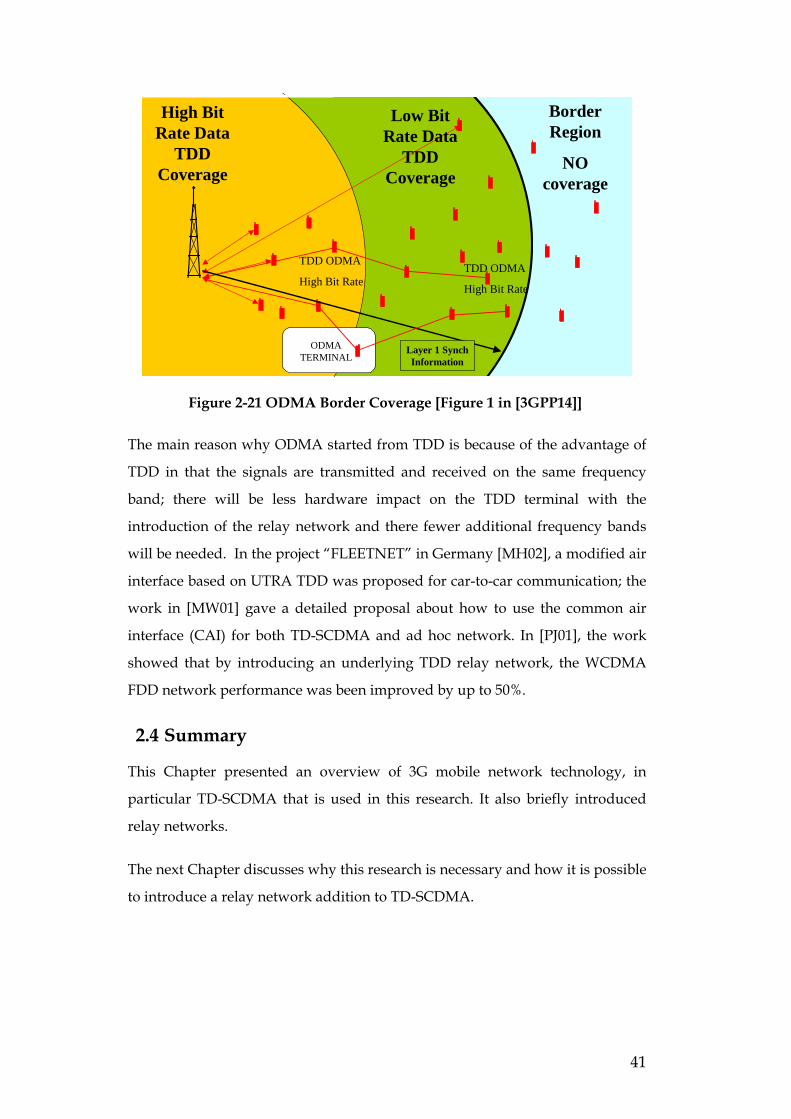
The Opportunity Driven Multiple Access (ODMA) introduced in [3GPP14] is a
relay protocol designed for UMTS TDD. One of the aims of ODMA is to
increase the capacity and efficiency of radio transmissions towards the
boundaries of the cell. However ODMA works only for the area within the TDD
coverage to extend the range of the high rate data coverage - Figure 2-21. The
research work in this thesis will consider the border region without the TDD
coverage.
41
ODMATERMINAL
High BitRate Data
TDDCoverage
Low BitRate Data
TDDCoverage
TDD ODMA
High Bit Rate
TDD ODMA
High Bit Rate
BorderRegion
NOcoverage
Layer 1 SynchInformation
Figure 2-21 ODMA Border Coverage [Figure 1 in [3GPP14]]
The main reason why ODMA started from TDD is because of the advantage of
TDD in that the signals are transmitted and received on the same frequency
band; there will be less hardware impact on the TDD terminal with the
introduction of the relay network and there fewer additional frequency bands
will be needed. In the project “FLEETNET” in Germany [MH02], a modified air
interface based on UTRA TDD was proposed for car-to-car communication; the
work in [MW01] gave a detailed proposal about how to use the common air
interface (CAI) for both TD-SCDMA and ad hoc network. In [PJ01], the work
showed that by introducing an underlying TDD relay network, the WCDMA
FDD network performance was been improved by up to 50%.
2.4 Summary
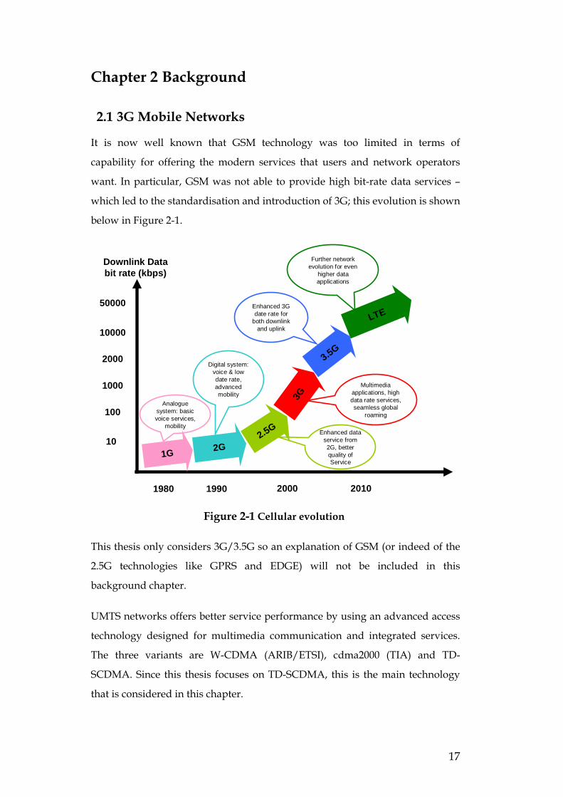
This Chapter presented an overview of 3G mobile network technology, in
particular TD-SCDMA that is used in this research. It also briefly introduced
relay networks.
The next Chapter discusses why this research is necessary and how it is possible
to introduce a relay network addition to TD-SCDMA.
42
Chapter 3 Interference within TD-SCDMA networks
3.1 Potential Problems within TD-SCDMA network
As one of the standard 3G radio access network techniques, currently TD-
SCDMA technology is being developed mainly in China. At the time of writing
this thesis, TD-SCDMA has been used in the 2008 Beijing Olympics to provide
voice and data applications. In October 2008, the Ministry of Industry and
Information Technology of China announced that the penetration of TD-
SCDMA subscribers in the 10 cities in China where it is available reached three
hundred thousand. Meanwhile, the next stage of the TD-SCDMA network
expansion is continuing as planned. According to the plan, there will be another
28 cities covered by TD-SCDMA. The overall amount of TD-SCDMA
subscribers has reached 2 million after 2008 Beijing Olympic and it optimized
estimation is till 2012, the total TD-SCDMA subscribers might be 50 million.
Although the launch of TD-SCDMA is in its initial phase across China, it is
expected to grow rapidly, as witnessed by the current heavy advertising. This
research is focussing on topics such as the network’s performance under heavy
traffic conditions in cities and in large rural areas. One particular area of
concern to network operators is what should be the proper cell radius for TD-
SCDMA networks under different conditions.
As with all CDMA technologies, interference is a key aspect when doing the
network planning as well as the propagation model; many interference factors
can influence the coverage.
For example, the multiple DwPCH signals from different cells within one
geographical area will cause inference. Two possible solutions for this are:
• the N-frequency technology addressed in the previous chapter;
• using “DwPTS blanking”.
DwPTS blanking means that the DwPCH signal of one cell is not continuously
transmitted, but uses a scheduling scheme to determine when the different
DwPCH signals from different cells should be transmitted to avoid interference
43
among them. Although that might introduce more difficulties for a mobile
terminal searching cells to determine which to camp to, it is possible, by using
repeated attempts, for the terminal to finally capture the best cell in its cell list.
[3GPP13]
Besides the downlink pilot interference, the uplink pilot interference is another
issue since all the terminals attempting to gain service are accessing the UpPCH.
If this UpPCH is interfered by other signals, the cell access success rate will
drop dramatically. This problem becomes more serious when adopting the N-
frequency technology because all the carriers within the cell share a single time
slot. In addition, downlink DwPCH signals from other cells can interfere with
the UpPCH signal because the extra propagation delay means they overspill
their time slot and if this overspill is greater than the guard period then
interference occurs – remembering that uplink and downlink channels are on
the same frequency.
One possible method to solve the problem of DwPCH / UpPCH inter-cell
interference is to allow the network to dynamically allocate the UpPCH in any
uplink time slot. Then, via broadcasting the allocation, all the terminals within
this area will adjust their sub frame structure accordingly.
At the edge of the cell, these problems will be more serious when there are
more users. This research will focus on solving the coverage problems at the
edge of the cell or the black hole in the network.
3.2 Coverage problems within TD-SCDMA network
As shown in Figure 3-1, the delay will be further at the edge of the cell. If the
terminal is near the cell edge, after receiving the signals from the network, it
will adjust its timing to advance the signals it transmits to make sure they arrive
at the NodeB simultaneously with those from other terminals all around the cell.
The further the terminal is away from the NodeB, the more it should advance
its signal timing. The following diagram shows the normal status of signalling
transmission and receiving between the NodeB and one terminal at the edge of
cell (the x axis is time):
44
UE TX
NB RX
DL DL
DL
DL DL
DL
DLDL
UL UL DL
Dw GP Up UL UL UL DL
GP Up
Dn Dw GP Up
UL
UL
UL UL DL
Dn Dw GP Up UL UL UL
NB TX
Dn
Dn
Dw
UE RX
DL
Timing Advance
Synchronized Signals received by NodeB
at site
at edge
at edge
at site
Figure 3-1 Cell Edge Normal Case
Dn: Downlink Timeslot 0, which is always configured as downlink, mainly to
do the cell broadcasting
Dw (DwPTS): downlink pilot time slot, for downlink synchronization
GP (Guard Period): main guard period for TDD operation,
Up (UpPTS): uplink pilot time slot, for uplink synchronization
UL: the Uplink Time Slot, while the TS1 is always allocated Uplink
DL: the Downlink Time Slot
NB TX: The Signals transmitted from the NodeB
UE RX: The signals received by the terminal
UE TX: The signals transmitted from the terminal
NB RX: The signals received by the NodeB
However, even with a carefully designed network, there are still more
possibilities to introduce interference in the network. The majority of
interference cases exist at the edge of the cell and two of the interference
scenarios are described below:
Scenario 1: If the terminal is at the edge of the cell, it might get
interference from the neighbouring cell. As shown in the following slot
diagram, the UE1 is within the NodeB1’s coverage and is receiving the
delayed signals from NodeB1. However, with the timing advance
scheme, UE1 can still camp on NodeB1, but, as NodeB 2 is NodeB1’s
45
neighbour and its downlink transmission is received by UE1 as well, but
with further delay due to the greater distance, the UE1 cannot identify
the cell information from the two intra- frequency downlink cell
broadcast time slot. This will directly influence the network access rate
and handover success rate. This situation did occur during the first pre-
commercial TD-SCDMA trial in China and caused significant
operational problems.
DL DL
DLUp
UL UL UL DL
DLUL UL DLUL
UL UL UL DL
DwDnNB2 TX
NB1 TX DL DLDn Dw GP Up
GP
UE1 RX Dn Dw GP Up
Repeat Cell Searching
At this time point, two downlink cell broadcast time slot are Intra-frequency interfered with each other the UE1 fails to identify the cell information
UE spends much more time for cell searching
frequently
at site
at site
at edge
Failed
Figure 3-2 Interference Scenario 1
NB1 TX: The Signals transmitted from the NodeB1
NB2 TX: The Signals transmitted from the NodeB2
UE1 RX: The signals received by the first terminal
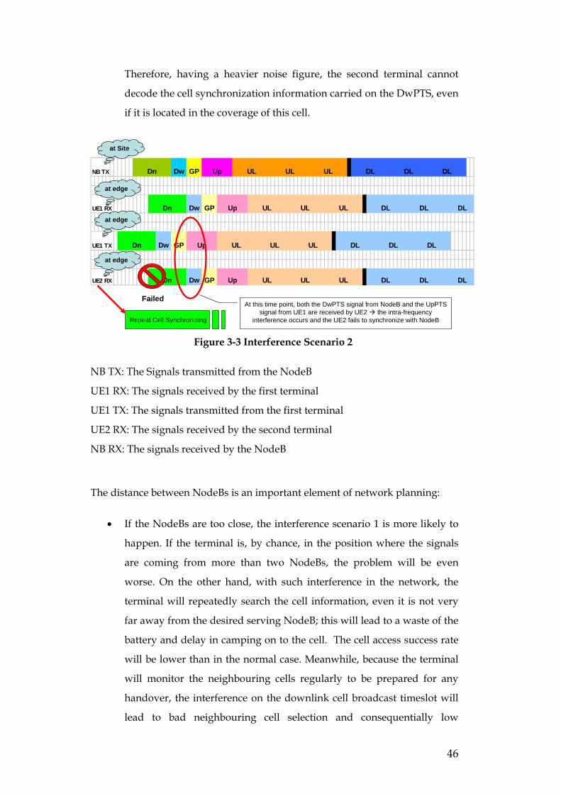
Scenario 2: There also exists another interference scenario, this time
with two users near to each other at the edge of the cell who will have
interference problems particularly when one is searching and the other
is sending: the terminal searching is looking for downlink synchronized
signalling but will also see the heavy intra-frequency interference from
another terminal sending on the uplink. The more terminals there are,
the heavier the interference will be.
As shown in the following slot diagram, the first terminal’s uplink pilot
signals interfere with the second terminal’s downlink pilot Pilot signals.
46
Therefore, having a heavier noise figure, the second terminal cannot
decode the cell synchronization information carried on the DwPTS, even
if it is located in the coverage of this cell.
NB TX
UE1 RX
UE1 TX
UE2 RX Dn
Dn
Dw GP
Dn
DLDn
GP Up
UL ULUp
Dw UL UL
UL
UL DL
Dw GP Up UL UL UL DL DL DL
DL
DL DL
DL
DLDw GP Up UL UL UL DL DL
Repeat Cell Synchronizing
At this time point, both the DwPTS signal from NodeB and the UpPTSsignal from UE1 are received by UE2 the intra-frequency
interference occurs and the UE2 fails to synchronize with NodeB
at Site
at edge
at edge
at edge
Failed
Figure 3-3 Interference Scenario 2
NB TX: The Signals transmitted from the NodeB
UE1 RX: The signals received by the first terminal
UE1 TX: The signals transmitted from the first terminal
UE2 RX: The signals received by the second terminal
NB RX: The signals received by the NodeB
The distance between NodeBs is an important element of network planning:
• If the NodeBs are too close, the interference scenario 1 is more likely to
happen. If the terminal is, by chance, in the position where the signals
are coming from more than two NodeBs, the problem will be even
worse. On the other hand, with such interference in the network, the
terminal will repeatedly search the cell information, even it is not very
far away from the desired serving NodeB; this will lead to a waste of the
battery and delay in camping on to the cell. The cell access success rate
will be lower than in the normal case. Meanwhile, because the terminal
will monitor the neighbouring cells regularly to be prepared for any
handover, the interference on the downlink cell broadcast timeslot will
lead to bad neighbouring cell selection and consequentially low
47
handover success rate. Remember that the small cell coverage will cause
frequent handover activities. The result is that there will be an adverse
impact on the network capacity as fewer users will be served by the
network. The above two aspects can lead to a lower network utility and
efficiency.
• If the distance between NodeBs is too far, the interference scenario 2
cannot be avoided. Although the site coverage is optimized compared to
the scenario 1, the interference problem still exists. Those terminals that
are interfered with by other neighbouring terminals’ uplink pilot signals
will experience difficulties in synchronizing with the cell. As stated
previously, the consequence will be a low access success rate and low
handover success rate. Furthermore, with the distance between the
NodeB and the terminals at the cell edge being relatively long, if the
handover attempts fail because of the bad synchronization, the
handover call drop rate will increase greatly. Besides the negative user
experience, those users will attempt to connect repeatedly and will also
interfere with other terminals. Similarly to the result of scenario 1, the
failure call attempts and handover attempts decrease the network
capacity.
From the above analysis, this research proposes a new network structure with the
intention of improving TD-SCDMA cell coverage suggestion and optimizing the
capacity of the TD-SCDMA network via lowering the interference at the cell edge.
3.3 Adding relay to N-frequency TD-SCDMA
If coverage is to be extended in a TD-SCDMA network then either more NodeBs
have to be added (which is costly) or the power has to be increased – which can
be self-defeating as it can increase the problem of interference.
By using the concept of relay networks, introduced in the previous chapter, the
flexibility that they offer can benefit the network a lot while extending the
coverage and enhancing the capacity.
48
BSUE
UE
RS
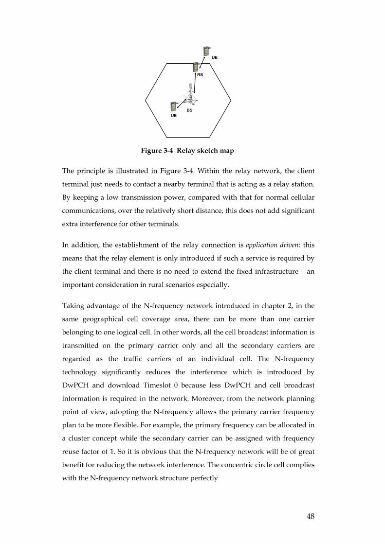
Figure 3-4 Relay sketch map
The principle is illustrated in Figure 3-4. Within the relay network, the client
terminal just needs to contact a nearby terminal that is acting as a relay station.
By keeping a low transmission power, compared with that for normal cellular
communications, over the relatively short distance, this does not add significant
extra interference for other terminals.
In addition, the establishment of the relay connection is application driven: this
means that the relay element is only introduced if such a service is required by
the client terminal and there is no need to extend the fixed infrastructure – an
important consideration in rural scenarios especially.
Taking advantage of the N-frequency network introduced in chapter 2, in the
same geographical cell coverage area, there can be more than one carrier
belonging to one logical cell. In other words, all the cell broadcast information is
transmitted on the primary carrier only and all the secondary carriers are
regarded as the traffic carriers of an individual cell. The N-frequency
technology significantly reduces the interference which is introduced by
DwPCH and download Timeslot 0 because less DwPCH and cell broadcast
information is required in the network. Moreover, from the network planning
point of view, adopting the N-frequency allows the primary carrier frequency
plan to be more flexible. For example, the primary frequency can be allocated in
a cluster concept while the secondary carrier can be assigned with frequency
reuse factor of 1. So it is obvious that the N-frequency network will be of great
benefit for reducing the network interference. The concentric circle cell complies
with the N-frequency network structure perfectly
49
• The transmission power of each carrier can be allocated according to the
needs; by adjusting the power value, the coverage of each carrier can be
different within the cell coverage. Basically, the transmitted power of the
primary carrier will guarantee covering the whole planned cell coverage
all the time (the so-called “outer loop circle”) while the secondary
carriers use less power to cover the inner loop circle.
• At the edge of each cell, only one carrier from an individual cell might
cause interference any other inner circle carriers will definitely have no
overlap with neighbouring cells’ inner circle carriers. Therefore the
interference at the cell edge will reduce to a certain extent.
This research, therefore, combines the N-frequency technology and the
concentric circle cell concept with relay network technology, applying the same
radio access technology –TD-SCDMA to all the air interfaces, to solve the
coverage problems at the edge of the cell or the “black holes” in TD-SCDMA
networks.
[HN01] investigated the work about introducing a relay network into a
WCDMA network. Similar to the proposal in this research, the air interface is
the same for both the WCDMA and relay networks. However as stated in
[HN01], TDD is more suitable for this relay combination as in a WCDMA FDD
system the terminal cannot transmit and receive signals on the same frequency
band, which makes the radio more complicated for relaying.
When importing another network into the TD-SCDMA network, the most
important issue is to avoid introducing more interference. The N-frequency and
concentric circle cell make the TD-SCDMA network more suitable for
combining with relay network where the hybrid network structure will extend
the coverage and reduce the interference greatly. The main advantage is that the
terminal acting as a relay station in the relay network will be covered only by
the cell primary carrier, so this terminal can take any of the secondary carriers
of the cell as the working frequency between itself and the client terminal. This
selected frequency has no intra-frequency interference with the primary carrier
in TD-SCDMA network.
50
This approach extends the coverage, therefore, without adding extra
interference.
Adding a relay network into a conventional cellular network has attracted quite
a lot of research interest. Most of the work related to TD-SCDMA has focused
on developing a suitable protocol for the integrated TD-SCDMA relay network.
[LX01] presents the appropriate TD-SCDMA air interface modification to
include ad hoc operations without changing the TD-SCDMA frame structure.
Corresponding radio resource management schemes are provided to ensure the
new air interface will apply to the hybrid system. Based on the work that
brought out one common air interface for both TD-SCDMA and relay network
parts [MW01], researchers from the same “National Mobile Communications
Research Laboratory, Southeast University” investigated the modification on
the MAC layer protocol to utilize the channel allocation efficiency in the TD-
SCDMA relay network [SZ01].
As stated in previous sections, this work is different, focusing on the
performance analysis of the TD-SCDMA relay network under the combination
of N-frequency and concentric circle cell concepts, which has not yet been
considered by any other work.
3.4 Approach
A normal ad hoc relay network structure will dynamically construct and de-
construct itself with the activities of the terminals comprising that network,
including as they move location. However, when considering the hybrid
TD-SCDMA relay network, a frequently changing network structure will cause
severe problems, with large increases in signalling traffic and non-guarantee in
service quality. Therefore, in this research, the approach taken stabilises the
hybrid network structure as much as possible.
The outline of the approach is:
• User terminals will act as the relay stations in the relay network to
provide access services to other users who are out of the TD-SCDMA
network’s coverage. Since this will benefit the network operator, at least
from the coverage point of view, the operator should set up promotional
51
schemes to encourage the users to work as the relay station in the relay
network, such as free traffic rewards or free application rewards.
Promotional schemes have been successfully used before in the mobile
industry, such as that currently adopted in China which is used to
encourage the “friendly users” in the TD-SCDMA pilot network. Within
2 months, there were more than 20,000 users using the TD-SCDMA
network in 5 cities. By using such schemes in the hybrid TD-SCDMA
relay network, the network operator can maximise the probability of
there being sufficient relay stations within the coverage area to provide
an adequate quality of service to those outside. Of course, a scheme
could exist where all users could act as relay stations whether they
wanted to or not, but in a competitive environment this might not be
good marketing, It should also be noted that acting as a relay station will
impact adversely on battery life as it will be transmitting even when the
subscriber is not using it, so the user should have some incentive.
• In order to avoid the relay network structure changing frequently
(called “floating” here), the TD-SCDMA network must have a strategy
for establishing the relay network and monitoring its performance. In
this research the approach is:
o It will always be the terminal that initiates the move to act as the
relay station in the relay network. If the terminal is in idle mode,
the user can manually send the “act as relay station request” to
the TD-SCDMA network in order to claim rewards.
o When the TD-SCDMA network receives the request, the network
will evaluate the terminal’s “credit” (such as current location,
recent movement statistics, previous service quality, application
capability) – the criteria for choice of relay station will be set by
the operator depending on its business plan. As this research
focuses on the coverage and interference influence of the hybrid
TD-SCDMA relay network, the criteria choices will not be
discussed further.
52
o If the request meets the criteria, the TD-SCDMA network will
send a response to the terminal together with necessary
parameters (such as which secondary frequency of the serving
TD-SCDMA cell the terminal should use as a relay station for
broadcast and what kind of packet data services that can be
forwarded by the terminal).
o When the response is received successfully by the terminal, it
will adjust its transmitter and receiver accordingly and start
working as a relay station in the relay network.
• Both the terminal and the TD-SCDMA network can terminate the relay
network based on certain rules. For example, if the TD-SCDMA network
discovers that the terminal acting as a relay station is active with its own
communication it will terminate the relay station role since continuation
of relay services will interfere with the TD-SCDMA network. Another
case is where the user wants to stop acting as a relay station, or the
terminal realises that the relay station role will adversely affect its own
performance, a message can be sent to the TD-SCDMA network to
terminate the role.
How this will work in different scenarios is discussed in the next section.
3.5 Research Scenarios
In GSM networks, the main type of service carried was voice, but after the
evolution to 2.5G or 2.75G, with GPRS and then EDGE, both voice and data
application are common and the trend is that data services are getting more and
more important. In this research, only packet data services are considered. The
reasons are:
• Normally uses who are running data application on their terminals are
not moving as frequently or as fast as voice users. This lower mobility
makes them a more suitable candidate for constructing a relay network;
this applies to both acting relay station and client terminals.
• The quality requirements for data services are generally not so stringent
as those for voice; users can bear more delay or jitter in the application.
53
This aspect is very important for the relay network which needs the
users to be more tolerant about the quality.
• The duration of a typical data application connection is much longer
than a voice application, which will introduce less signalling traffic in
the TD-SCDMA relay network.
Furthermore, according to [3GPP08], each TD-SCDMA carrier can serve only
one 384kbit/s user or three 128kbit/s users, which will not be the majority
business model in the real network. The reason for this is the scrambling code
limitation in TD-SCDMA. At the initial stage of constructing a new network, the
main intention of the operator is to attract as many users as possible to utilise
the network investment. So in this research, the non-HSDPA service model is
assumed to be packet switched 64kbit/s, which is the most likely wide used
packet date-rate. Meanwhile, HSDPA, which further optimises the network
resource usage via adopting the shared channel among all severing users, is
analyzed as well for further comparison between these two packet data service
technologies. The HSDPA user in this work is configured with peak data rate
384kbit/s and mean date rate 64kbit/s.
The normal objective for the cellular mobile network structure is consistent
coverage to provide seamless services; basically each cell will be surrounded by
six neighbouring cells and between them the handover management is
implemented.
Cell 1Cell 1
Cell 7Cell 7
Cell 5Cell 5
Cell 2Cell 2
Cell 3Cell 3
Cell 4Cell 4Cell 6Cell 6
Figure 3-5 Cellular Mobile Network
54
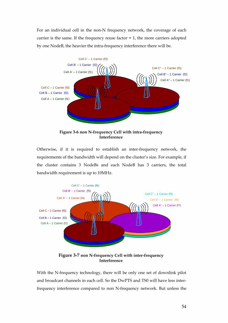
For an individual cell in the non-N frequency network, the coverage of each
carrier is the same. If the frequency reuse factor = 1, the more carriers adopted
by one NodeB, the heavier the intra-frequency interference there will be.
Cell A – 1 Carrier (f1)
Cell B – 1 Carrier (f2)
Cell C – 1 Carrier (f3)
Cell A’ – 1 Carrier (f1)
Cell B’ – 1 Carrier (f2)
Cell C’ – 1 Carrier (f3)
Cell A” – 1 Carrier (f1)
Cell B” – 1 Carrier (f2)
Cell C” – 1 Carrier (f3)
Figure 3-6 non N-frequency Cell with intra-frequency Interference
Otherwise, if it is required to establish an inter-frequency network, the
requirements of the bandwidth will depend on the cluster’s size. For example, if
the cluster contains 3 NodeBs and each NodeB has 3 carriers, the total
bandwidth requirement is up to 10MHz.
Cell A – 1 Carrier (f1)
Cell B – 1 Carrier (f2)
Cell C – 1 Carrier (f3)
Cell A’ – 1 Carrier (f4)
Cell B’ – 1 Carrier (f5)
Cell C’ – 1 Carrier (f6)
Cell A” – 1 Carrier (f7)
Cell B” – 1 Carrier (f8)
Cell C” – 1 Carrier (f9)
Figure 3-7 non N-frequency Cell with inter-frequency Interference
With the N-frequency technology, there will be only one set of downlink pilot
and broadcast channels in each cell. So the DwPTS and TS0 will have less inter-
frequency interference compared to non N-frequency network. But unless the
55
primary carrier’s frequency of each cell is allocated differently, the intra-
frequency interference can not be avoided.
Cell A – 3 Carriers (f1,f2,f3)
Cell B – 3 Carriers (f1,f2,f3) Cell C – 3 Carriers (f1,f2,f3)
Figure 3-8 N-frequency Cell with intra-frequency interference
Dense urban and rural areas are selected in this research as the two coverage
objects for analysis.
Most big cities, such as Beijing and Shang Hai have heavy mobile traffic due to
the large population and high usage profiles. The bottleneck in network
establishment is not the coverage but the capacity in dense urban areas. In
another words, the distance between two sites in big cities is very close in order
to make sure there is enough network resource to serve the heavy network load.
In such circumstances, the interference scenario 1, mentioned in the previous
section will occur.
On the contrary, in rural areas, such as in the country side or at the seaside, the
traffic is light but the area is huge. So the bottleneck in the rural area is the
coverage. The operator prefers the smallest number sites for the maximum
coverage. Thus, interference scenario 2 will happen.
In this research, the concentric circle cell is proposed to be used into the N-
frequency network with the aim of optimizing the frequency efficiency. One
solution is that apart from the primary carrier, which uses a different frequency
for every cell within a cluster, the first secondary carrier of each cell can use the
same frequency and the second secondary carrier can adopt another frequency,
including the same as the primary in another cell. So within a 5MHz allocation,
the frequency reuse factor is between 1 and 3, yet there is no heavy intra-
frequency interference on DwPTS and TS0 channels.
56
Cell B – 3 Carriers (f2,f1,f3)
Outer Circle-Primary Carrier (f2)
Inner Circle-Secondary Carrier (f1,f3)
Cell C – 3 Carriers (f3,f1,f2)Outer Circle-Primary Carrier (f3)
Inner Circle-Secondary Carrier (f1,f2)
Cell A – 3 Carriers (f1,f2,f3)
Outer Circle-Primary Carrier (f1)
Inner Circle-Secondary Carrier (f2,f3)
Figure 3-9 Concentric Circle Cell with Inter-frequency Interference
However, with the most frequency efficient scheme where the frequency reuse
factor is 1, the intra-frequency interference will still exist in the overlapping
areas.
Cell B – 2 Carriers (f1,f2,f3)
Outer Circle-Primary Carrier (f1)
Inner Circle-Secondary Carrier (f2,f3)
Cell C – 2 Carriers (f1,f2,f3)
Outer Circle-Primary Carrier (f1)
Inner Circle-Secondary Carrier (f2,f3)
Cell A – 2 Carriers (f1,f2,f3)Outer Circle-Primary Carrier (f1)
Inner Circle-Secondary Carrier (f2,f3)
Figure 3-10 Concentric Circle Cell with Intra-frequency Interference
The central shaded areas of each cell in Figure 3-10 above are covered by the
primary carrier and secondary carriers while the area beyond that is covered by
the primary carrier only. It is obvious from Figure 3-10 that at the edge of each
cell there are overlapping areas for the primary frequency, so that intra-
frequency interference cannot be totally avoided. Therefore, the relay network
is implemented here.
57
Cell B Cell B –– 3 Carriers 3 Carriers ((f1f1,f2,f3),f2,f3)
Cell A Cell A –– 3 Carriers 3 Carriers ((f1f1,f2,f3),f2,f3)
Cell C Cell C –– 3 Carriers 3 Carriers ((f1f1,f2,f3),f2,f3)
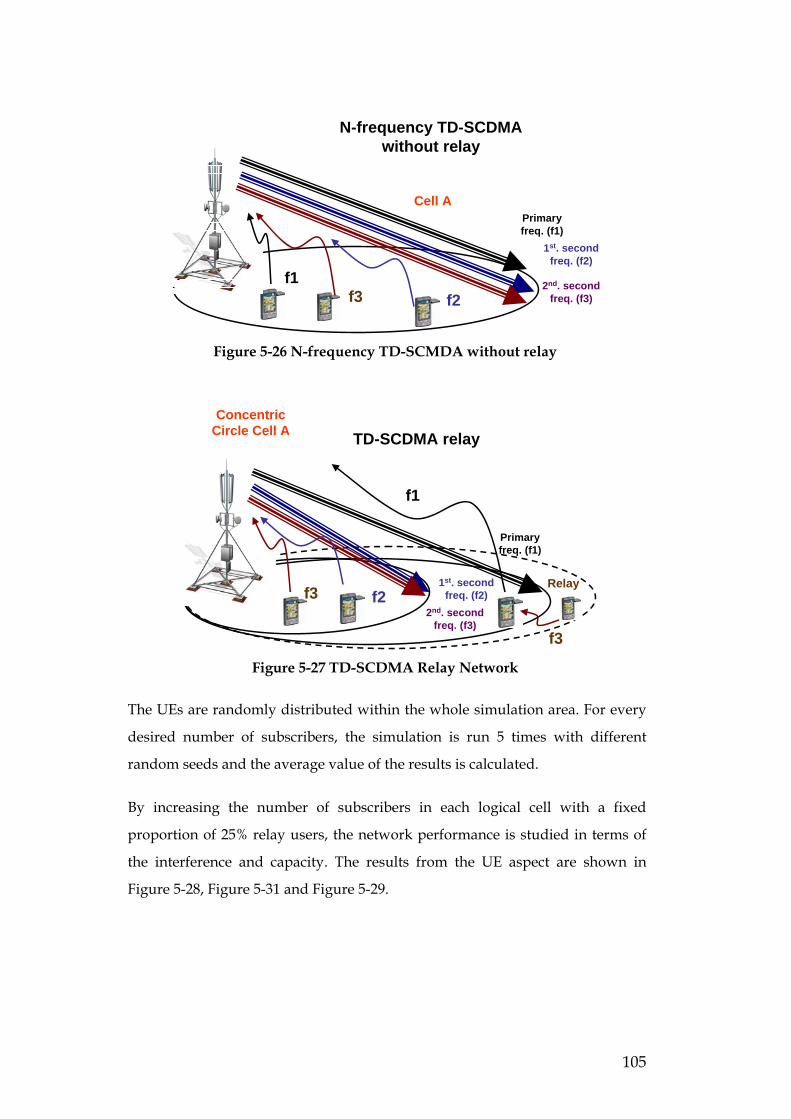
Figure 3-11 Hybrid TD-SCDMA relay Network
In Figure 3-11, the shaded area within the inner solid line is covered by the
primary carrier and secondary carriers while the area between the inner and
outer solid lines is covered by the primary carrier only. The area between the
outer solid line and the dashed line is the area covered by the relay network,
which can take any of the inner circle’s frequencies as the working frequency.
The ideal relay TD-SCDMA network structure is that there will be no coverage
overlap of the TD-SCDMA N-frequency network while the gap areas are served
by the relay network.
The radio access technology for the relay network segment is proposed to be
TD-SCDMA [LX01]-[DS01]. The reasons are:
• The terminals within the TD-SCDMA and relay network only have to
support one kind of access technology which is the simplest way to
develop the product.
• The same frame structure can shorten the translation processing time in
the relay station acting terminal node.
• Applications from the terminal acting as a relay station and client
terminal combination are easier to implement because the same air
interface is used.
58
• Similar algorithms, such as power control, synchronization scheme and
radio resource management, can be implemented in both the TD-
SCDMA network and relay network, which is utilising the software
development.
This research will consider two aspects of this TD-SCDMA relay network.
• One aspect is the suitable cell radius of the TD-SCDMA network and the
proper coverage of relay network, for both dense urban areas and rural
areas, As mentioned in section 3.2, the individual NodeB will cover a
large area in rural communities.; in the big cities, because of the thick
buildings, “black holes” normally exists, especially at the corner of
buildings. This research will, therefore, verify to what extend the relay
network can enlarge the TD-SCDMA network’s coverage in rural areas
or whether the relay network can help avoid “black holes” in dense
urban areas.
• The other aspect is to analyze the influence of the TD-SCDMA/relay
combination on interference and capacity. As mentioned in section 1.2,
two different scenarios in different types of area that bring out different
aspects are considered for the interference and capacity analysis in this
research:
o HSDPA data service in dense urban
o Non-HSDPA data service in rural
Both have the same rationale: the adoption of the concentric circle cell in the hybrid
network structure will dramatically minimize the intra-frequency interference in TD-
SCDMA networks with the aim of increasing the capacity and coverage of the hybrid
network than the non-concentric circle cell configuration.
These are considered below.
HSDPA service in dense urban areas
• The primary frequency is used by the network to broadcast to all the
terminals in the outer circle cell areas while secondary frequencies serve
the inner circle cell.
59
• One of the secondary frequencies is used by the relay station in the relay
network to broadcast to all the terminals positioned in the relay network
only.
• Because in multi-carrier HSDPA applications, the downlink traffic
transmission channels are shared by HSDPA users, and neither the relay
station acting terminal nor the client acting terminal will occupy the
network resource continually.
• Under the multi-carrier HSDPA structure, each NodeB supports more
than one carrier but the terminal in this research supports only one
carrier at a time, which reflects the situation of the current TD-SCDMA
terminals as it is the most cost effective solution for the terminal vendors
and the end users.
Non-HSDPA data service in rural areas
o The primary frequency is used by the network to broadcast to all the
terminals in the outer circle cell areas while secondary frequencies serve
the inner circle cell(s).
o One of the secondary frequencies is used by the relay station in the relay
network to broadcast to all the terminals positioned in the relay area
only.
o The relay station will receive and send the client’s data to the TD-
SCDMA network via the primary carrier in one frame and communicate
with the client via the secondary carrier in the following frame with the
continuous resource allocation within a packet call.
3.6 Summary
This chapter showed how the TD-SCDMA network could in principle be
extended by a relay segment in order to address some of the problems such as
interference limiting the coverage and capacity of a conventional network. This
is a new concept for TD-SCDMA networks,
60
In the next chapter, the link budget of the TD-SCDMA network and relay
network will be calculated and using that result, the cell coverage of this hybrid
TD-SCDMA relay network will be determined. The simulation method for
capacity and interference will then be introduced in the subsequent chapter
together with the simulation results.
61
Chapter 4 Link Budget
4.1 Introduction
In this section, the link budgets for the TD-SCDMA network and the relay
network are calculated. This is necessary in order to calculate the coverage area
of the combined hybrid network and the work on extending this link budget to
the hybrid segment is new.
In a TD-SCDMA network, both the control channel and the traffic channel
should be taken into account when considering the network planning and cell
coverage. In the product realization from industry, the power of NodeB
downlink control and traffic channel are treated differently while the terminal
uplink control and traffic channel are treated similarly
Considering these in turn:
NodeB downlink control and traffic channel
• The NodeB will always transmit the control signals, especially the cell
broadcast signals, with maximum power without any power control.
This is unlike the traffic channel where power control is used to lower
the interference within the network.
• The total transmission power of each timeslot is set by the NodeB’s
power amplifier and all the timeslots have the same signal power before
being sent to the antenna.
• Furthermore the antenna will treat all the timeslots the same. As all the
cell broadcast channels are allocated in TS0 only and no traffic channel
will be allocated in TS0, the TS0 power will be fully used by the cell
broadcast signals. On the other hand, as TD-SCDMA inherits the code
division multiple accesses from CDMA system, the more terminals that
camp onto a certain timeslot, the lower the downlink transmission
power that will be seen from the NodeB by each terminal since CDMA is
used within the timeslot. Also, in order to make sure all the terminals on
62
the same timeslot can be served properly, the NodeB will use the
transmission power relevant to the service type in use.
• The major difference between the downlink control channel and the
traffic channel is that there is 8dB smart antenna beam forming gain on
the traffic channel but not on control channel. The reason is that the
control channel has to cover the whole cell areas so there can be no
directed beam on the control channel.
So from the downlink point of view, the power in the control channel will always be
lower that that in the traffic channel.
Uplink Control and traffic Channel
• The UpPCH is a solo timeslot in the TD-SCDMA frame structure so
there is no transmission power limitation on it. A multi-access attempt
scheme is implemented here to ensure the terminal can continually
synchronize with the network if conflicts occur due to too many
attempts.
• The uplink access channel can be allocated to any of the uplink timeslot
which normally occupies 2 codes. The rest of the codes are used as
uplink traffic channel. So the uplink control channel and traffic channel
will share the total transmission power within each timeslot
• On the Uplink, the smart antenna diversity and joint detection are
performed both for uplink access channel and traffic channel
Based on the above information, in this research only the uplink traffic channel
and downlink control channel are considered for the uplink and downlink link
budget calculation.
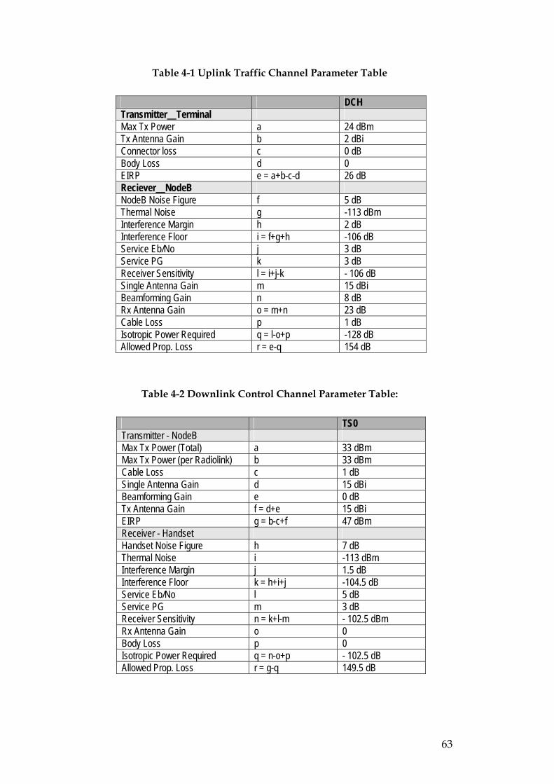
4.2 Traffic Channel Parameters
The values from these tables have been taken from [HX01][WQ01], [3GPP04]
and [3GPP05],
63
Table 4-1 Uplink Traffic Channel Parameter Table
DCH Transmitter__Terminal Max Tx Power a 24 dBm Tx Antenna Gain b 2 dBi Connector loss c 0 dB Body Loss d 0 EIRP e = a+b-c-d 26 dB Reciever__NodeB NodeB Noise Figure f 5 dB Thermal Noise g -113 dBm Interference Margin h 2 dB Interference Floor i = f+g+h -106 dB Service Eb/No j 3 dB Service PG k 3 dB Receiver Sensitivity l = i+j-k - 106 dB Single Antenna Gain m 15 dBi Beamforming Gain n 8 dB Rx Antenna Gain o = m+n 23 dB Cable Loss p 1 dB Isotropic Power Required q = l-o+p -128 dB Allowed Prop. Loss r = e-q 154 dB
Table 4-2 Downlink Control Channel Parameter Table:
TS0 Transmitter - NodeB Max Tx Power (Total) a 33 dBm Max Tx Power (per Radiolink) b 33 dBm Cable Loss c 1 dB Single Antenna Gain d 15 dBi Beamforming Gain e 0 dB Tx Antenna Gain f = d+e 15 dBi EIRP g = b-c+f 47 dBm Receiver - Handset Handset Noise Figure h 7 dB Thermal Noise i -113 dBm Interference Margin j 1.5 dB Interference Floor k = h+i+j -104.5 dB Service Eb/No l 5 dB Service PG m 3 dB Receiver Sensitivity n = k+l-m - 102.5 dBm Rx Antenna Gain o 0 Body Loss p 0 Isotropic Power Required q = n-o+p - 102.5 dB Allowed Prop. Loss r = g-q 149.5 dB
64
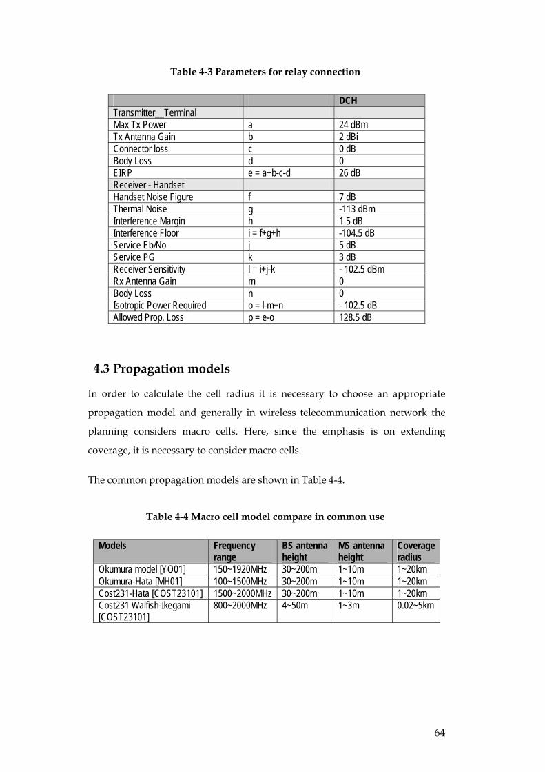
Table 4-3 Parameters for relay connection
DCH Transmitter__Terminal Max Tx Power a 24 dBm Tx Antenna Gain b 2 dBi Connector loss c 0 dB Body Loss d 0 EIRP e = a+b-c-d 26 dB Receiver - Handset Handset Noise Figure f 7 dB Thermal Noise g -113 dBm Interference Margin h 1.5 dB Interference Floor i = f+g+h -104.5 dB Service Eb/No j 5 dB Service PG k 3 dB Receiver Sensitivity l = i+j-k - 102.5 dBm Rx Antenna Gain m 0 Body Loss n 0 Isotropic Power Required o = l-m+n - 102.5 dB Allowed Prop. Loss p = e-o 128.5 dB
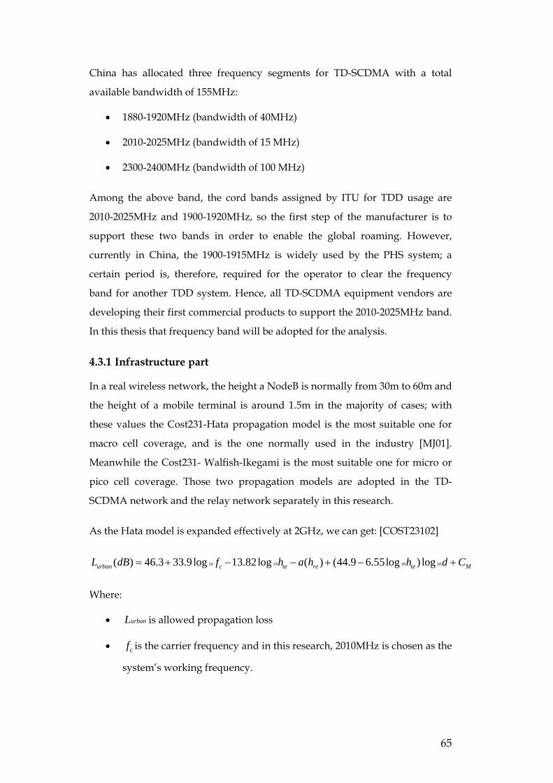
4.3 Propagation models
In order to calculate the cell radius it is necessary to choose an appropriate
propagation model and generally in wireless telecommunication network the
planning considers macro cells. Here, since the emphasis is on extending
coverage, it is necessary to consider macro cells.
The common propagation models are shown in Table 4-4.
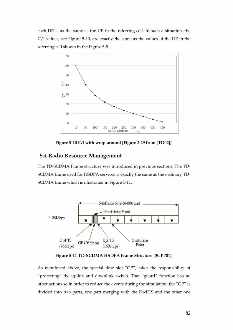
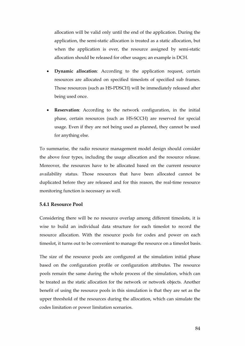
As mentioned above, the special time slot “GP”, takes the responsibility of
“protecting” the uplink and downlink switch. That “guard” function has no
other actions so in order to reduce the events during the simulation, the “GP” is
divided into two parts, one part merging with the DwPTS and the other one
0
10
20
30
40
50
60
70
10 50 100 150 200 250 300 350 400 450距离小区中心距离 (m)
信噪
比 (dB)
C/I
BS-UE Distance
0
10
20
30
40
50
60
70
10 50 100 150 200 250 300 350 400 450距离小区中心距离 (m)
信噪
比 (dB)
C/I
BS-UE Distance
83
merging with the UpPTS. Therefore, the simplified TD-SCDMA HSDPA frame
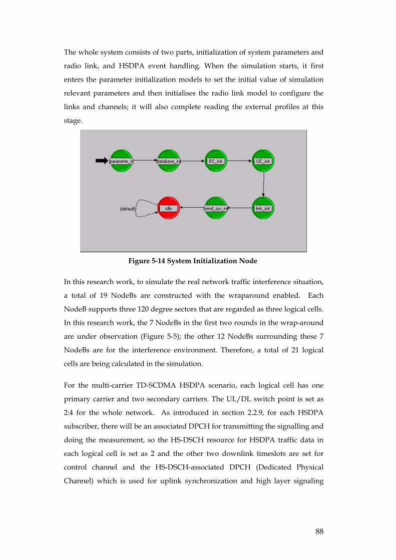
structure used in this simulation platform is shown in Figure 5-12.
TS0 TS1 TS2 TS3 TS4 TS5 TS6
DwPTS UpPTS Figure 5-12 TD-SCDMA Frame Structure in Simulation Platform
The radio resource is the valuable resource in the wireless communication
networks and so is one of the most important operational objects in the system
simulation. For TD-SCDMA system, the radio resource includes the frequencies,
the time slots, the codes and the power. After introducing the smart antenna
techniques, the space resource is treated as another dimension of radio resource.
However, the utility of space resource depends on the specific antenna
technologies used, unlike the codes or power that have theoretical limits. So in
the current simulation platform, only the frequencies, time slots, codes and
power are regarded as the core radio resource to be considered in the research.
The basic operations for resources consist of: resource allocating, resource
releasing and resource usage observing.
Resource allocation
Generally the resource allocation methods include:
• Static allocation: According to the network configuration, in the
network initial phase, this approach allocates the corresponding
resource. This allocation will take effect during the whole lifecycle of
simulation and cannot be used by others. Because the sub-frame of TD-
SCDMA system has periodicity, the static allocation resource will
periodically occupy the same assigned resource in every sub-frame and
there will be no changes of the location within the timeslots. During the
whole simulation process, the static resource allocation does not need to
be released at all, resources such as P-CCPCH.
• Semi-static allocation: According to the network configuration, the
radio resource is dynamically allocated for certain usage and this
84
allocation will be valid only until the end of the application. During the
application, the semi-static allocation is treated as a static allocation, but
when the application is over, the resource assigned by semi-static
allocation should be released for other usages; an example is DCH.
• Dynamic allocation: According to the application request, certain
resources are allocated on specified timeslots of specified sub frames.
Those resources (such as HS-PDSCH) will be immediately released after
being used once.
• Reservation: According to the network configuration, in the initial
phase, certain resources (such as HS-SCCH) are reserved for special
usage. Even if they are not being used as planned, they cannot be used
for anything else.
To summarise, the radio resource management model design should consider
the above four types, including the usage allocation and the resource release.
Moreover, the resources have to be allocated based on the current resource
availability status. Those resources that have been allocated cannot be
duplicated before they are released and for this reason, the real-time resource
monitoring function is necessary as well.
5.4.1 Resource Pool
Considering there will be no resource overlap among different timeslots, it is
wise to build an individual data structure for each timeslot to record the
resource allocation. With the resource pools for codes and power on each
timeslot, it turns out to be convenient to manage the resource on a timeslot basis.
The size of the resource pools are configured at the simulation initial phase
based on the configuration profile or configuration attributes. The resource
pools remain the same during the whole process of the simulation, which can
be treated as the static allocation for the network or network objects. Another
benefit of using the resource pools in this simulation is that they are set as the
upper threshold of the resources during the allocation, which can simulate the
codes limitation or power limitation scenarios.
85
5.4.2 Codes Resource Pool
Regarding the codes within the TD-SCDMA HSDPA cell, they are shared
resource, no matter whether uplink or downlink: so the usage allocation of the
codes is within the scope of the cell. As each cell will map to a solo NodeB in
this simulation platform, the codes resource pool of the cell can be designed as
one of the NodeB’s attributes. The uplink/downlink switch point will affect the
total amount of codes for uplink and downlink. Furthermore, the codes for HS-
PDSCH are independent from other physical layer channels, these two resource
categories have to be separated. There is an explicit definition for the codes of
HS-PDSCH.
On each timeslot, the parameters link_direction, HSDPA_code_num and
nonHSDPA_code_num will be configured according to the cell profile in the
simulation initial phase. As stressed in the background chapter, the
uplink/downlink switch point for the whole network should be set the same to
avoid uplink/downlink overlap interference (if certain protection mechanisms
are executed, the interference influence might be optimized – but this is not the
focus in this research work so there will be no more discussion on this item), so
the link_direction for all the cells should be the same. However, the
configuration of HSDPA_code_num and nonHSDPA_code_num can be
different to simulate the co-existence of HSDPA cell and non-HSDPA cell. Note
that the HSDPA_code_num here only covers the codes for downlink HS-
PDSCH, not including the codes for HS-SCCH or DPCH. It neither covers the
downlink non-HSDPA DCH. The HSDPA_code_num is always set as 0 for TS0
(which is not used for HS-PDSCH defined in the standard), uplink timeslots
and TD-SCDMA special timeslots.
5.4.3 Power Resource Pool
Within each timeslot, the NodeB power resources are shared by multiple UEs’
multiple channels. Meanwhile the total power for HS-PDSCH is separated from
the total power for other physical layer channels. The usage of these two
categories is independent.
Within each timeslot, the UE power resources are shared by multiple channels.
86
In the simulation platform, the power resource pools are created separately for
NodeB and UE. For NodeB, the downlink HSDPA_power means the total
power for HS-PDSCH; in the uplink the HSDPA_power and the non-
HSDPA_power are always 0.
For a UE that is not acting as the relay station, there is no need to configure the
HSDPA power for the uplink so the HSDPA_power for uplink timeslots is
always 0. But the non-HSDPA_power is decided by the UE’s capability and
both the downlink HSDPA_power and non-HSDPA_power are always 0 for the
UE.
For the UE acting as a relay station, there will be two sets of resource allocation:
one follows the rule for the NodeB’s (communicating with a relayed UE) and
the other follows the UE rule (communicating with the NodeB). The system will
call the corresponding configuration based on the role during the packet call.
5.4.4 Resource allocation list
The resource allocation status has to be recorded all the time. The remaining
resources can be determined after subtracting the already allocated resources,
so the upper limit can calculated for further resource allocation. Based on the
current allocation of resources allocation, the simulation system can use the
corresponding codes and power to transmit the signals.
The four different resources allocation methods mentioned above bring more
complexity to the modulation in the simulation platform. For example, the
resources might not only be used in the current sub frame, but also the
following sub frames. Besides, the occupation on the following sub frames
might be permanent (static allocation), or be valid for certain period (semi-static
allocation), or just be valid once (dynamic allocation). Therefore the data
structure should not only record the resource usage of the current sub frame
but the following sub frames. Additionally it needs to have the capability of
recording the different resource allocation methods and keep updating the data
when the resource allocation status changes. Because the period of static
allocation and semi-allocation occur on every timeslot, an individual resource
allocation list is designed for every timeslot.
87
To realize that requirement, the “List” type of OPNET is used here. One of the
advantages of using “List” here is that the resource record number for every
timeslot can be different. Furthermore, it is easy to carry out the operations on
adding or deleting the resource allocation to reflect the updates of the resource
allocation.
5.4.5 General Process
Figure 5-13 gives the overall view of the simulation flow chart. The external
interface allows the user to set common parameters for the simulation scenarios,
such as AMC, HARQ and scheduling schemes. Meanwhile the NodeB
configuration, smart antenna configuration and HSDPA resource configuration
are defined in the profile as well.
Start
User Interface Parameters Initialization
Environment Parameters Initialization
Traffic Distribution Parameters Initialization
Traffic Distribution Parameters Initialization
Simulation Environment Setup
Param
eter Initialization Phase
Antenna Gain Initialization
Radio Link Initialization & Setup
Slow Fading Initialization & Setup
Fast Fading Initialization & Setup
Timing initialization
Radio Link Initialization P
hase
Traffic Flow Initialization & Generation
Simulation Timing-Driven Control
End
HSD
PA Event H
andel Module
RNC Initialization & Setup
Node B Initialization & Setup
UE Initialization & Setup
Figure 5-13 Simulation Platform Flow Chart [Fig2 from [DJ01]]
88
The whole system consists of two parts, initialization of system parameters and
radio link, and HSDPA event handling. When the simulation starts, it first
enters the parameter initialization models to set the initial value of simulation
relevant parameters and then initialises the radio link model to configure the
links and channels; it will also complete reading the external profiles at this
stage.
Figure 5-14 System Initialization Node
In this research work, to simulate the real network traffic interference situation,
a total of 19 NodeBs are constructed with the wraparound enabled. Each
NodeB supports three 120 degree sectors that are regarded as three logical cells.
In this research work, the 7 NodeBs in the first two rounds in the wrap-around
are under observation (Figure 5-5); the other 12 NodeBs surrounding these 7
NodeBs are for the interference environment. Therefore, a total of 21 logical
cells are being calculated in the simulation.
For the multi-carrier TD-SCDMA HSDPA scenario, each logical cell has one
primary carrier and two secondary carriers. The UL/DL switch point is set as
2:4 for the whole network. As introduced in section 2.2.9, for each HSDPA
subscriber, there will be an associated DPCH for transmitting the signalling and
doing the measurement, so the HS-DSCH resource for HSDPA traffic data in
each logical cell is set as 2 and the other two downlink timeslots are set for
control channel and the HS-DSCH-associated DPCH (Dedicated Physical
Channel) which is used for uplink synchronization and high layer signaling
89
transmission purpose. The HSDPA related uplink and downlink signalling
channel HS-SICH and HS-SCCH are configured as 4 for each logical cell.
When all the initialization work is done, the whole simulation will enter the
global timing initial stage. In this phase, the timing-control logical model
(Global Timer) will send the global timer signalling to the three main nodes:
RNC, NodeB, UE and the traffic generation model.
Figure 5-15 Global Timer Node
This interrupt will trigger those modules to do parameter initialization.
Afterwards, they will enter the “wait” state until another interrupt from an
inner node or outer node to trigger the new operation. Thereafter, the event-
driving mechanism will keep driving the progress of the simulation until the
end of the simulation time.
90
5.4.6 HSDPA Event Handling Process
ServiceService
NoNode Bde B
UE UE
MAC-hs buffer
HARQ
Simulation output
MAC-hs buffer
MAC-hs buffer
Flow control
Flow control
Flow control
RNC RNC
Flow control
Flow control
Flow control
RLC buffer
RLC buffer
RLC buffer
Traffic source
Traffic source
Traffic source
IubIubChannel 1Channel 2Channel ..Channel n
P-CCPCHHS-PDSCH
HS-SCCHHS-SICH
HARQChannel 1Channel 2Channel ..Channel n
AMCvideo streaming
WWW
FTP
Note:Note:
HO
Physical channel
Smart antenna
Physical channel
Measure
Measure
DPCH
HARQCarrier n
Channel 1Channel 2Channel ..Channel n
Scheduler
HARQCarrier n
Channel 1Channel 2Channel ..Channel n
AMC
Reordering
Reordering
Reordering
Physical channelCarrier n
Smart antenna
Physical channelCarrier n
Smart antenna
ServiceService
NoNode Bde B
UE UE
MAC-hs buffer
HARQ
Simulation output
MAC-hs buffer
MAC-hs buffer
Flow control
Flow control
Flow control
RNC RNC
Flow control
Flow control
Flow control
RLC buffer
RLC buffer
RLC buffer
Traffic source
Traffic source
Traffic source
IubIubChannel 1Channel 2Channel ..Channel n
P-CCPCHHS-PDSCH
HS-SCCHHS-SICH
HARQChannel 1Channel 2Channel ..Channel n
HARQChannel 1Channel 2Channel ..Channel n
AMCvideo streaming
WWW
FTP
Note:Note:
HO
Physical channel
Smart antenna
Physical channel
Measure
Measure
DPCH
HARQCarrier n
Channel 1Channel 2Channel ..Channel n
Scheduler
HARQCarrier n
Channel 1Channel 2Channel ..Channel n
AMC
Reordering
Reordering
Reordering
Physical channelCarrier n
Smart antenna
Physical channelCarrier n
Smart antenna
Application Services
Figure 5-16 HSDPA Event Handle Process
Figure 5-16 shows the process of HSDPA event handling. When the HSDPA
traffic is generated, the traffic will be kept in the RLC buffer waiting for the flow
control model to claim this data. The flow control model of each traffic model
will put the traffic into the MAC-hs buffer after packetizing it, waiting for the
scheduled time from the scheduling model.
Every frame, the scheduling model will adjust the UE transmission and UE
retransmission scheme based on the feedback of UE channel quality, UE HARQ
channel quality and scheduling algorithms. The UE will receive the signals on
the HS-PDSCH (HS-PDSCH is the HS-DSCH channel mapped to the physical
layer) channel indicated by the HS-SCCH channel. Then the UE will forward
the received information to the corresponding re-ordering model for the
unpacking process to retrieve the HSDPA data.
The scheduler scheme adopted in this research work is Round Robin. Although
it is not the most optimum scheduling algorithm, it is fair to every UE in terms
of the chances of being served by the NodeB. Introducing the relay network to
extend the network coverage means that those terminals that are working
under the relay network as relay stations are sitting in the poorer radio
conditions compared to other TD-SCDMA UEs as they are at the cell edge. By
using the Round Robin scheme, every UE will be served equally, independent
of channel quality.
91
5.4.7 Modification for TD-SCDMA relay network
The main modification of this TD-SCDMA HSDPA simulation platform is to
adapt it to the N-frequency concentric circle cell scheme and to add the relay
network structure.
As the original platform has already supported the N-frequency HSDPA
structure [DJ01], the N-frequency cell confirmation parameters can be imported
by reading the environment profile file. However, according to the design,
[DJ01], the frequencies configured within one logical cell will cover the same
geographical area. To realize the concentrate circle cell concept in this platform,
another parameter “Concentric Cell Trans Power” is created. By configuring
different maximum power values, the coverage of each carrier will be different.
As stated in the previous chapter, the primary carrier (shown as the italic
frequency number in Figure 5-17) of each logical cell has to cover the whole TD-
SCDMA cell area (shown as the area within the outer solid hexagonal coverage
in Figure 5-17). The original parameter “Max. NodeB Trans Power” in the
system here is only for the primary frequency configuration. The maximum
transmission power for the secondary frequencies in the logical cell is
configured according to the figure of the new parameter “Concentric Cell Trans
Power” (shown as inner solid hexagonal coverage in Figure 5-17). In this
simulation scenario, the NodeB maximum transmission power for the two
secondary frequencies of each logical cell is configured as 3dB less than that for
the primary frequency. Here the 3dB is the figure used in practice for GSM
concentric circle cells. This part is added in the parameter initialization phase.
92
Cell B Cell B –– 3 Carriers 3 Carriers ((f1f1,f2,f3),f2,f3)
Cell A Cell A –– 3 Carriers 3 Carriers ((f1f1,f2,f3),f2,f3)
Cell C Cell C –– 3 Carriers 3 Carriers ((f1f1,f2,f3),f2,f3)
Figure 5-17 TD-SCDMA Relay Network
By adjusting the UE selection procedure, the relay network is added into this
simulation platform.
The UEs are generated randomly by the platform (see Figure 5-18). The UE
selection phase is divided into three steps.
• The first step is to select potential relay stations for the system. During
the generation of every UE, the distance between every UE and NodeB
is known by the system. By referring to the value of the parameters ”TD
cell radius” and ”Relay cell radius”, those UEs that are only under the
coverage of the primary carrier will be added into one “potential relay
station list”. Those UEs that are under all the three carriers’ coverage
will be inserted into another list “potential TD UE list”.
Based on the distance between these UEs and NodeB, the relation
between the UE and serving NodeB is fixed as well. Here the “serving
NodeB” means the UE is within the coverage of this NodeB.
• The second step is to select the UEs for the relay network. Under every
relay station’s coverage, another list will be generated to record the
relationship between the relay station and the UE in the relay network.
Within the coverage there may exist three possibilities: (i) there is no UE,
(ii) only one UE or (iii) more than one UE for the specific relay station.
93
The first situation will be automatically added into the list. For the
second situation the UE will be inserted into the list only if this UE is not
in other relation station’s list, otherwise, it will be recorded as “no UE
for this relay station”. For the third situation, only the first UE that has
not been added into other relay station’s list will be inserted into this
relay station’s list, otherwise it will also be recorded as there being no
UE for this relay station. This finalises the mapping for the relay
network part.
• The third step is to add the relay network together with other TD-
SCDMA UEs into the NodeB. The NodeB, according to the simulation
scenario configuration, will first select those relay stations that have one
UE in its relay network coverage into NodeB serving UE list. By adding
these relay stations, the one-to-one relationship between the relay
station and the UE in the relay network is also being added into the
NodeB records. Then the NodeB will select the rest of the UEs within the
TD-SCDMA cell coverage.
Based on the above steps, the simulation will generate enough random UEs so
that the NodeB will get the desired number of relay stations and UEs for every
round of the simulation.
Figure 5-18 UE Generation
94
After fixing the UE-NodeB relationship, the resource of every NodeB and UE
can be allocated accordingly.
The radio resource management scheme in this simulation platform applies to
both TD-SCDMA network and relay network and the NodeB will treat the relay
station as the same as other TD-SCDMA UEs. The only modification here for
the TD-SCMDA network part is the NodeB will allocate the corresponding
frequency resource for the TD-SCDMA UEs. In other words, if the UE is within
the coverage of inner circle cell under the concentric circle cell concept, the
NodeB will allocate the secondary carrier resource to the UE; otherwise, the
NodeB will assign the UE to use the primary carrier resource.
For the relay network part, as stated in 3.3, the radio access technique in the
relay network air interface is also TD-SCDMA, so the resource assigned for the
relay station is easily mapped to the UE in the relay network. The main change
is the frequency used between the relay station and the UE in the relay network:
the relay station will select one of the secondary frequencies as the transmission
carrier for the UE in the relay network, instead of using the primary frequency
which the relay station is using to communicate with the NodeB.
Table 5-1 shows the main common parameters of all the simulation scenarios.
95
Table 5-1 Simulation Scenario Parameters
Item Assumption System TD-SCDMA Environment 19 Macro NodeBs in Wraparound
Cell Structure Each Hexagonal Macro NodeB contains three 120 degree sectors (so called logical cells)
TD Cell Radius 540m Relay Cell Radius 616m Mobility 3 km/h Antenna Type Smart Antenna (8 elements each set) No of carriers/sector 3 No. of HSDPA timeslots /carrier 2
Fast Fading Model ITU Pedestrian 3 km/h Max. BS Transmission Power 33(dBm)
Max. UE Transmission Power 24(dBm)
Thermal Noise BS: -113.0 dBm UE: -113.0 dBm
Maximum transmission times 3
HARQ channel number 4
5.4.8 TCP modelling
The basic traffic models for non-real time services are introduced in UMTS 30.03
[3GPP10]. The typical traffic model structure consists of three layers: (i) session
(ii) packet calls (iii) packets.
t
A packet service session
First packet arrival to base station buffer
Last packet arrival to base station buffer
A packet call
The instans of packet arrivals to base station buffer
Figure 5-19 Typical characteristic of a packet service session
96
In this TD-SCDMA HSDPA simulation platform, the three-layer traffic
architecture is adopted. As for HSDPA services, all the traffic modelling is for
downlink only. The non-real time service “WWW application” is implemented
in this simulation; the details of the model are introduced in [3GPP11].
The protocol used for the transport layer for the WWW application is the TCP
protocol and that is reproduced as far as possible in the simulation model. To
reduce the complexity of the simulation platform without significantly affecting
the simulation result, a simplified TCP model is used; this modifies the TCP
protocol flow control and congestion control, the TCP Slow-Start data
transmission procedure and the TCP set-up and clear-down.
For internet traffic, the MTU for TCP has two options: 1500B and 576B [CR01]
and within one packet call, the MTU will remain the same, which means for one
packet call all the objects (files) use the same MTU value.
5.4.9 Traffic model design
The whole traffic model is a three-process-layer design, the layers being
grandfather process, father process and child process.
• Grandfather process (TDSCDMA_HSDPA_UE_Traffic_Manager): this
generates the Session Manager for different application types.
• Father process (TDSCDMA_HSDPA_UE_Traffic_Session_Manager): this
completes the traffic offered, generation of next session, access function
and call-drop function.
• Child process (TDSCDMA_HSDPA_UE_Traffic_Session_Generation):
this generates the packet calls and objects in the particular session and
transmits the TCP MTUs
5.4.9.1 Grandfather process design
As long as the grandfather process receives the global initialization success
message (in the forced state “childpro_create”) the “Session Manager” will be
generated to complete the functions of applications.
97
Figure 5-20 Grandfather Process Finite State Machine Design
5.4.9.2 Father process design
When the father process has been called (in the forced state “Virt_Traffic”) the
traffic will be generated according to the required traffic types. The forced state
“Session_Schedule” will generate the duration of next session.
When the next session arrives, it will send the access request to the NodeB radio
resource management model. The simulation will enter this state when a
session ends, or the previous session fails to access, or the previous session
drops.
If the service accesses successfully, the simulation will enter the forced state
“PA_Success” and a child process will be created immediately to generate the
session itself and record the number of successful accesses.
If the service access fails, the simulation will enter the forced state “PA_Fail”.
No child process will be created but the number of the access failure will be
recorded. Then the progress will transfer to the forced state “Session_Schedule”.
If the call-drop occurs during the session generation procedure, the child
process will be destroyed but the number of call-drop will be recorded. Then
the progress will transfer to the forced state “Session_Schedule”.
98
Figure 5-21 Father Process Finite State Machine Design
5.4.9.3 Child process design
The functions of the child process are: generating the packet calls, files and
MTUs in the session.
Figure 5-22 Child Process Finite State Machine Design
Table 5-2 gives the details about the functions of each state in the child process.
99
Table 5-2 Child Process State Functions
State Name State Type State Function Transfer to Notes
PktCall_Active Forced Generate the object amount, decide MTU size
Pkt_Gen_Size
Pkt_Gen_Size Forced Generate the size of the objects, calculate the amount of necessary MTU
TCP_Transport
TCP_Transport Forced Transmit MTU used by current object Pkt_Gen_Time
Pkt_Gen_Time Forced Generate the next object or the duration of next packet call
Pkt_Gen_Size Or PktCall_Active
If all the packet calls of current session are sent out, the child process will notify the father process and self destroye. The current session is over normally.
5.4.9.4 WWW traffic model
Figure 5-23 depicts the packet trace of a typical web browsing session.
The session is divided into ON/OFF periods representing web-page downloads
and the intermediate reading times, the web-page downloads being referred to
as packet calls. These ON and OFF periods are a result of human interaction
where the packet call represents a user’s request for information and the
reading time identifies the time required to digest the web-page.[3GPP11]
100
A sessionFirst packet of thesession
Last packet of thesession
Instances of packetarrival at base station
A packet callreading time
Figure 5-23 WWW Traffic Model
As is well known, web-browsing traffic is self-similar: in other words, the traffic
exhibits similar statistics on different timescales. Therefore, a packet call, like a
packet session, is divided into ON/OFF periods as in Figure 5-24, which also
includes a series objects and the time intervals between every two objects.
Dpc
Nd
packet callpacket call
embedded objects
(Reading Time)
main object
Figure 5-24 Contents in a Packet Call
This WWW traffic model is suitable for HTTP/1.1 persistent mode. In most
cases, the webpage includes a single basic HTML file and several embedded
objects. Therefore, within every downloaded webpage (one packet call), there
are two types of packet: main object and embedded object. The main object
refers to the basic HTML page while the embedded objects can be a JPG image,
GIF image, JAVA application programme, or voice clip, etc.
Although the two packet types obey the same distribution, they have different
parameters. When a UE seizes the main object, it needs time to parse the
101
hypertext markup language to get the webpage configuration information. The
duration is so called “Parsing Time”.
The parameters for the web browsing traffic are as follows:
SM: Size of the main object in a page
SE: Size of an embedded object in a page
Nd: Number of embedded objects in a page
Dpc: Reading time
Tp: Parsing time for the main page
TS:Time interval between sessions
NC:Number of the packet calls within this session
c.:Transmission interval of the embedded object, which is the sum of
the duration of ACK from the client to the relay station and the duration
from the packet data server to the NodeB router.
tpi:Duration of transferring every MTU
At Tp +c. seconds after the main object transmission, the first embedded object
will start to be transmitted and subsequent ones will occur at intervals of c.
Based on observed packet size distributions in [3GPP11], 76% of the HTTP
packet calls should use an MTU of 1500 bytes, with the remaining 24% of the
HTTP packet calls using an MTU of 576 bytes. These two potential packet sizes
also include a 40 byte IP packet header (thereby resulting in useful data
payloads of 1460 and 536 bytes, respectively)
The distributions of the parameters for the WWW traffic model are described in
Table 5-3 [3GPP11]
102
Table 5-3 WWW Traffic Model Parameters
Component Distribution Parameters Session Interval (TS) Exponential Mean = 60 sec
Number of Packet Call (NC)
Geometric Mean = 30 Max. = 50 Min. = 20
Main object size (SM)
Truncated Lognormal
Mean = 10710 bytes Std.dev. = 25032 bytes Minimum = 100 bytes Maximum = 2 Mbytes
Embedded object size (SE)
Truncated Lognormal
Mean = 7758 bytes Std.dev. = 126168 bytes Minimum = 50 bytes Maximum = 2 Mbytes
Number of embedded objects per page (Nd)
geometric Mean = 6 Max. = 53
Reading time (Dpc) Exponential Mean = 6 sec Parsing time (Tp) Exponential Mean = 0.13 sec Embedded object Interval( cτ ) Exponential Mean = 0.05 sec
MTU Interval(tpi) Exponential Mean = 0.0033 sec
The parameters used in the simulation are given in Table 4-1, Table 4-2, Table
4-3 and Table 4-11
5.4.10 Simulation Statistics
To verify the performance of the proposed network structure in this research
work, four statistical performance indicators will be considered in the WWW
traffic model simulation environment.
• Average CIR (dB): a network statistic on the OPNET global statistic
scale. It is a time-average statistic of the whole network’s downlink
carrier/interference rate in dB. Because the two interference scenarios
considered in Chapter 3 are both from the point of view of the UE, it
makes sense to only consider the downlink CIR in this research work.
The “Average CIR in dB” is the total contribution of every individual
UE’s average CIR within the simulation network.
First, each UE in the simulation will calculate its own HS-PDSCH
averaged CIR. The UE will treat the received signal power on the
103
allocated timeslot and the frequency from the serving BS as the carrier
signals; the received power from all the other resources is treated as
interference. The average CIR is the total CIR of this UE divided by the
number of timeslots used by this UE. The value of this statistic is a
proper indicator of the whole network’s performance, which reflects the
status of the signal power against the interference. The individual
averaged CIR is one of the most important factors for improving the
radio resource management algorithm.
• Average Retransmission: a UE statistic on the OPNET global statistic
scale. The maximum retransmission of each MAC_hs_PDU block which
is configurable in this simulation platform is set as 3. The statistics
shown in the result sheet are the average figure within the simulation
time of all the UE’s.
• BLER (%): a UE statistic on the OPNET global statistic scale. The BLER is
the MAC_hs_PDU block error rate statistics from the UE aspect. When
the maximum retransmission of each block is reached, if the network
still has not received the ACK from the UE, the
“UE_pkt_received_wrongly” number will be incremented; if the ACK is
received, the “UE_pkt_received_correctly”will be incremented. Then at
the end of the simulation, the BLER is the rate of
UE_pkt_received_wrongly/ UE_pkt_received_correctly based on each
UE and traffic type.
• Cell Throughput (bit/s): it is also a network statistic on the OPNET
global statistic scale. It is an average per NodeB per frequency statistic of
the whole network’s downlink throughput. In addition to the
interference level, the network capacity is another important network
performance factor that concerns network operators. This is measured
for each NodeB so that statistics can be collected across the whole
network.
This statistic has a close relationship with the previous “Average CIR”
as the NodeB will automatically adjust the allocated transmitted block
104
size for every individual UE based on the CQI (Channel Quality
Indicator) feedback from them; this is referred to as the CQI and block-
size mapping.
Furthermore, the UE actually uses the “Average CIR” to calculate CQI.
When the channel quality is good enough to reach the upper layer
threshold, the NodeB will increase the block size in order to optimize
the network utility in terms of increasing the cell throughput.
The first three statistics will reflect the performance of the proposed TD-
SCDMA relay network, from the network downlink interference aspect. The
last statistic is from the network capacity aspect showing the quality. In the
following sections, the simulation results will show these four items of each
simulation scenario.
5.4.11 Simulation result analysis
5.4.11.1 Scenario One – TD-SCDMA Relay vs. TD-SCDMA
The first simulation scenario is to investigate the impact of introducing the relay
together with concentric circle N-frequency cell concept into TD-SCDMA
network. There are three different network structures possible: (i) TD-SCDMA
without N-frequency, (ii) N-frequency TD-SCDMA without relay and (ii) TD-
SCDMA relay network that is proposed in this research. Figure 5-25, Figure 5-26
and Figure 5-27 illustrate the three structures.
Cell A (f1)
Cell B (f2)
Cell C (f3)
TD-SCDMA without N-frequency
f1f2f3
Figure 5-25 No N-frequency TD-SCDMA network
105
Primary freq. (f1)
1st. second freq. (f2)
N-frequency TD-SCDMA without relay
2nd. second freq. (f3)
Cell A
f1f2f3
Figure 5-26 N-frequency TD-SCMDA without relay
Primary freq. (f1)
1st. second freq. (f2)
TD-SCDMA relay
2nd. second freq. (f3)
Concentric Circle Cell A
Relayf2f3
f1
f3 Figure 5-27 TD-SCDMA Relay Network
The UEs are randomly distributed within the whole simulation area. For every
desired number of subscribers, the simulation is run 5 times with different
random seeds and the average value of the results is calculated.
By increasing the number of subscribers in each logical cell with a fixed
proportion of 25% relay users, the network performance is studied in terms of
the interference and capacity. The results from the UE aspect are shown in
Figure 5-28, Figure 5-31 and Figure 5-29.
106
0
5
10
15
20
25
30
10 15 20 25 30 35 40 45
No of UE/Sector
Cell Average CIR (dB)
No N-freuqency
N-Frequency without Relay
TD-SCDMA Relay
Figure 5-28 Average CIR in dB
The network interference when N-frequency is deployed, both with and
without relay, is dramatically improved compared with the non-multi-carrier
network - which explains why the TD-SCDMA networks deployed in China use
the N-frequency approach. The proposed N-frequency relay TD-SCDMA
network further improves the CIR value – by around 6dB. Fluctuations are the
result of the random positioning of users. For instance, when the users per cell
reached 30, the CIR value for TD-SCDMA relay network is higher than the
neighbouring points. The reason for that is due to the random location of relay
stations; increasing the number of runs of simulations will smooth out these
fluctuations. The influence of the relay station’s location’s on the performance is
discussed in scenario three.
0
5
10
15
20
25
30
35
10 15 20 25 30 35 40 45
No of UE/Sector
BLER
(%)
No N-freuqency
N-Frequency without Relay
TD-SCDMA Relay
Figure 5-29 BLER (%)
107
Figure 5-29 shows the BLER of the three network structures calculated from the
UE aspect.
The TD-SCDMA relay network has optimized the BLER significantly compared
to the non-N-frequency TD-SCDMA network. Referring to [TD01], the
benchmark for BLER in TD-SCDMA HSDPA systems varies according to
different vendors’ network equipments. Because the HSDPA scheduling
schemes refer to this BLER figure to adjust parameters such as the package
transmission / retransmission scheme, the code modulation scheme, and the
traffic package size, a vendor will optimize their own system with advance
scheduling algorithms to enlarge the network performance tolerance.
However, the common range for that figure reference is between 10%-20%
This means that as long as the BLER is in that range, the TD-SCDMA HSDPA
network performance is generally acceptable. The non-N-frequency TD-
SCDMA network’s BLER is in a very bad condition when the number of
subscribers increases and cannot really satisfy the users in such a situation. That
supports the fact again that only the N-frequency TD-SCDMA network is
adopted in the current early commercial TD-SCDMA network in China.
Both N-frequency TD-SCDMA and TD-SCDMA relay networks’ BLER are in
the common range which can meet the general network performance
requirements. Furthermore, the TD-SCDMA relay network gives the best
overall results. With low BLER, the transmission efficiency of the network will
also be improved, which can be seen from the results below.
108
0
0.3
0.6
0.9
1.2
1.5
1.8
2.1
10 15 20 25 30 35 40 45
No of UE/Sector
Average No. of
Retransmission
No N-freuqency
N-Frequency without Relay
TD-SCDMA Relay
Figure 5-30 Average Number of Retransmission
Figure 5-30 indicates the average retransmission, another statistic from the UE
aspect. From the above figure, it is easy to tell that the retransmission slightly
increases as the number of subscribers increases. Although the TD-SCDMA
relay network cannot avoid that trend, it still improves the situation about 15%
compared to the N-frequency TD-SCDMA network.
The slight reduction in the retransmission rate for the relay network when there
are 45 subscribers is purely down to the randomness of the simulation –
averaging of a larger number of runs would improve the averaging.
The above three results indicate the great improvement for the network
downlink performance. The research also investigates the cell throughput from
the NodeB point of view.
0
0.2
0.4
0.6
0.8
1
1.2
1.4
1.6
1.8
2
10 15 20 25 30 35 40 45
No of UE/Sector
Cell Throughput (Mbps)
N o N-freuqency
N-Frequency without Relay
TD-SCDMA Relay
Figure 5-31 Cell Throughput (Mbps)
109
Figure 5-31 shows the HSDPA cell throughput results with the three network
structures. As the cell load grows, the network throughput increases until it
reaches a saturation value. It is clear that the overall cell throughput in the N-
frequency relay TD-SCDMA network has been enhanced compared to the other
two network structures. With these results, the increase in throughput is 77%
compared to a non-multi-carrier network and 45% compared to an N-frequency
network without relaying. Under the channel configuration stated in 5.4.5, the
theoretical peak throughput is about 2.2Mbps per logical cell. Therefore, the
TD-SCDMA Relay network utilizes the network resources to a great degree.
From those results, the advantages of the proposed TD-SCDMA relay network
are obvious. The combination of the concentric circle with N-frequency and
relay network contributes reduces the network interference greatly, leading to a
consequent increase in the overall network throughput. Therefore, the proposed
TD-SCDMA relay network not only benefits the coverage extension but also the
network capacity.
The WCDMA relay system study introduced in [HW01] also investigated the
HSDPA data service capacity improvement of the proposed WCDMA relay
network. A major difference between the work in [HW01] and here is the air
interface for the ad hoc relay network adopted in [HW01] is 802.11 a/b/g based
WiFi technology so the requirement for the terminal is stricter as it needs to
support dual modes. Here, in this research, it is the single TD-SCDMA air
interface node for both TD-SCDMA and relay networks that simplifies the
terminal features from the implementation point of view.
The result shown in [HW01] indicates that in WCDMA HSDPA cells, the relay
station can bring about 45% capacity improvements, similar to that here.
5.4.11.2 Scenario Two - effect of scheduling algorithms
One of the hot topics that many HSDPA researchers are working on is the
derivation of advanced scheduling schemes to improve the network
performance, especially the network throughput. Although this research is not
discussing the algorithms itself, the author is still running the simulations based
on the existing mature scheduler schemes to show the effect on TD-SCDMA
110
relay network, see below Table 5-4. The similar results in WCDMA [from
[HW01]] are also listed for reference. The same relay station percentage (4%)
among the overall subscribers per logical cell is adopted for both WCDMA
[3GPP08] 3GPP Technical Specification, “Common test environments for User Equipment (UE)”, 3GPP TS 34.108, version 5.1.0, 2004.
[3GPP09] 3GPP Technical Specification, “Medium Access Control (MAC) protocol specification”, 3GPP TS 25.321, version 5.1.0, 2002.
[3GPP10] 3GPP Technical Report, “Selection procedures for the choice of radio transmission technologies of the UMTS”, 3GPP TR 30.03U , version 3.2.0, 1998
[3GPP11] 3GPP Technical Report “Feasibility Study for Orthogonal Frequency Division; Multiplexing (OFDM) for UTRAN enhancement (Release 6)”, 3GPP TR 25.892, version 6.0.0, 2004
[3GPP12] 3GPP Technical Report “Physical layer aspects of URTA High Speed Downlink Packet Access”, 3GPP TR 25.858, version 5.0.0, 2002
[3GPP13] 3GPP Technical Report “Node B synchronization for 1.28Mcps TDD”, 3GPP TR 25.868, version 5.0.0, 2002
132
[AZ01] A.N.Zadeh and B.Jabbari, “Performance Analysis of Multihop Packet CDMA Cellular Networks”, Proc. IEEE GLOBECOM 2001, vol. 5, San Antonio, TX, Nov.2001, pp2875-79
[BC01] B.Crow, I. Widjaja, J.Kim, and P. Sakai. “Investigation of the IEEE 802.11 medium access control (MAC) sublayer functions”, In Proceedings of the IEEE INFOCOM, pp. 66-43, April 1997.
[BL01] B. Leiner, R. Ruth, and A. R. Sastry, “Goals and challenges of the DARPA GloMo program,” IEEE Personal Communications, vol. 3, no. 6, pp. 34–43, December 1996.
[BW01] B.Walke and G.Briechle, “A Local Cellular Radio Network for Digital Voice and Data Transmission at 60GHz”, Proc.int’l. Conf. Cellular and Mobile Commun., London, UK, Nov. 1985, pp215-25
[CCSA01] YD/T 1371.1~1371.6-2006, “Technical requirements for Uu Interface of 2GHz TD-SCDMA Digital Cellular Mobile Communication Network Physical Layer Technical”, January, 2006
[CCSA02] YD/T 1372.1-2006, “Technical requirements for Uu Interface of 2GHz TD-SCDMA digital cellular mobile communication network layer 2 technical specification part 1:MAC protocol”, January, 2006
[CCSA03] YD/T 1372.2-2006, “Technical requirements for Uu Interface of 2GHz TD-SCDMA digital cellular mobile communication network layer 2 technical specification part 2:RLC protocol”, January, 2006
[CCSA04] YD/T 1373-2006, “Technical requirements for Uu Interface of 2GHz TD-SCDMA digital cellular mobile communication network Layer 3 technical specification: RRC protocol”, January, 2006
[CCSA05] YD/T 1369.2-2006, “Technical requirements for Iub interface of 2GHz TD-SCDMA digital cellular mobile communication network part 2:layer 1”, January, 2006
[CCSA06] YD/T 1369.3-2006, “Technical requirements for Iub interface of 2GHz TD-SCDMA digital cellular mobile communication network part 3: signalling transport”, January, 2006
[CCSA07] YD/T 1369.4-2006 , “Technical requirements for Iub interface of 2GHz TD-SCDMA digital cellular mobile communication network part 4: NBAP signalling”, January, 2006
[COST23101] Den Haag, COST 231: Urban transmission loss models for mobile radio in the 900 and 1800MHz bands (rev. 2), COST 231 TD (90)119 Rev. 2, 1991.
[COST23102] Jukka Rinne, COST-231 Path-loss model, Tampere University of Technology, Institute of Communications Engineering
[COST23103] Eggers, P. and Den Haag, Note on the usage of walfish-type urban pathloss prediction models, COST 231 TD (91) 87, 1991
[COST23104] Sami Tabbane, Evaluation of Handover Target Cell Determination Algorithms for Heterogeneous Cellular Environments, Ecole SupCrieure des Postes et Tdldcommunications de Tunis, Route de Raoued - 2083 Cite El Ghazala – TUNISIA
[CP01] Charles E. Perkins, An Introduction of relay Networking, ISBN: 0-201-30976-9, Publisher: Addison Wesley Professional, 2001.
[DE01] D. Estrin et al, “New Century Challenges: Scalable Coordination in Sensor Networks”, 5th annual ACM/IEEE international conference on Mobile computing and networking, pp263-270, Seattle, Washington, United States, 1999.
[DJ01] D. Jiuhui, C. Shuping, W.Wenbo etc., “Modeling HSDPA in TDD-CDMA/SA systems”, Microwave, Antenna, Propagation and EMC Technologies for Wireless Communications, 2005. vol.2, pp. 1501-1505, 2005
[DS01] Dan Shang, Li Sun, “Investigation of Peer-to-Peer Radio Transmission Range in Peer-to-Peer Enabled TD-SCDMA System”, 2005 IEEE International Conference on Communications, vol. 4, pp2313 – 2317, 16-20 May 2005
[EM01] Enric Mitjana, Song Xiaoqin, Lu Lixin, Martin Haardt2, Christina GeDner', Gerald Lehmann, Manus Vollmer3, “Performance of Smart Antenna in TD-SCDMA System”, International Conference on Communication Technology Proceedings, 2000, vol.1, pp152-155, 2002
[GL01] Guangyi Liu, Jianhua Zhang, Ping Zhang, “Further Vision on TD-SCDMA Evolution”, 2005 Asia-Pacific Conference on Communications, Perth, Western Australia, pp143-147, 3-5 October, 2005
[HC01] Hsiao-Hwa Chen, Chang-Xin Fan, Willie W. Lu, “China’s Perspectives on 3G Mobile Communications and Beyond: TD-SCDMA Technology”, Wireless Communications, IEEE, vol.9, pp48-59, April 2002
[HH01] H. Holma and A. Toskala, WCDMA for UMTS: Radio Access for Third Generation Mobile Communication, New York, USA, Wiley & Sons, Ltd., 2002.
[HH02] Hsiao-Hwa Chen, Yu-Ching Yeh, Chien-Yao Chao, Cheng-Hsiun Tsai, Wen-Hsiang Chang, “Isotropic Air-Interface in TD-SCDMA : Uplink Synchronization Control and Its Environment-Dependent Performance Analysis”, IEE Electronics Letters, vol. 39, pp1755- 1757, Nov. 2003
[HM01] Hammersley, J. M. and D. C. Handscomb, Monte Carlo Methods, New York John Wiley & Sons, 1964
[HN01] H. Nourizadeh, S. Nourizadeh and R. Tafazolli, “Capacity improvement of the single mode air interface WCDMA FDD with relaying”, International Workshop on Wireless Ad-Hoc Network, Guildford, UK., pp265-269 , 2004
[HW01] Hung-yu Wei, Samrat Gangult, Rauf Lzmailov, “Adhoc Relay Network Planning for Improving cellular Data Coverage”, 15th IEEE International Symposium on Personal, Indoor and Mobile Radio Communications. PIMRC 2004, vol.2 5-8, pp769 – 773, Sept. 2004
[HX01] Hui XIE, Chunjiang ZHU and Rupeng XU, “Research of TD-SCDMA Radio Network Design”, Telecom Engineering Technics and Standardization, 2006,
[ITU01] http://www.itu.int/home/index.html
[ITU02] http://www.itu.int/home/imt.html
[JA01] J. A. Freebersyser and B. Leinerr, “A DoD perspective on mobile relay networks,” Relay Networking, C. E. Perkin, Ed. Addison-Wesley, pp. 29–51, 2001.
[JZ01] Jinwen Zhang, Wenbo Wang, “Dynamic System Level Simulation for Radio Resource Management of TD-SCDMA
135
High Speed Downlink Packet Access”, Communications, Circuits and Systems and West Sino Expositions, IEEE 2002 International Conference, , pp187-191 29 June-1 July, 2002
[KA01] H. Kaaranen, A. Ahtiainen, L. Laitinen, S. Naghian, V. Niemi, UMTS Networks Architecture, Mobility and Services, New York, USA, Wiley & Sons, Ltd., 2001.
[KK01] Karl Kammerlander, “Benefits and Implementation of TD-SCDMA”, International Conference on Communication Technology Proceedings, 2000, vol.2, pp1013-1016, 2000
[KS01] Kai Shi, Erchin Serpedin, Aiguo Yan, Zoran Zvonar, “Downlink Joint Detection for TD-SCDMA Systems: SNR Estimation and Active Codes Detection”, IEEE 62nd Vehicular Technology Conference, vol.3, pp1519- 1523, Sept., 2005
[LX01] Leiming Xu, Bo Pang, Yong Xiang, “Relay Networking based on TD-SCDMA”, 14th IEEE Proceedings on International Symposium on Personal, Indoor and Mobile Radio Communication, vol.2, pp1074 - 1078 , 7-10 Sept. 2003
[MH01] M. Hata, “Empirical formula for propagation loss in land mobile radio services”, IEEE Trans. Veh. Technol., vol. VT-29, pp. 317-325, Aug. 1980.
[MH02] M.Lott. R. Halfmann, Egon Sclultz. M.Radimirsch. “Medium Access and Radio Resource Management for Ad hoc Networks based on UTRA TDD”, 2nd ACM international symposium on Mobile ad hoc networking & computing, Long Beach. CA. USA , pp76-86, October 04-05, 2001,
[MJ01] Minseok Jeong, Bomson Lee, “Comparison between Path-Loss Prediction Models for Wireless Telecommunication System Design”, IEEE Antennas and Propagation Society International Symposium, vol.2, pp186-189, 2001
[MW01] Ming Wu, Tiecheng Song, Lianfeng Shen, “A Novel CAI for Combining Ad Hoc and TD-SCDMA Network”, 2007 International Symposium on Intelligent Signal Processing and Communications Systems Xiamen, China, pp144 – 147, Nov.28-Dec.1, 2007,
[PJ01] Premvir K. Jain, Harald Haas, Stephen McLaughlin, “Capacity Enhancement Using Ad Hoc PICO-Cells and TDD Underlay”, the 17th Annual IEEE International Symposium on Personal, Indoor and Mobile Radio Communications (PIMRC’06), pp1-5, 2006
136
[RP01] Ralf Pabst, Bernhard H.Walke and Daniel C.Schultz, “Relay-Based deployment Concepts for Wireless and Mobile Broadband Radio”, IEEE Communications Magazine 2004, pp80-89, 2004
[RR01] R. Ruppe, S. Griswald, P.Walsh, and R. Martin, “Near term digital radio (NTDR) system”, Proceedings of IEEE MILCOM, vol. 3, pp.1282 – 1287, November 1997.
[SB01] Bluetooth SIG. Specification of the Bluetooth system, Core, v1.1. Bluetooth SIG, February 2001. (http://www.bluetooth.com)
[SC01] Soamsiri Chantaraskul, “An Intelligent-Agent Approach for Managing Congestion in W-CDMA Networks”, PhD thesis, Queen Mary, University of London, London, UK, August 2005.
[SI01] SIEMENS Ltd, China, TD-SCDMA White Paper, version 2005, Beijing, China, available in 2005
[SZ01] Suyi Zhang, Lianfeng Shen, Bo Xu, “Study on the MAC protocol for integrated relay networks and TD-SCDMA ”, proceedings of 2007 International Symposium on Intelligent Signal Processing and Communications Systems Nov.28-Dec.1, pp.329-332, 2007.
[TD01] http://www.tdscdma-forum.org
[TD02] Wireless Signal Processing and Network Lab of Beijing University of Posts and Telecommunications, TD-SCDMA System Simulation Platform Design Manual, v 1.0, Beijing, China
[WQ01] Wei Quan, Su Wenli, Shuai Dan, “Link Budget of TD-SCDMA Wireless Programming Network”, Telecom Engineering Technics and Standardization, vol. 19, April, 2006
[UMTS01] http://www.umts-forum.org
[YC01] Yanbo Cao, Xingqing Cheng, Chengshu Li, “Dynamic Channel Allocation in TD-SCDMA”, International Conference on Communication Technology Proceedings, 2003. ICCT 2003, vol.2, pp1129- 1132, 2003
137
[YO01] Y. Okumura et a l . , “Field strength and its variability in VHF and UHF land-mobile radio service,” Rev. Elec. Commun. Lab., vol. 16, no. 9, Sept.-Oct. 1968.