Solar Car Power Monitoring System Final Technical Report Submitted by: Team 4431 Timothy Baumgartner Martin Bouvet Bours Jessica Falk Benjamin Rawlins Michael Sunday Submitted to: Mentor: Clayton Grantham Sponsors: Sean Martinez, Wei Ren Ng UA Solar Racing Team Submitted on: April 29, 2010 Interdisciplinary Engineering Design Program University of Arizona
Transcript
Solar Car
Power Monitoring System
Final Technical Report
Submitted by: Team 4431 Timothy Baumgartner Martin Bouvet Bours
Jessica Falk Benjamin Rawlins
Michael Sunday
Submitted to:
Mentor: Clayton Grantham Sponsors: Sean Martinez, Wei Ren Ng
UA Solar Racing Team
Submitted on: April 29, 2010
Interdisciplinary Engineering Design Program
University of Arizona
Team 4431 Solar Car Power Monitoring System Final Technical Report
Page ii Rev B April 29, 2010
Team 4431 Solar Car Power Monitoring System
Pictured from left to right:
Martin Bouvet Bours, Mechanical Engineer, Benjamin Rawlins, Mechanical Engineer,
Jessica Falk, Electrical Engineer, Michael Sunday, Systems Engineer,
Timothy Baumgartner, Computer Engineer
Team 4431 Solar Car Power Monitoring System Final Technical Report
Page iii Rev B April 29, 2010
Abstract This report details the efforts of the Solar Car Power Monitoring System Senior Design Team to design, build, test and deliver a working prototype power monitoring system for the UA Solar Racing Team. Included in this document are the details of the design process, from concept to analysis, development to build, and finally, to test the components and overall system. This engineering challenge was proposed by the UA Solar Racing Team to provide a means of analyzing their solar vehicle during the build and operational phases of the vehicle for the purpose of maximizing efficiency to meet the objective of various solar races. The process of creating such a system was to discover requirements from customer attributes, develop concrete functional requirements to satisfy each customer need, design hardware and software solutions to meet the requirements and to test each component as well as the overall system to validate that our system meets or exceeds the customer needs. Though the development phase of the project, validation and verification methods were noted to ensure each system component could be individually tested for performance and compliance to the overall requirements. The system as a whole was tested to ensure each component was compatible and worked as designed when fully integrated into the vehicle. Through a series of analyses, comparisons and testing with known data elements, each part of the system was verified to meet the lower level requirements as well as validated to ensure the solution satisfied the intended use of the product. The overall results of this team effort are a power monitoring system design with working components that create a system that can evaluate vehicle performance, both mechanical and electrical, over a wide range of parameters to be used in UA Solar Racing Team projects. Two stand alone systems were developed: An alignment fixture to evaluate the mechanical aspect of rolling resistance through means of wheel alignment, and an electrical monitoring system to evaluate the power system of the vehicle. The UA Solar Racing Team now has the means to evaluate their vehicles both mechanically and electrically to meet the goals and objectives of each race they enter.
Team 4431 Solar Car Power Monitoring System Final Technical Report
Page iv Rev B April 29, 2010
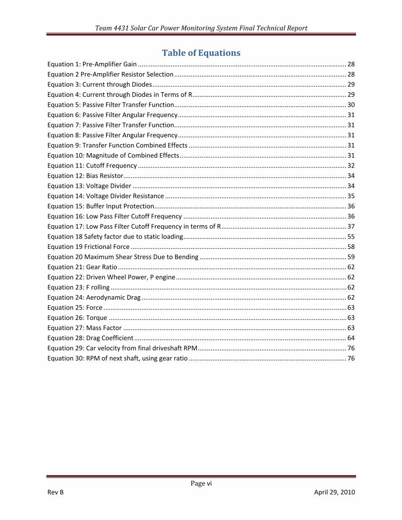
Table of Contents 1 Introduction .......................................................................................................................................... 9
1.1 Sponsor and Mentor ..................................................................................................................... 9
3.4 Preliminary Design Scoring and Selection ................................................................................... 19
3.5 Final Design ................................................................................................................................. 20
4 Final Design ......................................................................................................................................... 21
4.1 System Architecture .................................................................................................................... 21
4.2 Sensors and Processing ............................................................................................................... 24
5 System Build ........................................................................................................................................ 70
Team 4431 Solar Car Power Monitoring System Final Technical Report
Page 9 Rev B April 29, 2010
1 Introduction
1.1 Sponsor and Mentor The University of Arizona Solar Racing team has proposed a senior design project to design a solar vehicle power monitoring system for use on their solar race vehicle. Team 4431, Solar Power Monitoring System, has accepted the challenge to design and build such a system.
The design project will be guided through our sponsors: Sean Martinez, a mechanical engineer and graduate student, and Wei Ren Ng, an electrical engineer and graduate student. Additionally we have a faculty mentor, Clayton Grantham, who will help guide us throughout the design process.
1.2 Customer Background Our customer, the University of Arizona Solar Racing Team, has been competing in solar vehicle events since 1999. These events include the Sunrayce, Formula Sun, North American Solar Challenge and most recently the Shell Eco‐Marathon. Each of these races has a specific goal. The goals of each event can be categorized into two main types of racing: most efficient vehicle and quickest vehicle to the finish line. In order to best prepare for the races, the UA Solar Racing Team desires to evaluate vehicle power and efficiency to best configure the vehicle for the specific event they are competing in. In order to evaluate the vehicle, many factors must be monitored and characterized.
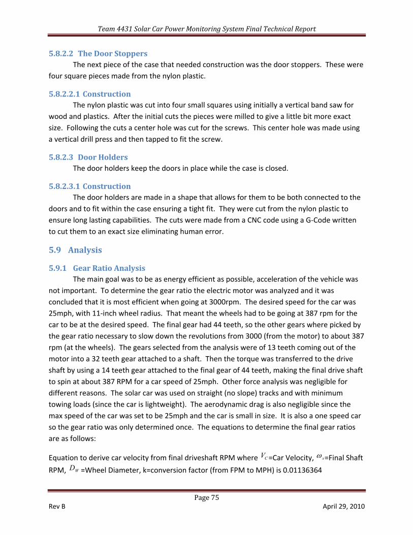
1.3 Meeting the Customer Need In order to meet the customer’s needs, Team 4431 will design a system to monitor the power usage of the UA Solar Car to support an effort to improve the electrical and mechanical efficiency of the vehicle. To accomplish this mission, both electrical and mechanical systems will need to be analyzed. Electrical systems to be considered are the solar arrays, batteries, motor performance both consuming and regenerating, and on‐board electronics. Collection of the electrical data will be achieved through a real‐time telemetry system with a goal of minimal power consumption due to the monitoring system component draws. Mechanical aspects that will be considered are vehicle mechanical efficiency of the rolling resistance through evaluation of alignment, applied horsepower and torque though evaluation of gear ratios and vehicle speed monitoring.
Team 4431 Solar Car Power Monitoring System Final Technical Report
Page 10 Rev B April 29, 2010
2 System Requirements
2.1 Discovering Requirements The requirements for this system were derived from the original proposal, meetings with the customer, and discussion with our mentor. The process of gathering requirements began with the initial customer needs statement for the project description. The team met and discussed the requirements to form questions for the sponsors in an attempt to discover additional requirements that may not have been specified initially. Once the questions were addressed by the sponsors the team began generation of the functional requirements. The functional requirements were reviewed with the sponsor and scored to establish a hierarchy of importance. Functional requirements were further broken down into sub‐requirements and finally into design parameters to define the subsystems.
2.2 Customer Attributes Customer attributes are the start of requirements definition for the project. Each customer attribute is developed into functional requirements to better describe how the system shall functionally meet the customer needs.
Customer attribute CA‐1, Monitor Solar Vehicle Power, is a stated requirement from the sponsors defining much of the scope of the project.
Customer Attribute CA‐2, Data Acquisition System with Telemetry, is a stated requirement from the sponsors which adds to the scope of CA‐1.
Customer Attribute CA‐3, Evaluate Mechanical Attributes, is a discovered requirement from the customer that was formed after meeting with the customer and learning about the mechanical capabilities of our team.
Customer attributes and their decomposition into functional requirements are illustrated in Figure 1, Figure 2, and Figure 3.
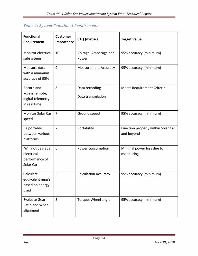
2.3 Functional Requirements Functional requirements are derived from customer attributes. The functional requirements are used to define sub‐requirements, known as design parameters, for which each of the sub‐system designs are developed to complete the overall design intent. From the functional requirements, preliminary designs are developed in an attempt to satisfy the customer needs. From all of the preliminary design ideas, an ideal final result is formed.
Functional requirements are derived from customer attributes. The summary of derived functional requirements is illustrated in Table 1.
Team 4431 Solar Car Power Monitoring System Final Technical Report
Page 11 Rev B April 29, 2010
Figure 1: Functional Decomposition of CA1
Team 4431 Solar Car Power Monitoring System Final Technical Report
Page 12 Rev B April 29, 2010
Figure 2: Functional Decomposition of CA2
Team 4431 Solar Car Power Monitoring System Final Technical Report
Page 13 Rev B April 29, 2010
Figure 3: Functional decomposition of CA3
Team 4431 Solar Car Power Monitoring System Final Technical Report
Page 14 Rev B April 29, 2010
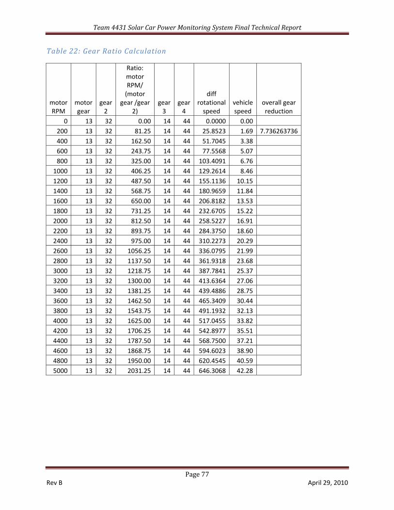
Table 1: System Functional Requirements
Functional Requirement
Customer Importance
CTQ (metric) Target Value
Monitor electrical subsystems
10 Voltage, Amperage and Power
95% accuracy (minimum)
Measure data with a minimum accuracy of 95%
9 Measurement Accuracy 95% accuracy (minimum)
Record and access remote, digital telemetry in real time
8 Data recording
Data transmission
Meets Requirement Criteria
Monitor Solar Car speed
7 Ground speed 95% accuracy (minimum)
Be portable between various platforms
7 Portability Function properly within Solar Car and beyond
Will not degrade electrical performance of Solar Car
6 Power consumption Minimal power loss due to monitoring
Calculate equivalent mpg’s based on energy used
5 Calculation Accuracy 95% accuracy (minimum)
Evaluate Gear Ratio and Wheel alignment
5 Torque, Wheel angle 95% accuracy (minimum)
Team 4431 Solar Car Power Monitoring System Final Technical Report
Page 15 Rev B April 29, 2010
2.4 Constraints Constraints are the envelope in which the system must operate. Through the development of the functional requirements, constraints become apparent. Constraints can be handed down by the customer, by law, regulation, or simply common sense. These constraints typically are categorized (but are not limited to) as performance, materials, safety or budget.
Constraints discovered throughout the development of the functional requirements were a combination of customer driven and common sense. A listing of specific constraints can be found in Table 2.
Table 2: Constraints
Constraints Parts of the Design Affected
Materials
• Weight should be less than 1% of total car weight (~8 lbs)
• Should consume less than 1 cubic foot of space
Weight: Entire system (sensors, wiring, communications box, antenna)
Size: Main communications box
Performance
• Range of signal transmission should be at least 1.5 miles
• System will be self powered
• The system should be operable over Arizona seasonal temperature
Range: Transceiver
Power: Entire system
Temperature: Entire system
Safety
• Will not interfere with safe operation of vehicle
Power: voltage, current levels
Budget
• Will be developed for under $2000
Cost: Entire system
Team 4431 Solar Car Power Monitoring System Final Technical Report
Page 16 Rev B April 29, 2010
2.5 Requirements Summary The overall system definition can be described through the functional requirements and constraints. Теория решения изобретательских задач (Teoriya Resheniya Izobretatelskikh Zadatch) or TRIZ is often used to ensure design parameters meet functional requirements however we felt this was not necessary due to the clear breakdown of customer attributes through to functional requirements and down to lower level design parameters.
In summary, the system shall:
• Monitor electrical subsystems and vehicle speed within an accuracy of 95% of the actual values, record and access remote digital telemetry in real time, be portable between various platforms and will not degrade the electrical performance of the vehicle in which it is installed
• Readout date on a remote computer ground station with the capability of analyzing the acquired data for equivalent miles per gallon (MPG) per Shell Eco‐Marathon methods
• Evaluate vehicle alignment, horsepower, torque and gear ratio
The system shall meet the above requirements without violating the following constraints:
• Not to exceed 1% of the vehicle weight (~8lbs), in less than 1 cubic foot of physical space
• Telemetry shall have a range of at least 1.5 miles
• Operate over Arizona seasonal temperature (20 – 120 degrees Fahrenheit)
• Will not interfere with safe vehicle operation
• Be designed and implemented for $2000 or less
Team 4431 Solar Car Power Monitoring System Final Technical Report
Page 17 Rev B April 29, 2010
3 Preliminary Designs and Selecting a Final Design
3.1 Developing a final design Development of the final design began with ensuring each design met the functional requirements. The team reviewed the requirements and ensured that each design satisfied the functional requirements.
In order to decide on a final design, the team went through a selection process involving both customers and mentor. To start, we came up with an ideal final result (IFR) comprised of the electrical and mechanical necessities as well as some “nice to have” features. We reviewed the IFR with the customer and recorded their recommendations and trade off ideas. We also consulted our mentor for his input from an electrical design aspect. After reviewing with both customer and mentor, the IFR was developed as shown in Figure 4.
3.2 Ideal Final Result
Figure 4: Ideal Final Result
Team 4431 Solar Car Power Monitoring System Final Technical Report
Page 18 Rev B April 29, 2010
3.3 Preliminary Designs Preliminary designs were developed to meet the requirements and were presented at the Preliminary Design Review (PDR). A summary of those designs is shown in Figure 5. For additional details of all aspects of each preliminary design, please see the PDR presentation in the Engineering Notebook on the Senior Design Website: http://proj498.web.arizona.edu/sites/default/files/498PDR%20Final.pptx
Team 4431 Solar Car Power Monitoring System Final Technical Report
Page 19 Rev B April 29, 2010
3.4 Preliminary Design Scoring and Selection A Pugh chart was developed to assist in selecting the final design. Upon reviewing the designs, complexity and innovation of the designs, and budget, the scores were recorded and are shown in Figure 6:
Weight Design 1 Design 2 Design 3
Sensor Design 10 0 + ‐
Telemetry 8 + + 0
Software 7 0 + 0
Alignment 6 0 + +
Total + 8 31 6
Total 0 23 0 15
Total ‐ 0 0 10
Overall Score 8 31 ‐4
Figure 6: Pugh Chart
The Pugh chart was developed using a “worse than / equal to / better than” approach, resulting in weighted scores across a simple “‐ / 0 / +” score which was totaled to determine the best attributes of each design. Rather than selecting one design in its entirety, each aspect of the designs were evaluated individually to allow the potential for a hybrid system using parts of each individual design. Upon final review of the best design attributes combined with available budget, we arrived at a final design.
Team 4431 Solar Car Power Monitoring System Final Technical Report
Page 20 Rev B April 29, 2010
3.5 Final Design
Figure 7: Final Design
The final design meets or exceeds all of the customer requirements however it does not include the in‐vehicle display.
Team 4431 Solar Car Power Monitoring System Final Technical Report
Page 21 Rev B April 29, 2010
4 Final Design
4.1 System Architecture
4.1.1 Overview Data is first gathered by sensors (some pre‐existing within the vehicle, some supplied by the project) and sent to the sensor hub. The sensor hub aggregates this sensor data and outputs the aggregated data to a ground station computer, via either wired (for test‐bench testing) or wireless (for in‐vehicle testing) telemetry. The ground station computer records the information and provides a real‐time visualization of the data. Data post‐analysis can then be performed directly on the ground station or on a separate computer. The actual data collected by the sensors were chosen to facilitate the analysis and optimization of the solar car vehicle. These sensors are described, at a high level, below. A graphical representation of the system architecture is shown in Figure 8:
Team 4431 Solar Car Power Monitoring System Final Technical Report
Page 22 Rev B April 29, 2010
Figure 8: Data Logging Architecture
Team 4431 Solar Car Power Monitoring System Final Technical Report
Page 23 Rev B April 29, 2010
4.1.2 Sensors Data is collected from a variety of sensors with different interfaces. Some of these
sensors are built into the vehicle; others are provided by our project.
4.1.2.1 V/I Sensors Voltage/Current (V/I) sensors sample instantaneous voltage and current and are a
custom design by our team. From the voltage and current measurements, instantaneous
power can be determined ( IV=P ), as well as total energy usage ( Pdt=W ∫ ). These sensors
communicate with the sensor hub via the CAN (controller‐area network) 2.0 A bus. Four of these devices were created: 1. Motor power line sensor 2. 12 V subsystem sensor 3. 24 V subsystem sensor 4. Spare sensor
4.1.2.2 Speed Sensor The speed sensor samples the instantaneous speed of the vehicle. This sensor is
provided by our team. The speed sensor communicates with the sensor hub via the CAN bus.
4.1.2.3 Tilt Sensor The tilt sensor samples the tilt of the vehicle in order to; for example, provide
information on the grade of an incline the vehicle is traversing. This sensor is provided by our team and communicates over the CAN bus.
4.1.2.4 MPPTs The maximum power point trackers (MPPTs) are already existent within the vehicle and
are used to provide the maximum power output from solar panel sub‐arrays. The MPPTs provide voltage and current measurements from the solar sub‐arrays and communicate this information to the sensor hub via the CAN bus.
4.1.2.5 BPS The battery protection system (BPS) is also already existent within the vehicle and is
used to protect the vehicle’s battery cells from adverse conditions such as overheating, short‐circuiting, and under‐voltage. The BPS measures total battery current, individual cell voltages, and temperature at several locations within the battery compartment. This information is communicated to the sensor hub via an RS‐232 serial link.
Team 4431 Solar Car Power Monitoring System Final Technical Report
Page 24 Rev B April 29, 2010
4.1.3 Sensor Hub The sensor hub provides an interface to the various sensors and aggregates their data.
This aggregated data is then sent out to the ground station computer in a serial stream. The serial stream must efficiently pack data into the fewest bits possible to be compatible with slow serial baud rates (such as 9600 Baud/s) that may be required by the telemetry hardware.
For wired telemetry, the sensor hub may be directly connected to the ground station computer via a serial cable. For wireless telemetry, a radio modem may be connected to the sensor hub and another radio modem connected to the ground station computer. These modems act to "tunnel" serial data between the sensor hub and ground station computer nodes.
The sensor hub has the ability to interface with one RS‐232 serial device (e.g. the BPS) and up to 13 CAN bus‐equipped devices (this device limitation is due to the number of physical connectors). The sensor hub will also provide power to all sensors designed or supplied by the project.
4.1.4 Ground Station Computer The ground station computer (GSC) is a general purpose computer (e.g. a PC) running
data capture and visualization software. The GSC collects the serial data stream sent by the sensor hub (either via wired or wireless telemetry), parses the stream for sensor data, records the data, and displays the information on the user interface in real‐time.
The recorded data can be saved to be analyzed later on the GSC or on a different computer. These analyses can then be used to perform optimizations on the actual solar car vehicle.
4.2 Sensors and Processing
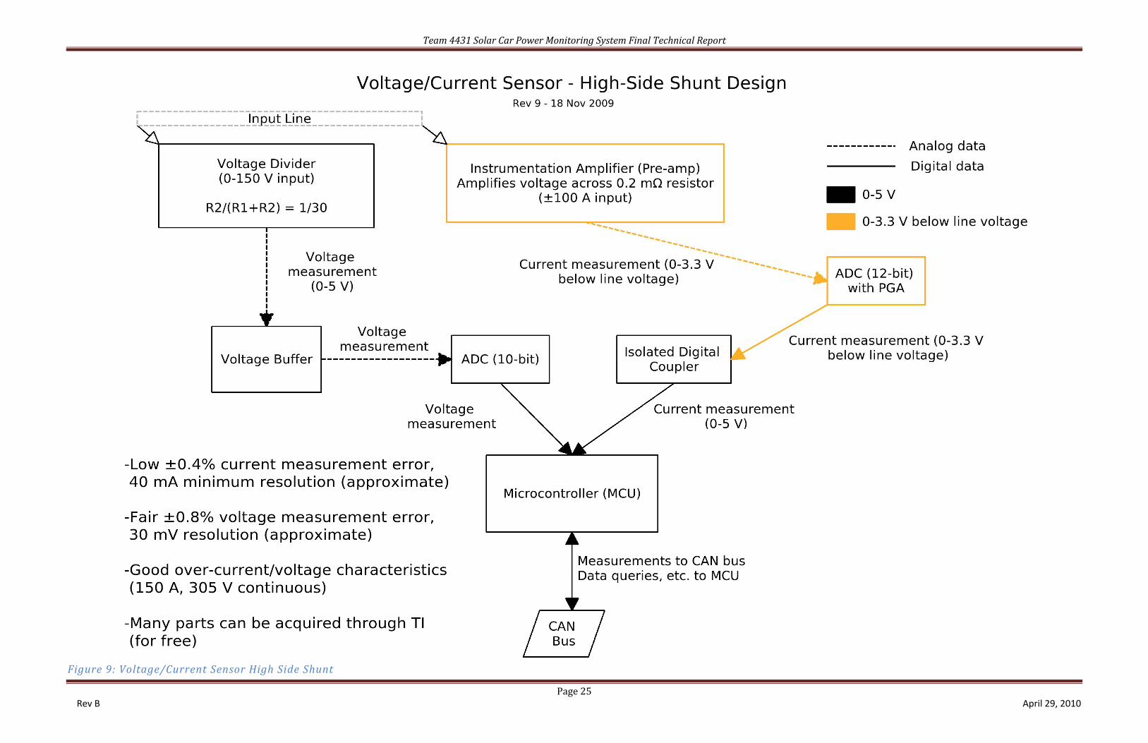
4.2.1 V/I Sensor Circuitry Description Sensor block diagram is shown in Figure 9: Sensor schematic is shown in Figure 10:
Team 4431 Solar Car Power Monitoring System Final Technical Report
Page 25 Rev B April 29, 2010
Figure 9: Voltage/Current Sensor High Side Shunt
Team 4431 Solar Car Power Monitoring System Final Technical Report
Page 26 Rev B April 29, 2010
Figure 10: V/I Sensor Schematic
Team 4431 Solar Car Power Monitoring System Final Technical Report
Line In Positive current input from high side line ( V1500− , A±100 )
Line Out Positive current output from high side line ( V1500− , A±100 )
CANH, CANL CAN bus communications lines ( V50− nominal, V±36 maximum continuous)
VBAT Power source ( V305.8− , reverse bias protected up to ‐30 V)
4.2.1.2 Overview The Voltage/Current (V/I) sensor is needed to measure instantaneous voltage and current values from power lines within a vehicle. From these voltage and current samples, instantaneous power delivered by the line can be calculated. The calculated power measurement total error must be less than 5%. To achieve this, the voltage and current measurements that make up this figure must have an even lower percentage error. Additionally, the V/I sensor must be portable across many different vehicle types so assumptions about the physical layout of the vehicle and vehicle wiring must be minimized.
4.2.1.3 Connectors The power and data connector ( 1JP ) supplies power to the V/I sensor and also provides
access to the two CAN communication lines (CANH and CANL). The connector is an RJ‐45 connector as the intended cabling is CAT5 UTP patch cable. The cabling was chosen to
accommodate the suggested Ω120 characteristic impedance of the CAN bus lines and as the twisted‐pair design of CAT5 cabling maximizes the noise‐canceling capability of the CAN bus’ differential signal communications. CAT5 UTP cable is readily available due to its use as
Ethernet patch cabling. The ISP connector ( 2JP ) allows for in‐system programming of the
ATtiny261A microcontroller (MCU).
4.2.1.4 General Voltage Regulation A raw battery input voltage (5.8 to V30 ) is regulated to V5 with the 6U linear
regulator. 2D is present to protect the circuitry against negative voltages of up to V30− . This
negative voltage could be caused, for example, by a battery being connected with a reversed polarity.
A shunt regulator (to produce a floating ground) and an inverter are also used within the circuit but are directly related to the current sensing circuitry and are thus described in the Current Sensing Circuitry section.
Team 4431 Solar Car Power Monitoring System Final Technical Report
Page 28 Rev B April 29, 2010
4.2.1.5 V/I Sensor Component Sizing
4.2.1.5.1 CurrentMeasure Shunt Resistor shuntR was sized as small as possible to minimize power dissipation from the line being
measured. From readily available suppliers, mΩ=Rshunt 0.2 was the smallest resistor available.
This results in a respective full‐scale voltage of mV± 20 ( iR=v ) across the resistor at the peak
current of A±100 . At this peak current, shuntR will dissipate W2 ( Ri=P 2 ).
Table 4: V/I Sensor Shunt Resistor
Component Value Tolerance
Rshunt 0 . 2 mΩ 1%
4.2.1.5.2 1U PreAmplifier Gain
Due to component tolerances (mainly the 5% tolerance of zener 1D ) and a safety
margin, the current‐sensing circuitry is designed to operate with a floating ground (FGND) with
a minimum voltage of V3 below the LINE_IN voltage. A full scale input of A100 through the
mΩ0.2 shuntR will produce mV20 across the resistor. As the output is split by an offset
between the rails (to allow for bi‐directional current sensing), the mV20 signal must be
amplified to V1.5 to span across the minimum ( V3 ) voltage range of the FGND circuitry. In
order to do this, the desired gain of 1U was calculated: VV=mVV=G ∕75
201.5
.
The gain of the INA326/7 amplifier ( 1U ) is given by:
1
22I
I
RR=G
Equation 1: PreAmplifier Gain
The INA326/7 datasheet suggests that 1IR be valued no less than kΩ2 and be sized based on
the equation (personalized to the schematic):
μAV
=R maxRshuntI 12.5
_1
Equation 2 PreAmplifier Resistor Selection
Team 4431 Solar Car Power Monitoring System Final Technical Report
Page 29 Rev B April 29, 2010
With V Rs hunt _ma x= 20 mV (the full‐scale voltage across shuntR at A100 ), Equation 2 produces
kΩ=RI 1.61 . As this value is less than the minimum suggested value of kΩ2 , the final value of
1IR is set to kΩ=RI 21 .
Re‐arranging Equation 1, it can be determined that kΩ=RI 752 produces the desired gain of
VV=G ∕75 .
Table 5: PreAmplifier Resistor Selection
Component Value Tolerance RI 1 2 k Ω 0.1% RI 2 7 5 k Ω 0.1%
4.2.1.5.3 SolidState Relay Control Line Resistors 7R and 8R limit the current supplied to the 12U and 13U AQW610EH solid‐state relays
(SSRs). The AQW610EH datasheet specifies a minimum of mA3 is required for the control LEDs (on the IC) to ensure the switching of the relay. These LEDs have a maximum voltage drop of
V1.5 . Although the LED will drop less than this voltage at lower currents ( V1.14 typical with a
diode current of mA5 ), this V1.5 value is used to provide a safety margin.
The control lines are designed so that a single resistor is in series with two control LEDs. Putting two LEDs in series saves on current consumption from the control line (which is driven
by an MCU that can drive a maximum of mA20 from a GPIO pin).
The current through the diodes can be modeled by the following equation ( 8R can be
substituted for 7R ):
7
_ 1.52R
V)(V=i INVI
d
−
Equation 3: Current through Diodes
Re‐arranging Equation 3:
d
INVI
iV)(V
=R=R1.52_
87
−
Equation 4: Current through Diodes in Terms of R
Team 4431 Solar Car Power Monitoring System Final Technical Report
Page 30 Rev B April 29, 2010
INVIV _ is the voltage on the control line (net I_INV) that is powered by the MCU. No
current flows through the control LEDs when this voltage is low (assumed V0 ) so we are
interested in the other voltage level from the digital output: when INVIV _ is high (assumed at
V5 , although this voltage may be slightly lower).
The LED on‐current must be between mA3 and mA50 to operate properly and must be
less than mA10 (per control line) for the MCU to drive the control lines. From this, mA5 was somewhat arbitrarily chosen as the desired LED current. Knowing this, the resistors can be sized using Equation 3:
Using the value of Ω=R=R 39087 and Equation 3, mAid 5.128≈ and the current drawn from
the MCU GPIO pin is approximately mA10.256 , well below the mA20 maximum.
The LED currents are still well above the mA3 minimum when 5% resistor tolerances are taken into account.
4.2.1.5.4 TwoPole LowPass Filter on 1U PreAmplifier Output
1R , 1C , 2IR , and 2IC form a second‐order, two‐pole low‐pass filter on the output of
the 1U pre‐amplifier. The following describes the characterization of the filter and component
sizing.
4.2.1.5.4.1 Filter Characterization
4.2.1.5.4.1.1 Passive Filter 1
1R and 1C form a passive, single pole low‐pass filter (LPF) with transfer function:
sCR+=(s)H
111 1
1
Equation 5: Passive Filter Transfer Function
Ω=R=RΩ=mAVV=R=R valueNearest 390400
535
875%
87 →−
Team 4431 Solar Car Power Monitoring System Final Technical Report
Page 31 Rev B April 29, 2010
and 3dB cutoff angular frequency:
111
1CR
=ωo
Equation 6: Passive Filter Angular Frequency
4.2.1.5.4.1.2 Passive Filter 2
Similarly, 2IR and 2IC form a passive, single pole LPF with transfer function:
sCR+=(s)H
II 222 1
1
Equation 7: Passive Filter Transfer Function
and 3dB cutoff angular frequency:
222
1
IIo CR=ω
Equation 8: Passive Filter Angular Frequency
4.2.1.5.4.1.3 Combined Effects The design of the instrumentation amplifier (INA326/7) combines these two LPFs into an equivalent LPF with transfer function:
s)CR+s)(CR+(=(s)(s)HH=H(s)
II 221121 11
1
Equation 9: Transfer Function Combined Effects
The two poles of H(s) reside in the left‐half plane, so we can safely set jω=s . The resulting
magnitude equation is:
21122
2221211
1=)(ω)CR+ωC(R+)ωCCRR(
|jωH|IIII−
Equation 10: Magnitude of Combined Effects
To find the 3dB cutoff frequency ( oω ), set 2
1=|)H(jω| o and solve to get:
Team 4431 Solar Car Power Monitoring System Final Technical Report
Page 32 Rev B April 29, 2010
22121
222
211
22121
422
411
26
)CCR(R)C(R)C(R)CCR(R+)C(R+)C(R
=ωII
IIIIIIo
−−
Equation 11: Cutoff Frequency
4.2.1.5.4.2 Component Value Determination The 12‐bit ADC ( 2U ) will sample the output of the 1U INA at 250 SPS. To prevent
aliasing, the low‐pass filter on the output of the INA should filter out any frequencies above at
least Hz=1252
250 (see the Nyquist‐Shannon sampling theorem). As a safety factor, a slightly
lower cutoff frequency of Hz=fo 100 ( s)radπ(=πf=ω oo ∕10022 ) is desired for the filter.
The value of 2IR is determined by the desired gain of the amplifier, and is therefore
known prior to the sizing of the other components present in the filter.
To determine the values of 1R , 1C , and 2IC :
1. Make an educated guess (based on the INA326/7 datasheet) and let μF=C 11
2. Assume 21 oo ω=ω and assume (for now) that 21 IR=R (pretending the value of 2IR is
unknown) and that 21 IC=C
3. With s)radπ(=ωo ∕1002 (i.e. 100 Hz), the desired cutoff frequency, and μF=C=C I 121 ,
plug into Equation 11 and solve for 1R :
4. Using Equation 6, we can determine s)radπ(ωo ∕159.154921 ≈
5. Since kΩ=RI 752 (chosen to obtain desired gain of the amplifier) and 21 oo ω=ω (ideally),
we can determine 2IC by using Equation 8:
6. Using these final values for 1R , 2IR , 1C , and 2IC (see Table 7) and Equation 11, the
kΩ=RΩR valueNearest 11024.3 15%
1 →≈
nF=CnFC IvalueavailableNearest
I 1313.3 2
2 →≈
Team 4431 Solar Car Power Monitoring System Final Technical Report
Page 33 Rev B April 29, 2010
actual 3dB cutoff frequency of the overall LPF can be estimated (assuming ideal components) at:
Table 7: Resistor and Capacitor Selection Component Value Tolerance
R1 1 k Ω 5%
RI 2 75 k Ω 0.1%
C1 1 μ F 10%
C I 2 1 3 n F 10%
4.2.1.5.5 Floating Ground Regulator Zener Diode and Bias Resistor The two components of the floating ground (FGND) regulator that can be sized are: the
zener diode, 1D , and the bias resistor, biasR .
4.2.1.5.5.1 Zener Diode The zener diode, 1D , was sized to have a zener voltage of V3.9 ; when reverse biased,
the diode will have a nominal voltage of V3.9 across the terminals. This voltage was chosen so
that, when considered with the estimated VV QBE 0.63_ ≈ , FGND will sit approximately V3.3
below the voltage of LINE_IN. All ICs on FGND are compatible with this V3.3 supply.
An additional concern with the sizing of this zener diode is uncovered when the LINE_IN
voltage is low. Current measurement must function properly on line voltages down to V0 so
the V5− supply was introduced. 2Q sits between the diode and the V5− supply and is
desired to maintain operation in the active region. The voltage drop caused by these BJTs can
be a minimum of VV SatQCE 0.32__ ≈ . The V0.3 minimum collector‐emitter voltage of 2Q plus
the V3.9 drop across the zener diode require at least V4.2 , leaving an extra V0.8 between
the V0 LINE_IN and the V5− supply for component tolerances and as a safety margin.
4.2.1.5.5.2 Bias Resistor The zener diode produces a V3.9 zener voltage when reverse biased at μA250 . To
account for current pulled in through the base of 3Q (approximately μA50 peak) and to
provide a safety margin, the current mirror biasing the zener diode was desired to pull about
Hz=s)radπ(ωo 102.43∕102.432≈
Team 4431 Solar Car Power Monitoring System Final Technical Report
Page 34 Rev B April 29, 2010
μA350 . The value of biasR controls the amount of current drawn through the mirror and this
current is approximated by:
bias
QBEbias i
VV)(V=R 1_50 −−−
Equation 12: Bias Resistor
This equation ignores the 1Q and 2Q base currents.
Assuming V=V QBE 0.71_ (in reality, this value will likely be slightly smaller),
kΩ=Rbias 12 produces an μAibias 358.3≈ and is acceptable as a resistor with 5% tolerance (
biasi will drop to no lower than μA341.2 ).
Table 8: Resistor and Diode Selection
Component Value Tolerance
D1 3 .9 V 5%
Rbi as 12 kΩ 5%
4.2.1.5.6 Voltage Sensing Input Resistors The input of the voltage sensing circuitry contains three resistors: 1VR , 2VR , and 2R .
4.2.1.5.6.1 Voltage Divider 1VR and 2VR form a voltage divider to divide the V1500− input line voltage (LINE_IN)
down to the V50 − level of the voltage buffer ( 5U ) and MCU with ADC ( 7U ). Due to power
supply tolerances, the V5 power supply may have a minimum voltage of V4.9 (‐2% error).
Additionally, the OPA340 buffer ( 5U ) can be expected to output a maximum of mV50 below
the supply rail. Thus, we must divide a V150 signal down to V4.85 . This voltage divider equation is:
VV=
R+RR
VV
V
1504.85
21
1
Equation 13: Voltage Divider
kΩ=RkΩμAVV=R bias
valueNearestbias 1212.286
3500.75 5%
→≈−
Team 4431 Solar Car Power Monitoring System Final Technical Report
Page 35 Rev B April 29, 2010
It is also desired to have a total voltage divider resistance of about MΩ1 . This value is
large enough to limit current draw from LINE_IN to μA150 and small enough to limit electrical
noise produced the by divider resistors.
MΩ=R+R VV 121
Equation 14: Voltage Divider Resistance
Solving Equation 13 and Equation 14 simultaneously, we find:
However, plugging the results in:
we find the sizing to produce an output voltage greater than maximum V4.85 with an input of
V150 . To fix this, 2VR is bumped up to the next 0.1% resistor value: kΩ=RV2 976 . Trying
again:
This is less than the V4.85 maximum (even when 0.1% tolerances are included), so the value of
kΩ=RV2 976 is the final value for the resistor.
Table 9: Resistor Selection
Component Value Tolerance
RV 1 3 2 . 4 k Ω 0.1%
RV 2 976 kΩ 0.1%
kΩ=RkΩR VvalueNearest
V 32.432.333 10.1%
1 →≈
kΩ=RkΩR VvalueNearest
V 965967.667 20.1%
2 →≈
VkΩ+kΩ
kΩ=R+R
RVV
V 4.8796532.4
32.4V 150V 15021
1 ≈
VkΩ+kΩ
kΩ=R+R
RVV
V 4.8297632.4
32.4V 150 V 15021
1 ≈
Team 4431 Solar Car Power Monitoring System Final Technical Report
Page 36 Rev B April 29, 2010
4.2.1.5.6.2 Buffer Input Protection 2R protects the (non‐inverting) input of the 5U buffer from high‐voltage transients.
kΩ=R 5.12 was chosen based upon the recommendation of the OPA340 datasheet. While the
datasheet specifies a kΩ5 value, kΩ5.1 is the nearest 5% resistor value.
The 5U (OPA340) inputs are diode‐clamped to the power supply rails and any voltage of 5 00 mV above the rail (i.e. V5.5 ) must be current‐limited to mA10 .
V+)mA)(R(=Vmax 5.510 2
Equation 15: Buffer Input Protection
From Equation 15, kΩ=R 5.12 protects the input of the 5U buffer from voltages up to
V=Vmax 56.5 . Dividing this result by the attenuation factor provided by the voltage divider 1VR
and RV 2 , the maximum LINE_IN voltage the 5U buffer can handle is calculated:
Table 10: Resistor Selection
Component Value Tolerance R2 5.1 kΩ 5%
4.2.1.5.7 OnePole LowPass Filter on 5U (OPA340) Output
Following the reasoning in section 4.2.1.5.4.2, the low‐pass filter on the output of the
5U voltage buffer has a desired cutoff frequency of s)radπ(=ωo ∕1002 .
The filter is a simple passive RC low pass‐filter with cutoff frequency given by:
63
1CR
=ωo
Equation 16: Low Pass Filter Cutoff Frequency
Due to the medium input resistance (tens of kΩ ) of the ADC input, the value of 3R is
desired to be small to mitigate the voltage divider effect of 3R in series with the ADC’s input
kVkΩ
kΩ+kΩV=V maxmaxINLINE 1.758532.4
97632.4__ ≈
Team 4431 Solar Car Power Monitoring System Final Technical Report
Page 37 Rev B April 29, 2010
resistance. As shown by Equation 16, a larger‐valued 6C results in a lower‐valued 3R for the
same oω . The size of 6C is somewhat arbitrarily limited to a maximum of μF10 in order to
limit the physical capacitor size and to limit capacitor parasitics that limit the capacitor’s response at higher frequencies (e.g. equivalent‐series inductance, ESL).
Rearranging Equation 16:
oωC=R
63
1
Equation 17: Low Pass Filter Cutoff Frequency in terms of R
Using Equation 17 with s)radπ(=ωo ∕1002 and C6= 1 0 μ F :
Table 11: Resistor and Capacitor Selection
Component Value Tolerance R3 1 6 0 Ω 5% C1 1 0 μ F 10%
4.2.1.5.8 V5 Voltage Regulator External Components
4.2.1.5.8.1 Decoupling Capacitors RIC smoothes the input voltage ripple and is set to μF=CRI 1 , the value
recommended by the LP2950 datasheet. ROC smoothes the output (regulated) voltage ripple
and is recommended to be a minimum of μF1 for loads drawing mA100 . The load of the
circuit is a expected to draw much less current, so the minimum value of the capacitor can be
reduced. Still, to limit the number of capacitor values used, μF=CRO 1 as well.
Table 12: Capacitor Selection
Component Value Tolerance CRI 1 μ F 10% CRO 1 μ F 10%
4.2.1.5.8.2 LED Resistor PWRR limits the current running through the power‐on LED, PWRD . About mA10 of
current (estimated as a good balance between luminance and power consumption) is desired
Team 4431 Solar Car Power Monitoring System Final Technical Report
Page 38 Rev B April 29, 2010
through the LED. The LED should drop about V1.4 when forward biased. The value of PWRR is
calculated using:
However, as Ω=R=R 39087 , the number of different‐valued resistors used in the
design can be reduced by increasing PWRR to Ω390 . With this value, the current through the
LED can be calculated:
With a 5% resistor tolerance, mAiDPWR 8.791≈ is the minimum LED current that can be
expected. These currents are acceptable so Ω=RPWR 390 .
Table 13: Resistor and Capacitor Selection
Component Value Tolerance RPW R 39 0 Ω 5% CRI 1 μ F 10% CRO 1 μ F 10%
4.2.1.5.9 4U Inverter Capacitors
The capacitors NIC (input voltage ripple), NOC (output voltage ripple), and NFLYC
(flying capacitor) for the 4U inverter are all sized to μF1 based upon the general use
recommendations of the TPS60400 datasheet.
Table 14: Capacitor Selection
Component Value Tolerance CN I 1 μ F 10% CNO 1 μ F 10% CN F LY 1 μ F 10%
4.2.1.5.10 General Pullup Resistors
4.2.1.5.10.1 CI 2 Resistors The CI 2 lines are pulled high (as is specified by the protocol) by ASDAR , ASCLR , BSDAR ,
and BSCLR , all valued at kΩ10 . The CI 2 communication will be conducted at low bus speeds
so the maximum recommended value of kΩ10 is used (at higher bus speeds, the RC time
Ω=mAVV=RPWR 360
101.45 −
mAΩVV=iDPWR 9.231
3901.45
≈−
Team 4431 Solar Car Power Monitoring System Final Technical Report
Page 39 Rev B April 29, 2010
constant of the line may limit data rates). The use of this large value for the pull‐up resistors
reduces power consumption of the CI 2 bus versus smaller valued resistors.
Table 15: Resistor Selection
Component Value Tolerance RAS DA 10 k Ω 5% RAS C L 10 k Ω 5% RBS DA 10 k Ω 5% RBS C L 10 k Ω 5%
4.2.1.5.10.2 Reset Resistor The RESET line (active low) is held high by 6R . The RESET line is used both to reset the
7U microcontroller and to debug the MCU via debugWIRE. From the ATtiny261A datasheet,
the recommended pull‐up resistor on the RESET line when using debugWIRE is between kΩ10
and kΩ20 . As the CI 2 lines already use kΩ10 pull‐ups, kΩ=R 106 was chosen to limit the
number of resistor values used in the design.
Table 16: Resistor Selection
Component Value Tolerance R6 10 k Ω 5%
4.2.1.5.10.3 Pre‐Amplifier Enable Resistor 4R pulls the 1U pre‐amplifier enable line high during normal operations. This line is
pulled low by the alert pin of the 2U ADC to disable 1U in order to conserve power between
ADC sampling. As all other pull‐up resistors are valued at kΩ10 , kΩ=R 104 was also chosen to
limit the number of resistor values used in the design. 4R will draw about μA330 when the
enable line is pulled low.
Table 17: Resistor Selection
Component Value Tolerance R4 10 k Ω 5%
4.2.1.5.11 IC Supply Decoupling Capacitors Decoupling capacitors are placed across the power nets of most integrated circuits (ICs) present in the design in order to smooth out power line noise and ensure proper operation of the ICs. These capacitors must be placed near power pins of each IC to be effective; non‐
Team 4431 Solar Car Power Monitoring System Final Technical Report
Page 40 Rev B April 29, 2010
idealities of traces on a physical circuit board negate the effects of these capacitors if placed far
away. As a rule‐of‐thumb, these capacitors are valued at μF0.1 . The ICs with suggested
decoupling capacitors are no different; the datasheets specify μF0.1 capacitors. Hence,
μF=C=C=C=C=C=C=C=C 0.1109875432 .
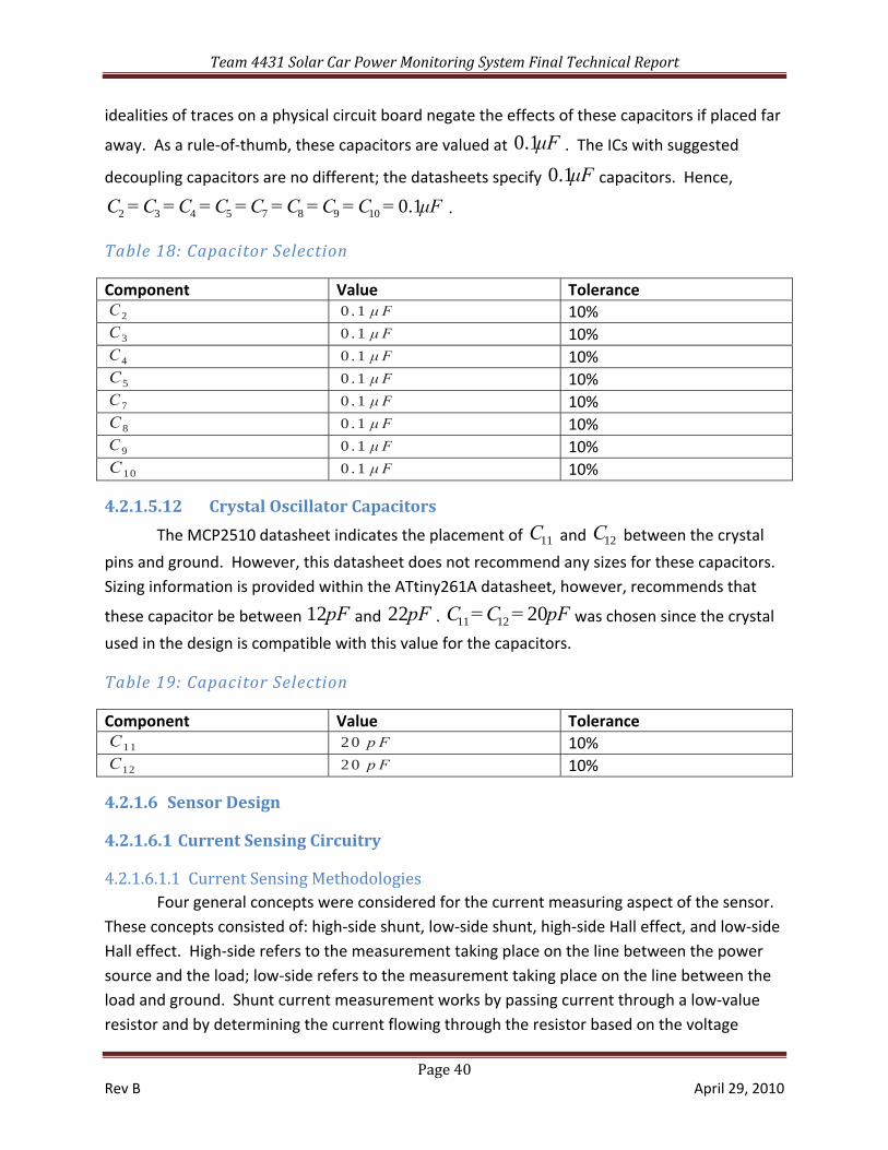
Table 18: Capacitor Selection
Component Value Tolerance C2 0 . 1 μ F 10% C3 0 . 1 μ F 10% C4 0 . 1 μ F 10% C5 0 . 1 μ F 10% C7 0 . 1 μ F 10% C8 0 . 1 μ F 10% C9 0 . 1 μ F 10% C10 0 . 1 μ F 10%
4.2.1.5.12 Crystal Oscillator Capacitors
The MCP2510 datasheet indicates the placement of 11C and 12C between the crystal
pins and ground. However, this datasheet does not recommend any sizes for these capacitors. Sizing information is provided within the ATtiny261A datasheet, however, recommends that
these capacitor be between pF12 and pF22 . pF=C=C 201211 was chosen since the crystal
used in the design is compatible with this value for the capacitors.
Table 19: Capacitor Selection
Component Value Tolerance C11 20 p F 10% C12 20 p F 10%
4.2.1.6 Sensor Design
4.2.1.6.1 Current Sensing Circuitry
4.2.1.6.1.1 Current Sensing Methodologies Four general concepts were considered for the current measuring aspect of the sensor. These concepts consisted of: high‐side shunt, low‐side shunt, high‐side Hall effect, and low‐side Hall effect. High‐side refers to the measurement taking place on the line between the power source and the load; low‐side refers to the measurement taking place on the line between the load and ground. Shunt current measurement works by passing current through a low‐value resistor and by determining the current flowing through the resistor based on the voltage
Team 4431 Solar Car Power Monitoring System Final Technical Report
Page 41 Rev B April 29, 2010
across the resistor, using Ohm’s Law ( Rv=i ∕ ). Hall effect current measurement utilizes the effects of a permanent magnet interacting with the magnetic field of current flowing through a conductor to create a voltage which is proportional to the amount of current flowing through the conductor.
To measure voltage on the line, the sensor must be connected on the high side of the load (the load value is not known). This lowers the attractiveness of the low‐side current measurement option as the low‐side option would require one low‐side line in, one low‐side line out, and a line tapping into the high‐side cabling. This extra line from the high‐side cabling to the sensor decreases the ease‐of‐installation of the sensor and may not be practical if the low‐side and high‐side lines are not in close proximity. The high‐side current measuring option does not have this problem and requires only one high‐side line in and one high‐side line out. Fewer assumptions about the wiring of the vehicle are needed than with the low‐side current measuring option.
Hall effect sensors that were researched and that met the requirements of the ± 1 0 0 A range of line current were limited to an error of 5± % over operating conditions, meaning the voltage measurement would have to be 100% accurate for the device to meet the functional requirements of the design. Shunt current measurement, however, can measure current with a total error of less than 1%.
From these observations, the high‐side shunt current measurement concept was chosen for the V/I sensor design.
4.2.1.6.1.2 Current Sensing Design The current measurement circuitry resides on a floating ground (FGND), which is
approximately VV 3.33.2 − below the voltage of LINE_IN at all times, due to limitations of the common‐mode voltage range that can be safely handled by available instrumentation
amplifiers (INAs). No readily available INA could handle the V150 common‐mode line voltage found in the application.
shuntR is a mΩ0.2 current shunt resistor with a full scale voltage (at A±100 ) of mV± 20
( W2 ). The voltage across shuntR is differentially amplified by a factor of VV ∕75 by the INA
pre‐amplifier, 1U . The gain of VV ∕75 allows for a floating ground to be used (explained
below) that is a minimum of V3.0 below line level ( V3.3 below line level is desired but this
V3.0 takes into account component tolerances). This amplified signal is added to an offset
voltage of FGND)IN(LINE=Voff −_21
from the 11U rail splitter. This bias voltage allows
bidirectional current sensing from the INA. The INA was chosen as it can handle an input of
mV100 over the positive supply voltage, allowing it to operate on the floating ground and still handle "negative" current. The amplified signal superimposed on the bias is then fed into a 12‐
Team 4431 Solar Car Power Monitoring System Final Technical Report
Page 42 Rev B April 29, 2010
bit ADC with PGA ( 2U ). The PGA of 2U can amplify the incoming signal up to VV ∕16 ,
allowing for a greater dynamic resolution of the current sensor (i.e. the voltages produced by smaller currents can be amplified even more, resulting in a greater resolution at smaller
currents). After the PGA, the voltage signal is digitized by 2U ’s 12‐bit ADC. As the main
microcontroller (that collects the current data) of the sensor is running at the V50 − level, the
ADC’s CI 2 output signal (FGND level) must be passed through an isolated digital coupler,
which isolates the FGND circuitry from the V50 − circuitry while still allowing the digital data to be transferred.
The circuitry on this floating ground will draw an estimated maximum of mA10.5 from
the line which it is measuring (LINE_IN). A majority of this current (about mA5.5 ) is drawn by
the CI 2 bus and the CI 2 isolation circuitry. To conserve power on the floating ground line,
the ADC’s alert pin is pulled low (drawing about μA330 ) and the INA is put into a "sleep"
mode, where it draws a typical current of μA2 versus the typical INA operating current of
mA2.4 . To deal with the fact that FGND is not a stable reference and to remove the bias errors
associated with all of the current measuring analog front‐end circuitry, solid‐state relays (SSRs),
12U and 13U , are used to allow the inputs of the 1U INA to be "switched". When switched,
the non‐inverting input (which is normally connected to the "top" of shuntR ) is connected to the
"bottom" of shuntR and the inverting input (which is normally connected to the "bottom" of
shuntR ) is connected to the "top" of shuntR . A measurement of the amplified voltage will be
taken with the inputs "normal" and then, immediately after, the inputs to the INA will be switched and another measurement will be taken. From these two measurements, the signal offset (needed for the bidirectional sensing capability) that is present at the ADC input can be determined and the actual measurement voltage can be properly calculated. The control signals for these SSRs can be directly driven from a digital output pin of the MCU due to the electrical isolation between the control and switch circuitry within the relays. The pin must
only source mA10.3∽ to the relay controls when the line is raised high and A0 when the control line is low.
FGND is generated by a shunt regulator comprised of 1Q ‐ 3Q , 1D , and biasR . The
V3.9 zener diode, 1D , "hangs" off of the LINE_IN line, providing a reference voltage of V3.9
below the line voltage. The basic current mirror formed by 1Q ‐ 2Q and biasR generates a
current of about uA360 that biases 1D over the range of line voltages. The ground current of
the devices on the floating ground is routed through the collector‐emitter of 3Q so that the
Team 4431 Solar Car Power Monitoring System Final Technical Report
Page 43 Rev B April 29, 2010
majority of the bias current goes through 1D (and not the load). The BEV voltage of
approximately V0.6− to V0.7− raises the actual FGND value to about V3.2 to V3.3 below the LINE_IN line voltage.
To bias 1D , a simple current mirror was chosen over a more advanced current source,
such as a full Wilson current source, as the 12U and 13U SSR solution removes any offset
voltage errors within the current sensing circuitry from the final data. A large source of this
offset error is the changing of the voltage across 1D due to bias current fluctuations, caused in
part by changing line voltages and second‐order behaviors of the BJTs. These fluctuations impact the value of FGND and, therefore, change the line‐split offset voltage of the INA. A more advanced current source would reduce these fluctuations but not eliminate them, as the SSR
solution does. Therefore, a simple current source is all that is needed to bias 1D (with the SSR
solution in use).
The FGND shunt regulator is referenced to V5− rather the GND to accommodate an
FGND below V0 . This scenario occurs when the LINE_IN line voltage drops below V3.2 or
V3.3 and the presence of the V5− reference allows the current sensing circuitry to operate
on LINE_IN line voltages down to V0 . The V5− is generated by the inverter 4U .
4.2.1.6.2 Voltage Sensing Circuitry The voltage sensing circuitry is based upon a simple voltage divider ( 1VR and 2VR ) and
unity‐gain voltage buffer ( 5U ). The voltage divider divides the input line voltage ( V1500− ) to
the range of approximately V50 − , a 30∕1∽ ratio. The actual ratio is a bit lower (i.e.
32.13∕1∽ ) to compensate for component non‐idealities, such as a 2% error in the V5 voltage regulator that supplies power to the buffer and microcontroller. Current drawn through the
voltage divider at the maximum line voltage of V150 is uA149∽ . As both 1VR and 2VR will
be constructed using the same technologies and should have similar device characteristics (except for resistance), the two resistors should experience roughly the same temperature and any effects of temperature should affect both resistors in approximately the same way. If, for
example, temperature changes cause the value of 1VR to increase by 0.05%, the same
temperature effects should also cause the value of 2VR to increase by about 0.05%. These
changes cancel each other out within the voltage divider ratio, causing the ratio to remain the same.
2R protects the 5U op‐amp from voltage spikes on the line.
The buffered output of the divided voltage signal is digitized by the 10‐bit ADC on board
the MCU ( 7U ).
Team 4431 Solar Car Power Monitoring System Final Technical Report
Page 44 Rev B April 29, 2010
4.2.1.7 Digital Circuitry The CI 2 current data and the analog voltage data is taken by the MCU ( 7U ), any
calibration data is applied to the raw voltage and current readings, and the readings are sent
out to the CAN bus. 8U is the CAN controller that takes the MCU data and forms a proper CAN
message, which is sent to the CAN transceiver ( 10U ). The CAN transceiver interfaces with the
physical CAN bus and converts the CAN message into the proper voltage signals to send over the bus.
4.2.1.8 V/I Sensor Firmware The V/I Sensor code works by querying the voltage and current measurement analog to
digital converters (ADCs) for a short period of time (about 200 μs), inverting the inputs of the current sense circuitry, collecting more voltage and current samples, converting the ADC samples to voltage and current readings, and then sending the data out over 5V logical level RS‐232 (if the sensor is being used independently of the rest of the system) or over the CAN bus to an external computer for data logging and visualization. The inversion of the inputs to the current sense circuitry allows the code to determine the 0A bias voltage that is presented to the ADC at every measurement, eliminating all biasing errors (e.g. temperature‐dependent biasing changes) in the analog current sense circuitry. Specifics can be found in the heavily‐documented code, on the enclosed CD in the “Firmware” folder.
Team 4431 Solar Car Power Monitoring System Final Technical Report
Page 45 Rev B April 29, 2010
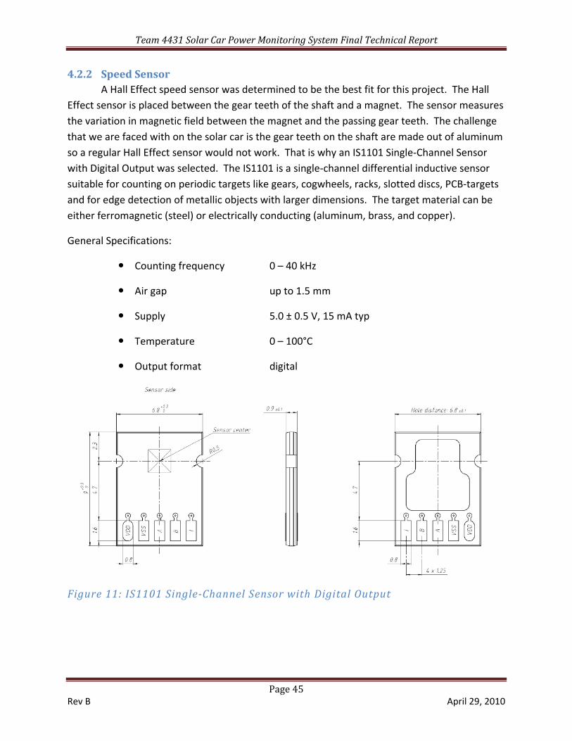
4.2.2 Speed Sensor A Hall Effect speed sensor was determined to be the best fit for this project. The Hall Effect sensor is placed between the gear teeth of the shaft and a magnet. The sensor measures the variation in magnetic field between the magnet and the passing gear teeth. The challenge that we are faced with on the solar car is the gear teeth on the shaft are made out of aluminum so a regular Hall Effect sensor would not work. That is why an IS1101 Single‐Channel Sensor with Digital Output was selected. The IS1101 is a single‐channel differential inductive sensor suitable for counting on periodic targets like gears, cogwheels, racks, slotted discs, PCB‐targets and for edge detection of metallic objects with larger dimensions. The target material can be either ferromagnetic (steel) or electrically conducting (aluminum, brass, and copper).
General Specifications:
Counting frequency 0 – 40 kHz
Air gap up to 1.5 mm
Supply 5.0 ± 0.5 V, 15 mA typ
Temperature 0 – 100°C
Output format digital
Figure 11: IS1101 SingleChannel Sensor with Digital Output
Team 4431 Solar Car Power Monitoring System Final Technical Report
Page 46 Rev B April 29, 2010
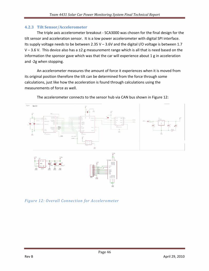
4.2.3 Tilt Sensor/Accelerometer The triple axis accelerometer breakout ‐ SCA3000 was chosen for the final design for the
tilt sensor and acceleration sensor. It is a low power accelerometer with digital SPI interface. Its supply voltage needs to be between 2.35 V – 3.6V and the digital I/O voltage is between 1.7 V – 3.6 V. This device also has a ±2 g measurement range which is all that is need based on the information the sponsor gave which was that the car will experience about 1 g in acceleration and ‐2g when stopping.
An accelerometer measures the amount of force it experiences when it is moved from its original position therefore the tilt can be determined from the force through some calculations, just like how the acceleration is found through calculations using the measurements of force as well.
The accelerometer connects to the sensor hub via CAN bus shown in Figure 12:
Figure 12: Overall Connection for Accelerometer
Team 4431 Solar Car Power Monitoring System Final Technical Report
Page 47 Rev B April 29, 2010
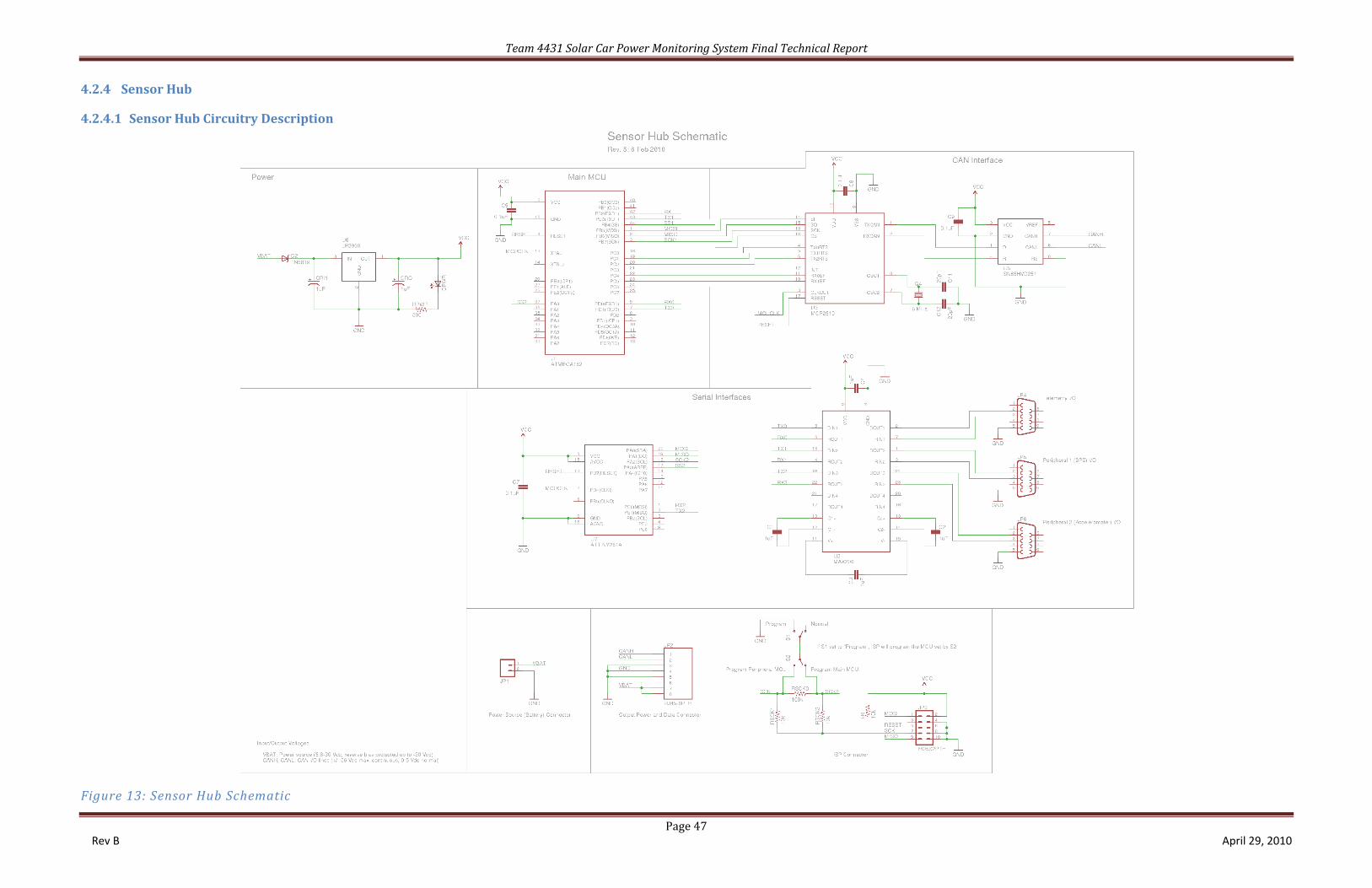
4.2.4 Sensor Hub
4.2.4.1 Sensor Hub Circuitry Description
Figure 13: Sensor Hub Schematic
Team 4431 Solar Car Power Monitoring System Final Technical Report
Page 48 Rev B April 29, 2010
4.2.4.1.1 I/O Ratings
Table 20: Input/Output Ratings VBAT Power source ( V305.8− , reverse bias protected up to ‐30 V)
CANH, CANL CAN bus communications lines ( V50 − nominal, V± 36 maximum continuous)
Serial lines RS‐232 levels ( V± 30 maximum)
4.2.4.1.2 Overview The sensor hub provides an interface to the various sensors and aggregates their data. This aggregated data is then sent out to the ground station computer in a serial stream. The serial stream must efficiently pack data into the fewest bits possible to be compatible with slow serial baud rates (such as 9600 Baud/s) that may be required by the telemetry hardware.
For wired telemetry, the sensor hub may be directly connected to the ground station computer via a serial cable. For wireless telemetry, a radio modem may be connected to the sensor hub and another radio modem connected to the ground station computer. These modems act to ”tunnel” serial data between the sensor hub and ground station computer nodes.
The sensor hub has the ability to interface with one RS‐232 serial device (e.g. the BPS) and up to 13 CAN bus‐equipped devices (this device limitation is due to the number of physical connectors). The sensor hub will also provide power to all sensors designed or supplied by the project.
4.2.4.1.3 Connectors The power source connector ( 1JP ) supplies power to the sensor hub (and to external
sensors). The connector is a Deans Ultra male plug, a connector that is compatible with many batteries used for R/C applications.
The output power and data connector ( 2JP ) supplies unregulated power to external
custom sensors and also provides access to the two CAN communication lines (CANH and CANL). The connector is an RJ‐45 connector as the intended cabling is CAT5 UTP patch cable.
The cabling was chosen to accommodate the suggested Ω120 characteristic impedance of the CAN bus lines and as the twisted‐pair design of CAT5 cabling maximizes the noise‐canceling capability of the CAN bus’ differential signal communications. CAT5 UTP cable is readily available due to its use as Ethernet patch cabling.
The ISP connector ( 3JP ) allows for in‐system programming of the ATmega162
microcontroller (MCU).
Team 4431 Solar Car Power Monitoring System Final Technical Report
Page 49 Rev B April 29, 2010
The two RS‐232 serial lines (telemetry I/O and peripheral I/O) use DB‐9 connectors ( 3JP
and 4JP ) as these are the most common connectors used for RS‐232 communications and are
able to interface with the current telemetry and peripheral hardware.
4.2.4.1.4 Digital Circuitry
4.2.4.1.4.1 Microcontroller The sensor hub microcontroller, 1U , is tasked with aggregating data from various
sensors and outputting this aggregated data as telemetry. The telemetry is packed efficiently so that a minimum number of bits are needed for the data. This is important when using slower telemetry devices, such as a 9600 Baud/s radio modem, so that information can be sent
in a timely manner and without backlog. The 1U is an AVR ATmega162 with enough processing
power and memory storage to accomplish this task (and more, if needed). Additionally, the MCU features dual UARTs (universal asynchronous receiver/transmitters). These UARTs are hardware features that allow for easy dual full‐duplex serial communications. This allows for simultaneous communications between the sensor hub and BPS and the sensor hub and ground station computer (via telemetry).
4.2.4.1.4.2 Serial Interface Two RS‐232 serial interfaces exist: one for telemetry communications and one for peripheral sensor communications. Both of these interfaces are full‐duplex, meaning information can be sent and received simultaneously. Although this feature will most likely not be used with the current system setup, the ability to perform full‐duplex serial communications is important to avoid limiting future applications of the sensor hub.
While the 1U microcontroller operates at the V50 − level, the RS‐232 line operates at
V±12 . In order to interface these two voltages levels, the 2U TRS232E RS‐232 driver/receiver
is used. The TRS232E supports dual full‐duplex communications and is powered by the V5 supply. Charge pumps are used to generate the needed RS‐232 voltages levels.
4.2.4.1.4.3 CAN Bus Interface Much of the sensor data is retrieved from the CAN bus (which supports up to 13 sensors/devices).
8U is the CAN controller that takes the MCU data and forms a proper CAN message,
which is sent to the CAN transceiver ( 10U ). The CAN transceiver interfaces with the physical
CAN bus and converts the CAN message into the proper voltage signals to send over the bus. The process works in reverse for CAN messages being received.
Team 4431 Solar Car Power Monitoring System Final Technical Report
Page 50 Rev B April 29, 2010
4.2.5 Communications Hub The schematic for the communications hub is shown in Figure 14:
Figure 14: Communication Hub Schematic
4.2.5.1 Communications Hub Description The purpose of the communications hub is to limit the connectors to external sensors on the sensor hub by providing an auxiliary dedicated connector board for the sensor power and CAN communications cabling. This makes it easy to update the system to handle additional sensors on the CAN bus (each of which requires their own connector to interface with the bus): simply daisy‐chain another communications hub board for additional connections. The communications hub can also limit the amount of cabling used to connect the sensor hub to the
Team 4431 Solar Car Power Monitoring System Final Technical Report
Page 51 Rev B April 29, 2010
sensors. For example, if half of the sensors are physically near the sensor hub and the other half are on the other side of the vehicle, one communications hub could be used to handle the near sensors and another the far sensors. The far sensors’ cabling would only have to reach the far communications hub (which is close to these far sensors) and a single cable from this communications hub could be run to the other hub, which connects to the sensor hub, rather than having all of the far sensor cables running back to the sensor hub.
The communications hub is a simple board consisting of eight RJ‐45 connectors with all pin 1s connected together, all pin 2s connected together, etc., up to the fourth pin. Pin 1 is VBAT (battery positive voltage); pin 2 is GND (system ground), pin 3 is CANH (CAN bus high line); and pin 4 is CANL (CAN bus low line). The VBAT and GND wires supply power to custom sensors and the CANH and CANL lines provide a CAN bus connection used by the majority of the sensors (even to those not acquiring power from this cabling).
As previously mentioned, a communications hub board may be daisy‐chained with another, expanding the number of sensors that can communicate over the CAN bus. As the design is required to support 13 devices on the CAN bus, a total of two communications hubs will be used (daisy‐chained together) to provide all 13 connectors.
Team 4431 Solar Car Power Monitoring System Final Technical Report
Page 52 Rev B April 29, 2010
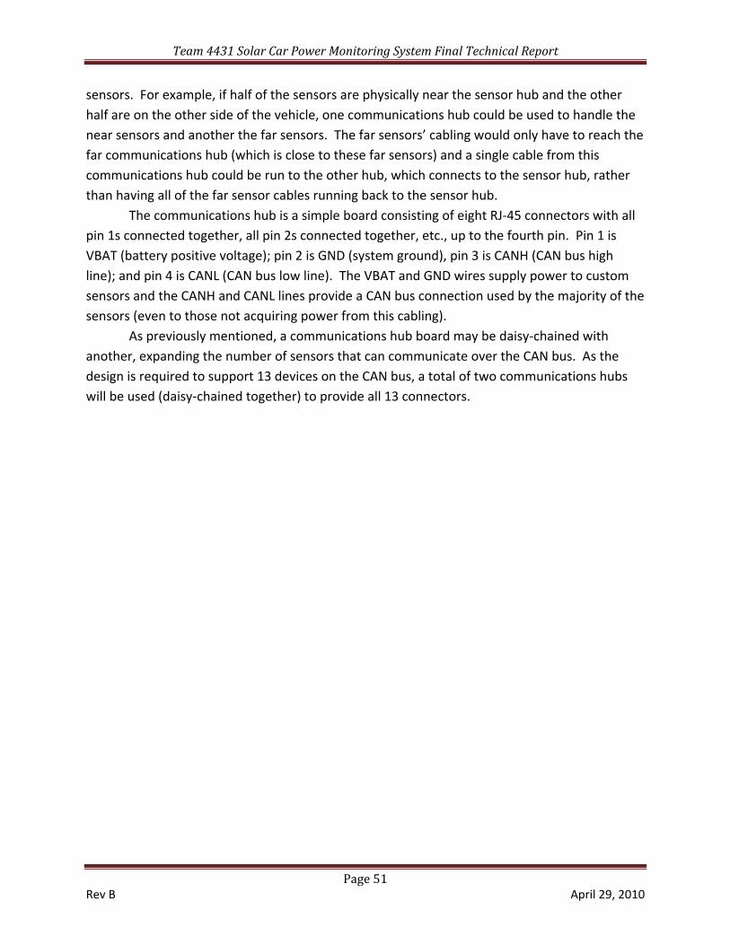
4.3 Telemetry The telemetry component selected for the final design is the XStream OEM RF Module.
According to the datasheet, these devices are capable of an outdoor line of sight range of 7 miles which exceeds our FR for the telemetry range. This device has a frequency of 900MHz and receiver sensitivity of ‐110 dBm. The only concern we have is that the throughput data rate of 9,600 bps may not be enough for all of the data we have to transmit between the car and compute over the telemetry system.
The sensor hub and the computer will interface with the XStream Modules as show in the following figures. In Figure 15 the sensor hub is host A and the computer is host B because host A is on the transmission side and host B is on the receiver side. Figure 16 shows the cables that will be used to make the connections shown in Figure 15.
Figure 15: System Block Diagram for Telemetry
Figure 16: Module Assembly from the Product Manual
Team 4431 Solar Car Power Monitoring System Final Technical Report
Page 53 Rev B April 29, 2010
4.4 Software
4.4.1 Capture and Visualization Software Description
Figure 17: Visualization Software
4.4.1.1 Overview The capture and visualization software is used to capture telemetry sent out from the sensor hub and to plot the captured data in real‐time or after a data capture. The software is run on the ground station computer (GSC) and is written using LabView. The LabView environment was chosen for its ease‐of‐use in creating graphical user interfaces (GUIs) and for its ability to easily interface with external devices.
4.4.1.2 Capture The software captures a telemetry stream sent from the sensor hub and parses this stream into measurements from different sensors (e.g. voltage, current, tilt readings). The data stream is accessed from a software serial device. Any device with a software device driver replicating a serial port (e.g. a USB‐to‐serial adaptor) may be used to send the telemetry information to the device. The current setup interfaces a radio modem with RS‐232 output to the GSC via a USB‐to‐serial adapter.
Once the telemetry data stream is parsed, the data is saved to text tab delimited file. A tab delimited file separates fields (columns) with a "tab" delimiter and separates entries (rows) by newlines. Each sensor data record is placed in its own field and each complete data query (i.e. data from all sensors taken at one time) is placed in its own entry. This text format was chosen because tab delimited files can be read by many common applications (e.g. Notepad,
Team 4431 Solar Car Power Monitoring System Final Technical Report
Page 54 Rev B April 29, 2010
Excel) and the data can be stored in a human readable way. This helps to ensure the data will be able to be accessed in the future.
4.4.1.3 Visualization Data is plotted on a configurable canvas. All data can be displayed or the display can be limited to the last n seconds of data (where n is an arbitrary real number) if the displayed data is from a real‐time source.
The canvas consists of one or more plots, which can be added or removed from the user interface (UI). Each plot can display data from any sensor or any combination of sensors, all configurable through LabView utilities. The plots can be re‐arranged on the canvas via the up‐arrow and down‐arrow buttons. For data from stored (non‐real‐time sources), the plots will have the ability to zoom in on different portions of the data.
Team 4431 Solar Car Power Monitoring System Final Technical Report
Page 55 Rev B April 29, 2010
4.5 Mechanical
4.5.1 Wheel Alignment Tool The team chose a digital alignment tool out of the two designs that were being considered. The final design is as shown in Figure 18:
Figure 18: Final Digital Alignment Tool Design
4.5.1.1 The Arms The tool has three arms which are used to attach to the tires of any car
4.5.1.1.1 Material The Aluminum is 6063‐T53 metal. This metal was the cheapest metal we could find to fit
the design hoped for, which is square tubing 1/2’’ thick. Although it was the cheapest, it was fine for the amount of work we required. The metal has yield strength of 16,000 psi. The factor of safety was in the number of hundreds due to the only weight being the digital protractor. To find this safety factor, the following equation was used:
Equation 18 Safety factor due to static loading
N= safety factor S=material strength A=area of loading P=loading force
Team 4431 Solar Car Power Monitoring System Final Technical Report
Page 56 Rev B April 29, 2010
4.5.1.1.2 Design The two bottom arms consist of foot long aluminum square tubing having 10 holes for
configuration and a bottom hole to attach to the digital tool. The holes are in place every ¾’’. This number was chosen based on the wheel sizes of trailer tires that the solar car team was using. The digital protractor was going to be most aesthetic while placed in the center of the tire. Thus the arms should be approximately the radius of the tire. Using that as a reference the arms were punched along the most common radii of trailer tires. The holes were a size of 3/8’’ to use a hand screw of such a diameter to attach to the tires. The holes were tapped for the hand screw to ensure most accurate results. The final bottom hole was selected to be ¼’’ diameter to be used with the other hand screws which attached it to the digital protractor. Below is a schematic of this arm:
Figure 19 Wheel alignment bottom arms
Team 4431 Solar Car Power Monitoring System Final Technical Report
Page 57 Rev B April 29, 2010
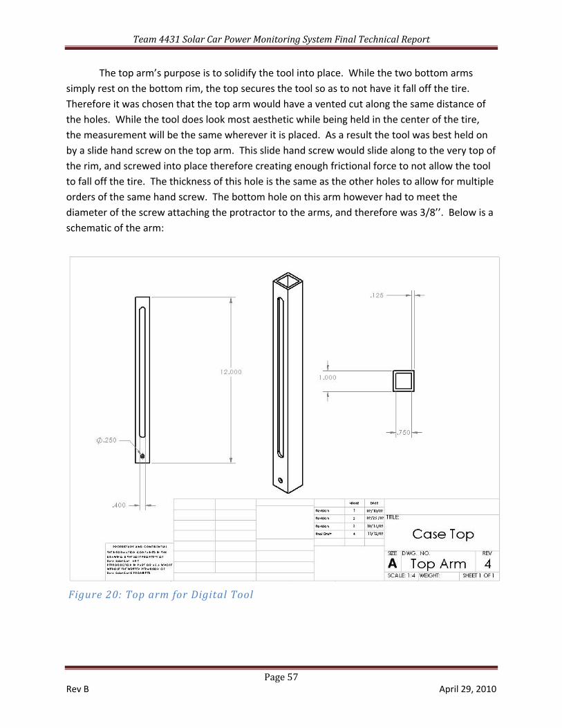
The top arm’s purpose is to solidify the tool into place. While the two bottom arms simply rest on the bottom rim, the top secures the tool so as to not have it fall off the tire. Therefore it was chosen that the top arm would have a vented cut along the same distance of the holes. While the tool does look most aesthetic while being held in the center of the tire, the measurement will be the same wherever it is placed. As a result the tool was best held on by a slide hand screw on the top arm. This slide hand screw would slide along to the very top of the rim, and screwed into place therefore creating enough frictional force to not allow the tool to fall off the tire. The thickness of this hole is the same as the other holes to allow for multiple orders of the same hand screw. The bottom hole on this arm however had to meet the diameter of the screw attaching the protractor to the arms, and therefore was 3/8’’. Below is a schematic of the arm:
Figure 20: Top arm for Digital Tool
Team 4431 Solar Car Power Monitoring System Final Technical Report
Page 58 Rev B April 29, 2010
4.5.1.2 Hand Screws
The hand screws were selected based on appropriate compatible sizing.
4.5.1.2.1 10x1.5 screws There are three 10x1.5 hand screws used on the tool. These three screws are used to
attach the tool to the tire. The selection was based on the side of the threads. Using a thread count smaller than 1.5mm allowed for 4 of the threads to be connected to the tire rim of the current car. While only one thread is required to create the frictional force required a higher safety factor was good to have based on the fact that smaller tire rims could be used in the future. The equation used for frictional force is below:
Equation 19 Frictional Force
Ff = frictional force
This screw also worked due to the length of the screw. It was one of the few hand screws we could find that was at least 2 inches in length. This length is critical because the tool must stand a small distance away from the center of the tire where certain rims can obstruct the ability for the tool to hook onto the rim.
4.5.1.2.2 6x1mm screws There are two 6x1 hand screws used in this tool. These secure the arms in place to the
digital protractor during use of the tool. They screw into the beam threads which have an open end. This open end allows for slight bending, which then creates a friction force against the arms. This force temporarily locks the arms in place during use and during transport. The screw was one of the few smaller screws that were a size of 1.5 inches in length, which was required.
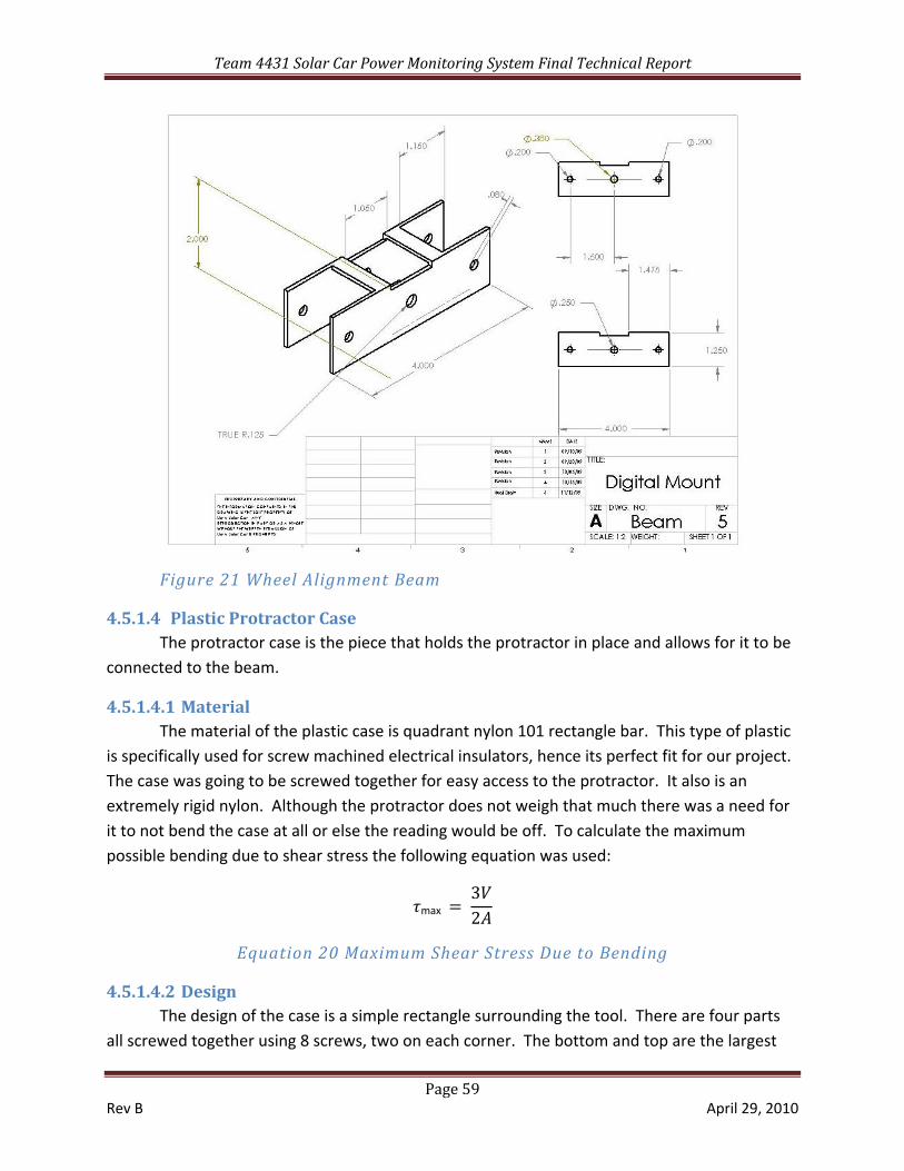
4.5.1.3 The Beam The beam is the name used for the piece connecting the arms to the protractor. The
beam is made up of steel square tubing with three cuts in it. The first cut is a square cut in the top center where the middle arm goes into place. This is in the direct center of the beam and is only 1.005 inches in width to allow for a very slight clearance for the top arm. The other two cuts are through both the top and bottom on the ends of the bar. This allows for a slight bending which pinches the two bottom arms of the tool. To get this sort of bend the cut needed to be 1.25 inches in thickness.
Team 4431 Solar Car Power Monitoring System Final Technical Report
Page 59 Rev B April 29, 2010
Figure 21 Wheel Alignment Beam
4.5.1.4 Plastic Protractor Case The protractor case is the piece that holds the protractor in place and allows for it to be
connected to the beam.
4.5.1.4.1 Material The material of the plastic case is quadrant nylon 101 rectangle bar. This type of plastic
is specifically used for screw machined electrical insulators, hence its perfect fit for our project. The case was going to be screwed together for easy access to the protractor. It also is an extremely rigid nylon. Although the protractor does not weigh that much there was a need for it to not bend the case at all or else the reading would be off. To calculate the maximum possible bending due to shear stress the following equation was used:
max 32
Equation 20 Maximum Shear Stress Due to Bending
4.5.1.4.2 Design The design of the case is a simple rectangle surrounding the tool. There are four parts
all screwed together using 8 screws, two on each corner. The bottom and top are the largest
Team 4431 Solar Car Power Monitoring System Final Technical Report
Page 60 Rev B April 29, 2010
pieces, overlapping the sides. The screws therefore go through the top and bottom to the sides. These parts extend only the thickness of the plastic to ensure a tight fit of the protractor. To ensure the protractor does not move these parts have an extruded cut in the exact shape of the digital protractor at a thickness of 1/10 of an inch on both the bottom and top.
4.5.1.5 Digital Protractor The digital protractor used is the SPI Digital Protractor angle measurement tool. This
tool had multiple characteristics which made it perfect for the project.
4.5.1.5.1 Capabilities The protractor has two modes, absolute and zero. The absolute goes off of a previously
configured point which is considered absolute 0 degrees, i.e. horizontal. This is used to find the camber of the tire. While the tool is on the car the tool would measure how big the angle between absolute horizontal and the current angle. The zero function allows for the ability to measure a certain degrees relative to another. For perfect toe, the tires in the same plane need to be parallel. Therefore if the tires do not have the same angle when the tool is measuring the angle off of the vertical axis, one knows that something is wrong.
4.5.1.5.2 External Characteristics The protractor has numerous external characteristics which make it work for the tool also. The tool can work in temperature required by the solar team without any negative effects. The car is made in Tucson, so there are quite a range of temperatures the tool will experience. The tool has easy battery replacement which allowed for the batteries to be replaced without taking apart the entire wheel alignment tool. The size of the tool was perfect also, being only 6 inches long, 1 inch tall, and wide.
Team 4431 Solar Car Power Monitoring System Final Technical Report
Page 61 Rev B April 29, 2010
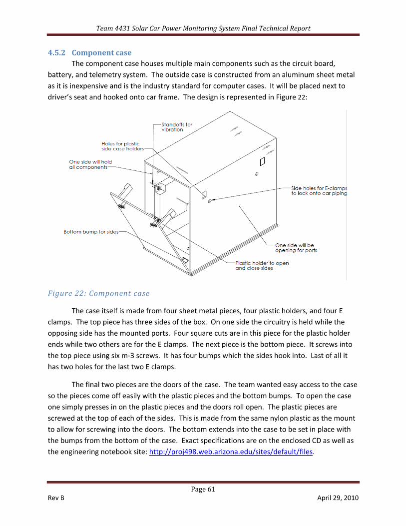
4.5.2 Component case The component case houses multiple main components such as the circuit board, battery, and telemetry system. The outside case is constructed from an aluminum sheet metal as it is inexpensive and is the industry standard for computer cases. It will be placed next to driver’s seat and hooked onto car frame. The design is represented in Figure 22:
Figure 22: Component case
The case itself is made from four sheet metal pieces, four plastic holders, and four E clamps. The top piece has three sides of the box. On one side the circuitry is held while the opposing side has the mounted ports. Four square cuts are in this piece for the plastic holder ends while two others are for the E clamps. The next piece is the bottom piece. It screws into the top piece using six m‐3 screws. It has four bumps which the sides hook into. Last of all it has two holes for the last two E clamps.
The final two pieces are the doors of the case. The team wanted easy access to the case so the pieces come off easily with the plastic pieces and the bottom bumps. To open the case one simply presses in on the plastic pieces and the doors roll open. The plastic pieces are screwed at the top of each of the sides. This is made from the same nylon plastic as the mount to allow for screwing into the doors. The bottom extends into the case to be set in place with the bumps from the bottom of the case. Exact specifications are on the enclosed CD as well as the engineering notebook site: http://proj498.web.arizona.edu/sites/default/files.
Team 4431 Solar Car Power Monitoring System Final Technical Report
Page 62 Rev B April 29, 2010
4.6 Analysis Mechanical analysis was done to the car so that the performance of it can be optimized. The team was given the task to find the optimal gear ratio for the solar car. This analysis also justifies the use of a wheel alignment tool. This can be done using Equation 21:
RPMP
GearRatio engine
*2Π=
Equation 21: Gear Ratio
Where RPM is the revolutions per minute for the engine therefore engineP needs to be
calculated. engineP is the driven wheel power.. To calculate engineP
Equation 22 is used:
VFDFP massrollingengine *)( ++=
Equation 22: Driven Wheel Power, P engine
Where rollingF is the rolling resistance created from the tire contact with the road. It is also
called tire drag. To determine rollingF:
gmRF xrolling **=
Equation 23: F rolling
xR is the rolling resistance coefficient which is approximately 0.03 for a typical passenger car tire and 0.005 for racecar tires. The weight of the car (m*g) is the mass of the car times gravity.
D in equation 19 is the aerodynamic drag of a vehicle. To determine it Equation 24 is used:
2****5.0 VACD Dρ=
Equation 24: Aerodynamic Drag
ρ is the local air density
DC is the drag coefficient which is determined by using a coastdown test (later described)
Team 4431 Solar Car Power Monitoring System Final Technical Report
Page 63 Rev B April 29, 2010
A is the frontal area of the vehicle.
V is the vehicle velocity.
massF is the amount of force available to accelerate the car .It is defined by Equation 25.
rolling
massmass r
TF =
Equation 25: Force
rollingr is the rolling radius of the tires (outside radius).
massTis the amount of torque available to accelerate the car. It is calculated by using Equation
26.
rollinglongfmass rGMmT ***=
Equation 26: Torque
longGis the longitudinal acceleration of the system measured by the data logging system
(accelerometer)
fM is a factor that takes into account driveline rotational inertias and the mass factor.
MMMM r
f+
=
Equation 27: Mass Factor
M is the translational mass of the vehicle (m/g)
rM is the equivalent rotational mass
If the wheel are misaligned then the rolling resistance increases making the driven wheel power decrease (because the rolling resistance is in the opposite direction with respect to the vehicle’s
Team 4431 Solar Car Power Monitoring System Final Technical Report
Page 64 Rev B April 29, 2010
moving direction). A chart of how misalignment and different tire pressures can increase the rolling resistance coefficient is shown in Figure 23.
Figure 23: Rolling Resistance
The coastdown test
The coastdown test is done by driving the car on a straight asphalt road as smooth as possible (so that only aerodynamic drag slows the car down). After a certain speed car is shifted into neutral and allowed to coast down to a lower predetermined speed. This test is used to determine the drag coefficient by using Equation 28.
AVam
C longD ***5.0
*2ρ
=
Equation 28: Drag Coefficient
longais the longitudinal acceleration (deceleration in this case) of the car. It is easily
measured by recording the velocity of the car with respect to time during the test.
In Figure 24 a coastdown test performed for a Dodge Viper GTS‐R chart of speed versus time is shown.
Team 4431 Solar Car Power Monitoring System Final Technical Report
Page 65 Rev B April 29, 2010
Figure 24: Coastdown Test
Team 4431 Solar Car Power Monitoring System Final Technical Report
Page 66 Rev B April 29, 2010
4.7 FMEA Component Function Failure Consequence Cause Mitigation
V/I Sensor Measures voltage and current on a conductor
Line voltage spike > 0.5 V above line voltage at input
IC is fried and current sensing will not work
Voltage spike The resistance of the solid‐state relays between the line and amplifier inputs will protect the inputs from voltages
across Rshunt due to currents of up to 3.4 kA
Line‐level voltage drops below ~4 V
Current sensing will not work The floating ground regulator is referenced at ground, limiting
FGND to ~1V
Reference floating ground regulator to ‐5 V, allowing operation with line voltages down to 0 V
Moisture contamination Moisture could cause electronics to
fail Moisture Seal electronics from environments using encapsulate
Data output connection fails Sensor fails to transmit data Solder failure Ensure adequate solder adhesion
Wire failure Ensure wire routing is clear of obstructions
Voltage regulator The sensor will not be supplied with
power and will fail to work
Battery is plugged in backward Use polarized battery connectors and use a diode to
protect the voltage regulator from negative input voltages
High‐voltage power source connected
The voltage regulator is chosen to operate under potentially high voltages (i.e. receiving input voltage up to
30 V)
Speed Sensor Sense vehicle speed Air Gap
Sensor will fail to sense speed Air Gap too large Set Air Gap correctly using hardware that rigidly holds
sensor in proper orientation
Speed sensing will be inaccurate Air Gap too large/small Set Air Gap correctly using hardware that rigidly holds
sensor in proper orientation
Speed sensor will contact gear causing damage to sensor and/or
gear Air Gap too small
Set Air Gap correctly using hardware that rigidly holds sensor in proper orientation
Tilt Sensor Sense solar array tilt
Voltage Drop Sensor will fail to sense tilt Solder failure ensure adequate solder adhesion
Wire failure ensure wire routing is clear of obstructions
Voltage regulator failure Sensor electronics fried; tilt sensing
will no longer work Voltage spike
The voltage regulator is chosen to operate under potentially high voltages (i.e. receiving input voltage up to
30 V). The diode in front of the regulator will fail at sufficiently high voltages, protecting the rest of the
circuitry.
Telemetry
Transmit vehicle data
Out of range Data transmitted while out of range
is lost Exceeding range capability of
radios Ensure radio range is longer than required
Interference Data transmitted while interference is present may be lost or scrambled
Ensure operability of radios in secluded environment
Ask testing facility about other frequencies in operation, utilize other channels when available
Receive vehicle data Out of range
Data received while out of range is lost
Exceeding range capability of radios
Ensure radio range is longer than required
Interference Data received while interference is present may be lost or scrambled
Ensure operability of radios in secluded environment
Ask testing facility about other frequencies in operation, utilize other channels when available
Team 4431 Solar Car Power Monitoring System Final Technical Report
Page 67 Rev B April 29, 2010
FMEA Continued
Component Function Failure Consequence Cause Mitigation
Rolling Resistance increased causing more mechanical drag
Incorrect wheel alignment settings
Calibrate fixture prior to using
Incorrect use of fixture Rolling Resistance increased causing more mechanical drag
Incorrect wheel alignment settings
Develop instruction manual or how to guide to ensure proper use
System Wiring Carry signals between
devices
Wire chafing Wires can short to ground
Improper routing and protection
Properly route wires away from sharp objects
Wires can short to power Improper routing and
protection Properly route wires away from sharp objects
Interference Wires can pickup interference
causing incorrect values Improper routing and shielding Properly route wires away from main power supplies
Sensor Hub Collect signals from sensors
Voltage Drop Sensor hub fails to collect data and
send to telemetry Solder failure Ensure adequate solder adhesion
Wire failure Ensure wire routing is clear of obstructions
Voltage regulator failure Sensor hub electronics fried and
hub no longer works Voltage spike
The voltage regulator is chosen to operate under potentially high voltages (i.e. receiving input voltage up to
30 V). The diode in front of the regulator will fail at sufficiently high voltages, protecting the rest of the
circuitry.
Software Display data on ground
station computer
Failure to read data Data is not read and data is lost Incorrect software configurationTest individual sensor streams with known levels to
ensure proper read in
Incorrect data parsing Data is recorded but not usable Incorrect setting in software Test groups of sensor streams with known levels to ensure
proper parsing
Failure to display data Data is recorded but not usable Incorrect setting in software Test groups of sensor streams with known levels to ensure
proper display
Calculations Analyze vehicle data
Incorrect computations Invalid data
Improper use of equations Validate each equation with other experts in the field to
ensure proper calculations
Error in computations Validate each computation with mathematical software
and/or other experts in the field to ensure proper calculations
Incorrect measurements Incorrect computations
Incorrect measurement technique
Measure each attribute more than once
Incorrect recording of measurements
Record measurements with more than one person to validate each recorded measurement
Team 4431 Solar Car Power Monitoring System Final Technical Report
Page 68 Rev B April 29, 2010
4.8 Risk Risks have been identified throughout the project and tracked for resolution and mitigation. Risk register is used to identify risks to the project.
Table 21: Risk Register
No. Risk Likelihood Severity Risk Factor
Mitigation
1 V/I Sensor fails to operate as designed
0.5 0.9 0.45 Extensive analysis and research, review with industry experts
2 Sensor Accuracy not as designed
0.5 0.5 0.25 Adjustments with component replacement or software calibration
3 Telemetry does not perform over range
0.2 0.4 0.08 Evaluate telemetry performance, purchase different radios?
0.3 0.8 0.24 Investigate alternative sensing methods (low/high side current)
6 MPG calculation not available
0.2 0.5 0.15 Cannot optimize setup for race goal, utilize Shell Eco data to calculate
7 Gear ratio optimization
0.1 0.9 0.09 Leverage experts to assist calculation to ensure optimized ratios
8 Weight 0.5 0.2 0.01 Ensure lightweight components are utilized when possible
9 Cost 0.5 0.6 0.30 Only purchase necessary components. Introduces risk with schedule if replacement contingency parts are not available
Team 4431 Solar Car Power Monitoring System Final Technical Report
Page 69 Rev B April 29, 2010
Figure 25: Risk Plot
1
2
3 4
5
6
7
8
9
0
0.1
0.2
0.3
0.4
0.5
0.6
0.7
0.8
0.9
1
0 0.1 0.2 0.3 0.4 0.5 0.6 0.7 0.8 0.9 1
Potential Severity of Occurrence
Relative Likelihood of Occurrence
Team 4431 Solar Car Power Monitoring System Final Technical Report
Page 70 Rev B April 29, 2010
5 System Build
5.1 V/I Sensor
5.1.1 Construction The V/I Sensor printed circuit board (PCB) was designed to take into account the noise‐sensitive, high‐precision analog circuitry that the sensor relies upon, as well as the potentially large differences in subsystem voltages. This design was then refined over several iterations in order to produce a high‐performance board design with the parts and part packages available. The physical parts to be placed on the board were then overlaid on a 1:1 printout of the PCB to ensure valid component footprints. The PCB was then sent to be manufactured by a third‐party company, components were placed on the board, and the firmware was loaded onto the sensor. Calibration was then performed on the sensor by applying known voltages across the device, measuring the current through the device with a high‐precision multi‐meter, and modifying the firmware’s calibration data accordingly.
5.1.2 Testing In order to test the V/I Sensor, different known voltages and current were fed into the sensor to simulate the currents and voltages found within the Solar Car subsystems that were to be measured by the V/I Sensor. Firmware modifications were made based upon the test data.
5.2 Speed Sensor
5.2.1 Construction The speed sensor is an off the shelf component to be integrated into our system. This sensor was evaluated and determined to be compatible with our system however due to budget and time constraints the parts have not been procured. This part comes from Switzerland and has a lead time of 2 months minimum. Specifications and interconnects have been provided so this sensor can be integrated into the vehicle at a later time, if desired.
5.2.2 Testing Testing of the speed sensor has not been physically completed, but has been validated by analysis. The IS1101 speed sensor has a digital output that can easily be integrated into the sensor hub.
5.3 Tilt Sensor/Accelerometer
5.3.1 Construction The accelerometer is an off the shelf component to be integrated into our system. This sensor was evaluated and determined to be compatible with our system.
Team 4431 Solar Car Power Monitoring System Final Technical Report
Page 71 Rev B April 29, 2010
5.3.2 Testing The accelerometer was tested and calibrated per the manufacturer’s recommendations.
5.4 Sensor Hub
5.4.1 Construction The Sensor Hub printed circuit board (PCB) was designed to take into account the noise‐sensitive, high‐precision analog circuitry that the sensor relies upon, as well as the potentially large differences in subsystem voltages. This design was then refined over several iterations in order to produce a high‐performance board design with the parts and part packages available. The physical parts to be placed on the board were then overlaid on a 1:1 printout of the PCB to ensure valid component footprints. The PCB was then sent to be manufactured by a third‐party company and components were placed on the board.
5.4.2 Testing The Sensor Hub was tested by connecting the system’s sensors to the Sensor Hub and ensuring that data was properly aggregated and outputted to the telemetry stream. The data sent out over the telemetry stream was then manually verified.
5.5 Communications Hub
5.5.1 Construction The Communications Hub printed circuit board (PCB) was designed to take into account the noise‐sensitive, high‐precision analog circuitry that the sensor relies upon, as well as the potentially large differences in subsystem voltages. This design was then refined over several iterations in order to produce a high‐performance board design with the parts and part packages available. The physical parts to be placed on the board were then overlaid on a 1:1 printout of the PCB to ensure valid component footprints. The PCB was then sent to be manufactured by a third‐party company and components were placed on the board.
5.5.2 Testing The Communications Hub was tested by inserting a CAT5e cable, with RJ45 connector on one end and exposed wire on the other, into each RJ45 socket on the board. Each input was tested with a multi‐meter to ensure proper conductivity to the appropriate conductor on the board.
Team 4431 Solar Car Power Monitoring System Final Technical Report
Page 72 Rev B April 29, 2010
5.6 Telemetry
5.6.1 Construction The telemetry is an off the shelf component to be utilized by our system. The telemetry radios are already owner by the UA Solar Racing Team and deemed sufficient to support our system.
5.6.2 Testing The only testing required for the telemetry was range and data capability. Per specification, the range of these units far exceeds 1.5 miles and the data rate supports our needs.
5.7 LabView Software
5.7.1 Construction The LabView software was created with multiple inputs and outputs to allow for a broad spectrum of capabilities. Input options include file read in, specific sensor (channel) read in and data acquisition read in. File read in allows the user to read in saved files for many purposes including files with known values to ensure readout accuracy, as well as reviewing saved files from previous data acquisition sessions. Channel specific read in allows a specific channel to be viewed isolated from other values for individual troubleshooting. Data acquisition read in is the live collection of data method over USB, serial or other interface (including telemetry). All input options include the ability to record the raw data prior to processing to ensure data integrity before manipulation within the program. Output options include on‐screen display of all data, selected data as well as output to file.
Processing of the data is completed in steps. First the data is acquired and strings are selected within the data based on device type and device id parameters. The data is sorted into an array and stored in memory. The visualization process selects data form the array, indexes the data and outputs to a waveform graph based on device type and id’s selected in the viewing window.
5.7.2 Testing To test the functionality of the capture and display software, a series of tests were created and implemented. Initially an Excel file was created with known values for each sensor. The Excel file contains columns of information related to device type, device id, and sensed value. Each of these numeric inputs is fed through a series of equations to translate the numeric inputs into binary strings. The binary strings are fed through the LabView program and read out on the visualization screen as well as written to a tab delimited file. The values received on the final processing end were compared to the read in values to ensure accuracy.
Team 4431 Solar Car Power Monitoring System Final Technical Report
Page 73 Rev B April 29, 2010
Once known values were evaluated, random values generated from the Excel file were used to ensure parsing was accurate. These files were recorded before and after parsing and compared for accuracy.
Finally, actual data from sensors was sent across the telemetry through serial interface and read into the LabView program. Known values were used across the V/I sensor and validated in the outputs of the LabView program.
5.8 Mechanical
5.8.1 Wheel Alignment Tool The basic design of the wheel alignment tool is a digital protractor held within a plastic casing attached to a beam piece which is then connected to three arms. The three arms would lock onto a tire rim allowing for the protractor to measure the angle of the wheel. This angle would be used in the toe and camber wheel alignment settings.
5.8.1.1 The Arms The tool has three arms which are used to attach to the tires of any car
5.8.1.1.1 Construction The arm material is 6063‐T53 Aluminum. The initial cut to shorten the metal from its
original length was made using a large scale band saw. The band saw was set to cut at a very slow rate in addition to a constant stream of lubrication applied to the saw blade to ensure material property integrity. Once the piece was cut into the three one‐foot sections the holes were cut using a vertical drill press. Using both motor oil and a slow rate of cutting ensured the metal properties were kept intact. Following the de‐burring process of each of the holes a screw tap was used to make the screw threads for the hand screws to securely pass through. The taps followed the charts given by ISO 724:1993 standards for 75% thread. The top arms have a groove for the hand screw to slide up and down along. This groove was done using an end mill the same width as the grove length. To ensure the metal integrity the piece was only milled at fifteen thousandths of an inch at a time along the use of motor oil as lubrication.
5.8.1.2 The Beam The beam is the name used for the piece connecting the arms to the protractor.
5.8.1.2.1 Construction The beam is made up of steel square tubing with three cuts in it. The first cut is a square
cut in the top center where the middle arm goes into place. This cut was made using an end mill in perpendicular cuts. To ensure material properties were kept as they were originally the cuts were only ten thousands at a time with the use of motor oil. The other two cuts were made using a mill process cutting out the square to the thousandth of an inch until the square
Team 4431 Solar Car Power Monitoring System Final Technical Report
Page 74 Rev B April 29, 2010
was completely dislocated. De‐burring the edges followed the mill work. Finally the center hole was cut using a vertical drill press within a vise.
5.8.1.3 Plastic Protractor Case The protractor case is the piece that holds the protractor in place and allows for it to be
connected to the beam.
5.8.1.3.1 Construction The material of the plastic case is quadrant nylon 101, rectangular bar. This type of
plastic is specifically used for screw machined electrical insulators, hence its perfect fit for our project. The four pieces of the case were cut using a wood and plastic vertical band saw. An end mill was used to make more precise cuts after rough cuts were made using the band saw.
The bottom and top pieces of the case were machined to ensure a perfect fit with the digital protractor. To ensure the fit a G‐code document was written for a CNC machine to cut out the shape of the top and bottom within thousandths of an inch a tenth of an inch deep. After the CNC milling, the holes for the screws were cut. Using a vertical drill press the diameter of the screw was then cut with a slight increase for clearance. Then the width of screw heads with a slight clearance was drilled partially into the plastic. This allowed for the screw tops to be hidden within the plastic for a clean look.
The sides were also cut. The sides were drilled into using the vertical drill press a distance slightly longer than the screws. After the hole was cut the plastic was tapped for the screws. Since the material is an extremely hard nylon the screws would hold very well.
5.8.2 Component case The component case houses multiple main components such as the circuit board, battery, and telemetry system.
5.8.2.1 Shell of the Component Case The shell of the case consists of the outer box, the bottom, and the doors to the case.
5.8.2.1.1 Construction The sheet metal was cut using a vertical sheer. After marking the locations of the cuts,
the shear cut was made to the original pieces, producing the correct lengths with the aid of the vises for stability. Following the cuts, the pieces had the screw holes drilled. The selection of the hole size was based on the screw with a clearance of fifty thousandths on the diameter. After the drilling was complete, the piece was then bent into shape using a bend brake. This bend brake was used to purely create 90 degree angles. The pieces were placed into the brake with at least two times the thickness of the metal to create pure bending instead of tearing. After these bends were done, finishing touches were done using a plastic mallet on a hard table known to have 90 degree angles.
Team 4431 Solar Car Power Monitoring System Final Technical Report
Page 75 Rev B April 29, 2010
5.8.2.2 The Door Stoppers The next piece of the case that needed construction was the door stoppers. These were four square pieces made from the nylon plastic.
5.8.2.2.1 Construction The nylon plastic was cut into four small squares using initially a vertical band saw for wood and plastics. After the initial cuts the pieces were milled to give a little bit more exact size. Following the cuts a center hole was cut for the screws. This center hole was made using a vertical drill press and then tapped to fit the screw.
5.8.2.3 Door Holders The door holders keep the doors in place while the case is closed.
5.8.2.3.1 Construction The door holders are made in a shape that allows for them to be both connected to the doors and to fit within the case ensuring a tight fit. They were cut from the nylon plastic to ensure long lasting capabilities. The cuts were made from a CNC code using a G‐Code written to cut them to an exact size eliminating human error.
5.9 Analysis
5.9.1 Gear Ratio Analysis The main goal was to be as energy efficient as possible, acceleration of the vehicle was not important. To determine the gear ratio the electric motor was analyzed and it was concluded that it is most efficient when going at 3000rpm. The desired speed for the car was 25mph, with 11‐inch wheel radius. That meant the wheels had to be going at 387 rpm for the car to be at the desired speed. The final gear had 44 teeth, so the other gears where picked by the gear ratio necessary to slow down the revolutions from 3000 (from the motor) to about 387 rpm (at the wheels). The gears selected from the analysis were of 13 teeth coming out of the motor into a 32 teeth gear attached to a shaft. Then the torque was transferred to the drive shaft by using a 14 teeth gear attached to the final gear of 44 teeth, making the final drive shaft to spin at about 387 RPM for a car speed of 25mph. Other force analysis was negligible for different reasons. The solar car was used on straight (no slope) tracks and with minimum towing loads (since the car is lightweight). The aerodynamic drag is also negligible since the max speed of the car was set to be 25mph and the car is small in size. It is also a one speed car so the gear ratio was only determined once. The equations to determine the final gear ratios are as follows:
Equation to derive car velocity from final driveshaft RPM where VC=Car Velocity, ω s=Final Shaft
RPM, DW =Wheel Diameter, k=conversion factor (from FPM to MPH) is 0.01136364
Team 4431 Solar Car Power Monitoring System Final Technical Report
Page 76 Rev B April 29, 2010
VC = ω s * π *DW * k
Equation 29: Car velocity from final driveshaft RPM
Equation for RPM for next shaft using the gear ratio where ω= Previous RPM, GR=Gear Ratio
ωGR
Equation 30: RPM of next shaft, using gear ratio
Calculations for the conversion from 3000 rpm to 25 mph:
First gear ratio: 32/13
Speed at middle shaft: 3000rpm/ (32/13) = 1218.75RPM
Second gear ratio: 44/14= 3.142857143
Speed of final shaft: 1218.75rpm/(44/14)= 387.7840909RPM
11 inch radius=22 inch diameter
12 in per foot 1.833333333 foot diameter
Car Velocity: (387.784)(3.1416* 1.833333333)*0.01136364=25.36MPH
The calculation results are shown in Table 22 and can be viewed in detail on the engineering notebook site: http://proj498.web.arizona.edu/sites/default/files/MotorGearing.xlsx
Team 4431 Solar Car Power Monitoring System Final Technical Report
Page 78 Rev B April 29, 2010
Figure 26: Electric Motor Graph (xaxis is Torque in inlb)
Team 4431 Solar Car Power Monitoring System Final Technical Report
Page 79 Rev B April 29, 2010
6 Results from Test Plan
6.1 Project Data Project 4431 Solar Car Power Monitoring System
Team Members Tim Baumgartner, Martin Bouvet, Jessica Falk, Ben Rawlins, Michael Sunday
Sponsors UA Solar Racing Team: Sean Martinez, Wei Ren Ng, Matt Gindlesparger
Date February 3, 2010 Revision Draft 2
6.2 Purpose The purpose of this test plan is to verify and validate team 4431’s solution to the University of Arizona Solar Racing team’s proposed a senior design project of designing a solar vehicle power monitoring system for use on their solar race vehicle.
The test plan is organized in two sections, verification and validation. The verification section will ensure that our solution will meet all of the lower level functional requirements identified in the project. The validation section will ensure that the solution satisfies the intended use of the project.
Each requirement will be reviewed and evaluated to ensure compliance to the functional requirements and ultimately the customer needs. Methods of verification and validation may range from analysis, experiment, comparison of like items/methods, and physical testing.
6.3 Verification of Functional Requirements Functional requirements are derived from customer attributes. The functional requirements are used to define sub‐requirements for which each of the sub‐system designs are developed to complete the overall design intent. These functional requirements must be verified to ensure the solution satisfies the overall intent of the project.
Team 4431 Solar Car Power Monitoring System Final Technical Report
Page 80 Rev B April 29, 2010
Table 23: Functional Requirements
Functional Requirement
Target Value Method of Verification
Monitor electrical subsystems
95% accuracy (minimum)
Voltage, Amperage and Power will be measured and/or calculated. Readings will be verified using various lab equipment to ensure accuracy
Measure data with a minimum accuracy of 95%
95% accuracy (minimum)
Measured values will be verified using various lab equipment to ensure accuracy
Record and access remote, digital telemetry in real time
Meets Requirement Criteria
Sample data with known values will be transmitted via telemetry to the ground station computer. Received data will be compared with transmitted data to ensure proper parity
Monitor Solar Car speed
95% accuracy (minimum)
Ground speed of the vehicle will be measured using the speed sensor and compared using analysis such as time taken to travel a known distance.
Be portable between various platforms
Function properly within Solar Car and beyond
Portability will be evaluated through analysis. Success is dependent upon ability to quickly and easily move the system from one vehicle to another. Note: this is somewhat subjective
Will not degrade electrical performance of Solar Car
Minimal power loss due to monitoring
Power consumption of the system will be calculated and evaluated to ensure minimal draw to the solar vehicle power system. Pass fail criteria to be determined with Solar Car team
Calculate equivalent mpg’s based on energy used
95% accuracy (minimum)
Calculation of MPG will be completed using the Shell Eco‐Marathon processes and equations. Accuracy of calculations will be verified through inspection/analysis
Evaluate Gear Ratio and Wheel alignment
95% accuracy (minimum)
Gear Ratio will be reviewed with experts in the field to ensure accurate computations. Wheel alignment will be verified through rolling resistance test and evaluation
6.4 Validation of the Solar Car Power Monitoring System Customer attributes drive functional requirements. The customer attributes are taken directly from the customer’s problem statement and broken down into functional requirements that are used to develop the system solution. Validation of the proposed solution against the customer attributes will demonstrate though functional testing that team 4431 has met or exceeded all customer attributes for this project.
Team 4431 Solar Car Power Monitoring System Final Technical Report
Page 81 Rev B April 29, 2010
Customer attributes include: CA‐1: Monitor Solar Vehicle Power, CA‐2: Acquire Data through Telemetry, CA‐3: Mechanical Data Analysis of the Solar Car.
6.4.1 Monitor Solar Vehicle Power, CA1 Validation of CA‐1 is directly tied to monitoring electrical subsystems including the voltage and current of the solar arrays, battery state of charge, electric motor, and on‐board electronics. Each of these subsystems will be fitted with a V/I sensor which will measure the voltage and current of each device.
• Calibration of each sensor will be completed using laboratory equipment.
• Testing for known voltages and currents in the lab environment will validate the accuracy of the sensors.
• Target accuracy is 95% (less than 5% difference from known value to measured value).
6.4.2 Acquire Data through Telemetry, CA2 Validation of CA‐2 is directly tied to communication of the data from the monitoring system from the sensors to the ground station computer. This involves collecting the data in a sensor hub, sending the data to a communications hub, transmitting data over the wireless telemetry radios, receiving the data from the telemetry radios, parsing the data in the ground station computer and finally displaying the data on the computer.
Validation of the communications stream will be done in steps:
• acquiring known data across telemetry
• parsing known data across telemetry
• sending known data through the communications hub, over telemetry
• sending known data from sensor hub to communications hub to telemetry
• sending live data over the entire system
Each step will require line by line validation of received data compared with sent data. Error rates cannot exceed 5%
6.4.3 Mechanical Data Analysis of the Solar Car, CA3 Validation of CA‐3 will be completed through analysis and comparison. Mechanical attributes of the vehicle will be characterized based on known values of similar type mechanical devices. Mathematical analysis will be used to calculate various parameters of the vehicle including Mechanical force, vehicle acceleration, vehicle speed, and rolling resistance. Accuracy of calculations will be validated through evaluation by outside experts in the field as well as comparison to realized values acquired from the power monitoring system. Similarities in data will demonstrate sufficient accuracy in calculation, whereas drastic differences will allow the
Team 4431 Solar Car Power Monitoring System Final Technical Report
Page 82 Rev B April 29, 2010
team to further analyze the accuracy of both mechanical calculations as well as monitoring system acquisition accuracy.
6.5 Verification and Validation Summary Methods of verification and validation will include a full system test from component levels all the way up through full system functional testing. Test data will be recorded throughout the process allowing the team to have data to establish baselines and trend of progress throughout the testing phase of the project.
Team 4431 Solar Car Power Monitoring System Final Technical Report
Page 83 Rev B April 29, 2010
Table 24: Test Results Summary Functional Requirement Target Value Method of Verification Results
Monitor electrical subsystems
95% accuracy (minimum)
Voltage, Amperage and Power will be measured and/or calculated. Readings will be verified using various lab equipment to ensure accuracy
• Calibration of each sensor will be completed using laboratory equipment. • Testing for known voltages and currents in the lab environment will validate the accuracy of the
sensors. Measure data with a minimum accuracy of 95%
95% accuracy (minimum)
Measured values will be verified using various lab equipment to ensure accuracy
• Target accuracy is 95% (less than 5% difference from known value to measured value).
Record and access remote, digital telemetry in real time
Meets Requirement Criteria
Sample data with known values will be transmitted via telemetry to the ground station computer. Received data will be compared with transmitted data to ensure proper parity
• acquiring known data across telemetry ‐ Pass • parsing known data across telemetry ‐ Pass • sending known data through the communications hub, over telemetry – Not tested • sending known data from sensor hub to communications hub to telemetry – Not tested • sending live data over the entire system – Not tested
Monitor Solar Car speed 95% accuracy (minimum)
Ground speed of the vehicle will be measured using the speed sensor and compared using analysis such as time taken to travel a known distance.
• Verified through analysis ‐ Pass o Evaluating speed sensor capabilities through part specification and gear ratio analysis, the
probability of speed measurement accuracy is high. Be portable between various platforms
Function properly within Solar Car and beyond
Portability will be evaluated through analysis. Success is dependent upon ability to quickly and easily move the system from one vehicle to another. Note: this is somewhat subjective
• Portability through analysis ‐ Pass o Minimally invasive requiring lines to be altered for current measurement only o Sizing of system supports portability
Will not degrade electrical performance of Solar Car
Minimal power loss due to monitoring
Power consumption of the system will be calculated and evaluated to ensure minimal draw to the solar vehicle power system. Pass fail criteria to be determined with Solar Car team
• Very high impedance current sensing resistor ensure lowest power consumption with current sensor in the loop
Calculate equivalent mpg’s based on energy used
95% accuracy (minimum)
Calculation of MPG will be completed using the Shell Eco‐Marathon processes and equations. Accuracy of calculations will be verified through inspection/analysis
• Calculation to be compared to Shell Eco method of valuation. – Not completed
Evaluate Gear Ratio and Wheel alignment
95% accuracy (minimum)
Gear Ratio will be reviewed with experts in the field to ensure accurate computations. Wheel alignment will be verified through rolling resistance test and evaluation
• Gear ratio calculated and confirmed with industry experts • Tested in Shell Eco‐marathon with positive results.
Team 4431 Solar Car Power Monitoring System Final Technical Report
Page 84 Rev B April 29, 2010
7 Budget and Schedule Documentation
7.1 Budget The final cost of the project was approximately $1529. The reason for approximation is some of the shipping charges were covered by the department shipping account which we do not have access to review.
Table 25: Budget
Category Duration Funding Source Amount Spent
Electrical Includes parts for: V/I Sensor, Sensor Hub, Accelerometer, Communications Hub, PCBs, Cabling, connectors, etc.
Project Life Solar Car Team 1200 1011.23
Mechanical Includes parts for: Wheel Alignment tool structure and sensor, Main housing for electronics
Project Life Solar Car Team 400 377.84
Software Including licensing or third‐party applications
Project Life Solar Car Team 200 0
Contingency funds Project Life Solar Car Team $200 140
Total Funding Project Life Solar Car Team $2,000 1529
7.2 Schedule The Gantt chart in Table 26 illustrates the schedule of the project. Entries with “‐“ in the indicate sections of the project that were abandoned due to time constraints.
Team 4431 Solar Car Power Monitoring System Final Technical Report
Page 85 Rev B April 29, 2010
Table 26: Gantt chart
Tim 4‐Jan‐10 29‐Apr‐10Sensor Hub Tim ‐ ‐ 0 40 PCB Layout Tim ‐ ‐ 0 0 PCB Testing Tim ‐ ‐ 0 0 Circui t/PCB revis ion Tim 4‐Jan‐10 25‐Jan‐10 16 75 Firmware Jessica ‐ ‐ 0 0 General Logic Jessica ‐ ‐ 0 0 System‐wide CAN interface Jessica ‐ ‐ 0 0 CAN interface to 3rd party devices Jessica ‐ ‐ 0 0 Serial interface to BPS Jessica ‐ ‐ 0 0 Serial interface to accelerometer Jessica ‐ ‐ 0 0I/O Expander Tim 26‐Jan‐10 31‐Jan‐10 4 100Analog Testing Tim 23‐Jan‐10 1‐Feb‐10 6 100Communications Hub Tim 1‐Feb‐10 24‐Feb‐10 18 100 PCB Layout Tim 1‐Feb‐10 7‐Feb‐10 5 100 PCB Testing Tim 23‐Feb‐10 24‐Feb‐10 2 100 Circui t/PCB revis ion Tim 9‐Feb‐10 11‐Feb‐10 3 100Accelerometer Jessica 30‐Mar‐10 29‐Apr‐10 23 0V/I Sensors Tim 26‐Jan‐10 21‐Mar‐10 39 100 PCB Layout Tim 22‐Feb‐10 2‐Mar‐10 7 100 PCB Testing Tim 21‐Mar‐10 28‐Apr‐10 28 100 Circui t/PCB revis ion Tim 18‐Apr‐10 18‐Apr‐10 0 100 Firmware Tim/Jessica 18‐Apr‐10 28‐Apr‐10 8 100 General Logic Tim 1‐Mar‐10 21‐Mar‐10 15 100 System‐wide CAN interface Jessica ‐ ‐ 0 0
Ben 18‐Jan‐10 5‐Mar‐10 95Gear Analysis Martin 18‐Jan‐10 23‐Feb‐10 27 100Mechanical Analysis Martin 18‐Jan‐10 14‐Feb‐10 20 100Alignment Fixture Ben 7‐Feb‐10 5‐Mar‐10 20 100Case designs Ben 7‐Feb‐10 2‐Mar‐10 17 100Speed Sensor Martin 22‐Jan‐10 8‐Feb‐10 12 80
Mike 18‐Jan‐10 29‐Apr‐10 95 Learn Software Mike 18‐Jan‐10 1‐Feb‐10 11 100 Review "Getting Started Tutoria ls" Mike 18‐Jan‐10 1‐Feb‐10 11 100 Interface with telemetry Mike 18‐Jan‐10 28‐Jan‐10 9 100 Data stream pars ing Mike 28‐Jan‐10 29‐Apr‐10 66 95 Test data parsing Mike 7‐Feb‐10 15‐Apr‐10 49 95 Develop GUI Mike 4‐Feb‐10 29‐Apr‐10 61 95 Define desired view structure Mike 4‐Feb‐10 29‐Apr‐10 61 95 Layout of controls Mike 8‐Feb‐10 29‐Apr‐10 59 95
18‐Jan‐10 29‐Apr‐10Mounting for components on vehicle Ben ‐ ‐ 0 0Wiring of components in vehicle Tim 1‐Mar‐10 5‐Apr‐10 26 100Inter‐device (Intra‐System) wiring Tim 18‐Jan‐10 5‐Apr‐10 56 100Interfacing sensors with telemerty Jessica 20‐Feb‐10 29‐Apr‐10 49 0Telemetry to ground station computer Mike 12‐Feb‐10 26‐Feb‐10 11 95Full System Testing Mike 25‐Apr‐10 29‐Apr‐10 4 0
18‐Jan‐10 29‐Apr‐10Update design packages All 18‐Jan‐10 29‐Apr‐10 74 100 Test Plan Mike 31‐Jan‐10 4‐Feb‐10 4 100 Status Presentation All 1‐Mar‐10 8‐Mar‐10 6 100Develop general instructions for future users All 1‐Mar‐10 29‐Apr‐10 44 50Complete Final documentation and publish Mike 15‐Apr‐10 29‐Apr‐10 11 95Design Day Poster Board Mike 19‐Apr‐10 29‐Apr‐10 9 100
April
LabView Software
System Integration and Test
4/192/1
Days % Complete
Revised Jan 1, 2010
Team # ‐ Project Name
Tasks
January February March MayYellow cells = cells for data entry.
Team 4431 Solar Car Power Monitoring System Final Technical Report
Page 86 Rev B
8 Conclusion Team 4431 has designed a system to monitor the power usage of the UA Solar Car to support an effort to improve the electrical and mechanical efficiency of the vehicle. To accomplish this mission, both electrical and mechanical systems were analyzed. Electrical systems considered in the design were the solar arrays, batteries, motor performance both consuming and regenerating, and on‐board electronics. Collection of the electrical data is achieved through a real‐time telemetry system with a goal of minimal power consumption from the monitoring system components. Mechanical aspects considered were vehicle mechanical efficiency of the rolling resistance through evaluation of alignment, applied horsepower and torque though evaluation of gear ratios and vehicle speed monitoring. As explained in the descriptions of the subsystems above, it is apparent that much research and design effort has been put forth to achieve the goal of our sponsor, the University of Arizona Solar Racing Team.
Team 4431 Solar Car Power Monitoring System Final Technical Report
Page 87 Rev B
9 Acknowledgement Special thanks to the following persons who assisted in making this project a success. Without their guidance, our project may not have reached the level it is today.
Mentor:
Clayton Grantham
Sponsors:
University of Arizona Solar Car Racing Team
Sean Martinez (Mechanical)
Wei Ren Ng (Electrical)
Mechanical Advisors:
Joseph Hartley (University of Arizona AME Shop Instructor)
Dr. Jyoti Mukherjee (Vehicle Dynamics Specialist)
Team 4431 Solar Car Power Monitoring System Final Technical Report
Page 88 Rev B
10 References
Budynys. (2008). Shigley's Mechanical Engineering Design, Eigth Edition. McGraw‐Hill Primis
Carroll, Douglas R. The Winning Solar Car A Design Guide for Solar Race Car Teams. New
York: SAE International, 2003. Print.
"A IS1101 Single‐Channel Sensor With Digital Output." Posic. Web.
Segers, Jorge. Analysis Techniques for Racecar Data Aquisition. Warrendale, Pennsylvania: