TEMPERATURE PROCESS CONTROL

MANUAL

Penn State Chemical Engineering

Revised Summer 2015

Contents LEARNING OBJECTIVES .......................................................................................................................... 3

EXPERIMENTAL OBJECTIVES AND OVERVIEW................................................................................ 3

Pre-lab study: ............................................................................................................................................ 3

Experiments in the lab: ............................................................................................................................. 3

Calculations in the lab: .............................................................................................................................. 4

THEORY BACKGROUND ......................................................................................................................... 4

First Order and Second Order Systems ..................................................................................................... 5

ZIEGLER-NICHOLLS OPEN-LOOP REACTION CURVE (ZN-OLRC) TUNING ALGORITHM .... 6

INTERNAL MODEL CONTROL (IMC) TUNING PARAMETERS ..................................................... 8

REFERENCES ............................................................................................................................................. 8

ADDITIONAL THEORY TOPICS: (THESE ARE IMPORTANT LEARNING POINTS FOR PRELAB, PRELAB QUIZ, CONDUCTING THE EXPERIMENT AND FOR WRITING THE REPORT. (Also make sure to watch the video.)...................................................................................................................... 9

PRE-LAB QUESTIONS (to be completed before coming to lab)................................................................ 9

EXCEL PREPARATION (Excel spreadsheet to be used for data processing in the lab must be prepared before coming to the lab for the experiment) .............................................................................................. 11

DATA PROCESSING ................................................................................................................................ 12

KEY POINTS FOR REPORT .................................................................................................................... 12

APPENDIX A: Process Familiarization ..................................................................................................... 12

APPENDIX B: Experimental Procedure .................................................................................................... 17

SHUTDOWN .......................................................................................................................................... 27

APPENDIX C : Opening Data in Excel...................................................................................................... 28

LEARNING OBJECTIVES

1. Understand the differences between 1st order and 2nd order process control systems.

2. Learn how to determine the Open-Loop Reaction Curve tuning parameters.

3. Run the step change process control experiment using the Ziegler-Nicholls Open-Loop tuning parameters under P, PI, and PID modes.

4. Observe the effects of change in ZN-Open-Loop tuning parameter PB (Proportional Band) under P, Ti (integral time) under PI, and Td (derivative time) under PID mode.

5. Understand the aggressiveness of ZN-Open-Loop tuning parameters under PID mode due to small PB (Proportional Band) and short integral time.

6. Learn about the Internal Model Control (IMC) PID tuning parameters as a less aggressive empirical tuning method.

EXPERIMENTAL OBJECTIVES AND OVERVIEW The temperature of the cold stream leaving the heat exchanger will be indirectly controlled by

adjusting the flow of hot stream into the heat exchanger. An indirectly controlled 2nd order

process control will be compared to the 1st order process control system such as tank level

control. Ziegler-Nicholls Open-Loop Reaction Curve (ZN-OLRC) tuning algorithm will be used

to determine the control parameters for P, PI, and PID modes that will minimize the offset and

overshoot. An empirical Internal Model Control (IMC) PID tuning parameters will be substituted

for ZN-OLRC PID tuning parameters as example of less aggressive tuning.

Pre-lab study: 1) Study the Open-Loop Reaction curve tuning algorithm.

2) Interpret differences between 1st order and 2nd order process control systems.

3) Read the Process Control Manual for level control for more theoretical exposure to the

experimental setup.

4) Understand the effects of each tuning parameters under P, PI, and PID modes.

Experiments in the lab: 5) Configure the Temperature Process Rig (TPR) patching diagram.

6) Determine Ziegler-Nicholls Open-Loop Reaction Curve (ZN-OLRC) tuning parameters.

7) Run the process control experiment using the ZN-OLRC tuning parameters under P, PI,

and PID modes.

8) Run the process control experiment by varying PB under P mode, varying Ti under PI

mode, and varying Td under PID mode. Observe the effects these changes in tuning

parameters have on system response to a step change in set point.

9) Run the process control experiment using the IMC (Internal Model Control) tuning

parameters under PID mode and change Td to observe the effects.

Calculations in the lab: 10) Plot the temperature time data to obtain the ZN-OLRC tuning parameters as described in

the Data Processing section.

11) Plot the final results and check with TA before leaving the lab.

THEORY BACKGROUND The process control schematic is presented in figure 1. The red stream, primary stream,

circulates the boiler and heat exchanger via hot water pump. The servo valve regulates the

volumetric flow in the primary stream. The boiler keeps the water temperature between 65-70 ℃.

The blue stream, secondary stream, enters the heat exchanger and leaves through the cooling

radiator where its temperature is monitored at T5.

T

T5

Figure 1 Process control schematic diagram. Red stream indicates primary flow, blue stream indicates the secondary flow.

The temperature of the secondary stream leaving the cooling radiator at T5 is indirectly

controlled via hot water servo valve. The temperature of the secondary flow at T5 is dictated by

the heat transferred into the secondary flow stream via the heat exchanger. The volumetric flow

of hot water in the primary stream is regulated by the hot water servo valve control. The heat is

transferred out of the secondary stream via the cooling radiator. The system is said to be

indirectly controlled due to the interdependency of temperature control at T5.

First Order and Second Order Systems A first order system is typically a capacity dominated system such as level control of a single

tank. If a step change in input occurs, the output begins to change instantaneously. (see level

control experiment for typical 1st order response.) Higher order systems result from multi

capacitance systems such as tanks in series and/or lag times that become significant such as

inertial effects in fluid components of a heat exchangers. Often these higher order systems result

from indirect control of a system, as is the case in our heat exchanger where the temperature at a

distance from the exchanger in one loop is controlled by changing the flow rate in the other.

The mathematical modelling of indirect process control can be complicated, hence such systems

are modelled with 2nd order differential equations. The 2nd order differential equation that is

commonly utilized as a model can be derived, for example, from modelling equations of tanks in

series 1. The 2nd order differential equation can be manipulated to obtain the characteristic

equation presented below.

𝑟2 + 2𝜀𝜔𝑛𝑟 + 𝜔𝑛2 = 0

Where, 𝜀 is the damping coefficient, 𝜔𝑛 is the undamped natural frequency.

Whose characteristic solution can be written as;

𝑟1,2 = −𝜀𝜔𝑛 ± 𝜔𝑛√𝜀2 − 1

The graphical behavior of the 2nd order differential equation and its dependency on damping

coefficient is presented in figure 2. The system is said to be underdamped for 𝜀 < 1,

overdamped for 𝜀 > 1, and critically damped for 𝜀 = 1.

Figure 2 The effect of damping coefficient to the solution of 2nd order differential equation1

Figure 2 is a mathematical solution of a typical system response to a step change in the

controller set point. There are rigorous methods that can be employed to model the system

response using second order differential equations in order to obtain best control parameters.

However, due to routine application of process control systems in the industry several empirical

tuning methods have been developed. Particularly relevant tuning methods described in this lab

experiment are ZN-OLRC and simplified IMC methods.

ZIEGLER-NICHOLLS OPEN-LOOP REACTION CURVE (ZN-OLRC) TUNING ALGORITHM In open-loop tuning, the system reaction to a disturbance is measured without any control and the

resulting reaction curve is used to calculate the controller gain, integral time, and derivative time.

The initial steady state and the step change should be in the range of normal expected operating

conditions. ZN-OLRC tuning parameters are easy to determine by following the simple

procedure described as follows. The system is brought to steady-state with the controller output

set to manual mode. Then the system is subjected to 10% change in output while simultaneously

recording the system response, process variable (PV). The graph as in figure 3 is generated and

the required variables slope, N, delay, D, and fractional output change, ∆𝑢 are determined by the

best suited method1. It is advised to fit a line to the linear portion of the data as shown in figure

3.

Figure 3 The system reaction curve and the indicated variables for tuning algorithm1

Once the variables D, N, and ∆u are known table 1 can be used to determine the appropriate

parameters for the specific control mode operation. The complete behavior of open-loop

response is sigmoidal as you will see in EXCEL PREPARATION section for the provided raw

data. Moreover, ZN-OLRC process control tuning algorithm is based on the open loop system

reaction curve of a non-linear 2nd order process, which serves as a substitute for transfer function,

and is applicable when the system is tuned around the ‘same conditions’. By ‘same conditions’

we mean the initial temperature and step change in set point should reflect the steady state

behavior of the reaction curve.

Table 1 Ziegler-Nicholls Open Loop empirical equations for tuning parameters

Control Algorithm Controller PB 𝑇𝑖 𝑇𝑑 P 𝑁 ∗ 𝐷

∆𝑢 − −

PI 𝑁 ∗ 𝐷0.9 ∗ ∆𝑢

𝐷0.3 −

PID 𝑁 ∗ 𝐷1.2 ∗ ∆𝑢

𝐷0.5

𝐷2

∆𝑢 – fractional OP (output) change 𝑁 – maximum slope of response 𝐷 – effective delay

INTERNAL MODEL CONTROL (IMC) TUNING PARAMETERS Many have found that the ZN-OLRC tuning parameters are too aggressive with high gains and

low integral times. Internal Model Control (IMC) tuning parameters have been developed as a

substitute for ZN-OLRC PID mode tuning parameters due to the aggressiveness of ZN-OLRC

PID tuning parameters for most chemical industry applications1. Table 2 provides empirical

equations for IMC tuning parameters.

Table 2 Simplified IMC tuning parameter equations1 Note: time is in seconds

𝜏𝐷 > 3

𝜏𝐷 < 3 𝐷 < 0.5

Controller PB 2 ∗ 𝑁 ∗ 𝐷∆𝑢

2 ∗ 𝑁 ∗ 𝐷∆𝑢

𝑁∆𝑢

𝑇𝑖 5 ∗ 𝐷 𝜏 4 𝑇𝑑 ≤ 0.5 ∗ 𝐷 ≤ 0.5 ∗ 𝐷 ≤ 0.5 ∗ 𝐷

𝜏 – time constant defined as the amount of time it takes to reach 63.2 % of change in system temperature for a given step change.

Note, only time constant, 𝜏, has been introduced and can be determined graphically as described in EXCEL PREPARATION section.

REFERENCES 1 Svrcek, Mahoney, Young. A Real-Time Approach to Process Control. 2nd ed. Wiley, West

Sussex, England, 2006. [TS156.8.S86.2006] Chapters 3, 4, and 5. pp. 51-74, 93-128.

ADDITIONAL THEORY TOPICS: (THESE ARE IMPORTANT LEARNING POINTS FOR PRELAB, PRELAB QUIZ, CONDUCTING THE EXPERIMENT AND FOR WRITING THE REPORT. (Also make sure to watch the video.)

x Controller response terms: overdamped, critically damped, and underdamped

x 2nd order process control system

x Capacitance

x Delay

x Time constant, 𝜏

x Controller tuning (PROCON manual on ANGEL, section 2.14.2)

x Controller Lag (PROCON manual on ANGEL, sections 2.16.5 and 2.16.6)

x P, PI, PID control theory (PROCON manual on ANGEL, sections 2.20.3-2.20.5)

They can be found in:

Svrcek, Mahoney, Young. A Real-Time Approach to Process Control. 2nd ed. Wiley, West

Sussex, England, 2006. [TS156.8.S86.2006] Chapters 3, 4, and 5. pp. 51-74, 93-128.

PROCON Temperature Control Reference Manual with bookmarked theory sections on ANGEL

PRE-LAB QUESTIONS (to be completed before coming to lab) 1) Describe the advantages and disadvantages of ZN-OLRC tuning method compared to

ZN-Closed Loop (where ultimate proportional band and ultimate period is used) tuning

method. (refer to level control manual for closed loop tuning discussion, see discussion in

section 2.14.2 of PROCON manual)

2) Define capacitance.

3) Construct a block diagram of the control algorithm.

4) Define the damping coefficient terms: overdamped, critically damped, and underdamped

5) Provide an example of 2nd order process control used in the industry.

6) Use the Mathematica dynamics program found on ANGEL, “Dynamics of a Heated Tank

with Proportional Integral Differential (PID) Control and Outlet Flow Time Delay

(mathematica)”. In this demo, the dynamics of a continuous process system consisting of

a well-stirred tank, heater, and PID temperature controller are simulated. The liquid feed

stream flows into a constant-volume heated tank at a constant rate. The outlet temperature

is measured at a distance from the tank by a thermocouple, while a PID temperature

controller adjusts the heater input. The objective is to maintain the outlet temperature

equal to the set point of 80 degrees whatever the change in inlet temperature. Initially the

system is operating at steady state with an inlet temperature 60 degrees. At time 10, the

inlet temperature is decreased to 40 degrees. You can vary the control variables and

choose three different types of controllers to study the response of the system. The fluid

delay time causes the system to deviate from 1st order dynamics.

a. Click on Proportional control and set the fluid time delay and thermocouple

constant to 0. What happens as you increase the gain? (note that the y axis scale

changes.) Pick a gain and sketch the response for tank and outlet temperature.

b. Now change the fluid time delay. What happens to the output temp response as

you change the fluid time delay from zero to a larger value? Note: zero fluid time

delay would simulate a first order process while an increased time delay simulates

a higher order process. For the same gain used in step a., sketch the response for

tank and outlet temperature.

c. Now play with PI control settings.

i. First examine the response without any time delay. This should be similar

to a first order response. Sketch a typical response without time delay –

note your gain and integral time settings.

ii. Next add in fluid delay time. Note what happens to the response. Look at

small delay times and very large delay times.

7) What are the objectives for this experiment?

8) Explain what data you will collect, how you will collect it, and what you will use it for.

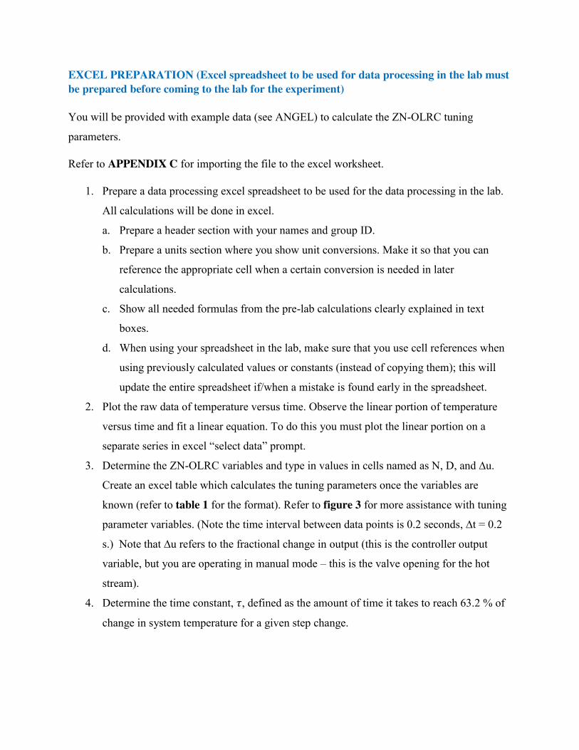
EXCEL PREPARATION (Excel spreadsheet to be used for data processing in the lab must be prepared before coming to the lab for the experiment) You will be provided with example data (see ANGEL) to calculate the ZN-OLRC tuning

parameters.

Refer to APPENDIX C for importing the file to the excel worksheet.

1. Prepare a data processing excel spreadsheet to be used for the data processing in the lab.

All calculations will be done in excel.

a. Prepare a header section with your names and group ID.

b. Prepare a units section where you show unit conversions. Make it so that you can

reference the appropriate cell when a certain conversion is needed in later

calculations.

c. Show all needed formulas from the pre-lab calculations clearly explained in text

boxes.

d. When using your spreadsheet in the lab, make sure that you use cell references when

using previously calculated values or constants (instead of copying them); this will

update the entire spreadsheet if/when a mistake is found early in the spreadsheet.

2. Plot the raw data of temperature versus time. Observe the linear portion of temperature

versus time and fit a linear equation. To do this you must plot the linear portion on a

separate series in excel “select data” prompt.

3. Determine the ZN-OLRC variables and type in values in cells named as N, D, and ∆u.

Create an excel table which calculates the tuning parameters once the variables are

known (refer to table 1 for the format). Refer to figure 3 for more assistance with tuning

parameter variables. (Note the time interval between data points is 0.2 seconds, ∆t = 0.2

s.) Note that ∆u refers to the fractional change in output (this is the controller output

variable, but you are operating in manual mode – this is the valve opening for the hot

stream).

4. Determine the time constant, 𝜏, defined as the amount of time it takes to reach 63.2 % of

change in system temperature for a given step change.

DATA PROCESSING Refer to APPENDIX C for importing the file to the excel worksheet.

1) Once you have collected all the necessary data, plot each run into appropriately named

excel sheet. Create a separate summary sheet where you copy and paste all the plots and

check with TA before leaving. (Note the time interval between data points is 0.2

seconds.)

KEY POINTS FOR REPORT See the separate file on ANGEL for the key report questions for level and temperature control.

APPENDIX A: Process Familiarization Before familiarizing with the process, turn on the cooling water so that the temperature can

stabilize (see appendix B step 1).

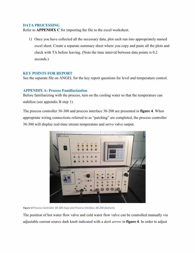
The process controller 38-300 and process interface 38-200 are presented in figure 4. When

appropriate wiring connections referred to as “patching” are completed, the process controller

38-300 will display real-time stream temperature and servo valve output.

Figure 4 Process Controller 38-300 (top) and Process Interface 38-200 (bottom).

The position of hot water flow valve and cold water flow valve can be controlled manually via

adjustable current source dark knob indicated with a dark arrow in figure 4. In order to adjust

either hot or cold water flow valve complete the figure 5 patching snapshot. There is no need to

switch Process Controller 38-300 on.

Figure 5 The wiring connections necessary for manual servo valve control. Note the dark adjustable knob indicated in arrow must be rotated between 0-20 mA in order to set the valve position. 0 mA corresponds to fully closed position and 20mA corresponds to fully open position.

Note the orange arrow pointing to the orange collar servo valve connector. The orange collar

wiring should be connected to either of the servo valve sockets in order to open or close the

hot/cold water valves. Orange collar wiring is exclusively used for servo valve control. Figure 6 indicates the connected state of orange collar wiring to the cold water flow valve. The

calibration between 0-10 can be seen on the cold water flow valve casing which corresponds to

the numerical indication of valve state. When the orange collar wiring is disconnected from the

cold water flow valve as shown in figure 6, the calibration will show zero but the valve state will

remain at the last used setting.

Figure 6 Snapshot rendition of the valve with and without electrical supply. Note the valve will remain at its position even when electrical connection is broken.

Both servo valves should be in fully open position. The user might check the valve positions in

both primary and secondary flow streams if unexpected circumstances arise, such as abnormal

stream temperatures.

The ABB COMMANDER 350 on Process Controller 38-300 as can be seen in figure 5 is a real

time stream temperature monitor and intermediary source to the chart recorder software on the

computer. The ABB COMMANDER 350 has already been appropriately set to the correct

settings, if in case any abnormalities in computer software chart recorder is intercepted the TA is

advised to refer to section 2.5.5 on the process manual provided by the vendor FEEDBACK (pdf

version can be found on ANGEL). It is highly recommended not to touch any buttons without

instructions.

The Thermistor Temperature Transmitter (TTT) and Digital Display Module (DDM) snapshot is

provided in figure 7. The TTT measures the temperature and relays the values electrically to the

DDM. TTT is already calibrated between temperatures 25 and 80 C. No calibration is necessary

upon each start-up and hence the TA is advised to go over the calibration if abnormal stream

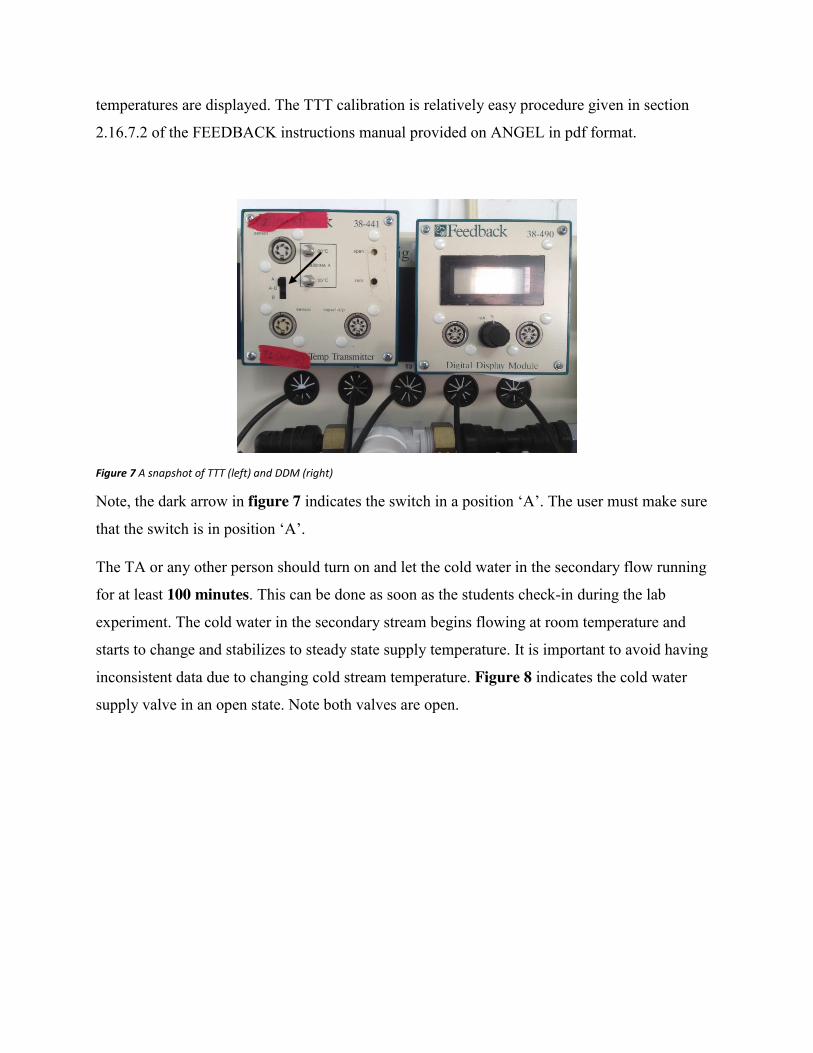
temperatures are displayed. The TTT calibration is relatively easy procedure given in section

2.16.7.2 of the FEEDBACK instructions manual provided on ANGEL in pdf format.

Figure 7 A snapshot of TTT (left) and DDM (right)

Note, the dark arrow in figure 7 indicates the switch in a position ‘A’. The user must make sure

that the switch is in position ‘A’.

The TA or any other person should turn on and let the cold water in the secondary flow running

for at least 100 minutes. This can be done as soon as the students check-in during the lab

experiment. The cold water in the secondary stream begins flowing at room temperature and

starts to change and stabilizes to steady state supply temperature. It is important to avoid having

inconsistent data due to changing cold stream temperature. Figure 8 indicates the cold water

supply valve in an open state. Note both valves are open.

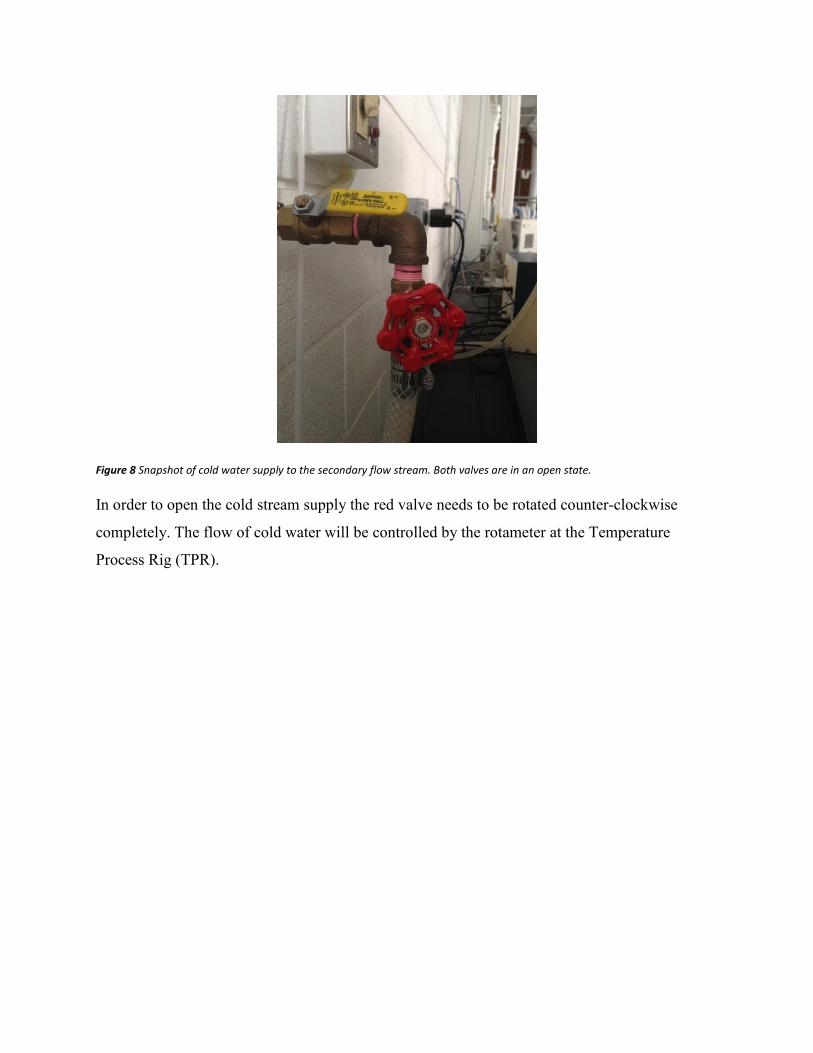
Figure 8 Snapshot of cold water supply to the secondary flow stream. Both valves are in an open state.

In order to open the cold stream supply the red valve needs to be rotated counter-clockwise

completely. The flow of cold water will be controlled by the rotameter at the Temperature

Process Rig (TPR).

APPENDIX B: Experimental Procedure 1) Turn on the cold water to the secondary flow by opening the valve on the rear of TPR.

Adjust the flow rate to 1-1.8 L/min by rotating the manual rotameter flow control valve.

Record the water flow rate. This should be kept constant during the experiment.

2) Turn on the computer next to the temperature process rig.

3) Complete the following patching diagram

Need to make sure the black switch (arrow indication) under the T5 connection is in “A”

position.

Refer to Section 2.20.3 Process Manual Instructions provided on ANGEL in ‘pdf’ format

if you are not sure about the above diagram. Alternatively, open Discovery II software on

the computer, select Procon process control trainers, then procon level and flow with

temperature for Modbus, then P PI PID Tempearature control, then Proactical 1:

proportional control, patching diagram – temperature procedure

The following pictures indicate the completed patching diagram;

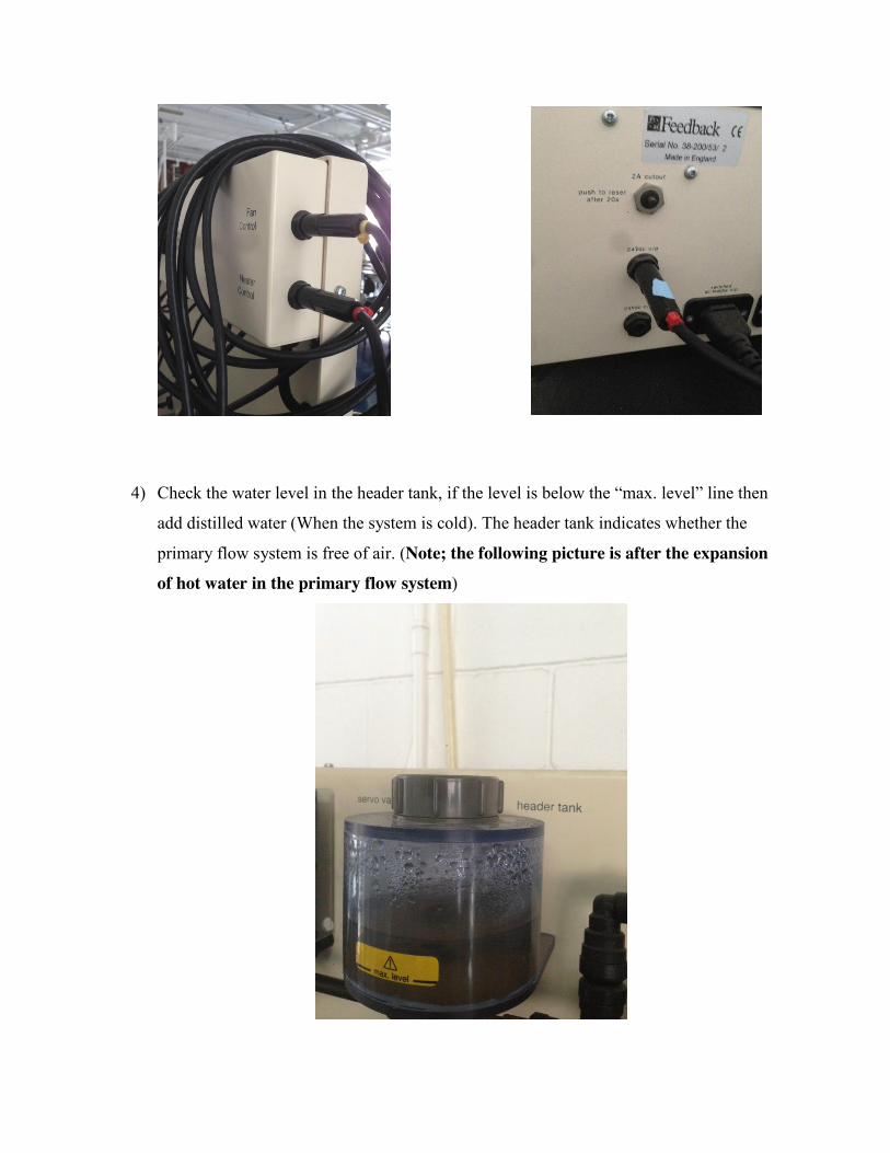
4) Check the water level in the header tank, if the level is below the “max. level” line then

add distilled water (When the system is cold). The header tank indicates whether the

primary flow system is free of air. (Note; the following picture is after the expansion of hot water in the primary flow system)

5) Turn on the process interface 38-200 by switching up the blue switch on the left corner of

the process interface 38-200. This will automatically cause the heater to start warming.

Allow ten minutes for the heater to warm up before proceeding to step 5. The heater is

controlled via thermostat between 65-70 ℃.

6) Turn on the power on process controller 38-300 by switching up the green switch on the

left corner of process controller 38-300.

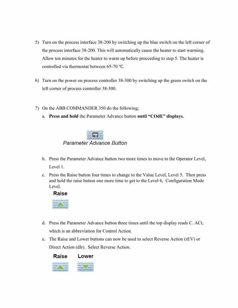
7) On the ABB COMMANDER 350 do the following;

a. Press and hold the Parameter Advance button until “COdE” displays.

b. Press the Parameter Advance button two more times to move to the Operator Level,

Level 1.

c. Press the Raise button four times to change to the Value Level, Level 5. Then press and hold the raise button one more time to get to the Level 6, Configuration Mode Level.

d. Press the Parameter Advance button three times until the top display reads C. ACt,

which is an abbreviation for Control Action.

e. The Raise and Lower buttons can now be used to select Reverse Action (rEV) or

Direct Action (dIr). Select Reverse Action.

f. Press the Parameter Advance button to return to the Level 6 display. (usually two

times press)

g. Press the Alarm Acknowledge button to return to the main operational display.

8) Switch on the TPR pump and cooling fan by switching both of the “switched ac supply

o/p” to the on position.

9) On the computer screen go to the “Discovery II IMS”. If prompted about explorer set-up

press “Ask me later”. On the page you can see another prompt “To help protect your

security…”, press on the prompt and on the drop-down menu select “Allow Blocked

Content…”, select “Yes”

10) Now you can see the content tree on the left of the

page. Expand the folders until you see the Chart

Recorder in the Process Control and Monitoring

Software folder.

11) Press on the “Chart Recorder”, wait for the prompt “Internet Explorer-Security Warning”

to appear, and then press “Run”. On the Chart Recorder you can see the “Set Point” and

“Process Variable” being displayed. The “Process Variable” corresponds to the

temperature “T5”.

12) On the ABB COMMANDER 350 make sure the yellow OP screen does display ‘M’ in

the lower left hand corner, which corresponds to manual process control. Press

Auto/Manual button until ‘M’ displays. Skip this step if you see ‘M’ on the OP screen.

13) You can change the “Set Point”, “Proportional”, “Integral”, and “Derivative” parameters

on the Chart Recorder. Make sure to press “enter” after every change. Carry out the open

loop Reaction Curve Tuning procedure as follows.

a. With ABB COMMANDER 350 in manual mode adjust the output (OP) to 5 using Up

and Down buttons. This is the percent opening of the primary (hot) water loop. Wait

until the system approaches the steady state as indicated by the Process Variable (PV)

screen on the Commander 350 unit. Record the steady state temperature ‘T5_OP5’ in

your notebook.

b. Adjust the set point (SP) to the value indicated on the steady state Process Variable

(PV) screen using Raise and Lower buttons.

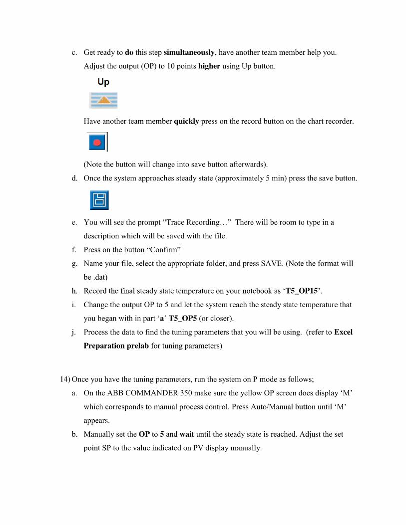
c. Get ready to do this step simultaneously, have another team member help you.

Adjust the output (OP) to 10 points higher using Up button.

Have another team member quickly press on the record button on the chart recorder.

(Note the button will change into save button afterwards).

d. Once the system approaches steady state (approximately 5 min) press the save button.

e. You will see the prompt “Trace Recording…” There will be room to type in a

description which will be saved with the file.

f. Press on the button “Confirm”

g. Name your file, select the appropriate folder, and press SAVE. (Note the format will

be .dat)

h. Record the final steady state temperature on your notebook as ‘T5_OP15’.

i. Change the output OP to 5 and let the system reach the steady state temperature that

you began with in part ‘a’ T5_OP5 (or closer).

j. Process the data to find the tuning parameters that you will be using. (refer to Excel Preparation prelab for tuning parameters)

14) Once you have the tuning parameters, run the system on P mode as follows;

a. On the ABB COMMANDER 350 make sure the yellow OP screen does display ‘M’

which corresponds to manual process control. Press Auto/Manual button until ‘M’

appears.

b. Manually set the OP to 5 and wait until the steady state is reached. Adjust the set

point SP to the value indicated on PV display manually.

c. Type in the P-only tuning parameter into the Chart Recorder. Increase the integral

parameter to a maximum and decrease derivative parameter to zero.

d. On the ABB COMMANDER 350 make sure the yellow OP screen does not display

‘M’ which corresponds to manual process control. Press Auto/Manual button until

‘M’ disappears.

e. Start recording the data by pressing on the record button.

f. Subject the system to ‘T5_OP15’ (Step 13. h) set point (SP) increase (max temp

achieved in open loop change) and wait until the steady state is reached. You can see

the % open of the valve on the Commander 350 display (OP), and you can hear it

open and close. Once the steady state has been reached press on save button.

This will take approximately 5-10 minutes.

g. You will see the prompt “Trace Recording…”

In the “description” space you can type in a description of the run. This will show up

as your sheet name in excel when you open the data as an excel file.

Press on the button “Confirm”

Name your file and Save your file in an appropriate folder.

h. Return to manual mode.

i. Change the output OP to 5 and let the system reach the steady state temperature that

you began with in part ‘a’ T5_OP5.

15) Follow the step 14) on P-only control again but use new parameter PB = 2 x PB_ZN-

OLRC value (twice the original value).

16) Follow the step 14) on P-only control again but use new parameter PB = 0.5 x PB_ZN-

OLRC value (half the original value).

17) Run the system on PI mode as follows;

a. On the ABB COMMANDER 350 make sure the yellow OP screen does display ‘M’

which corresponds to manual process control. Press Auto/Manual button until ‘M’

appears.

b. Manually set the OP to 5 and wait until the steady state is reached (T5_OP5 or

closer). Adjust the set point SP to the value indicated on PV display manually.

c. Type in the PI-only tuning parameters into the Chart Recorder. Decrease derivative

parameter to zero.

d. On the ABB COMMANDER 350 make sure the yellow OP screen does not display

‘M’ which corresponds to manual process control. Press Auto/Manual button until

‘M’ disappears.

e. Start recording the data by pressing on the record button.

f. Subject the system to ‘T5_OP15’ (step 13. h) set point (SP) increase and wait until

the steady state is reached. Once the steady state has been reached press on save

button. Approximately 5 minutes.

g. You will see the prompt “Trace Recording…”

In the “description” space you can type in a description of the run. This will show up

as your sheet name in excel when you open the data as an excel file.

Press on the button “Confirm”

Name your file and Save your file in an appropriate folder.

h. Return to manual mode.

i. Change the output OP to 5 and let the system reach the steady state temperature that

you began with in part ‘a’ T5_OP5.

18) Follow the step 17) on PI-only control again but with a new integral time Ti = 2x Ti_ZN-

OLRC (twice the original integral time).

19) Follow the step 17) on PI-only control again but with a new integral time Ti = 0.5x

Ti_ZN-OLRC (half the original value).

20) Run the system on PID mode as follows;

a. On the ABB COMMANDER 350 make sure the yellow OP screen does display ‘M’

which corresponds to manual process control. Press Auto/Manual button until ‘M’

appears.

b. Manually set the OP to 5 and wait until the steady state is reached (T5_OP5 or

closer). Adjust the set point SP to the value indicated on PV display manually.

c. Type in the PID-only tuning parameters into the Chart Recorder.

d. On the ABB COMMANDER 350 make sure the yellow OP screen does not display

‘M’ which corresponds to manual process control. Press Auto/Manual button until

‘M’ disappears.

e. Start recording the data by pressing on the record button.

f. Subject the system to ‘T5_OP15’ (step 13 h.) set point (SP) increase and wait until

the steady state is reached. Once the steady state has been reached press on save

button.

g. You will see the prompt “Trace Recording…”

In the “description” space you can type in a description of the run. This will show up

as your sheet name in excel when you open the data as an excel file.

Press on the button “Confirm”

Name your file and Save your file in an appropriate folder.

h. Return to manual mode.

i. Change the output OP to 5 and let the system reach the steady state temperature that

you began with in part ‘a’ T5_OP5.

21) Repeat step 20) on PID-only control but use the simplified IMC PID parameters.

SHUTDOWN 22) On the ABB COMMANDER 350 make sure the yellow OP screen does display ‘M’

which corresponds to manual process control. Press Auto/Manual button until ‘M’

appears.

23) Manually set the OP to 5.

24) Switch the Process Controller 38-300 off by turning the green power switch down.

Switch the Process Interface 38-200 off by turning the blue power switch down.

Disconnect the patching wires and store in the drawer beneath the table.

25) Close the cold water supply valves indicated in figure 8.

26) Process all the data and check with TA before leaving.

APPENDIX C : Opening Data in Excel 1. Open Excel.

2. Go to File>>Open.

3. Switch from “All Excel Files” to “All Files” and open your .dat files.

4. A Text Import Wizard will now appear.

5. Choose Delimited>>Next.

6. In Delimiters, check Tab and Comma>>Next.

7. Click Finish. Click OK

8. You will only need 2 columns of data; 1st column Stream Temperature, 2nd column

Process Output. 9. Copy your data into your spreadsheet workbook to fully analyze.