Journal of Structural Engineering Vol. 67A (March 2021) JSCE

Temperature variation on different colored steel plates

Caused by solar radiation

Ruobing Sun†, Yasuo Suzuki*, Tomonori Tomiyama**, Yasuo Kitane***,

Kuo-chun Chang****, Kunitomo Sugiura*****

†Ms. of Global Environmental Studies., Dept. of Civil and Earth Resources Eng., Kyoto University, Nishikyo-ku, Kyoto 615-8540

*Dr. of Eng., Assoc. Professor, Dept. of Civil Design and Eng., Toyama University, Toyama 930-8555

**Dr. of Eng., iMaRRC, Public Works Research Institute, 1-6 Minamihara, Tsukuba 305-8516

***Ph.D., Assoc. Professor, Dept. of Civil and Earth Resources Eng., Kyoto University, Nishikyo-ku, Kyoto 615-8540

****Ph.D., Professor, Dept. of Civil Eng., National Taiwan University, Taipei 106, Taiwan

*****Ph.D., Professor, Dept. of Civil and Earth Resources Eng., Kyoto University, Nishikyo-ku, Kyoto 615-8540

Abstract: This paper presents the temperature variation of steel structures with different colors

subjected to solar radiation by means of experiments. Steel plate specimens of standard size with

different colors were exposed to sunlight to measure temperature changes over the course of a day

in various places. Then, a one-dimensional heat conduction model is established to simulate the

output surface temperature of steel plate specimens by using the environmental parameters

obtained from experiment, and the numerical results are compared with the experimental results

to prove its feasibility. On the basis of this model, the influence of different factors on the

temperature change of steel structures is studied.

Keywords: steel, solar radiation, temperature distribution, paint color

1. INTRODUCTION

In recent years, steels have been widely used in bridges owing

to their excellent material properties and being reliable by industrial

manufacturing and transportation. In the long-term operation, the

steel bridge is subjected to many variable actions. The temperature

change caused by solar radiation is a kind of short-term change.

The sun rises from the east, and goes up to the south and finally

down in the west, so that solar radiation to steel structures’ surface

always change. Thermal stress or deformation caused by a

temperature change due to solar radiation on structure is non-

uniform and may cause component damage or even destruction,

which buries an unpredictable risk for bridge safety. Accidents of

structures caused by temperature effect of solar radiation have

occurred all over the world. The DuSable Bridge in Chicago

stopped working due to unbearable heat under sunlight in 20181).

The surface temperature of the bridge had risen above 60℃ in such

week, which caused the steel bridge expanded sideways and steel

components started rubbing each other and caused friction in

between. The bridge lost the capacity of opening for boats and had

to stop serving for half an hour for firefighters hosing it down with

cold water. What else, the three-span, continuous Fourth Danube

Bridge collapsed largely because of temperature effects2). During

the construction, when both cantilever sides of the center span were

joined in daytime, the workers had to shorten the span because of

the expansion caused by high temperature, while at night the bridge

shrunk. The compression in the lower flange along with the use of

flat bar stiffeners, caused the bridge to buckle near the right-hand

dead load moment contraflexure point in middle span, and then at

the mid of side span and finally got into a third buckle3).

Many efforts have been made into studying the characteristics

of temperature variation of bridges under solar radiation. Taniguchi

† Corresponding author

E-mail: sun.ruobing.46z@st.kyoto-u.ac.jp

-452-

conducted an experimental study on the surface temperature

change of steel in different coating colors caused by direct

sunlight4), and measured the temperature difference of the test steel

in different coating colors in direct sunlight and in direct sunlight

without infrared rays. Chen has measured the solar radiation

absorption coefficient of coatings commonly used for steel

structure based on spectrometric method5). Hashimoto measured

the daily temperature changes of composite Trussed Rohze Bridge

with SRC Structure in different components under direct sunlight,

and obtained the stress and deformation caused by temperature

load through FE model simulation6). Okumura measured the

temperature of a steel concrete composite truss railway bridge by

installing thermal couples both inside and outside the truss7). Xia

has conducted the monitoring of Humber Bridge to figure out the

temperature distribution combining with stimulation8).

In this paper, the temperature of a group of steel specimens

with different coating colors under direct sunlight is measured

during daytime with thermocouples. Through collecting the data

of the daily temperature change of the same group of steel plate

specimens under sunlight in different environments, such as Kyoto,

Kobe, Nago, and Taipei, the characteristics of the temperature

change of the steel plate specimens under sunlight are obtained.

Moreover, different parameters as ambient temperature, solar

radiation intensity, wind speed, setting angle and color are also

discussed to study their influence on the surface temperature

distribution of the steel specimens.

Secondly, based on the theory of heat transfer, a one-

dimensional heat conduction model is established to simulate the

output surface temperature of steel plate specimens by using the

environmental parameters recorded in the experiment, and the

numerical results are compared with the experimental results to

prove its feasibility. On the basis of this model, the influence of

ambient temperature, solar radiation intensity and wind speed on

the temperature change of steel specimens is studied by the control

variable method, and the recommended values of solar radiation

absorption coefficient of steel specimens with different colors are

assessed.

2. EXPERIMENT PROGRAMS

2.1 Experiment specimens

Experimental specimens are 8 pieces of steel plates

(5mm×70mm×150mm), of which 7 are painted anticorrosive

coating by professional factory to ensure coating surface uniform

and smooth, while one only does the shot blasting process. In this

experiment, common painting colors in actual bridges were

considered. Combining the factors of original colors of materials

and the three primary colors of red, green and blue, eight typical

colors were selected as research samples. The code of each color is

accurately classified as shown in Table 1, using the JPMA

Standard Paint Color Code (2019, K version) 9). The details of the

coating of specimens are described in this table:

The actual setting of specimens at the experiment site is shown

in Fig.1. The specimens are fixed on the styrene foam plate with

small plastic clippers and arranged in staggered order to prevent the

influence from each other. The back side of the foam plates is fixed

with iron frame and restraint belt, to make sure that the specimens

are isolated from the heat of the iron frame.

2.2 Experiment conduction

The experiments are conducted in 4 places (Fig.2):

⚫ Taipei (25°04'04.6"N,121°39'09.0"E);

⚫ Nago(26°38'44.4"N,128°04'50.2"E);

⚫ Kobe(34°42'35.3"N 135°17'35.5"E) and

⚫ Kyoto(34°58'56.7"N,135°40'37.2"E).

Fig.1 Steel specimens with different colors

under direct sunlight

Fig.2 Experimental locations

Table 1 Painting specification of steel specimens for exposure test

No. Color Code Coating Remark

1 White KN-95 C-5

Surface and

round edge are

painted.

2 Grey KN-65 C-5

3 Blue K69-50T C-5

4 Green K39-40P C-5

5 Red K07-40X C-5

6 Brown K09-40L C-5

7 Black KN-30 C-5

8 - - No

coating

Shot blasting on

both sides

-453-

The four cities are distributed in different latitudes and

longitudes and have different climates. Kobe has a similar

longitude to Kyoto, and Taipei has a similar longitude to Nago and

is closer to the equator, with higher summer temperatures. Kobe

and Nago are near the coast, where wind in the winter is stronger.

Select these four cities to collect a wider variety of data.

The experimental measurement includes the temperature of

the specimen, ambient temperature, wind speed and solar radiation

intensity. For temperature measurement, K - type thermocouple

sensors are used to measure the real-time temperature of specimens.

One end of the compensating wire is attached to the surface of

specimens with tape, while the other end is connected to

thermocouples. For temperature recording, in Taipei, handheld

data logger (TC-32K, accuracy of 0.1 degree) is used for

measuring the temperature of specimens. The measurement time

is 10AM to 4PM, according to actual weather condition. The

measurement interval is one hour. In Kyoto, Kobe and Nago, the

data logger with 12 channels (SATO BTM-4208SD) is used for

recording, accuracy of 0.1℃. Ambient temperature and wind

speed are measured using a portable weather meter (Kestrel 5500).

The intensity of solar radiation is measured by Illumination-solar-

UV Meter (Tenmars, TM-208_Solar, UVA & Light Meter 3 in 1).

All the data is automatically recorded, and the effective time of

recording each day is from 7AM to 6PM. The recording interval is

10 minutes.

2.3 Result

When the component is under the condition of clear and

cloudless, high radiation intensity, high ambient temperature and

low wind speed, its temperature rise under sunshine is higher.

Based on the comprehensive comparison of all the test data, this

paper selects several specific days with relatively obvious

temperature change in each region as typical days, and takes it as

an example to study the surface temperature of the specimens.

The typical results are shown in the figures below, Figs.3-8.

The results shown in the figure are average value per hour.

Fig.3 shows the result in Taipei. As it can be seen from the

figure, in different time periods, the temperature variation trend of

each specimen is generally the same, which is a parabola. The

direct sunlight has an obvious influence on the temperature on the

steel specimens. The darker the color is, the more evident the result

would be. The maximum temperature is up to 54.9℃, which

shows up on black specimen, while the environment temperature

was 27.7℃. At the same time, the maximum of temperature

difference is 18.3℃.

Fig.4-6 indicates the result in Nago, Okinawa. The ambient

temperature of Nago is about 10℃ higher than that of Taipei as a

whole, and the solar radiation intensity is also higher, which makes

the maximum surface temperature of the whole set of steel

specimens about 15℃ higher than that measured in Taipei. The

maximum temperature of the specimen still appears on black

specimen, and the average temperature reached to 64℃.

In all the data of Okinawa, there is a rapid temperature rise of

the specimen at 9AM. On the one hand, the specimen was no

longer sheltered and completely exposed to the sunlight. On the

other hand, the residual dew or condensation from the rain in the

morning on the specimen affected the temperature of the specimen

before 9AM.

Fig.3 Temperature change of steel specimens

on November 30th, Taipei TAIWAN

Fig.4 Temperature change of steel specimens

on July 26th, Nago JAPAN

Fig.5 Temperature change of steel specimens

on July 28th, Nago JAPAN

-454-

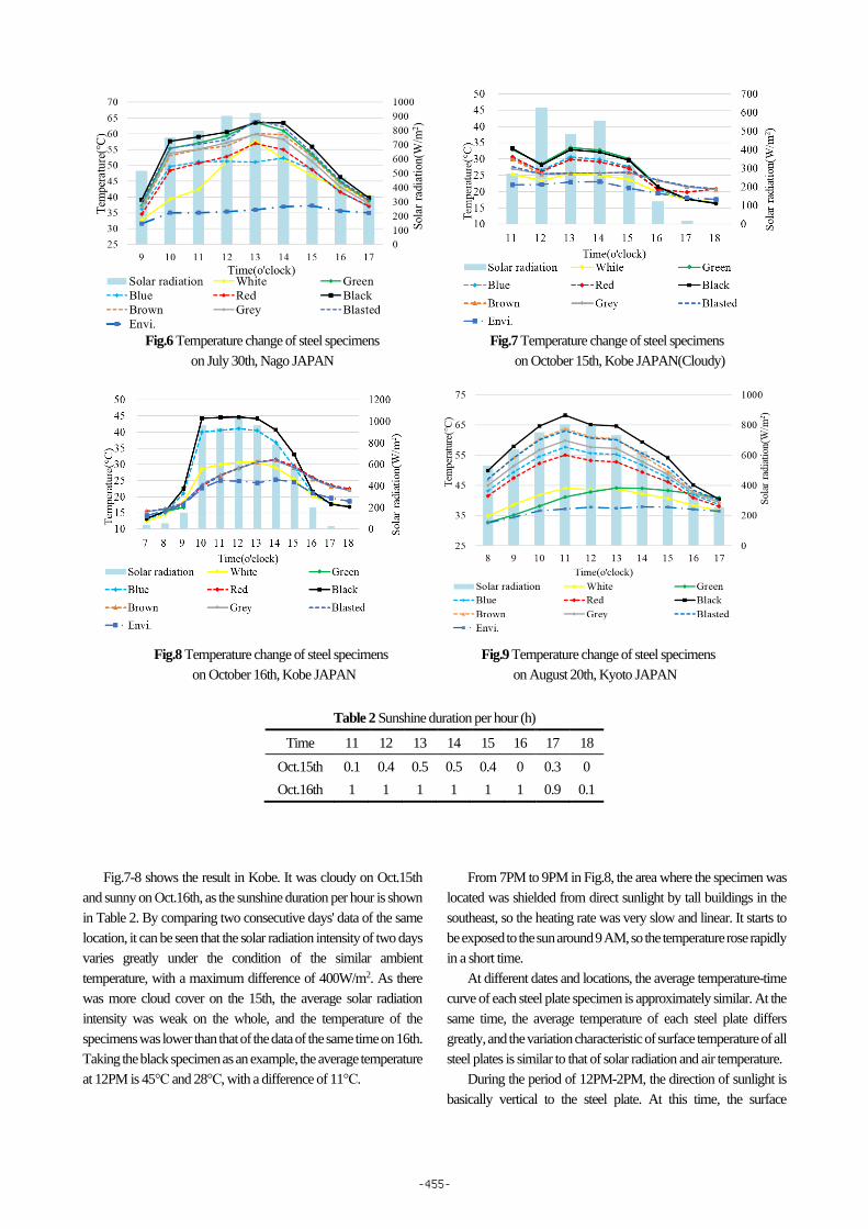
Fig.6 Temperature change of steel specimens Fig.7 Temperature change of steel specimens

on July 30th, Nago JAPAN on October 15th, Kobe JAPAN(Cloudy)

Fig.8 Temperature change of steel specimens Fig.9 Temperature change of steel specimens

on October 16th, Kobe JAPAN on August 20th, Kyoto JAPAN

Table 2 Sunshine duration per hour (h)

Time 11 12 13 14 15 16 17 18

Oct.15th 0.1 0.4 0.5 0.5 0.4 0 0.3 0

Oct.16th 1 1 1 1 1 1 0.9 0.1

Fig.7-8 shows the result in Kobe. It was cloudy on Oct.15th

and sunny on Oct.16th, as the sunshine duration per hour is shown

in Table 2. By comparing two consecutive days' data of the same

location, it can be seen that the solar radiation intensity of two days

varies greatly under the condition of the similar ambient

temperature, with a maximum difference of 400W/m2. As there

was more cloud cover on the 15th, the average solar radiation

intensity was weak on the whole, and the temperature of the

specimens was lower than that of the data of the same time on 16th.

Taking the black specimen as an example, the average temperature

at 12PM is 45℃ and 28℃, with a difference of 11℃.

From 7PM to 9PM in Fig.8, the area where the specimen was

located was shielded from direct sunlight by tall buildings in the

southeast, so the heating rate was very slow and linear. It starts to

be exposed to the sun around 9 AM, so the temperature rose rapidly

in a short time.

At different dates and locations, the average temperature-time

curve of each steel plate specimen is approximately similar. At the

same time, the average temperature of each steel plate differs

greatly, and the variation characteristic of surface temperature of all

steel plates is similar to that of solar radiation and air temperature.

During the period of 12PM-2PM, the direction of sunlight is

basically vertical to the steel plate. At this time, the surface

-455-

temperature reaches the maximum value and the temperature

difference between the steel plates reaches the maximum value as

well.

Among all the experimental data, the highest value of surface

temperature appeared on the black specimen, which reached

68.8℃ on August 20th, 2020(Fig.9). At the same time, the surface

temperature of the white specimen is only 44℃, that is, the

maximum temperature difference between the specimens is

24.2℃. The ambient temperature is 37.1℃, that is, the temperature

difference between the specimen and the environment is 31.1℃.

3. NUMERICAL SIMULATION METHOD

3.1 Theoretical basis of one-dimensional heat conduction

model

The temperature field T of a cross section at time t may be

expressed by Poisson equation models for the three-dimensional

(3D) transient heat flow process, representing the heat traveling

through a homogenous solid via conduction10):

𝑘 (𝜕2𝑇

𝜕𝑥2 +𝜕2𝑇

𝜕𝑦2 +𝜕2𝑇

𝜕𝑧2) = 𝜌𝑐∂𝑇

𝜕𝑡 (1)

where T is the temperature represented by the Cartesian

coordinates (x, y, z), k is the thermal conductivity; ρ is the density

of the component, c is the specific heat capacity of the component

material, and t is time.

In the natural environment, the bridge structure is exposed to

direct solar radiation, scattered radiation and other kinds of

radiation:

𝑘𝜕𝑇

𝜕𝑛+ 𝑞 = 0 (2)

where q (unit W/m2) is the heat flux on the component surface,

including convective heat transfer heat flux qc, radiant heat flux qr

on the component surface, and solar radiation heat flux qj, which is

𝑞 = 𝑞𝑐 + 𝑞𝑟 + 𝑞𝑗 (3)

The heat flux qc of component surface loss due to heat

convection is

𝑞𝑐 = ℎ(𝑇𝑠𝑢𝑟 − 𝑇𝑎𝑖𝑟) (4)

ℎ = 5.8 + 4.0𝑣 (5)

where h (W/(m2•K)) is the convection heat transfer coefficient, v

is wind speed and Tsur and Tair are the component surface

temperature and atmospheric temperature, respectively. Equation

5 is Jurges formula11), which is a simple formula which only takes

convective heat transfer rate as wind speed function and is proved

reasonable by previous observation data. Previous studies have

shown that h is mainly related to wind speed and has nothing to do

with the material itself.

The heat flux radiated from the surface of the member to the

sky is:

𝑞𝑟 = 𝜀𝜎(𝑇𝑠𝑢𝑟)4 (6)

where ε is the radiation coefficient of the member, σ is Stefan-

Boltzmann constant which is the total energy radiated from a black

body per unit surface area, per unit time.

The heat flux of solar radiation received by the component:

𝑞𝑗 = −𝛼𝐽0 (7)

where α is solar radiation absorption coefficient of the surface

material (between 0 and 1), and J0 is the intensity of solar radiation.

Then, the whole heat flux on the surface of the steel member

can be described as:

𝑞 = 𝑞𝑐 + 𝑞𝑟 + 𝑞𝑗 = (5.8 + 4.0𝑣)(𝑇𝑠𝑢𝑟 − 𝑇𝑎𝑖𝑟) +

𝜀𝜎(𝑇𝑠𝑢𝑟)4 − 𝛼𝐽0 (8)

where Tair, J0 and v are known values that change with time.

The experimental value is compared with the simulated value.

Through the comparison of the measured data between July

and November, the environmental data of July 30th, September

8th, October 16th and November 10th are selected to simulate the

daily temperature change of steel specimens. The measured

environmental parameters which means solar radiation intensity,

ambient temperature and wind speed, are input according to the

measured data, and the other coefficients involved are set as close

as possible to the actual conditions of the environment and the

specimen.

In this paper, the ability of the sample to absorb solar radiation

is reflected by the solar radiation absorption coefficient, and the

color affects the size of the solar radiation absorption coefficient.

Therefore, only the solar radiation absorption coefficient is

discussed, and the steel sheet defaults to the same radiative

coefficient. Other coefficients are set as follows, which is decided

by the material property of steel specimens:

𝜀 = 0.85

𝜎 = 5.67 × 10−8 𝑊/(𝑚2 ∙ 𝐾4)

𝑘 = 56 𝑊/(𝑚 ∙ 𝐾)

On this basis, the one-dimensional heat conduction model is

established. Based on the established model, the approximate

numerical solution is obtained by using the difference method, and

the numerical solution is transformed into the approximate solution,

that is, the equation is dispersed to each node and then the

numerical approximate solution is calculated.

The forward difference scheme of one-dimensional heat

conduction is established as12):

𝜕𝑇

𝜕𝑡≈

(𝑇𝑠𝑢𝑟)𝑛+1−(𝑇𝑠𝑢𝑟)𝑛

∆𝑡 (9)

The initial surface temperature depends on the ambient

temperature at the initial time. In this paper, it is considered that

when the solar radiation intensity is very small, the surface

temperature of the specimen is assumed to be equal to the ambient

temperature.

3.2 Simulation result

The equations are solved on the basis of Matlab13), and the

results are shown in Figs.10-13, using black color as an example,

as it has the most obvious temperature change during the day:

The figure shows the temperature comparison between the

-456-

Fig.10 Data comparison (July 30th)

Fig.11 Data comparison (September 8th)

Fig.12 Data comparison (October 16th)

Fig.13 Data comparison (November 10th)

experimental results and the simulation results of the steel

specimens under different environmental conditions in different

regions. As can be seen from Fig.10-13, the numerical simulation

results of the steel specimens are basically in agreement with the

measured results.

However, there are some differences between curves of the

measured data and the simulated data, such as the lag between the

2 curves. The reasons may be: (1) the time delay of heat transfer

between environment and steel plate; (2) the rapid change of

environment parameters during the interval time; (3) the cloudy

weather condition; and (4) the ignoring the heat transfer with

ground.

4. PARAMETIC STUDIES

Use the control variate method to consider the influence of

different parameters. In the discussion of control variables, each

parameter in Equation (8) is replaced with different values by

multiplying the original experimental data to a proportionality

coefficient, and the output results of the program are obtained. On

this basis, the influence of each parameter could be discussed.

4.1 Solar radiation

Limited by the solar radiation constant, the value of solar

radiation to a region does not rise indefinitely. The solar constant

refers to the solar radiation received per second per unit area

perpendicular to the sun's rays at the mean distance between the

sun and earth (D=1.496x108 km). It is a relatively stable constant,

generally taken as 1367W/m2, floating at ±1%.

Use the control variate method to consider the influence of

solar radiation. By multiplying to a proportionality coefficient, the

value of solar radiation is assumed as 80%, 60%, 40%, 20% and 0

of the measured data (as which is shown in the figure as 0.8, 0.6,

0.4, 0.2, 0), using the data of September 8th, while remaining the

other variates as the original measured value. The result is shown

as Fig.14. The original simulation result of 100% solar radiation

intensity was shown in Fig.11.

According to the theoretical formula and the measured data,

the solar radiation intensity is positively correlated with the surface

temperature of steel members. The higher the intensity of solar

radiation, the higher the surface temperature distribution of steel

members exposed to direct sunlight. Taking the simulation data of

September 8th as an example, the temperature of steel sheet

reached the highest around 12PM, and the difference of the

maximum temperature of steel specimens under different solar

radiation could reach 10 degrees. From the figure, it can be seen

that solar radiation intensity influences the fluctuation degree of the

temperature curve, that is, the difference between the highest

temperature and the lowest temperature and the maximum value

of surface temperature, while it has almost no relation with the

minimum value.

4.2 Ambient temperature

Similar to the above method, the influence of ambient

temperature is considered by reducing it with the same value

(6.6℃, 13.3℃, 20℃, 27.7℃, 33℃ as which is shown in the

figure), using the data of September 8th. The result is shown as

Fig.15.

0

10

20

30

40

50

60

70

9 10 11 12 13 14 15 16 17

Tem

per

atu

re(℃

)

Time(o'clock)

Experiment Simulation

0

10

20

30

40

50

60

7 8 9 10 11 12 13 14 15 16 17 18

Tem

per

atu

re(℃

)

Time(o'clock)

Experiment Simulation

0

10

20

30

40

50

60

7 8 9 10 11 12 13 14 15 16 17

Tem

per

atu

re(℃

)

Time(o'clock)

Experiment Simulation

-457-

Fig.14 Influence of solar radiation

Fig.15 Influence of ambient temperature

Fig.16 Influence of wind speed

It can be seen from the theoretical formula and the measured

value that the ambient temperature is also positively correlated with

the surface temperature of the steel specimens. The higher the

ambient temperature is, the higher the daily temperature

distribution of the steel surface temperature can be. Each time the

environmental temperature value is lowered by about 7℃, the

overall temperature distribution of the steel specimens drops by

7 ℃ evenly. However, different from solar radiation, it can be seen

from the figure that the daily variation curves of steel surface

temperature are parallel to each other when the ambient

temperature is different. Therefore, the ambient temperature

determines the distribution range of the maximum and minimum

intra-day surface temperature of the steel specimens, but does not

affect the difference between the minimum and maximum.

4.3 Wind speed

By multiplying to a proportionality coefficient, the value of

wind speed is assumed as 120%, 140%, 180%, 50% and 0 of the

measured data (as which is shown in the figure as

0%,50%,120%,140%,180%), using the data of September 8th,

while remaining the other variates as the original measured value.

The result is shown as Fig.16.

Wind speed is an important factor determining the value of

convective heat transfer coefficient. The larger the wind speed is,

the more severe the convective heat exchange between the

environment and the surface of the component will be, and the

closer the surface temperature of the component is to the ambient

temperature. As shown in the figure, the influence of wind speed

on the surface temperature of steel specimens is not obvious. The

maximum temperature difference between the state without wind

speed and the state with original wind speed is about 5℃, and the

minimum value has no significant change. It can be seen that wind

speed has an influence on the overall temperature distribution of

the surface temperature of the steel specimens, but the influence of

wind speed is relatively limited under the conditions of non-

extreme weather in normal areas.

4.4 Angle

During the day, the sun rises in the east and sets in the west.

The relative position of the sun and the structure leads to different

solar radiation intensity on the surface of the structure facing

different angles and it changes at any time. To take the effect of the

angle on the surface temperature of specimen into consideration,

the temperature distributions of the specimens were recorded under

the four conditions of horizontal placement, 45 degrees of included

angle between the specimen and the ground facing east, 45 degrees

of included angle between the specimen and the ground facing

west, and being perpendicular to the sun at all times. The results are

shown in Figs.17-20.

Because the specimens are facing the east direction (Fig.18),

they are exposed to direct sunlight before noon comes. The

temperature peak arrives earlier that of specimens which are

horizontally installed, which is 52.7ºC on the black specimen

around 11AM. The temperature distribution distinguishes very

obviously before and after 12PM. After 12PM, the temperature

drops with an apparent tendency and the difference between

components are much smaller, as the angle of sunlight gradually

turns to be parallel to the specimens.

On contrary to the specimens facing east 45°, the specimens

facing west 45° receive more sufficient sunlight after 12PM

(Fig.19). For example, at 4PM in the afternoon, the black specimen

is 56.5 ºC, while in Fig.18, it is only 35 ºC. The environmental

temperature are 34.8 ºC and 33.8 ºC, of which the difference can

be ignored. However, at the same time, the solar radiation is 940

W/m2 and 79.2 W/m2, which is about 12 times to each other.

-458-

Fig.17 The specimen and solar meter installed

on the theodolite

Fig.18 Temperature change of steel specimens

(east 45degrees)

Fig.19 Temperature change of steel specimens

(west 45degrees)

Fig.20 Temperature change of black specimen

tracking the sun

A theodolite is used to follow the track of the sun (Fig.17). By

fixing the specimen and solar meter on the theodolite, the specimen

can always face vertically to the sunlight, so as the solar meter to

record the direct solar irradiance during daytime.

In Fig.20, since the specimen has always been facing the sun,

the temperature changes are relatively mild comparing to that of

specimen installed in one direction, ranging from 40℃ to 50℃

from 11AM to 4:30PM. The weather was a bit cloudy, so there

were sometimes breaks in the solar radiation. After 5PM, the sun

was covered by clouds, and the sunlight support was insufficient,

so the temperature fell rapidly.

It could be seen from figures that the angle of the specimens

has clear influence on the solar radiation received by the surface of

specimen, which could be combined with the influence of solar

radiation.

4.5 Colors

The color of steel coating is an important factor influencing the

absorption coefficient of solar radiation. When the material and

surface smoothness of the object have been determined, the coating

color will play a decisive role. Different coating colors correspond

to different radiation absorption coefficients. In general, the darker

the color is, the greater the solar radiation absorption coefficient

should be, and the more obvious the temperature rise and fall of the

steel component surface can be under direct sunlight.

In order to accurately simulate the temperature change of steel

specimens with different colors under solar radiation, it is very

important to determine the solar radiation absorption coefficient of

each color. Considering the hysteresis of temperature change

caused by environmental factors, the simulated temperature curve

is optimized by adjusting the value of solar radiation absorption

coefficient for each color.

In this section, the group of data on November 10th is used as

an example. Taking the simulated temperature result as the Y-axis

and the measured result as the X-axis, the scatter graph can be

established as shown in Fig.21. When R2, the coefficient of

determination of the trend line of the scatter graph is greater than

0.9, it is considered that the value of α meets the requirements. For

example, Fig.21 indicates the fitting degree of the red specimen

when setting the absorption coefficient as 0.1.

According to this standard, the solar radiation absorption

coefficient of each color is obtained, as shown in Table 3. The

output results for different colors are also shown in Figs.22-29.

By comparing the simulation results with the measured results,

it was found that the specimens with different colors could be

divided into two groups: black, gray, white and blue specimens

show a significant change range with solar radiation, while brown,

red, green and blasted specimens show a small change range of

temperature affected by the environment.

-459-

Fig.21 Comparison between experimental result and simulation

result

Table 3 Absorption coefficient of each color

White Grey Blue Green

0.13 0.27 0.24 0.1

Red Brown Black Blasted

0.1 0.1 0.3 0.1

Fig.22 Data comparison on white specimen

Fig.23 Data comparison on green specimen

Fig.24 Data comparison on blue specimen

Fig.25 Data comparison on red specimen

Fig.26 Data comparison on brown specimen

Fig.27 Data comparison on black specimen

Fig.28 Data comparison on grey specimen

Fig.29 Data comparison on blasted specimen

0

5

10

15

20

25

30

0 10 20 30

Exp

erim

enta

l re

sult

(℃)

Simulation result(℃)

White

Green

Black

Brown

Grey

Blasted Blue

Red

-460-

It is worth noting that the absorption coefficient of white plate

is higher than that of some other colors. Considering the reason

might be the following: The experimental data picked to use is

relatively data of latter part when the surface coatings of each

specimen have had some changes. As the former result shows, the

sensitivity of the brown and bare specimens to the intensity of solar

radiation is quite similar to that of the black one, but in

experimental data after August, it decreased significantly. The

reason may be that the anticorrosion coating on the surface of the

specimen was worn by the rain, and the surface of the specimen

was rusted, which changed the relevant characteristic parameters.

In addition, the atmospheric temperature at the later stage of the

experiment was relatively low and the overall temperature

amplitude was not high, so the difference between absorption

coefficients was not large.

In general, although the numerical simulation results have

obvious lag, the numerical simulation results have similar trend

with the measured results, indicating that the numerical simulation

method is applicable.

4.6 Size

To compare the influence on the size of specimens, another

experiment was conducted to measure the temperature of a group

of steel specimens (Group B) with different sizes but same color,

and recorded its change over the course of a day. The size of the

specimens are shown in Table 4 below. This experiment is

conducted from 8:30AM to 17:30PM from July 26th to July 28th,

Nago.

The measuring points are shown in Fig.30, which are 7 sensors

in total. This experiment focuses on three specimens to study the

temperature distribution of a single specimen at different positions

under different sizes. In Fig.30, SPECIMEN 1 is a long specimen.

The sensors are located at the leftmost edge (Sensor 1), at 1/2

(Sensor 2), at 3/4 (Sensor 3) and at the rightmost end (Sensor 4)

from left to right. In addition, the leftmost end of SPECIMEN 1 is

covered by cardboard which does not touch the specimen, so as to

study the heat transfer of the specimen without direct sunlight.

SPECIMEN 2 is square, Sensor 5 is placed horizontally in the

middle of SPECIMEN 2, and Sensor 6 is placed horizontally in the

bottom edge of SPECIMEN 2. Sensor 7 is located in the middle of

SPECIMEN 3 and parallel to the long side. All sensors are placed

on the back of the specimen and fixed tightly with tape.

The result is shown in Figs.31-32. As can be seen from the two

figures, in the overall temperature distribution, the middle point of

the long specimen (SPECIMEN 1) has the highest temperature

value. The temperature distribution of SPECIMEN 1 decreases

from the middle to the edge, which means highest temperature

appears at Sensor 2 and the lowest at Sensor 4. The temperature

distribution of SPECIMEN 2 is also significantly higher in the

middle than in the edge. The temperature of SPECIMEN 3 as a

whole is close to the middle part (Sensor 6) of SPECIMEN 2.

Fig.30 Location of measuring points on Group B(unit:mm)

-461-

Table 4 Sizes of Group B specimens

No. Color(code) Size(mm) Measuring point

1

Dark brown

(K05-30B)

150 * 900 4 measuring points in wider direction

2 300 * 300 2 measuring points in diagonal direction

3 150 * 70 1 measuring point

Fig.31 Temperature change of Group B specimens

on July 27th

Fig.32 Temperature change of Group B specimens

on July 28th

The highest temperature shows up at Sensor 2, which is 68.8℃.

At the same time, the temperature at Sensor 1 is 57.8℃ and the

temperature at Sensor 4 is 63.8℃. The temperature difference on

the SPECIMEN 1 under direct sunlight is 5℃. For the same

specimen, the temperature difference between direct sunlight and

shadow is 11℃. When the size of the components is larger and the

structure is more complex, the heat conduction between the

components will be more complicated, which will lead to more

complex time-varying temperature effect.

On the other hand, it is worth noticed that the temperature

difference on SPECIMEN 2 is about 5℃ as well. The reason may

be that the volume of the specimens differs from each other, the

heat capacity is different. What’s more, due to the wider edge and

more cantilever parts, SPECIMEN 2 was exposed to more air flow

and dissipated heat faster than SPECIMEN 1.

5. CONCLUSIONS

From this study the following conclusions are obtained:

1） By studying the surface temperature changes of different steel

sheet samples under solar radiation, it is found that under the

condition of the same size and different colors, the

temperature peak of the dark-colored samples is higher, with

a maximum of 68.8 degrees of black specimen; Under the

condition of the same color and different size, the temperature

distribution on the same specimen decreases from the center

to the edge.

2） An analysis model of the surface temperature of steel

structure under solar radiation is established to simulate the

surface temperature of steel plates under solar radiation. By

comparing the experimental data with the simulated data, the

numerical simulation is verified to be applicable.

3） Based on the proposed model, the influence of solar radiation

intensity, ambient temperature and wind speed on the surface

temperature is studied respectively: solar radiation intensity

affects the difference between the maximum and minimum

temperature and the maximum temperature, environmental

temperature affects the overall temperature distribution range

and the minimum value, and wind speed also affects the

maximum temperature. The recommended solar radiation

absorption coefficient of different coating colors is put

forward on the basis of the model.

Regarding with the future plan, the temperature measurement

for a bridge at site should be done including the deformation. The

3D analysis of temperature field will also be taken into

consideration.

References

1) https://www.popsci.com/heat-wave-bridge-infrastructure/,

2018.

2) http://www.engineersjournal.ie/2016/11/01/west-gate-bridge-

collapse/, 2018.

3) Garlich, M.J., Pechillo, T.H., Schneider, J., Helwig, T.A.,

O'Toole, M.A., Kaderbek, S.C., Grubb, M., Ashton, J.:

Engineering for Structural Stability in Bridge Construction,

-462-

2015.

4) Taniguchi, N: Study on the effect of solar temperature on the

surface color difference of steel bridge, Lecture on

maintenance of bridges focusing on FCM (Kansai Branch,

Japan Society of Civil Engineers), No.69, 2015.

5) Chen, Y.: Analysis and experimental study on the non-uniform

solar temperature effect of steel tube structure, Thesis of Harbin

Institute of Technology, 2016(in Chinese).

6) Hashimoto, K., Okumura, S., Sugiura, K., Taniguchi, N.,

Fujiwara, Y.: Thermal change behavior of composite trussed

rohze bridge with SRC structure, Journal of Structural

Engineering, JSCE, Vol.61A, pp.816-828, 2015 (in Japanese).

7) Okumura, S., Hashimoto, K., Taniguchi, N., YUI, Y., and

Sugiura, K.: Study on thermal behavior of steel concrete

composite truss railway bridge, Proc. of the 10th Symposium

on Research and Application of Hybrid and Composite

Structures, JSCE, No.54, pp.54-1-54-8, 2013 (in Japanese).

8) Xia, Y., Chen, B., Zhou, X., Xu, Y.: Field monitoring and

numerical analysis of Tsing Ma Suspension Bridge

temperature behavior. Structural Control and Health

Monitoring, 20. 10.1002/stc.515, 2013.

9) JPMA Standard Paint Color Code, K version, 2019.

10) Lienhard JH IV, Lienhard JHV: A heat transfer textbook.

Phlogiston Press: Cambridge, MA, 2001.

11) Hirano, Y., Ohashi, Y., & Fujino, T.: Evaluation of cooling

effect of high-albedo paints by data analysis and numerical

simulation of surface heat budget, Papers on Environmental

Information Science, No.19, 2005.

12) Chi, R., Yu, G., Feng, R., Mao, J., Zhou, G.: Research on

temperature distribution of multilayer high temperature

clothing based on heat conduction model[J]. Science and

Technology & Innovation, 2019(20):1-3 (in Chinese).

13) Higham, D. J., & Higham, N. J.: MATLAB, 2016.

(Received September 15, 2020)

(Accepted February 1, 2021)

-463-