254 IEEE TRANSACTIONS ON AEROSPACE AND NAVIGATIONAL ELECTRONICS December CONCLUSION The sensitivity of one parameter to variations in another is derived from the properties of the system flowgraph. These parameters may be figures-of-merit or other types of transmittances for the system. A tech- nique to convert an open flowgraph into a closed flow- graph is presented, which consists of adding "dummy" transmittances to the system flowgraph. Since the closed flowgraph can be analysed more effectively, the use of these "dummy" transmittances plays a significant part in developing flowgraph formulas for sensitivity. These new formulas facilitate sensitivity and figure-of-merit evaluation. In addition, they provide the circuit de- signer with 1) insight into contributing factors for parameter variation; 2) a direct approach in deriving sensitivity relations between an arbitrary set of variables; 3) a logical procedure for system optimization. As requirements for system reliability in the aero- space age become more stringent, sensitivity calcula- tions are destined to play a more important part in system optimization. The techniques developed here constitute a building block towards this objective. BIBLIOGRAPHY [1] J. B. Compton and W. W. Happ, "Flowgraph models of inte- grated circuits and film-type systems," IEEE TRANS. ON AERO- SPACE AND NAVIGATIONAL ELECTRONICS, vol. AS-2, pp. 259-271; April, 1964. [2] H. W. Bode, "Network Analysis and Feedback Amplifier Design," D. Van Nostrand Company, Inc., New York, N. Y.; 1945. [31 J. Linville and J. Gibbons, "Transistors and Active Circuits," McGraw-Hill Book Company, Inc., New York, N. Y.; 1961. [41 E. J. Angelo, Jr., "Electronic Circuits," McGraw-Hill Book Company, Inc., New York, N. Y.; 1958. [5] W. W. Happ, "Applications of flowgraph techniques to the solutions of reliability problems," in "Physics of Failure in Elec- tronics," Goldberg and Vaccaro, Eds., Defense Documentation Ctr., Alexandria, Va., vol. 2; 1964. Terminal Guidance by Pattern Recognition- A New Approach SAUL MOSKOWITZ, SENIOR MEMBER, IEEE Summary-The development of the function-ensemble-average concept of automatic image displacement determination permits a practical realization of terminal guidance for ballistic weapons systems. In this paper the fundamentals of this concept are developed both theoretically and experimentally. Illustrative examples are presented. I. INTRODUCTION OSSIBLY no guidance problem has proven so elusive of solution as that of terminal guidance based upon target image tracking. For practical application an appropriate system must be compatible with altitude, heading, aspect angle and displacement variations (see Fig. 1). Each in its own way changes and distorts the scanned image in terms of target region projections. Since the target region provides the given reference, an appropriate guidance system must have the capability of transforming these image scans into the connected generalized coordinate displacement vec- tor. Fig. 2 shows each of these variables and its effect, treated independently and in combination. Manuscript received September 4, 1964. The author is with the Space Division, Kollsman Instrument Corporation, Syosset, N. Y. In general, if an exact mathematical formulation of a problem can be achieved, the existence or nonexistence of a solution to that problem can be established. If this existence is established then the solution itself should, in most instances, be obtainable to a satisfactory close- ness. This paper is directed to these very objectives. The given problem has the following general formula- tion. Given: 1) A closed simply connected region (i with a co- ordinate frame with unit vectors ei, and a non- negative bounded function I(x); 2) A mask (or window) A is such that the function I(x) over the subregion of (R formed by center- ing the mask A over the point a = (ai) is identi- cal to the function I(x) over a subregion of R formed by centering the mask A over the point b = (bi) only when (as) = (bi). (1) 3) Let r = (ri) be an arbitrary displacement vector to the point over which a mask A may be centered.
Transcript
254 IEEE TRANSACTIONS ON AEROSPACE AND NAVIGATIONAL ELECTRONICS December
CONCLUSIONThe sensitivity of one parameter to variations in
another is derived from the properties of the systemflowgraph. These parameters may be figures-of-merit orother types of transmittances for the system. A tech-nique to convert an open flowgraph into a closed flow-graph is presented, which consists of adding "dummy"transmittances to the system flowgraph. Since the closedflowgraph can be analysed more effectively, the use ofthese "dummy" transmittances plays a significant partin developing flowgraph formulas for sensitivity. Thesenew formulas facilitate sensitivity and figure-of-meritevaluation. In addition, they provide the circuit de-signer with
1) insight into contributing factors for parametervariation;
2) a direct approach in deriving sensitivity relationsbetween an arbitrary set of variables;
3) a logical procedure for system optimization.As requirements for system reliability in the aero-
space age become more stringent, sensitivity calcula-tions are destined to play a more important part insystem optimization. The techniques developed hereconstitute a building block towards this objective.
BIBLIOGRAPHY[1] J. B. Compton and W. W. Happ, "Flowgraph models of inte-
grated circuits and film-type systems," IEEE TRANS. ON AERO-SPACE AND NAVIGATIONAL ELECTRONICS, vol. AS-2, pp. 259-271;April, 1964.
[2] H. W. Bode, "Network Analysis and Feedback Amplifier Design,"D. Van Nostrand Company, Inc., New York, N. Y.; 1945.
[31 J. Linville and J. Gibbons, "Transistors and Active Circuits,"McGraw-Hill Book Company, Inc., New York, N. Y.; 1961.
[41 E. J. Angelo, Jr., "Electronic Circuits," McGraw-Hill BookCompany, Inc., New York, N. Y.; 1958.
[5] W. W. Happ, "Applications of flowgraph techniques to thesolutions of reliability problems," in "Physics of Failure in Elec-tronics," Goldberg and Vaccaro, Eds., Defense DocumentationCtr., Alexandria, Va., vol. 2; 1964.
Terminal Guidance by Pattern Recognition-
A New Approach
SAUL MOSKOWITZ, SENIOR MEMBER, IEEE
Summary-The development of the function-ensemble-averageconcept of automatic image displacement determination permits apractical realization of terminal guidance for ballistic weaponssystems. In this paper the fundamentals of this concept are developedboth theoretically and experimentally. Illustrative examples arepresented.
I. INTRODUCTIONOSSIBLY no guidance problem has proven soelusive of solution as that of terminal guidancebased upon target image tracking. For practical
application an appropriate system must be compatiblewith altitude, heading, aspect angle and displacementvariations (see Fig. 1). Each in its own way changesand distorts the scanned image in terms of target regionprojections. Since the target region provides the givenreference, an appropriate guidance system must havethe capability of transforming these image scans intothe connected generalized coordinate displacement vec-tor. Fig. 2 shows each of these variables and its effect,treated independently and in combination.
Manuscript received September 4, 1964.The author is with the Space Division, Kollsman Instrument
Corporation, Syosset, N. Y.
In general, if an exact mathematical formulation of aproblem can be achieved, the existence or nonexistenceof a solution to that problem can be established. If thisexistence is established then the solution itself should,in most instances, be obtainable to a satisfactory close-ness. This paper is directed to these very objectives.The given problem has the following general formula-
tion.Given:
1) A closed simply connected region (i with a co-ordinate frame with unit vectors ei, and a non-negative bounded function I(x);
2) A mask (or window) A is such that the functionI(x) over the subregion of (R formed by center-ing the mask A over the point a = (ai) is identi-cal to the function I(x) over a subregion of Rformed by centering the mask A over the pointb = (bi) only when
(as) = (bi). (1)3) Let r = (ri) be an arbitrary displacement vector
to the point over which a mask A may becentered.
Moskowitz: Terminal Guidance by Pattern Recognition
BALLISTIC RE-EN
AL1
Fig. 2-Effect of v
IVERTICAL To Find:VERTICAL HEADING DEVIATION (9) The displacement (ri) by an examination of I(x) for4TRY ASPECT ANGLE 1k) those x lying within A.
This problem is often considered in the literature as
a special aspect of the more general problem of auto-matic pattern recognition. Refer to the articles by
JITUDE (h) Minsky [1] and Hawkins [2] for a general discussionFIELD-OF-VIEW of automatic perception and decision processes. (Both
articles also contain extensive bibliographies.) Mostapproaches considered can be classified as belonging toone of two mutually exclusive classes, bionic systemsand phenomenological systems. The first class is char-acterized by the attempt to recreate mental (or neuron)processes. The perceptron work of Rosenblatt [3] andothers belongs in this group. While of great funda-
\\SCAN mental value, this work has yielded only limited suc-- REARA) cesses.1 The second class contains approaches which,
Kt>\ - >.j / \ while limited in scope, attempt to perform specifictasks with a high degree of success. The concepts de-scribed here belong in this latter class.A rather good description of the theory of a limited
aspect of automatic pattern recognition is found in theclassified Bumblebee Series Report No. 273 [4]. Mar-tino's efforts have included the specific problem ofidentifying airfield runways [6]. Most phenomenologi-
Fig. 1-Problem geometry. cal approaches to date, though, have been based uponthe concepts of autocorrelation and cross correlation.The autocorrelation function R(Qx) is expressed by
R(Ax) = I(x)I(x + Ax)dx. (2)
In order to solve for (ri) by means of (2), a catalog offunctions R(Ax) must first be assembled for a net of dis-
ALTITUDE (h) placements over the entire region (R. Then (2) must beevaluated for the particular displacement used, com-pared with the catalog, and a decision made to deter-
HEADING mine to which point in the net it lies closest. The cross-HEVADIONG@ correlation function is given byDEVIATION (91
R(r) =LI(x)I'(x + r)dx (3)
ASPECT where I'(x) is a stored duplicate of function I(x) over
the entire region (R. The function I(x) is containedwithin the mask A. The evaluated displacement r isthat value of r which maximizes (3). Note the basic
DISPLACEMENT difference between the methods of solution contained..y.`in (2) and (3). The former compares a computed func-
|A(x8y) Ition of xi (controlled displacements of the functionwithin the mask A with respect to itself) with a pre-
COMBINED determined set of functions of Avx evaluated for a chosenVARIATIONS net of displacements. The latter is based upon the
maximization of an integral which has an integrand1 This opinion is based upon audience remarks at the ONR
,ariations on scan image (in terms of target Seminar: Current Progress in Perception Research, Washington,region projections). D. C., December 15, 1961.
2551964
I
256 IEEE TRANSACTIONS ON AEROSPACE AND NAVIGATIONAL ELECTRONICS December
consisting of the product of the function I(x) withinthe mask A and a similarly masked portion of an iden-tical image of I(x) over GR subject to a controlled dis-placement. This paper contains examples of particularproblems solved by each of the above two methods.A unique phenomenological solution to the given
problem, called the method of function-ensemble aver-ages (developed by the author), follows the expositionof the conventional correlation techniques describedabove. It is demonstrated later within this paper thatexpressions of the form
M[gj(x)] -= I(x)gj(x)dx (4)
are meaningful representations of a given pattern orfunction 1(x). The "meaningfulness" is based upon thefact that moments of a complete set of functions gj(x)where j is the running index over the set can uniquelydefine I(x) if certain conditions on I(x) are met. Theclassical moment problem is closely related to the aboveas indicated by the following statement [9]:
find a bounded nondecreasing function 41(x) in theinterval (- c, cc) such that its "moments"
fxXndh6(x),
x0
have a prescribed set of
fxXnd4l(x) = 84n
_a0
n= 0, 1, 2,
values
n= 0, 1, 2, * e.
A similar statement may be made for the terms oftrigonometric series and other sets which can be usedfor the representation of given functions.
Determination of the displacement (ri) can be basedon the comparison of the set of numbers M [gj(x) ] witha catalog prepared for I(x) over all of (R. However, it isalso possible, as proven numerically in this paper, tocalculate (r,) explicitly by means of expressions of theform
r = ao + a1M[gi(x)] + a2M[g2(x)] + * . (6)
[Eq. (6) is a vector equation.] The coefficients at mustbe evaluated for the given 1(x) by one of the severalmethods described in later sections. One- and two-dimensional examples are also included.
II. CORRELATION TECHNIQUES
Theory of the use of autocorrelation and cross correla-tion to solve the given problem is widely discussed inthe literature [5] and need not be repeated here. Thepurpose of this section is to present the numerical re-sults obtained from an example. This example will alsobe treated by the method of function-ensemble averagesin Section III, The differences in results may then becompared.
A. The Sample Problem (One-Dimensional)A special step function 1c(x) in one coordinate vari-
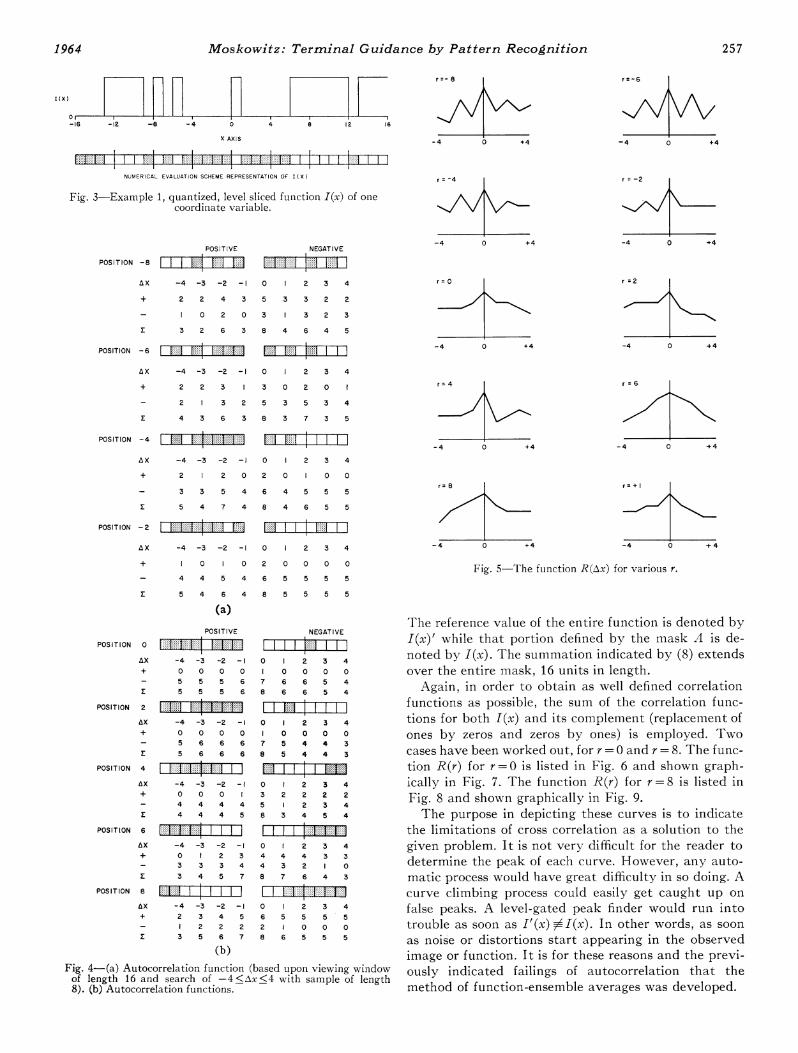
able is shown in Fig. 3. The function 1(x) may assumeonly two values, zero or one, in steps of width w, aninteger multiple of the unit length. The region 6R ex-tends from x =16 to x-= 1-16 and r, the permitteddisplacement of the mask, can take on values betweenx =-8 and x = +8. The mask itself has a length of 16units. (For this one-dimensional case the mask degen-erates to a line segment.) The lower diagram in Fig. 3is a representation of I(x) in such a form that leads tosimple hand computation. By counting unobscuredboxes when a second function, so drawn, is superimposedupon Fig. 3 the integrals represented by (2) and (3)may be evaluated.
B. A utocorrelation
Autocorrelation functions are represented by (2). Be-cause of the unit step form of I(x), integration may bereplaced by summation. For a given r=a, (2) can berewritten,
In order not to violate the restrictions of the mask,I(x +Ax) used in (7) can only have length 8 because Axhas been chosen to have the range -47<AX<4. (Notethat "1" is represented by a white box and "0" by ablack box.) Both I(x) and its negative are used so thatas strong an autocorrelation function as possible isobtained. Fig. 4(a) and 4(b) contain tables of R(Ax) forr= -8, -6, -4, -2, 0, 2, 4, 6 and 8. Fig. 5 containsgraphical representations of the total R(Ax) (indicatedin Fig. 4 by the symbol 1) for the nine listed displace-ments. In addition R(Ax) has been calculated for thedisplacement r= +1. (The data points have been con-nected by straight lines.) The purpose in using thislast point is to indicate that any net which covers lessthan all possible values of r will not necessarily supplya sufficient catalog. If the first nine curves of Fig. 5represent the catalog, then the curve obtained for r= 1can conceivably have been obtained at either the pointr= +1 or r= +7. Fig. 3 also serves for the demonstra-tion of crosscorrelation and the method of function-ensemble averages.
C. Cross Correlation
Eq. (3) may be replaced by the following due to theform of I(x):
(8)X=a+8
R(r) = £ T(x)I'(x + r)1r=a xza-8
where{1
1(x), I'(x) = {0.according to Fig. 3.
Moskowitz: Terminal Guidance by Pattern Recognition
-16 -i2 -8 -4 0 4 8 I2 16
X AXIS
'"' 1 l 1 - - llI '1NUMERICAL EVALUATION SCHEME REPRESENTATION OF I (X
Fig. 3-Example 1, quantized, level sliced function 1(x) of onecoordinate variable.
Fig. 4-(a) Autocorrelation function (based upon viewing windowof length 16 and search of -4<fAx<4 with sample of length8). (b) Autocorrelation functions.
Fig. 5 The function R(Ax) for various r.
The reference value of the entire function is denoted byI(x)' while that portion defined by the mask A is de-noted by I(x). The summation indicated by (8) extendsover the entire mask, 16 units in length.
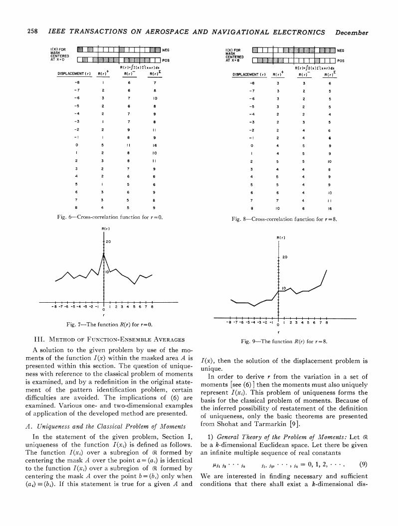
Again, in order to obtain as well defined correlationfunctions as possible, the sum of the correlation func-tions for both I(x) and its complement (replacement ofones by zeros and zeros by ones) is employed. Twocases have been worked out, for r =0 and r = 8. The func-tion R(r) for r =0 is listed in Fig. 6 and shown graph-ically in Fig. 7. The function R(r) for r=8 is listed inFig. 8 and shown graphically in Fig. 9.The purpose in depicting these curves is to indicate
the limitations of cross correlation as a solution to thegiven problem. It is not very difficult for the reader todetermine the peak of each curve. However, any auto-matic process would have great difficulty in so doing. Acurve climbing process could easily get caught up onfalse peaks. A level-gated peak finder would run intotrouble as soon as I'(x) 11(x). In other words, as soonas noise or distortions start appearing in the observedimage or function. It is for these reasons and the previ-ously indicated failings of autocorrelation that themethod of function-ensemble averages was developed.
1964
I1(X H H H
257
POSITION -4 :%::] :;:.:.::: :::::::::I. :-::IE;` E..ilt I
258 IEEE TRANSACTIONS ON AEROSPACE AND NAVIGATIONAL ELECTRONICS December
(X) FOR NEGMASK ..... NGICENTERED
DISPLACEMENT ( r) R( r
-8
-7 2
-6 3
-5 2
-4 2
-3
-2 2
-I
0 5
2
2 3
3 2
4 2
5
6 3
7 3
8 4
R(r)=fI(x)I'(x+r)dxR(r ) ____
6 7
6 8
7
6
7
7
9
8
II
8
8
7
6
5
6
10
8
9
8
9
16
l0
9
8
6
9
I1(X) FOR NEGMASK .. .. .: ECENTEREDAT ...1 POS
R(r)f I(x)I'(x+r)dx
DISPLACEMENT (r) R(r) R(r) R(r)
-8 3 3 6
-7 3 2 5
-6 3 2 5
-5 3 2 5
-4 2 2 4
-3 2 3 5
-2
- I
0
2
3
4
4
4
5
4
5
4
4
5
5
5
4
4
5 5 4
6 6 4
7 7 4
8 10 6
5 8
5 9
6
6
9
9
10
8
9
9
10
I
16
Fig. 6-Cross-correlation function for r=0. Fig. 8 Cross-correlation function for r =8.
R( r)
20
I0
,- ,i-8 -7 -6 -5 -4 -3 -2 -I 2 3 4 5 6 7 80
Fig. 7-The function R(r) for r=O.
III. METHOD OF FUNCTION-ENSEMBLE AVERAGES
A solution to the given problem by use of the mo-ments of the function I(x) within the masked area A ispresented within this section. The question of unique-ness with reference to the classical problem of momentsis examined, and by a redefinition in the original state-ment of the pattern identification problem, certaindifficulties are avoided. The implications of (6) areexamined. Various one- and two-dimensional examplesof application of the developed method are presented.
A. Uniqueness and the Classical Problem of MomentsIn the statement of the given problem, Section I,
uniqueness of the function I(xi) is defined as follows.The function I(xi) over a subregion of 61 formed bycentering the mask A over the point a = (ar) is identicalto the function I(xi) over a subregion of 6R formed bycentering the mask A over the point b = (b,) only when(ai) _ (b). If this statement is true for a given A and
R( r)
20
-8 -7 -6 -5 -4-3-2- 1 2 3 45 6 78
Fig. 9-The function R(r) for r=8.
I(x), then the solution of the displacement problem isunique.
In order to derive r from the variation in a set ofmoments [see (6) ] then the moments must also uniquelyrepresent I(xi). This problem of uniqueness forms thebasis for the classical problem of moments. Because ofthe inferred possibility of restatement of the definitionof uniqueness, only the basic theorems are presentedfrom Shohat and Tarmarkin [91.
1) General Theory of the Problem of Moments: Let 61be a k-dimensional Euclidean space. Let there be givenan infinite multiple sequence of real constants
(9)
We are interested in finding necessary and sufficientconditions that there shall exist a k-dimensional dis-
R1 1ai im i11 1i ia ;it
i
I...Mil j2 . ik il, j27 . 7 ik -'-":
7 )
Moskowitz: Terminal Guidance by Pattern Recognition
tribution function 4 whose spectrum2 is to be containedin a closed set So, given in advance and which is asolution of the "problem of moments"
.7j2 .ik = Xll . . . xkicd b
il, i2 , j = 0,1,2,* . (10)This is called the (So) moment problem. The momentproblem is determined if its solution is unique; other-wise it is indeterminate.To simplify, we shall discuss only the two-dimensional
case k= 2. Let P(xi, x2) be any polynomial in x1, x2 in (R.
P(xl, x2) = Z aibjxlixx2ii
(11)
we have
(19)n
A(P) = E Ii±j(aiaj) - Qn(a)i,j=o
(Hankel quadratic form). Thus a necessary conditionfor the existence of a solution of (16) is that the quad-ratic forms Q74(a), n=O, 1, 2, *. be non-negative. Thiscondition is also sufficient.
Let i6(x) be a solution of (16). Since
Q)Q, (a) = /t (p, 1) = p,'(x)dik
_00
(20)
and if (5') is not reducible to a finite set of points,
where as, bj are real or complex valued constants. Intro-duce the functional,(P) defined by
,(p)= ,Xjaibj. (12)ij
In particular
,u(X1X2j) = 4Ai, (13)
Theorem I: A necessary and sufficient condition that the(25o) moment. problem defined by the sequence ofmoments {lij} shall have a solution is that the func-tional g(p) be (25o) non-negative, that is
,u(p) > 0, whenever p(x1, x2) > 0 on (5o. (14)
A further dimensional reduction yields the Ham-burger moment problem. Here 5o coincides with theaxis of reals. Hence ij=0 for j> 1, so that we have asimple sequence of moments
-n -no n =0O 1 2) . . . (15)and the problem reduces to that of determining a one-dimensional distribution function 46(x) such that
n = 0, 1, 2,In
An = Xnd4l(x)x0
(16)
Thus, it suffices to consider polynomials and functionsof x alone, and to define the functional ,u by
n
Qn(a) = E /i+j(aiaj) > 0,i,j=o
n = 0),1, 2, (21)
provided not all ao, a1, * *, a, are zero, which will beassumed in what follows. From the theory of quadraticforms [10], [11] the conditions (21) are equivalent to
An = In n = 0, 1, 2. (22)
All these results can be stated in:
Theorem II. In order that a Hamburger moment prob-lem
(23)ALn = Xnd4l
shall have a solution, it is necessary that
An= n=0,1,2,- . . (24)
In order that there exists a solution whose spectrum isnot reducible to a finite set of points, it is necessary andsufficient that
An>0 n=0,1,2,*... (25)
In order that there exist a solution whose spectrum con-sists of precisely (k+1) distinct points it is necessaryand sufficient that
The correspondence between 4+(x) of (23) and I(x)of (4) is given byn
pn(x) = E ajxj.j=O
(17)
A(x) = fI(x)dx.Theorem I now states that a necessary and sufficient
condition for the existence of a solution of (16) is that,.u(p) >0, whenever p(x) >0 for all real values of x. Ifwe take for p(x) the particular polynomial
p(x) = (ao + aix + * * + a74x74),2 as real (18)
2 The spectrum 2('i) of a distribution set-function is definedas the set of all points x £E Rk, such that D (G) >0 for every open set Gcontaining x.
(27)
Clearly 41(x) is a bounded nondecreasing function in theinterval (-oo, oo) as required by the problem ofmoments, for I(x) is bounded, contained within thefinite interval 6R and is never negative. Thus except foran arbitrary constant, I(x) is uniquely determined ifthe Hamburger moment problem has a solution.With uniqueness established by conditions (24), Hu
[8] indicates for the two-dimensional moments, the
n
Y(pn)--,ujai,j=o
1964 259
260 IEEE TRANSACTIONS ON AEROSPACE AND NAVIGATIONAL ELECTRONICS December
function I(x1, x2) may be regained from the inverseFourier tranform
10rXI(X1X2) (2ir)2 J00 J x
exp (-iuxl -ivX2)0(U, V)dudv (28)
where q(u, v) is the characteristic function
4)(u, V) = E , M(xmPx2q) - * (29)p=O q=O p! q!
[Note that MJ](x1Px22) is the pth qth moment ofI(x1, x2).]
2) Redefinition of Uniqueness: In order to avoid cer-tain practical difficulties which arise in establishinguniqueness by the procedures derived from the problemof moments, a workable, although possibly more restric-tive, definition is required.
Definition: Given a mask A over a subregion of 6and a set of moments evaluated for each arbitrary dis-placement r, then the displacement is uniquely deter-mined if:
1) For the kth member of the set of moments,M[gk(x)] evaluated about points a and b,
M[gk(X)]a = MA[gk(x)lb, (30)
only if (ar) -(bi). This is sufficient but not neces-sary to establish uniqueness.
2) In general if there exists a set of n moments suchthat for any two arbitrary displacements r = a andr = b, all moments through the nth evaluated abouta and b are identical order for order,
Thus the integration is over the masked area A andthe functions gj are in terms of the coordinates ui of A.Then (6) rewritten in component form is
[Of course (30) can also be rewritten accordingly butsince its meaning is clear, it is left in its present form. IThe functions gj(u) to be employed for the one-
dimensional case may take the form of the power series
(34)
or the trigonometric series
cos Ou, sin u, cos u, sin 2u, cos 2u, , sin nu, cos nu. (35)
For the two-dimensional case the double power series
U 0U20° Ul1U20, U10U21 U12U20 iUltI21, Ui0i22, .,U. U2m (36)
may be used. In this paper Example 1 is evaluatee usingboth (34) and (35) and Example 2 only by use of (36).3The fundamental problem is the numerical deter-
mination of the coefficients aji so that the absolute valueof the error at any point r between the true value of riand that computed by (33) is less than some bound B.(It is also possible to reformulate this condition so thatB is the bound on the rms error or on the averageabsolute error.)
1) The One-Dimensional Case: Consider the one-dimensional problem; if k -1 moments are evaluated atk points (assuming uniqueness) then it is possible towrite a set of k equations in the k unknowns,
a0, ai, a2, . . *, ak (37)
j=01,2,2 * n (31)
only when (a) -(bi). Namely, there is always aleast one moment of the set which is not identicalfor a and b when (a,i) 5 (bi). Now the formationgiven by (6) as a solution to the given problem ofSection I may be tested by numerical evaluationof Example 1, the one-dimensional problem ofFig. 3 and Example 2, the two-dimensional prob-lem of Fig. 13.
B. Solution by MlomentsEq. (6) is somewhat ambiguous in its present form of
notation and so a better statement is required. Definethe jth moment of the distribution I(x) evaluated overthe subregion A centered about the point r with com-ponents (ri) by
M[gj(ui)j7 = j'I(r1 + ui)gj(ui)duj (32)
where
Xi = ri + uidA = lldui.
and solve them accordingly. Uniqueness insures thatthe equation matrix will not be singular. It is possibleto test to see what value of k is required to reduce theerror to below B. It is also of value to determine forthe form of 1(x) employed (unit steps) which of the two,power series or trigonometric series, converges morerapidly. Because 1c(x) is nonanalytic though bounded,one could guess that the latter would be more accuratefor a given number of terms.The approximate (stepwise) representation of the
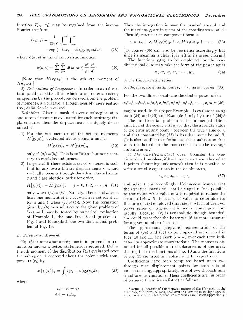
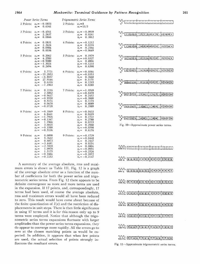
terms of (34) and (35) to be employed are charted inFigs. 10 and 11. The mark ( ) over each term indi-cates its approximate characteristic. The moments ob-tained for all possible unit displacements of the maskA using both the functions of Fig. 10 and the functionsof Fig. 11 are listed in Tables I and II respectively.
Coefficients have been computed based upon twothrough nine displacement points for both sets ofmoments using, appropriately, sets of two through ninesimultaneous equations. These coefficients are (in orderof terms of the series as listed) as follows.
I Actually, because of the stepwise nature of the I(x) used in theexamples, the terms of (34), (35) and (36) are replaced by stepwiseapproximations. Such a procedure simplifies calculation appreciably.
M[gj(x)]a = M[gj(x)]b
0 1 2 3 . . .U) U) U) U) , Un )
Moskowitz: Terminal Guidance by Pattern Recognition
A summary of the average absolute, rms and maxi-mum errors is shown as Table III. Fig. 12 is a graphof the average absolute error as a function of the num-
ber of coefficients for both the power series and trigo-nometric series terms. From Fig. 12 there appears to bedefinite convergence as more and more terms are usedin the expansion. If 17 points, and, correspondingly, 17terms had been used, of course the average absolute,rms and maximum errors would all have been reducedto zero. This result would have come about because ofthe finite quantization of 1(x) and the restriction of dis-placements in unit steps. There is then little significancein using 17 terms and it is for this reason only up to 9terms were employed. Notice that although the trigo-nometric series terms expansions fluctuate with largeramplitudes than the power series terms expansions, theydo appear to converge more rapidly. All the errors go tozero at the chosen matching points as would be ex-
pected. In addition, it appears that when few pointsare used, the actual selection of points strongly in-fluiences the resultant errors.
262 IEEE TRANSACTIONS ON AEROSPACE AND NAVIGATIONAL ELECTRONICS December
TABLE IPOWER SERIES MOMENTS
Term
6 -2.50
-2.25
-4.00
-6.00
-5.50
-4.75
-3.75
-0.50
0.50
3.25
4.00
6.75
7.25
5.50
5.75
5.50
5.00
u2
3.99
9.68
11.24
13.74
12.12
10.18
7.81
8.87
13.37
12.43
15.12
12.43
13.43
10.24
11.93
13.61
15.49 25.26 170.31
TABLE IITRIGONOMETRIC SERIES MOMENTS
Term
sin u
-18
-24
cos 2u
-12
- 4
sin 2u
- 4
0
w sIcos 3u sinl 3u cos 4u
- 6
2
6
13
0
8
sin 4u
0
- 8
-24 0 4 12 3 -8 -8
-22 0 4 13 - 8 -8 8
- 16 - 4 4 - 1 -14 0 16
-12 - 8 12 -14 -13 8 8
-10 - 8 16 -11 5 0 0
- 6 8 16 - 6 3 0 0
0 24 4 -3 8 8 -8
6 20 -16 2 0 -8 - 8
14 12 28 -6 0 0 0
22 12 -28 - 6 0 0 0
26 - 4 -16 _ 9 8 8 - 8
28 -24 4 7 11 -8 - 8
30 - 8 16 10 0 0 0
28 16 12 -4 -3 8 -8
24 28 4 12 3 0 -16
Displacement
-8
-7
-6
-5
-4
-3
-2
1
0
2
3
4
5
6
7
8
7
7
7
6
5
4
4
S
5
6
6
7
7
8
9
10
U3
- 3.07
1.35
- 6.45
-15.76
-15.91
-14.74
-11.96
0.81
2.0
11.36
10.57
19.28
19.12
10.29
11.53
11.51
10.16
U5
- 4.08
20.14
-11.68
-51.71
-54.00
-50.71
-40.36
12.56
8.82
39.60
27.04
59.83
59.31
25.29
36.32
36.32
4.14
24.88
27.32
38.26
33.94
29.14
22.38
27.88
46.44
39.82
48.94
34.20
35.20
20.70
29.94
38.58
47.88
u6
5.2
80.41
75.63
120.48
109.93
98.70
76.57
97.54
169.09
134.79
172.93
110.09
110.93
49.93
91.80
128.42
- 5.78
105.02
- 22.87
-183.20
- 191.63
-182.20
-145.96
72.94
33.21
145.09
72.15
201.03
200.93
68.53
133.91
133.91
68.53
U8
7.16
288.71
208.41
401.26
376.51
350.96
282.75
349.86
625.55
457.45
631.51
376.61
377.51
126.57
314.36
438.86
626.65
Displace-ment
-8
-7
-6
-5
-4
-3
-2
-1
0
1
2
3
4
5
6
7
8
cos Ou
6
7
7
7
6
5
4
4
5
5
6
6
7
7
8
9
10
cos u
+22
+ 6
- 2
-12
-12
-10- 6
-10
-18
-16
-22
-14
-12
- 2
2
6
8
=1 ..l l.. 1..1-
II ~ _
I1I
11 1.
11 I1 -
Moskowitz: Terminal Guidance by Pattern Recognition
TABLE IIIERRORS FOR EXAMPLE 1
TABLE OF ERRORS
Num- Power Series Terms Trigonometric Series Termsber of
cients Average RMS Maximum Average RMS Maximum
2 1.91 2.81 5.90 44.78 61.77 151.33
3 5.12 6.41 10.48 2.69 3.22 5.56
4 0.91 1.44 4.10 1.44 2.13 6.00
5 1.46 2.13 5.48 6.69 9.33 21.58
6 3.92 5.68 12.05 0.93 1.53 3.56
7 1.36 2.21 5.96 1.83 2.57 5.49
8 1.20 1.94 5.69 2.62 4.53 10.67
9 1.24 2.37 7.40 0.63 1.15 3.07
a:0
0
a:
3w
0
mLi
0
I TRIGONOMETRIC SERIESTERMS
POWER SERIES -
TERM
where
M [gj(ul, U2) ] rl,,
= LI(ri + ul, r2 + u2)gj(Ul, u2)du,du2. (40)
Thus it is necessary to solve for one set of coefficientsfor the displacement component r1 and another for thedisplacement component r2. Arbitrarily, it has been de-cided to use power series terms through the third power,namely,
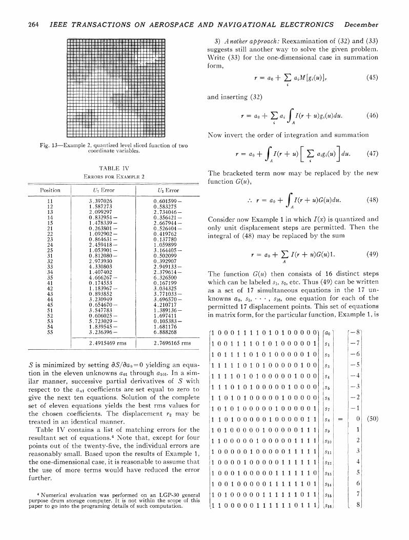
However, instead of using just eleven displacementpoints to obtain the sets of eleven coefficients implied by(38), (39) and (41), twenty-five maybe employed if root-mean-square curve fitting techniques are resorted to inorder to treat the excess of data. Example 2, a functionof the two variables xi, x2, is shown as Fig. 13. It isquantized into a grid 32 bits by 32 bits, each havingthe value zero or unity. Coordinate axes are establishedat the center of the grid and form the reference for thedisplacements ri, r2 of the mask A. The mask A is agrid 16 bits by 16 bits again with coordinate axes u1, u2established at its center. Displacements in the range-8 < xi < 8 are permitted. [If twenty-five evenly spaceddisplacements are to be employed for purposes of nu-merical computation, then r1 and r2 are tested withvalues of -8, -4, 0, 4 and 8. Using the ordering ofindices of matrix notation, the displacement r1= -8,r2=8, corresponding to the position in the upper leftcorner, is labeled "11." The center position, for instance(r1= r2= 0), has the label "33. "]For the matching process the moments obtained for
the various positions are employed in evaluating thecoefficients of (38) and (39) by the method of leastsquares. Eq. (38), by way of example, can be expressedmore compactly
10
ri(ij) = a01 = E anlM[gn(u)]7(i1)n=l
(42)
2 3 4 5 6 7 8 9 10
NUMBER OF COEFFICIENTS
Fig. 12-Error curves for Example 1.
2) The Two-Dimensional Case: If both I is a functionof two coordinates I(xi, x2) and displacements in twodimensions r1 and r2 are permitted, then (33) yields thepair of equations
where ri(ij) is the displacement at the ith jth positionof the reference function I(xi, x2) and M[gn (u) ]r(ij)the corresponding moment for the at, coefficient.The sum of the squares S of the deviations is repre-
sented by10 \2
S= ,r(ij) - aol + , anlM[gn(u)]r (i))j (43)ti n=1
The partial derivative of S with respect to the coefficienta0 is
as = _2 [r1(ij)cdao ii
-a0 (a01 + E a1(- aol + E an1M[gn(U)>.(i))] (44)
1964 263
(39)
264 IEEE TRANSACTIONS ON AEROSPACE AND NAVIGATIONAL ELECTRONICS December
3) Another approach: Reexamination of (32) and (33)suggests still another way to solve the given problem.Write (33) for the one-dimensional case in summationform,
r = ao+ E aiM[gi()] (45)
and inserting (32)
r = ao + E ai I(r +u)g(u)du.iA
(46)
Now invert the order of integration and summationFig. 13-Example 2, quantized level sliced function of two
The bracketed term now may be replaced by the newfunction G(u),
.. r = ao+ JI(r +u)G(u)du. (48)
Consider now Example 1 in which I(x) is quantized andonly unit displacement steps are permitted. Then theintegral of (48) may be replaced by the sum
r = ao + E I(r + u)G(u)1.A
(49)
The function G(u) then consists of 16 distinct stepswhich can be labeled s1, S2, etc. Thus (49) can be writtenas a set of 17 simultaneous equations in the 17 un-knowns ao, si, * , s56, one equation for each of thepermitted 17 displacement points. This set of equationsin matrix form, for the particular function, Example 1, is
i10 1 111 0 1 0 1 0 0 0 0 0 1 0S is minimized by setting &S/Oao =0 yielding an equa-tion in the eleven unknowns ao1 through a10l. In a sim-ilar manner, successive partial derivatives of S withrespect to the a,, coefficients are set equal to zero togive the next ten equations. Solution of the completeset of eleven equations yields the best rms values forthe chosen coefficients. The displacement r2 may betreated in an identical manner.
Table IV contains a list of matching errors for theresultant set of equations.4 Note that, except for fourpoints out of the twenty-five, the individual errors arereasonably small. Based upon the results of Example 1,the one-dimensional case, it is reasonable to assume thatthe use of more terms would have reduced the errorfurther.
4 Numerical evaluation was performed on an LGP-30 generalpurpose drum storage computer. It is not within the scope of thispaper to go into the programing details of such computation.
11111010100000100
itI1 1 0 1 0 1 0 0 0 0 0 1 0 0 0
11 1 0 1 0 1 00000 1 0000
1 1 0 1 0 1 0 0 0 0 0 1 0 0 0 0 0
1 0 1 0 1 0 0 0 0 0 1 0 0 0 0 0 1
l I 0 1 0 0 0 0 0 1 0 0 0 0 0 1 1
1 0 1 0 0 0 0 0 1 0 0 0 0 0 1 1
11 0 0 0 0 0 1 00 0 0 0 1 1 1 1
110 0 0 0 1 0 0 0 0 0 1 1 11 1
i1 00010000011 1 1 11
1100 100000 1 1 1 1 1 0
11
1l
101t11
I
0100000 1 1 1 1 1 10111
1 0 0 0 0 0 11 1 1 1 1 0 1 1 1
ao )
Si1S2
S3
SsI
S4 I
S51
l
jSilS13
Is
Sg
512
S15S
S16
-61-51
-41:-3j
-11 51
21
341
4
i1
1672J
(50)
Moskowitz: Terminal Guidance by Pattern Recognition
Solution of (50) yields
aO = - 5.748 S6 = 0.664
S1 = 1.017 S7 = 0.504
S2 = 2.471 S8 = - 2.555
S3 = 1.067 S9 = 1.824
54 = - 3.261 Sio= 3.546
S5 = - 2.706 Si' = 4.370
Use of the above function, G(u) indimensional function I(x) shown in
S12 = 1.857
s13 = -0.605
S14 = 1.345s1 = 3.496
S16 = 1.992
(49) for the one-
Fig. 3 gives an
exact solution for r, the displacement of the mask withrespect to the reference coordinates of JR for each of thequantized displacements r = x, x =-8, -7, * + 7,+8. Thus a solution to the given problem is obtainedwhich requires neither a catalog of functions (as withautocorrelation) nor a search and logical decision proc-
ess (as with cross correlation).
IV. CONCLUSIONSThis paper has investigated various solutions to the
problem given in Section I. Autocorrelation and cross
correlation, both conventional approaches, have beendiscussed and their limitations indicated. An originalsolution, calledl the method of function-ensemble aver-
ages, was presented, its relation to the classical problemof moments indicated and demonstration examplessolved by its application.The method of function-ensemble averages was
shown by means of numerical examples to yield a solu-tion to the given problem with bounded error. By choiceof technique employed for the numerical evaluation of
a set of coefficients this bound may be made arbitrarilysmall. If quantized displacements are permitted, it ispossible to obtain zero error, or exact matching, overthe entire given region and range of displacement. Theexamples presented covered both one- and two-dimen-sional problems. The five-dimensional problem, that ofterminal guidance for reentering ballistic body, can alsobe solved by the method of function-ensemble averages.An appropriate grouping of the basic equations will thenyield this solution. Feasible approaches to mechaniza-tion are implicitly contained within the given formula-tion.
REFERENCES[1] M. Minsky, "Steps toward artificial intelligence," PROC. IRE,
vol. 49, pp. 8-30; January, 1961.[2] J. K. Hawkins, "Self-organizing systems-a review and com-
mentary," PROC. IRE, vol. 49, p. 31-48; January, 1961.[3] F. Rosenblatt, "The Perceptron," Cornell Aeronautical Lab.,
Ithaca, N. Y. Report No. VG-1196-G-1; January, 1958.[4] J. A. Fitzmaurice, "Final Report on Pattern Recognition
[5] L. P. Horwitz and G. L. Shelton, Jr., "Pattern recognition usingautocorrelation," PROC. IRE, vol. 49, pp. 175-185; January,1961.
[6] J. P. Martino, "A New Class of Target-Recognition Seekers forMissile Terminal Guidance," USAF, WPAFB, Dayton, Ohio,WADC Technical Note No. 57-265; July, 1957.
[7] M.-K. Hu, "Pattern recognition by moment invariants" PROC.IRE (Correspondence), vol. 49, p. 1428; September, 1961.
[8] "Visual pattern recognition by moment invariants,"IRE TRANS. ON INFORMATION THEORY, vol. IT-8, p. 179-187;February, 1962.
[9] J. A. Shohat and J. D. Tarmarkin, "The Problem of Moments,"Mathematical Surveys, American Mathematical Society, NewYork,N.Y.; 1943.
[10] L. Mirsky, "An Introduction to Linear Algebra," OxfordUniversity Press, New York, N. Y.; 1955.
[11] H. Schwerdtfeger, "Introduction to Linear Algebra and theTheory of Matrices," P. Noordhoff N.V., Groningen, Holland;1950.