D O C U M E N T O D E T R A B A J O

Instituto de EconomíaTESIS d

e MA

GÍSTER

I N S T I T U T O D E E C O N O M Í A

w w w . e c o n o m i a . p u c . c l

A Robust Macroeconomic Model for Asset Pricing

David Ruiz G.

2011

A Robust Macroeconomic Model for Asset Pricing

David Ruiz G.∗

October 19, 2011

Abstract

In a continuous-time model with two agents, include knightian uncertainty as an additional fea-

ture to heterogeneity on elasticity of intertemporal substitution (EIS) and limited market participation

(LP), makes stockholder more precautious than non-stockholders. This provides an endogenous source

of heterogeneity among agents and, potentially, a theoretical explanation for the required smoothness

of consumption growth to match empirical moments observed on data. However, in a partial equilib-

rium setting, where agents have Epstein-Zin preferences, consumption is determined by time-preference

parameters, while knightian uncertainty increases total effective risk perceived by both agents, affecting

only optimal portfolio strategies. Also, this paper shows the strong implications of robust decision-makers

when they fear about model misspecification.

∗Pontificia Universidad Catolica de Chile. Email: duruiz@uc.cl

1

1 Introduction

Knight’s (1929) distinction between uncertainty and risk in economic environments, and Ellsberg-type

(1961) experiments on the behavior of economic agents has promoted a large and growing research agenda

with significant economic implications. One of the most important consequence relates to the traditional

approach of rational expectation theory that, by imposing equality between agent’s subjective probabilities

and those arising from the economic model containing those agents, creates a three-way cross-equation re-

striction between agents beliefs, the economic environment, and the econometrician modeling the economic

phenomenon. As Hansen and Sargent (2010) argue, when agents doubt about the underlying data generating

process, they only have an approximate model. View models as approximations requires, somehow, refor-

mulate the common models condition imposed by rational expectation. In this sense, what Ellsberg (1961)

paradox suggests is that agents preferences are not only influenced by risk aversion, but also by uncertainty

aversion (i.e. economic agents fear that the data are generated by an unknown disturbance of approximate

model). Uncertainty aversion represents a preference for knowing probabilities over having to form them

subjectively based on imprecise information.

Until the seminal paper of Epstein and Wang (1994), where knightian uncertainty leads to an indeterminate

equilibrium of asset prices, financial economics literature answered to the question about the optimal port-

folio and the optimal consumption plan under strong assumptions on agent’s beliefs. At first, indifference

between risk and uncertainty in the sense of Knight, a rigid specification on preference parameters, and “the

representative agent” assumption were the main culprits that led to well-known puzzles in consumption-

based asset pricing models. For example, two of the most famous puzzles are the Equity Premium Puzzle

(Mehra and Prescott (1985)) and the Risk-free Rate Puzzle (Weil (1989)). Although, since 1990s, the efforts

of many works focused on identifying the fundamental characteristics of financial markets1, it remains an

open question the economic relationship between asset prices, interest rates and macroeconomic variables,

specially its relationship with the consumption growth.

This paper attempts to provide a theoretical explanation for the poor empirical and economic performance

of standard models that relates asset prices, interest rates and consumption growth. I introduce a two-

agent model in continuos time for an exchange economy, where prices are given and solve for optimal

consumption plan and portfolio strategies. I consider key features of financial markets in order to account

for the three main criticisms of asset prices models presented above, namely: limited participation (LP),

heterogeneity on elasticity of intertemporal substitution (EIS), and knightian uncertainty. I adopt Hansen,

Sargent, Turmuhambetova, and Williams’s (2006) penalty problem approach for modeling robust control

problems on fixed probability spaces where both agents know an approximate model of the underlying data

generating process, and alternative models are represented as martingale “preference shocks”.

Related to this work is Guvenen (2009), who presents an explicit economic mechanism that accounts for the

poor performance between asset prices and macroeconomic variables of previous models. His real business

cycle model is consistent with some key features of asset prices, such as a high equity premium, relatively

smooth interest rates, pro-cyclical stock prices, and countercyclical variation in the equity premium, its

volatility, and in Sharpe ratio. However, when it comes to business cycle performance, the model’s progress

has been more limited: consumption is too volatile compared to data, whereas investment is still too smooth.

1Campbell (2003) suggests that to make sense of asset prices behavior one need a model in which the market price of

risk is high, time-varying, and correlated with the state of the economy (for example models with habit formation in utility,

heterogeneous investors, and irrational expectations).

2

As a previous step, in this paper I explore if knightian uncertainty provides an endogenous source of hetero-

geneity among agents and, potentially, a theoretical explanation for the required smoothness of consumption

growth to match empirical moments observed on data. In particular, on Guvenen’s work there is no mean-

ingful distinction between risk and uncertainty, in the sense that economic agents can represent all available

information on a unique probability distribution. I pretend to consider an economic environment where

information is too imprecise to be summarized on a unique probability measure and agents only know an

approximate model of the underlying data generating process. However, in a partial equilibrium setting,

where agents have Epstein-Zin preferences, consumption is determined by time-preference parameters, while

knightian uncertainty increases total effective risk perceived by both agents, affecting only optimal portfolio

strategies.

The following subsection, presents the main hypothesis of the paper and the economic mechanism behind

it, and also discusses related literature. Section II contains main results of the theoretical approach for the

benchmark case, and under knightian uncertainty. Section III presents empirical results for three cases of

utility specifications given as extreme cases of Epstein-Zin recursive utility. Section IV concludes. Details

about proof of propositions and explicit solutions are presented in the Appendix A. Appendix B describes

three important topics related to knightian uncertainty, namely observational equivalence, dynamic consis-

tency and learning, which helps to motivate the importance of considering ambiguity scenarios on financial

and macroeconomic models.

1.1 Hypothesis and Related Literature

In a general equilibrium setting, the presence of knightian uncertainty on agents behavior should reinforce

Guvenen’s (2009) results, consistent with high equity premium, low and smooth interest rates, and smoother

consumption growth. In particular, limited stock market participation and heterogeneity in the EIS are

both introduced as exogenous characteristics of the economic environment which, combined with rational

expectation behavior, generates Guvenen’s (2009) results. However, my argument is that those results are

biased (specially on macroeconomic variables). Providing agents with the probability measure makes rational

expectation an exogenous restriction over what agents know about the stochastic environment. By equating

subjective with objective probabilities, rational expectation forces that agents seek for decision rules that

only perform well under that, and only that, probability measure.

On the other hand, knightian uncertainty relates to how agents make decisions with imprecise or inaccurate

information. This approach permits to disentangle risk aversion from uncertainty aversion by representing

a preference for knowing probabilities over having to form them subjectively, something that is not allowed

by rational expectation theory. From my point of view, this distinction is significant in terms of what we

assume about agents behavior. Agent’s fear to model misspecification promotes robust decision-making,

in the sense that agents choose decision rules that not only performs optimally when the underlying data

generating process holds exactly, but also performs reasonably well if there is some form of model misspec-

ification, and unambiguously will perform better than the traditional approach of decision-making under

model misspecification.

3

1.1.1 Standard Expected Utility Models, Limited Participation, and Heterogeneity in EIS.

Let’s consider two well understood examples related to puzzling evidence of consumption-based models of

asset prices.

• Example 1. The Equity Premium Puzzle. Mehra and Prescott (1985). Consider an economy

where standard assumptions of representative agent holds (i.e. CRRA preference, complete markets

and returns and consumption growth distributed jointly log-normal). Assuming that Euler equation

which determined stock and bond choices hold with equality, the equity premium can be decomposed

as:

E(Rep)

std(Rep)≈ α× std(∆c)× corr(∆c,Rep)

From post-war U.S. data, Sharpe ratio for equity premium is E(Rep)std(Rep) ≈ 0.4, the standard devia-

tion of (log-) consumption growth std(∆c) < 2% and its correlation with the excess of return is

corr(∆c,Rep) < 1, it implies that RRA : α ≈ 40 which is excessively high risk aversion to rationalize

the observed premium, which also will have strong implications for decision-making.

• Example 2. Risk-free Rate Puzzle. Weil (1989). The implied equilibrium relation for risk-free

rate from the previous assumption can be approximated by three fundamental components of saving,

namely, time preference, intertemporal substitution and growth, and precautionary savings:

E(Rf ) ≈ −ln(β) + αE(∆c)− α2

2var(∆c)

Again, from post-war U.S. data, subjective time discount rate is between 0 < β < 1, average of (log-)

consumption growth is E(∆c) = 1.5% per year, and from previous result α ≤ 40, then it implies an

interest rate of E(Rf ) ≈ 60% per year, which is too high for the realistic average interest rate of

3%. One reasonable explanation for this puzzle is as follows: Households are extremely unwilling to

substitute consumption over time, so, they want to transfer more consumption to today, to achieve a

flat consumption profile. In equilibrium, this can not be done, which simply pushes up the risk free

rate.

Both examples show the effects of the assumptions of standard models of expected utility in the equilibrium

relationships between the risk premium, risk-free rate and consumption growth. The main criticism of

these models are related to the poor empirical performance and its contradiction to dynamic macroeconomic

literature, a point presented by Guvenen (2006). On the one hand, macroeconomic literature typically uses a

value closed to one for EIS, which presumably is more consistent with U.S. aggregate data. However, a well

documented evidence since the 1980s shows that consumption growth is completely insensitive to changes in

interest rates, hence, EIS is very closed to zero (Hansen and Singleton (1983); Mehra and Prescott (1985);

Hall (1988); reported very low estimates for EIS with standard models.)

There are three reasons to explain this contradicting evidence2: First, standard expected additive utility

models assumes rigid specifications to represents preferences; second, representative agent models assumes

that average consumer is identical to average investor; and finally, assumes homogeneous agent’s beliefs or

the existence of a unique probability distribution.

2The first two of them are well documented in Guvenen (2006)

4

To account for a rigid specification of preferences, Epstein and Zin (1989, 1991) presents a testable model

based on preference that allows a clear separation between risk aversion attitudes and intertemporal sub-

stitution. In their empirical version, they find that the EIS is less than one, and consumers prefers a late

resolution of uncertainty3 (α > ρ), in the sense of Krepts and Porteus (1978). Closer to the present paper

is Duffie and Epstein (1992a, b), which presents the continuous-time analogue of the Epstein-Zin’s class of

recursive utility4.

Secondly, Guvenen (2006, 2009) establishes that the apparent inconsistency between the dynamic macroe-

conomic literature and empirical findings is a consequence of the “representative agent” perspective. This

models assumes that average consumer is identical to average investor. However, two important empirical

observations suggest that they are very different. First, Poterba et al. (1995) reports that until the 1990s

more than two-thirds of U.S. households did not own any stocks at all, while the richest 1% held 48% of all

stocks. In the same way, the Survey of Consumer Finances, reports that the participation rate is 88.84%

among households with wealth above the median, and only 15.21% for those with wealth below it5. Put

differently, an average investor owns 29.3 times the productive wealth of an average consumer, but consumes

only 1.7 times more. In second place, Mankiw and Zeldes (1991) reports an extreme skewness on wealth

distribution in U.S. data, but consumption turns out to be much more evenly distributed across households.

In particular, for U.S. data, the richest 20% own 83% of net worth and 95% of financial asssets, but account

for only about 30% of aggregate consumption.

In addition, as proposed by Guvenen (2009) and Gomes and Michaelides (2007), new evidence of the 1990s

suggest that non-stockholders have an EIS close to zero, while stockholder have a higher EIS (i.e. Blundell,

Browning and Meghir (1994), and Malloy, Moskowitz, and Vissing-Jørgensen (2006)). One theoretical ex-

planation for these results was provided by Browning and Crossley (2000). They show that the two effects

about changes in consumption to temporary income falls suggested in the literature, namely, the conventional

Marshallian effect and that agents will cut by a greater amount consumption of goods that have a high EIS,

are two sides of the same coin: Luxury goods tend also to have high intertemporal substitution elasticities,

consequently, the EIS (with respect to total consumption) increases with wealth.

To account for these stylized facts, Guvenen (2006, 2009) presents a model with two sources of heterogeneity:

limited participation in stock market and heterogeneity on EIS. When considering limited participation in

stock market, Guvenen (2009) realizes the implicit assumption on representative agents models, namely,

that average consumer is identical to average investor. Through the use of Epstein-Zin preferences, which

disentangle risk aversion from EIS, Guvenen (2009) is able to consider agents who differ in their EIS without

restricting their risk aversion attitudes.

The main argument of his approach is as follows: limited participation in stock market, while restricting

at the majority of population with low-EIS, creates substantial wealth inequality while maintaining con-

sumption evenly distributed, making average consumer different from average investor, as observed in U.S.

data. By this way, properties of aggregate variables directly linked to wealth are almost entirely determined

by stockholders with high-EIS who own virtually all the wealth of the economy. On the other hand, while

non-stockholders are able to trade in bond markets at a risk-free rate, aggregate consumption, and hence

Euler equations, not only reveal the low EIS of the majority of the population, but also, non-stockholders

preferences influence the properties of financial variables. Therefore, contradictions noted above are the

3More about the relation between α, ρ and the time of resolution of uncertainty, will be provide in the next section.4More about Duffie and Epstein (1992) will be provide in the next section.5The median wealth for stockholders is $ 154,600, while the median wealth for nonstockholders is $ 7,300.

5

results of estimating EIS from Euler equations that captures an average of individual elasticities from pop-

ulation, where the majority are precisely non-stockholders with low EIS; this is inappropriate for a correct

measurement of elasticities associated to wealth-related variables, as saving, investment, and output.

However, Laibson et al. (1998) and Guvenen (2006) discuss the empirical observation about the relationship

between limited participation and heterogeneity in the EIS. When facing with two agents with the same EIS

that only differ on their wealth position, if one of them is restricted to borrow, typically the poor agent, their

consumption will be related almost one-to-one with income, and will not respond to interest rate variation,

unlike the consumption of the wealthier agent, who can trade freely in the stock market. When elasticities

are estimated from consumption data, poor agent will appear as having a lower EIS than the stockholder.

If true, there may not be any significant heterogeneity in the EIS at first. This observation make place to

the question about how much account limited participation and heterogeneity in EIS on observed data.

It is well documented that one of the main difference between groups is that the observed ratio between

consumption growth variances is approximately σ2(∆ch)σ2(∆cn) ≈ 2 − 4 across different consumption measures for

U.S. data. At first, this is very contradicting. Given that stockholders are much more wealthier and have

access to stock markets, and oppositely, low-income non-stockholders face higher state and income risk, one

might expect that consumption of the former group be much more smoother than that of the latter: because

low-income non-stockholders cannot self-insure, they are borrowed constrained most of the time. Therefore,

its consumption should be one-to-one to their income and hence will be very volatile.

In fact, Guvenen (2006) shows that when there is no difference between agents preference (ρh = ρn) the

ratio of variances is less than one. But, when EIS of non-stockholders is relatively lower than stockholders,

this ratio changes significantly, reaching almost four times. What Guvenen (2006) suggests is that limited

participation alone does not account for this empirical fact. Is the strong desire of non-stockholders for

smooth consumption that make them need the bond market much more than stockholders, driving interest

rates down, increasing equity premium and reconcile the empirical evidence.

The literature recognizes mainly two economic mechanisms that can generate high equity premium on

these incomplete market contexts, as presented above. One is Saito (1995) and Basak and Couco (1998),

who stressed the role of (exogenous) limited participation as a channel to leverage stockholder’s portfolio.

As Guvenen (2009), and other critics to this mechanism recognizes, it only works quantitatively if interest

payments made from stockholders to non-stockhodlers are substantial, which implies that non-stockholders

own a large fraction of aggregate wealth, something that is not observed on U.S. data.

Alternatively, Guven (2009) proposed a different mechanism than previous models, which avoids the coun-

terfactual effects.This results from the interaction of three factors:

First, non-stockholders receive stochastic labor income every period and trade in the bond

market to smooth the fluctuations in their consumption. Second, because of their low EIS,

non-stockholders have a stronger desire for consumption smoothing and therefore need the bond

market much more than stockholders (who have a higher EIS and an additional asset for con-

sumption smoothing purposes). However, and third, since the source of risk is aggregate, the

bond market cannot eliminate this risk and merely reallocates it across agents.

In equilibrium, stockholders make payments to non-stockholders in a countercyclical fashion, which serves

to smooth consumption of non-stockholders and amplifies the volatility of stockholders, who then demand

6

a large premium for holding aggregate risk, premium that, by the same mechanism, is a countercyclical

one. Finally, even that the question about which of these two mechanism proposed previously operates is

an empirical one, in my opinion the one proposed by Guvenen had much economic sense in identifying the

relevant margins between consumption smoothing and investment decisions considering the trade-off between

heterogeneous EIS and (exogenous) differences in opportunity sets among agents. So, even though I do not

have references that test both hypotheses, I will adopt Guvenen’s approach.

1.1.2 Hypothesis: The Effects of Knightian Uncertainty

My hypothesis relies on considering a meaningful distinction between risk aversion and uncertainty aversion

when agents can not summarized all available information on a unique probability measure, a way of relaxing

the homogeneous beliefs and existence of a unique prior assumptions from the previous models.

In the present context, when agents fear about model misspecification, they prefer decision-rules that

perform well across a variety of models. Non-stockholders choose a consumption plan that maximizes their

current utility process selecting endogenously the probability distribution that generates the lowest expected

value of future continuation utility. By the same way, stockholders choose not only a consumption plan but

also an optimal portfolio strategy on equity holdings.

As both agents face different investment opportunities sets (i.e. while non-stockholders face risk and

uncertainty from state variables, stockholders face further risk and uncertainty from asset prices) they will

choose different probability measures. Given that both agents are endowed with a common approximate

model, when selecting their probability distribution they must incur in a change of probability measure. The

change of measure from the approximate model to the lower-bound of the admissible set of expected values

change the instantaneous mean rate of the stochastic processes but not the volatility of them, at least in pure

Markovian diffusion settings. In other words, after a change of measure each agent considers the same set

of path generated by the approximate model (and the underlying probability space), but they endogenously

change the likelihood of them. As non-stockholders are only concerned about the stochastic process of the

state variable they will assign more probabilities in worst-case scenarios of just the state variables. On the

other hand, stockholders puts more probabilities in worst-case scenarios from both, state variables and asset

prices. This makes that stockholders be much more precautionary than non-stockholders when choosing

they decision rules. In summary, while ex ante both agents are endowed with a homogeneous approximate

model, in equilibrium, knightian uncertainty introduced endogenously a new source of heterogeneity between

agents, namely, stockholders are extremely more precautionary than non-stockholders.

In a partial equilibrium setting, where agents are competitive price takers, and because both agents do not

know the true probability distribution, there is an extra incentive to substitute future consumption for current

consumption or, alternative, for a strong position on the risk-less asset. However, due to heterogeneity in

the endogenous probability distribution, stockholders have an extra reason for precautionary savings and

consumption smoothing. Moreover, because of their low EIS, non-stockholders need the bond market much

more than stockholder (who have a higher EIS and an additional asset for consumption smoothing purposes).

In equilibrium, it must be true that stockholders decrease their share of optimal portfolio allocation with

the amount of ambiguity in the economy, and moreover, while consumption growth volatility for both agents

should decrease, the extra precautionary motive of stockholders should reduce consumption growth volatility

even more.

7

2 The Model

I consider a two-agent continuous-time consumption-based asset pricing model in a partial equilibrium

setting, where prices are given and I solve for optimal consumption and portfolio strategy (see Cox, Ingersoll

and Ross (1977, 1985), Lucas (1978) and Breeden (1979)). The main objective of this paper is to study

the effect of heterogeneous knightian uncertainty on optimal consumption plans, as an additional feature

to those proposed by Guvenen (2009), and provide theoretical explanations for the required smoothness in

consumption growth to match empirical moments observed on data.

I present a benchmark problem, where agents had no concern for knigthian uncertainty, and provide solutions

for different utility specifications in terms of partial differential equations (PDE). Then, I consider the same

economic context than benchmark case, however, agents can not summarized all available information into

a unique probability measure, which motivates the presence of agents with preference for robustness, i.e.

agents fear about model misspecification. I provide solutions for different utility specifications in terms of

PDE’s. However, when prices follows an affine structure of the state variable, there is no closed-form solution

to PDE’s resulting from robust control problem. For this, I consider asymptotic expansions to obtain local

approximations around a solution with known closed-form.

2.1 A Benchmark Control Problem.

Let Bt : t ≥ 0 denote a n-dimensional standard brownian motion that induce a Wiener measure on an

underlying probability space (Ω,F, P 0). For the rest of this section, let Ft : t ≥ 0 denote the associated

filtration generated by this brownian motion, satisfying the usual conditions of completeness and right-

continuity, representing the evolution of the relevant uncertainty for the economy. Moreover, let C = (0,∞)

denote the consumption space and C be the class of feasible C-valued consumption processes c = ct : t ≥ 0.

Households.

As in Guvenen (2009), the economy is populated by two types of agents who lived forever. There is no

population growth and it is normalized to unity. Let µ ∈ [0, 1] denote the measure of the second type of

agents (“stockholders”) and (1− µ) ∈ [0, 1] denote the measure of the first type (“non-stockholders”).

It is assumed that there is a single good that, in equilibrium, must be consumed by both individuals.

Stockholders receives an endowment, and they are able to trade two kind of assets in this economy: risky

assets, entitling the owner to the risky endowment (the dividend), and a risk-less asset. Non-stockholders,

are able to trade only the risk-less asset. As in Guvenen (2009), in these incomplete market context, the

difference between the two agents is in their investment opportunity sets.

Financial Markets.

It is assumed that there exist a (d×1) vector of state variables xt : t ≥ 0, that with time, describe the state

of the world, an (n × 1) vector of asset prices, and each asset is associated with a dividend or endowment

process. Assuming that the state vector follows a continuous-time Markov diffusion process of the Ito type

8

then, the risk-free bond, asset prices and dividends follows:

dxt = µx(xt)dt+ σx(xt)′dBt (1)

dMt = Mtr(xt)dt

dSitSit

=

(µSi(xt)−

Dit

Sit

)dt+ σSi(xt)

′dBt for each asset

dDit

Di= µDi(xt)dt+ σDi(xt)

′dBt for each asset

where µl(·, ·) is the instantaneous expected mean rate of change, σl(·, ·) is the instantaneous standard devi-

ation of that rate of change for l ∈ x, S,D, and Bt : t ≥ 0 denote a n-dimensional standard brownian

motion that induce a Wiener measure on an underlying probability space (Ω,F, P 0). The total return for

each risky asset, is given by:

dSit +Ditdt

Sit= µSidt+ σSi(xt)

′dBt (2)

The expected return on security i is determined by the absence-of-arbitrage condition

µSi(xt) = r(xt) + σSi(xt)′λ(xt) (3)

where the instantaneous expected mean rate of change of asset i must be equal to the instantaneous rate

of return of the risk-less asset plus the risk premium of that asset, adjusted by its instantaneous standard

deviation. A portfolio can be characterized by a vector of weights, π, for the risky assets and a weight π0

for the money-market account such that∑n

1=0 πi = 1. Let ΣS be the matrix whose i− th column is σSi and

define µS = (µS1 , ..., µSn) and π = (π1, ..., πn). The value of a portfolio evolves as follows:

dφtφt

= π0dMt

Mt+

n∑i=1

πidSi +Dit

Si= µφ(xt)

′dt+ σφ(xt)

′dBt (4)

µφ = π0r(xt) + µS(xt)′π = r(xt) + λ(xt)

′σφ(xt)

σφ = ΣSπ

Let W k denote the financial wealth for agent k = h, n, whose dynamic is represented by:

dW kt = W k

t

dφktφkt− ckt dt (5)

dW kt = (W k

t (r(xt) + (πk)′ΣSλ(xt))− ckt )dt+W k

t (πk)′ΣSdBt

by imposing that πn = 0, results on wealth dynamic for non-stockholder.

Preference.

On the benchmark case, we assume that both agents know the true probability measure P 0, so there is no

meaningful distinction between risk and uncertainty, in the sense of Knight.

I consider investors with recursive preferences of the Epstein-Zin type. As in Duffie and Epstein (1992 a,

b), it will be necessary to define a recursive utility function for a general class of preference; introduce an

aggregator functional for the particular case of Epstein-Zin; and finally, formulate the dynamic programming

equation for each agent.

9

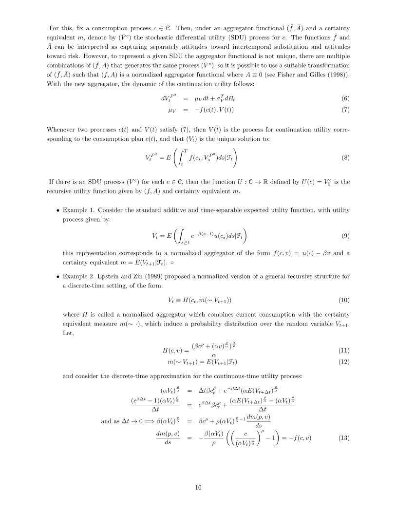
For this, fix a consumption process c ∈ C. Then, under an aggregator functional (f , A) and a certainty

equivalent m, denote by (V c) the stochastic differential utility (SDU) process for c. The functions f and

A can be interpreted as capturing separately attitudes toward intertemporal substitution and attitudes

toward risk. However, to represent a given SDU the aggregator functional is not unique, there are multiple

combinations of (f , A) that generates the same process (V c), so it is possible to use a suitable transformation

of (f , A) such that (f,A) is a normalized aggregator functional where A ≡ 0 (see Fisher and Gilles (1998)).

With the new aggregator, the dynamic of the continuation utility follows:

dV P0

t = µV dt+ σTV dBt (6)

µV = −f(c(t), V (t)) (7)

Whenever two processes c(t) and V (t) satisfy (7), then V (t) is the process for continuation utility corre-

sponding to the consumption plan c(t), and that (Vt) is the unique solution to:

V P0

t = E

(∫ T

t

f(cs, VP 0

s )ds|Ft

)(8)

If there is an SDU process (V c) for each c ∈ C, then the function U : C → R defined by U(c) = V c0 is the

recursive utility function given by (f,A) and certainty equivalent m.

• Example 1. Consider the standard additive and time-separable expected utility function, with utility

process given by:

Vt = E

(∫s≥t

e−β(s−t)u(cs)ds|Ft)

(9)

this representation corresponds to a normalized aggregator of the form f(c, v) = u(c) − βv and a

certainty equivalent m = E(Vt+1|Ft).

• Example 2. Epstein and Zin (1989) proposed a normalized version of a general recursive structure for

a discrete-time setting, of the form:

Vt ≡ H(ct,m(∼ Vt+1)) (10)

where H is called a normalized aggregator which combines current consumption with the certainty

equivalent measure m(∼ ·), which induce a probability distribution over the random variable Vt+1.

Let,

H(c, v) =(βcρ + (αv)

ρα )

αρ

α(11)

m(∼ Vt+1) = E(Vt+1|Ft) (12)

and consider the discrete-time approximation for the continuous-time utility process:

(αVt)ρα = ∆tβcρt + e−β∆t(αE(Vt+∆t)

ρα

(eβ∆t − 1)(αVt)ρα

∆t= eβ∆tβcρt +

(αE(Vt+∆t)ρα − (αVt)

ρα

∆t

and as ∆t→ 0 =⇒ β(αVt)ρα = βcρ + ρ(αVt)

ρα−1 dm(p, v)

dsdm(p, v)

ds= −β(αVt)

ρ

((c

(αVt)1α

)ρ− 1

)= −f(c, v) (13)

10

for some β ≥ 0, nonzero ρ, α ≤ 1 and ρ 6= α. This is the continuous-time limit of the homogeneous

CES specification examined by Epstein and Zin (1989) and revised by Duffie and Epstein (1992) as a

stochastic difference equation in the certainty equivalent of utility. Here β is the rate of time preference

ρ captures agents willingness to substitute consumption intertemporally, where η = 11−ρ is the EIS;

while α captures agents aversion to risk, where γ = 1− α is the coefficient of risk aversion. Moreover

if ρ = α and u(c) = cρ

ρ , then f(c, v) = u(c) − βv. However, it provides the incorrect limit when

both ρ, α→ 0, basicaly because Duffie and Epstein (1992) use the transformation vα

α to normalize the

aggregator function. To get the correct limits of the normalized aggregator functions, Fisher and Gilles

(1998) use the transformation vα−1α . It follows:

f(c, v) =β(αVt + 1)

ρ

((c

(αVt + 1)1α

)ρ− 1

)if ρ 6= 0, α 6= 0

f(c, v) = β(αVt + 1)

(ln(c)− 1

αln(αVt + 1)

)if ρ = 0 ; α 6= 0

f(c, v) = βln(c)− βVt if ρ = 0 ; α = 0

(14)

There are two observations about recursive utility process of the Epstein-Zin type. First, as noted by

Schroder and Skiadas (1999), existence and uniqueness are not guaranteed for a SDU process of the Epstein-

Zin type. Appendix A provides sufficient conditions to establish this two properties, at least in pure Brownian

settings.

The second observation has to do with the relation between ρ, α and preferences on the timing of resolution

of uncertainty. On dynamic choice problems, being able to disentangle risk aversion from elasticity of

intertemporal substitution allows to represent utility preferences that cares about when the uncertainty is

resolved, in the sense that uncertainty is dated by the time of its resolution. To explain this, Kreps and

Porteus (1978) provided the following example: Consider a game where a fair coin is to be flipped. If it comes

heads, the payoff vector will be (xt=0, xt=1) = (5, 10); if it is tails, the vector will be (5, 0). When agent

preferences are represented by an utility index process with ρ = α (or, equivalently ηγ = 1), it will no matter

when the flip occurs, if it is at time t = 0, or t = 1. Both, xt=0 = 5 in each gamble and time-separability of

utility, induce agents to be indifferent to the time of resolution of uncertainty. In other words, the current

disutility from not knowing future states, is fully compensated by means of substitute continuation utility

across time, which results in indifference about when the flip occurs.

However, even that xt=0 = 5 in both scenarios, agents will prefer an earlier resolution of uncertainty if

preferences are represented by an utility process with α < ρ (ηγ > 1), meaning that uncertainty about

continuation utility (the utility about future payoff) reduces current utility. In the same way, agents will

prefer a late resolution of uncertainty if preferences are represented by an utility process with α > ρ (ηγ < 1),

meaning that current utility increases with uncertainty about continuation utility.

Agent’s Problem

Stockholder investor allocates theis wealth between bonds and stocks and choose consumption according to

maximize the expected value of a recursive utility functional of the Epstein-Zin type. Define the process

(J(t,Wt, Xt)) as the value function (or investor’s indirect utility) of the problem. Then, the dynamic

11

programming equation for stockholder’s is:

Jh(t,Wht , xt) = max

c,πV c,πt = max

c,πEt

(∫ T

t

f(cs, VP 0

s )ds+ VT

)subject to:

dWht = (Wh

t (r(xt) + (πh)TΣSλ(xt))− cht )dt+Wht (πk)TΣSdBt

dxt = µx(xt)dt+ σx(xt)dBt

Jh(T,WhT ) = V h(Wh

T ) =(Wα

T − 1)

α

(15)

and the associated dynamic programming equation for non-stockholder comes after imposing πnt = 0. After

appliying Ito’s Lemma, it can be shown that the associated Bellman equation of the previous problem can

be written as:

0 = maxc,π

(f(ch, Jh) +Ah[J ])) (16)

where f is the aggregator functional (14), and Ah[J ] = E(dJ)dt is a differential generator function for the

associated drift of the indirect utility function J6 and Ji denotes partial derivatives and Jii denotes the

matrix of second derivatives.

The associated FOC for stockholder investor’s are quite standard:

ch∗t =

((JhWβ

)(αJh + 1)

ρ−αα

)− 11−ρ

π∗t = − JhWWht J

hWW

(ΣTS )−1λ(xt)−

JhWx

Wht J

hWW

(ΣTS )−1σx(xt)

(17)

The consumption process for non-stockholder investors follows the same functional form than (17). In this

context, consumption is not just a function of marginal utility, but also the level of utility is important. For

stockholders, marginal utility reflects the effects on consumption from future opportunities on the investment

opportunity set, which are determined directly via the effect of stochastic returns of assets on wealth, and

indirectly via the effect on utility from the state vector. For non-stockholders, marginal utility just reflect

the effect on consumption from future opportunities from the state vector.

The effect of the level of utility on consumption depends mainly if agents prefer an earlier or late resolution

of uncertainty. If an agent prefer an earlier resolution of uncertainty (α < ρ), implies that future uncertainty

about continuation utility reduces current utility, so an agent will choose to increases current consumption

substituting it from future consumption compensating that reduction in utility. If an agent prefers a late

resolution of uncertainty (α > ρ), current utility will increase with future uncertainty, and then he will be

able to reduce current consumption substituting it to future consumption.

The two components of the portfolio strategy are standard in finance literature. The first term is the pure

myopic demand that captures the risk-return trade-off from positions in assets, adjusted by relative risk

tolerance of the investor (the willingness to substitute resources across state of natures). The second term

represents the standard hedging demand. It reflects changes in the optimal portfolio strategy due to the

stochastic variation in the investment opportunity set, and it arise because the state variable and wealth

6That besides, reflects a particular underlying probability model for W and x.

12

share common information about the relevant uncertainty of the economy, so agents will look for a portfolio

of assets that compensate this common stochastic variation; and, secondly, because agents have preferences

for hedging, given by (JWx), meaning that stochastic variation of the state variable not only affect wealth

but also affects agents utility, and then, affects consumption volatility.

Finally, and following standard practices, we guess for agent k = h, n a solution of the form:

J(t,Wt, xt) =

(Wte

(1−ρ)H(xt,t))α − 1

α(18)

H(xT , T ) = 0

We face three cases, namely, the ones derived from equation (13). Replacing the associated partial deriva-

tives of the indirect utility function (18) on the FOC’s 17, using these conditions on (16), and after some

simplifications, implies that for each case we must solve a PDE of the form:

0 = F (x, τ,Θ) (19)

for the unknown function (H), where Θ = α, ρ represents a set of parameters. For each case we have a sys-

tem of PDE’s, and closed-form solutions relies on restrictions on parameters and on how prices (r(x), λ(x))

depends on the state variable. In the next section, I consider agents in this same economic context, however

they fear about model misspecification, in the sense that they do not know the true underlying probability

model. I solve the model for robust consumption (a consumption plan that is invariant to model misspecifi-

cation) for each agent, and an optimal robust portfolio strategy for stockholders.

2.2 A Penalty Robust Control Problem.

This section extends the benchmark model to study the effects of heterogeneous knightian uncertainty

on optimal choices of decision-makers. Previously, I considered that agents can summarized all available

information into a unique probability measure7. However, what knightian uncertainty hypothesis suggests

is that agents can not summarize all the available information on a unique probability measure, but only on

an approximate model.

In this paper, I consider robust control theory approach of Hansen, Sargent, Turmuhambetova and Williams

(2006), in which agents choose robust policy functions that are invariant to model misspecification, which

means that regardless the true probability distribution of the exogenous stochastic process, the utility process

evaluated at optimal policy functions reach its maximum values.

In particular, I adopt the martingale approach, which is a two-player game on a fixed probability space8.

In the following, it will be necessary to define a preference for robustness and the set of priors in terms of

non-negative martingales and likelihood ratios. Then, we will be able to define the robust control problem

for each agent. For a formal treatment and proofs of dynamic representation of martingales and likelihood

ratios, as well as a definition of the finite interval absolute continuity property and all concepts use in this

section, see Appendix A.

7Or alternatively, assume what rational expectations theory impose, which is, the equality between agents’ subjective

probabilities and the probabilities emerging from the economic model containing those agents8Flemming and Soner (2005) refers to a two player zero sum game in decision problems where there are a maximizing player

and a minimizing one.

13

Preference for Robustness and the Set of Priors.

To construct a preference for robustness, consider that the n-dimensional Brownian motion induces a mul-

tivariate Wiener measure P 0 on a canonical space (Ω∗,F∗). For any probability measure P on (Ω∗,F∗), let

Pt denote the restriction to F∗t . What is important, as was explained before, is that the brownian motion

represents the evolution of the relevant uncertainty of the economy. In particular, the brownian motion

B induces a multivariate Wiener measure on (Ω∗,F∗), which we denote P 0. However, agents recognizes

that the true measure is an approximate probability distribution on (Ω∗,F∗), and the brownian motion that

induce the true measure is a stochastic perturbation of the brownian motion B.

To make explicit the idea that models are approximations to each others, and that agents can not distinguish

with finite data sets, we are interested in probability distributions that are absolutely continuous with respect

to Wiener measures. Roughly speaking, as was pointed by Hansen et al. (2006), absolute continuity over finite

intervals (a weaker condition than absolutely continuity) requires that when comparing two measures both

assigned positive probability in the same events, except on tail events. Let P be the set of all distributions

that are absolutely continuous with respect to P 0 over finite intervals. Then, to construct the set P, we need

a notion of distance between distributions, for example, relative entropy index.

Relative entropy measures the discrepancy between the probability distribution P 0 and any P ∈ P, defined

as the expected value of the log-likelihood between Pt and P 0t :

R∗(P ) =

(∫log

(dPtdP 0

t

)dPt

)(20)

where dPtdP 0t

is the Radon-Nikodym derivative of Pt with respect to P 0t , and has the interpretation of a

likelihood ratio.

To formulate a recursive version of the multiplier probability games presented in Hansen et al. (2006,

Definition 5.2 pp. 58) it is convenient to represent alternative models as “preference shocks” described by

non-negative martingales on a common probability space. This allow to work on the original (Ω,F, P 0) and

with non-negatives martingales, instead of working with multiple distributions and probability spaces.

Define an auxiliary random variable on the original probability space that permit to perform change of

measures from one probability distribution to another, but with the property of considering the same original

set of sequence. Then, for diffusion process, a change of measure change the mean rate or drift of the process,

but not it’s volatility (i.e. each agent is still considering the same set of path generated by the probability

space with the approximated model but we allow them to change the likelihood of them). Appendix A

show how to construct those z martingales and the associated relative entropy representation, which take

the following form:

R∗(z) =1

2

(∫ t

0

zt|ht|2dt)

(21)

By this way, we transform the problem of considering a measure of distance between probability distributions,

which implies many probability spaces, to define distance in terms of a measurable function ht, on a fixed

probability space.

Agent’s Problem

To formulate the robust control problem for each agent assume that they can not summarize all available

information into a single probability measure, but both agents are endowed with the same approximate

14

model. While stockholders allocates wealth between bonds and stocks and choose consumption according

to maximize the minimum expected value of a recursive utility functional of the Epstein-Zin type, non-

stockholders just choose consumption under the same criteria ( i.e. agents prefer decision-rules that perform

well across a variety of models, or alternative, agents choose decision rules for worst-case scenarios).

When choosing the distribution from which agents calculates expected value of continuation utility, they

must pay a time- and state- dependent price θ(t,W, x) = (αJk(t,Wt,xt)+1)

θper unit of distance from the

approximate model, measured in terms of utility9. This is the essence of penalty control formulation. When

agents choose to change measure, they disturb the drift of exogenous stochastic processes of the economy,

namely, the state vector and asset prices. As stockholders participate in financial markets, the perturbed drift

of asset prices disturbed the drift of wealth process. While state vector and wealth are the stochastic forces

leading indirect utility, they consider distributions that assign higher probability to worst-case scenarios

from both variables as a way to insurance against model misspecification. On the other hand, only the state

vector is the stochastic force that drives indirect utility of non-stockholder, so they only concern worst-case

scenarios from this variable.

By this way, knigthian uncertainty had introduced an endogenous mechanism that generates heterogeneity

between agents, namely, stockholders are extremely more precautionary than non-stockholders. In this

context, precautionary motives comes from the fact that agent’s wants to be prepared as best as possible to

worst-case scenarios of future events. However, stockholders have greater incentives for precautionary motives

than non-stockholders, mainly, because they face different investment opportunity sets. When choosing they

decision rules, stockholders have a greater incentive for saving than non-stockholders, an additional reason

for consumption smoothing, and a decrease on their stock holdings.

Define the process (M(z, J)) ≡ ztJ(t,Wt, Xt) as the value function (or investor’s indirect utility) of the

problem under the approximated model10. Then, the dynamic programming equation for stockholder’s is:

Mh(t,Wht , Xt) = max

c,πminP∈P

EPt

(∫ T

t

f(cs, VPs )ds+ VT

)+θ(t,W, x)

2EPt

(∫ T

t

|hs|2)

(22)

where θ > 0 penalizes the minimizing player for distorting the drift (i.e. it penalizes the discrepancy from the

approximate model, measured by relative entropy). This formulation has the problem of choosing P ∈ P and

work with infinitely many probability spaces, which required evaluate the expected value for each distribution

when choosing the minimum along the set P. However, if we fix the probability space on (Ω,F, P 0) and use

zt as an auxiliary non-negative martingale, we can reformulate the robust control problem of choosing P ∈ P

for the control process ht. This is of relative importance, because ht quantify the units of distance from the

approximate model to the distribution that generates the minimum expected value.

9While Anderson, et al. (2003) consider a time- and state- independent price θ, Maenhout (2004) proposed this representation

for θ in order to preserve the homotheticity of recursive utility function and of the CRRA specification for the value function.10As is shown in Appendix A, for any random variable x, let z be the Radon-Nikodym derivative. Then, EP (x) = EP

0(zx)

15

Then, we can reformulate the penalty robust control problem as:

ztJh(t,Wh

t , Xt) = maxc,π

minh

EP

0

t

(∫ T

t

zsf(cs, VP 0

s )ds+ zT VT

)+θ(t,W, x)

2EP

0

t

(∫ T

t

zs|hs|2)

Subject to:

dWht = (Wh

t (r(xt) + (πh)TΣSλ(xt))− cht )dt+Wht (πh)TΣSdBt

dxt = µx(xt)dt+ σx(xt)dBt

dzt = zthtdBt

Jh(T,WhT ) = V h(Wh

T ) =(Wα

T − 1)

α

(23)

where the state variable zt is the Radon-Nikodym derivative. To formulate the Bellman equation, we

have to consider that the investor’s indirect utility M is the product of a nonnegative martingale z and

J(t,Wt, Xt). The associated differential generator function correspond to the drift of the new random

variable (ztJ(t,Wt, Xt), which is a function of (t,W,X, z).

Applying Ito’s Lemma, Bellman equation of the penalty robust control problem for stockholders with

Epstein-Zin preference is described by:.

0 = maxc,π

minhf(ch, Jh) +Ah[J ] +

θ|hht |2

2+ hht (JhWhW

ht (πh)TΣS + Jhxσx(xt)) (24)

where A[J ] is the differential generator function for the drift of the indirect utility J and Ji denotes partial

derivatives and Jii denotes the matrix of second derivatives. The first two terms are the same as in the

benchmark problem. The third term is the instantaneous (time-) change of total cost from a change of

measure, in terms of utility; the fourth term is an additional effect on the drift of the indirect utility process,

and arise because the non-negative martingale zt share common information about the stochastic variation

of the economy with the wealth process and the state variable.

For non-stockholders, Bellman equation comes after imposing πn = 0, and can be written as:

0 = maxc

minhf(cn, Jn) +An[J ] +

θ|hnt |2

2+ hnt (Jnx σx(xt)) (25)

where the additional effect on the drift of the indirect utility comes because the non-negative martingale (zt)

just share common information about the stochastic variation of the economy with state variable.

Each agent equals marginal benefit of distorting the drift of indirect utility process with the marginal cost

associated to a change of measure from the approximate model. Then, FOC for the minimizing player, who

choose the control process ht, for each agent is:

|hh∗t (π)| =JhWhW

kt (πk)TΣS + Jhxσx(xt)

θ

|hn∗t (π)| = Jnx σx(xt)

θ

(26)

This is the main result of this paper. Considering knigthian uncertainty as an additional feature than limited

participation in stock market and heterogeneity on EIS, generates a third kind of heterogeneity, namely, that

the ones who participate in the stock market, with higher EIS, are extremely more precautionary than those

who do not participate, who have lower EIS. As was explain before, ht measured drift distortion of the

16

exogenous stochastic processes with respect to the approximate model, and reflects the discrepancy in terms

of (log-) likelihood ratios between the approximate model and the probability distribution chosen by each

agent. Saying that stockholders are more precautionary than non-stockholders, reflects the fact that when

choosing ht, they choose a probability distribution that generates an expected value of utility that is lower

than the one generated by the probability distribution chosen by non-stockhodlers.

As a final observation from this result, even that both agents have an extra incentive for consumption

smoothing, stockholders can also reduce its participation on risky assets and use it as an additional way to

smooth consumption, which reinforce the effect of consumption smoothing for stockholders.

Substituting for h∗ in the respective HJB equation we have that for stockholders:

0 = maxc,π

f(ch, Jh) +Ah[J ]− 1

2θ(JhWhW

ht (πh)TΣS + Jhxσx(xt))

2 (27)

and FOC:

ch∗t =

((JhWβ

)(αJh + 1)

ρ−αα

)− 11−ρ

π∗t = − JhW (ΣTS )−1λ(xt)

Wht (JhWW −

Jh2Wθ )− JhWX(ΣT

S )−1σx(xt)

Wht (JhWW −

Jh2Wθ )

+JhW J

hX

θ (ΣTS )−1σx(xt)

Wht (JhWW −

Jh2Wθ )

(28)

Robust consumption has the same functional form than in the benchmark case, so the same interpretation

applies. However, optimal portfolio strategy requires a reinterpretation. First, it is important to note that

if we consider agents that do not concern model misspecification (θ → ∞)11, optimal portfolio strategy

converge to our benchmark control problem. When (θ > 0), optimal portfolio consists of three components.

The first two of them are the already known myopic and hedging demands. However, risk aversion adjustment

considers preference for robustness, given by (θ−1J2W ). Not only agents reflect a certain degree of tolerance for

not knowing future state of the economy, captured by the degree of risk aversion (γ), but also, agents reflect

a certain degree of tolerance for not knowing the true probability distribution of the state of the economy,

captured by the price (θ) that agents must paid for change measures. The third component reflects the

optimal change on portfolio strategy due to the stochastic variations of the martingale process (zt), namely,

robust hedging portfolio. Even that share the same structure than the traditional hedging demand, it arise

because state variables and wealth processes share common information about the stochastic variations of

the economy with the likelihood ratio zt. However, it does not disappear when agents have no preferences

for hedge (when JWx = 0), because it is driven by (JWJx). In other words, when agents choose the control

process ht, they choose how to continuously perturb the drift of the stochastic process, then, the third

component reflects the optimal change in portfolio strategy for continuous changes on the drift of the state

variable and asset prices.

For non-stockholders, the HJB is:

0 = maxcf(cn, Jn) +An[J ] +

1

2θ(JXσX)2 (29)

FOC for non-stockholder consumption process follows the same functional form than stockholders. I guess

the same solution than the previous section, equation (18). Then replacing the associated partial deriva-

tives of the indirect utility function on FOC’s (28), and using these conditions on (24), and after some

11It is important to remember that we define θ(t,W, x) =(αJk(t,Wt,xt)+1)

θ, so saying that θ →∞, is equivalently to θ → 0.

17

simplifications, we must solve a PDE, for each case of the form:

0 = F (x, τ,Θ) (30)

for the unknown function (H(xt, t)), and Θ = α, ρ, θ represents a set of parameters. Again, for each case

we have a system of PDE’s, and closed-form solutions relies on restrictions on parameters and on how prices

(r(x), λ(x)) depends on the state variable.

In the next section, I provide numerical results for each case given by the aggregator functional described

in (14). I will consider a partial equilibrium setting where prices follows an affine structure of the state

variable. However, closed form solution will be provided for the benchmark case where α = ρ = θ = 0, and

for a linear guess solution for (H(x, t)). Even with an affine structure and α = ρ = 0 the robust control

problem becomes a non-linear system of ordinary differential equations (ODE’s). In those cases, where there

is no closed form solution, I provide an approximated solution of the robust control problem, in the sense

that approximate it by means of an asymptotic expansion around Θ = 0.

3 Empirical and Numerical Results

This section provides numerical results for the theoretical model presented above and examines the economic

properties for consumption and optimal portfolio strategy under knightian uncertainty. Appendix A presents

closed-form solutions for the benchmark case where agents are log-utility consumers and investors (ρ = α =

0), and prices follows an affine structure of the state variable. However, for robust control problems with

(ρ = α = 0), the associated PDE is a non-linear second-order equation in the unknown function (H(x, t)).

The same difficulty arise in the other two cases, namely, agents with log-utility preferences in consumption

but risk averse investors (ρ = 0;α 6= 0), and when agents are CRRA consumers and investors (ρ 6= 0;α 6= 0).

As non-linear second-order PDE’s are difficult to express in closed-forms, it is possible to obtain an ap-

proximation by doing an asymptotic expansion around a set of parameters that yield a simple solution in

closed-form, for example, when parameters are (α = ρ = θ = 0). In the following, I illustrate the main

idea of an approximated solution (see Kogan and Uppal (2003)), and discuss the data used to calibrate the

model.

For the rest of the paper, consider an univariate brownian motion with a single state process xt. Suppose

that both agents consider that the approximate model for the state variable is given by equation 1 and

µx(xt), σx(xt), r(xt), λ(xt) are all affine functions of the state process:

µx(xt) = γ − κxt (31)

σx(xt) = φ(υ + ξx)12 (32)

r(xt) = ar + δxt (33)

λ(xt) = Φ(υ + ξx)12 (34)

Associated with the single brownian motion is only one risky assets in addition to the risk-less asset. With

this structure, it is possible to guess that for each agent, PDE’s have an affine solution on the state variable:

H(xt, τ,Θ) = a0(τ,Θ) + a1(τ,Θ)x (35)

18

where (a0, a1) are solutions to a system of ordinary differential equations in τ = T − t, and initial conditions

that satisfy (18) for each agent.

As an illustrative example, consider a point in time where both agents choose optimal consumption plans

and stockholders choose also a portfolio strategy for the next 50 years. Assume that both agents can observe

data on interest rate and stock returns based on historical series from the last 50 years. Suppose that it is

reasonable to think that in the sampling period, and due to high quality information, the true data generating

process results to be exactly the agent’s approximate model, for example, model (1). This permits to rely

on maximum likelihood techniques for estimation of approximate model parameters. However, at the end of

the sample period, the economy enters a period of turbulence resulting on extremely high uncertainty where

unexpected events occurs. For example, Russian default and the bailout of Long-Term Capital Management

of 1998, or Lehman Brothers bankruptcy of 2008 and the resulting financial crisis of 2008-2009. This makes

agents doubt about the true data generating process for the next 50 years. In this context, is it valuable for

an economic agent to be ambiguity averse?

When studying the economic properties of knightian uncertainty on economic agents behavior, it will be

important to take into account a suitable comparative notion with rational expectation agents. For this,

I consider three economic scenarios: an scenario where despite those un-modeled events, the true data

generating process is still the approximate model; second, an economic scenario where agents overestimate

worst-case events of the true DGP, called lucky scenarios; and third, a scenario where agents underestimate

worst-case scenarios of the true DGP, which in my opinion is closer to reality. As well as for the benchmark

case, where there is no concern for ambiguity, in the case of knightian uncertainty I consider that agents choose

ex-ante optimal decision-rules, and then study the ex-post performance of those rules for each economic

scenario.

Table I Panel A reports descriptive statistics computed from historical quarterly U.S. data from 1947.II to

1996.IV. As Guvenen (2009), data are taken from Campbell (1999). Stock returns and risk-free rates are

calculated from the S&P’s 500 index and the 6-month commercial paper rate, respectively. The first two

columns of panel A show statistics for nominal and real interest rate for the 6-month commercial paper rate

bought in January and rolled over in July. Statistics are reported for a quarterly frequency. However, in

the same period, the annually compounded average for the nominal interest rate was 4.8% with a standard

deviation of 1.48%, while annually compounded average for the real interest rate was 0.889% with a standard

deviation of 1.27% . The next two columns shows statistics for real return on stocks and excess return on

equity. While the annually compounded average for real return on stocks was 7.64%, the excess return was

of 2.83% for the sample period.

Following standard practices (see Duffie and Kan (1996), and Dai and Singleton(2000)) on affine term

structure models estimation, I consider a one factor model, where over-identifying restrictions on a subset

of structural parameter are necessary. Consider that if (υ = 0, ξ = 1, ar = 0, δ = 1), then it is possible to

describe short-term interest rate dynamics as a mean-reverting AR(1) process and risk premium as:

drt = κ(r − rt)dt+ σr(rt)dBt (36)

σr(rt) = φ12 (rt) (37)

λ(xt) = Φ(x)12 (38)

where r is interpreted as the long-run component of the short-term interest rate. Table I Panel B reports

the implied two stage estimation for equation (36) and reports the associated parameter values used for

19

simulations. It is important to take into account that both interest rate and risk premium, are increasing

functions of the state variable, which difficult interpretation. It is not obvious that an increase on interest

rates are followed by an increase on risk premiums, at least if there is not an explicit specification for stocks

return. In other words, there is a unique source of uncertainty, that is reflected in both prices.

Finally, recall that the approximate model can be described by:

dxt = µx(xt)dt+ σx(xt)dBt (39)

dxt = (γ − κxt)dt+ φ(x)12 dBt

However, as was described before, I consider three economic scenarios. The first one results when the true

underlying DGP is exactly the approximate model (39), or alternatively, agents estimate for the long-run

component of the interest rate is exactly r = 0.24%. For the other two cases, I consider that the true DGP

is a statistical perturbation equivalent to the approximate model, and obviously, unknown for each agent,

given by:

dxt = (γ − (κ+ 0.25)xt)dt+ φ(x)12 dBt (40)

dxt = (γ − (κ− 0.25)xt)dt+ φ(x)12 dBt (41)

Model (40) makes the true long-run component of the interest rate to be lower than the approximate model,

(¯r = 0.2%), while model (41) makes it higher than the approximate model (¯r = 0.3%).

3.1 An Approximated Solution

Asymptotic expansions relies on properties of Taylor series, in the sense that they are local approximations,

and performs well in a neighborhood of the expansion point. In this context, the idea is to do a Taylor

expansion around a set of parameters where there is closed form solution, for example, around (ρ = α = θ =

0).

In first place, we can conjecture that if we can not reject knightian uncertainty hypothesis, there is no

reason to think that θ will be large from zero and, as was argued in the introduction, it will be a short-run

phenomenon. In this sense, even that we consider robust agents that choose decision-rules that perform well

across a variety of models, it does not mean that the amount of uncertainty in the economy persist in the

long-run, for example, agents could learn about the state of the economy, and collect more data with the

pass of time. So, it is reasonable to think that θ will be around zero most of the time.

However, there is a lot of evidence that suggest that agents preference are very deviated from log-utility

representation. As was discuss in the introduction, even that macroeconomic literature use a value for EIS

closed to one (ρ → 0) when calibrate U.S aggregate data, there is well documented evidence that suggest

that consumption growth is completely insensitive to changes in interest rates (ρ→ 1). This is an important

caveat if one is trying to explain empirical moments observed on data from this economic model. However, for

a correct interpretation of results, is important to clarify that in this context asymptotic expansion technique

made explicit the assumption that agents preferences are closed to logarithmic under rational expectation.

Finally, is a good starting point to learn about the effect of knightian uncertainty on agents decisions with

preference relative close to log-utility specification.

20

Let F defines PDE for agent k, and satisfies F (xt, τ ; Θ) = 0. Consider, now, a first-order Taylor expansion

of F around Θ = 0, where the associated PDE has an exact solution. For this,

F (x, τ ; Θ) = F (xt, τ ; 0) + Θ∆F (x, τ ; Θ = 0) +O(||Θ||2) (42)

Where ∆F denotes the gradient vector of partial derivatives with respect to Θ, and F (xt, τ ; 0) is the solution

for the benchmark case where (ρ = α = θ = 0). With this, it is directly to confirm that H is of the form:

H(xt, τ ; Θ) = H(xt, τ ; 0) + Θ∆H(xt, τ ; Θ = 0) +O(||Θ||2) (43)

and that (∆H) is a linear function of x. As F (xt, τ ; 0) = 0, it is directly to prove that the linear system of

ordinary differential equations must satisfy that ∆F (x, τ ; Θ = 0) = 0. Finally, I will provide the asymptotic

expansion for consumption and the optimal portfolio strategy when analyzing each case.

3.2 Log-Utility Consumer-Investors (ρ = α = 0)

This section study the effects of knightian uncertainty in log-utility consumer-investors. Even that the

objective of this paper is to provide an economic mechanism that generates the required smoothness in

consumption to match the empirical moments observed on data, with log-utility investors I will not be

able to answer that question, and test if the mechanism provided in the previous section, namely, hetero-

geneous knightian uncertainty, generates the expected results. However, we will be able to study optimal

portfolio strategies, at least as an intermediate step, and provide comparative static for stock demand, while

consumption is a constant fraction of wealth.

Following the theoretical model presented above, Proposition 1 show the first result of this section:

Proposition 1 When agents face knightian uncertainty, stockholders optimal consumption plan and optimal

portfolio strategy are given by :

ch∗tWht

= βh

π∗t =(ΣS)−1λ(xt)

1 + θ− θHx(xt, τ ; Θ)(ΣS)−1σX

1 + θ

(44)

where the first order-expansion of the optimal portfolio strategy is:

π∗t =(ΣS)−1λ(xt)

1 + θ− θHx(xt, τ ; 0)(ΣS)−1σX

1 + θ+O(||Θ||2) (45)

For non-stockholders, optimal consumption plan is given by:

cn∗tWnt

= βn (46)

Solutions for benchmark case, as well as PDE’s are provided in Appendix A.

Proof. Demonstration of Proposition 1 is directly. Obtain partial derivatives from our guess indirect utility

function (18), and replace it into FOC (28)

21

Notice that when θ → 0, optimal portfolio strategy converge to our benchmark solution. However, when

θ > 0, there is an important difference from the benchmark case. When agents fear about model specification,

log-utility investors combine the traditionally risk-free asset and the myopic demand with a robust hedging

portfolio. It is well known that in the benchmark case, log-utility investors does not hedge stochastic

variations in the investment opportunity set because income and substitution effect cancel out (alternatively,

agents does not have any preference for hedging, JWx = 0).

As was previously agreed, under knightian uncertainty there is an additional source of risk, namely, ambiguity

risk12, associated to the fact that approximate model may not be the true underlying data generating process

(DGP). When agents fear about model misspecification, they are willing to substitute across probability

distributions (i.e. change measures by disturbing the drift of exogenous stochastic process of the economy)

up to it’s relative ambiguity risk tolerance, given by θ. Then, for log-utility consumer-investor myopic

demand is adjusted by total relative risk tolerance, which is given just by θ (as α = 0), and robust hedging

demand can be interpreted as the change in optimal investment strategy due to unknown perturbations on

the drift of state variable when agents incurred in a change of measure13.

It will be instructive to study the effect of different degrees of ambiguity, captured by θ, on empirical

distributions of optimal portfolio strategy.14 Table II reports the effects from a small increment on ambiguity

aversion on ex-post distribution of optimal portfolio strategy, for the three economic scenarios proposed above.

The main result of this section, as expected, is that log-utility agents reduces the fraction of wealth invested

in the stock market with increasing aversion to ambiguity. Despite hedging motive increase optimal portfolio

strategy, log-utility investors facing knightian uncertainty had a total risk tolerance greater than one (i.e. the

one associated to the benchmark case), which reduce myopic demand. When total risk tolerance increase,

total demand for stocks falls. Table II shows that when the approximate model is actually the true DGP,

and when θ = 0 the expected value of optimal portfolio strategy account for 1.21 times total financial wealth.

However, for a relatively small increase in ambiguity aversion to θ = 0.5, the expected value reduce to 0.81.

What is most interesting is that standard deviation of optimal portfolio strategy decrease when the amount

of ambiguity increase. This is an important first step to our final objective, because consumption growth

distribution is directly related to optimal portfolio strategy distribution, as stockholders use stock market to

smooth consumption over time. When the approximate model is actually the true DGP, and θ = 0 standard

deviation of optimal portfolio strategy is around 5%, and decrease to 3.3% when θ = 0.5. Finally, is not

only that stockholders reduces the expected value of his position in stocks demands, but they also rebalance

optimal portfolio with smaller deviations of their portfolio as the amount of ambiguity increase.

The above analysis shows illustratively the effect on optimal portfolio strategies from different degrees of

knightian uncertainty. However, the comparison is only valid for a given economic context. This leads to the

question about the added value for an economic agent to be ambiguity averse, which allow us to compare

across scenarios. Table III presents ex-post distribution of indirect utility for stockholders. For each scenario

Table III shows ex-post expected value and standard deviation when ambiguity averse (AA) agent uses his

robust-optimal decisions rules, and also under the decision rule of an agent under rational expectations (RE).

This approach allows to quantify the added value for an economic agent to be ambiguity averse.

12Knightian uncertainty and ambiguity are used as indistinguishably concepts.13Is important to establish that this interpretation is different than the traditional interpretation of the hedging demand,

namely, the best portfolio hedging changes in the state variable.14In attempt to calibrate the model, I simulate 103 times the dynamic process for the state variable (xt) using Euler simulation

methods for a discrete version of the Ito process, and a 50 year horizon, (for quarterly data implies 200 steps), then, calculate

implied distributions for short-term interest rate, risk premium, and robust optimal investment strategy.

22

As was explained before, agents are in a point in time where they must decide optimal decision rules,

without knowing the true DGP. Consider first an agent under rational expectation behavior, and suppose

that the true DGP results to be exactly the approximate model. This is the standard situation presented

in most economic models, but under a slight modification: models under rational expectation assumes that

agents know the true model, however in the present context, agents doubts ex-ante about the true model but

ex-post it results to be the same model that they expected to be. This is an important difference because

when comparing across economic environments, rational expectation decision-rules are taken from a fixed

probability distribution, revealing only an income effect when the true model results in a different model

than the one they expected to be, something that is not possible when it is imperative that agents know

the true model. For example, if the true model results to be one where the true long-run component of

the interest is lower than the one consider for the approximate model, agents under rational expectation

behavior are better because they overestimate worst-case scenarios of the true DGP, revealing only a positive

income effect of 50 utils associated to overestimation of worst-case scenarios. On the other hand, if the true

long-run component of the interest rate is higher than the one consider by the approximate model, agents

under rational expectation behavior will be underestimating worst-case scenarios of the true DGP, resulting

in a lower expected value for the indirect utility process, associated to a large negative income effect of about

−68 utils.

Consider an agent under knightian uncertainty. As was explained before, ambiguity averse agents are willing

to substitute across probability distributions, reflecting the fear about model misspecification. Then, the

total effect associated to the fact that the resulting DGP may be different to the approximate model is

composed by a substitution effect and an income effect, unlike rational expectation behavior which is only

composed by an income effect. For example, consider an agent with a degree of ambiguity aversion of θ = 0.1,

which mean that even that agents fear about model misspecification he is relatively less willing to substitute

across probability distributions than an agent with a higher degree of ambiguity aversion. If the true DGP

results to be exactly the same than the approximate model, then the expected value of the ex-post indirect

utility under ambiguity averse decision rules is −2.81427 and under rational expectation decision rules is

−281444. However, if the true DGP results to be one where the true long-run component of the interest is

higher than the one consider for the approximate model, then there is total negative effect on expected vale

of ex-post indirect utility of about −66 utils composed of a negative income effect of −69 utils, but a positive

substitution effect of 3 utils. Finally, substitution and income effects trade-off are greater the greater the

degree of ambiguity aversion.

Figure 1 shows the behavior of optimal portfolio strategy and its components relative to the levels of prices

and the amount of ambiguity in the economy at beginning of the horizon planning period. At this point is

important to recall from Proposition 1, that myopic demand is positively related to the amount of excess of

return from the stock market, meaning that with higher risk-return trade-off agents have an extra incentive

to increase myopic demand. Right-top figure shows that for any level of ambiguity aversion, myopic demand

increase with excess of return. However, it increase less and less with the amount of ambiguity. Basically,

because the risk-return trade-off is adjusted by a greater amount of total risk tolerance. Alternatively, for

any given level of risk-return trade-off, an increase in the amount of ambiguity, increase total risk tolerance

of stockholders, which motivates a reduction on myopic demand.

On the other hand, total hedging demand increase with the instantaneous standard deviation of the state

variable (σx), which is a function of the level of the interest rate. From left-down figure notice that when

θ = 0, there is no motive for hedging demand. However, for any given level of interest rate hedging demand

23

increase with the amount of ambiguity in the economy. As was explain before, agents do not wants to

hedge against interest rate risk, but to the uncertainty of not knowing the true stochastic process leading

the interest rate. However, the associated reduction of myopic demand can not be compensated by the

respectively increases of total hedging demand, so total demand for stocks is a decreasing function of the

amount of ambiguity in the economy, which is shown in the left-top figure.

3.3 Log-Utility consumer - Risk Averse Investor (ρ = 0;α 6= 0)

In this section I consider agents preferences described by log-utility in consumption (ρ = 0) (i.e. they

still consume a constant fraction of wealth), but they are risk averse investor. This is an intermediate step

for our final objective, looking for a complete characterization of optimal portfolio strategy, when risk and

uncertainty in the sense of Knight coexist.

Proposition 2 shows the main results of this section:

Proposition 2 When agents face knightian uncertainty, stockholders optimal consumption plan and optimal

portfolio strategy are given by :

ch∗tWht

= βh

π∗t =(ΣS)−1λ(xt)

(1− α) + θ− (θ − α)Hx(xt, τ ; Θ)(ΣS)−1σX

(1− α) + θ

(47)

where the first order-expansion of the optimal portfolio strategy is:

π∗t =(ΣS)−1λ(xt)

(1− α) + θ− (θ − α)Hx(xt, τ ;0)(ΣS)−1σX

(1− α) + θ+O(||Θ||2) (48)

For non-stockholders, optimal consumption plan is given by:

cn∗tWnt

= βn (49)

Solutions for benchmark case, as well as PDE’s are provided in Appendix A.

Proof. Demonstration of Proposition 2 is directly. Obtain partial derivatives from our guess indirect utility

function (18), and replace it into FOC (28)

Even that stockholders are log-utility in consumption, when agents had preference for hedge against risk

and uncertainty, optimal portfolio strategy on risky assets consists of three components: a myopic demand

and a total hedging demand, given by the sum of a risk motive and an uncertainty motive for hedge. As

was argued in section 2, stockholders have a lower total risk tolerance than in the previous case, which

motivates a decrease on their myopic demand relative to the benchmark case.15 As expected, total hedging

demand increase with the sum of total risk tolerance. In other words, for a given level of risk aversion, total

hedging demand increase with respect to the amount of ambiguity aversion, and also, for a given amount of

ambiguity, hedging demand increase when agents are relatively more risk averse (when α→ −∞).

15Notice that relative risk aversion (RRA) increase when −α increase, or alternative, when α→ −∞

24

Despite the above results, there is an interesting observation from Proposition 2: It is observational equiv-

alent an economic situation where there is no concern for knightian uncertainty, but where agents are

extremely risk averse, with an economic situation where knightian uncertainty is extremely important, but

agents presents almost no concern for risky situations16 In the following, I present simulation results for a

more instructive illustration of this point.

Table IV Panel A shows the empirical mean from the distribution of optimal portfolio strategy. Consider

first an economy where agents have no reasons to consider knightian uncertainty (θ = 0). Then, as was

discuss earlier, agents decrease their positions on risky assets as their are relatively more risk averse. For

example, the mean optimal portfolio strategy of an agent with γ = 0.7 is about 172% of his total financial

wealth, and it decrease in an important way when agents become more risk averse, reaching almost 100%

of their total financial wealth when γ = 1.2. However, the decrease on the mean optimal portfolio from

an increase in risk aversion is relatively lower for higher values of ambiguity aversion. For example, when

θ = 0.3, the mean optimal portfolio strategy for an agent with γ = 0.7 is about 120% of his financial wealth,

and when risk aversion increase to γ = 1.2, its position on risky asset decrease to almost 80%. This non-linear

effect of risk aversion on the mean of optimal portfolio distribution to different degrees of ambiguity aversion

arise, mainly, because uncertainty motives for hedge compensates in an increasing fashion the traditional risk

motives for hedge. Alternatively, for any given value of risk aversion, an increase in knightian uncertainty

decrease the mean of optimal portfolio distribution, and also it does in a non-linear way, in the sense that it

decrease less for high values of risk aversion.

Panel B and Panel C of Table IV shows empirical mean from the distribution of myopic demand and

hedge demand. Is important to take into account the observational equivalent problem that arise when

risk and uncertainty coexist. For example, is totally understandable that if agents have no preference for

hedge (γ = 1) and there is no reason to consider knightian uncertainty (θ = 0), agents have no motives

for hedging demand and πhedge = 0, as is shown in Panel C. However, if there is an small reduction in

risk aversion, said to γ = 0.9, agents will reduce their position for hedging demands because they become

more willing to substitute across state of nature (i.e. they are more risk tolerant). If also the amount of

ambiguity increase in the same proportion, said to θ = 0.1, agents become less tolerant of not knowing

the true probability distribution, increasing their position for hedging demand, and fully compensating the

original decrease. Total hedging demand will be zero in both situation, as a result of economic decision

generated from completely different behavioral motives. This is the observational equivalent problem that

was discuss above.

Standard deviation of optimal portfolio strategy distribution has the expected behavior across the set

of parameters. For a given amount of ambiguity in the economy, standard deviation of optimal portfolio

strategy decrease relative to risk aversion, and also, for any given value of risk aversion standard deviation

of optimal portfolio strategy decrease with the amount of ambiguity. Finally, Figure 2-4 shows the behavior

of optimal portfolio strategy and its components relative to the level of prices and the amount of ambiguity

in the economy, for a given level of risk aversion; and relative to risk aversion and ambiguity for a given

level of prices, at beginning of the horizon planning period. All of them preserve the same behavior when

comparing robust-optimal decision rules against different price levels.

16This observation is motivated and discussed in Appendix B.

25

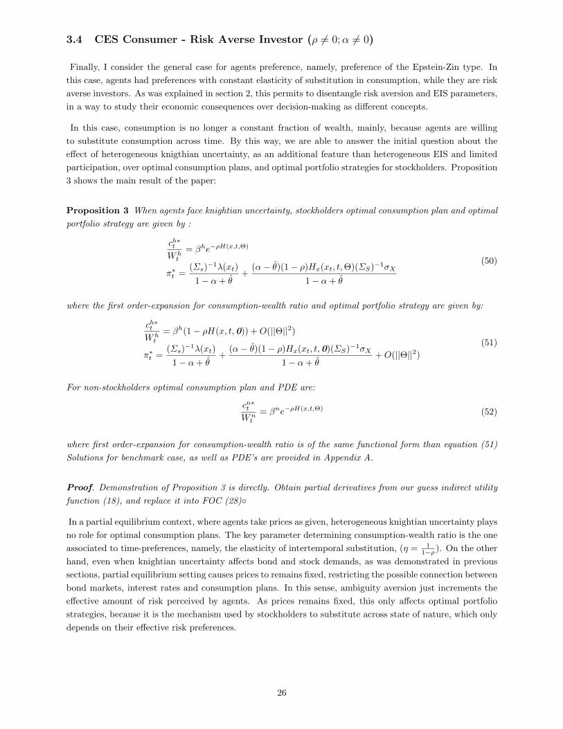
3.4 CES Consumer - Risk Averse Investor (ρ 6= 0;α 6= 0)

Finally, I consider the general case for agents preference, namely, preference of the Epstein-Zin type. In

this case, agents had preferences with constant elasticity of substitution in consumption, while they are risk

averse investors. As was explained in section 2, this permits to disentangle risk aversion and EIS parameters,

in a way to study their economic consequences over decision-making as different concepts.

In this case, consumption is no longer a constant fraction of wealth, mainly, because agents are willing

to substitute consumption across time. By this way, we are able to answer the initial question about the

effect of heterogeneous knigthian uncertainty, as an additional feature than heterogeneous EIS and limited

participation, over optimal consumption plans, and optimal portfolio strategies for stockholders. Proposition

3 shows the main result of the paper:

Proposition 3 When agents face knightian uncertainty, stockholders optimal consumption plan and optimal

portfolio strategy are given by :

ch∗tWht

= βhe−ρH(x,t,Θ)

π∗t =(Σs)

−1λ(xt)

1− α+ θ+

(α− θ)(1− ρ)Hx(xt, t,Θ)(ΣS)−1σX

1− α+ θ

(50)

where the first order-expansion for consumption-wealth ratio and optimal portfolio strategy are given by:

ch∗tWht

= βh(1− ρH(x, t,0)) +O(||Θ||2)

π∗t =(Σs)

−1λ(xt)

1− α+ θ+

(α− θ)(1− ρ)Hx(xt, t,0)(ΣS)−1σX

1− α+ θ+O(||Θ||2)

(51)

For non-stockholders optimal consumption plan and PDE are:

cn∗tWnt

= βne−ρH(x,t,Θ) (52)

where first order-expansion for consumption-wealth ratio is of the same functional form than equation (51)

Solutions for benchmark case, as well as PDE’s are provided in Appendix A.

Proof. Demonstration of Proposition 3 is directly. Obtain partial derivatives from our guess indirect utility

function (18), and replace it into FOC (28)

In a partial equilibrium context, where agents take prices as given, heterogeneous knightian uncertainty plays

no role for optimal consumption plans. The key parameter determining consumption-wealth ratio is the one

associated to time-preferences, namely, the elasticity of intertemporal substitution, (η = 11−ρ ). On the other

hand, even when knightian uncertainty affects bond and stock demands, as was demonstrated in previous

sections, partial equilibrium setting causes prices to remains fixed, restricting the possible connection between

bond markets, interest rates and consumption plans. In this sense, ambiguity aversion just increments the

effective amount of risk perceived by agents. As prices remains fixed, this only affects optimal portfolio

strategies, because it is the mechanism used by stockholders to substitute across state of nature, which only

depends on their effective risk preferences.

26

Optimal portfolio strategies also depends on stockholder time preferences. In particular, if agents are

relatively less willing to substitute consumption across time (low values for η) they reduce bonds demands,

substituting it for an increase on their stock demands. The same logic applies for relatively high values for η.

In particular, agents change their optimal total hedging demand, reflecting the effect on preference for hedge

from an increased trade-off between time-substitution and time-income effect. Previous cases considers that

η = 1 meaning that income and substitution effects associated to time change on state variables, in these

case the interest rate, cancel out. In the following, I provide some numerical results for ex-post consumption

distribution for each agent, and ex-post optimal portfolio distribution.

Table VI to VIII provides numerical results for ex-post expected value and standard deviation of empirical

distribution for optimal portfolio strategy. As expected, for any two given values of risk and ambiguity

aversion, optimal portfolio increase when agents are relatively less willing to substitute consumption across

time. On the other hand, standard deviation of optimal portfolio strategies increase when agents are less

willing to substitute across time.

However, is important to consider that these results are given for empirically relevant cases of EIS, namely,

when η < 1, where time-substitution effect dominates income effect. As was discuss in the introduction,

there are two empirical observation for parameters from Epstein-Zin preferences. First, that stockholders

prefer a late resolution of uncertainty (i.e α > ρ); and secondly, the empirical fact that stockholders have

higher EIS than non-stockhodlers. When η = 0.52, then α > ρ for all values of α. However, when risk

and uncertainty coexist, preferences for earlier or late resolution of uncertainty must be considered with

respect to the effective amount of risk (θ+ α). This leaves on cases where agents prefers a late resolution of

uncertainty, but an earlier resolution of ambiguity, (α < ρ < θ), but (ρ < α + θ). This last case is consider

for each degree of ambiguity aversion, while fixing η = 0.9 and = 1.2.

Finally Table VIII provides numerical results for ex-post consumption distribution for each agent. When

both agents had the same EIS, consumption plan performance are very similar, with no significant difference

on their expected value or standard deviation. As was discussed by Guvenen (2006), when there is no

differences between agents time-preferences, the volatility ratio is closed to one. However, the empirical

relevant case is to consider stockholders with higher EIS, than non-stockholders. When EIS for stockholders

is around η = 0.9, expected value for consumption to wealth ratio is about 106% with a standard deviation

of almost 0.05, while non-stockholders with EIS around η = 0.52, consumption to wealth ratio is around

160%, with a standard deviation of 0.43. As expected, this results suggest that heterogeneity on EIS and

limited participation on stock market helps to describe some important difference on optimal behavior of

stockholders and non-stockholders. However, partial equilibrium setting is to restrictive to study the effect

of heterogeneous knightian uncertainty on consumption plans as was originally proposed. As was explained

in these paper, this is because heterogeneous knightian uncertainty increase effective perceived risk of agents,

which affect optimal portfolio strategies. To study the effect on consumption plans, it will be necessary to

allow that prices reflects the increase of effective risk, and specially its effect on interest rate.

4 Conclusion

This paper study the effects of heterogeneous knightian uncertainty in a two-agent continuous time model

as an additional feature than heterogeneous EIS and limited participation in stock market. In a partial

equilibrium setting I ask if a meaningful distinction between risk and uncertainty, in the sense of Knight

27

(1929), is a key preference parameter determining optimal consumption plans for stockholders and non-

stockholder.

As both agents face different investment opportunities sets, fear about model misspecification will make

both agents doubt about the true data generating process. Non-stockholders choose a consumption plan

that maximizes his current utility process selecting endogenously the probability distribution that generates

the lowest expected value of future continuation utility. By the same way, stockholders choose not only a

consumption plan but also an optimal portfolio strategy on equity holdings. Given that both agents are

endowed with a common approximate model, when selecting their probability distribution they must incur

in a change of probability measure. After a change of measure each agent considers the same set of path

generated by the approximate model (and the underlying probability space), but they endogenously change

the likelihood of them. As non-stockholders are only concerned about the stochastic process of the state

variable they will put more probabilities in worst-case scenarios of just the state variables.

The main result of this paper is that in a partial equilibrium settings are not enough to explain the

effect of knightian uncertainty on consumption plans. As was demonstrated, knightian uncertainty increase

the effective amount of total risk perceived by agents affecting those decision variables directed related

to risk aversion, namely, optimal portfolio strategies. For three different preference specifications I show

that an increase in ambiguity aversion reduce optimal portfolio allocation on risky asset. On the other

hand, consumption plans are determined by time-preferences parameters. For a general class of preferences

of the Epstein-Zin type, being able to disentangle risk aversion from EIS parameters allows to conclude

that knightian uncertainty is not a key parameter determining consumption plans, something that may

be concluded erroneously using CRRA preferences. However, is expected that in a general equilibrium

setting, knightian uncertainty reveals it’s effect on consumption, via a price effect. in particular, while

knightian uncertainty increase effective risk, agents increase their demand for saving, as a precautionary

motive, affecting interest rate in equilibrium. As interest rate is the price of consumption over time, I expect

that this generates the mechanism proposed for knightian uncertainty as a extra motive for consumption

smoothing.

Also, this paper attempts to contribute to the increasing literature about ambiguity and knightian uncer-

tainty, and the behavioral understanding on decision makers facing risk and uncertainty as two different

motives. This paper shows the strong implications of robust decision-makers when they fear about model

misspecification.

28

5 Reference

1. Anderson E. W., L. P. Hansen, and T. J. Sargent (2003). A Quartet of Semigroups for Model Specifica-

tion, Robustness, Prices of Risk, and Model Detection. Journal of the European Economic Association,

Vol. 1, No. 1, pp. 68-123.

2. Basak S., and D. Cuoco (1998). An Equilibrium Model with Restricted Stock Market Participation.

The Review of Financial Studies 11.

3. Benigno P., and S. Nistico (2009). International Portfolio Allocation under Model Uncertainty. NBER

Working Paper Series.

4. Caballero R. and A. Krishnamurthy (2008). Collective Risk Management in a Flight to Quality

Episode. The Journal of Finance, VOL. LXIII, NO. 5, pp. 2195-2230

5. Camerer C., and M. Weber (1992). Recent Developments in Modeling Preferences: Uncertainty and

Ambiguity. Journal of Risk and Uncertainty, 5, pp. 325-370

6. Campbell, J. Y. (2003). Consumption-Based Asset Pricing. Handbook of the Economics of Finance,

Edited by G.M. Constantinides, M. Harris and R. Stulz Chap. 13, pp. 801-885.

7. Chen Z. and L. Epstein (2002). Ambiguity, Risk, and Asset Returns in Continuous Time. Economet-

rica, Vol. 70, No. 4, pp. 1403-1443.

8. Duffie, D., and L. Epstein (1992). Stochastic Differential Utility. Econometrica, Vol. 60, Issue 2, pp.

353-394

9. Duffie, D., and L. Epstein (1992). Asset Pricing with Stochastic Differential Utility. The review of

Financial Studies, Vol. 5, No. 3, pp. 411-436

10. Ellsberg, D. (1961). Risk, Ambiguity and the Savage Axioms. Quarterly Journal of Economics 75,

pp.643-669.

11. Epstein L. and M. Schneider (2003). Recursive multiple-priors. Journal of Economic Theory, 113, pp.

1-31.

12. Epstein L. and T. Wang (1994). Intertemporal Asset Pricing under Knightian Uncertainty. Econo-

metrica, Vol. 62, No. 3, pp.283-322.

13. Epstein L. and S. E. Zin (1989). Substitution, Risk Aversion, and the Temporal Behavior of Consump-

tion and Asset Returns: A Theoretical Framework. Econometrica, Vol. 57, No. 4, pp. 937-969.

14. Epstein L. and S. E. Zin (1991). Substitution, Risk Aversion, and the Temporal Behavior of Consump-

tion and Asset Returns: An Empirical Analysis. The Journal of Political Economy, Vol. 99, No. 2,

pp. 263-286

15. Fleming W.H., and H.M. Soner (1993). Controlled Markov processes and viscosity solutions. Applica-

tions of Mathematics, Springer, NewYork.

16. Gilboa I., and D. Schmeidler (1989). Maxmin Expected Utility with Non-Unique Prior, Journal of

Mathematical Economics 18, pp. 141-153.

29

17. Gomes F. and A. Michaelides (2008). Asset Pricing with Limited Risk Sharing and Heterogeneous

Agents. The Review of Financial Studies, vol. 21 No. 1, pp. 415-448.

18. Guvenen F. (2006). Reconciling conflicting evidence on the elasticity of intertemporal substitution: A

macroeconomic perspective. Journal of Monetary Economics. 53

19. Guvenen F. (2009): A parsimonious macroeconomic model for asset pricing, Econometrica, Vol.77, No.

6, 1711-1750.

20. Hall R. (1988). Intertemporal Substitution in Consumption. The Journal of Political Economy, Vol.

96, No. 2, pp. 339-357

21. Hansen L. P. and T. J. Sargent (2011). Wanting Robustness in Macroeconomics. In Benjamin M.

Friedman, and Michael Woodford, editors: Handbook of Monetary Economics, Vol. 3B, North-Holland,

pp. 1097-1157

22. Hansen L. P., T. J. Sargent, G. Turmuhambetova, and N. Williams (2006). Robust control and model

misspecification. Journal of Economic Theory, 128, pp. 45-90.

23. Hansen, L. P., and K. J. Singleton (1983). Stochastic Consumption, Risk Aversion, and the Temporal

Behavior of Asset Returns.” J.P.E 91: 249-265.

24. Karantounias A.G., L.P. Hansen, and T.J. Sargent (2009). Managing Expectations and Fiscal Policy.

Federal Reserve Bank of Atlanta. Working Paper Series.

25. Knight, F. H. (1921). Risk, Uncertainty and Profit. Houghton Mifflin Company.

26. Kraft H., F. T. Seifried, and M. Steffensen (2011). Consumption-Portfolio Optimization with Recursive

Utility in Incomplete Markets. Working Paper Series.

27. Lucas, R. E. (1978). Asset Prices in an Exchange Economy. Econometrica, 46. pp. 1426-1445.

28. Maenhout P.J. (2004). Robust portfolio Rules and Asset Pricing. The Review of Financial Studies,

vol. 17, N0. 4, pp. 951-983.

29. Malloy, C., T. Moskowitz, and A. Vissing-Jørgensen (2006). Long-Run Stockholder Consumption Risk

and Asset Returns. Working Paper, London Business School.

30. Mankiw N. G. and Zeldes S. P. (1991). The consumption of stockholders and nonstockholders. Journal

of Financial Economics, 29, pp. 97-112.

31. Mehra R., and E. Prescott (1985). The Equity Premium: A Puzzle. Journal of Monetary Economics

15, 145-161. North-Holland.

32. Onatski A., and J.H. Stock (2002). Robust Monetary Policy Under Model Uncertainty in a Small

Model of the U.S. Economy. Macroeconomic Dynamics, 6, pp. 85-110.

33. Orlik A. and I. Presno (2009). On Credible Monetary Policies with Model Uncertainty. Unpublished

paper, New York University.

34. Poterba J., Andrew A. Samwick, A. Shleifer, R. J. Shiller (1995). Stock Ownership Patterns, Stock

Market Fluctuations, and Consumption. Brookings Papers on Economic Activity, Vol. 1995, No. 2,

pp. 295-372.

30

35. Savage, L.J. (1954): The foundations of statistics. Wiley, NewYork.

36. Saito, M. (1995). Limited Market Participation and Asset Pricing.Working Paper, University of British

Columbia.

37. Vissing-Jørgensen A. (2002). Limited Asset Market Participation and the Elasticity of Intertemporal

Substitution. Journal of Political Economy, vol. 110, no. 4, pp. 825-853.

38. Woodford M. (2009). Robustly Optimal Monetary Policy with Near-Rational Expectations. NBER

Working Paper Series.

31

A Appendix: Propositions and Results

A.1 Existence and Uniqueness of SDU process of the Epstein-Zin Type

It is well know that the Epstein-Zin aggregator is non-Lipschitz, in the sense that there is no such constant

k > 0 that, for all c ∈ C and all (v, w) ∈ R we have |f(c, v) − f(c, w)| ≤ k|v − w|. As Duffie and Epstein

(1992, pp. 365-366) showed, that f is Lipschitz in utility and satisfies a growth condition in consumption are

typical for the existence and uniqueness of an associated stochastic differential utility index. Then, Theorem

1 and the principal results of Duffie and Epstein (1992), specially Proposition 9 about Bellman’s equation

for the optimal control problem, does not apply for aggregators of the Epstein-Zin type.

For existence of such utility process we have to recall on a weaker condition than Lipschitz, saying, that for

some k > 0 and v ≥ w we have:

f(c, v)− f(c, w) ≤ k(v − w)

Using the previous property, Kraft, Seifried and Steffensen (2011) showed that by the homotheticity property

of (13), existence and uniqueness can be established at least in purely Brownian setting (see also Schroder and

Skiadas (1999)). They also provide a Verification Theorem, more general than the one propused by Duffie

and Epstein (1992) for a canonical stochastic optimal control problem with recursive preference (Kraft,

Seifried and Steffensen (2011). Theorem 3.1, pp. 7). Here, and following standard practice, I will take

existence and uniqueness of stochastic differential utility indices for granted.

The previous setting leave us on two cases:

1. k = −βαρ > 0 and α < 0 < ρ

2. k = −βαρ > 0 and ρ < 0 < α

A.2 A Multiplier or Penalty Robust Control Problems.

In this paper, I will consider the robust control theory approach of Hansen, Sargent, Turmuhambetova,

Williams (2006), in which agents choose robust policy functions in the sense that they are invariant to model

misspecification. In particular, I will adopt the martingale approach, which are games on fixed probability

spaces.

In the following, it will be necessary to define a preference for robustness, then, define the set of priors,

which captures the idea that models are approximations to each other, and finally, define the robust control

problem for each agent. However, in an intermediate step we transform the canonical set of priors to

a dynamic representation of non-negative martingales and likelihood ratios, which allows to work on the

original probability space and with non-negative martingales, instead of working with multiple distributions

and probability spaces. In this context a definition of the finite interval absolute continuity property will be

necessary.

Preference.

First, it is necessary to construct a preference for robustness. Following Hansen et al. (2006), and as

32

in the previous section, consider that the n-dimensional Brownian motion induces a multivariate Wiener

measure P 0 on a canonical space (Ω∗,F∗) defined as follow. Let Ω∗ be the space of continuos functions

f : [0,+∞) → Rn. Let F∗ be the Borel sigma algebra for the restriction of the continuous functions f to

[0, t], where open sets are defined using the sup-norm over this interval. Let F∗ be the smallest sigma algebra

containing F∗t for t ≥ 0. An event in F∗t restricts the properties of the continuous functions only on the finite

interval [0, t]. For any probability measure P on (Ω∗,F∗), let Pt denote the restriction to F∗t . In particular,

the Brownian motion B induces a multivariate Wiener measure on (Ω∗,F∗), which we denote P 0

The set of Priors.

In a way to make explicit the idea that models are approximations to each others, and that agents can

not distinguish it with finite data sets, we are interested in probability distributions that are absolutely

continuous with respect to Wiener measures. Roughly speaking, as was pointed by Hansen et. al. (2006)

absolute continuity over finite intervals (a weaker condition than absolutely continuity) requires that when

comparing two measures both assigned positive probability in the same events, except on tail events. Let

P be the set of all distributions that are absolutely continuous with respect to P 0 over finite intervals. We

now turn to the question of how to construct P.

To limit the alternative models that the decision-maker entertains, we now construct a relative entropy mea-

sure for a perturbed stochastic process. Relative entropy measures the discrepancy between the probability

distribution P 0 and any P ∈ P, defined as the expected value of the log-likelihood between Pt and P 0t :

R∗(P ) =

(∫log

(dPtdP 0

t

)dPt

)(53)

where dPtdP 0t

is the Radon-Nikodym derivative of Pt with respect to P 0t . Hansen et al. (2006) show that

requiring that entropy be finite restricts the form that model misspecification can take. Finiteness of entropy

implies that admissible perturbations of the approximating model must be absolutely continuous with respect

to it over finite intervals.

Hansen et al. (2006) show that requiring that entropy be finite restricts the form that model misspecification

can take. Finiteness of entropy implies that admissible perturbations of the approximating model must be

absolutely continuous with respect to it over finite intervals.

To formulate the recursive version of the multiplier probability games presented in Hansen et al. (2006,

Definition 5.2 pp. 58) it is convenient to represent alternative model specifications as martingale “preference

shocks” on a common probability space. This allows to work on the original (Ω,F, P 0) and with nonnegatives

martingales, instead on (Ω∗,F∗) and multiple distributions. In other words, define an auxilary random

variable on the original probability space that permit us change measures from one probability distribution

to another, but with the property that the same original set of sequence would be consider. Then, for

diffusion process, a change of measure change the mean rate or drift of the process, but not it’s volatility.

As was explain, after a change of measure the agent puts more probability on those sequences that are more

distant from the original mean sequence.

Define zt = dPtdP 0t

on (Ω,F, P 0). zt is a nonnegative martingale adapted to the filtration Ft : t ≥ 0 with

Ezt = 1. Moreover, ∫ftdPt = E(ztft(B)) (54)

33

(for any bounded and F∗t ) measurable function ft (For a technical proof see Shreve (2004) pp. 210-212). By

the Martingale Representation Theorem, any martingale z with unit expectation can be described by:

zt = 1 +

∫ t

0

zuhudBu (55)

and z solves the differential equation,

dzt = zthtdBt with initial condition z0 = 1 (56)

For the representation of non-sequential penalty problem, Hansen et al. (2006, Definition 5.2) introduces a

new state variable zt, initialized at one, and take ht to be under control of the minimizing agent.

By this way, we are now able to represent likelihood ratios as function of a nonnegative martingale z and a

progressively measurable function h. It is well know that a solution to the difference equation (56), is of the

form,

zt = exp

(∫ t

0

hudBu −1

2

∫ t

0

|hu|2du)

(57)

lt =

(∫ t

0

hudBu −1

2

∫ t

0

|hu|2du)

(58)

which is exactly a likelihood ratio (and log-likelihood ratio, respectively) of two measures under the Brownian

motion B. A very important result in modern financial models is the Girsanov Theorem, that implies:

If for all t ≥ 0, Pt is absolutely continuous with respect to P 0t , then P is the induced distribution for a

solution B to a stochastic differential equation defined on a probability space (Ω,F, P ):

dBt = htdt+ dBt (59)

for some progressively measurable h defined on (Ω∗,F∗) and some Brownian motion B that is adapted to

Ft : t ≥ 0. Moreover, for each t,

P

(∫ t

0

|hu|2du <∞)

= 1 (60)

(for a proof see Shreve (2004), pp.212).

Now we are able to define a discounted entropy measure for nonnegative martingales:

R∗(z) =1

2E

(∫ ∞0

zt|ht|2dt)

(61)

A.3 Comparison of Results from Benchmark Case and Penalty Robust Control

Problems and explicit PDE’s

In this section, I present explicit form solutions for benchmark and penalty robust control cases, as well

as explicit form for PDE’s. In the following, proposition 3 present results when both agents are log-utility

consumer-investors (ρ = α = 0).

34

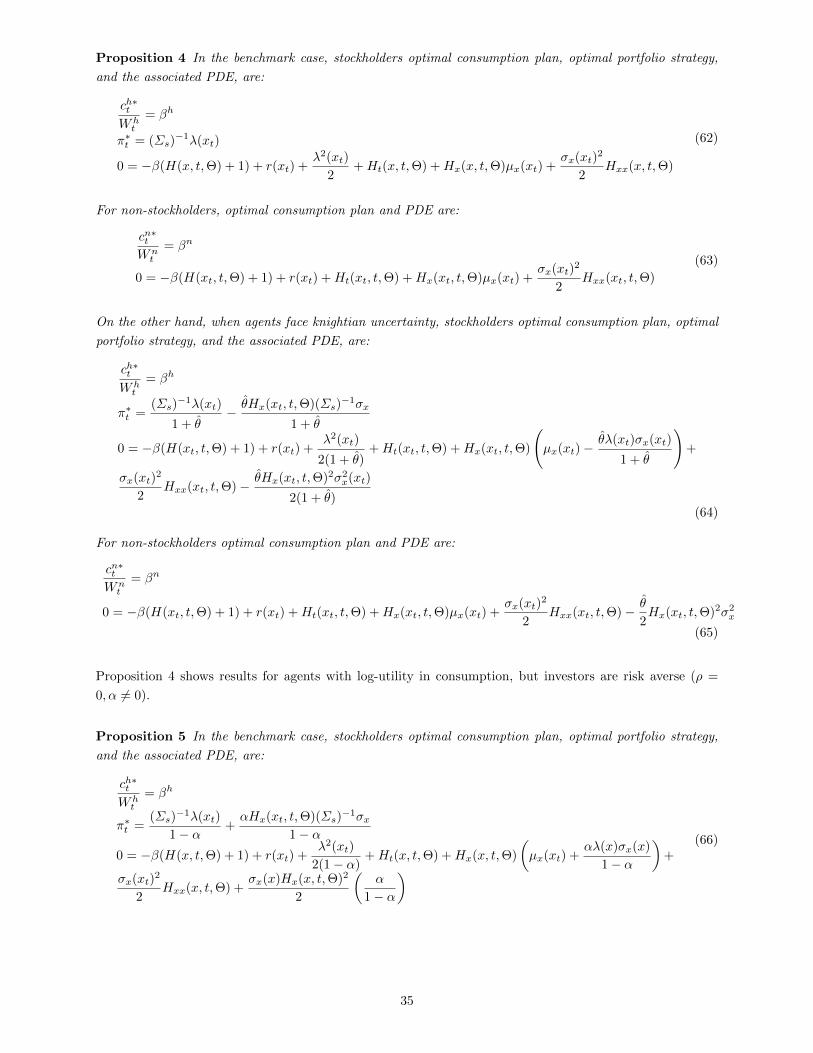
Proposition 4 In the benchmark case, stockholders optimal consumption plan, optimal portfolio strategy,

and the associated PDE, are:

ch∗tWht

= βh

π∗t = (Σs)−1λ(xt)

0 = −β(H(x, t,Θ) + 1) + r(xt) +λ2(xt)

2+Ht(x, t,Θ) +Hx(x, t,Θ)µx(xt) +

σx(xt)2

2Hxx(x, t,Θ)

(62)

For non-stockholders, optimal consumption plan and PDE are:

cn∗tWnt

= βn

0 = −β(H(xt, t,Θ) + 1) + r(xt) +Ht(xt, t,Θ) +Hx(xt, t,Θ)µx(xt) +σx(xt)

2

2Hxx(xt, t,Θ)

(63)

On the other hand, when agents face knightian uncertainty, stockholders optimal consumption plan, optimal

portfolio strategy, and the associated PDE, are:

ch∗tWht

= βh

π∗t =(Σs)

−1λ(xt)

1 + θ− θHx(xt, t,Θ)(Σs)

−1σx

1 + θ

0 = −β(H(xt, t,Θ) + 1) + r(xt) +λ2(xt)

2(1 + θ)+Ht(xt, t,Θ) +Hx(xt, t,Θ)

(µx(xt)−

θλ(xt)σx(xt)

1 + θ

)+

σx(xt)2

2Hxx(xt, t,Θ)− θHx(xt, t,Θ)2σ2

x(xt)

2(1 + θ)(64)

For non-stockholders optimal consumption plan and PDE are:

cn∗tWnt

= βn

0 = −β(H(xt, t,Θ) + 1) + r(xt) +Ht(xt, t,Θ) +Hx(xt, t,Θ)µx(xt) +σx(xt)

2

2Hxx(xt, t,Θ)− θ

2Hx(xt, t,Θ)2σ2

x

(65)

Proposition 4 shows results for agents with log-utility in consumption, but investors are risk averse (ρ =

0, α 6= 0).

Proposition 5 In the benchmark case, stockholders optimal consumption plan, optimal portfolio strategy,

and the associated PDE, are:

ch∗tWht

= βh

π∗t =(Σs)

−1λ(xt)

1− α+αHx(xt, t,Θ)(Σs)

−1σx1− α

0 = −β(H(x, t,Θ) + 1) + r(xt) +λ2(xt)

2(1− α)+Ht(x, t,Θ) +Hx(x, t,Θ)

(µx(xt) +

αλ(x)σx(x)

1− α

)+

σx(xt)2

2Hxx(x, t,Θ) +

σx(x)Hx(x, t,Θ)2

2

(α

1− α

)(66)

35

For non-stockholders, optimal consumption plan and PDE are:

cn∗tWnt

= βn

0 = −β(H(xt, t,Θ) + 1) + r(xt) +Ht(xt, t,Θ) +Hx(xt, t,Θ)µx(xt) +σx(xt)

2

2Hxx(xt, t,Θ)

+ασx(xt)

2Hx(xt, t,Θ)2

2

(67)

On the other hand, when agents face knightian uncertainty, stockholders optimal consumption plan, optimal

portfolio strategy, and the associated PDE, are:

ch∗tWht

= βh

π∗t =(ΣS)−1λ(xt)

1− α+ θ+

(α− θ)Hx(xt, t,Θ)(ΣS)−1σX

1− α+ θ

0 = −β(H(xt, t,Θ) + 1) + r(xt) +λ2(xt)

2(1− α+ θ)+Ht(xt, t,Θ) +Hx(xt, t,Θ)

(µx(xt) +

(α− θ)λ(xt)σx(xt)

1− α+ θ

)+σx(xt)

2

2Hxx(xt, t,Θ) +

(α− θ)Hx(xt, t,Θ)2σ2x(xt)

2(1− α+ θ)(68)

For non-stockholders optimal consumption plan and PDE are:

cn∗tWnt

= βn

0 = −β(H(xt, t,Θ) + 1) + r(xt) +Ht(xt, t,Θ) +Hx(xt, t,Θ)µx(xt) +σx(xt)

2

2Hxx(xt, t,Θ)

+(α− θ)

2Hx(xt, t,Θ)2σ2

x

(69)

Finally, Proposition 5 shows results for agents with log-utility in consumption, but investors are risk averse

(ρ 6= 0, α 6= 0).

Proposition 6 In the benchmark case, stockholders optimal (log-) consumption/wealth plan, optimal port-

folio strategy, and the associated PDE, are:

Ch∗t = log βh − ρH(x, t,Θ)

π∗t =(Σs)

−1λ(xt)

1− α+α(1− ρ)Hx(xt, t,Θ)(Σs)

−1σx1− α

0 =β

ρ

((1− ρ)e−ρH(x,t,Θ) − 1

)+ r(xt) +

λ2(xt)

2(1− α)+ (1− ρ)Ht(x, t,Θ) + (1− ρ)Hx(x, t,Θ)

(µx(xt) +

αλ(x)σx(x)

1− α

)+

σx(xt)2

2(1− ρ)Hxx(x, t,Θ) +

σx(x)(1− ρ)Hx(x, t,Θ)2

2

(α

1− α

)(70)

For non-stockholders, optimal consumption plan and PDE are:

Cn∗t = log βn − ρH(x, t,Θ)

0 =β

ρ

((1− ρ)e−ρH(x,t,Θ) − 1

)+ r(xt) + (1− ρ)Ht(x, t,Θ) + (1− ρ)Hx(x, t,Θ)µx(xt)+

σx(xt)2

2(1− ρ)Hxx(x, t,Θ) +

σx(x)(1− ρ)Hx(x, t,Θ)2α

2

(71)

36

On the other hand, when agents face knightian uncertainty, stockholders optimal consumption plan, optimal

portfolio strategy, and the associated PDE, are:

Ch∗t = log βh − ρH(x, t,Θ)

π∗t =(Σs)

−1λ(xt)

1− α+ θ+

(α− θ)(1− ρ)Hx(xt, t,Θ)(ΣS)−1σX

1− α+ θ

0 =β

ρ

((1− ρ)e−ρH(x,t,Θ) − 1

)+ r(xt) +

λ2(xt)

2(1− α+ θ)+ (1− ρ)Ht(xt, t,Θ) +

σx(xt)2

2(1− ρ)Hxx(xt, t,Θ)

+Hx(xt, t,Θ)(1− ρ)

(µx(xt) +

(α− θ)λ(xt)σx(xt)

1− α+ θ

)+

(α− θ)((1− ρ)Hx(xt, t,Θ)σx(xt))2

2(1− α+ θ)

(72)

For non-stockholders optimal consumption plan and PDE are:

Cn∗t = log βn − ρH(x, t,Θ)

0 =β

ρ

((1− ρ)e−ρH(x,t,Θ) − 1

)+ r(xt) + (1− ρ)Ht(xt, t,Θ) + (1− ρ)Hx(xt, t,Θ)µx(xt) +

σx(xt)2

2(1− ρ)Hxx(xt, t,Θ)

+(α− θ)

2((1− ρ)Hx(xt, t,Θ)σx(xt))

2

(73)

B Knigthian Uncertainty, Preference for Robustness and Learn-

ing

At this point it is important to ask which is actually the amount of ambiguity or knightian uncertainty

on financial markets? Consider some interesting examples of financial and macroeconomics models that use

ambiguity to explain some well-known puzzles.

For example, Epstein and Schneider (2010) provide a large review of literature considering ambiguous

situations and taking ambiguity aversion seriously to explain the following financial anomalies: Equity

premium and risk free rate puzzles, were studied by Chen and Epstein (2002), Anderson, Hansen and

Sargent (2003), and Maenhout (2004), in models of consumption-based asset pricing, where both, risk and

uncertainty were priced in equilibrium. Another examples are the home-bias puzzle and flight to quality

portfolio effects, each of them were studied recently by Benigno and Nistico (2009), and Caballero and

Krishnamurthy (2008), respectively.

Moreover, macroeconomic literature has been studying optimal and time-consistent fiscal and monetary

policy with model misspecification. Onatski and Stock (2002), Orlik and Presno (2009) and Woodford

(2009), provide answers on monetary policy, while Karantounias et al. (2009) studied optimal fiscal policy,

where typically a representative household uses a set of alternative probability models on the exogenous

state of the economy. In such settings, households’ expectations becomes a powerful channel for both fiscal

and monetary policymaking to achieve their respectively objectives.

Chen and Epstein (2002) present a general framework on dynamic context for modeling choice situations

featuring “Knightian Uncertainty” or “Ambiguity”. In that work, a recursive multiple-priors utility model

was introduce, which is an extension of stochastic differential utility (SDU) of Duffie and Epstein (1992).

The former author replaced the usual single prior setting by a set of priors, as in the atemporal model of

37

Gilboa and Schmeidler (1989), which satisfies regularity conditions and also a property that they called

rectangularity.

On the other hand, Hansen, et al. (2006) link the max-min expected utility theory of Gilboa and Schmeidler

(1989) to applications of stochastic robust control theory of James (1992), Petersen, James and Dupuis

(2002). In that work, they present two ways, a non-sequential and a recursive formulation, for different two-

player zero-sum games that yield robust decision rules. Hansen et. al. (2006) consider a decision maker who

fears that data are generated by a restricted statistical perturbation of an approximated model, restricted

by the degree of uncertainty aversion of the agent (i.e. the rate of substitution between the approximated

model and the maximum statistical perturbation tolerated by the agent).

Even that the previous question is an empirical one, I want to motivate it in two directions: Agents

preference for Robustness on atemporal setting; and data, information, and learning on multiperiod settings.

It is important to be clear that in this paper I’m not going to deal with the question about learning with

ambiguity markets, it is just presented as a motivation for being one of the most important critics to knightian

uncertainty.

B.1 Agents Preference for Robustness on Atemporal Settings

Kinght’s (1921) distinction between risk and uncertainty could be described as follow: A random variable

is risky if its probability distribution is known, uncertain if its distribution is unknown. In his book “Risk,

Uncertainty and Profit”, he argued that uncertainty in is much more common in economic environment than

risky situations. However, as decision theory evolves, Bayesian approach (i.e. the existence of any prior

underlying choices) seems like captures the fundamentals on decision-making. Under the Bayesian approach,

Knight’s distinction has no interesting consequences. In Bayesian theory, decision makers act so as to

maximize the expected value of their gain, no matter whether the fluctuations faced are risky or uncertain.

Moreover, Savage (1954) constructed an axiomatic treatment of decision-making in which preferences over

gambles could be represented by maximizing expected utility under subjective probabilities, extending earlier

works of von Neumann and Morgenstern (1944), which assumed objective probabilities for expected utility

gambles

Knight’s idea was not only an intuitive inspection of economic environments, but appears to have significant

effect on economic agents behavior. The most notably example relates to Ellsberg (1961) urn’s experiments,

where he shows that agents are really uncertainty averse, meaning that they reflect a preference for knowing

probabilities over having to form them subjectively (see more about experimental and market based evidence

on Camerer and Weber (1992)). Evidently, this contradicts the Bayesian paradigm, and particularly Savage

axiomatization of decision making. Moreover, rational expectation theory withdrew freedom from Savage’s

decision theory by imposing equality between agent’s subjective probabilities and the true data generating

process. As Hansen and Sargent (2010) emphasized, because rational expectation abandons Savage’s personal

theory of probability, it can be argued that rational expectations indirectly increase the appeal of Knight’s

distinction between risk and uncertainty.

There are mainly two ways of how decision theory extend Bayesian models and Savage axioms. The first of

them is due to Bewley (1986), who basically drops the completeness axiom from the extension of Savage’s

theory made by Anscombe and Aumann (1963), and add an assumption of inertia.17

17In Bewley’s words: “The completeness assumption asserts that any two lotteries are comparable in the preference order-

38

On the other hand, Gilboa and Schmeidler (1989) provide a weaker set of axioms that included a notion

of uncertainty aversion. In particular, what Gilboa and Schmeidler (1989) provided was a weaker version of

Savage’s Sure-Thing Principle, which consequently replace preference representation and beliefs of a single

prior by a set of priors, and a decision-maker who uses worst case scenarios among this family to evaluate

unknown outcomes.

B.2 Data, Information, and Learning on Multiperiod Settings

The previous discussion was motivated in atemporal games and deals with one-shot choices from decision-

makers. However, most financial and macroeconomic problems arise in dynamic setting with multiple choices

over time. This renders to refocus our discussion of knightian uncertainty in intertemporal settings. For this,

it will be interesting to center our attention on three interrelated concepts: data, information, and learning.

Since the last 20 decades a lot of efforts had been done to construct axiomatized and non-axiomatized

extensions (on discrete and continuous time) of Gilboa and Schmeidler (1989) atemporal multiple-priors

model. One class of them centers on the construction of recursive multiple-priors utility models, where

non-axiomatized examples are Epstein and Wang (1994) on discrete time, and Chen and Epstein (2002) on

continuous time; alternatively, Epstein and Schneider (2003), provide an axiomatized version of multiple

priors utility. Another class of models that captures knightian uncertainty relies on applications of robust

decision-making and are associated to two-player zero-sum games of Fleming and Soner (2006), as for ex-

ample, Anderson, Hansen, Sargent (2003), and Hansen, Sargent, Turmuhambetova, and Williams (2006).

Three important topics arise from these classes of models: observational equivalence, dynamic consistency

and learning.

Observational equivalence happens when we observed realized outcomes that are consistent with two different

theories. In the present setting, one important question is how we can detect that agents choose endogenously

a given probability distribution, and it was not the distribution that the agent was endowed at the first time?

Despite that related literature relies on argumental justification for this problem, in my opinion there is only

one way to avoid this problem: data. When talking about ambiguity scenarios, we are considering both, that

agents can not statistically distinguish two probability models with an available finite set of information, and

that agents fear about model misspecification. This mean that the decision maker seeks robustness against

models that can be distinguished from the approximated model with an infinite data set (there is a Law of

Large Number that applies under the approximated model, but delivers a different limit under alternative

models, or may not converge); but because of finite log-likelihood ratios, they are impossible to distinguish

from a finite data set. This suggest that ambiguity scenarios may not last infinitely, and they should occur

over finite time length, and probably on very short ones.

On the other hand, dynamic consistency is a key element to obtain recursivity in utility. When dealing with

ambiguity, the construction of the set of priors will determine the ability to construct a dynamic version

of the atemporal problem of Gilboa and Schmeidler (1989). While Chen and Epstein (2002) relies on a

ing;(...) When this axiom is dropped, one obtains a set of subjective probability distributions rather than a single one. One

lottery is preferred to another if its expected value is higher according to all the distributions. The idea of the inertia assump-

tion is that a person never accepts a lottery unless he prefers acceptance to rejection. There is a status quo with which he

stays unless an alternative is preferred. Without the inertia assumption, choices between all incomparable alternatives would

be arbitrary. I apply the adjective “Knightian” to behavior consistent with the assumptions just described.”

39

strict restriction on the set of priors, called rectangularity18 to obtain recursivity on utility, the Robust

control approach generates the set of priors by a given level of tolerance associated to the relative entropy

index, which measures distance between probability distributions. Both consider ways to attain dynamic

consistency in each settings.19

A more attractive question has to do with updating and learning in ambiguous settings. As Chen and Epstein

actually exposed, “would ambiguity not disappear eventually as the agents learns about her environment?.”

Learning is typically used to criticize models of ambiguity, since ambiguity is due to a lack of information

and, it could be resolved as agents learn. However, this is consistent with our previous discussion about the

reasons of why ambiguity might be probably a short run phenomenon. Another approach of learning, has

to do with it’s effects on the construction of probability sets over time. A formal treatment of models under

ambiguity has not been developed until Epstein and Schneider (2005), which provides a generalization of

the Bayesian learning model that can accommodate the distinction between risk and uncertainty. Under

recursive multiple-priors utility, learning is completely determined by a set of probability measures, and

measure-by-measure bayesian updating described response to data.

18For more on rectangularity, see the axiomatized version of Epstein and Scheneider (2003).19For discussion relating both approaches, see Hansen, Sargent, Turmuhambetova, and Williams (2006).

40

Table 1: U.S. Quarterly data 1947.II - 1996.IV

Panel A: Statistics

if rf µS µS − rf

Mean .012 .0022 .019 .0071

Standard Deviation .0074 .0063 .076 .077

Panel B: Parameters

κ 1.25101 βs = βn 0.06

r 0.0024

σs 0.0763

Φ 1.88

φ 0.0127

Source: Campbell(1999)

Table 2: Simulation results for empirical moments of π when ρ = α = 0 (η = γ = 1)

r = 0.24% ¯r = 0.2% ¯r = 0.3%

θ E(π) σ(π) θ E(π) σ(π) θ E(π) σ(π)

0 1.213 0.04953 0 1.101 0.0482 0 1.356 0.051

0.1 1.104 0.04513 0.1 1.0025 0.04392 0.1 1.2346 0.0464

0.2 1.014 0.04149 0.2 0.92 0.04037 0.2 1.133 0.0426

0.3 0.937 0.03843 0.3 0.851 0.03738 0.3 1.048 0.0394

0.4 0.8717 0.03583 0.4 0.7913 0.03484 0.4 0.9745 0.0367

0.5 0.8148 0.03359 0.5 0.7397 0.03266 0.5 0.911 0.0344

41

Table 3: Simulation results for empirical moments of ex-post indirect utility when ρ = α = 0 (η = γ = 1)

r = 0.24% ¯r = 0.2% ¯r = 0.3%

AA rules RE rules AA rules RE rules AA rules RE rules

θ E(J∗) σ(J∗) E(J) σ(J) θ E(J∗) σ(J∗) E(J) σ(J) θ E(J∗) σ(J∗) E(J) σ(J)

0 -2.81427 0.0459 -2.81427 0.0459 0 -2.81377 0.04416 -2.81377 0.04416 0 -2.81495 0.04834 -2.81495 0.04834

0.1 -2.81427 0.04373 -2.81444 0.0461 0.1 -2.81378 0.04233 -2.81393 0.04434 0.1 -2.81493 0.04575 -2.81513 0.0486

0.2 -2.81416 0.04204 -2.81454 0.0463 0.2 -2.8137 0.0409 -2.81404 0.0445 0.2 -2.81478 0.0437 -2.81523 0.04883

0.3 -2.814 0.0407 -2.8146 0.04648 0.3 -2.81358 0.0398 -2.81411 0.04464 0.3 -2.81456 0.0421 -2.81526 0.049

0.4 -2.81381 0.03964 -2.81462 0.04664 0.4 -2.81344 0.0389 -2.81414 0.04478 0.4 -2.81429 0.04075 -2.81525 0.04925

0.5 -2.8136 0.0388 -2.8146 0.0468 0.5 -2.81329 0.0382 -2.81415 0.0449 0.5 -2.81401 0.03971 -2.8152 0.0494

Table 4: Simulation results for empirical moments of π, πmyopic,πhedge when ρ = 0 and α 6= 0 (η = 1; γ 6= 1)

Panel A: E(π)

θ | γ 1.2 1.1 1 0.9 0.8 0.7

0 1.01499 1.10556 1.21425 1.3471 1.51315 1.72665

0.1 0.938344 1.01499 1.10556 1.21425 1.3471 1.51315

0.2 0.872652 0.938344 1.01499 1.10556 1.21425 1.3471

0.3 0.815719 0.872652 0.938344 1.01499 1.10556 1.21425

0.4 0.765902 0.815719 0.872652 0.938344 1.01499 1.10556

0.5 0.721947 0.765902 0.815719 0.872652 0.938344 1.01499

Panel B: E(πmyopic)

θ | γ 1.2 1.1 1 0.9 0.8 0.7

0 1.01188 1.10387 1.21425 1.34917 1.51781 1.73465

0.1 0.93404 1.01188 1.10387 1.21425 1.34917 1.51781

0.2 0.867323 0.93404 1.01188 1.10387 1.21425 1.34917

0.3 0.809501 0.867323 0.93404 1.01188 1.10387 1.21425

0.4 0.758907 0.809501 0.867323 0.93404 1.01188 1.10387

0.5 0.714266 0.758907 0.809501 0.867323 0.93404 1.01188

Panel C: E(πhedge)

θ | γ 1.2 1.1 1 0.9 0.8 0.7

0 0.00310894 0.00169579 0. -0.00207263 0.004694 -0.00799443

0.1 0.00430469 0.00310894 0.00169579 0. -0.00207263 -0.00466341

0.2 0.00532962 0.00430469 0.00310894 0.00169579 0. -0.00207263

0.3 0.00621789 0.00532962 0.00430469 0.00310894 0.00169579 0.

0.4 0.00699512 0.00621789 0.00532962 0.00430469 0.00310894 0.00169579

0.5 0.00768092 0.00699512 0.00621789 0.00532962 0.00430469 0.00310894

42

Table 5: Simulation results for empirical moments of π, πmyopic,πhedge when ρ = 0 and α 6= 0 (η = 1; γ 6= 1)

Panel A: σ(π)

θ | γ 1.2 1.1 1 0.9 0.8 0.7

0 0.0423637 0.0460783 0.0505654 0.0560828 0.0630169 0.0719752

0.1 0.0392432 0.0423637 0.0460783 0.0505654 0.0560828 0.0630169

0.2 0.0365894 0.0392432 0.0423637 0.0460783 0.0505654 0.0560828

0.3 0.0343087 0.0365894 0.0392432 0.0423637 0.0460783 0.0505654

0.4 0.032331 0.0343087 0.0365894 0.0392432 0.0423637 0.0460783

0.5 0.0306027 0.032331 0.0343087 0.0365894 0.0392432 0.0423637

Panel B: σ(πmyopic)

θ | γ 1.2 1.1 1 0.9 0.8 0.7

0 0.0421378 0.0459685 0.0505654 0.0561838 0.0632067 0.0722363

0.1 0.0388965 0.0421378 0.0459685 0.0505654 0.0561838 0.0632067

0.2 0.0361181 0.0388965 0.0421378 0.0459685 0.0505654 0.0561838

0.3 0.0337103 0.0361181 0.0388965 0.0421378 0.0459685 0.0505654

0.4 0.0316034 0.0337103 0.0361181 0.0388965 0.0421378 0.0459685

0.5 0.0297444 0.0316034 0.0337103 0.0361181 0.0388965 0.0421378

Panel C: σ(πhedge)

θ | γ 1.2 1.1 1 0.9 0.8 0.7

0 0.00226987 0.00123811 0. 0.00151325 0.00340481 0.00583682

0.1 0.0031429 0.00226987 0.00123811 0. 0.00151325 0.00340481

0.2 0.00389121 0.0031429 0.00226987 0.00123811 0. 0.00151325

0.3 0.00453975 0.00389121 0.0031429 0.00226987 0.00123811 0.

0.4 0.00510722 0.00453975 0.00389121 0.0031429 0.00226987 0.00123811

0.5 0.00560792 0.00510722 0.00453975 0.00389121 0.0031429 0.00226987

43

Table 6: Simulation results for empirical moments of E(π) when ρ 6= 0 and α 6= 0 (η 6= 1; γ 6= 1)

η = 0.52

θ | γ 1.2 1.1 1 0.9 0.8 0.7

0 1.01986 1.10772 1.21314 1.342 1.50306 1.71015

0.1 0.945523 1.01986 1.10772 1.21314 1.342 1.50306

0.2 0.881804 0.945523 1.01986 1.10772 1.21314 1.342

0.3 0.826581 0.881804 0.945523 1.01986 1.10772 1.21314

0.4 0.778261 0.826581 0.881804 0.945523 1.01986 1.10772

0.5 0.735625 0.778261 0.826581 0.881804 0.945523 1.01986

η = 0.9

θ | γ 1.2 1.1 1 0.9 0.8 0.7

0 1.01611 1.10567 1.21314 1.3445 1.50869 1.7198

0.1 0.940328 1.01611 1.10567 1.21314 1.3445 1.50869

0.2 0.875373 0.940328 1.01611 1.10567 1.21314 1.3445

0.3 0.819078 0.875373 0.940328 1.01611 1.10567 1.21314

0.4 0.76982 0.819078 0.875373 0.940328 1.01611 1.10567

0.5 0.726357 0.76982 0.819078 0.875373 0.940328 1.01611

Table 7: Simulation results for empirical moments of σ(π) when ρ 6= 0 and α 6= 0 (η 6= 1; γ 6= 1)

η = 0.52

θ | γ 1.2 1.1 1 0.9 0.8 0.7

0 0.0424467 0.0455597 0.049638 0.0550112 0.0621675 0.0718669

0.1 0.0400672 0.0424467 0.0455597 0.049638 0.0550112 0.0621675

0.2 0.0382531 0.0400672 0.0424467 0.0455597 0.049638 0.0550112

0.3 0.0368795 0.0382531 0.0400672 0.0424467 0.0455597 0.049638

0.4 0.035852 0.0368795 0.0382531 0.0400672 0.0424467 0.0455597

0.5 0.0350976 0.035852 0.0368795 0.0382531 0.0400672 0.0424467

η = 0.9

θ | γ 1.2 1.1 1 0.9 0.8 0.7

0 0.0418522 0.0453384 0.049638 0.0550234 0.0619026 0.0709158

0.1 0.0389904 0.0418522 0.0453384 0.049638 0.0550234 0.0619026

0.2 0.0366175 0.0389904 0.0418522 0.0453384 0.049638 0.0550234

0.3 0.034634 0.0366175 0.0389904 0.0418522 0.0453384 0.049638

0.4 0.0329649 0.034634 0.0366175 0.0389904 0.0418522 0.0453384

0.5 0.0315529 0.0329649 0.034634 0.0366175 0.0389904 0.0418522

44

Table 8: Simulation results for empirical moments of ck when ρ 6= α 6= 0 (η 6= γ 6= 1)

η = 0.52 E(ck) σ(ck)

Stokholders 1.62377 0.436298

Non-stockholders 1.62018 0.433825

η = 0.9 E(ck) σ(ck)

Stokholders 1.06042 0.0484775

Non-stockholders 1.06002 0.0482027

Figure 1: Behavior of Stock Demands and its components relative to the level of prices when ρ = α = 0

(η = γ = 1).

(a) Stock Demand (b) Myopic Demand

(c) Hedge Demand

45

Figure 2: Behavior of Stock Demand relative to the level of prices when ρ = 0 and α 6= 0 (η = 1 and γ 6= 1).

(a) Stock Demand when γ = 1.2 (b) Stock Demand when γ = 0.7

(c) Stock Demand for low level of r(x) (d) Stock Demand for low high of r(x)

46

Figure 3: Behavior of Myopic Demand relative to the level of prices when ρ = 0 and α 6= 0 (η = 1 and

γ 6= 1).

(a) Myopic Demand when γ = 1.2 (b) Myopic Demand when γ = 0.7

(c) Myopic Demand for low level of λ(x) (d) Myopic Demand for low high of λ(x)

47

Figure 4: Behavior of Hedge Demand relative to the level of prices when ρ = 0 and α 6= 0 (η = 1 and γ 6= 1).

(a) Hedge Demand when γ = 1.2 (b) Hedge Demand when γ = 0.6

(c) Hedge Demand for low level of r(x) (d) Hedge Demand for low high of r(x)

48