DOCUMENTO DE TRABAJO Instituto de Economía TESIS de MAGÍSTER INSTITUTO DE ECONOMÍA www.economia.puc.cl Health Care Reform and its Effect on the Choice between Public and Private Health Insurance: Evidence from Chile Amanda Dawes. 2010
Transcript
D O C U M E N T O D E T R A B A J O
Instituto de EconomíaTESIS d
e MA
GÍSTER
I N S T I T U T O D E E C O N O M Í A
w w w . e c o n o m i a . p u c . c l
Health Care Reform and its Effect on the Choice between Publicand Private Health Insurance: Evidence from Chile
Amanda Dawes.
2010
TESIS DE GRADO
MAGISTER EN ECONOMIA
Dawes Ibáñez, Amanda Verónica
Julio 2010
PONTIFICIA UNIVERSIDAD CATOLICA DE CHILE I N S T I T U T O D E E C O N O M I A
MAGISTER EN ECONOMIA
HEALTH CARE REFORM AND ITS EFFECT ON THE CHOICE BETWEEN
PUBLIC AND PRIVATE HEALTH INSURANCE: EVIDENCE FROM CHILE
Amanda Verónica Dawes Ibáñez
Comisión
Francisco Gallego
Klaus Schmidt-Hebbel
Matías Tapia
Santiago, julio 2010
1
Abstract
The effect of health care reform on the segmentation of the health insurance market is studied in a
context in which health insurance is a mandatory benefit. In Chile, dependent workers and retirees can
choose either public insurance, for which they have to pay a fixed percentage of their income, or
private insurance which has a premium based on the individual’s health risk. Using the 2000 and 2006
waves of the CASEN survey, a Probit model is estimated for the probability of choosing private health
insurance. The results indicate that the probability of choosing private insurance increases with income
and decreases with health risk. It is argued that these effects were reduced by the implementation of
the health reform thus reducing the segmentation of the health insurance market according to income
and health risk. This is supported by the empirical analysis. Moreover, the results indicate that the
overall probability of choosing private insurance fell as the reform took place.
2
Contents
I. Introduction ............................................................................................................................................... 3
II. Literature on health insurance choice ...................................................................................................... 6
II.1 Determinants of the choice of health insurance .............................................................................. 6
II.2 Evidence from Chile .......................................................................................................................... 8
III. Theoretical Framework ....................................................................................................................... 15
IV. Institutional Framework ..................................................................................................................... 19
IV.1 The Chilean Mandatory Health System ......................................................................................... 19
IV.2 The Chilean Health Care Reform ................................................................................................... 21
i. Creation of the Health Authority (2004) ........................................................................................ 21
ii. Health Financing (2003) .................................................................................................................. 21
iii. GES plan (2004) ............................................................................................................................ 21
iv. “Short law” regarding Private Insurers (2003) .......................................................................... 23
v. “Long law” regarding Private Insurers (2005) .............................................................................. 23
vi. Additional coverage for catastrophic illnesses (2000) ............................................................... 24
V. Data .......................................................................................................................................................... 31
VI. Empirical Methodology ...................................................................................................................... 48
VII. Results .................................................................................................................................................. 51
VIII. Conclusions .......................................................................................................................................... 63
IX. References ............................................................................................................................................ 65
Health insurance is a mandatory benefit for all dependent workers and retirees in Chile
who are obliged to use at least 7% of their income to purchase either private or public
health insurance. The main difference between both options is that while the supply of
private insurance responds to market incentives, the public insurer responds to fixed
pricing and benefit rules which are not designed to maximize the public insurer’s
profits. Therefore, private insurers offer insurance plans at premiums that rise with the
level of coverage and the individual’s health risk. On the other hand, the public insurer
offers a single plan with fixed benefits at a fixed price of 7% of the individual’s income,
thus increasing the premium only as the person’s income rises while maintaining
benefits unchanged. Seen differently, the price paid by the individual per dollar of
expected benefit payments, remains constant in the private sector, but increases with
income and drops with risk in the public sector. This leads to a segmentation in the
health insurance market as the richer and low risk people choose private insurance and
the poorer and riskier people choose public insurance.
From this original structure, substantial changes were made to the health insurance
market between the years 2002 and 2005. An important health reform was carried out
which included a series of components that could have altered the segmentation
mentioned above. Specifically, the pricing structure could have suffered modifications.
In the private sector, cross-subsidies between people of different risk were introduced.
This would lead to a relative fall in the premiums for persons with greater health risk in
relation to the less risky. Added to this, experience rating was severely limited. This
implies that discrimination between people with different risks was restricted, which
again favours the risky at the expense of the less risky. This would lead to a reduction in
the effect that risk has over the decision between private and public health insurance.
Regarding the public insurer, its pricing system is not directly affected by the reform. It
still charges a premium equal to 7% of the person’s income. However, the benefits
offered by public insurance changed which could have altered individuals’ sensitivity
to its price. This could have led to a reduction in the segmentation produced in the
market.
The main object of this investigation is to study the changes in segmentation given by
these two variables; income and health risk. Health risk in this case is defined as
observable health risk, that is, risk by which the insurer is allowed to differentiate
prices. The segmentation based on unobservable risk follows a different pattern. Before
4
the reform, the public insurer acted as a catastrophic insurer as people could have
private insurance with low high-end coverage and could change to public insurance in
case of an expensive medical condition. With the reform this effect could have been
reduced as private insurers can no longer cover their affiliates for less then what the
public insurer offers. This implies that we could expect the concentration in the public
sector of higher risk people, based on un-observable risk, to fall.
Previous literature on the subject presents evidence that supports the idea that
individuals choose a specific type of health insurance according to their income and
health risk. Sapelli and Torche (2001) study the determining factors of the choice
between public and private insurance. They find that health risk has a negative effect
over the probability of choosing private insurance, and income a positive effect. Sapelli
and Vial (2003) study the relation between the choice of health insurance and the over-
utilization of health services. However, in their selection equations they also find that
risk has a negative effect on the probability of choosing private insurance, and that
income has a positive effect. These findings are further supported by the evidence
provided by Sanhueza and Ruiz-Tagle (2002) and Tokman et al. (2007).
This investigation also studies determining factors behind the choice between private
and public insurance. Interest lies in the incentives faced by each person to choose one
type of insurance over another which are analyzed in order to see if, due to the reform,
high income and low risk people have different incentives to choose private over public
insurance than what they originally had. This analysis is then supported by an
empirical study of the effect of the health reform over the effect the determining factors
have over the choice of health insurance in Chile. The data is obtained from the
National Socioeconomic Survey, known as the CASEN survey, and used to estimate a
Probit model for the probability of choosing private insurance. The robustness of the
results to the assumptions made is then tested to confirm the validity of the findings.
This study differentiates itself from previous literature as it studies how the health
reform affected the way income and health risk impact the probability of choosing
private insurance. This has not been studied before and represents the main
contribution of this investigation.
The aim is to investigate what effects the health care reform could have had on the type
of people that choose each type of insurance, particularly regarding their levels of
income and health risk. The market’s severe risk and income segmentation had led to a
need for the public sector to be heavily subsidized because the “pool” of people insured
in it were the poorest contributors and the most expensive to insure. If higher income
5
people are now more attracted to the public insurer this could increase its resources and
reduce the need for it to be subsidized. On the other hand, a reduction in the incentives
for less risky people to choose private insurance could lead them to choose public
insurance hence receiving a health service worse than the one they originally had. Also,
as all services in the public sector receive subsidies, more affiliates will imply a greater
need of Government resources. The study concentrates on the effect of health risk and
income in determining health insurance choice as these variables will determine the
level of resources the public sector will need. Also, the segmentation by health risk and
income are the two most controversial effects of the health insurance system. Public
opinion constantly criticizes the segmentation in the health insurance market and
considers unfair that riskier and poorer people end up in the health service of inferior
quality. The heightened debate on the subject and public pressure are pushing the
government now in office to apply measures to mitigate the segmentation in the health
insurance market. Understanding the effect the health reform policies had on
segmentation in the health insurance market through individual’s health risk and
income may shed light on the effect new policies could have. Also, a better
understanding of the Chilean health reform will be useful for other countries
considering complementing a public insurance system with a private one, but which are
wary of the risk of segmenting individuals by their income and health risk.
The paper is organized as follows. Section II summarizes the literature relevant to the
investigation. Section III presents the theoretical framework used. The Chilean health
insurance system, the health reform and its effects are examined in section IV. Section V
presents the data and descriptive statistics and discusses the variables used in the
estimates. The empirical strategy is described in section VI followed by a presentation of
the empirical results in section VI. Finally section VII offers the main conclusions.
6
II. Literature on health insurance choice
Given the relatively unique characteristics of the Chilean health insurance system,
international literature relevant to this investigation is fairly limited. This system is
unusual because individuals are obliged to purchase health insurance with a percentage
of their income either in the public or in the private sector, both of which have different
pricing schemes. In addition to this, health insurance purchase is not linked to
employment decisions, as is the case of countries like the United States1. However, there
is some international literature relevant to this investigation but the most important
studies are centred on the Chilean case.
II.1 Determinants of the choice of health insurance
Cameron and Trivedi (1991) empirically analyze the effect of several variables over the
choice of health insurance. They study the Australian case before and after compulsory
insurance was abolished. The analysis of the situation in which insurance was
obligatory is relevant to this investigation as it presents a case similar to the Chilean one
in which individuals do not undergo the process of deciding whether to have insurance
or not. Individuals under this health system only had to choose between having public
or private insurance. The premium paid for public insurance was income-levied with an
upper and lower limit (being zero the minimum for individuals with income below a
certain level). Individuals could also choose to “opt-out” of public insurance and buy
private insurance. This insurance had to have a minimum coverage equal to public
insurance. The main difference between both types of insurance was that private
insurance allowed individuals to pick the doctor of choice when receiving medical
attention in public health providers. Individuals could however receive this benefit by
paying a fixed amount together with the premium for public insurance. The authors
consider this latter option equal to purchasing private insurance. Though the premium
for public insurance increased together with income, as in the Chilean case, private
premiums were fixed. In contrast to the Chilean health system, these premiums were
not set according to risk as they were equal to a fixed amount for all individuals within
the same state. Given this, the actual price for private insurance (equal to the benefit of
receiving medical attention with the doctor of choice) was equivalent to the lower of the
1 In the United States employer provided health benefits are exempted from tax. This has led to employers being the main providers of health insurance. Individuals thus choose between different jobs that offer different wages and health insurance packages. Therefore, the choice of health insurance is strongly linked to the choice of employment and cannot be studied separately.
7
fixed price offered by the public sector for this benefit and the difference between the
premium for private sector insurance and that for public sector insurance (without the
benefit). This structure results in a fall in the price of private insurance as income rises.
The empirical analysis is done by estimating Logit equations for the probability of
choosing private insurance. The main findings are that women, older people and more
educated individuals have a greater probability of having private insurance. When
analyzing the price and income effects over this probability, the authors face the
problem that because price is related to income there is considerable collinearity
between both variables. However, the coefficients for both variables have the expected
sign as the income coefficient is positive and that for price is negative. In view of the fact
that income is much more important for individuals with income below the upper limit
(whose price varies with income), the authors conclude that price is probably the most
important variable of the two. The authors also study the effect of the person’s health
status on choice but find it to be insignificant. However, they believe that the positive
effect of age and gender could be indicating self-selection according to risk as older
people and women of certain ages tend to have higher health risks. As these are not
variables by which insurance companies can discriminate they are private information
which could be leading to self-selection. Overall the results from Cameron and Trivedi’s
(1991) investigation indicate that income and price affect choice, but that there is no
selection based on un-observables since a very comprehensive set of health status
variables were found to be insignificant. These findings highlight the possible
determining factors of the choice of insurance for individuals under the Chilean health
system. However, the Chilean system presents substantial differences as private
premiums are set according to the individual’s risk and access to private health services
is a significant benefit of private insurance.
An investigation of the determining factors behind the purchase of private insurance in
the United Kingdom is carried out by Propper (1993). The U.K. health service sector
characterizes itself for having a very large public sector and a small private one.
Purchase of private insurance does not affect the entitlement or the contributions to
public insurance. Therefore private insurance is additional to the public one every
individual has (and pays for through taxes). The main benefit of private insurance is the
benefit of having access to private medical care, which allows individuals to choose the
timing, location and doctor of choice.
Propper (1993) studies what determines the “captivity” (individuals that declare not
having seriously considered purchasing private insurance) of an individual in the
8
public sector and then studies what determines the choice of those non-captive between
purchasing private insurance or not. The author argues that some individuals do not
have private insurance in their choice set because of their political beliefs, their income,
the availability of private health providers and restrictions on their access to private
insurance. The empirical analysis carried out supports this idea. However, the second
analysis is more relevant to this investigation as it studies the determining factors
behind the choice of purchasing private insurance. The results indicate that income,
health status and risk aversion have a positive and significant effect over the probability
of choosing private insurance.
Both studies model a binary choice between types of health insurance which is the same
strategy used in this investigation. In both cases private insurance implies an extra
benefit compared to public insurance. Though the cases of Australia and the U.K. are
different to the Chilean case they have some similarities and thus present us with
evidence of variables that might be affecting health insurance choice in Chile.
Particularly they reveal the importance of income over choice of health insurance.
II.2 Evidence from Chile
The work done by Sapelli and Torche (2001) is one of the most relevant investigations of
the subject under study. It studies the determining factors in the choice between private
and public health insurance by dependent workers and retirees in Chile for 1990 and
1996. They find that higher income people tend to choose to be insured in the private
sector. Moreover, they find that individuals with higher health risk are more likely to be
insured in the public sector. This they argue is caused by the coexistence of two
different pricing schemes, the private sector that sets premiums according to risk and
the public sector that sets them according to income , and is not due to cream skimming
by private insurers.
Another of their important findings is that people in larger cities have a higher
probability of having private insurance, which they believe is due to differences in
access to private providers. They also confirm the idea that the public insurer acts as an
insurer of last resort as people who have a higher expected expenditure opt for public
insurance. Finally, a brief comparison is made between the results for each year. They
observe that both price and income elasticities fall from 1990 to 1996, specifically income
elasticity falls to levels below 1 in large cities. They consider that this could be caused by
the considerable growth in GDP and would mean that private insurance is becoming
more of a “necessity” (in places where infrastructure is available).
9
The study is carried out with data from the 1990 and 1996 CASEN survey. Using both
cross sections, they use a logistic index model of binary response to estimate the
determinants of the probability of choosing private health insurance. Age is included by
the authors as a measure of risk aversion and the results indicate that the higher it is the
lower is the probability that the person has private insurance. They believe this is
because the risk-averse prefer public insurance as private insurance has poor high-end
coverage. It is possible that there were substantial changes in the 6 years between each
survey since in 1990 the system could still have been in a consolidation process as the
last important adjustment to the system occurred only 6 years earlier. While being
aware of this, to account for the different prices due to differences in health risk they
include a variable which is a price indicator. It is an index constructed according to a
table used by private insurers to set the premiums for their plans. The disadvantage of
this is that the same index is used for each period, therefore assuming that the way risk
is rated did no change during the 6 year period, which could be a strong assumption
that could hide an underlying change. The authors standardize all the differences in
quality and amenities to a dummy variable. Finally, it is important to bear in mind that
the income variable used is the person’s total income. This makes it hard to separate the
sensitivity of the person to the public system’s price (7% of their salary) and the
differences in preferences for each system between higher and lower income people.
Since total income and the salary of dependant workers may be highly correlated, it
may be impossible to separate both effects.
Sapelli and Vial (2003) also do an empirical study of the Chilean health insurance
system but following a slightly different line. They study the case of dependent workers
for whom health insurance is a mandatory benefit, but also look at the case of
independent workers who are not obliged to purchase health insurance. For the latter
they study the choice between insuring themselves or not, and if they consume more
when purchasing insurance than what they would have consumed had they done
otherwise (moral hazard). For dependent workers they study the choice between
private and public insurance and if they consume more in the type of insurance they
choose than what they would have consumed had they had the alternative option (over-
utilization).
Selection equations are estimated to study the insurance choice of individuals. The
authors focus on determining whether there is self-selection on non-observables. They
do this by testing whether there is a significant correlation between the error term from
the selection equation and that from the utilization equation. For both types of workers
they find a significant correlation when analyzing the amount of hospitalization days
10
but find none for physician visits. This implies that there is adverse selection based on
non-observables. For independent workers it works against insurers (private or public)
and for dependent workers it works against the public insurer. The latter supports the
idea that the public insurer may be acting as a catastrophic insurer. The selection
equation also reveals the selection based on observables. Independent workers have a
higher probability of purchasing health insurance the higher their income and the
higher their observable health risk. When analyzing the case of dependent worker self-
selection, low income and higher risk people are found to choose public insurance with
a higher probability, which is consistent with Sapelli and Torche’s (2001) results.
Finally, when the presence of moral hazard and over-utilization is examined these are
found to be present for physician visits but not for hospital stays. This is consistent with
the idea that the demand for hospitalization has lower price elasticity than the demand
for physician visits. The results indicate that independent workers consume more health
services when they have insurance than what they would have consumed if they had
not. This represents the classical moral hazard problem. On the other hand, over-
utilization by dependent workers is present for those with both public and private
insurance. The authors attribute this to the interaction of two different rationing
schemes. In the private sector rationing occurs by price and in the public sector by
queues. For this reason people self-select to the type of insurance in which they face a
lower cost of the service. People with high opportunity costs will prefer to pay higher
prices and those with less income will prefer to wait longer. Thus people will choose the
type of insurance that lets them consume the most. This last argument favours taking
into consideration characteristics from the delivery system when explain the choice
between public and private insurance.
The selection equations Sapelli and Vial (2003) used are similar to the ones Sapelli and
Torche (2001) used. One of the main differences is that the former did not include a
variable representing private health risk information and implicitly tested for it by
looking at the correlation between the error term in the selection equation and that in
the utilization equation. Another important difference is that they included observable
risk variables directly in the equation and did not use the price index Sapelli and Torche
(2001) used. They find that the number of women in fertile age, the household size and
the fact that the average age of the household head and spouse is greater than 60 all
affect the probability of having private insurance negatively. On the other hand, young
children raise the probability of having private insurance. Adding to this difference,
they include new variables such as the average years of education of the household
head and spouse. They find it affects positively as more educated people have lower
11
costs of information when faced with choosing between different complex private
insurance plans. Another new variable is the size of the firm the worker is employed in.
Its effect is positive on the probability of having private insurance and accounts for the
fact that it is more probable for big firms to have group plans which in turn increase the
probability that the worker will have private insurance. Finally, in contrast to the
previous study, per capita income is included in the selection equation. Also, an
interaction between the log of income per capita and age is added. It is not clear why
this last variable is included or what it is meant to capture. According to a previous
version of Sapelli and Torche (2001) this could be interpreted as a variable that captures
risk aversion. Sapelli and Vial’s (2003) results are important to this investigation as they
present evidence on possible determining factors of the choice between public and
private insurance.
Sanhueza and Ruiz-Tagle’s (2002) study follows the same line as Sapelli and Torche
(2001) as it studies the determining factors of the choice between private and public
health insurance for dependent workers in Chile. The empirical analysis was done
using the 1996 CASEN survey which is exactly the same survey used by the previous
two studies. Risk is represented according to the way one private insurer prices risk.
This has the potential problem of not being representative of the way all insurers price
risk and, if used in dynamic analysis, could hide a possible change in the way insurance
companies price risk. Adding to this, the different risk groups for which they define
health risk are highly aggregated. For example, all women less than 18 years old are
considered to have the same health risk although the health risk of a 1 year old female is
considerably larger than that of a 10 year. This adds inaccuracy to the estimates.
Their results are consistent with other findings as they indicate that people with higher
income and lower risk have a greater probability of choosing private insurance. On the
other hand, they find that those with better health status have a lower probability of
choosing private insurance2. When they estimate the effect of having access to private
providers, they also find that those living in areas with higher population density, and
that therefore are probably closer to private providers, have a greater probability of
choosing private insurance. These results also provide evidence relevant to this study as
they indicate possible determining factors of the choice of health insurance.
2 More specifically, the utilization of medical services is studied. This is done by estimating simultaneous equations. The disadvantage of this is that it does not allow for results such as those obtained by Sapelli and Vial (2001) that find over-utilization in both sectors.,
12
Tokman et al. (2007) also study the determining factors of the choice between public
and private health insurance. The main difference of this investigation lies in the data
used which is obtained from the Health Superintendence and the public insurer. It
includes information on all the affiliates of each sector for 2004. This is complemented
by data of the income declarations of each individual received by the government tax
agency. The advantage of using this data is that it provides more accurate measures of
income and identifies exactly how many dependents each person has, and the large
number of observations allows a greater level of precision when estimating. However,
the large disadvantage of using this data is that it has no information on other
characteristics of the individuals. Therefore, it is impossible to consider differences in
the individual’s education, health status, risk aversion or the size of the firm they work
in. On the other hand, there is information on the location of individuals which allowed
the authors to consider the effect of differences in the supply of private and public
health services3. They include this variable on a regional basis, but do not complement it
with a control of the population density of the place where the individuals live. This is
important because a region may have a large supply of private health services, but as
these are usually concentrated in highly populated areas, individuals in rural areas will
still have little access to private providers. The data used to define an individual’s risk
also differs from previous studies as they use a risk index constructed according to each
age and gender groups’ expected costs of health services. This has the advantage of
reflecting each individual’s risk and not the way each groups’ risk is priced.
The results are again consistent with previous findings as they indicate that the
probability of having private insurance increases with income and falls with health risk.
They also suggest that individuals living in regions with a larger proportion of supply
of private health services in relation to total supply have a larger probability of having
private insurance.
The different studies use different units of study and define variables in ways that make
it hard to compare the results between them. However, the general conclusions on the
importance of certain variables in determining the choice of individuals between
private and public insurance serve as a basis for this investigation. These results are
summarized in the following table together with the variables each study used and the
source of their data.
3 Since this data is missing for some individuals, they are assumed to be living in the metropolitan region and a dummy is
added to consider their over representation.
13
Table 1: Summary of the Previous Findings on the Determining Factors of the Probability of Choosing Private insurance.
Paper Variables Used Data and Unit of Study
Main Findings
Sap
elli
& T
orc
he
(2
001)
-Ln( Total Income) - Risk Index based on insurance companies’ indexes -Spouse is active and contributes to family health insurance -Age -Health status -Lives in large City -Lives in small City -LnIncome*Small City -LnIncome*Large City
CASEN survey 1990 and 1996 waves. Household heads who are dependent workers and retirees.
The probability of having private insurance increases with income, having an active contributing spouse and living in a city. The probability of having private insurance decreases with health risk, age and worse health status.
Sap
elli
& V
ial
(2
003)
-Per capita income of the household -Ln (Per capita income of the household)*Age -Number of children 0-5 -Number of children 6-17 -Number of children 18-23 -Household Size -Average years of education household head and spouse -Average age of household head and spouse: more than 60
-Pregnant women in the household -Number of women in fertile age -Lives in large city -Lives un other urban areas -Firm size 5-9 -Firm size 10-49 -Firm size 50-199 -Firm size >200
CASEN survey 1996 wave. Household heads who are dependent workers.
They do not include a health index. Instead they include variables that are related to health risk. The probability of having private insurance increases with per capita income, number of children 17 or younger, education, living in large cities or urban areas and working in firms with more than 5 employees. The probability of having private insurance decreases with age,
household size, the interaction of the logarithm of income with age and the number of women in fertile age. Generally variables indicating greater health risk were found to have a negative effect over the probability of having private insurance. The opposite was found for variables indicating a lower health risk.
14
San
hu
eza
& R
uiz
-Tag
le
(200
2)
-Total Income -Square of total Income -Age - Risk Index based on one insurance company’s indexes -Health status -Lives in an area that in 1992 had more than 70,000 people living in it
CASEN survey 1996 wave. Dependent workers.
The probability of having private insurance increases with living in a highly populated zone, health status and with income (at a decreasing rate). The probability of having private insurance decreases with health risk and age.
To
km
an e
t al
.
(200
7) -Income
-Risk factor affiliate -Risk factor dependents -Private supply of health services relative to total supply -Dummy for individuals living in the metropolitan region.
Data on all the affiliates from the private and public sector facilitated by the Health Superintendence and the public insurer. Data on the income
declarations of all individuals for tax purposes facilitated by the government tax agency. Dependent workers and retirees
The probability of having private insurance increases with income and the relative supply of private health services. The probability of having private insurance decreases with health risk of both affiliates and their dependents.
15
III. Theoretical Framework
The model used follows the line of Sapelli and Torche (2001). Individuals can choose
either private or public health insurance each with a corresponding expected indirect
utility. Final utility is uncertain as it depends on the person’s health status in the future.
Preferences are assumed to be equal among individuals and stable over time. The
individual will choose the insurance with the highest expected indirect utility.
The expected indirect utility from purchasing insurance type “j”, in the year “t”, by
individual “i”, living in location “l” is:
EUjilt Yit Pjit Xjlt XpltZit EBPjit jlit
Where:
EU jilt expected indirect utility
Yit income
P jit insurance premium
X jlt characteristics of the delivery system
Z it personal characteristics
EBP jit expected benefits payments according to private information
f(medical care price, observable risk, private risk, coverage level)
jlit error term
Expected utility depends positively on the income left over after paying the health
insurance premium. Therefore, as insurance becomes more expensive the expected
utility derived from it decreases.
It also depends on the characteristics of the delivery system. The higher the quality of
the service, the higher will be the expected indirect utility derived from it. These
characteristics are related to the quality of the insurance service and to the health
service associated to it. If the different types of insurance have different health
providers, the quality of each will determine which insurance the individual chooses.
The main characteristics valued by individuals are the quality of medical attention and
the length of waiting time to receive medical attention and access to hospitals.
Differences in individual characteristics lead to different levels of derived utility
according to the insurance type chosen and its attributes. For example, private
16
insurances are more complex which means that less educated people will face a higher
information cost when purchasing one. If on the other hand public insurance has less
uncertainty over the final coverage, the risk-averse person’s expected utility derived
from it will be higher in relation to the rest.
Other things being equal, individuals will prefer insurance plans in which their
expected benefit payments according to their public and private information are
greater. People with a higher probability of getting sick will receive a higher expected
indirect utility from health insurance as their expected benefits will be greater.
Likewise, the higher the level of coverage, or equivalently the lower the copayment rate,
the larger the expected benefits will be.
This particular case is one of a binary choice between two types of insurance. The
expected indirect utility from purchasing private insurance will be given by:
EUpilt Yit Ppit Xplt XpltZit EBPpit plit
Where:
Ppit EBOpit1 t private insurance premium
EBOpit expected benefit payments based on observables
g(medical care price,observable health risk, coverage level)
t loading factor
l(costs, competition, return to capital)
Xplt characteristics of the private delivery system
The premium paid by the individual equals the insurer’s total expected benefit
payments plus a loading factor. The expected benefit payments will depend positively
on the individual’s observable risk, on the level of coverage and on the price of medical
services. The distinction is made between the expected benefits based on observables
and those based on private information as the latter can be used by the individual to
consider the benefits of insurance but cannot be used by the insurer to set the premium.
On the other hand, the loading factor depends on the insurance market and insuring
costs. The price of health insurance is the difference between the premium and the
expected benefit payments. The loading factor is this price divided by the expected
17
benefits. Therefore it represents the price per expected benefit cost paid to the insurer
for removing the individual’s risk and bearing it.
Ppit EBOpit Price
Ppit EBOpit1
Price
EBO
The greater the costs of administering the insurance plans the greater the loading factor.
As insurance companies collect the premiums at the beginning of the period and pay
insurance benefits during the period, they gain interest on the money they hold until
they pay the insurance claims. This implies that the loading factor will be lower the
higher the return on capital. Finally, the loading factor will depend negatively on the
level of competition in the insurance market. If the market operated under perfect
competition, the loading factor would be equal to the cost of insuring4.
The expected indirect utility from purchasing public insurance follows a similar pattern.
It is given by the following:
EUgilt Yit Pgit Xglt XgltZit EMPgit git
Where:
Pgit 0.07Yit Insurance premium for public insurance
Xplt characteristics of the public delivery system
EMPgit f(medical care price, observable risk, private risk, fixed public sector coverage)
The insurance premium for public insurance will increase with the person’s salary, as it
always equals 7% of it.
As mentioned above the individual will choose the type of insurance that offers the
highest expected indirect utility. Following this logic, the variable “I*” is defined as the
difference between the expected utility derived from private insurance and that derived
from public insurance. If it is positive the individual chooses private insurance,
otherwise he chooses public insurance.
4 At market equilibrium, the aggregate expected benefits based on private information will equal those based on public information. The loading factor will consequently be equal to the ratio between the average private insurance premium and the average expected benefits. However, on an individual basis the expected benefits based on private information will not be equal to those based on public information as there is information asymmetry.
18
Ilit EUpilt EUgilt
0 individual "i" chooses private insurance
0 individual "i" chooses public insurance
Ilit 0.07Yit 1 tEBOpit Xlt XltZit EBPit lit
If:
0.07Yit 1 tEBOpit Xlt XltZit EBPit lit
The individual chooses private insurance.
This model is used as a basis for the empirical strategy that follows. Differing from what
the previous literature has done, the model allows for changes in characteristics of the
delivery system to occur over time. It also lets the expected benefits based on private
information be different in both systems, thus enabling the model to consider changes
in the public system’s health coverage.
19
IV. Institutional Framework
IV.1 The Chilean Mandatory Health System
Health insurance in Chile is provided either by public or private suppliers. Chilean
dependant workers and pensioners are obliged to obtain health insurance with 7% of
their income5,6. Private health insurance works on an annual basis, therefore changes in
plans occur only once a year.
The National Health Fund, known as FONASA due to its Spanish initials, is the public
supplier. The premium it charges varies only according to income, as affiliates must
always pay 7% of their salaries independent of their level of risk or the number of
beneficiaries. It gives the same services to all its affiliates with the only difference lying
in the copayments individuals must make. Those belonging to the poorest groups A and
B make no copayments for the services they receive, those belonging to the middle
income group C pay 10% of the cost and those with the highest income, group D pay
20% of the cost7. FONASA is financed through 7% of the income affiliates pay and
through fiscal contributions. Affiliates’ choice is restricted to mostly public health care
suppliers, which tend to be of lower quality and have the problem of long waiting times
to receive medical attention. This uncertainty over the timing and quality of the medical
services provided could deter the risk-averse from purchasing public insurance. As
public insurance is given to anybody who wants it, everybody is implicitly covered by
it. An individual may always switch to public insurance. This can lead people to
purchase private insurance with low catastrophic coverage as they know they can
always fall back on FONASA if very bad health occurs. This implies that FONASA will
probably have less healthy people based on unobservable health risk.
Private health insurance is given by the ISAPRES, whose initials are Spanish for Social
Security Health Institutions. Their premiums are set according to the affiliate’s and his
beneficiaries’ age and sex. They can also offer different benefits according to the plan
chosen. ISAPRES are financed entirely by their clients’ payments, which correspond to
7% of their income, and any additional difference they must pay to cover higher
premiums. In relation to access to health care suppliers, people with private insurance 5 People with income over 60 UF are only obliged to buy health insurance with 7% of 60UF. A UF was equal to approximately $15,500 pesos in 2000 and $18,100 pesos in 2006, as it is indexed to inflation. 6 For dependent workers this income equals their wage and for pensioners their pension. For people who receive a pension but are still working, this income is equal to the sum of both the wage and the pension. The income considered does not include income from other sources be it from work as an independent worker or from investments. 7 Table 15 shows a more detailed description of this division.
20
can choose from among a wide range of suppliers including both private and public.
Health insurance plans offered by the private sector can be perceived by clients to have
an uncertain final coverage (due mainly to their complexity); this could deter risk-
averse people from purchasing it.
Since the price for receiving public insurance is always 7% of the person’s income, as
people become wealthier this insurance becomes more expensive and the benefits
remain the same. Alternatively, in the private insurance sector as income increases and
with it the amount paid for the insurance, benefits follow as the amount the insurance
covers grows. This leads to a segmentation as higher income people tend to prefer the
private health insurance sector. A similar segmentation is seen according to individual
health risk. As people’s health risk increases the price paid for private insurance
increases, or conversely their benefits are reduced. However, in the public sector the
amount paid and the benefits received remain the same as risk increases. This produces
risk segmentation as riskier people tend to choose public insurance. Overall, riskier and
poorer people tend to be concentrated in the public sector.
The segmentation produced in the health insurance market before the health reform and
the reasons for it are summarized in table 2. The final effect of risk aversion over choice
is undetermined and depends on which of the two effects is stronger.
Table 2: Situation Before the Health Reform: Effect of each variable on the probability of the individual choosing private insurance.
INCOME + It increases the premium paid in the public sector
OBSERVABLE RISK - It increases the premium paid in the private sector
RISK AVERSION
- If plans offered by the private sector were perceived by clients to have an uncertain final coverage (due mainly to their complexity), this would deter risk-averse people. + The uncertainty over the quality and timing of public health services could be leading the risk-averse to prefer private insurance
UNOBSERVABLE RISK - Since people can always switch to public insurance, it acts as a catastrophic insurance policy.
21
IV.2 The Chilean Health Care Reform
By the beginning of this century the Chilean health system had remained relatively
unchanged since private health insurance was introduced in 1981. The president in
office from 2000 to 2006 promoted health reform with the objective of reducing
inequalities in the system and adapting it to the population’s new epidemiological
profile. The reform is composed mainly of 5 laws and the introduction of catastrophic
insurance. A brief description of each and an analysis of its possible effects are given
below. Table 3 and 4 summarize the ideas expressed. Table 3 describes each
component’s impact on the marginal effects of four variables on the probability of
choosing private insurance. Table 4 summarizes each component’s impact on variables
which affect the probability of choosing private insurance.
i. Creation of the Health Authority (2004)
This law and the following ones are probably the ones with the smallest effect on
individual decisions, at least directly. It creates the Health Superintendency that
supervises both private and public health insurers. The Superintendency increased the
information available on health insurances as it made public most information about
them. This could have improved the level of competition in the health insurance
market; however the amount of people that use this new resource is probably very
limited.
ii. Health Financing (2003)
This law specifies an increase in the value added tax and other specific taxes, in order to
finance the changes in the health system and other social programs. This probably only
had an indirect negligible effect on the decision between both types of insurance.
iii. GES plan (2004)
The GES8 plan is by far the most important and publicly known component of the
health reform. Its main objective is to guarantee access to good quality medical
attention, within a given period of time and with financial support. In order to access
these benefits the illness must be included in the list of GES illnesses, the person must
comply with certain requirements specific to each illness (for example age restrictions),
the service must be prescribed by a health professional and the person must receive
medical attention only within the closed network of health centres, most of which are
8 The initials are Spanish for explicit health guarantees.
22
public ones (this applies to private insurance as well). Both types of insurers are obliged
to include these benefits in their plans. The plan informally began in 2002 for 3 illnesses.
This grew in 2003 to 5, in 2004 to 17 and in 2005 to 25. By mid 2005 the AUGE9 law was
approved, and in 2006 the number of illnesses included in it reached 40. Therefore, by
the time the post-reform survey used in this investigation was carried out, the plan was
already in force and covered a wide variety of illnesses, and individuals would have
chosen their type of insurance at least once under the new conditions.
The GES plan specifies that private insurers must include GES benefits at a unique price
for everyone in all the plans they offer. Though this means that by law they are offered
at a single price to all affiliates, since the price of the rest of the plan can differ we could
expect this component not to have important direct effects. On the other hand, what
could have some effect is the fact that a significant amount of benefits are introduced at
a fixed priced. This could reduce the uncertainty over what a private plan includes
attracting the risk-averse to the private sector more than before.
The plan also specifies that private insurers are required to offer a complementary plan
which must at least include what the public insurance complementary plan includes.
This together with the introduction of GES benefits implies that after the reform private
insurance plans can offer the same or more coverage than public insurance, but never
less. This has several effects. The uncertainty over what a plan includes is reduced
which leads the risk-averse to be attracted to the private sector more than before. Also,
cheap low coverage plans, meant to attract the less risky, are not allowed to be offered
any more. Therefore, it is more difficult for the insurer to separate the risky from the
less risky, as experience rating is limited. This benefits the risky at the expense of the
less risky as they all get pooled together in the same plans10. The restrictions on the
differences between plans make it easier to compare them. This could lead to increased
competition which would cause a reduction in the loading factor or an increase in the
quality of the service. Finally, as private plans now include the same or more than
public plans, the public sector is used less as a catastrophic insurer which means that
those who have high health risk based on unobservables will be less concentrated in the
public sector.
9 The GES plan was originally called AUGE plan (health plan of universal access with explicit guarantees) and it is still commonly referred to by that name. 10
The risky will benefit less from reduced experience rating if the less risky decide to change to public insurance instead of paying higher premiums. In any case, this policy will deter low risk people from the private insurance sector.
23
With this law, the fixed amount of coverage that public insurance offers increases,
which, other things being equal, would make public insurance more attractive.
However, the quality of health services could have changed. Queues and waiting times
could either have been reduced, increased or have remained the same, even if by law
they are now restricted for GES diseases. The possibility exists that greater coverage,
and consequently a lower price for health services, led to an increase in demand that,
unaccompanied by an increase in supply, would translate into longer queues. This
would imply an increase in the cost in terms of time spent receiving medical attention.
Also, it is important to bear in mind that non-GES illnesses could have been negatively
affected by a greater concentration of resources on GES diseases. Quality in health
services is now also guaranteed by law. This could have led to efforts to improve the
quality in the public sector, but it is by no means a sure fact and is probably a process
that takes more time than the period under study. However, if resources did not
increase together with the increase in demand, quality could have fallen as the amount
of resources used per patient could have dropped. If quality or waiting times suffered a
change, the risk-averse will face different incentives when choosing health insurance as
the uncertainty over timing and quality of health services would have been altered.
iv. “Short law” regarding Private Insurers (2003)
This component establishes solvency norms and investment restrictions on private
insurers in order to diminish the risk of bankruptcy. This simply restricts investment
options for private insurers. If the restriction is an active one, it could lead to a fall in the
return on their investments. This could cause an increase in the loading factor or a drop
in the costs of providing the insurance through a reduction in the quality of the service.
v. “Long law” regarding Private Insurers (2005)
This element of the health reform consists of several changes to the functioning of
private insurance policies. Premiums are obtained by multiplying a “base price” by a
risk factor that depends on the person’s age and gender. This risk factor is obtained
from a single factor table associated to the plan. Insurance companies are restricted to
having only two factor tables which can change only every 5 years. However, they can
only change for new affiliates as people already in a plan must not suffer a change in
their factor table. With the reform, insurance companies can change a plan’s base price
on an annual basis, but are not allowed to modify its benefits. Also the variation of this
base price for the complementary plan must not exceed 30% of its original price.
24
Clauses for the termination of contracts are also redefined. Plans are valid for the
individual’s entire lifetime, for beneficiaries from a deceased contributor and for
beneficiaries that become autonomous.
The restrictions on the variety of plans offered and their possible modifications make it
easier to compare between different insurance plans. This could increase competition
which could lead to a reduction in the loading factor. However, the fact that insurance
plans cannot be modified once the insurer realizes they are not profitable, could imply
that the amount of risk the insurer has to bear increases. This could increase the cost of
insuring that could cause the loading factor to rise or the costs of insuring to drop
through a reduction in the quality of the service.
A compensation fund between private health insurers is created in order to compensate
insurance companies with riskier affiliates. An estimate of the average cost per affiliate
for the GES plan within the private insurers will be calculated by the central
government health agency. After this, each private insurer with an average cost greater
than that set by the government agency will be compensated by those with an average
below this value. This produces a cross-subsidy that favours the risky over the less
risky. The price falls for the relatively riskier and rises for the rest.
vi. Additional coverage for catastrophic illnesses (2000)
The introduction of catastrophic insurance started in 2000. However, it was only an
optional benefit which made its introduction irrelevant as it was no different to any
other benefit which could be added to a plan. The big difference took place in 2002
when it became an obligatory benefit for affiliates in insurance companies that
incorporated it. By 2006 almost all affiliates of open insurers had catastrophic insurance.
Catastrophic insurance reduces the affiliate’s financial risk as it sets a maximum to the
amount a beneficiary will have to pay for a catastrophic illness. The public insurer also
incorporated this benefit in the insurance plan it offers.
As catastrophic insurance was included in all insurance plans, those insured in the
private sector can no longer have low high-end coverage plans. People therefore don’t
switch to public insurance for higher coverage as private and public insurance both
have high-end coverage. The role of public insurance as catastrophic insurance is
reduced.
Similar to the case of the restrictions on premium modifications and the GES plan,
experience rating is reduced as highly differentiated plans can no longer be created.
25
This favours those with high health risk as the price they face drops; contrary to the
price faced by the less risky.
26
Table 3: Health Care Reform: Its components and their impact on the marginal effect of the
following variable over the probability of choosing Private Insurance.
INC
OM
E
OB
SE
RV
AB
LE
RIS
K
Un
ob
serv
ab
le
Ris
k
Ris
k A
vers
ion
Portfolio
restrictions and
solvency norms
Compensation
fund
+ The cross-subsidy this fund produces favours
the risky over the less risky. The price falls for
the relatively riskier and rises for the relatively
less risky.
Obligatory
coverage
according to the
GES plan and the
requirement for
private sector
plans to have a
minimum
complementary
plan equivalent
to that of the
public sector.
+ + + or - Low risk people can no longer access plans with
very poor coverage. Experience rating is limited
which leads to a rise in the price faced by the
less risky and a drop in the price faced by the
more risky.
Private plans now include almost the same or
more than the public plans. Therefore the public
sector is used less as a catastrophic insurance
policy.
The uncertainty over what a plan includes is
reduced. Consequently the risk-averse are
attracted more to the private sector than before.
If the uncertainty over the quality or timing of
public health services were altered, the risk-
averse will face different incentives when
choosing health insurance.
27
Restrictions on
the range and
adjustment of
plan premiums
and their
benefits.
+ + Experience rating is limited which leads to a rise
in the price faced by the less risky and a drop in
the price faced by the more risky.
The uncertainty over what a plan includes is
reduced. Hence the risk-averse are attracted
more to the private sector than before.
Additional
coverage for
catastrophic
illnesses
+ + Experience rating is limited which leads to a rise
in the price faced by the less risky and a drop in
the price faced by the more risky.
The public sector is used less as a catastrophic
insurance policy, as they are necessarily covered
for those events in the private sector.
TOTAL + + + or -
28
Table 4: The Health Reform: its components and their impact on variables which affect the
probability of choosing Private Insurance.
PUBLIC SECTOR PRIVATE
SECTOR
*Depends on costs, competition, return
on capital
** As it is assumed that the price of
medical care, the quality of the private
health services and the quality of public
insurance services were not directly
affected by the reform, they are not
included in this chart.
*** Could be different for GES and
non-GES illnesses
Co
ver
age
Qu
alit
y h
ealt
h s
erv
ice
Qu
eues
Lo
adin
g F
acto
r*
Qu
alit
y i
nsu
ran
ce s
erv
ice
Restrictions on the
range and
adjustment of plan
premiums and
their benefits.
-∆ or
+∆
-∆ or
+∆
The restrictions on the variety of
plans offered and their possible
modifications make it easier to
compare different insurance plans.
This could increase competition
which could lead to a reduction in
the loading factor.
The fact that insurance plans
cannot be modified once the
insurer realizes they are not
profitable, could imply that the
amount of risk the insurer has to
bear increases. This could increase
the cost of insuring which could
cause the loading factor to rise or
the costs of insuring to drop
through a reduction in the quality
of the service.
29
Obligatory
coverage
according to the
GES plan and the
requirement for
private sector
plans to have a
minimum
complementary
plan equivalent to
that of the public
sector.
+∆ ¿∆?≈0 +∆ or
-∆ ***
-∆ or
∆=0
+∆
or
∆=0
Coverage in the public sector
increases.
Quality in health services are now
guaranteed by law. This could have
led to efforts to improve the quality
in the public sector, but it is by no
means a sure fact and is probably a
process that will be completed over
a long period.
Queues and waiting times could
have been reduced, increased or
have remained the same. Though
by law waiting time is now
restricted for GES diseases and
these could have been reduced, the
possibility exists that greater
coverage led to greater demand
and thus longer queues. Also, it is
important to bear in mind that non-
GES illnesses could also have been
negatively affected by a greater
concentration of resources on GES
diseases.
The restrictions on the differences
between plans make it easier to
compare them. This could increase
competition which could lead to a
reduction in the loading factor or
an increase in the quality of the
service.
30
Additional
coverage for
catastrophic
illnesses
+∆ Coverage in the public sector
increases.
Portfolio
restrictions and
solvency norms
+∆
or
∆=0
-∆ or
∆=0
Could possibly lead to an increase
in price or a reduction in the
quality of the service as the return
on investments could fall.
Compensation
fund
TOTAL +∆ ¿∆?≈0 +∆ or
-∆
+∆
or
-∆
-∆ or
+∆
31
V. Data
The data used in all estimates comes from the National Socioeconomic Survey, known
as the CASEN survey due to its Spanish initials, that is carried out by the Chilean
Planning Ministry (MIDEPLAN). It contains information regarding individual’s
demographic characteristics, employment, housing conditions, income, health and
education. The survey is based on a random sample of households within Chile that is
representative at national and regional levels.
The surveys used are the ones carried out in 2000 and 2006, both of which took place in
the last two months of the year. These two years are used because the entire reform
takes place between them and because by 2006 individuals had chosen health insurance
at least once under the new regime. The first survey covered a total of 65.036
households and the second 73.720.
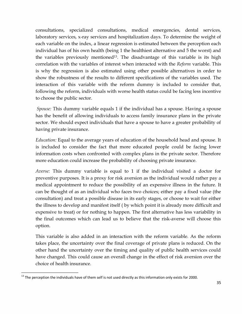
Table 5 shows the division of the total population between the different health
insurance options.
Table 5: Distribution of the Population into types of Health Insurance
2000 %
Public Insurance 77.58
Private Insurance 10.53
Armed Forces 1.84
Other 10.05
2006
Public Insurance 84.84
Private Insurance 7.12
Armed Forces 1.78
Other 6.32
The empirical study only considers household heads that are also formal dependent
workers or pensioners. This group of the population is obliged to use 7% of their wage
or pension to purchase either private or public insurance and therefore cannot choose
not to be insured. The dependent variable of all regressions is a dummy that takes the
value of 1 for individuals with private insurance and 0 for those who have public
insurance. Table 6 shows the distribution of this sub-group between both types of
insurance for each year.
32
Table 6: Distribution of household heads (dependent workers or pensioners) by types of Health Insurance
2000 Total %
Public Insurance 24,069 82.17
Private Insurance 5,224 17.83
Total 29,293 100
2006
Public Insurance 29,154 88.55
Private Insurance 3,768 11.45
Total 32,922 100
Table 6 reveals the interesting fact that the proportion of people with private health
insurance decreased by approximately 6 percentage points during the six year period.
Though 6% seems a small number, it is large relative to the total percentage of people in
the private sector that only amounted to 17.83% in 2000. This strong change only
suggests a possible effect of the health reform as a further analysis of the underlying
change in the choice of individuals is needed. This is discussed in more detail in the
results section below.
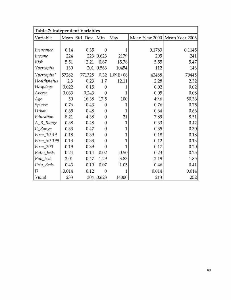
The determining factors of the choice between private and public health insurance are
given by the differences in income, risk, characteristics of the delivery system and
characteristics of the individuals. The variables used and the way they are constructed
is described below, followed by descriptive statistics of each.
Independent variables:
R: This dummy equals 1 in the post-reform year (2006) and 0 in the pre-reform year
(2000).
Risk: This variable is included in order to represent the affiliate’s total health risk, which
partly determines the premium paid for private insurance. Individuals purchase
insurance plans that cover them and their dependents. The law specifies who can be
someone’s dependent. Legally, someone can be a “load” if they are the person’s spouse
or offspring. The latter is valid only until the offspring are 18 years old, or until they are
24 years old but are studying. Other individuals qualify as dependents but only under
33
very exceptional circumstances11. The identification of the individual’s dependents is
the main weakness of this data as it is not directly specified who they are. It is assumed
that the spouse and offspring (under the specified conditions) are dependent on the
household head though it does not consider all the special cases and only considers the
people living in the household. It is however a close approximation to reality, as the
cases not considered are quite exceptional.
The risk index is constructed using a table of risk factors calculated by the Health
Superintendency for different age and gender groups12. The variable Risk equals the
sum of the risk factors of the individual and those dependent on them. These factors
were computed using the estimated expected costs of health services for each group.
Factors indicate the expected costs in terms of health services for each group in relation
to the average cost of all groups. Therefore, a factor of 1 indicates a group with expected
health costs equal to the average. The index has values for men and women of 17
different age groups. The advantage of using this factor table over using the actual
tables that insurance companies use is that the latter would hide a possible change in
the way insurance companies price different levels of health risk. If for example, the
creation of the compensation fund makes it less expensive for insurance companies to
have risky people, this would change the index insurance companies use but not the
index of expected health costs. Therefore the advantage of the index used is that it
reflects the health risk of the individual alone, which is an underlying determinant of
private insurance premiums, and is not affected by changes in the pricing scheme.
The variable is then interacted with the reform dummy to identify the impact the health
reform had on the effect of health risk over the choice of individuals between health
insurance types. The creation of the compensation fund and the reduction in experience
rating should result in the effect of this interaction taking on a positive value toward the
probability of individuals choosing private insurance.
Income: Is the person’s income in thousands of Chilean pesos. This variable is included
in order to represent the price paid for public insurance (7% of this income). It is equal
to the person’s wage or in the case of retirees their pension. For people retired but still
11
Examples of this are: an individual’s parents if they are older than 65 and do not receive a pension, abandoned children under the care of the individual for protection reasons determined by a court of law, abandoned grandchildren and the individuals widowed mother if she has no pension. 12 The study was carried out using values for the 2004. Though factors could be slightly different in the years under study, the illnesses that affect each group and their treatment costs probably did not suffer major changes in such a short period of time. Changes in the types of illness that affect each group, the technology used to treat it and its cost take longer to change significantly the relation in expected health costs between each group.
34
working this income equals the sum of both their wage and pension. It is a truncated
variable as people with monthly income over 60 UF are only obliged to buy health
insurance with 7% of 60UF. A UF was equal to approximately $15,500 pesos in 2000 and
$18,100 pesos in 2006, as it is indexed to inflation. Therefore, this variable is never larger
than 60UF per month in the corresponding year.
If the household head’s spouse is a dependent worker or a retiree, the Income variable
will also include the spouse’s wage or pension. This has an underlying assumption that
the household acts like a nucleus with a single income and with a total number of
beneficiaries. This however assumes that the household head and spouse choose the
same type of insurance. Though this is not always true it has strong advantages. It
reflects the fact that if they both work they will be paying 7% out of their total income if
they choose public insurance. Also, it reduces the problem of assuming children to be
dependent on the household head because it becomes irrelevant if the children are legal
dependents of the spouse or of the household head.
This variable is interacted with the reform dummy to consider possible changes in the
sensitivity of choice to the Income.
The Income variable was constructed to represent taxable income which reflects the price
of public insurance. Per capita income is also added as a control in an attempt to
capture the effect of earnings over choice. Even though both variables have a low
correlation between them, the per capita income control may not stop the coefficient of
Income capturing both the effect of sensitivity to price and sensitivity to earnings. This is
further explored in the results section below.
Ypercapita: Equals the household’s income per capita in thousands of Chilean pesos. It is
added to consider the possibility that the probability of choosing private insurance
grows as income per capita does. The square of this variable is also included in order to
allow for a non-linear effect. Finally, it is also added in an interaction with the reform
dummy as the change in the characteristics of the insurances offered could have
changed the sensitivity of choice to per capita income. Given that per capita income is
constructed using the individuals wage and pension, this variable could be highly
correlated with the Income variable. However, the correlation matrix shown in table 8
indicates a low correlation between both variables.
Healthstatus: This variable is intended to capture the health status of the individual
according to all their information. It is an index constructed as a linear combination of
the amount of health services received in the last three months for: general
35
consultations, specialized consultations, medical emergencies, dental services,
laboratory services, x-ray services and hospitalization days. To determine the weight of
each variable on the index, a linear regression is estimated between the perception each
individual has of his own health (being 1 the healthiest alternative and 5 the worst) and
the variables previously mentioned13. The disadvantage of this variable is its high
correlation with the variables of interest when interacted with the Reform variable. This
is why the regression is also estimated using other possible alternatives in order to
show the robustness of the results to different specifications of the variables used. The
interaction of this variable with the reform dummy is included to consider that,
following the reform, individuals with worse health status could be facing less incentive
to choose the public sector.
Spouse: This dummy variable equals 1 if the individual has a spouse. Having a spouse
has the benefit of allowing individuals to access family insurance plans in the private
sector. We should expect individuals that have a spouse to have a greater probability of
having private insurance.
Education: Equal to the average years of education of the household head and spouse. It
is included to consider the fact that more educated people could be facing lower
information costs when confronted with complex plans in the private sector. Therefore
more education could increase the probability of choosing private insurance.
Averse: This dummy variable is equal to 1 if the individual visited a doctor for
preventive purposes. It is a proxy for risk aversion as the individual would rather pay a
medical appointment to reduce the possibility of an expensive illness in the future. It
can be thought of as an individual who faces two choices; either pay a fixed value (the
consultation) and treat a possible disease in its early stages, or choose to wait for either
the illness to develop and manifest itself ( by which point it is already more difficult and
expensive to treat) or for nothing to happen. The first alternative has less variability in
the final outcomes which can lead us to believe that the risk-averse will choose this
option.
This variable is also added in an interaction with the reform variable. As the reform
takes place, the uncertainty over the final coverage of private plans is reduced. On the
other hand the uncertainty over the timing and quality of public health services could
have changed. This could cause an overall change in the effect of risk aversion over the
choice of health insurance.
13 The perception the individuals have of them self is not used directly as this information only exists for 2000.
36
Given equal individuals, the more risk-averse will probably have a higher probability of
having visited a doctor for preventive purposes. However, the variable has important
shortcomings as it is probably an imperfect measure of risk aversion and only a very
limited number of people visit the doctor for preventive purposes. The variable may
also be affected by other variables as it is subject to the access of individuals to medical
services, the prices of these and the perception individuals have of the probability of
actually being found to be sick if they visit a doctor. The data though does not provide
information which could allow the construction of a more accurate variable.
It is important to bear in mind that though this is an empirical study of a health
insurance system, aversion does not play such a major role as in other studies as
individuals cannot choose to be uninsured. When an individual’s decision to purchase
health insurance is studied, risk aversion becomes one of the most important
determining factors, the case under study however is one of choice between types of
insurance where not purchasing any is not an option and therefore risk aversion plays a
smaller role in determining choice.
Due to the weakness of this variable it is suspected that the Age variable may capture
the effect of risk aversion as older people tend to be more risk-averse.
Age: This variable equals the average age of the household head and spouse. Age is
considered in Sapelli and Torche (2001) as a measure of risk aversion. Given the
previous variable’s possible weaknesses, this one could capture the effect of risk
aversion. It does though probably capture more than differences in risk aversion. It may
also be capturing how older people tend to choose one type of insurance over another
for reasons such as perhaps having greater confidence in public sector health.
For the same reasons as with the previous variable, this variable is interacted with the
reform dummy in order to capture changes in the choices made by the risk-averse.
A_B_Range: Since public sector insurance has different levels of copayments for each
individual according to the group they fall into14, dummies are added to consider these
differences. The lower the copayment rate in public insurance, the bigger will be the
probability of choosing it as the benefits of having it are larger. People who fall into
group A or B make absolutely no copayments for the medical services they purchase if
they have public insurance. Individuals who fall into this group are all those with less
14 Table 15 shows a more detailed description of this division.
37
income than the legal minimum wage or those receiving government pensions or
subsidies.
C_Range: This dummy indicates if a person qualifies to be in group C of public
insurance. People with public insurance that fall into this group pay 10% of the cost of
the medical services they consume. This is the case if the individual’s income is between
one and one and a half times the minimum wage. The omitted group is all those that
qualify to be in group D.
Firm_10-49: As firms become larger it becomes more probable that they will arrange
group plans with private insurance companies for their employees. This increases the
probability that an individual will purchase private insurance. This dummy indicates if
the individual works in a firm with a number of employees ranging from 10 to 49.
Firm_50-199: Equal to the dummy above, but for firms with a number of employees
ranging from 50 to 199.
Firm_200: Indicates if the firm where the individual works in has 200 or more
employees.
Urban: Dummy equal to cero if the individual lives in a rural area, equal to one
otherwise.
Ratio_beds: Is the ratio between the number of private and public hospitals in the
individual’s region.
This variable is included in order to reflect differences in the supply of private and
public hospital services. The use of hospital beds is an imperfect proxy for supply. It is
imperfect as it does not consider the number of doctors or equipment of a hospital nor
how efficient they are in the use of their resources. However, it is probably a good
proxy for supply as it reflects hospital sizes and capacity.
Supply matters as it affects the individual’s utility through several channels15. First of
all, it reduces transport costs as more supply increases the probability of a person being
close to a hospital. Since the number of beds is defined on a regional basis, the variable
Urban is added to account for the fact that private hospitals tend to be concentrated in
big urban areas which means that people living there are more likely to be close to
private hospitals. Supply is also related to the perception of quality of the health service.
Though causality has not been proven, in places where supply is greater quality
15 See Dawes A. & F. Gonzalez (2010) for more evidence on this.
38
indicators tend to be higher. The supply of public health services also determines the
amount of time a patient will have to wait before receiving medical attention. This has a
cost for the individual in terms of his time, but also in terms of his health as a delay in
medical attention can cause an illness to advance more, cause death or reduce the
individual’s quality of life. Long waiting times are a particularly big problem in the
public sector16. The public sector, unlike the private sector, allocates its resources
according not to price but through waiting lists. Where the supply of health services is
greater it is more likely that the hospital will not be saturated and the cost of waiting for
medical attention will be lower. Finally, one of the big benefits of having private
insurance is the possibility of choosing between private providers. The larger the
number of private providers the bigger will be the benefit of having the freedom of
choice.
This variable is added accompanied by an interaction with the reform variable. The
interaction is included because the health reform could have changed the effect that
supply has over waiting times. It is reasonable to believe that the same level of supply
before and after the reform has a different effect on the level of queues. For example, if
the reform increased the demand for public health services, a region that did not
increase its supply will find it has longer queues for medical services than before. The
interaction is included in order to consider this possible effect.
The ratio of the supply is used as the relation between the two sectors may be what is
important to individuals. That would be the case if the level of supply is not as relevant
as the level of supply compared to that of the alternative sector.
A potential criticism to the inclusion of supply variables in the equation is the
possibility of these being endogenous. However, the variables that determine the
decision of increasing supply in a region are probably affected by aggregate preferences
and not individual ones as is the case under study.
Alternative Variables:
The following variables are alternatives to the ones previously defined. They are used to
test the robustness of the results to underlying assumptions or potential problems with
the use of the above variables.
16 As an example of this, the Health Superintendency released a report on the delays in the delivery of health services to patients that showed that some illnesses in the public sector had very high levels of delays. Testicular cancer for example had 38% of medical services delayed. The private Insurers on the other hand had delays in less than 0.5% of illnesses.
39
Hospdays: This variable is added as a proxy of private health information. It is therefore
and alternative to the variable Healthstatus. This dummy takes on the value of 1 if a
person has been hospitalized for more than a week in the past 12 months. This
information cannot be used by private insurers and is therefore private information.
This variable is the one used by Sapelli and Torche (2001) because it has a high
predictive capacity of high future expenditure. Due to the high correlation between the
interaction of Reform with Healthstatus with variables of interest, such as the interaction
of Reform with Risk, Hospdays is used to test the robustness of the results to the exclusion
of Healthstatus.
Pub_beds: Is the number of public hospital beds per 1000 people available in the region.
This variable was obtained using information from the National Statistics Institute’s
(INE) health statistics compendium.
Priv_beds: Is the number of private hospital beds per 1000 people available in the region.
It was constructed using the same compendium as the variable above.
The previous two variables are used to consider the possibility that absolute supply and
not relative supply is what is important to individuals.
D: This dummy variable indicates if the individual’s income is above the maximum
taxable income for private insurance. For individuals in this income range, the price of
public insurance does not vary with income. This variable is used to shed light on the
relative importance of the price and income effect over choice. A further insight of this
is given in the results section.
Ytotal: This variable is equal to the individual’s total income (without considering
restrictions). It is used for the same reason as the previous variable.
Descriptive statistics of the above variables are shown in table 7. It is followed by table 8
which shows the correlation matrix between all independent variables. The interactions
between variables are also included as they concentrate cases of high correlation with
variables of interest.
40
Table 7: Independent Variables
Variable Mean Std. Dev. Min Max Mean Year 2000 Mean Year 2006
Where lit is the error term and all the other variables are explanatory variables included
in Wtli .
β1, β3, β5, β8, β9, β11, β13, β15 and β25 will show the effect of the health reform over the choice
of individuals between private and public health insurance. If these are significantly
different from cero the health reform would have changed the effect the corresponding
variables have over the choice of individuals. Our main interest lies in β3 and β5 as they
will reveal if the health reform actually changed the previous segmentation that existed,
between private and public health insurance, of individuals according to their income
and health risk.
51
VII. Results
The results of all estimations are presented in tables 16-20. Marginal effects are reported
in each case. As a measure of goodness of fit, the pseudo R2 values are also reported as
well as the percentage correctly predicted. The first ranges from 0.35 to 0.45 and the
second borders 0.9 for all regressions. These are relatively high measures of goodness of
fit. Though they may be of some interest, these measures say little about the quality of
the results. The economic and statistical significance of each variable is more interesting
and relevant to the questions under study.
“PROBIT 1” from table 16 presents the main estimates. These are first used to analyze
the effect of the variables of interest, income and health risk, over the probability of
having private insurance. This is followed by a brief insight on other results. The main
specification is then compared to the other alternatives in order to test the robustness of
the results to different specifications, assumptions on functional forms and assumptions
underlying the construction of variables.
Table 10 presents a summary of the findings from the main specification as it shows the
marginal effect of each variable for each year. Table 11 is included in order to illustrate
the significance of these results. It indicates the change in predicted probabilities of
purchasing private insurance for the average individual in response to variations in
independent variables. These variations are equal to one standard error or, in the case of
dummy variables, equal to a change from zero to one. Finally, table 12 is used to further
illustrate the results through examples. It shows the probability that an average
individual would choose private insurance under different scenarios for the year before
and after the reform.
The Income variable, which determines the price of public insurance, has a positive and
statistically significant effect on the probability of choosing private insurance. This is
true for both years, though the effect is smaller for the year after reform
implementation. This is consistent with what was expected, as a higher price of public
insurance should reduce the probability of choosing it. Also, if the variable is capturing
an income effect, the positive effect would be even stronger if private insurance is a
superior good. This possibility is explored further below.
52
Table 10: Probit 1 Marginal Effects for each Year
2000 2006 Mg. Effect p-value Mg. Effect p-value
Income 0.00024 0.00 0.00017 0.00
Risk -0.00544 0.00 -0.00267 0.00
Ypercapita 0.00002 0.19 0.00005 0.00
Ypercapita2 0.00000 0.84 0.00000 0.00
Healthstatus -0.00708 0.35 0.00403 0.45
Averse -0.01478 0.05 -0.00861 0.12
Age -0.00041 0.00 0.00078 0.00
Ratio_beds 0.09908 0.00 0.09480 0.00
Table 11: Changes in Predicted Probabilities of Purchasing Private Insurance for the Average Individual in Response to Changes in Independent Variables.
2000 2006 0→1 ∆Std. Dev 0→1 ∆Std. Dev Difference
Income 0.0662 0.0286 -0.0376
Risk -0.0176 -0.004 0.0136
Ypercapita 0.0047 0.0067 0.002
Healthstatus -0.0019 0.0007 0.0026
Averse -0.0221
-0.0109 0.0112
Age -0.0102 0.0085 0.0187
Spouse 0.0173
0.0078 -0.0095
Urban 0.0175
0.0079 -0.0096
Education 0.0533 0.0014 0.0246 -0.0287
A_B_Range -0.1054
-0.048 0.0574
C_Range -0.0747
-0.0333 0.0414
Firm_10-49 0.0328
0.0155 -0.0173
Firm_50-199 0.0559
0.0272 -0.0287
Firm_200 0.1211
0.0621 -0.059
Ratiocam 0.0182 0.0098 -0.0084
*The change for dummy variables corresponds to a change from 0 to 1. For the rest of the variables the
change corresponds to one from the average value minus 0.5 standard deviations to the average value plus 0.5 standard deviations.
53
Table 12: Examples that Illustrate the Economic Significance of the Regression Results
Variable Value 2000 2006 Difference
Average
0.0814 0.0305 -0.0509
Income 120 0.051 0.017
720 0.400 0.232
∆ 600 0.349 0.215 -0.134
Risk 0.67* 0.128 0.040
9.95** 0.051 0.023
∆ 9.28 -0.076 -0.017 0.059
Age 30 0.094 0.021
70 0.070 0.043
∆ 40 -0.024 0.021 0.045
*Represents the risk of a young single man
** Represents the risk of an elderly couple aged 70-74
The effect of the reform on the marginal effect of income is negative and statistically
significant. This reflects the reduction in the sensitivity of choice to income as public
insurance became more attractive. To see the magnitude of this effect we could simply
look at the coefficient of R x Income and consider that, for an average person the positive
marginal effect of income in thousands of pesos was reduced by 0.00007. To understand
its consequences more profoundly we should look at table 12. Before the reform an
increase in the level of income of 600 ($600,000) from 120 to 720 caused an increase in
probability of 0.349. After the reform the increase in probability is only 0.215, 0.134 less
than before. Though these are examples and the model is a Probit, therefore the effect
depends on the point considered, the change that the reform caused in the sensitivity of
choice to income is far from irrelevant. The reform therefore contributed to a reduction
in the segmentation of the health insurance market by income levels.
A further insight to the magnitude of this effect is given by Figure 3. It shows the
probability of having private insurance for the average individual with different levels
of income. The slope of the post-reform predicted probabilities tends to be smaller;
54
reflecting the decrease in the effect income has on choice. However, the slope is always
positive as more income increases the probability of having private insurance.
Figure 4: Probability of Having Private Insurance for the Average Individual According to Health Risk
Given the previous results, it is possible to conclude that the health reform did have an
economic and statistically significant effect on the insurance market’s segmentation by
individual health risk. The effect risk has on the decision between private and public
health insurance was reduced as those with greater health risk now face lower
incentives to concentrate in the public sector. Figure 4 illustrates the effect of the reform.
It shows the predicted probability that an average individual would choose private
health insurance relative to his health risk. The slope of the predicted probabilities is
56
evidently greater for the pre-reform year, indicating the decrease in the effect health risk
has on individuals’ choice between private and public health insurance. However, the
slope is always negative as more health risk decreases the probability of having private
insurance.
The constant in both years has significant negative effects though in the post-reform
year the negative effect becomes stronger. This change is statistically and economically
significant as it represents a 0.16 change in the probability of choosing private
insurance. This effect could be capturing several factors. The increase in the benefits
offered in public insurance equals an increase in coverage, which translates into public
insurance becoming a more attractive option for all individuals. Also, if there was a
significant change in the quality of the service delivered by health insurance companies,
this would also be captured through this dummy.
As was expected, the health status of the individual has a negative effect on the
probability of having private insurance. Also, the effect of the reform on this coefficient
was positive, which could be because the public insurer no longer acts as a catastrophic
insurer. However neither effect is statistically significant.
The effect of risk aversion on the probability of choosing private insurance was found to
be negative and to decrease after the health reform. This could be related to a reduction
in the uncertainty associated to private insurance plan. However it could also be related
to an increase in the uncertainty over the timing and quality of public health services.
Then again, even if both coefficients have the expected signs, only the one for the pre-
reform year is significant at a 5% level.
The results also indicate that the marginal effect of Age over the probability of having
private insurance is statistically significant for both years. Its effect is negative before
the reform and positive after. Therefore, after controlling for differences in health risk,
before the reform older people had a lower probability of having private insurance than
younger people did and after the reform their probability became larger. Given the
weaknesses previously described of the averse variable, Age could be capturing
differences in levels of risk aversion of older people in relation to younger people,
which could explain the positive effect the health reform had on its estimated
coefficient. Again table 12 is used to quantify the magnitude of the effect. Before the
reform, an average 70 year old person had 0.024 less probability of choosing private
insurance than a 30 year old. After the reform he had 0.021 more probability of having
private insurance. The total difference is 0.045 which is a significant variation.
57
The coefficient for per capita income is not significant in the year before the reform,
though it does have the expected sign. After the reform, the effect is still positive but
significant. However it is so small that even though it is statistically significant,
economically the effect is irrelevant. The square of income per capita follows the same
pattern as it is negative in both years but significant only in the second year.
The ratio between the supply of private and public hospital beds has the expected
positive effect on the probability of choosing private health insurance. Individuals who
live in regions where the relative supply of private hospital services is greater tend to
choose private health insurance more. This could be due to the reasons detailed above
that ranged from effects on perceptions of quality, waiting time, access and the benefit
of variety. The effect in both years is statistically significant, though they are not
statistically different from each other, indicating that the health reform probably did not
modify the effect this variable has on the probability of choosing private insurance.
The rest of the control variables show the expected signs on their marginal effects over
the probability of choosing private insurance. Spouse has a positive statistically
significant effect which could be reflecting the fact that couples can benefit from access
to family insurance plans in the private sector. The average education of the household
head and spouse also has a significant positive effect, which could be a result of more
educated people facing lower information costs when purchasing private insurance.
The fact that an individual lives in an urban zone, and therefore probably has more
access to private providers, has a positive significant effect. Both income ranges have
significant negative effects which could be due to lower copayment rates for these
individuals (in relation to the rest) if they purchase public insurance. The lower the
copayment rate of the group, the larger the negative effect of qualifying for it. Finally,
the size of the firm where the individual works in has a significant positive effect. As
the firm size increases the probability of having private insurance becomes larger.
Though some insights on possible explanations to the marginal effects found for the
control variables are given, it must be taken into consideration that these findings could
simply be reflecting differences in some variable unaccounted for; therefore causality is
not necessarily proven. For example, the marginal effect of living in urban zones could
be reflecting differences in the level of exposure to private insurance propaganda and
information and not necessarily differences in access to private providers. Perhaps
people who marry also have an inclination towards private insurance; therefore the
effect would be due to a selection process and not to the benefit of access to family
plans. More educated individuals could tend to have been previously dependent on
58
individuals affiliated in the private sector and could therefore be more accustomed to
receiving attention in private health sectors, thus leading them to choose private health
insurance with greater probability. These variables are just control variables, which is
the reason why these possibilities are not further explored.
Overall, one of the most important findings of the results is the general decrease in the
probability of individuals choosing private insurance. Table 13 shows the probability of
an individual choosing private insurance for the year before and after the reform. The
confidence interval for this probability is also given at a 95% confidence level. With the
health reform, the probability that an average individual would choose private health
insurance decreased by 0.0509. This is a huge amount if we consider that the probability
was 0.0816 before the reform, therefore it was reduced by more than half.
Table 13: Probability of Purchasing Private Insurance for an Individual Equal to the Sample Average
2000 2006
Probability 95% Confidence Interval Probability 95% Confidence Interval
0.0814 (0.0766 0.0863) 0.0305 (0.0281 0.0329)
Robustness Checks
Table 16 also shows a second set of estimates that follow the same specification as the
first regression. The difference lies in the functional form assumed for the error term
which is now assumed to have a logistic distribution. This regression is estimated in
order to test the robustness of the results to different functional forms. In general, the
marginal effects have the same signs but their magnitude is slightly increased. Since a
different functional form is assumed, different magnitudes can be expected. However,
what is most important is the fact that even if a logistic distribution of the errors were
assumed, the results indicate that the reform had a significant effect in reducing the
negative effect of health risk and positive effect of income over the probability of
choosing private insurance. What is more, these results indicate that if the error term
actually had a logistic distribution, this effect would be even greater than the one
already considered.
With the purpose of analyzing the results subject to changes in the specification of the
equation estimated, table 17 presents 4 different regression results, each of which
included different control variables. The first column presents the simplest specification
as all control variables are excluded and only the variables of interest are considered.
59
The signs and statistical significance of all variables remain the same relative to the
main specification (“PROBIT 1”); the magnitude however is larger for all variables
except the constant. Again this supports our findings as the effect of the reform is found
to be not only significant but larger than that of our main results. This indicates that the
main conclusions are not subject to the inclusion of control variables. The second
column adds the characteristics of the individual such as age, education, level of risk
aversion, health status, zone, presence of a spouse in their household and the
household’s income per capita. Similarly to the previous case, the statistical significance
and sign of the coefficients of the variables of interest remain the same compared to the
main specification though their magnitude is slightly higher in most cases.
Though the variables that determine the decision of increasing supply in a region are
probably affected by aggregate preferences and not individual ones (as is the case under
study) the supply of health services could be considered to be endogenous to the choice
of health insurance. Therefore, the third column from table 17 presents the results for
the probability of having private insurance when the supply of health services is
excluded from the independent variables. The results show no significant change to the
exclusion of supply variables, relative to the main specification, and therefore show the
robustness of the results to this potential endogeneity problem.
Finally column 4 estimates the results allowing for the effect of all variables to change
from one year to another. This specification adds flexibility to the estimation as it drops
the assumption that the coefficients for most control variables remain the same from
one year to another. The risk of doing this is that, if the original specification was
correct, this just increases the variance of the estimated coefficients without gaining
anything in return. The results for the variables of interest show no substantial changes
compared to the main specification. The marginal effects of the interactions of the
reform dummy with control variables are only statistically significant for the education
level and firm size. These effects however are small compared to the variables’ total
effects.
Table 18 presents the results of the estimations of 4 more alternative specifications.
Relative to the main specification, column one excludes the Age variable and column
two excludes the Averse variable. Age has a potential problem related to it. Due to the
fact that health risk increases with age, this variable could theoretically be correlated
with one of the main variables of interest. When Age is interacted with the reform
dummy it indeed has a high correlation with R x Risk. This possibly explains why when
it is excluded, the effect of health risk over choice increases considerably, as well as the
60
change in its effect due to the reform. This suggests that the effect of health risk over
choice from are main specification could be a lower bound. However, this just means
that the effect is still significant but could actually be larger. Compared to the main
results, when Age is excluded from the estimation the marginal effect of Averse grows,
and the same happens to the marginal effect of Age when Averse is excluded. This
suggests that Age may be capturing some of the effects of risk aversion over choice.
Given the weaknesses of the construction of the Averse variable, the results in column 2
allow us to see that the results of the effects of the variables of interest over the
probability of having private insurance are robust to the inclusion of this variable.
The third column from table 17 estimates the main specification after replacing the
Healthstatus variable with the Hospdays variable. This is done because the R x
Healthstatus variable has high correlations with: R x Risk, R x Age, R x Priv_beds and R x
Pub_beds. Hospdays however does not have this problem. The Hospdays variable follows
the same pattern as its alternative since its marginal effect has a negative sign. Also, the
interaction of the reform dummy with Hospdays has a positive though insignificant
effect. Again the results are shown to be robust to the control variables used as the
marginal effects of each variable did not suffer major changes when using a different
indicator of health status.
To consider the possibility that absolute supply, instead of relative supply, affects
individual’s choice between public and private insurance, an alternative specification is
estimated. The results are described in the last column of table 18. Almost all the
marginal effects of each variable remain the same after the specification change, with no
marginal effects changing substantially and with significance levels remaining the
same. Consistent with the previous result, the supply of private hospital beds has a
significant positive effect. This effect does not change significantly after the reform. On
the other hand, the sign of the marginal effect of public supply is positive, which is
contrary to what could be expected. However, this effect is not statistically different
from zero. The effect then becomes statistically significant and negative after the reform.
With the purpose of exploring the robustness of the estimated effect of income over the
probability of having private insurance obtained from the main regression, 2 more
specifications are estimated. The first is presented in the first column of table 19 and it
excludes the Education variable from the main regression. Since individuals with more
education tend to have higher levels of income this variable could be correlated with
the Income variable. The second specification excludes both the Education variable and
the copayment range dummies (A_B_Range C_Range). The latter are related to income as
61
they indicate which income range an individual falls in. As these variables are
excluded, the estimated marginal effect for Income grows, as it is larger in the first
specification and even larger in the second one. This suggests that the estimated
marginal effect of Income from the main regression could be a lower bound. This is also
true for the interaction term between the reform dummy and Income.
The third set of estimates from table 19 tests the robustness of the results to the
assumption that the household head and spouse choose the same insurance type. To
test this, spouses that are dependent workers or pensioners are considered as separate
decision makers. This follows the strategy used by Sanhueza and Ruiz-Tagle (2002). The
results are very similar to those of the main specification and therefore suggest that
assuming that both the household head and spouse choose the same insurance does not
affect the results substantially.
Interpreting the Effect of Income over Choice
The estimations are carried out including both the Income variable and the per capita
income variable. The first is constructed in order to reflect the pricing of public
insurance and the second is included in order to capture pure income effects. However,
it is reasonable to think that the Income variable could be capturing both the effect of
income through price and income itself. The low significance of the per capita income
suggests that this could be the case. Alternatively, it could just be indicating that there is
no pure income effect affecting the choice between types of health insurance.
With the intention of shedding some light on the relative importance of the price effect
and income effect, a strategy used by Cameron and Trivedi (1991) is followed. This
consists of using the individuals for which price does not vary with income to get an
idea of the relative importance of each effect. Since the price of public insurance equals
7% of the individuals’ income with a maximum limit, all those whose income is over
this limit are identified with a dummy variable taking the value of 1 for these
individuals. The main regression is then estimated again using total income (without
limits) and allowing the effect of income to be different for these individuals. The
results of this estimation are given in table 20 and summarized in table 14. The results
suggest that the Income variable is capturing an important income effect. However it is
probably not the only effect it is capturing which is suggested by the statistically
significant difference between the effect of income for those with income over the limit
and below it. This implies that the marginal effects estimated previously for the Income
variable could be interpreted as both the effect of price over choice and income over
62
choice. Both effects are not easily separable as price is a function of income; however
interest lies in the total effect over segmentation which has shown to be significant and
to decrease after the implementation of the reform.
Table14 : Probit 13 Marginal Effects for each Year
2000 2006
Mg. Effect p-value Mg. Effect p-value
Ytotal 0.00024 0 0.00015 0
Ytotal+D_Ytotal 0.00015 0 0.00009 0
Difference 0.00009 0 0.00006 0
Difference/Mg. effect of Ytotal 0.385 0.397
63
VIII. Conclusions
The present study confirmed the findings of previous recent literature that the
segmentation in the market by health risk and income is a result of the coexistence of
two different pricing schemes. Those with higher health risk will have a greater
probability of choosing public insurance and those with higher income will have a
greater probability of choosing private insurance. In addition to this, the findings
suggest that having a spouse, being more educated, working in big firms and living in a
place with a large supply of private health services in relation to public health services
increases the probability of having private insurance. On the contrary, qualifying for
lower copayment rates in the public sector decreases the probability of having private
insurance.
The study’s main contribution is that it identifies a reduction in this effect due to the
implementation of the health reform. In terms of health risk, the implementation of
cross-subsidies and restrictions on experience rating reduced the differences in prices
paid for private insurance. This led to a reduction in the effect of health risk on the
choice between both types of insurance. As public insurance became more attractive
with the reform, the effect of income on the choice of health insurance was also reduced.
In terms of an individual’s choice in relation to their health status, the health reform
was found not to have had a significant impact. Generally, the main conclusion is that
the segmentation by health risk and income due to the coexistence of the two pricing
schemes diminished due to the health reform. Therefore, from the “fairness” point of
view, which disapproves of the concentration of the poor and those who have greater
health risk in the sector with inferior quality health services, this outcome is positive.
However, some people were impacted negatively as would be the case of individuals
who have low health risk and now face a higher price for private insurance because
they are pooled together with the more risky. They must now either pay more or choose
public insurance and thus receive inferior quality health services.
Overall the reform increased the probability of an average individual choosing public
health insurance. The effect is significant as the probability of having private insurance
falls by more than half. This conclusion is important because the reduction in the
segmentation of the market could be viewed as a positive effect and could lead to a
further strengthening of the policies under study, as for example by further increasing
the number of GES illnesses. It is thus important to bear in mind that these measures
will increase the probability of individuals having public insurance which would
64
increase the government’s total burden in terms of subsidies to the public health service
as all these services are subsidized. Also, if the supply of public health services does not
increase simultaneously, the saturation problem of public hospitals will be aggravated.
65
IX. References
Aedo, C. & C. Sapelli. Estudios Públicos; “El Sistema de Salud en Chile: Readecuar el
Mandato y Reformar el Sistema de Seguros”; Vol. 75, (Winter 1999), 189-227.
Cameron, C. & P. Trivedi. Journal of Public Economics; “The Role of Income and Health
Risk in the Choice of Health Insurance”; Vol. 45, (1991), 1-28.
Dawes, A. & F. Gonzalez. “On the Importance of Hospital Supply in Health Reforms:
Evidence from Chile”.
Propper, C. Journal of Public Economics; “Constrained Choice Sets in the U.K. Demand
for Private Medical Insurance”; Vol. 51, (1993), 287-307
Sanhueza, R. & J. Ruiz-Tagle. Journal of Applied Economics; “Choosing Health Insurance
in a Dual Healthcare System: The Chilean Case”; Vol. 5, N° 1 (May 2002), 157-184.
Sapelli, C. Health Care Systems in Developing and Transition Countries: The Role of Research
Evidence; "Risk Segmentation, Moral Hazard and Equity in a Mandatory Health
Insurance System"; Global Development Network, Chapter 5, 2005.
Sapelli, C. & A.Torche. International Journal of Health Care Finance and Economics; “The
Mandatory Health Insurance System in Chile: Explaining the Choice between Public
and Private Insurance”; Vol. 1, N° 2 (Jun. 2001), pp. 97-110
Sapelli, C. & Vial B. Journal of Health Economics; “Self-selection and moral hazard in
Chilean health insurance”; Vol. 22, (2003), 459–476.
Tokman, M., C. Marshall & C. Espinoza. Cepal Serie Financiamiento del Desarrollo; “Un
Matrimonio Difícil: la Convivencia entre un Seguro Público Solidario y Seguros de
Salud Competitivos”; Vol. 199, (December 2007).
66
X. Appendix
IV.1 Explanatory Tables
Table 15 : FONASA copayment rates
FONASA Groups Wage (W) Range Copayment Rate
A People lacking resources or indigent
0%
B W< M 0%
C M ≤ W <1.5*M 10%
D 1.5*M ≤ W 20%
M=Legal Minimum Wage
67
IV.2 Estimation Results
Table 16: Estimates of the Probability of Purchasing Private Insurance (marginal effects reported). Main specification with variation in assumption on functional form of the error term.
(1) (2) VARIABLES PROBIT 1 LOGIT 1
R -0.161*** -2.357*** (0.0316) (0.399)
Income 0.000236*** 0.00410*** (1.08e-05) (0.000168)
R x Income -6.99e-05*** -0.00125*** (1.03e-05) (0.000191)
Risk -0.00544*** -0.102*** (0.000802) (0.0145) R x Risk 0.00277*** 0.0456**