121
Master Thesis in Geosciences 1 The Application of Digital Terrain Analysis for Digital Soil Mapping Examples from Vestfold County, South-Eastern Norway Misganu Debella-Gilo
Master Thesis in Geosciences
1
The Application of Digital
Terrain Analysis for Digital
Soil Mapping
Examples from Vestfold County, South-Eastern Norway
Misganu Debella-Gilo


The Application of Digital Terrain
Analysis for Digital Soil Mapping
Examples from Vestfold County, South-Eastern Norway
Misganu Debella-Gilo
Master Thesis in Geosciences
Discipline: Geomatics
Department of Geosciences
Faculty of Mathematics and Natural Sciences
UNIVERSITY OF OSLO
June, 2007

ii
© Misganu Debella-Gilo, 2007 Tutor(s): Prof. Dr. Bernd Etzelmuller (Geosciences, UiO) Mr. Ove Klakegg (Norwegian Institute of Forest and Landscape) This work is published digitally through DUO – Digitale Utgivelser ved UiO http://www.duo.uio.no It is also catalogued in BIBSYS (http://www.bibsys.no/english) All rights reserved. No part of this publication may be reproduced or transmitted, in any form or by any means, without permission.

iii
Acknowledgement
First of all, I would like to express my deepest felt gratitude to my supervisor, Prof. Dr. Bernd
Etzelmuller, without whose guidance and enthusiastic supervision this thesis would not have been
materialised. He always took his time to discuss with me all the relevant maters and gave me his
utmost advices.
This thesis was done based on data partially obtained from the Norwegian Institute of Forest and
Landscape, the former Norwegian Institute of Land Inventory (NIJOS). I am very grateful to the
institute in general and Mr. Ove Klakegg in particular. Mr. Klakegg has been my external advisor
throughout the course of this thesis work. He was always accessible and ready to arrange the
provision of the data I needed and to discuss with me all the technical matters related to soils. I
am very grateful to him for all of that. My gratitude also goes to Mr. Arnold Arnoldussen, the
leader of the Soil Survey Section of the institute, who was keenly interested in the progress and
outcome of this research and permitted full cooperation of his section for the fruitful completion
of this thesis research.
I would also like to express my gratefulness to the Institute of Geosciences of the University of
Oslo in general and Ms. Marit Carlsen in particular for the comfortable learning environment.
Marit is a study advisor for the M.Sc. and PhD programs of the institute and has always been
cooperative and helpful with me regarding all matters related to my study.
Last but not least, I would like to express my gratefulness to my mother Tirunesh Cheqese and
my father Debella Gilo who made immense sacrifices to keep me in school during my early days
when and where it was rather an exception than the norm to do so.

iv

v
Summary Digital terrain modeling has revolutionized the way topography is characterized and analyzed. Its
applicability has widened to almost anything where topography has a role to play. On the other hand,
digital soil mapping has become the pedological paradigm of the time as it is making tremendous
improvements in the ways soil information is obtained, stored, retrieved and manipulated. This
research was conducted in Vestfold County of south-eastern Norway to use digital terrain analysis
aided by statistical modeling and remote sensing image classification algorithms to make digital soil
maps.
A digital elevation model of 25 meter resolution and digitized soil map of part of the study area
accompanied by data on some analytical properties of soils were used as original data for the terrain
and soil respectively. Fifteen terrain attributes were derived from the digital elevation model through
digital terrain analysis. There were thirteen WRB soil classes in the surveyed area of the study site.
Besides, five most important topsoil properties (the soils content of Clay, Organic carbon, Keldjahl’s
Nitrogen, KNHO3- and pH) for limited number of soil profiles were also used.
The relationship between soil properties and the terrain attributes were analyzed using multiple linear
regression in SPSS. The significant regression models were then fed into ARCGIS to predict the
spatial distribution of the soil properties. The performance of this prediction was evaluated by
comparing it with validation-based ordinary kriging interpolation of the soil properties, which was
conducted in ARCGIS. The prediction of soil classes using digital terrain analysis was conducted
using two conceptually different approaches. First, soil classes were considered as discrete objects
and analysis of variance was used to check if there was significant difference among them in their
terrain attribute values. Then, in analogy with satellite image channels, the terrain attributes were used
as channels and object-oriented supervised classification algorithm was applied in eCgnition by
collecting training areas from the reference soil map. To know the relative performance of this object-
oriented approach, ordinary pixel-based supervised classification was conducted in ARCGIS using
the same training areas. Second, the spatial variation of soil classes was conceptualized as gradual and
fuzzy logic approach was employed for the prediction. Here, the relationship between the soil classes
and the terrain attributes was first modeled using multinomial logistic regression in SPSS to identify
the most influential terrain attributes and to construct logit models for each soil class. The logit

vi
models were used to derive probability prediction models which were then used in ARCGIS to
predict the probability of existence of each of the soil classes as fuzzy variables. The reliability of
this approach was evaluated qualitatively using expert knowledge, empirical soil map of the area and
theoretical background of the soil classes, and quantitatively through correlation study of the
probability values.
The result from the spatial prediction of topsoil properties using terrain attribute showed that the
approach predicted topsoil clay content, KHNO3 content and extractible nitrogen content with better
accuracy compared to the validation-based ordinary kriging. Besides, it showed that about 60% of
each of their spatial variation can be attributed to terrain. On the other hand, insignificant correlation
was found between the terrain attributes and organic carbon content and pH of the soils of the area.
All of the terrain attributes, with the exception of plan curvature, were found significantly influential
in the spatial distribution of soils both by the ANOVA and the logistic regression analysis. Elevation,
flow length, duration of daily direct solar radiation, slope, aspect and topographic wetness index were
found to be the most significant terrain attributes. The crisp approach to the prediction of soil classes
showed that the object-oriented approach performed better than the pixel-based terrain classification
approach. The overall accuracy for the object-oriented approach was 30% while it was only 14% for
the pixel-based. However, the accuracies of some soil classes reached up to 75% in the first approach.
Higher accuracies were obtained for soil classes with higher spatial coverage in the area. The
probability prediction for each soil class using logit models was found to be reliable when evaluated
against the empirical soil maps except for those soil classes which are not greatly influenced by
topography but by other factors such as human activity.
In general, the study revealed that digital terrain analysis has a great potential in digital mapping of
soils and their properties. Fuzzy probability mapping and object-oriented approach were found to be
reliable to a considerable extent in the prediction of soil classes and deserve further research and
application.

vii
Table of Contents Acknowledgement................................................................................. iii Summary ................................................................................................ v
Table of Contents................................................................................. vii List of Figures ....................................................................................... ix
List of Tables.......................................................................................... x 1 INTRODUCTION ........................................................................... 1
1.1 PROBLEM STATEMENT........................................................................................... 1 1.2 OBJECTIVES AND RESEARCH QUESTIONS ...................................................... 2 1.3 SCOPE AND LAYOUT OF THE THESIS ................................................................ 3
2 THEORETICAL AND EMPIRICAL BACKGROUND ............. 6
2.1 THE SOIL-TERRAIN RELATIONS.......................................................................... 6 2.2 DIGITAL TERRAIN MODELLING AND ANALYSIS ........................................... 9
2.2.1 Digital Terrain Modelling ....................................................................................... 9 2.2.2 Digital Terrain Analysis ........................................................................................ 11 2.2.3 Topographic Unit and Automated Terrain Classification ..................................... 12
2.3 PEDOMETRICS AND DIGITAL SOIL MAPPING............................................... 15 2.4 GEOMATICS IN DIGITAL SOIL MAPPING AND PEDOMETRICS ............... 17 2.5 ISSUES OF UNCERTAINTIES IN SPATIAL DATA ANALYSES...................... 19
2.5.1 Uncertainties and Their Sources in Geo-Spatial Analysis .................................... 19 2.5.2 Dealing with Uncertainties .................................................................................... 22
3 STUDY AREA DESCRIPTION................................................... 24 4 METHODOLOGY ........................................................................ 31
4.1 DATA............................................................................................................................ 31 4.2 DIGITAL TERRAIN ANALYSIS ............................................................................. 32
4.2.1 Pre-Evaluation and Pre-Processing of the DEM ................................................... 32 4.2.2 Derivation of Terrain Attributes............................................................................ 33
4.3 TERRAIN ATTRIBUTES AND SOIL PROPERTIES: CORRELATION AND REGRESSION............................................................................................................. 35
4.4 DISCRETE APPROACH TO SPATIAL PREDICTION OF SOIL CLASSES ... 39 4.4.1 Testing Topographic Differences among Soil Classes.......................................... 39 4.4.2 Digital Soil Mapping Using Automated Terrain Classification ............................ 40
4.5 FUZZY APPROACH TO SPATIAL PREDICTION OF SOIL CLASSES .......... 44 4.5.1 Statistical Modelling of the Continuous Relationship between Soil Classes and
Terrain Attributes .................................................................................................. 44 4.5.2 Probability Mapping Using Multinomial Logistic Regression Model .................. 48 4.5.3 Analysis of Reliability of the Probability Prediction ............................................ 49

viii
5 RESULTS....................................................................................... 51 5.1 QUANTITATIVE CHARACTERISTICS OF THE TERRAIN ............................ 51
5.1.1 The Quality of the Digital Elevation Model.......................................................... 51 5.1.2 Digital Characterisation of the Topography of the Area....................................... 52 5.1.3 Interrelationships among the Terrain Attributes ................................................... 54
5.2 RELATIONSHIP BETWEEN TERRAIN ATTRIBUTES AND SOIL PROPERTIES ............................................................................................................. 56
5.2.1 Correlation............................................................................................................. 56 5.2.2 Prediction of Soil Properties Using Multiple Linear Regression .......................... 57
5.3 DIGITAL MAPPING OF SOIL CLASSES AS DISCRETE OBJECTS USING TERRAIN CLASSIFICATION ALGORITHMS .................................................... 62
5.3.1 Analysis Of Variance ............................................................................................ 62 5.3.2 Object-Oriented Supervised Terrain Classification Approach to Digital Soil
Mapping................................................................................................................. 63 5.3.3 Pixel-Based Supervised Terrain Classification Approach to Digital Soil Mapping
............................................................................................................................... 67 5.4 DIGITAL MAPPING OF SOIL CLASSES AS FUZZY VARIABLES................. 69
5.4.1 Multinomial Logistic Regression .......................................................................... 69 5.4.2 Digital Soil Mapping Using Multinomial Logistic Regression............................. 71
6 DISCUSSION................................................................................. 78
6.1 REFLECTIONS ON THE RESULTS....................................................................... 78 6.1.1 Digital Terrain Analysis ........................................................................................ 78 6.1.2 Digital Terrain Analysis and Soil Properties......................................................... 81 6.1.3 Digital Terrain Analysis and Soil Classes ............................................................. 83
6.2 GENERAL REMARKS.............................................................................................. 88 7 CONCLUSIONS............................................................................ 93 8 REFERENCES .............................................................................. 95 9 APPENDICES.............................................................................. 101
ix
List of Figures Figure 2.1 A conceptual view of reality getting blurred by uncertainties (Source: Longley,
2005). ............................................................................................................................. 20 Figure 3.1 The Vestfold County and the study area in relation to the country map of Norway ..... 24 Figure 3.2 The geological map of the study area showing the bedrock types (Source:
Solbakken et al., 2006) .................................................................................................. 26 Figure 3.3 The mean normal monthly precipitation (left) and temperature (right) of the study
area (source: www.met.no).......................................................................................... 26 Figure 3.4 Example profile for three soil classes of the study area: left (Cambisol), Middle
(Histosol) and right (Podzol) (Source: Solbakken et al., 2006)................................... 29 Figure 3.5 Area distribution of the soil classes in the study area .................................................. 30 Figure 4.1 A three by three grid window and the formulae for surface derivatives (modified
from Gallant and Wilson, 2000) .................................................................................. 33 Figure 4.2 Flowchart showing the procedures employed in the object-oriented classification...... 43 Figure 4.3 Graphical depiction of the some of the possible relationship between a predictor
and the class optimality value...................................................................................... 46 Figure 4.4 Flowchart showing the procedures followed in the probability mapping using
multinomial logistic regression models ....................................................................... 50 Figure 5.1 Histograms of the elevation (left) and its aspect (right)................................................ 51 Figure 5.2 Hypsometric curve of the elevation .............................................................................. 52 Figure 5.3 3D visualisation of the topography of the study area................................................... 53 Figure 5.4 Regression predicted clay content versus observed (left) and Kriged versus
observed (right)............................................................................................................ 59 Figure 5.5 Kriging interpolated clay content together with the data sample points (left) and
regression predicted clay map (right). The map covers only part of the study area where profile data were available. ............................................................................... 59
Figure 5.6 Regression predicted versus observed (left) and Kriged versus observed (right) KHNO3- data............................................................................................................... 60
Figure 5.7 Regression predicted versus observed (left) and Kriged versus observed (right) N data............................................................................................................................... 61
Figure 5.8 Separation distance between sample soil classes as plotted against the number of features (dimension) .................................................................................................... 64
Figure 5.9 Map of the soil classes as predicted by object-oriented terrain classification ................ 66 Figure 5.10 Map of the soil classes as predicted by pixel-based supervised classification............ 68 Figure 5.11 Probability Distribution of Albeluvisol (left) and Arenosol (right) ............................ 74 Figure 5.12 Probability Distribution of Anthrosol (left) and Cambisol (right) .............................. 74 Figure 5.13 Probability Distribution of Fluvisol (left) and Gleysol (right).................................... 75 Figure 5.14 Probability Distribution of Histosol (left) and Leptosol (right) .................................. 75 Figure 5.15 Probability Distribution of Luvisol (left) and Phaeozem (right)................................. 76 Figure 5.16 Probability Distribution of Regosol (left) and Podzol (right) ..................................... 76 Figure 5.17 Probability Distribution of Anthropic Regosol (left) and Umbrisol (right) ................ 77 Figure 6.1 A diagram modelling the work flow that might be followed during digital soil
mapping ....................................................................................................................... 92

x
List of Tables Table 4.1 The terrain attributes, their definition and methods of analysis (the symbols are as
given in figure 4.1) .......................................................................................................34 Table 5.1 Statistics for the elevation values ...................................................................................53 Table 5.2 The statistical distributions of each of the terrain attributes ..........................................53 Table 5.3 Correlation Coefficients found among the terrain attributes..........................................55 Table 5.4 Correlation Coefficients and their significance found between terrain attributes and
some topsoil properties.................................................................................................57 Table 5.5 Comparison of the prediction performance of the regression model and validation-
based ordinary kriging..................................................................................................58 Table 5.6 ANOVA result of the soil classes against the terrain attributes .....................................63 Table 5.7 Accuracy of the Object-oriented classification ..............................................................65 Table 5.8 Relationship of the prediction accuracies to other parameters.......................................65 Table 5.9 Pixel-based prediction accuracies ..................................................................................67 Table 5.10 The significance of each terrain attribute in the overall model....................................69 Table 5.11 The influence of each terrain attribute on each soil class as expressed in odd ratios ..70 Table 5.12 The logit models of the soil classes as expressed by the terrain attributes. (Note that
the units are as expressed in table 4.1) .........................................................................71 Table 5.13 Correlation among the probabilities of the soil classes................................................73

1
1 INTRODUCTION
1.1 Problem Statement Digital Terrain Modelling has long replaced the qualitative and nominal characterisation of
topography. It has shown its comparative advantages in that it gives quantitative measurement
of elevation, enables to derive any other terrain attribute quantitatively, enables to visualise
topography in more realistic way than ever before, and enables to store, update, proliferate
and manipulate topographic data digitally (Li et al., 2005; Moore et al., 1993; Wilson and
Gallant, 2000a). It further provides the possibility of deriving indices that can be used as
indicators for environmental processes (Pike, 1988; Wilson and Gallant, 2000b).
On the other hand, the role topography plays in bio-physical processes and phenomena is
increasingly unravelled. One of such bio-physical process is pedogenesis, i.e. the soil
formation process. Due to the fact that topography influences endogenic and exogenic soil
forming factors and processes, it plays crucial role in the spatial distribution of soils and their
properties (Lark and Bolam, 1997; Schaetzl and Anderson, 2005). This is even more so in
high latitude regions such as Norway.
Furthermore, the characterisation and investigation of the spatial distribution of soils and their
properties, i.e. soil survey, is advancing due to the increasing need for knowledge about soils,
triggered by their importance in the environmental well-being and agricultural activities. The
conventional field investigation and laboratory analysis of soils at every site is becoming
increasingly unaffordable in terms of financial cost, time, data deliverability, etc. That is why
other paradigms such as pedometrics and digital soil mapping are widening their scope and
depending their applicability (McBratney et al., 2003).
However, only few countries have made considerable transition to digital soil mapping. What
has become more common is digitizing already available soil maps rather than digital
approach to soil mapping. Norway is one of the few European countries that lack detailed soil
information (Dobos et al., 2006). This might be partly due to the fact that agricultural

2
activities and its environmental consequences are minimal as only 3 percent of the land area is
used for agriculture (Solbakken et al., 2006). However, the rise in demand for detailed
knowledge of soils at relatively low-cost from the public services is triggering the need for
rapid, reliable and updatable soil information system.
Pedometrics and digital soil mapping involve the use of some soil data and auxiliary data on
the biophysical factors such as topography, geology, climate, etc to predict soils and their
properties (Dobos et al., 2006). On the other hand, digital terrain analysis enables to derive
attributes that contain topographic information and indicators for other factors such as
moisture, temperature and radiation implicating that it can provide most of the auxiliary data
needed for the prediction. Such capability of digital terrain analysis and the increasing
demand for reliable and readily distributable soil information make the application of digital
terrain analysis for digital soil mapping a predetermined destiny.
Therefore, this thesis explored those technical possibilities in digital terrain modelling and
demands for, and knowledge gaps in, digital soil mapping to investigate the possibility of
using digital terrain analysis in the spatial prediction of some soil properties and soil classes.
The study was conducted in Vestfold County, southern-eastern region of Norway, where there
are relatively more agricultural activities, more environmental concerns, and where soil
information is consequently more important.
1.2 Objectives and Research Questions The major aim of this research was to make digital map of soil classes and soil properties
through spatial prediction by using digital terrain analysis aided by statistical modelling
and automated classification algorithms. To achieve this major goal, a number of specific
research questions had to be answered. These were:
• Is there correlation between soil properties and terrain attributes? The general concept
that soil properties and topography are related is a long established fact. However, the
particular relationship that exists between a given soil property and a given terrain
attribute is complicated because it varies across space and over time. Besides, the
quantitative relationship is a relatively less studied matter. Thus, the aim here was to

3
study the relationship between some topsoil properties and terrain attributes
quantitatively.
• Is it possible to spatially predict soil properties from terrain attributes? To tackle the
expensive and time consuming measurement of soil properties at every site, predictive
approaches are used very often. Most of the known predictive methods are
interpolation (such as kriging) and pedotransfer functions that enable to derive one soil
property from others. But, the question here was: If the relationship between terrain
attributes and soil properties could be established, isn’t it possible, and even better
than the other approaches, to predict soil properties from terrain attributes?
• Are different soil types located under significantly different terrain characteristics? It
is not just the soil properties that are known to be affected by topography, but the
general soil type as well. However, what are the particular terrain attributes that
significantly vary with soil types, at least for the particular study area?
• Is it possible to spatially predict soil types as discrete objects using automated terrain
classification? Here, soil classes were perceived as discrete objects with spatially
defined boundaries. The aim was then to know if these spatial soil objects could be
related to terrain objects and if they could be predicted through classification of the
terrain into soil-terrain objects using automated classification algorithms.
• Is it possible to spatially predict soil classes as fuzzy variables using digital terrain
analysis? Refuting the notion that soil classes are discrete objects, this research
question tried to address the issue of within soil unit uncertainty and approach the
problem from the concept of gradual variation. The research goal here was then to
predict the probability of the existence of a soil class at every site using digital terrain
analysis aided by statistical modelling.
1.3 Scope and Layout of the Thesis The springboard of this research was that since topography is known to have central role in
influencing the existence, type and characteristics of soils, it is possible to quantitatively relate
topographic attributes to soils and their properties and predict the spatial distribution of the
later (McKenzie and Ryan, 1999; Thompson et al., 2006; Thwaites and Slater, 2000). The
foundation of this principle is the morphometry-process relationship, which shows that

4
surface processes are influenced by shape and size, i.e. morphometry, of the terrain
(Etzelmüller and Sulebak, 2000).
The specific research questions of the thesis were as explained in the objectives section.
However, its ultimate focuses were derivation of primary and secondary terrain attributes to
fully and quantitatively characterise the topography of the area and to be able to make digital
maps of soils and their properties based on just terrain information. Therefore, why and how
the soil classes were created in the study area was not the focus of the study. It rather paid
great deal of attention to as to how soils could be digitally mapped using terrain information
and limited empirical soil information. It is well known that prediction of soil requires
information on all soil forming factors. This research was not conducted with ignorance of
that. It was rather aimed at determining how far one could go in using detailed terrain
information to predict soils since the influence of other factors might, at least partly, be
covered by terrain information. The lay out of the thesis is as follows.
The first chapter briefs the reader with the problem statement. It provides the background and
the problems that led to this research idea. Besides, it states clearly what the objectives of the
research were. This was supplemented by the research questions that this study tried to
answer.
Chapter two explores the theoretical and empirical background of the research theme. It gives
brief overview of the relationship between topography and soils after defining the two
entities. It further explains the principles of digital terrain modelling and analysis. The chapter
also introduces the most recent paradigms in soil survey, i.e. pedometrics and digital soil
mapping. The roles that geomatics could play through its tools and techniques in digital soil
mapping in particular and pedometrics in general have also been visited in this chapter. Since
no geo-spatial analysis is without error, issues of uncertainties such as their sources and
methods of estimation have also been explored in this chapter. This chapter is followed by
Chapter three which introduces the study area. It describes the location, geology, climate, land
use, and soils of the area briefly giving more attention to the definition of the soil classes of
the area.

5
Chapter four gives detail step by step explanation of the methods and procedures used in this
research. It starts with explaining the data set used and goes on by discussing the methods
applied to tackle each of the research questions. Brief quantitative description of the methods
is also given where necessary.
Chapter five presents the results of the research which includes tables, graphs, maps and text
that explain the results of the study. It begins by giving quantitative characterisation of the
terrain together with the uncertainties involved in the digital terrain modelling. The
relationship between soil properties and terrain attributes follow with the prediction of the soil
properties from terrain attributes. The prediction of soil classes from terrain attributes has
been divided into the discrete and fuzzy approach. Accuracy estimates and reliability
evaluation accompanied each result.
Chapter six gives explanation and reasoning to the results by connecting to theoretical and
earlier empirical findings. The chapter is divided into two main sections. The first one
reflects on the results focussing on the digital characterisation of the terrain, terrain and soil
properties, and terrain and soil classes. The second section adds some general remarks that
tried to connect the research outputs with practical applications.
Chapter seven concludes the whole thesis by extracting the main facts obtained from this
study. It tries to answer the research questions posed in chapter one. The appendix and the
CD-ROM attached give other information that could not be included in any part of this thesis
but are believed to be of interest for the reader.

6
2 THEORETICAL AND EMPIRICAL BACKGROUND
2.1 The Soil-Terrain Relations
The soil topography relation is best understood when the two entities are defined first. Soil
can be defined as the unconsolidated mineral or organic material on the surface and
immediately beneath the surface of the earth that serves as a natural medium for the growth of
land plants, that has been subjected to and shows effects of genetic and environmental factors
of climatic, macro-and micro-organisms, conditioned by relief, acting on parent material on a
period of time (USDA’s NRCS: http://soils.usda.gov/education/facts/soil.html). This
definition of soil by itself acknowledges the statement by Jenny (1941) that soil varies over
space and time and is influenced by a range of environmental factors such as parent material,
climate and topography.
Topography, sometimes known as landscape or relief, is a crucial factor in soil genesis
because, with the exception of time, it modifies the role that the three other factors play in soil
genesis (Brady and Weil, 2002). But, what exactly is topography? Hugget and Cheesman
(2002) define topography more or less as the general configuration of the land surface and sea
floor, including its relief and the location of its features, both natural and human-made.
Basically it is described by locational and structural attributes. The main locational attributes
are latitude, longitude and altitude. Where as, the structural attributes define the form of the
land and are direct or indirect derivatives of the locational attributes. The major ones of them
are slope, aspect, plan curvature, profile curvature, etc.
Topography plays both direct and indirect roles in surface and subsurface biophysical
processes through its locational and structural attributes (Bell et al., 2000; Hugget and
Cheesman, 2002; Wise, 2002). The direct impacts of the locational attributes becomes greater
at greater scales such as regional and global, where as that of the structural attributes is
already considerable at miner scales, especially at the toposcale (Burrough et al., 2001). All

7
the discussions in this thesis with regard to topographic influences on soil are, therefore,
implicitly at toposcale as the study is focused on the structural attributes
When a closer look at pedogenesis, i.e. soil formation process, and the role of each of the five
environmental factors is taken, the soil-topography relation becomes more apparent.
Investigation of the researches conducted on soil topographic relations (Crave and
GascuelOdoux, 1997; Manning et al., 2001; McKenzie and Ryan, 1999; Webb et al., 1999;
Webster, 2000), leads to the following three points which will become clearer with the
subsequent discussions:
• First, topography dictates whether soil develops or does not develop at a given space;
• Second, if it develops, topography dictates the type of the soil;
• Third, even if the general soil type might be the same, topography affects the
individual properties of the soil.
The first desirable condition for a soil to develop at a given space is the presence or absence
of parent material (Brady and Weil, 2002; Schaetzl and Anderson, 2005). Decomposable
organic material and/or weatherable inorganic materials have to first deposit in the area. This
deposition takes place only if the topographic characteristics are suitable for deposition.
Otherwise, the place may become a source of parent material for other places, itself being an
erosion area. Once the parent materials start to deposit, pedogenic processes start to act on
them. The type and the rate of these pedogenic processes are determined by environmental
factors such as climate and organisms. Besides, just like any other process, pedogenic
processes advance with time (Brady and Weil, 2002; Schaetzl and Anderson, 2005).
When we take the case of climatic influences, the major climatic components that play
considerable role are precipitation, temperature and solar radiation as they influence
decomposition of organic materials and weathering of minerals (Brady and Weil, 2002;
Schaetzl and Anderson, 2005; Wakatsuki and Rasyidin, 1992). The spatial distribution of
moisture and duration for which it prevails at a given space is dictated by the topographic
characteristics of the area. The energy that comes from the sun, that is the source of radiation
and heat, is not evenly distributed spatially and temporally. Its spatial distribution is related to

8
the locational and structural attributes of topography (Hugget and Cheesman, 2002). This
local variation in temperature, radiation and moisture regimes due to topography creates a
kind of micro-climate (Hugget and Cheesman, 2002; Wilson and Gallant, 2000a)
Presence or absence and the type of macro- and micro-organisms, which are influenced by
climatic conditions, influence the rate with which soils are formed, the type of soils that
develop and the individual properties of the soils (Brady and Weil, 2002; Schaetzl and
Anderson, 2005). The climatic and organic factors of soil formation are intertwined and are
highly dictated by both the locational and structural attributes of topography. Consequently,
other things being equal, 0the soils that might develop under the same macro-climatic zone
vary immensely due to the fact that topography modifies climate and create a sort of micro-
climate (Tromp-van Meerveld and McDonnell, 2006).
Most topographic attributes play significant role directly or indirectly in soil development as
summarized by some researchers (Schaetzl and Anderson, 2005; Tromp-van Meerveld and
McDonnell, 2006). All other things kept uniform, soils develop faster and deeper in flat areas
compared to steep areas as their moisture regimes are favourable and materials tend to
accumulate in flat areas but move away from steep areas. On the other hand, aspect modifies
the influence of slope by exposing or obscuring the slope to and from solar radiation dictating
the temperature and the moisture regimes. Curvature is as important as the slope because the
concavity and convexity of the sloping area governs the storage and flow of water and solid
materials over the slope.
Of the soil properties that vary spatially with topographic attributes, solum depth, horizon
thickness, texture, moisture content, organic matter content, nutrient content, etc are the most
important ones (Manning et al., 2001; Tromp-van Meerveld and McDonnell, 2006). The
specific relationship between terrain attributes and soil properties is an issue still under
continuous study. More precisely speaking, the quantitative functional relationships between
terrain attributes and individual soil properties have not yet been established.
9
The fact that topography influences soil formation and soil properties has led to the
development of the concept called the soil-landform model, .i.e. the soil catena or the soil
topo-sequence (Schaetzl and Anderson, 2005). The concept is based on the principle that the
continuous spatial variation of topographic features leads to a continuous spatial variation of
soils, i.e. the soil continuum. The concept is complicated by the fact that soils are influenced
by at least four other major factors than topography. The concept has, nonetheless, been
helping in soil survey tasks. It has even been evolving to quantitative approaches and has
consequently been part of the theoretical springboard of this research.
2.2 Digital Terrain Modelling and Analysis
2.2.1 Digital Terrain Modelling
In order to understand topography and its role in environmental processes and phenomena,
there needs to be a technique for measuring, representing and characterising it reliably. On the
other hand, measurement, representation and characterisation of such a vast and continuous
feature are very challenging. Therefore, there needs to be a technique whereby the complexity
is simplified and the vastness is scaled down. Such an objective is achieved through
modelling. Modelling involves simplification and scaling down of reality to a
comprehendible level with relative ease (Li et al., 2005).
There are many ways of modelling terrain, such as descriptive, pictorial, cartographic,
physical and digital. Descriptive method simply involves describing topography using
nominal terms of topographic parameters such as hills, hillslopes, valleys, concaves,
convexes, undulating, steep, gentle, etc. The reality is then modelled only through mental
perception. Pictorially, in the early days, painting was used to represent topography and
accompanying features. Cartographic maps were later used for the same purpose especially
with the invention of the topographic maps in the form of contours in the nineteenth century
(Li et al., 2005). Physical modelling of topography is representation of terrain by physical
objects as it is often used in the military. Digital modelling involves virtual realisation of
terrain using computers (Li et al., 2005; Wilson and Gallant, 2000a).

10
An ideal terrain model is the one that can fully represent the reality of terrain. Although this is
practically not possible to achieve, a good terrain model should have some desired qualities
(Li et al., 2005; Pike, 1988; Wilson and Gallant, 2000a). First, it has to be able to give the
perspective view of the physiography. Second, it has to be based on quantitative
measurements. Third, it has to enable further quantitative analyses. Fourth, it should not be
too complicated and too demanding. Fifth, it has to be duplicable and replicable. Such
qualities are achieved through digital modelling since each of the others lack one or more of
such qualities. As a result, the most common way of storing topographic information has now
become the Digital Terrain Model (DTM) where elevation values, stream lines and other
related terrain attributes are digitally stored together with their locational attributes (Li et al.,
2005; Moore et al., 1993; Wilson and Gallant, 2000a).
The structure with which elevation is modelled digitally varies, and it has gone through
transformations. Basically, there are three well-known data structures for terrain modelling
which are explained in detail in (Hutchinson and Gallant, 2000; Li et al., 2005; Moore et al.,
1993; Smith, 2005). The first one is the more traditional contour maps in which case elevation
values are represented by isolines, i.e., lines connecting points of equal elevation values of
fixed intervals that are digitized, stored and used to model topography. However, due to a
number of reasons it is less favoured and less often used in digital terrain modelling although
it is the most widely available terrain data source. It underrepresents areas between the
contour lines. It is little suitable for further analysis. And, it is incompatible with other
geographical data structures.
Another structure with which DTM represents topography is the Triangular Irregular Network
(TIN). TIN is created by constructing a triangulation of the elevation data points, which form
the vertices of the triangles, and then fitting local polynomial functions across each triangle
(Wilson and Gallant, 2000a). This creates a very good result for visualization, requires less
storage space and seems to represent the terrain more closely. However, triangulation
methods are sensitive to the positions of the data points and the process needs to be
constrained to produce optimal result. Besides, due to its rigidity in further analysis and its
incompatibility with other spatial data structures it is less widely used.

11
The most widely favoured structure is the raster model where elevation values are represented
by square grids of fixed size. This is easily used for further analysis and easily integrated with
other spatial data structures (Hutchinson and Gallant, 2000; Moore et al., 1993; Wilson and
Gallant, 2000a). This also does not come without drawbacks. First, the size of the grids often
affects the storage requirements, computational efficiency and the quality of the result.
Second, square grids can not handle abrupt changes in elevation easily, skipping important
details. Third, the within grid variation is simply ignored.
The outcome of any model is dependent upon the original data that is used for the modelling.
DTM is not an exception. The tools used for the capturing of numerical terrain data, too, have
gone through tremendous progress (Hutchinson and Gallant, 2000; Wilson et al., 2000).
Ground measurement of locational variables and some structural variables such as slope have
been practically inadequate to cover large areas. The use of aerial photographs for civilian
purposes brought in the art of photogrammetry as a tool for the measurement of topographic
parameters. This technique has widely been used to capture topographic information at
national levels around the world. However, the need for more accurate, faster, cheaper,
reliable and repeatable method that can provide ready made numerical topographic
information with global coverage has triggered the search for more advanced technologies. As
a result, other air-borne and space-borne technologies have been brought in. To mention a
few of such techniques: space borne optical satellites that employ photogrammetry, airborne
radar and space-borne radar technologies that employ interferometry, airborne Lidar
technology, global positioning system, etc. Although the desired qualities have not yet been
achieved, they are on the progressive direction (Li et al., 2005) .
2.2.2 Digital Terrain Analysis
The mathematical analysis of terrain information including the derivation of the surface
elevation data using computers is known as digital terrain analysis (Li et al., 2005; Pike
Richard, 2000). In digital terrain analysis, the digitally stored elevation and other topographic
features are used to derive other terrain attributes. The derivation of other attributes from

12
elevation values is a follow up to the conversion of terrain information into a spatially
connected surface data through interpolation or filtering depending on the data source (Li et
al., 2005; Moore et al., 1993).
The terrain attributes are grouped into primary and secondary (Moore et al., 1993; Wilson and
Gallant, 2000a). The primary terrain attributes are those which are directly derived from the
elevation values, where as secondary terrain attributes, sometimes known as compound
attributes, are those that are derived through functional combination of the primary terrain
attributes. The main primary terrain attributes are surface derivates, slope, aspect, plan
curvature, profile curvature, upslope contributing area, etc. The definitions and the ways they
are derived are explained in depth by (Gallant and Wilson, 2000; Li et al., 2005; Moore et al.,
1993) and are presented in table 4.1.
The terrain attributes so derived can be used to derive topographic indices that are indicators
of pedological, geomorphological, hydrological, ecological and other surface and subsurface
processes(Pike Richard, 2000; Wilson and Gallant, 2000b). These indices, i.e. the secondary
topographic attributes, include topographic wetness index, sediment transport capacity index,
the stream power index, the solar radiation index, etc. Their definition and methods of
derivation are thoroughly discussed by (Moore et al., 1993; Wilson and Gallant, 2000a).
Besides, both the primary and the secondary topographic attributes can be used to predict
surface and subsurface processes. Derivation of both the primary and secondary terrain
attributes is most often conducted using GIS tools based on the raster data structure.
2.2.3 Topographic Unit and Automated Terrain Classification
The fact that most of the environmental processes that take place on the surface of the earth
vary with topography (Etzelmuller et al., 2001; Hugget and Cheesman, 2002; Moore et al.,
1991), leads to the hypothesis that if processes vary when topography varies, they should
remain uniform when topography is kept uniform. This leads to the goal of finding a unit in
which topographic attributes do not vary significantly, and implicitly surface processes do not
vary significantly as well.

13
The terms used for such a unit are many and confusing. Names such as landform unit,
landscape element, landform element, land element, facet, etc are used. For example, Hugget
and Cheesman (2002) used landform unit and landform element interchangeably and defined
it as simply-curving geometric surfaces lacking inflections and are considered in relation to
upslope, down slope and lateral elements. They also state that landform element is the same as
facet and land element. Schmidt and Hewitt (2004) also define land element as small areas of
land surface that are uniform in geomorphometric parameters such as slope, surface
roughness, contour and profile curvature. Therefore, terms such as landform unit, landform
element, land element and facet are geomorphometrically defined and are more or less the
same.
Whatever the name might be, the idea here is to find a fundamental unit over which
topographic variables, and implicitly surface processes too, do not vary significantly.
However, it is known that most spatial processes and topographic attributes are continuous by
nature and there is difficulty in setting boundaries. Although terrain is naturally continuous,
discretisation simplifies the complication of the topographic attributes by using statistically
set boundaries. The fact of the matter is that it is generally possible to create topographic unit
using mixture of any of the topographic attributes. The question, however, is getting the
topographically uniform unit which also indicates uniformity in process, i.e. form-process
relation (Etzelmüller and Sulebak, 2000). If that is possible to identify, it might help to
indirectly map processes through mapping topography.
Terrain classification has long been based on the qualitative description of the topographic
attributes and the classes are also only of qualitative and nominal nature. Recently, the
development of digital terrain analysis in GIS offered opportunity for quantitative and
automated classification of terrain. As mentioned previously, topography is a continuous
physical variable. Automated quantitative terrain classification in GIS provides the possibility
of approaching the continuous nature of terrain in two ways. The first is classifying terrain
into spatially discrete topographic units as stated earlier. The second approach is fuzzy
classification to simulate the continuous reality of topography. In fuzzy classification terrain

14
units may not be categorised into one terrain class, they are rather assigned with membership
value expressing how much they belong to the given class (Schmidt and Hewitt, 2004).
Empirical attempts show that the outputs of terrain classification are dependent upon the
algorithm used and the statistical rules set for the algorithms. Irvin et al. (1997) and Ventura
and Irvin (2000) classified terrain into uniform units by applying the iso-clustering
unsupervised classification algorithm using six terrain attributes as classification criteria. The
result indicated that automated numerical classification classified terrain into more detail than
the conventional qualitative method does. Moreno et al. (2005) also classified terrain
automatically using GIS into land elements based on geomorphometry and concluded that it is
less time consuming with a rewarding result compared to manual delineation of land
elements, yet with unnecessarily too much detail. Such too much detail can be of advantage
when further analysis is needed.
On the other hand, there are continuous classification attempts made based on the fuzzy logic
theory (Irvin et al., 1997; Schmidt and Hewitt, 2004; Ventura and Irvin, 2000). In fuzzy
classification topographic units are predefined and the whole area is classified based on
numerical membership of each grid to each of the units. Therefore, a map is created for every
landform unit depicting membership probability values of each pixel. Continuous
classification provides more information about the character and variability of the topography
compared to iso-clustering and manual delineation.
The advantages of the automated quantitative terrain classification over the conventional
qualitative method are that: it can be more accurate if the data and parameters used for the
classification are accurate, it can be used for quantitative studies of the relationship between
topography and surface processes, it can easily be integrated into GIS, and it is readily
transferable and interpretable. However, in both the discrete and continuous classification, the
terrain attributes to be used as criteria for the classification have not yet been standardized.
Besides, the terrain classes are expected to show some sort of process classes. The validity of
the classification is thus dependent upon its ability in connecting to the variations in surface
processes that are known to be affected by topography.

15
2.3 Pedometrics and Digital Soil Mapping
Soil is a thematically complex, spatially mosaic and temporally dynamic environmental
variable. Therefore, ideally, its knowledge necessitates measurement of all soil properties,
across all spaces continuously or periodically. However, reality does not allow such tasks due
to technical, economical and logistic limitations. Consequently, what is practically possible is
the measurement of some soil properties at selected sites at a given time or periodically. The
big question is, then, how can we have knowledge about the rest of the soil properties at all
other sites? Besides, how can we monitor them across time?
To tackle the above fundamental problems, researchers have come up with different
approaches over time. By quantitatively modelling the relationships among the numerous soil
properties, unmeasured soil properties could be predicted through pedotransfer functions
(Shein and Arkhangel’skaya, 2006) thereby reducing the thematic complexity issue. Besides,
spatial prediction of soil properties is most often dealt with through the combination of
approaches such as interpolation, geostatistics and predictive modelling (Goovaerts, 1999;
McBratney et al., 2000). Only few very dynamic soil properties such as soil moisture content
and temperature are temporally monitored (Kang et al., 2000; Romano and Palladino, 2002).
That might be due to the fact that the time span for the dynamism of some soil properties is
too long for human life and that of others is too short and thus demand much material, time,
finance and technique.
Most of the above approaches employ quantitative methods and deal with prediction, one way
or another. Quantitative pedology was first proposed by Hans Jenny in the early 1940’s
(Jenny, 1941), although it peaked momentum in the 1960’s. Such approaches have recently
been re-disciplined under the umbrella of pedometrics. Pedometrics is defined as the
application of mathematical and statistical methods for the study of the distribution and
genesis of soils (Burrough, 1994). The term is analogous with geometry encompassing two
Greek words, i.e. pedo means soil and metrics refers to measuring. The approaches of

16
pedometrics are mathematical and statistical instead of the conventional field survey and
qualitative modeling (Burrough, 1994; McBratney et al., 2000).
Any kind of spatially variable environmental object is best described through mapping.
Mapping is a medium of communication that is concise, explicit and implicit at the same time.
Soil is one of such environmental objects perceived as spatially variable. Consequently, soil
mapping is an integral part of soil survey. There is a discipline called soil geography
(pedogeography) that focuses on the location, distribution and pattern of soils on the
landscape (Scull et al., 2003). However, the conventional approaches to soil geography have
a number of drawbacks that needed to be dealt with. First, they rely on field observation and
laboratory data on soils and their spatial extent, which are costly and slow to acquire (Schuler,
2006). Second, the outcomes have mostly been produced as paper maps which are not easily
stored, replicated and distributed, and thus lack the quantitative aspects needed for
interpretation and further uses. Third, in almost all cases, soil classes are treated as discrete
objects and the spatial continuity of soils is not often taken into consideration.
Dealing with the above drawbacks of conventional soil mapping, the quantitative and
predictive approaches of pedometrics combined with the advancements in the analytical
capabilities of computers triggered the birth of digital soil mapping. Digital soil mapping has
achieved such a global attention that a global working group that deals with promoting the
approach has been setup (http://www.digitalsoilmapping.org). The European branch of this
working group defines digital soil mapping as follows:
Digital soil mapping is the computer-assisted production of digital maps of soil type and
soil properties. It typically implies use of mathematical and statistical models that
combine information from soil observations with information contained in correlated
environmental variables and remote sensing images (Dobos et al., 2006).
In digital soil mapping, observed soil data and auxiliary data are integrated to predict soil
properties and soil classes. The observed soil data may include soil profile description,
laboratory data and soil classification. On the other hand, auxiliary data may include terrain
parameters, remote sensing images, soil and other auxiliary maps. These are needed because

17
soil mapping generally requires predefined model of soil formation and data on soil properties
and other environmental variables that have significant impact on soil formation and thus on
the spatial distribution of soils and their properties (McBratney et al., 2003). Nonetheless,
digital soil mapping has advantages over digitizing soil maps as it avoids or minimizes the
lengthy and costly procedures of field investigation and laboratory analysis.
There are different and numerous tools used in digital soil mapping. These are state-factor
models, pedotransfer functions, geostatistics, statistically set empirical models, discrete and
fuzzy classification, decision trees, artificial neural networks, etc (Behrens and Scholten,
2006; McBratney et al., 2003). Behrens et al. (2005) used artificial neural network to digitally
map soil classes based on the digital data of geology, terrain and land use. They concluded
that using data on relief, land use and geology artificial neural network has a very high
predictive power. Behrens and Scholten (2006) reviewed digital soil mapping in Germany and
state that the approach is reliable and can be used intensively. There are also other researches
done on spatial prediction of soil properties such as organic carbon (Ping and Dobermann,
2006; Simbahan et al., 2006), pH, nitrogen, carbon, Phosphorous and clay content (Henderson
et al., 2005). They also came up with encouragingly satisfactory results. However, since the
approach is relatively new methodological aspects have not been well explored yet. Besides,
only few selected terrain parameters were used in most of these studies. There needs to be
inclusion of as many parameters as possible in the analysis. Besides, more predictive
approaches need to be explored.
2.4 Geomatics in Digital Soil Mapping and Pedometrics Dealing with spatial data needs tools that are well advanced in capturing, storing and
analysing spatial data. That is just what geomatics is capable of doing. Geomatics is the
discipline of gathering, storing, processing, and delivering of geographic information, or
spatially referenced information (http://en.wikipedia.org/wiki/Geomatics#Overview). Due to
such capabilities, geomatics plays central role in pedometrics in general and digital soil
mapping in particular.
Techniques and tools employed by geomatics that are relevant to pedometrics and/or digital
soil mapping are digital terrain analysis, remote sensing, Global positioning system,

18
geostatistics, spatial analysis, etc. Global positioning system and remote sensing provide
information about some of the environmental factors and their positions on the surface of the
earth. Geostatistics and spatial statistics are tools used to establish and study the relationships
among soil properties and between soil properties and environmental factors. On the other
hand, digital terrain analysis provides data and analytical capabilities with respect to one of
the most crucial environmental factors that influence soils and their properties, i.e.
topography.
Of those tools used in geomatics, digital terrain analysis stands out because it is relevant to a
well established conceptual model in pedometrics, i.e. the soil-landscape model. Earlier it has
been discussed that primary and secondary topographic attributes can quantitatively be
derived in geomatics through the process of digital terrain analysis. This terrain attributes are
interesting because they affect soil development and other surface and subsurface processes
(Etzelmuller et al., 2001; Florinsky et al., 2002; Moore et al., 1993; Wilson and Gallant,
2000a).
The terrain attributes in particular and digital terrain analyses in general are widely used in
soil-landscape modeling which is central in spatial prediction of soils and their properties.
Some of the applications include prediction of soil moisture content (Blyth et al., 2004;
Romano and Palladino, 2002; Sulebak et al., 2000) soil moisture deficit (Krysanova et al.,
2000), level of water table (Rodhe and Seibert, 1999), soil organic carbon content (Bell et al.,
2000; Florinsky et al., 2002). The case studies indicate that the performance of digital terrain
analysis in predicting soil properties seems to depend on the terrain attributes used, the
algorithms employed and the types of landscape on which the application is conducted.
Earlier the concepts of topographic units and automated terrain classification have been
briefly explained. These concepts are very relevant to digital soil mapping. For long time,
landscape classification has been used to define soil spatial units (Bartsch et al., 2002; Dragut
and Blaschke, 2006; Hengl and Rossiter, 2003; Irvin et al., 1997; Ventura and Irvin, 2000).
Geomatics with its possibility of dealing with spatially continuous quantitative data offers the
opportunity of classifying terrain into either discrete units or fuzzy memberships. Besides, it
offers the opportunity of quantitatively relating spatially variable attributes to soil properties.

19
Many of the case studies that tried to delineate landscape unit through terrain attributes have
come up with encouraging results (Etzelmuller et al., 2001; Ippoliti et al., 2005; Irvin et al.,
1997; Park et al., 2001; Schmidt and Hewitt, 2004; Schmidt et al., 2005). The results have
shown that topographic units that are delineated by using terrain attributes implied either
homogeneous units in certain aspects such as soil properties or even homogeneous soil
classes.
Review of the theoretical principles and empirical evidences has shown that geomatics plays
crucial role in quantitative prediction of soils and their properties. This might even lead to the
evolution of a unique branch of soil geography, i.e. pedogeomatics? Pedogeomatics could be
defined as a technique whereby spatially referenced data on the environmental factors of
pedogenesis are gathered, stored and processed quantitatively to predict the spatial
distribution of soils and their properties. This research deals with a part of this theme.
2.5 Issues of Uncertainties in Spatial Data Analyses
2.5.1 Uncertainties and Their Sources in Geo-Spatial Analysis
It has been recognised from the early days of modern science dating back to over three
centuries that representation of realities through measurement and modelling seldom fully
duplicate the reality (Rouvray, 1997). That means scientific analyses are seldom free of
uncertainties. Uncertainties in geo-spatial analyses are recognised to be significant and are
likely to be just as important as the estimated or simulated outputs (Atkinson, 1999).
There are a number of confusing terms related to the indicators of the (mis)representation of
reality such as error, uncertainty, accuracy, precision, quality, vagueness, fuzziness, etc. One
thing they have in common is that they express the correctness or non-correctness of the
representations of reality. Even though the terms mentioned above have some differences,
most scientific articles do not make clear distinction among most of them. Wechsler and Kroll
(2006) define error as the departure of a measurement from its true value. They define
uncertainty as the lack of knowledge about the reliability of a measurement in its

20
representation of the true value, i.e. the lack of knowledge about the error values. It is not the
same as the laymen’s language of ‘mistake’ and ‘blunder’ for it can not be corrected by
carefulness. The definitions given by (Fisher, 2006) are also similar to these. Accuracy is a
measure of how close the measurement is to the real value. Precision indicates how good or
how repeatable the measurement is. It often refers to the decimal digits of the measurement
values. Vagueness and ambiguity are terms related to uncertainties in nominal attributes such
as naming, boundary setting, indicator selection, etc (Longley, 2005).
Geospatial analyses such as this research topic involve conceptualisation of the reality, its
measurement, representation, analysis, and interpretation. Uncertainty is involved in all these
stages as summarised by Longley (2005) graphically (figure 2.1). Here it is shown that reality
gets blurred as it passes through each of those processing steps.
Figure 2.1 A conceptual view of reality getting blurred by uncertainties (Source: Longley, 2005). • Uncertainties in conceptualisation of the reality: Relevant examples here include
conceptualising terrain as a continuous or discrete variable, conceptualising soil as continuous
or discrete variable, conceptualising the relationship between terrain and soils, and many
more. This introduces uncertainty into the representation since the within unit variation is
ignored and the boundaries are vague. Besides, the scale at which a geographic object such as
soil or terrain is conceptualised is also very ambiguous.

21
• Uncertainties during representation/measurement: The choice of using raster or vector
data model pretty much depends on the conceptualisation of the reality as discrete object or
field (Longley, 2005). Therefore, representation of soils by vector polygons with sharp
boundaries involves strong simplification of reality. Even, the use of raster grids to represent
soil classes or terrain values constitutes uncertainty as the within grid variation is simply
ignored.
Data acquisition (measurement) introduces other sources of uncertainties. There can be simple
errors due to ‘mistakes’ made by the measurer, accuracy and precision of the equipments
used, type and unit of the indicator to be measured, etc. Besides, uncertainties related to the
measurement and data model precision may arise. Data may be measured as interval or ratio.
The data model used for interval data is integer where as that of ratios is floating or real
number. Representing a ratio data by integers leads to lose of values leading to reduced
precision and increased uncertainty.
• Uncertainties during Analysis: In spatial analysis, raw spatial data are turned into
useful spatial information. Geo-spatial analysis involves models and stacks of spatial and non-
spatial input data. Uncertainties or errors contained in the model and its input will therefore
propagate to the output of the analyses (Bishop et al., 2006; Heuvelink, 1998). For example
spatial analysis on DEM such as derivation of slope, involves errors of the input DEM and
uncertainties in the calculation procedure propagated into the result (Wechsler and Kroll,
2006).
• Uncertainties during Interpretation: in addition to the graphical presentation of
Longley (2005) the discussion given by Lark (1997) points out that uncertainty might even be
involved during interpretation. For instance, the meanings that a map may give vary
depending on the background of the user. This ambiguity is much more complicated in the
case of fuzzy logic maps. Their meanings are mostly clear only to the professional reader.
One has to also be reminded of the fact that the interpretations are based on maps which may
contain uncertainties of themselves. This leads to the notion of ‘uncertainties of interpreting
an uncertain value’ (Lark, 1997).

22
2.5.2 Dealing with Uncertainties
Given the sources and modes of uncertainties discussed above, the question that naturally
popes up into anyone’s mind is: how is it possible to trust the results of any geo-spatial
analysis? Uncertainties are not just mistakes to be totally avoided through carefulness or
equipment adjustment (Wechsler and Kroll, 2006). Possible ways of dealing with them as
summarised by Bishop et al. (2006) and Fisher (2006) are:
• Estimating their values and reporting them with the data or analysis report: Error
estimation is possible only where the true values are known. In the case of uncertain values,
the true value itself is not known. In digital terrain modelling, most often RMSE (Root Mean
Square Error) is used to estimate the error values. RMSE is usually reported as a single,
positive, aspatial global statistic per DEM based on comparison with a limited sample of
points (Fisher, 2006). Since it is the only error report that accompanies most DEM data it is
nonetheless valuable.
• Modelling uncertainties in order to understand their statistical and spatial behaviour:
Error values may vary spatially, temporally and depending on the data source and the applied
analytical process. To know how error values behave in relation to all these factors, error
and/or uncertainty modelling is used. There are many approaches used to model error: the
most common of them are stochastic (Wechsler and Kroll, 2006), Monte Carlo approach
(Fisher, 2006; Oksanen and Sarjakoski, 2005), etc. Modelling and simulation are the only
ways of estimating errors in cases where the real values can not be known.
• Investigating how uncertainties propagate from input and model to analysis result:
There are many researches that aimed at propagating errors involved in geo-spatial data
analysis in general (Arbia, 1998; Atkinson, 1999; Fisher, 2006; Oksanen and Sarjakoski,
2005) and soil-terrain modelling in particular (Bishop et al., 2006; Hengl et al., 2004). They
either used or suggested the use of modelling and analytical approaches to estimate how
errors in input data and in models propagate to the outputs of geo-spatial analysis.

23
• Trying to correct or reduce Uncertainties: Even if accurately estimated, there may not
be possibilities to completely remove errors. What is more common to do is reducing the
errors and uncertainties contained in data and models. To reduce them the sources of error
during conceptualisation of reality, its representation, data acquisition and analysis should be
sought. Once the sources are known, remedial procedures may be applied. For example, one
of the sources of errors involved in soil-terrain modelling is conceptualising soil and terrain as
discrete objects and trying to classify them. This source of uncertainty can be reduced by
conceptualising them as continuous variable and modelling them through fuzzy logic
approach (McBratney and Odeh, 1997). Likewise, errors during measurement, modelling and
analysis can be reduced if the sources are known, e.g. removal of artificial pits in digital
elevation models.

24
3 STUDY AREA DESCRIPTION
Location
This research was conducted in Vestfold County, in the south-eastern part of Norway (figure
3.1). The area extends over the municipalities of Sandefjord, Larvik, Andebu, and partly those
surrounding them. It covers an area of 1835 square kilometre (35.05km by 52.35km). The
area was selected based on the availability of most of the necessary data and its
representativeness for the majority of the Norwegian agricultural landscape, especially for
areas below the marine limit.
Vestfold is the second smallest of the nineteen Norwegian counties. However, it has the
highest proportion of agricultural land compared to all the other counties (Nyborg and
Solbakken, 2003). The favourability of the area for agriculture is due to its historical and
contemporary climate, geology and landform.
Figure 3.1 The Vestfold County and the study area in relation to the country map of Norway

25
Geology
The geology of Vestfold belongs to the south-western gneiss province of the Fennoscandian
shield and makes the western part of the Oslo Graben, a rift basin of Carboniferous-Permian
age (Sorensen, 1988). The geological history of this area began 280 million years ago when
volcanic lava started to deposit over the region during the Permian period although there are
some traces of earlier activities from about 600 million years ago. Throughout the later time
the volcanically created hills were subjected to erosion by climate related activities and
metamorphism. The major noticeable climatic activity that played great role in the creation of
the landscape of the study area is the events that took place around 10000 to 12000 years ago
(Solbakken et al., 2006; Sorensen, 1988). During that period the Ra Moraine was formed as a
result of the re-advancement of the Scandinavian inland ice. The melting of the ice, that
occurred later on, was followed by the uplifting of the land bringing the former sea bottom up
to dry land. The mark of the ocean line, i.e. the boundary between former sea and land, can be
clearly seen on the landscape today. That boundary is approximated with the thick dark line
on the lower part of figure 3.2.
Due to the past volcanism, metamorphism, tectonics, glaciation and deglaciation, the
geological makeup of the area are today classified into three main groups: the eruptive rocks
of volcanic origin, sedimentary rocks of the erosion and deposition, and metamorphic rocks
(Sorensen, 1988). The lower part consists of Palaeozoic marine and continental sediments of
Cambro-Silurian age; where as, the upper part consists of Palaeozoic igneous and sedimentary
rocks of Carboniferous-Permian age. Igneous extrusive and intrusive rocks are dominating.
The bedrock types of the area are dominated by monzonites, sianites and larvikites with some
others as can be observed in figure 3.2.

26
Mean normal monthly precipitation (1961-1991)
0.00
20.00
40.00
60.00
80.00
100.00
120.00
140.00
160.00
Jan Feb Mar Apr Mai Jun Jul Aug Sep Oct Nov Dec
Month
Pre
cipi
tatio
n (m
m)
Mean monthly normal temperature (1961-1991)
-5.00
0.00
5.00
10.00
15.00
20.00
Jan Feb Mar Apr Mai Jun Jul Aug Sep Oct Nov Dec
Month
Tem
pera
ture
(de
gree
cel
cius
)
Figure 3.2 The geological map of the study area showing the bedrock types (Source: Solbakken et al., 2006) Land use and climate
The county is known for its agricultural activities such as cereal crops, vegetables and animal
fodder. The reason for the agricultural activity lies mainly in the climatic condition of the
county. The growing season is longer; winter is milder; spring comes earlier; and, autumn
comes later, compared to most places in Norway. Figure 3.3 gives overview of the mean
normal temperature and precipitation over three decades (1961 to 1991) averaged from the
stations within the study area.
Figure 3.3 The mean normal monthly precipitation (left) and temperature (right) of the study area (source: www.met.no).

27
Soils
A number of pedogenic processes that are active in Norway and that led to the today’s soil
cover of the country in general and the study area in particular are summarised by Solbakken
et al. (2006). The soils of this area are known to have been highly influenced by the parent
material and topography of the area. This is partly due to the fact that the parent materials are
relatively young. The definition, characteristics and environmental domains of these soils are
as explained in FAO (1998) and as modified for Norway in (Nyborg and Solbakken, 2003).
Decomposition of organic materials such as plant and animal remains lead to the formation of
soils with high organic carbon content such as Phaeozem and Umbrisols. Phaeozems are
intensively leached soils of wet grassland and forest areas that consequently have dark humus
rich surface horizons. Umbrisols have high organic matter content in their mineral horizon
and have low base saturation. They are mostly dominant in humid mountainous regions.
When the rate of accumulation is greater than its rate of decomposition, organic materials
such as peat mosses accumulate leading to the formation of Histosols. These are soils that are
formed on organic materials of moss and peat and are characterised by having dark colour and
very high organic matter content.
The chemical weathering of inorganic parent materials, i.e. transformation, leads to the
creation of brownish or reddish coloured soils. In temperate environments such as Norway,
the resulting soil types are usually Cambisols. Cambisols are soils with at least the beginnings
of horizon differentiation in the subsoil, evident in changes in structure, colour, and clay
content or carbonate content.
The movement of water down the profile, i.e. translocation, can transport materials such as
basic ions, iron, aluminium, and clay from upper horizons to much lower horizons. When the
horizons are completely washed of the basic ions, iron and aluminium, only silica remains
behind making the horizon bright in colour. Such process is called podzolization and leads to
the formation of Podzols. On the other hand, when the translocated material consists mainly
of clay, and sand remains behind in the upper horizon, the process is called clay elluviation
and leads to the formation of soils such as Luvisols and Albeluvisols. Albeluvisols are soils

28
that have, beginning within 1 m of the soil surface, a clay illuviation horizon with an irregular
or broken upper boundary resulting in tonguing of bleached soil material into the illuviation
horizon. Where as Luvisols are soils that have higher clay content in the subsoil than in the
topsoil as a result of pedogenic processes (especially clay migration) leading to a subsoil
horizon with high clay content. Podzols are soils with a typically ash-grey upper subsurface
horizon, bleached by loss of organic matter and iron oxides, on top of a dark accumulation
horizon with brown, reddish or black illuviated humus and/or reddish Fe compounds (figure
3.4 right).
In areas where there is at least periodic water-logging, reduction process dominates and
creates gleyic flecks which are characterised by reddish, brownish or yellowish color. Such
process can be created due to shallow groundwater table leading to the formation of Gleysols
and stagnated surface water leading to the formation of Stagnosols. Stagnosols were not part
of the WRB classes used in the classification of the area until the 2006 publication of the
institute (Solbakken et al., 2006). Gleysols are characterised by having the gleyic flecks on the
ped surfaces and/or in the upper soil layer, in combination with greyish/bluish colors inside
the peds and/or deeper in the soil. Besides, human activities have led to the creation of
Anthrosols and Anthropic soils such as Anthropic Regosols in the area. Such soils are
characterised by the presence of evidences of intensive human interferences such as addition
of organic matter, household wastes, remains of artefacts, etc. in addition to all those
mentioned, Regosols, that includes weakly developed soils that taxonomically can not be
classified into any of the other WRB soil classes, are also found in the area.
There are also sandy soils formed due to the accumulation of sandy materials on the beaches
and sands that are left behind due to selective erosion. Such soils are called Arenosols. There
are also Fluvisols created on alluvial and marine deposits. These include predominantly young
soils of recent deposit. As shown on the pie-chart of figure 3.5 they are less abundant in the
area.
Figure 3.4 shows the vertical profiles of three very different soil classes. One can easily
observe the differences visually. Those visual differences say a lot about their genesis as

29
explained earlier. The brownish Cambisol is basically made of inorganic minerals through
weathering, where as the dark histosol results from mainly organic materials. On the other
hand, podzols are formed as a result of the removal of basic ions and organic matter from the
upper horizon leaving behind the light coloured silica as can be seen in the figure. The soil
types and the proportion of their area coverage in the study area are presented in the pie chart
of figure 3.5. One has to bear in mind that since it is only the agricultural areas that has been
surveyed and mapped, the chart does not show the complete picture of the area. It is based on
the soil map used for this research. The pie-chart shows that Albeluvisol, Cambisol, Luvisol
and Umbrisols together cover about 80% of the surveyed area.
Figure 3.4 Example profile for three soil classes of the study area: left (Cambisol), Middle (Histosol) and right (Podzol) (Source: Solbakken et al., 2006)

30
AB24 %
CM26 %
LV8 %
AT0 %
RGah2 %
FL2 %
RG0 %
UM22 %
GL4 %
HS2 %
AR4 %
PH1 %
PZ4 %
LP1 %
AB
CM
LV
AT
RGah
FL
RG
UM
GL
HS
AR
PH
PZ
LP
Keys AB = Albeluvisols AR = Arenosols AT = Anthrosols CM = Cambisols FL = Fluvisols GL = Gleysols HS = Histosls LP = Leptosols LV = Luvisols PH = Phaeozem PZ = Podzol RG = Regosols RGah = Anthropic Regosls
Figure 3.5 Area distribution of the soil classes in the study area

31
4 METHODOLOGY
4.1 Data
The data used in this research were not collected based on pre-designed sampling strategy.
They were rather obtained from different sources which apparently collected and stored their
data for different purposes. The data type, their sources and how they were originally
collected are explained hereunder case by case. The data include digital elevation model, soil
maps, soil databases, satellite images, etc.
Digital Elevation Model (DEM): DEM of the area at the resolution of 25m created by the
Norwegian Mapping Authority was obtained from the database of the Institute of Geosciences
of the University of Oslo. The Authority states that the source data for the DEM were contour
maps, elevation points, streamlines and road maps
(http://www.statkart.no/?module=Articles;action=ArticleFolder.publicOpenFolder;ID=2717).
These source maps were originally made as the Norwegian N50 map series (topographic maps
at the scale of 1:25 000 to 1:100 000).
Details of the procedures used by the Norwegian Mapping Authority are not available.
However, it is briefly stated that TIN (Triangular Irregular Networks) were first derived from
the source data. The TIN model was later converted to the grid based DEM model. The
format in which the data was obtained for this study was therefore in USGS DEM format.
This was converted to grid format in ARCGIS. Since the study area was not completely
covered with one DEM file, merging and clipping were carried out to extract the DEM that
extends over the study area.
Soil Maps and Accompanying Soil Databases: The soil maps were obtained from the then
Norwegian Institute of Land Resources Inventory (NIJOS) which has now become Norwegian
Institute of Forest and Landscape. The institute conducted the classification and mapping of
the soils there in the field following field guide for soil survey and classified the soil using
FAO (WRB) soil classification system (FAO, 1998). They used stereo aerial photographs of

32
the areas to delineate soil units in the field. Reference and site data were also collected and
in-situ profile description was carried out. The soil unit maps were digitized using an AP190
Analytical Plotter and converted into SOSI and ESRI file formats.
The soil maps used for this research were in ESRI shape file format. There were 13 soil
classes found in the area whose proportion is displayed in figure 3.5. The accompanying soil
database which was obtained in Oracle dump database format contained generic and empirical
profile databases and site descriptions. The empirical databases contained description of the
site, some profiles, their horizons and analytical data on topsoil and subsoil samples and the
soil classification in FAO-WRB system (FAO, 1998).
Satellite Image: The Enhanced Landsat Thematic Mapper image from May 2000 was
downloaded from the USGS website. The image was radiometrically corrected and
geometrically orthorectified by NASA (Tucker et al., 2004). The image was subsequently
analysed to make land cover maps of the area. This land cover map was later used to mask
areas covered by water bodies such as lakes and sea during the digital mapping of soils.
4.2 Digital Terrain Analysis
4.2.1 Pre-Evaluation and Pre-Processing of the DEM Before doing anything with the DEM, quality assessment was conducted on the DEM. The
mapping agency claims that the DEM has an RMSE of 5 to 6 meters. There are some
acceptable procedures used to evaluate the overall quality of DEM other than the
accompanying standard error report (Li et al., 2005; Liu et al., 2006; Wise, 2002; Zhou and
Liu, 2004). Some of these approaches were employed in this study to investigate and improve
the quality of the DEM before analytical procedures were applied. First, the histograms of the
elevation data itself and that of aspect were investigated. Second, the shaded relief of the
DEM was visually investigated to see artificial structures. Third, depression were derived
from the DEM and investigated to identify if they were natural lakes or artificially introduced
sinks.

33
Some measures were taken to improve the quality of the DEM. Artificial depressions were
removed from the DEM using (Planchon and Darboux, 2002; Planchon, 2001) method
accompanied with drainage enforcement in flat areas. Spikes, i.e. unusually high elevated
pixels in relation to their surroundings, were also removed. All the subsequent analytical
procedures were applied on the so smoothed DEM.
4.2.2 Derivation of Terrain Attributes All the important primary and secondary terrain attributes were derived using ARCGIS and a
program called TAS (Terrain Analysis Systems) developed by John Lindsey of the University
of Manchester (Lindsay, 2005). In table 4.1, the definition, methods used to derive the values
and the units of the terrain attributes used in this research are given based on figure 4.1 and
the accompanying formulae as modified from (Gallant and Wilson, 2000; Wilson and Gallant,
2000b). Such three by three windows are used only to derive local terrain attributes. Those
attributes that include pixels beyond such windows are the flow related attributes and are
determined by specific algorithms as stated in table 4.1.
ZX = (Z2-Z6)/2h
Zy = (Z8- Z4)/2h
Zxx = (Z2-2Z9+Z6)/h2
Zyy = (Z8-2Z9+Z4)/h2
ZXy = (-Z7+ Z1 +Z5-Z3)/4h2
P = Z2X +Z2
y
q = p + 1
Figure 4.1 A three by three grid window and the formulae for surface derivatives (modified from Gallant and Wilson, 2000)
Z7 Z8 Z1
Z6 Z9 Z2
Z5 Z4 Z3

34
Table 4.1 The terrain attributes, their definition and methods of analysis (the symbols are as given in figure 4.1) Parameter Definition Method Used Unit
Elevation Height above sea level DEM Meter
Slope The rate of change of
elevation in the direction
of the steepest descent
SD8 = Max(Z9-Zi)/hø(i)
ø(i) is 1 for cardinal and �2 for
diagonal directions
Percent
Mean
Upslope
slope
The mean upstream
gradient found between
the pixel and the ridge
above it
Mean value of slope of the upstream area Percent
Aspect The direction of the line of
the steepest descent 180-arctan(Zy/ Zx)+90(Zx/|Zx|) Degrees but the product of the
sin and cosine of aspect was
used to deal with the cyclic
nature of aspect values
Total
Curvature
a measure of total
curvature within a group
of grid cells
Z2xx+2Z2
xy+yZ2yy Degrees per 100 meter
Profile
Curvature
The rate of change of
slope down a slope line (ZxxZ2
x+2ZxyZxZy+ZyyZ2y)/pq3/2 Degrees per 100 meter
Plan
Curvature
The rate of change of
aspect along a contour (ZxxZ2
y-2ZxyZxZy+ZyyZ2x)/pq3/2 Degrees per 100 meter
Tangential
Curvature
Plan curvature multiplied
by the sine of the slope
angle
(ZxxZ2y-2ZxyZxZy+ZyyZ2
x)/pq1/2
Degrees per 100 meter
Specific
catchment
area (As)
The area above a unit
length of contour or grid
width that contributes flow
to it
FD8 Flow routing algorithm (Gallant and
Wilson, 2000)
Meter squared per meter (m2/m)
Downstream
flow length
The length between the
pixel and the catchment
outlet point
D8 flow routing algorithm downstream
(Gallant and Wilson, 2000)
Number of pixels but converted
to kilometre
Mean
Upstream
flow length
The average distance
between the pixel and the
furthest pour points that
flow down to the pixel
D8 flow routing algorithm upstream
(Gallant and Wilson, 2000)
Number of pixels but converted
to kilometre

35
Topographic
Wetness
index
A measure of the
topographic control on
soil wetness
ln(As/tan Slope) none
Sediment
Transport
capacity
index (LS)
A measure of the
topographic control on the
sediment transport
(USLE’s LS factor)
(As/22.13)0.6X(sinSlope/0.0896)1.3 none
Stream
power index
The topographic index for
stream forming power of
flow
As*tan Slope none
Mean daily
Direct
shortwave
radiation
The amount of direct
shortwave radiation
received per day
The sloarflux model (Rich et al., 1995) Watts per square meter (W/ m2)
Mean daily
duration of
direct
radiation
The mean duration for
which direct radiation is
received per day
The solar flux model (Rich et al., 1995) Hours
Terrain attributes are basically derived from the combination of the position and elevation
data. Some terrain attributes may be correlated and may not contain any different information
from each other. To identify which terrain attributes are related, correlation coefficients
among the different terrain attributes were determined in ARCGIS. The Pearson’s Product
Moment Correlation was used to study the correlation among the terrain attributes.
4.3 Terrain Attributes and Soil properties: Correlation and Regression The first step here was to re-project all maps to the same projection, i.e. WGS84 UTM zone
32N. Then the values of the terrain attributes for each of the soil profiles were extracted.
Since not all soil analysis data were available for the profiles in the study area, those soil
properties which are agriculturally and environmentally important and for which analytical
data were available were included into the analysis. These were clay content, pH, organic
carbon content, KHNO3- and extractible (Kjeldahl’s) nitrogen content. These properties are
crucial soil properties as they are related to many other soil properties through pedotransfer

36
functions (Shein and Arkhangel’skaya, 2006) and as they are fundamental in plant growth and
environmental processes.
The terrain attribute data and the soil analysis data were linked using the database query
capabilities of ARCGIS and Microsoft ACCESS. The output of the database query was later
used in SPSS for further analysis. The soil analytical properties were divided into the topsoil
and subsoil section of the soil profile. The focus was made on the topsoil data. There were
only 29 soil profiles with topsoil analytical data available for the study area. This number is
obviously too few for such an environmental variable with known spatial dependence and
complex variability over such a large area. The interpretation of the result should therefore be
considerate of this sample size.
If and to what extent soil properties and terrain attributes are related seems to be relatively
easy to study assuming that: first, both the soil properties and the terrain attributes are
measurable quantitative variables. Second, the relationship, if exists, is linear which can be
expressed through correlation coefficients. In such cases, the samples used for the model
building are assumed to be random and normally distributed with constant and estimable first
(mean) and second (variance) moments.
In this study, each of the dependent variables (soil properties) was regressed against the
independent variables (terrain attributes) using multiple linear regression analysis in SPSS to
see how much of the variations of each soil attribute can be ascribed to each terrain attribute
and to predict the values of the soil properties from terrain attributes. All of the options (i.e.
enter, forward inclusion, backward elimination) were tried to arrive at the most significant
regression model. Besides, the Pearson’s product Moment Correlation Coefficient between
each terrain attribute and each soil property was determined to see the bivariate correlation
between them. Regression models were created for each soil property using the significant
terrain attribute for that soil property. The models show how soil properties are related to
terrain attributes quantitatively. The models were used in raster calculator module of ARCGIS
to predict the spatial distribution of the soil properties. The generic format of the regression
models are given as:

37
Where:
• Si denotes the value of the soil property at point (or pixel) i,
• a denotes the intercept of the regression curve
• b1….n denote the regression coefficients of the terrain attributes X1…n respectively
• � stands for normally distributed random error (assuming there is no systematic error)
To know the relative performance of the regression-based perdition, comparison was made
with the most often used interpolation technique, i.e. ordinary kriging. Kriging interpolates
the value of a spatial variable at a location through weighted linear combinations of the
available values of the nearby points. The weights assigned to each available value is a
function of the distance of that point from the point whose value is to be estimated (van Beers
and Kleijnen, 2003; Virdee and Kottegoda, 1984). Besides, the weights have to add up to just
1. Mathematically:
s(r) = � �i(r)S(ri)
��i(r) = 1
Where: s(r) is the estimated value of the variable S at location r,
S(ri) is the values of S at locations i surrounding r, and
�i(r) is the weight given to every point i based on its distance from location r.
The weights, �i(r), in the kriging model are estimated through structural analysis of the
behaviour of the variable with respect to distance. What makes kriging different from other
interpolators is this fact that the weights are not estimated solely based on distance but based
on the behaviour of the values of the variable with respect to distance as well. Details of how
these weights are estimated are discussed in (Virdee and Kottegoda, 1984; Webster and
Oliver, 2001) will not be discussed here.
Si = a + b1X1 + b2X2 + ….+bnXn + �

38
Ideally, if the value is perfectly estimated, there will be no deviation between the true value of
S(r) and its estimated value s(r). Since there is no way of perfectly estimating an unknown
value, minimisation of the deviation is the guiding rule. That means the mean square of the
error should be minimal.
Kriging is known to be an unbiased exact estimator, which means the data that were used in
the kriging are exactly replicated (van Beers and Kleijnen, 2003; Virdee and Kottegoda,
1984). Consequently, validation data and sample data should be kept apart. Therefore, for
comparison with the regression-based prediction, the validation-based approach was used.
Here, one data value was kept out of the kriging and its value was estimated by kriging and
the deviation was calculated. This was repeated until all the data values had been through.
This procedure was carried out automatically in ARCGIS.
The comparison between the regression-based prediction and the validation-based kriging was
conduced using three parameters. The parameters were:
• First, the mean values of the error of the prediction and the interpolation are calculated
as:
�mean = (�(Si-si))/n
Where: �mean is error mean, Si is the measured value of the soil property, si is the
predicted/interpolated value of the soil property, n is the total number of samples used in the
evaluation. The closer this value is to zero the better the prediction is.
• Second, the root mean squared (RMSE) values were estimated as:
RMSE = � ((� (Si-si)2)/n)
Again, the smaller this number is, the better is the prediction.
• Third, the R2 of the correlation between the predicted and observed values were also
used for the comparison. This tells by how much percentage the predictions are
correct.

39
4.4 Discrete Approach to Spatial Prediction of Soil Classes
4.4.1 Testing Topographic Differences among Soil Classes Basically, discrete classification presupposes that the different soil groups are different in
terrain attributes, i.e. they are located under different topographic conditions. The logic
behind this is that it is possible to map soils based on terrain attributes if and only if the soils
are significantly different from each other in the kind of terrain attribute they are located in.
To test if this presupposition (hypothesis) holds, analysis of variance (ANOVA) and mean
comparison for each of the terrain attributes among the different soil groups was carried out in
SPSS.
ANOVA was conducted by treating the soil classes as factor variables and the terrain
attributes as dependent variables. ANOVA tests the significance of the mean differences due
to the factor variable using the F-test (Anderson, 2001). There is no need of going into the
details of ANOVA here. It suffices to indicate how the significance test of the difference
between two categories is conducted using the F statistic. The F statistic is calculated as the
ratio of the between groups (soil classes) variance to the error variance, i.e.:
F = (�(Xi – XCmean)2/dfB)
(�(Xi – XTmean)2/dfW)
Where: Xi indicates the value of a terrain attribute X at observation i,
XCmean is the mean value of X within the given soil class C
XTmean is the global mean value of X,
dfB is the between classes degrees of freedom, i.e. the total number of classes or
factors minus one.
dfW is error degree of freedom, i.e. the total number of observations minus the total
number of classes or factors.
Large F value indicates larger between-group variance and smaller error (within-group)
variance. The error variance can actually be thought of as variance due to other factors apart

40
from the ones in the analysis. Basically, the F-statistic tests hypotheses which for this research
were defined as:
• The Null hypothesis: there is no difference among soil classes in their terrain
attribute values, i.e. mean values of terrain attributes for the soil classes are equal.
• The alternative hypothesis: there is difference among the soil classes in the values
of their terrain attributes, i.e. at least the mean value of one terrain attribute is
different.
We reject the null hypothesis if the F value is greater than the F-critical for the given degree
of freedom and at that level of significance, i.e. 0.05. Otherwise, we accept it. The F-critical
is obtained from an F-table with the given degree of freedom and the given level of
significance.
4.4.2 Digital Soil Mapping Using Automated Terrain Classification The prediction of discrete soil classes from terrain attributes relies on the presumption that
terrain units correlate with soil units which could be verified using ANOVA as explained
earlier. Once, it has been learnt that there are significant differences among soil units in their
terrain characteristics, the prediction can follow. Since it is assumed that different soil classes
develop under different ranges of terrain attribute values, the prediction can be achieved
through classification of terrain. The classification can take place in such a way that, the
values of all the terrain attributes of sample soil classes are determined and the rest of the area
is categorised into one of the soil classes based on its similarity to that class with regard to its
terrain attribute values.
Although, theoretically it can be achieved as stated above, the practical approaches can vary.
Automated classification of terrain using remote sensing image classification algorithms is the
most suited tool for such purposes. Unsupervised and supervised classification algorithms that
are used for remote sensing image classification (McCloy, 2006) can be adapted for this
purpose. In the unsupervised case, terrain can automatically be classified into a number of
classes based on the characteristics of the terrain attributes, and the classes can then be
identified with respect to the soil types. In the supervised classification, empirical soil data on
at least some areas is needed. The locations of the sample soil data are identified as training
areas and one of the classification algorithms is applied to the terrain attribute maps to classify

41
every pixel into a certain soil type. This approach classifies every pixel into a predefined soil
class based on the values of its terrain attributes. Two conceptually different methods of
supervised terrain classification algorithms were used in this study. These were object-
oriented and pixel-based approaches which are explained next.
Object-oriented Approach
Pixel-based classification methods purely depend on the digital values (the values of the
terrain attributes) of the individual pixel. There is no consideration of the neighbourhood and
the geometry of the pixel as all pixels have the same geometry. The result of such
classification method lacks spatial connectivity and fails to represent reality. Besides, the
scale of classification is fixed to the original one. These drawbacks can be tackled through
object-oriented classification. In object-oriented classification, it is not only the digital values
of individual pixel that matter but object characteristics such as shape, texture,
neighbourhood, etc.
In this research, all of the grids of the terrain attributes were treated as channels in analogy
with satellite images and the following procedures were applied on them in eCognition. First,
the entire area was segmented into terrain objects. A terrain object here is a collection of
adjacent pixels of similar terrain characteristics at a given scale. The segmentation process
starts with a single pixel and grows it by adding neighbouring pixels with similar
characteristics, hence forming objects. The segmentation in eCognition is conducted at a
defined scale and thematic (colour) – shape factor. It combines the channel digital values,
scale factor, shape factor and their respective weights to define the boundaries of
heterogeneity and homogeneity as explained in detail in Baatz et al. (2000). In this particular
application, those parameters were changed now and then until the appropriate segmentation
was attained. All the terrain attributes were first weighted to 1, that means all of them were
fully and equally used in the segmentation process. Then the colour weight was given 0.9
leaving 0.1 as a weight for the shape parameter. The scale parameter was varied every now
and then with values between 10 and 200 to see their effects on the accuracy of the
classification.

42
Second, sample objects were collected for each soil class using the digitized empirical soil
map on the background. Attempt was made to keep the number of samples proportional to the
distribution of soil classes in the area. In general, between 10 and 80 sample objects were
identified for each soil class with great care to evenly distribute them spatially.
Third, the parameters to be used for the classification (features) were defined. In eCognition,
it is possible to use layer related, object related, class related and scene related features.
However, selecting the most distinguishing features is not a straight forward task. Automatic
feature selection was used as selecting them manually was found to be not effective. All the
features thought to be important were included, and the automatic feature optimisation
module was run to identify how many and which features separated the soil classes optimally.
Fourth, after defining sample objects and identifying features, the classification algorithm had
to be defined. eCognition offers two classification algorithms: the nearest neighbour classifier
and the fuzzy classifier. The former was used for this purpose. It is actually based on the
principle of fuzzy classification and fuzzy combination (Baatz et al., 2000). An object is
classified into the class to which it is closer in the n-dimensional feature space created using
the sample objects. Values between 0 and 1 are assigned to each object with respect to each
class depending on its distance to the mean centre of that class in the n-dimensional feature
space. Then, the object is assigned to the class for which it has the highest value, i.e. to which
it is closest. An object belongs to just one class and a class can have as many objects as
possible. Therefore, in database language, there is one-to-many relationship between class and
object.
Fifth, the classification accuracies were assessed using the empirical soil map as reference.
The user, producer and overall accuracies were calculated automatically by the program. User
accuracy, for a given class i, is the proportion of the total number of pixels predicted as that
class which are actually that class in the reference map. Producer accuracy, for a given class i,
is the proportion of the total number of pixels of that class in the reference that are correctly
classified. The overall accuracy shows the proportion of all reference pixels which are
classified correctly.

43
The producer accuracy, user accuracy and overall accuracy are calculated as (Baatz et al.,
2000; Stehman, 1998):
• Producer Accuracy (%) = nci/nai X 100
• User Accuracy (%) = nci/npi X 100
• Overall Accuracy (%) = (�nii)/n X 100
Where: nci = the number of correctly classified pixels for class i,
nai = the total number of pixels of class i in the reference,
npi = the total number of pixels of class i in the predicted map
�nii = the total sum of all of the correctly classified pixels
n = the overall total number of pixels
The classification was rerun many times after changing one or more parameters until the
classification accuracies were no more improving. When the final classification was obtained,
it was exported in tiff format. The flow chart of figure 4.2 presents the workflow of the
object-oriented automated terrain classification approach to digital soil mapping.
Figure 4.2 Flowchart showing the procedures employed in the object-oriented classification
Pixel-based supervised classification approach
To know if the object-oriented approach had any additional advantage over the less
complicated conventional supervised classification, pixel-based supervised classification was

44
carried out. The conventional pixel-based classification classifies a pixel (not an object) to a
class to which it is closer in an n-dimensional feature space (McCloy, 2006). The most
effective algorithms of all, is known to be the Maximum Likelihood Classifier (MLC).
MLC classifies a pixel to the class where the pixel has the maximum probability of belonging.
MLC was applied using the multivariate analysis module of ARCGIS. First, the class
signatures had to be defined. The samples and classes that were used in the object-oriented
approach were imported and signatures were made for the samples. Using the signature file
and all the terrain attribute layers, MLC algorithm was applied. The accuracy of the
classification was assessed using the vector based empirical soil map as reference and cross-
tabulating that with the newly made soil map. A confusion matrix with producer, user and
overall accuracies was then made in Microsoft EXCEL and compared with that of the object-
oriented approach.
4.5 Fuzzy Approach to Spatial Prediction of Soil Classes
4.5.1 Statistical Modelling of the Continuous Relationship between Soil Classes and Terrain Attributes
When a variable has a continuous spatial variation, it means that every point is likely to be
different from its neighbour and the transition is gradual. Putting similar points into one
category, just like putting similar items into the same bucket, does not reflect the continuity of
such variables (Qi et al., 2006). Thus, there needs to be an approach that reflects the gradual
variation. Such gradual variation can be accommodated through fuzzy logic approach. In
fuzzy logic approach a membership of a spatial unit into a given object class is expressed in
terms of probability values that range from 0 to 1 (Markus, 1999). Fuzzy logic approach needs
to establish a knowledge-base on the behaviour and trend of the spatial variation. When
establishing knowledge-base for the soil-landscape continuum, the ranges of the
environmental variables in which each soil classes are found are set through empirical
knowledge (Cook et al., 1996). By statistically analysing the empirical data, a knowledge-
base, i.e. a model, is established. This model is fed into a computer program that is capable of
using it for setting membership of a spatial unit, e.g. a grid, into a given soil class
(Lagacherie, 2005; Qi et al., 2006).

45
For digital soil mapping, the fuzzy logic approach uses the principle that a spatial unit, e.g. a
pixel, can contain soil which can not be exclusively classified into one class (Qi et al., 2006).
In discrete classification a grid either belongs or does not belong to a given soil class. But in
fuzzy logic approach there is a third possibility that it ‘may’ belong to the soil class. When it
‘may’ belong to a class, it means that it ‘may’ also belong to one or more other classes. Such a
grid is assigned a value between 0 and 1 with regard to its membership to all the soil classes
concerned (McBratney and Odeh, 1997).
The idea here is that the value of the membership of each pixel to a given soil class is
determined as a function of the values of the terrain attributes for that pixel. A graphical
relationship that is similar to one of those shown in figure 4.3 can be established between the
probability of the presence of a soil class and each terrain attribute. Such graphical
relationships can be established deterministically or empirically based on the statistical
distribution of a given terrain attribute values for the given soil class. Curve D in figure 4.3
shows abrupt change in class when the value of the variable X gets out of its range. Such is a
case for crisp classification. Curve A shows a one-tailed Z-shaped distribution (skewed to the
right) where membership probability decreases with increasing X value. Curve C depicts
one-tailed S-shaped (skewed to the left) cases where membership value increases with
increasing X until it attains its maximum value 1. Curve B shows a two-tailed bell-shaped
case where higher membership values are around the center and decreases towards either
direction.

46
Figure 4.3 Graphical depiction of the some of the possible relationship between a predictor and the class optimality value The probability/optimality that a soil class exists in a given location can be related to terrain
attributes through numerical models. Since directly building such a non-linear model is not
simple, a model that linearises the relationship is built. The best of such models is logit model
that relates the natural logarithm of the odds (ratio of the probability of existence to that of
non-existence) to the predictor variables. Logit model is preferred because it is less
demanding in terms of the behavior of the data sets such as normality, constant moments, etc
that are required for its likes (Raimundo et al., 2006 ).
Logit models can be constructed through logistic regression analysis (Menard, 2002). Binary
logistic regression is when the dependent variable has just two categories. In cases where the
dependent categorical variable has more than two categories multinomial logistic regression is
applied. Details of logistic regression (be it binomial or multinomial) will not be treated here.
The mathematical formulation of the relationship between the logit of a category of the
dependent variable and its predictors are given as:
Logiti = ln(Pi/(1-Pi)) = a + b1X11+ b2X2+…. + bnXn + �

47
The equation shows how to calculate the logit of a category, e.g. soil class i, predicted from a
number of quantitative factors X1…n, e.g. terrain attributes. The ‘a’ indicates the intercept of
the regression curve, the ‘b’s are the coefficients of each predictor, and � represents random
and systematic (if any) error.
Multinomial logistic regression analysis provides a number of useful results. First, it enables
to identify the most influential predictor variables. Second, it determines the extent of the
influence of the predictor variables on the dependent. Third, it helps to construct logit models
that could be used to predict the probability of the presence of a given dependent variable in a
given area, given the values of its influential predictor variables.
The identification of whether a terrain attribute has significant relation with the distribution of
a soil type is expressed by the significance of the logit coefficient of that terrain attribute for
the given soil class. The idea of how it is related and to what degree the influences are is not
a straight forward issue to interpret. It is the exponent of the coefficients (EXP(B)), often
called the odds ratio, that is most suitable for such interpretation. It is suitable because it
indicates the factor by which odds ratio of the category increases when a terrain attribute is
increased by one unit (Menard, 2002; Peng et al., 2002). If the odds ratio is greater than 1, the
probability of occurrence increases due to increase in the values of the predictor variable, and
there is positive correlation between the factor (terrain attribute in this case) and the
probability that the dependent variable (soil class in this case) exists. On the other hand,
EXP(B) below 1 indicates negative correlation between the predictor and the dependent
variables. EXP(B) value of 1 indicates that increase by one unit of the terrain attribute does
not influence the odds ratio. The farther away the EXP(B) is from 1, the stronger the influence
is. However, the magnitude has no direct indication of the change in the probability values
(Menard, 2002).
In this research, the multinomial logistic regression (NOMREG) module of the SPSS was
employed as the dependent variable had more than two categories. When employing
NOMREG, one of the soil classes, Umbrisol, was arbitrarily defined as reference category.
The Chi-square based maximum likelihood ratio test was used to evaluate the overall model

48
Pi = e a + b1X1+ b2X2+….+ bnXn + �
1 + �1m-1(e a + b1X1+ b2X2+…. + bnXn) + �
fit and to estimate the significance of the predictor variables that indicate whether a given
terrain attribute is significantly influential in determining the existence of the nominal soil
class. The significance of the regression coefficient (B) of each predictor variable for each
dependent variable was evaluated using the Wald statistic.
4.5.2 Probability Mapping Using Multinomial Logistic Regression Model To arrive at the prediction function for the probability P, the logit needs to be determined first.
The logit is constructed from the output of the logistic regression analysis explained above.
Logit is a measure of the probability ratios and can be used to derive the probability models as
follows:
The equation predicts the probability P that a nominal variable of category i is present given
the levels of the independent variables X1, X2, …, Xn, by dividing the logit of the i to that of
the total sum of the logits of all other categories (except the reference category) plus unity
(Menard, 2002). The logit of the reference category is not estimated. However, its probability
of existence is given as:
The values of the a and the b’s have to be determined for each soil class based on empirical
data. Once the values have been estimated with statistical significance as explained earlier, the
two probability models can be integrated into a GIS tool to map the probability that a given
soil class i is found at a given pixel based on the values of the terrain attributes X1…n.
In this study, logit models for each soil class were constructed using the terrain attributes that
were found significantly influential by the Wald statistic test for that soil class. The logit
Pr = __1______________________
1 + �1m-1(e a + b1X1+ b2X2+…. + bnXn) + �

49
models were related to the probability models as the above two models. These probability
models for each soil class were fed into the raster calculator of ARCGIS.
4.5.3 Analysis of Reliability of the Probability Prediction The ideal way of assessing the accuracy of the prediction would have been by comparing the
predicted probability values with the actual probability values. However, the actual
probability values do not exist. The reference soil map itself is a vector map created based on
discrete classification concept and contains uncertainties. Had the database on which the
models were built been soil profiles which are representative of just one soil class, the profiles
would have been given probability value of 1 and the deviation of the prediction from those
would have easily been calculated as an indicator of the accuracy.
Therefore, two other approaches were used in this research:
• The rule of thumb or expert knowledge: Some soil classes develop under restrictively
defined landscapes. Using this fact and the expert knowledge of the spatial distribution
of soils in the area, the landscape over which each predicted soil type has high
probability values were evaluated together with an expert who knows the area and
subject well. Besides, the predicted maps were visually compared to the empirical soil
map of the area published in Solbakken et al. (2006).
• Correlation among the probability values: this is founded on the fact that some soil
types develop under similar bio-physical environment. The probability values for such
soil types are expected to have strong positive correlation. On the other hand, some
soil types develop under completely opposite biophysical environment. The
probability values of such soil types are expected to have strong negative correlation.
These facts were used and the probability values of the soil classes were correlated
amongst each other to check if the theory is maintained by the result. The complete
work flow diagram of the method is presented in figure 4.4 below.

50
Figure 4.4 Flowchart showing the procedures followed in the probability mapping using multinomial logistic regression models

51
5 RESULTS
5.1 Quantitative Characteristics of the Terrain
5.1.1 The Quality of the Digital Elevation Model
The DEM quality assessment procedures applied on the original DEM has shown a number of
constraints to the quality of the DEM. The histograms of the elevation showed high
frequencies at some elevation values (figure 5.1 left). These values are multiples of the
contour-interval, i.e. 20m. This behavior is much more pronounced in flat areas. The
histograms of the aspect also show high frequencies for aspect values in the major eight
directions that are multiples of 45 degrees (figure 5.1 right).
The search for outlying elevation values such as depressions and spikes too have identified
artificially introduced depressions which are not natural lakes when checked against the land
cover map derived from the satellite image. Artificial spike were also identified in the DEM.
Figure 5.1 Histograms of the elevation (left) and its aspect (right)
Frequency (Vestfold DEM)
0
10000
20000
30000
40000
50000
60000
70000
80000
90000
1 21 41 61 81 101
121
141
161
181
201
221
241
261
281
301
321
341
361
381
401
421
441
461
481
501
521
541
561
581
601
621
Elevation (m)
Num
ber
of p
ixel
s
Aspect Frequency (Vestfold)
0
100000
200000
300000
400000
500000
600000
700000
800000
-1 13 27 41 55 69 83 97 111
125
139
153
167
181
195
209
223
237
251
265
279
293
307
321
335
349
Aspect in Degrees
Num
ber
of p
ixel
s
Frequency

52
5.1.2 Digital Characterisation of the Topography of the Area
The basic terrain attributes used to characterise the topography of the area are elevation,
slope, aspect, curvature and the statistical distribution of their values and the general
hypsometry. Overview of the landscape can be seen in the 3D shaded relief of the elevation
model (figure 5.3). Elevation statistics given in table 5.1 shows that the area is dominated by
low altitude areas (positively skewed) and the positive kurtosis indicates that the elevation of
the area is leptokurtic indicating that the elevation values seem to be peaked around some
values and have some extreme tailed high values. Looking at the 3D shows that the extreme
high elevation values are located at the northwest of the map; where as, low values are located
at the southeast of the map. The statistics of the terrain attributes presented in table 5.2 give
overview of the structural characteristics of the topography. It indicates that the mean
elevation and slope are low indicating that the area is dominated by low altitude gently
sloping areas. Besides, most of the area receives flow from large areas that contributed to the
relatively higher level of mean topographic wetness index
Besides, the hypsometric curve of the elevation of the area presented in figure 5.2 together
with the hypsometric integral measures the proportion of the area that lies below a given
elevation. Both the area and the relief are standardised to values between 0 and 1 as they
primarily deal with proportion. The hypsometric curve has a concave shape with hypsometric
integral of about 16%. This shows that the majority of the area falls in low altitude relief.
Figure 5.2 Hypsometric curve of the elevation
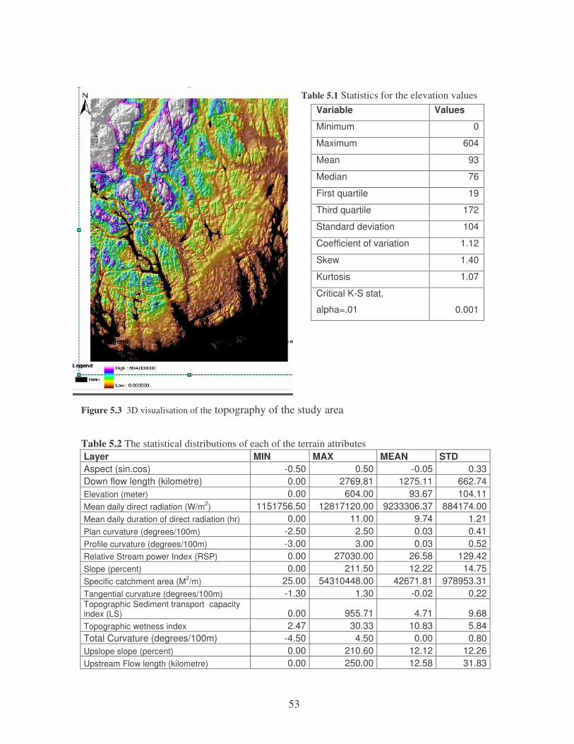
53
Table 5.1 Statistics for the elevation values
Figure 5.3 3D visualisation of the topography of the study area Table 5.2 The statistical distributions of each of the terrain attributes Layer MIN MAX MEAN STD Aspect (sin.cos) -0.50 0.50 -0.05 0.33 Down flow length (kilometre) 0.00 2769.81 1275.11 662.74 Elevation (meter) 0.00 604.00 93.67 104.11 Mean daily direct radiation (W/m2) 1151756.50 12817120.00 9233306.37 884174.00 Mean daily duration of direct radiation (hr) 0.00 11.00 9.74 1.21 Plan curvature (degrees/100m) -2.50 2.50 0.03 0.41 Profile curvature (degrees/100m) -3.00 3.00 0.03 0.52 Relative Stream power Index (RSP) 0.00 27030.00 26.58 129.42 Slope (percent) 0.00 211.50 12.22 14.75 Specific catchment area (M2/m) 25.00 54310448.00 42671.81 978953.31 Tangential curvature (degrees/100m) -1.30 1.30 -0.02 0.22 Topographic Sediment transport capacity index (LS) 0.00 955.71 4.71 9.68 Topographic wetness index 2.47 30.33 10.83 5.84 Total Curvature (degrees/100m) -4.50 4.50 0.00 0.80 Upslope slope (percent) 0.00 210.60 12.12 12.26 Upstream Flow length (kilometre) 0.00 250.00 12.58 31.83
Variable Values
Minimum 0
Maximum 604
Mean 93
Median 76
First quartile 19
Third quartile 172
Standard deviation 104
Coefficient of variation 1.12
Skew 1.40
Kurtosis 1.07
Critical K-S stat,
alpha=.01 0.001

54
5.1.3 Interrelationships among the Terrain Attributes
The Matrix of the Pearson’s correlation coefficient among the terrain attributes are presented
in table 5.3. The correlation coefficients vary from -0.99 to 0.83. Those greater than +0.4 or
less than -0.4 are presented in bold. As per the definition of correlation coefficients, when
two variables have positive correlation it indicates that increase in one variable is
accompanied by the increase in the other variable proportionate to the correlation coefficient;
where as, negative correlation between two variables indicate that increase in one variable is
accompanied by the decrease in the other variable proportionate to the correlation coefficient.
Besides, it shows that the presence of two highly correlated data in a dataset may not increase
the information content of the dataset.
The table shows that all the curvature parameters are strongly correlated negatively or
positively. The weakest correlation is observed between tangential and profile curvature
indicating the importance of them as indicators of curvature. Elevation, slope and downstream
flow length are positively correlated. This shows that elevated parts of the area are steeper in
slope and are obviously far from drainage outlets. The topographic wetness index is positively
correlated with the upstream flow length and negatively correlated with slope and the
topographic erosion index (LS). Topographic erosivity index and relative stream power index
have strong positive correlation creating doubt the use of both t the same time. Aspect and
specific catchment area are only very weakly related to any of the terrain attributes. For all
other correlations one has to look closely to table 5.3.

55
Table 5.3 Correlation Coefficients found among the terrain attributes
Layer Aspect
Total Curvature
Downstrream Flow length
Mean Daily Radiation Duration
Elevation
Topographic erosion index Slope
Plan curvature
Profile curvature
Upslope slope
Mean daily radiation
Stream power index
Specific catchment area
Tangential curvature
Upstream Flow length
Wetness Index
Aspect 1.00 Total Curvature -0.01 1.00 Downstream Flow length 0.17 0.00 1.00 Mean Daily Radiation Duration -0.19 0.35 -0.35 1.00 Elevation 0.14 0.06 0.62 -0.32 1.00 Topographic erosion index 0.11 -0.22 0.22 -0.51 0.27 1.00 Slope 0.18 0.38 0.29 -0.45 0.43 0.51 1.00 Plan curvature 0.01 0.83 0.00 0.21 0.05 -0.21 0.31 1.00 Profile curvature 0.02 -0.90 0.00 -0.37 -0.05 0.17 -0.35 -0.50 1.00 Upslope slope 0.16 0.01 0.23 -0.61 0.31 0.37 0.62 0.13 0.08 1.00 Mean daily radiation -0.07 0.04 -0.09 0.41 -0.08 -0.14 -0.17 0.01 -0.04 -0.16 1.00 Stream power index 0.04 -0.17 0.12 -0.23 0.13 0.77 0.15 -0.20 0.10 0.12 -0.05 1.00 Specific catchment area 0.00 -0.02 -0.01 0.01 -0.03 -0.01 -0.03 -0.01 0.02 0.01 0.01 0.00 1.00 Tangential curvature -0.01 -0.82 0.00 -0.21 -0.05 0.21 -0.31 -0.99 0.49 -0.12 -0.01 0.20 0.01 1.00 Upstream Flow length -0.10 -0.09 -0.25 0.17 -0.24 -0.08 -0.27 -0.09 0.06 -0.17 0.03 0.01 0.31 0.09 1.00 Wetness Index -0.24 0.09 -0.41 0.47 -0.44 -0.34 -0.53 0.05 -0.11 -0.35 0.11 -0.10 0.12 -0.05 0.58 1.00

56
5.2 Relationship between Terrain Attributes and Soil Properties
5.2.1 Correlation As stated in the methodology part, the fact that the sample sizes are limited for this analysis
does not encourage saying much about the relationships. However, having this fact on the
background, the following points can be pointed out about the relationship between terrain
attributes and some topsoil properties based on the result in table 5.4. Only those terrain
attributes with significant correlations are presented in the table here. The rest are found in
appendix 1.
• Clay and KHNO3- have high positive correlation with upstream flow length and
specific catchment area. They have negative correlation with slope and downstream
flow length. These indicate that areas which receive flow over long distance, from
large area are more likely to contain more clay and KHNO3- compared to their
opposites. Besides, the steeper the slope and the farther it is from the catchment outlet,
the lower are its clay and KHNO3- contents. Although not presented, there is also high
positive correlation between soils clay content and its content of KHNO3-.
• Extractible Nitrogen and Organic carbon positively correlated with topographic
wetness index and specific catchment area and negatively correlated with downstream
flow length. This means soils of the areas that receive flow from large areas, and
consequently have the tendency to get wet, have higher organic matter and nitrogen
content. On the other hand, as the place gets far away from drainage outlets, soil
organic matter content decreases. Besides, there is naturally high correlation between
soil organic carbon content and nitrogen content.
• No significant correlation was found between the terrain attributes and the soils pH
levels.

57
Table 5.4 Correlation Coefficients and their significance found between terrain attributes and some topsoil properties
Correlations
Terrain/Soil Attributes Clay Organic Carbon
Kjeldahl’s Nitrogen pHCaCl2 KHNO3
Pearson Correlation -.40(*) 0.08 -0.05 -0.27 -.41(*)
Sig. (2-tailed) 0.03 0.67 0.81 0.23 0.04
Slope
N 29.00 29.00 29.00 21.00 27.00 Pearson Correlation -.60(**) -.40(*) -.48(**) 0.32 -0.13
Sig. (2-tailed) 0.00 0.04 0.01 0.16 0.52
Downstream flow length
N 29.00 29.00 29.00 21.00 27.00 Pearson Correlation .41(*) 0.26 0.29 -0.17 .64(**)
Sig. (2-tailed) 0.03 0.17 0.13 0.47 0.00
Upstream flow length
N 29.00 29.00 29.00 21.00 27.00 Pearson Correlation -0.04 .40(*) 0.35 0.01 0.07
Sig. (2-tailed) 0.82 0.04 0.06 0.97 0.75
Topographic Wetness index
N 29.00 29.00 29.00 21.00 27.00 Pearson Correlation .52(**) .50(**) .61(**) 0.06 .44(*)
Sig. (2-tailed) 0.00 0.01 0.00 0.80 0.02
Specific catchment area
N 29.00 29.00 29.00 21.00 27.00
**. Correlation is significant at the 0.01 level (2-tailed). *. Correlation is significant at the 0.05 level (2-tailed).
5.2.2 Prediction of Soil Properties Using Multiple Linear Regression The results of multiple linear regression analysis show how much the collection of terrain
attributes contribute to the variation of a given soil property. It also enabled to construct a
linear regression model that can be used for the prediction of the values of the soil properties.
The results are presented and discussed only for clay content, Extractible (Kjeldahl’s)
nitrogen, and Potassium Nitrate (KHNO3-). The other soil attributes did not yield significant
regression. The results of the regression prediction of these three and their comparison with
kriging interpolation are presented case by case in the forthcoming text.
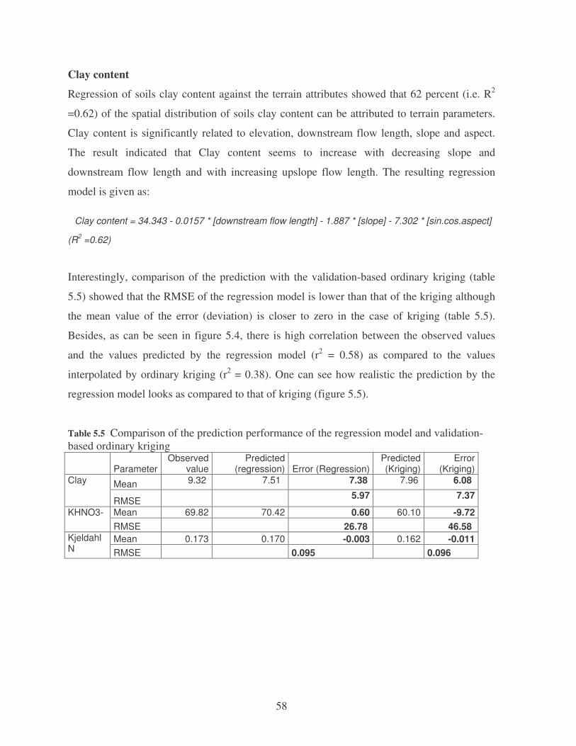
58
Clay content
Regression of soils clay content against the terrain attributes showed that 62 percent (i.e. R2
=0.62) of the spatial distribution of soils clay content can be attributed to terrain parameters.
Clay content is significantly related to elevation, downstream flow length, slope and aspect.
The result indicated that Clay content seems to increase with decreasing slope and
downstream flow length and with increasing upslope flow length. The resulting regression
model is given as:
(R2 =0.62)
Interestingly, comparison of the prediction with the validation-based ordinary kriging (table
5.5) showed that the RMSE of the regression model is lower than that of the kriging although
the mean value of the error (deviation) is closer to zero in the case of kriging (table 5.5).
Besides, as can be seen in figure 5.4, there is high correlation between the observed values
and the values predicted by the regression model (r2 = 0.58) as compared to the values
interpolated by ordinary kriging (r2 = 0.38). One can see how realistic the prediction by the
regression model looks as compared to that of kriging (figure 5.5).
Table 5.5 Comparison of the prediction performance of the regression model and validation-based ordinary kriging
Parameter Observed
value Predicted
(regression) Error (Regression) Predicted (Kriging)
Error (Kriging)
Mean 9.32 7.51 7.38 7.96 6.08 Clay
RMSE 5.97 7.37
Mean 69.82 70.42 0.60 60.10 -9.72 KHNO3- RMSE 26.78 46.58 Mean 0.173 0.170 -0.003 0.162 -0.011 Kjeldahl
N RMSE 0.095 0.096
Clay content = 34.343 - 0.0157 * [downstream flow length] - 1.887 * [slope] - 7.302 * [sin.cos.aspect]

59
0.00
5.00
10.00
15.00
20.00
25.00
30.00
35.00
0.00 5.00 10.00 15.00 20.00 25.00 30.00 35.00
Clay_meaured
Cla
y_re
gres
sed
Clay_regressed = 4.2 + 0.66*clay_meauredR2 = =0.58
1:1
0.00
5.00
10.00
15.00
20.00
25.00
30.00
35.00
0.00 5.00 10.00 15.00 20.00 25.00 30.00 35.00
Clay_measured
clay
_kri
ged
Clay_kriged = 6.45 + 0.5*clay_meauredR2 = =0.38 1:1
Figure 5.4 Regression predicted clay content versus observed (left) and Kriged versus observed (right)
Figure 5.5 Kriging interpolated clay content together with the data sample points (left) and regression predicted
clay map (right). The map covers only part of the study area where profile data were available.

60
0.00
50.00
100.00
150.00
200.00
0.00 50.00 100.00 150.00 200.00
KHNO3_measured
KH
NO
3_re
gres
sed
KHNO3_regressed = 28.67 + 0.6*KHNO3_meauredR2 = 0.60 1:1
0.00
50.00
100.00
150.00
200.00
0.00 50.00 100.00 150.00 200.00
KHNO3_measured
KH
NO
3_kr
iged
KHNO3_kriged = 52.38 + 0.11KHNO3_measuredR-square = 0.03 1:1
Potassium Nitrate (KHNO3-)
The correlation analysis between potassium nitrate and the terrain attributes showed that
negative correlation exists between soils KHNO3- content and slope and strong positive
correlation between KHNO3- and upslope flow length and the topographic wetness index. The
regression of KHNO3- against the terrain parameters showed the same relationship. It further
showed that 62% of the spatial variation of KHNO3- can be explained by the terrain attributes.
The resulting regression model is given as:
(R2 = 0.62)
Again as in the case of clay, the regression predicted value has much lower RMSE and an
error mean very close to zero as compared to ordinary kriging. The graphs in figure 5.6 show
that the correlation between the original data and the regression predicted values is much
higher (R2 = 0.60) compared to the kriging interpolated (R2 = 0.03), which indicates almost a
failure of the kriging interpolation.
Figure 5.6 Regression predicted versus observed (left) and Kriged versus observed (right) KHNO3- data
KHNO3- = 97.387 - 8.329 * [slope] + 1.6 * [mean upstream flow length] + 0.36 * [wetness index]

61
0.00
0.05
0.10
0.15
0.20
0.25
0.30
0.35
0.40
0.45
0.00 0.10 0.20 0.30 0.40
KjeldN_measured
Kje
ldN
_reg
ress
ed
KjeldN_regressed = 0.07 + 0.6*KjeldN_measuredR-square = 0.40 1:1
0.00
0.05
0.10
0.15
0.20
0.25
0.30
0.35
0.40
0.00 0.05 0.10 0.15 0.20 0.25 0.30 0.35 0.40
KjeldN_measured
Kje
ldah
lN_K
rige
d
KjeldN_kriged = 0.1 + 0.37*KjeldN_measuredR-square = 0.30 1:1
Extractible (Kjeldahl’s) Nitrogen
The result of the multiple linear regressions showed that nitrogen is related to elevation,
downstream flow length, the topographic wetness index, slope and aspect. It further indicated
that topographic attributes account for about 67 percent (R2 = 0.67) of the spatial variation of
soils extractible nitrogen content. The resulting regression model is given as:
(R2 = 0.67)
The regression prediction predicted the mean value better with error mean much closer to zero
and with a slightly lower RMSE compared to the kriging interpolation (table 5.5). The graphs
in figure 5.7 depict how much each predictive approach reproduced the original data. It also
confirms that the regression prediction performs better (R2 = 0.40) compared to the
interpolation by kriging (R2 = 0.31).
Figure 5.7 Regression predicted versus observed (left) and Kriged versus observed (right) N data
Kjeldahl_N = 0.361 - 0.000101 * [downstream. Flow length] + 0.002 * [wetness index] - 0.007 * [tangent curve] + 0.022 * [ LS] - 0.096 * [si.ncos.aspect] + 0.002 * [elevation] - 0.069 * [slope]

62
5.3 Digital Mapping of Soil Classes as Discrete Objects Using
Terrain Classification Algorithms
5.3.1 Analysis Of Variance Analysis of variance among the soil classes showed that there is significant variation among
the soil classes on all terrain attributes. The F-values of all the terrain attributes indicate that
the null hypothesis is rejected (table 5.6). Accordingly, there is significant difference between
the soil classes in all terrain attributes. Hoverer, pair-wise comparison between two soil
classes based on each terrain attribute, although not presented due to its length, showed
different picture. Some terrain attributes are capable of distinguishing some soil classes while
they are incapable of doing the same between some other soil classes. The result in general
showed that all the terrain attributes are important in distinguishing soil classes but not all
terrain attributes are important for all soil classes.
The ANOVA result shows that based on their significance and their capability to separate soil
classes (look at the F-values in table 5.6), the terrain attributes can be arranged as follows
from the most significant to the least significant: elevation, downstream flow length, mean
duration of daily direct radiation, slope, upslope slope, wetness index, and flow length,
Sediment Transport Index (LS), profile curvature, aspect, etc. The terrain attribute with the
least significance, i.e. with the smallest F value, was found to be plan curvature. This shows
that, first and foremost, the soil classes are spatially distributed based on elevation, then
distance from drainage outlet, followed by slope, etc.

63
Table 5.6 ANOVA result of the soil classes against the terrain attributes
5.3.2 Object-Oriented Supervised Terrain Classification Approach to
Digital Soil Mapping
There are three important analysis results of this approach that needs to be presented here:
First, the segmentation of homogeneous terrain attributes: Segmenting terrain-objects at
appropriate level was not found to be an easy task and required multiple try as it is solely
based on trial and error. The final result which gave maximum classification accuracy was
conducted at scale value of 20 using all the terrain attributes with shape factor of 0.1 shared
between smoothness and compactness equally. This segmented the 2933694 pixels
(1401columns by 2094 rows) into 327238 terrain objects, decreasing the units to be classified
by almost 90 percent.
Second, the features used for the classification: The identification of the best combination of
features was based on how well the features separated the soil classes. The separation
distance, which indicates how well classes are distinct, increased with the number of features
Attribute (factor) Sum of Squares
degrees of freedom Mean Square F Sig.
Elevation 11591085,83 13,00 891621,99 1461,54 0,00 Downstream Flow Length 217390769,21 13,00 16722366,86 284,71 0,00 Mean daily duration of direct radiation 2096,43 13,00 161,26 272,96 0,00 Slope 63300,18 13,00 4869,24 133,38 0,00 Upslope slope 86467,71 13,00 6651,36 86,14 0,00 Topographic wetness index 35097,87 13,00 2699,84 65,06 0,00 Topographic Sediment transport capacity index (LS) 11530,66 13,00 886,97 62,18 0,00 Profile curvature 33,84 13,00 2,60 34,66 0,00 Aspect(sin.cos) 52,07 13,00 4,01 33,23 0,00 Relative Stream power Index (RSP) 648995,39 13,00 49922,72 23,81 0,00 Total curvature 51,86 13,00 3,99 23,79 0,00 Mean daily direct radiation 667941478839501,00 13,00 51380113756884,70 16,05 0,00 Upstream Flow length 166149,49 13,00 12780,73 11,10 0,00 Specific catchment area 4124914809726,60 13,00 317301139209,74 8,17 0,00 Tangential curvature 0,85 13,00 0,07 5,10 0,00 Plan curvature 2,66 13,00 0,20 5,09 0,00

64
until the optimum number was reached, then it started to decrease (figure 5.8). The final
combination with relatively best result was obtained by inserting 47 features which were
optimized by the program to 21 features with best minimum separation distance of 1.7. These
features included the mean, standard deviation and mean difference to the scene mean of:
elevation, slope, downstream flow length, aspect, specific catchment area, upstream flow
length, and wetness index. The result still agrees with the result of the ANOVA presented
earlier in table 5.6 with minor differences.
Figure 5.8 Separation distance between sample soil classes as plotted against the number of features (dimension)
Third, the classification result and its accuracy: The classification result (figure 5.9) and its
accuracies, presented in table 5.7, were obtained after so many trials. It was learnt that the
approach seems to be working for the mapping of some soil types while it fails for others. In
the end, the overall accuracy could not go beyond 30 percent (table 5.7). Umbrisols,
Cambisols, Luvisols and Albeluvisols have relatively higher level of prediction accuracy, with
Umbrisols getting the highest accuracy. Where as, the other soils have very low prediction
accuracy indicating almost failure of the method. The accuracy decreased as the scale factor
increased or decreased from the optimum scale factor of 20.
The area coverage of the different soil classes in the whole study area is also presented in the
bar chart of figure 5.11. This helps to compare the area coverage of the soils in the reference
map with that in the prediction map. Besides, the accuracies were related to the area coverage.
Accordingly, both producer and user accuracies correlated with the area coverage of the soils
(table 5.8). The correlation is even stronger with the prediction map. This indicates that the
more widespread soils in the area have better accuracies as can actually be seen in table 5.6.
Besides, there is strong correlation between the soils area coverage in the reference map and

65
in the prediction map. This indicates that the method almost kept the area proportion of the
soil classes during the prediction. There is good correlation between the user and producer
accuracies indicating comparable errors of omission and commission.
Table 5.7 Accuracy of the Object-oriented classification Class Producer accuracy User accuracy Umbrisol 76.09 44.33 Luvisol 31.82 12.97 Cambisol 31.69 31.95 Albeluvisol 14.26 28.64 Anthropic Regosol 1.64 4.31 Podzol 1.53 4.71 Histosol 0.97 8.28 Leptosol 0.94 0.91 Phaeozem 0.57 4.68 Gleysol 0.52 6.99 Anthrosol 0.50 0.46 Arenosol 0.49 3.81 Fluvisol 0.33 3.48 Regosol 0.00 0.00 Overall Accuracy 30.90
Table 5.8 Relationship of the prediction accuracies to other parameters
correlation statistics Observed area cover
predicted area cover
producer accuracy
User accuracy
Observed area cover 1 predicted area cover 0.78 1 producer accuracy 0.37 0.57 1 User accuracy 0.36 0.46 0.88 1

66
Figure 5.9 Map of the soil classes as predicted by object-oriented terrain classification

67
5.3.3 Pixel-Based Supervised Terrain Classification Approach to Digital
Soil Mapping
The result of the ordinary pixel-based supervised classification is presented in figure 5.10.
The figure shows the spatial distribution of each soil type as predicted by supervised
classification of terrain pixels. The accuracies of the prediction are also presented in table
5.9. The overall accuracy could not go beyond 14 percent. That is by far very low in absolute
sense and compared to the result of the object-oriented classification. Again, the same soil
classes tend to have higher user accuracy as in the case of object-oriented classification.
However, the producer accuracy has different trend. There seems to be very low correlation
between producer and user accuracy. There is also loose connection between the area cover of
a soil type and its accuracy of prediction. The prediction map shows that Podzols (36%) are
the most wide-spread soil type followed by Umbrisols (20%). This is contrary to the original
soil map and to the object-oriented prediction.
Table 5.9 Pixel-based prediction accuracies Class Producer accuracy User Accuracy Podzol 39.16 4.58 Umbrisol 31.26 34.76 Regosol 29.73 0.69 Arenosol 22.98 4.06 Cambisol 14.47 41.56 Fluvisol 4.18 6.18 Histosol 3.74 5.29 Gleysol 2.25 9.38 Luvisol 2.15 20.24 Anthropic Regosol 2.15 4.33 Phaeozem 2.11 1.94 Anthrosol 0.38 1.65 Leptosol 0.16 1.31 Albeluvisol 0.06 20.53 Overall Accuracy 13.58

68
Figure 5.10 Map of the soil classes as predicted by pixel-based supervised classification

69
5.4 Digital Mapping of Soil Classes as Fuzzy Variables
5.4.1 Multinomial Logistic Regression The overall multinomial logistic model was found to be significantly fit at p<0.05. Table 5.10
further shows that the most significant terrain attributes in influencing the spatial distribution
of the soil classes were found to be elevation, downstream flow length, mean daily duration of
radiation, mean upslope slope, slope aspect, etc (See appendix 2 for the raw result of the
analysis). In fact, with the exception of plan curvature all of them were found to be
significantly influential.
On the other hand, almost all soil classes were found to be influenced by at least two terrain
attributes. The extent of the influence is presented in table 5.11. The magnitudes in the table
indicate the factor by which the odds ratios of the soil classes change if the value of a given
terrain attribute is increased by a unit. Besides, values greater than 1 indicate that increase in
the values of the terrain attribute results in the increase in the odds ratios of that soil class,
although the magnitude has no direct meaning for the values of the probabilities. On the other
hand, values less than 1 show the opposite of this. The further the values are from 1, the
stronger the change in the odds ratios that is caused by increase in one unit of the predictor.
This will be discussed in detail later as it needs cautionary explanation. The terrain attributes
which were found significantly influential in the spatial distribution of each soil class and the
type and extent of the influences are presented in table 5.10.
Table 5.10 The significance of each terrain attribute in the overall model Likelihood Ratio Tests
Model fitting criteria Likelihood Ratio Tests
Effect -2 Log Likelihood of Reduced Model Chi-Square
degree of freedom Sig.
Elevation 223469.33 18769.14 13.00 0.00 Downstream flow length 215214.89 10514.70 13.00 0.00 Mean daily duration of radiation 206495.91 1795.72 13.00 0.00 Mean upslope slope 205509.50 809.32 13.00 0.00 slope 205030.49 330.30 13.00 0.00 Aspect (sin.cos) 204857.72 157.53 13.00 0.00

70
Received Mean daily direct radiation 204836.65 136.46 13.00 0.00 Upstream flow length 204802.35 102.16 13.00 0.00 Specific catchment area 204786.02 85.83 13.00 0.00 Wetness Index 204773.80 73.61 13.00 0.00 Erosion Index (LS) 204754.32 54.13 13.00 0.00 Relative Stream Power Index 204754.30 54.11 13.00 0.00 Tangent Curvature 204732.28 32.10 13.00 0.00 Total Curveture 204729.45 29.26 13.00 0.01 Profile curvature 204725.98 25.79 13.00 0.02 Plan Curvature 204 667.44 16.54 13.00 0.22 Table 5.11 The influence of each terrain attribute on each soil class as expressed in odd ratios Parameter Estimates Predictor EXP(B) of Soil class
AB AR AT CM FL GL HS LP LV PH PZ RG Rgah
Aspect (sin.cos) 1.39 0.27 1.35 1.17 0.48 1.90 Total Curvature 0.13 Downstream Flow Length 1.01 1.01 1.01 1.01 1.01 1.01 1.01 0.99 1.01 0.99 0.99 1.01 0.99 Elevation 0.99 0.91 0.98 0.95 0.98 0.99 1.01 1.05 0.98 1.02 1.00 1.01 0.97 Topographic erosion index (LS) 1.12 1.12 slope 0.93 1.05 0.86 0.86 0.85 0.92 0.85 Profile curvature 0.10 Mean Upslope slope 0.99 0.96 0.96 0.99 1.02 0.97 0.99 Relative stream power index 1.00 0.99 0.99 Specific catchment area 0.99 0.99 0.99 0.99 0.99 Tangential curvature 0.03 Upstream flow length 1.01 1.01 1.00 1.01 1.01 Wetness index 0.99 0.95 0.98 1.04 0.96 Mean duration of direct radiation 0.72 3.21 0.62 0.37 0.81 0.59 0.50 0.75 1.74 0.70 Mean direct shortwave radiation 1.00 1.00 1.00 1.00 1.00 1.00 1.00 1.00 a. The reference category is: UM
The other outcome of the analysis is the possibility of constructing logit models for each soil
class except for the reference soil class. Each model enables to predict the probability that a
given soil class exists in a given area given the values of the terrain attributes which are found
to be significantly influential in the spatial distribution of that soil class. More correctly, the
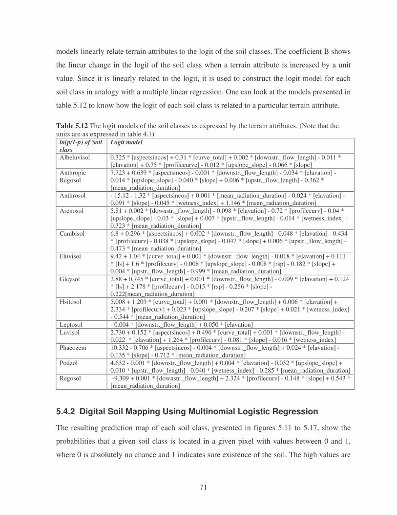
71
models linearly relate terrain attributes to the logit of the soil classes. The coefficient B shows
the linear change in the logit of the soil class when a terrain attribute is increased by a unit
value. Since it is linearly related to the logit, it is used to construct the logit model for each
soil class in analogy with a multiple linear regression. One can look at the models presented in
table 5.12 to know how the logit of each soil class is related to a particular terrain attribute.
Table 5.12 The logit models of the soil classes as expressed by the terrain attributes. (Note that the units are as expressed in table 4.1)
ln(p/1-p) of Soil class
Logit model
Albeluvisol 0.325 * [aspectsincos] + 0.31 * [curve_total] + 0.002 * [downstr._flow_length] - 0.011 * [elavation] + 0.75 * [profilecurve] - 0.012 * [upslope_slope] - 0.066 * [slope]
Anthropic Regosol
7.723 + 0.639 * [aspectsincos] - 0.001 * [downstr._flow_length] - 0.034 * [elavation] - 0.014 * [upslope_slope] - 0.040 * [slope] + 0.006 * [upstr._flow_length] - 0.362 * [mean_radiation_duration]
Anthrosol - 15.12 - 1.32 * [aspectsincos] + 0.001 * [mean_radiation_duration] - 0.024 * [elavation] - 0.091 * [slope] - 0.045 * [wetness_index] + 1.146 * [mean_radiation_duration]
Arenosol 5.81 + 0.002 * [downstr._flow_length] - 0.098 * [elavation] - 0.72 * [profilecurv] - 0.04 * [upslope_slope] - 0.03 * [slope] + 0.007 * [upstr._flow_length] - 0.014 * [wetness_index] - 0.323 * [mean_radiation_duration]
Cambisol 6.8 + 0.296 * [aspectsincos] + 0.002 * [downstr._flow_length] - 0.048 * [elavation] - 0.434 * [profilecurv] - 0.038 * [upslope_slope] - 0.047 * [slope] + 0.006 * [upstr._flow_length] - 0.473 * [mean_radiation_duration]
Fluvisol 9.42 + 1.04 * [curve_total] + 0.001 * [downstr._flow_length] - 0.018 * [elavation] + 0.111 * [ls] + 1.6 * [profilecurv] - 0.008 * [upslope_slope] - 0.008 * [rsp] - 0.182 * [slope] + 0.004 * [upstr._flow_length] - 0.999 * [mean_radiation_duration]
Gleysol 2.88 + 0.745 * [curve_total] + 0.001 * [downstr._flow_length] - 0.009 * [elavation] + 0.124 * [ls] + 2.178 * [profilecurv] - 0.015 * [rsp] - 0.256 * [slope] - 0.222[mean_radiation_duration]
Hsitosol 5.008 + 1.209 * [curve_total] + 0.001 * [downstr._flow_length] + 0.006 * [elavation] + 2.334 * [profilecurv] + 0.023 * [upslope_slope] - 0.207 * [slope] + 0.021 * [wetness_index] - 0.544 * [mean_radiation_duration]
Leptosol - 0.004 * [downstr._flow_length] + 0.050 * [elavation] Luvisol 2.730 + 0.152 * [aspectsincos] + 0.496 * [curve_total] + 0.001 * [downstr._flow_length] -
0.022 * [elavation] + 1.264 * [profilecurv] - 0.081 * [slope] - 0.016 * [wetness_index] Phaeozem 10.332 - 0.706 * [aspectsincos] - 0.004 * [downstr._flow_length] + 0.024 * [elavation] -
0.135 * [slope] - 0.712 * [mean_radiation_duration] Podzol 4.632 - 0.001 * [downstr._flow_length] + 0.004 * [elavation] - 0.032 * [upslope_slope] +
0.010 * [upstr._flow_length] - 0.040 * [wetness_index] - 0.285 * [mean_radiation_duration] Regosol -9.309 + 0.001 * [downstr._flow_length] + 2.324 * [profilecurv] - 0.148 * [slope] + 0.543 *
[mean_radiation_duration]
5.4.2 Digital Soil Mapping Using Multinomial Logistic Regression
The resulting prediction map of each soil class, presented in figures 5.11 to 5.17, show the
probabilities that a given soil class is located in a given pixel with values between 0 and 1,
where 0 is absolutely no chance and 1 indicates sure existence of the soil. The high values are

72
shown in red in all of the maps. With the exception of Anthrosols and Regosols the maximum
probability values of all the other soil classes were above 0.5. The maps were found to be very
reliable when evaluated using the two approaches explained in the methodology part of this
thesis. When the maps were evaluated based on the generic definition of the soil classes and
comparison with the (Solbakken et al., 2006) high probability areas for a soil class more or
less coincided with areas covered with that soil class.
Besides, the probability maps were investigated through 3D visualization and correlations
studies with other terrain attributes. These five groups listed below fit well with the theory of
the spatial distribution of soil classes and correlated visually well with the empirical soil map.
1. Soils with high probability on the hills and mountains and steep areas: These are
Leptosols dowelling the hill tops and Umbrisols and Podzols dowelling steep areas.
2. Soils with high probabilities in the valleys and very gentle slopes: these are cambisols,
Fluvisols, Luvisols, and Albeluvisols.
3. Soils with high probabilities at the depressions and beach playas: These are Gleysols
and Arenosols
4. Soils that that have high probabilities in valleys: these are Histosols and luvisols
5. Soils with unreliable topographic relations: Anthrosols, regosols and anthropic
regosols.
Probability correlation: The basic guideline here was that soils that are known to develop in
similar environment are expected to have higher positive correlation in their probabilities
while those develop under opposite environment are expected to have higher negative
correlation.
The result, which further strengthened the reliability of the probability mapping, is presented
in table 5.13. Very high correlation values are presented in bold. Based on the result, some
groups which have high positive correlation among themselves could be identified:
1. Histosol, Fluvisol and Gleysol group: The FAO definition and characterization of the
environment of this group shows some common feature. The first two develop in areas
where there is accumulation of organic matter which requires the presence of wetness.

73
The presence of wetness links these two to Gleysol as Gleysols are created due to poor
drainage.
2. Luvisol, Albeluvisol, Cambisol and Regosol group: These soils have common
features. These soil classes are known to dwell flat and gently sloping areas with
pedogenically favorable conditions.
3. The third group comprises of Podzol and Umbrisol which have very high positive
correlation. These two soil classes are found basically under the same physical
environment that is subjected to bleaching and eluviation, but they differ in that the
second contains high organic matter.
4. Anthrosol and Anthropic regosol correlated well indicating the spatial correlation of
human activities that lead to the formation of these soil classes.
5. Leptosol correlates poorly or negatively with all of the soil classes as it dwells
topographically well distinguished environment, the hilltops.
6. Phaeozem also correlated poorly with any soil class indicating that it too occupied a
unique environment in this study area.
Table 5.13 Correlation among the probabilities of the soil classes Layer AB AR AT CM FL GL HS LP LV PH PZ RG Rgah UM AB 1.00 AR -0.38 1.00 AT -0.24 0.54 1.00 CM 0.05 0.52 0.13 1.00 FL 0.12 -0.07 -0.12 0.23 1.00 GL 0.26 0.06 0.22 0.22 0.33 1.00 HS 0.31 -0.28 -0.21 -0.19 0.30 0.44 1.00 LP -0.35 -0.40 -0.35 -0.57 -0.25 -0.46 -0.14 1.00 LV 0.39 0.16 0.36 0.45 0.19 0.57 0.01 -0.71 1.00 PH -0.20 -0.12 0.05 -0.24 -0.03 -0.06 -0.01 -0.03 -0.17 1.00 PZ 0.13 -0.35 -0.23 -0.26 -0.06 -0.30 -0.08 -0.06 -0.17 0.00 1.00 RG 0.41 -0.18 0.07 -0.13 0.06 0.52 0.40 -0.23 0.36 -0.04 -0.04 1.00 Rgah -0.41 0.52 0.53 0.17 -0.07 -0.02 -0.29 -0.43 0.15 0.16 -0.14 -0.17 1.00 UM 0.30 -0.37 -0.24 -0.23 -0.08 -0.26 -0.03 -0.08 -0.08 -0.10 0.80 0.00 -0.26 1.00

74
Figure 5.11 Probability Distribution of Albeluvisol (left) and Arenosol (right)
Figure 5.12 Probability Distribution of Anthrosol (left) and Cambisol (right)

75
Figure 5.13 Probability Distribution of Fluvisol (left) and Gleysol (right)
Figure 5.14 Probability Distribution of Histosol (left) and Leptosol (right)

76
Figure 5.15 Probability Distribution of Luvisol (left) and Phaeozem (right)
Figure 5.16 Probability Distribution of Regosol (left) and Podzol (right)

77
Figure 5.17 Probability Distribution of Anthropic Regosol (left) and Umbrisol (right)

78
6 DISCUSSION
6.1 Reflections on the Results
6.1.1 Digital Terrain Analysis Before proceeding to any discussion with other results, it is noteworthy to briefly discuss
digital representation of the terrain, the major uncertainties identified and the remedial
procedures applied. As presented in the result, statistics of terrain attributes, hypsometry, the
correlation matrix of the terrain attributes, and last but not least, 3D visualization were used to
present the characteristics of the topography digitally. They were all used because they
present different feature of the topography.
As can be seen from the statistics of the terrain attributes and the hypsometric curve and its
integral, the area is dominated by low altitude, gently slopped terrain. Hypsometry is
generally used as a measure of geomorphic development. Concave hypsometric curves as in
the case of this study indicate peneplained, i.e. geomorphologically and tectonically more
stabilized, landscapes (Hurtrez et al., 1999). Besides, hypsometric integral increases with
tectonic activities such as uplifting and is highly sensitive to land surface processes such as
erosion and deposition. The geology of the study area also shows that there is no dramatically
active tectonic and geomorphological processes taking place since the last ice age (Solbakken
et al., 2006; Sorensen, 1988). Therefore, it makes sense that, although there are relatively
slow geomorphological processes such as erosion and deposition in the area, the landscape
seems tectonically stabilized.
When one looks at the list of the terrain attributes analyzed, one might wonder if each of these
contains unique information. The correlation matrix tried to resolve this puzzle. As presented
in the result, some terrain attributes are highly correlated. There are many causes for these:
first, some terrain attributes correlate because they are simply different ways of expressing the
same parameter. E.g. the high positive correlation between the topographic erosion index (LS)
and the topographic stream power index alarms the reevaluation of the need for the use of
both of them. They seem to be redundancy of the same index as their values correlate and

79
they are both related to erosion. Second, some terrain attributes correlated due to their
inherent mathematical definition which explains the natural relationship between the
parameters. For example, the positive correlation between plan curvature and tangential
curvature is just due to their definition that tangential curvature is a product of plan curvature
and the sine of the slope (Gallant and Wilson, 2000). Third, some terrain attributes correlate
because they fulfill the natural logic of increasing one may result in the decrease or increase
of the other. The strong correlation between upslope flow length and specific catchment area
is obviously due to the fact that when flow comes from a very long distance it is likely that
large areas contribute to such flows increasing flow accumulation and contributing area per
pixel. Besides, one can also notice the obviously justifiable negative correlations of the
topographic wetness index with attributes such as elevation, slope and downstream flow
length and its positive correlation with upslope flow length. Fourth, some correlations
between the terrain attributes are just unique to the study area and do not show any
repeatability in another landscapes. These are important in expressing the nature of the
landscape. For instance, the correlation between elevation and slope in this area is just due to
the nature of the landscape such that high elevation areas are more rugged than low elevation
areas. The opposite would have been true had the area been dominated by table plateaus.
All those information discussed so far might tempt one to believe that digital terrain modeling
is without flaws. However, as the saying goes, the devil is in detail. One has to be aware of
the different sources of uncertainty. The errors that accompany the original DEM, the errors
that are introduced through DEM improvement processes, the errors that are introduced due to
the algorithms used to derive each terrain attributes, etc are all there to have impact.
The unrealistic high frequencies of elevation values at multiples of 20m, the interval of the
source contour, are just indicators of the poor performance of the interpolation algorithm used
to derive the DEM from the original data (Wilson and Gallant, 2000a). These repetitive high
frequencies were observed to be more pronounced in flat areas because, in flat areas, the
contours are spatially very scattered and the interpolated values during DEM creation
naturally tend to be pulled together around the values of the contour. The poor performance of
the aspect calculation algorithm that looks to limited search directions has also been depicted

80
in the histogram of the aspect where unrealistic high frequencies were observed at multiples
of 45 degrees (Wilson and Gallant, 2000a).
Artificial depressions are errors introduced due to a number of reasons such as data errors,
interpolation, and the limitations by horizontal and vertical resolutions that are unable to
incorporate the reality of ridges and streamlines (Creed-I.F and Lindsay-J.B, 2005). Their
removal is necessary for subsequent analyses in hydro-geomorphic applications (Creed-I.F
and Lindsay-J.B, 2005; Wilson et al., 2000). The removal of depression is actually helpful in
routing flows so that attributes such as flow direction, flow length, contributing area, etc are
realistically estimated. One has to be aware of the fact that the remedial measures are not only
solutions but they also introduce other sources of uncertainties. To remove depressions,
natural and artificial ones have to be differentiated first. But as admitted by (Wang and Liu,
2006) this is a tedious and complicated process that at the end may not even have great
advantages over simply removing entire depression.
The measures used in this thesis to remove artificial depressions (Darboux and Planchon,
2002; Planchon, 2001) involves enforced flow on flat areas in addition to the removal of
depression and spikes. The consequences of such depression removal procedures are variable
and deserve separate study. A study conducted by (Creed-I.F and Lindsay-J.B, 2005) revealed
that such procedures alter spatial and statistical distribution of terrain attributes. They state
that the degree to which each terrain attribute is affected is controlled by the number of
neighbors used in the processing of the terrain attribute. Removal of depressions and spikes
and the enforcement of flow on flat areas can create other artificial features in flat areas.
In any case, in this study it was observed that without the removal of depressions and spikes
and without enforced flow on flat areas, flow related terrain attributes and compound
attributes such as wetness index could not have been realistically estimated. Other than the
blockage of flows in depressed areas, spikes create unrealistically very high slopes which
have adverse effects on the estimation of other terrain attributes. Besides, flat areas will have
absolutely zero values of slope and undefined flow direction creating difficulty when

81
parameters which involve division by these attributes are estimated. Therefore, the remedial
procedures had enormous advantages.
6.1.2 Digital Terrain Analysis and Soil Properties The interpretation of the results of the relationship between the terrain attributes and the
topsoil properties needs caution due to a number of reasons. First, the sample size was not
large enough to enable to say much about the correlation with confidence. Second, the
samples were not collected with the intention of such analysis, and therefore their spatial
distribution was not taken into consideration. However, soil properties, although not exactly
the ones attempted in this study, have been predicted from terrain attributes by many
researchers (Bell et al., 2000; Chamran et al., 2002; Florinsky et al., 2002; McBratney et al.,
1995) with highly reliable results. Having these facts on the background, it is worthwhile to
comment on the correlations observed in this research.
The correlations of clay content with some terrain attributes in table 5.4 are very well in
agreement with theory of soil particle redistribution and erosion-deposition process (Brady
and Weil, 2002). The attributes influence soils clay content through their influence on the
movement of water and particles. KHNO3- also follows the pattern of clay as there is high
correlation between clay content and KHNO3- content. Therefore, it is no surprise that most of
the correlation and regression behavior of KHNO3- is related to that of clay.
The prediction of clay and KHNO3- is more reliable compared to that of the extractible
nitrogen. Clay and KHNO3- are highly related to parent material, topography and pedogenic
processes. Where as nitrogen is more related to climate, vegetation, and other properties such
as clay content, organic matter content, etc. It is even temporally very dynamic depending on
the local land use and season. Therefore, the role of topography is less pronounced or less
stable in such properties as nitrogen content compared to the other two. This fact has been
evidenced in the bivariate correlation matrix as well. Besides, nitrogen is highly related to the
organic carbon content of soils with which the terrain attributes of this area had very weak
correlation. The weak correlation with organic carbon content can be linked to the fact that it
is more of the presence of organic materials that dictate soils content of organic carbon than

82
the topography. The lack of correlation with pH can be ascribed to the fact that soils pH is
highly influenced by climate and parent material than topography. Therefore, significant
variation of pH at toposcale might not be encountered, in addition to the limitations of the
sample size.
Nonetheless, the prediction of the soil properties through multiple regression using terrain
attributes have shown its superiority to the most commonly used interpolation technique, i.e.
ordinary kriging. Kriging estimates variable values at unknown places based on the values of
the surrounding points and the distance between the unknown point and the points
surrounding it (Bishop and McBratney, 2001; Goovaerts, 1999), regardless of the local terrain
and other characteristics. It is solely based on distance and relies on the concept that ‘near
things are more alike than distance things’ of Tobler (Sui, 2004). On the other hand, the
regression prediction estimated the unknown values based on the local terrain characteristics
and using the relationship between terrain attributes and the soil property in question. Of
course, the values at the known points influence the setting up of the relationship, i.e. model
building. In reality two very close points can have very different values in a given soil
property (.e.g. clay content) due to abrupt changes in local terrain characteristics. Where
kriging considers such pixels as near pixels and relates their values, regression considers their
local slope, aspect, curvature or any other relevant terrain attribute to estimate their values.
That is why regression-prediction appears more realistic on the map (e.g. figure 5.5) and its
errors are lower (table 5.5).
One drawback that was observed from the results of the prediction of the soil properties is that
they fail in very steep and high altitude areas. This is simply due to the fact that the samples
used for the regression model building did not contain representatives of such areas.
Therefore, that led to a kind of model extrapolation, i.e. model use out of its domain area. It
would have been best to include samples from all types of landscape and/or stratify the area
so that different models are built for different strata. Regionalization is stressed by Florinsky
et al, (2002) in their attempt to predict soil properties using terrain attributes. Their studies
revealed that the relationship between soil properties and terrain attributes is dependent upon
spatial and temporal scale and depth of the soil where the soil properties are measured. Such

83
dependences have not been explored in this study simply because it was not the goal of the
research. However, one should be reminded of those facts.
6.1.3 Digital Terrain Analysis and Soil Classes One of the two conceptually different approaches to digital soil mapping followed in this
thesis was crisp (discrete) classification, the other being continuous (fuzzy logic) approach.
Before progressing to the spatial prediction of soils using crisp approach, analysis of variance
was conducted. This step was crucial because: first, it confirmed the theory that soil classes
are different in the type of terrain attribute they develop on; Second, it helped to figure out
which terrain attributes are more important in distinguishing soil classes. Without having
empirical evidence that the dependent attribute is really dependent on the predictor variables,
there would not have been any need of attempting the prediction.
When one looks at the list in the ANOVA result of table 5.6, it becomes clear that the
attributes are so arranged due to their direct or indirect roles in pedogenic processes. Those on
the top of the list (i.e. elevation, flow length, mean duration of daily radiation, wetness index,
slope, aspect, etc) are known to dictate the spatial distribution of temperature, radiation,
moisture and solid materials (Hugget and Cheesman, 2002; Wilson and Gallant, 2000a).
These are crucial factors of soil formation processes (Schaetzl and Anderson, 2005).
Therefore, the ANOVA result complies with the theory of pedogenesis.
ANOVA tests whether the mean values of each terrain attribute is significantly different from
one soil class to the other (Anderson, 2001) . Crisp (discriminant) classification is based on
the same idea (McCloy, 2006). It first defines means of each variable (e.g. terrain attribute)
for each class (e.g. soil class) based on the samples and includes the unknown pixels or
objects based on their proximity to the mean centers.
The two discriminant classification approaches used in this thesis, i.e. object-oriented and
pixel-based, are similar in concept but employ different procedures. The better performance
of the Object-oriented approach can be ascribed to the following reasons. First and foremost,
the approach classifies objects (adjacent pixels of similar terrain characteristics) rather than
individual pixels. Terrain objects are thus adjacent pixels which are not significantly different

84
in their values of the terrain attributes at that scale. It is a long established concept that the
boundaries of soil units tend to follow that of topographic units (Park et al., 2001; Thompson
et al., 2006). It is based on that concept that the famous soil-landscape model was developed
and has long been used in qualitative soil mapping. Therefore, classification of terrain objects
means classification of soil mapping units into soil classes. Pixels do not complement with
such concept.
Secondly, object-oriented approach provides extra features that are only related to objects or
classes that can be used in discriminating classes. These features can be the shape of the
objects of a given class, contextual features such as neighborhood, and geometry. Such
features are impossible to utilize in pixel-based classification as all pixels have the same
shape and geometry. The most important of these object and class related features in the case
of soil mapping has been found to be topological information such as relative distance to
neighboring class. This is because as explained in soil catena concept (Schaetzl and Anderson,
2005), soil classes tend to have a certain pattern of spatial distribution. Some soil classes tend
to be accompanied with a certain soil class.
Thirdly, Object-oriented approach in eCgnition offers the possibility of navigating through
different scales of object aggregation until the most appropriate level with high classification
accuracy is obtained. This helps to arrive at the aggregation level which best coincides with
the spatial extent of soil units. On the other hand, the only scale parameter in pixel-based
approach is the pixel resolution, which is fixed level of generalization. It has not come with a
surprise that the object-oriented approach performed better because of the aforementioned
reasons and other empirical researches conducted on other geographical objects such as land
cover (Mas et al., 2006; Whiteside and Ahmad, 2005) that comply with the findings of this
thesis.
In this research, regarding the segmentation (terrain object delineation) it has been learnt that
increasing the scale value to more than 50 showed that some soil units completely disappear
because their spatial extent is less than the object size. In such cases, collecting sample objects
for each class would be difficult, if not impossible, because objects that coincide with a single

85
class become hard to pass by. It was also learnt that increasing the shape parameter during
segmentation results in more geometrically similar terrain objects, which do not seem to be
natural, and leads to decreased classification accuracy. Although it needs further research, it
seems that DEMs with high spatial resolution are needed to navigate further between the scale
values without facing difficulty in identifying sample objects.
The classification algorithm used in eCgnition is the Nearest Neighbor Classifier. In
eCgnition this approach is used based on fuzzification and defuzzification concepts (Baatz et
al., 2000). (Baatz et al., 2000) First multidimensional fuzzy membership values are assigned
to the object for all classes based on its distance from the mean center of sample objects in the
multidimensional feature space, i.e. fuzzification. Then the object is assigned to the class for
which it has the highest membership value (the nearest neighbor), i.e. defuzzification. This
approach is different from the maximum likelihood classifier approach used in the pixel-based
classification where pixels are assigned membership values of either 0 (not belong to the
class) or 1 (belong to the class). This might also have consequences in the classification
accuracy and deserves separate research.
There were very high discrepancies among the accuracies of the soil classes. This applies to
both the object-oriented and pixel-based approaches. This was expected right from the
beginning and has a number of causative reasons:
• First, the spatial distributions of all soil types are not influenced by topography to the
same extent. Some soil classes are highly dictated by topography; where as, others are
dictated less by topography and more by parent material or climate or organisms.
Therefore, even if all the data, methodology and other things were perfect, variation in
accuracy among the soil classes can be expected.
• Second, the area coverage of the soil classes in the study area varies greatly. This
increases the chances of being accurate for the most abundant and decreases that of the
least abundant.
• Third, the sizes of soil units for the soil classes also vary greatly. Some soil classes,
especially those in the topographically more uniform areas, have large soil units; while,
those found on the topographically more rugged areas have small soil units. The larger the

86
soil unit, the better is the chance to coincide with terrain objects. It is even difficult to
collect sample objects for the small soil units because they may not totally cover a terrain
object at some scales, and they are divided into different kinds of terrain objects at smaller
scale values.
• Fourth, the number and the spatial distribution of the sample objects is one of the crucial
reasons why the accuracies vary a lot. Attempt was made to keep the number of the
sample objects in proportion with the area share of the soil classes. That could reduce the
statistical strengths of the least abundant soil classes. Besides, the spatial distribution of
the samples is the most difficult one to deal with. Attempt was made to evenly distribute
them across the entire area. However, even distribution does not guarantee the
representation of the various terrain types. Even the reference soil map from which the
samples were collected did not cover high elevation and steep slope areas. One would
therefore expect the bias of the samples and thence of the accuracies.
• Fifth, it is known that all those predictions were based on the terrain attributes which
were directly or indirectly derived from the elevation data (DEM). The DEM contains
uncertainties that are most likely to vary from steep areas to flat areas depending on the
source of the original data and the procedures applied on them. If the uncertainty varies
with terrain type, it means it varies with soil type. Therefore, the terrain attributes of the
soil classes which developed in the areas of high DEM uncertainty have not been well
represented or measured, leading to decreased prediction accuracy for such soil classes.
The logistic regression analysis employed in this research came up with a number of useful
results. First, it showed which terrain attributes are generally influential in the spatial
distribution of soils. The reason as to why some terrain attributes are very influential has been
discussed earlier and is related to their influence in the spatial distribution of radiation,
temperature and moisture. The only insignificant attribute is the plan curvature, which is the
curvature of aspect. This attribute also had the lowest F value in the analysis of variance. The
influence of the curvature of aspect is more represented by tangential curvature which
measures aspect curvature and combines that with the local slope (Gallant and Wilson, 2000).

87
Second, the result enabled to identify which terrain attributes influence the continuous spatial
variation of each soil class and to what degree. The extent of the influence is measured
through the odds ratios, i.e. EXP(B), of the terrain attributes for each soil class. One has to be
cautious in comparing the EXP(B) of one terrain attribute to the other because they are simply
not on the same scale. Notice that some terrain attributes have odds ratios, i.e. EXP(B), far
away from 1 (e.g. aspect, curvature) while others have either 1 or close to it (e.g. elevation,
flow length, etc) for most soil classes. Such differences are created due to two possible
reasons: First, due to the fact that one terrain attribute actually has greater or less effect on the
soil class than the other. Second, the unit value of one terrain attribute is practically of larger
order than that of the other. For example, a unit of elevation is a meter which does not
dramatically change the probability of any soil class. Where as, a unit of aspect, in this case
expressed as the product of the sine and cosine of the aspect in degrees, is a unitless 1 which
is of course very big because the entire 360 degrees is distributed from -1 to 1. Therefore, one
has to be reminded of the unit values when looking at the odds ratios of each terrain attribute.
This was the reason why terrain attributes with small measurement units were converted to a
unit that can reduce the magnitude. For example, the unit of flow length was converted from
meter to kilometer to cope with this situation, because a one unit change in the predictor has
to be meaningful (Peng et al., 2002). However, what is more important is whether the odds
ratio is greater than 1 which corresponds to the positive correlation of the linear regression, or
less than 1 which corresponds to the negative correlation of the linear regression.
Third, it helped to construct prediction models which enabled to predict the spatial
distribution of the probability of finding each soil type in the study area. Accordingly some
soil classes were found to have high probability values in the area while others have very low
due to a number of possible reasons. First, based on the sample data used for the model
construction, it has been found out that the terrain is more suitable for the development of
some soil classes, while it is less so for others. This applies to the very low maximum
probability values predicted for the almost non-present soil class in the study area, i.e.
Regosol. Second, the results of multinomial logistic regression is known to be biased by the
proportion of the samples, although not as strongly as its comparatives such as linear
regression (Peng et al., 2002; Raimundo et al., 2006 ). Since the proportion of the samples in

88
this research was not even, it may have had impact on the result. Third, the spatial distribution
of some soil classes is less dictated by topography than other bio-physical factors, making
their prediction from terrain attributes difficult. Typical examples of such soil classes are
Anthrosols and Anthropic Regosols, a subclass of Regosol included for its unique genesis.
Another important point that has to be made clear with regard to this analysis is the problem
created due to the fact that the sample soil class data that was used for the analysis was
obtained as vector map of the soil classes. Each polygon of a soil class is in principle assigned
probability value of 1 for that soil class and 0 for the other soil classes. The problem is that
this probability values are not based on actual observed values, since the polygons were
assigned to the soil classes based on the observations made at a point within the polygon. The
point might contain exclusively a given soil class, but it is unlikely that the entire polygon is
exclusively of that soil class. Therefore, the problem with this analysis is that the assumed
empirical data is not actually observed data but combination of observed and inferred data.
Had the whole data set been soil class data from point observation, they would have been
considered free of uncertainties and the uncertainties of the prediction would have been
straight forward to estimate. The error estimation could have been done by subtracting the
predicted probabilities of the observed points from 1 (the observed probability value).
Nonetheless, the two approaches used to evaluate the reliability of the predictions worked fine
as they enabled to relate the prediction with the theories of pedogenesis and with the actual
spatial distribution of the soil classes in the study area. The generic characteristics of each soil
class with regard to the type of landscape, geology and climate they are likely to develop on
was the foundation of the evaluation. Besides, the similarity and differences between the soil
classes led to the quantitative evaluation of the probability correlations. They both confirmed
the reliability of the method.
6.2 General Remarks
It has thoroughly been discussed that digital terrain analysis has great potential in digital soil
mapping. First, three out of five topsoil properties correlated well with some terrain attributes

89
and their spatial distributions were predicted with very reliable accuracy. Besides, soil classes
that cover large proportion of the study area and that are highly related to topography were
reliably predicted as discrete objects or as fuzzy variables. These, at least, indicate that the
methods tried in this research have future in the field of digital soil mapping. Therefore, the
application could go beyond academic curiosity to practical soil survey projects. However,
there are a number of considerations and further investigations that needed to be taken into
account depending on the specific area of application.
When predicting soil properties using terrain analysis, it should be noted that the prediction is
dependent on the influence of topography in the specific soil property. That influence varies
with the depth of the soil, spatial scale, temporal scale (Florinsky et al., 2002), and possibly
other factors such as the type of parent material and the climatic condition. Besides, the
reliability of the prediction is dependent upon the quality of the data.
To use digital terrain analysis for prediction of soil properties with limited uncertainty
requires caution. First, the sample data that is used for the model building should be large
enough to reduce biasness and spatially well distributed to represent the entire area. Very
often, there is such a strong spatial variation that a single model may not be valid for the
entire area. In such cases, it is advised that the area be regionalised or stratified so that one
model is built for every soil property for each stratum (Florinsky et al., 2002). Here
stratification does not only mean horizontal stratification but vertically based on soil depth or
horizon as well. Through spatial distribution of sampling and stratification, model
extrapolation and bias can be avoided.
The advantage with such digital analysis is also that it can be kept in a database and can be
reused every time additional data is obtained. One has to always bear in mind, though, that
additional information on the other soil forming factors improves the prediction and it is
advised to include in the model building where such data are available.
As shown in this thesis, the prediction of soil classes from terrain attributes can be approached
in two ways, i.e. discrete and fuzzy approach. However, the question here is, beyond

90
academic exercise, can such approaches be used for practical soil survey? The object-
oriented approach seems to be promising for practical application for soils that are largely
abundant in the area of concern. If one wants to employ the approach for soil survey projects,
there has to be stratification of the area based on other auxiliary information such as geology
so that representatives of all terrain types and possibly all soil classes are included. Then after,
sample data (ground truth) can randomly be collected from each stratum. Without such
stratification, the samples become biased and the accuracy of the prediction becomes low.
Additional auxiliary data such as on geology, land use and land cover are also important both
in the stratification and classification. However, the most important thing that needs further
exploration before practical application is the role of spatial scale, sample size, area coverage
of each class, and levels of generalisation (pixel resolution) in the soil-terrain relations.
On the other hand the probability mapping using logistic regression seems even more
promising in practical works. It worked fine with all soil classes that are known to be
influenced by topography. During practical application, the following points should be taken
into account:
• First, it should be known that the predictive models may not be robust enough to be
valid for all kinds of landscape. Therefore, there needs to be stratification of the
landscape based on, for example geology and topography, so that a model is built for
each soil class in each stratum.
• Then, for each stratum, samples for the model building can be collected. Such samples
need to be spatially well distributed to avoid over representation of some areas and
under-representation of others.
• It is difficult to judge any prediction without accuracy report. To estimate accuracies
of such approach, the data on soil classes are better based on profile points, and
classification of each profile to a given soil class should be dead sure in which case the
actual probability is assumed to be 1 and can later be used as a reference for accuracy
estimation.
• Last but not least, it should be known that although logistic regression has good
reputation in social and medical sciences, it is relatively fresh in geosciences.

91
Therefore, its reliability should be studied in relation to the behaviour of geo-spatial
data.
The remarks so far are concerned with the use of digital terrain analysis in the prediction of
soils and their properties. The level of uncertainties might be high in such cases where only
one environmental predictor variable, i.e. topography, is used to predict a complex dependent
variable, i.e. soil. Thus, such prediction results can be used as a guide for further surveys of
soil. In such cases, for instance, the predicted probability maps can be used to get overview of
where to expect certain soil class. With that expectation, sample observations can be made to
validate the prediction. Therefore, the approaches should not only be seen as ends by
themselves. They can be used as steps in the lengthy procedures of acquiring soil information.
The diagram of figure 6.1 models the over all procedure that can be followed during practical
application of digital terrain analysis for digital soil mapping. The transition from reality to
data is the one that needs the most attention. The whole approach is sought for in order to
reduce the time and financial costs incurred to acquire data. The quality of both terrain and
soil data with regard to accuracy, representativeness, distribution, etc are crucial. It is not just
soil and terrain data that can be included at this stage, any other auxiliary data that is needed
for the prediction are basically included here. Although both analysis and modelling are
dependent on the quality of the data, the methods and procedures used during the analysis and
modelling are also vital. This step involves the derivation of the terrain attributes, studying the
spatial distribution and characteristics of both the soil and the terrain data, and modelling the
relationship between terrain and soil. The output is, therefore, a model (models for that
matter) that can be used for the prediction of soil types or their properties. Such models can be
partially explicit as the logit models of this study or more of implicit models that are hidden in
the background of all automated terrain classification algorithms. The predicted result is only
meaningful when validated through one of many different means. For example, validation
data may be collected after the prediction is carried out, or training data and validation data
may be kept apart right from the beginning. Such validation data can be used to estimate the
accuracy or the reliability of the prediction. The cylinders and the grey colours used at all
steps in figure 6.1, except the reality, is to indicate that some of the processes are of grey-box
nature what happens there is not explicit. Besides, the reality gets blurred at all those steps

92
because of the involvement of uncertainties that are created at the particular step or
propagated from the previous steps.
Figure 6.1 A diagram modelling the work flow that might be followed during digital soil mapping

93
7 CONCLUSIONS This research has been a methodological research that explored the capabilities of digital
terrain analysis in digital soil mapping. The following conclusions are made based on the
outcome of this research and might only hold for this study area:
There is good correlation between some topsoil properties (clay, KHNO3- and Kjeldhal’s
nitrogen) and some terrain attributes although the sample size might not enable to make
strong conclusion. The correlation is so strong that around 60% of the spatial variation of
topsoil clay content, KHNO3 content and extractible nitrogen content could be ascribed to
terrain. Besides, the prediction of the soil properties from the terrain attributes using GIS-
integrated multiple linear regression model performs much better than ordinary kriging
interpolation.
In the discrete conceptualisation of soil classes, the soil classes are significantly different in
all the terrain attributes. The most influential terrain attributes as obtained from the analysis of
variance and the logistic regression analysis are elevation, Flow length, Slope, Mean Daily
duration of Radiation, aspect, topographic Wetness index and so on. The reason behind this is
that these terrain attributes influence the distribution of moisture, temperature, radiation and
flux of material which in turn dictate pedogenesis.
Object-oriented terrain classification predicted discrete soil units with better accuracies as
compared to the ordinary pixel-based supervised classification although they both ended up
with low overall classification accuracy. It can genuinely be said that pixel-based
classification failed to predict any soil class with reliable accuracy. The reason for this is that
soil units are more related to terrain objects than square grids. The accuracy of the prediction
of the soil classes are highly influenced by the segmentation scale, spatial coverage of the soil
classes, the spatial distribution of the samples and the representation of all terrain types in the
sampling.

94
Digital terrain analysis can effectively be used to make fuzzy digital maps of soils. In this
regard, probability prediction using logit models of logistic regression are robust in terms of
their reliability and flexibility to certain data constraints. Therefore, they produce reliable
results of prediction for most soil classes except for those which are influenced more by other
factors such as human activity than topography. However, the prediction could even be
improved if the sample qualities, size and spatial distribution improved.
In general, the capabilities of digital terrain analysis in the prediction of the spatial
distribution of soils seem to be limited to soils and soil properties which are considerably
influenced by topography and those with considerable spatial coverage at least in the case of
object-oriented classification.
As the approaches were found to be promising, future researches are recommended in the
following areas:
� Ways to combine kriging and regression (regression Kriging) in the prediction of soil
properties
� Probability mapping using multinomial logistic regression integrated into GIS with
attention to sampling strategy, error estimation, etc
� In the Object-oriented approach detail investigation is needed about the influence of
resolution, scale, sample spatial distribution, etc on the accuracy
� Use of Additional data such as geology, vegetation cover, land use, etc for the digital
soil mapping
� Extrapolation of the approaches

95
8 REFERENCES
Anderson, M.J., 2001. A new method for non-parametric multivariate analysis of variance. Austral ecology, 26(1): 32.
Arbia, G., 1998. Error propagation modelling in raster GIS: Overlay operations. International journal of geographical information science, 12(2): 145-167.
Atkinson, P.M., 1999. Geographical information science: geostatistics and uncertainty. Progress in Physical Geography, 23(1): 134-142.
Baatz, M. et al., 2000. eCognition Professional: User Guide 4. Definiens Imaging, Munchen. Bartsch, A., Gude, M., Jonasson, C. and Scherer, D., 2002. Identification of geomorphic
process units in Karkevagge, northern Sweden, by remote sensing and digital terrain analysis. Geografiska Annaler Series a-Physical Geography, 84A(3-4): 171-178.
Behrens, T. and Scholten, T., 2006. Digital soil mapping in Germany - a review. Journal of Plant Nutrition and Soil Science-Zeitschrift Fur Pflanzenernahrung Und Bodenkunde, 169(3): 434-443.
Bell, J.C., Grigal, D.F. and Bates, P.C., 2000. A soil-terrain model for predicting spatial patterns of soil organic carbon. In: D.J. Wilson and J.C. Gallant (Editors), Terrain Analysis: Principles and Appliccations. John Wiley & Sons, INC, New York, pp. 295-309.
Bishop, T.F.A. and McBratney, A.B., 2001. A comparison of prediction methods for the creation of field-extent soil property maps. Geoderma, 103(1-2): 149-160.
Bishop, T.F.A., Minasny, B. and McBratney, A.B., 2006. Uncertainty analysis for soil-terrain models. International Journal of Geographical Information Science, 20(2): 117-134.
Blyth, E.M., Finch, J., Robinson, M. and Rosier, P., 2004. Can soil moisture be mapped onto the terrain? Hydrology And Earth System Sciences, 8(5): 923-930.
Brady, N.N.C. and Weil, R.R., 2002. The nature and properties of soils Prentice Hall, Upper Saddle River, N.J., 960 pp.
Burrough, P.A., Wilson, J.P., Van Gaans, P.F.M. and Hansen, A.J., 2001. Fuzzy k-means classification of topo-climatic data as an aid to forest mapping in the Greater Yellowstone Area, USA. Landscape ecology, 16(6): 523-546.
Burrough, P.P., 1994. THE STATE-OF-THE-ART IN PEDOMETRICS. Geoderma, 62(1-3): 311-326.
Chamran, F., Gessler, P.E. and Chadwick, O.A., 2002. Spatially explicit treatment of soil-water dynamics along a semiarid catena. Soil Science Society Of America Journal, 66(5): 1571-1583.
Cook, S.E., Corner, R.J., Grealish, G., Gessler, P.E. and Chartres, C.J., 1996. A rule-based system to map soil properties. Soil Science Society of America Journal, 60(6): 1893-1900.
Crave, A. and GascuelOdoux, C., 1997. The influence of topography on time and space distribution of soil surface water content. Hydrological Processes, 11(2): 203-210.

96
Creed-I.F, X.X. and Lindsay-J.B, X.X., 2005. Removal of artifact depressions from digital elevation models: Towards a minimum impact approach. Hydrological processes, 19(16): 3113.
Darboux, F. and Planchon, O., 2002. A fast, simple and versatile algorithm to fill the depressions of digital elevation models. Catena, 46(2-3): 159.
Dobos, E., Carré, F., Hengl, T., Reuter, H.I. and Tóth, G., 2006. Digital Soil Mapping as a support to production of functional maps. EUR 22123 EN. Office for Official Publications of the European Communities, Luxemburg, 68 pp.
Dragut, L. and Blaschke, T., 2006. Automated classification of landform elements using object-based image analysis. Geomorphology, 81(3-4): 330-344.
Etzelmuller, B., Odegard, R.S., Berthling, I. and Sollid, J.L., 2001. Terrain parameters and remote sensing data in the analysis of permafrost distribution and periglacial processes: Principles and examples from southern Norway. Permafrost and Periglacial Processes, 12(1): 79-92.
Etzelmüller, B. and Sulebak, J.R., 2000. Developments in the use of digital elevation models in periglacial geomorphology and glaciology. Physische Geographie, 41.
FAO, 1998. World reference base for soil resources. FAO, ISRIC and ISSS, Rome. Fisher, P.E., 2006. Causes and consequences of error in digital elevation models. Progress in
physical geography, 30(4): 467-489. Florinsky, I.V., Eilers, R.G., Manning, G.R. and Fuller, L.G., 2002. Prediction of soil
properties by digital terrain modelling. Environmental Modelling & Software, 17(3): 295-311.
Gallant, J.C. and Wilson, D.J., 2000. Primary topographic attributes. In: D.J. Wilson and J.C. Gallant (Editors), Terrain Analysis: Principles and Applications. John Willey & Sons, INC, New York, pp. 51-85.
Goovaerts, P., 1999. Geostatistics in soil science: state-of-the-art and perspectives. Geoderma, 89(1-2): 1-45.
Henderson, B.L., Bui, E.N., Moran, C.J. and Simon, D.A.P., 2005. Australia-wide predictions of soil properties using decision trees. Geoderma, 124(3-4): 383-398.
Hengl, T., Gruber, S. and Shrestha, D.P., 2004. Reduction of errors in digital terrain parameters used in soil-landscape modelling. International Journal of Applied Earth Observation and Geoinformation, 5(2): 97-112.
Hengl, T. and Rossiter, D.G., 2003. Supervised landform classification to enhance and replace photo-interpretation in semi-detailed soil survey. Soil Science Society Of America Journal, 67(6): 1810-1822.
Heuvelink, G.B.M., 1998. Uncertainty analysis in environmental modelling under a change of spatial scale. Nutrient cycling in agroecosystems, 50(1-3): 255-264.
Hugget, R. and Cheesman, J., 2002. Topography and the Environment. Pearson Education Limited, Harlow.
Hurtrez, J.E., Sol, C. and Lucazeau, F., 1999. EFFECT OF DRAINAGE AREA ON HYPSOMETRY FROM AN ANALYSIS OF SMALL-SCALE DRAINAGE BASINS IN THE SIWALIK HILLS (CENTRAL NEPAL). Earth Surface Processes and Landforms, 24: 799-808.
Hutchinson, M.F. and Gallant, J.C., 2000. Digital Elevation Models and Representation of Terrain Shape. In: D.J. Wilson and J.C. Gallant (Editors), Terrain Analysis: Principles and Applications. John Wiley & Sons, Inc., New York, pp. 29-50.
97
Ippoliti, R.G.A. et al., 2005. Digital terrain analysis: Tool for pedoform identification in the "Mar De Morros" Watershed (MG). Revista Brasileira De Ciencia Do Solo, 29(2): 269-276.
Irvin, B.J., Ventura, S.J. and Slater, B.K., 1997. Fuzzy and isodata classification of landform elements from digital terrain data in Pleasant Valley, Wisconsin. Geoderma, 77(2-4): 137-154.
Jenny, H.H., 1941. Factors of soil formation : a system of quantitative pedology / by Hans Jenny. Dover Publications inc, New York.
Kang, S., Kim, S., Oh, S. and Lee, D., 2000. Predicting spatial and temporal patterns of soil temperature based on topography, surface cover and air temperature. Forest Ecology and Management, 136(1-3): 173-184.
Lagacherie, P., 2005. An algorithm for fuzzy pattern matching to allocate soil individuals to pre-existing soil classes. Geoderma, 128(3-4): 274-288.
Lark, R.M., 1997. Uncertainty in prediction and interpretation of spatially variable data on soils. Geoderma, 77(2-4): 263-282.
Lark, R.M. and Bolam, H.C., 1997. Uncertainty in prediction and interpretation of spatially variable data on soils. Geoderma, 77(2-4): 263-282.
Li, Z., Zhu, Q. and Gold, C., 2005. Digital Terrain Modeling: Principles and Methodology. CRC Press, Boca Raton.
Lindsay, J.B., 2005. The Terrain Analysis System: a tool for hydro-geomorphic applications, pp. 1123-1130.
Liu, T.L., Juang, K.W. and Lee, D.Y., 2006. Interpolating soil properties using kriging combined with categorical information of soil maps. Soil Science Society of America Journal, 70(4): 1200-1209.
Longley, P.P.A., 2005. Geographical information systems and science / Paul A. Longley ... [et al.].
Manning, G., Fuller, L.G., Eilers, R.G. and Florinsky, I., 2001. Topographic influence on the variability of soil properties within an undulating Manitoba landscape. Canadian Journal Of Soil Science, 81(3): 439-447.
Markus, S., 1999. Uncertainty Management for Spatial Data in Databases: Fuzzy Spatial Data Types. Lecture Notes in Computer Science : Advances in Spatial Databases: 6th International Symposium, SSD'99, Hong Kong, China, July 1999. Proceedings, 330 pp.
Mas, Y.J., Maathuis, Y.B., Zhang, Y.X., Van Dijk, Y.P. and Gao, Y.Y., 2006. Comparison of pixel-based and object-oriented image classification approaches - a case study in a coal fire area, Wuda, Inner Mongolia, China. International journal of remote sensing, 27(18): 4039-4055.
McBratney, A.B. and Odeh, I.O.A., 1997. Application of fuzzy sets in soil science: fuzzy logic, fuzzy measurements and fuzzy decisions. Geoderma, 77(2-4): 85-113.
McBratney, A.B., Odeh, I.O.A., Bishop, T.F.A., Dunbar, M.S. and Shatar, T.M., 2000. An overview of pedometric techniques for use in soil survey. Geoderma, 97(3-4): 293-327.
McBratney, A.B., Santos, M.L.M. and Minasny, B., 2003. On digital soil mapping. Geoderma, 117(1-2): 3-52.
McBratney, I.A., Chittleborough, I.D. and Odeh, I.I., 1995. FURTHER RESULTS ON PREDICTION OF SOIL PROPERTIES FROM TERRAIN ATTRIBUTES -

98
HETEROTOPIC COKRIGING AND REGRESSION-KRIGING. Geoderma, 67(3-4): 215-226.
McCloy, K.R., 2006. Resource management information systems: remote sensing, GIS and modeling. Taylor & Francis Group, Boca Raton.
McKenzie, N.J. and Ryan, P.J., 1999. Spatial prediction of soil properties using environmental correlation. Geoderma, 89(1-2): 67-94.
Menard, S.S., 2002. Applied Logistic Regression Analysis. Quantitative applications in the social sciences. Sage Publications, Thousand Oaks.
Moore, I.D., Grayson, R.B. and Ladson, A.R., 1991. Digital Terrain Modeling - A Review Of Hydrological, Geomorphological, And Biological Applications. Hydrological Processes, 5(1): 3-30.
Moore, I.D., Grayson, R.B. and Ladson, A.R., 1993. Digital terrain modelling: a review of hydrological, geomorphological, and biological applications. In: K.J. Beven and I.D. Moore (Editors), Terrain Analysis and Distributed Modelling in Hydrology. Advances in Hydrological Processes. John Wiley & Sons, INC, Chichester.
Nyborg, Å.A. and Solbakken, E., 2003. Klassifikasjonssystem for jordsmonn i Norge: Feltguide basert på WRB. NIJOS dokument, 6.
Oksanen, J. and Sarjakoski, T., 2005. Error propagation of DEM-based surface derivatives. Computers & Geosciences, 31(8): 1015-1027.
Park, S.J., McSweeney, K. and Lowery, B., 2001. Identification of the spatial distribution of soils using a process-based terrain characterization. Geoderma, 103(3-4): 249-272.
Peng, C.Y.J., So, T.S.H., Stage, F.K. and John, E.P.S., 2002. The use and interpretation of logistic regression in higher education journals: 1988-1999. Research in Higher Education, 43(3): 259-293.
Pike Richard, J., 2000. Geomorphometry; diversity in quantitative surface analysis. Progress in physical geography, 24(1): 1.
Pike, R.R., 1988. THE GEOMETRIC SIGNATURE - QUANTIFYING LANDSLIDE-TERRAIN TYPES FROM DIGITAL ELEVATION MODELS. Mathematical Geology, 20(5): 491-511.
Ping, J.L. and Dobermann, A., 2006. Variation in the precision of soil organic carbon maps due to different laboratory and spatial prediction methods. Soil Science, 171(5): 374-387.
Planchon, O. and Darboux, F., 2002. A fast, simple and versatile algorithm to fill the depressions of digital elevation models. Catena, 46(2-3): 159-176.
Planchon, O.C., 2001. A fast, simple and versatile algorithm to fill the depressions of digital elevation models. Catena, 46(2-3): 159.
Qi, F., Zhu, A.X., Harrower, M. and Burt, J.E., 2006. Fuzzy soil mapping based on prototype category theory. Geoderma, In Press, Corrected Proof.
Raimundo, R., Barbosa, A.M. and Vargas, J.M., 2006 Obtaining Environmental Favourability Functions from Logistic Regression. Environmental and Ecological Statistics, 3 (2): 8.
Rich, P.M., Hetrick, W.A. and Saving, S.C., 1995. Modeling Topographic influences on Solar Radiation: A manual for the SOLARFLUX model. Los Alamos National Laboratory, Los Aamos, New Mexico.
Romano, N. and Palladino, M., 2002. Prediction of soil water retention using soil physical data and terrain attributes. Journal Of Hydrology, 265(1-4): 56-75.

99
Rouvray, D.H., 1997. The treatment of uncertainty in the sciences. Endeavour, 21(4): 154-158.
Schaetzl, R.R.J. and Anderson, S., 2005. Soils : genesis and geomorphology Cambridge University Press, New York.
Schmidt, J. and Hewitt, A., 2004. Fuzzy land element classification from DTMs based on geometry and terrain position. Geoderma, 121(3-4): 243-256.
Schmidt, J., Tonkin, P. and Hewitt, A., 2005. Quantitative soil-landscape models for the Haldon and Hurunui soil sets, New Zealand. Australian Journal Of Soil Research, 43(2): 127-137.
Schuler, U., 2006. Soil mapping for land-use planning in a karst area of N Thailand with due consideration of local knowledge. Journal of plant nutrition and soil science, 169(3): 444-452.
Scull, P., Franklin, J., Chadwick, O.A. and McArthur, D., 2003. Predictive soil mapping: a review. Progress in Physical Geography, 27(2): 171-197.
Shein, E.V. and Arkhangel’skaya, T.A., 2006. Pedotransfer functions: State of the art, problems, and outlooks Eurasian Soil Science, 39(10): 1089-1099.
Simbahan, G.C., Dobermann, A., Goovaerts, P., Ping, J. and Haddix, M.L., 2006. Fine-resolution mapping of soil organic carbon based on multivariate secondary data. Geoderma, 132(3-4): 471-489.
Smith, S.E., 2005. Topographic Mapping. In: S. Grunwald (Editor), Environmental Soil-Landscape Modeling: Geographic Information Technologies and Pedometrics. Taylor and Francis, Boca Raton.
Solbakken, E., Nyborg, Å., Sperstad, R., Fadnes, K. and Klakegg, O., 2006. Jordmonnsatlas for Norge. Viten fra Skog og Landskap, 01. Norsk Institut for Skog og Landskap, Ås.
Sorensen, R., 1988. In-Situ Rock Weathering in Vestfold, Southeastern Norway. Geografiska annaler, 70(4): 299.
Stehman, S.V., 1998. Design and analysis for thematic map accuracy assessment- Fundamental principles. Remote sensing of environment, 64(3): 331.
Sui, D.Z., 2004. Tobler's first law of geography: A big idea for a small world? Annals of the Association of American Geographers, 94(2): 269-277.
Sulebak, J.R., Tallaksen, L.M. and Erichsen, B., 2000. Estimation of areal soil moisture by use of terrain data. Geografiska Annaler Series A-Physical Geography, 82A(1): 89-105.
Thompson, J.A., Pena-Yewtukhiw, E.M. and Grove, J.H., 2006. Soil-landscape modeling across a physiographic region: Topographic patterns and model transportability. Geoderma, 133(1-2): 57-70.
Thwaites, R.N. and Slater, B.K., 2000. Soil-landscape resource assessment for plantations -- a conceptual framework towards an explicit multi-scale approach. Forest Ecology and Management, 138(1-3): 123-138.
Tromp-van Meerveld, H.J. and McDonnell, J.J., 2006. On the interrelations between topography, soil depth, soil moisture, transpiration rates and species distribution at the hillslope scale. Advances in Water Resources, 29(2): 293-310.
Tucker, C.J., Grant, D.M. and Dykstra, J.D., 2004. NASA's global orthorectified landsat data set. Photogrammetric Engineering and Remote Sensing, 70(3): 313-322.
van Beers, W.C.M. and Kleijnen, J.P.C., 2003. Kriging for interpolation in random simulation. Journal of the Operational Research Society, 54(3): 255-262.

100
Ventura, S.J. and Irvin, B.J., 2000. Automated landform classification methods for soil-landscape studies. In: D.J. Wilson and J.C. Gallant (Editors), Terrain Analysis: Principles and Applications. John Wiley & Sons, INC, New York, pp. 267-290.
Virdee, T.S. and Kottegoda, N.T., 1984. A Brief Review of Kriging and Its Application to Optimal Interpolation and Observation Well Selection. Hydrological Sciences Journal-Journal Des Sciences Hydrologiques, 29(4): 367-387.
Wakatsuki, T. and Rasyidin, A., 1992. Rates of Weathering and Soil Formation. Geoderma, 52(3-4): 251-263.
Wang, L. and Liu, H., 2006. An efficient method for identifying and filling surface depressions in digital elevation models for hydrologic analysis and modelling. International Journal of Geographical Information Science, 20(2): 193-213.
Webb, T.H. et al., 1999. Soil-landscape and soil-hydrological relationships in the Glendhu Experimental Catchments, East Otago Uplands, New Zealand. Australian Journal Of Soil Research, 37(4): 761-785.
Webster, R., 2000. Is soil variation random? Geoderma, 97(3-4): 149-163. Webster, R. and Oliver, M., 2001. Geostatistics for environmental scientists. John Wiley &
Sons, Chichester. Wechsler, S.P. and Kroll, C.N., 2006. Quantifying DEM uncertainty and its effect on
topographic parameters. Photogrammetric Engineering and Remote Sensing, 72(9): 1081-1090.
Whiteside, T. and Ahmad, W., 2005. A COMPARISON OF OBJECT-ORIENTED AND PIXEL-BASED CLASSIFICATION METHODS FOR MAPPING LAND COVER IN NORTHERN AUSTRALIA, Proceedings of SSC2005 Spatial intelligence, innovation and praxis: The national biennial Conference of the Spatial Sciences Institute. Spatial Sciences Institute, Melbourne, Australia.
Wilson, D.J. and Gallant, J.C., 2000a. Digital terrain analysis. In: D.J. Wilson and J.C. Gallant (Editors), Terrain Analysis: Principles and Applications. John Willey & Sons, INC, New York, pp. 1-27.
Wilson, D.J., Repetto, P.L. and Snyder, R.D., 2000. Effect of data source, grid resolution, and flow-routing method on computed topographic attributes. In: D.J. Wilson and J.C. Gallant (Editors), Terrain Analysis: Principles and Applications. John Wiley & Sons, INC, New York, pp. 133-160.
Wilson, P.J. and Gallant, J.C., 2000b. Secondary topographic attributes. In: P.J. Wilson and J.C. Gallant (Editors), Terrain Analysis: Principles and Applications. John Willey & Sons, INC, New York, pp. 87-131.
Wise, S., 2002. Terrain analysis - Principles and applications. International Journal Of Geographical Information Science, 16(7): 711-712.
Zhou, Q.M. and Liu, X.J., 2004. Error analysis on grid-based slope and aspect algorithms. Photogrammetric Engineering And Remote Sensing, 70(8): 957-962.

101
9 APPENDICES Appendix 1 The correlation coefficients between terrain attributes and some topsoil properties
Clay Organic carbon
Kjeldahl Nitrogen KHNO3 phCaCl2
Pearson Correlation
-0.159 0.012 0.013 -0.216 0.137
Sig. (2-tailed) 0.410 0.951 0.945 0.280 0.553
Aspect
N 29 29 29 27 21 Pearson Correlation
-0.005 -0.051 0.010 0.165 -0.090
Sig. (2-tailed) 0.981 0.791 0.960 0.412 0.697
Total Curvature
N 29 29 29 27 21 Pearson Correlation
-0.598 -0.377 -0.480 -0.129 0.315
Sig. (2-tailed) 0.001 0.044 0.008 0.521 0.164
Downstream Flow length
N 29 29 29 27 21 Pearson Correlation 0.272 0.116 0.197 0.288 -0.202
Sig. (2-tailed) 0.153 0.549 0.306 0.146 0.380
Mean daily duration of direct radiation
N 29 29 29 27 21 Pearson Correlation
-0.200 0.221 0.205 -0.091 -0.164
Sig. (2-tailed) 0.298 0.249 0.287 0.651 0.477
Elevation
N 29 29 29 27 21 Pearson Correlation
-0.200 0.161 0.005 -0.288 -0.158
Sig. (2-tailed) 0.298 0.403 0.981 0.145 0.494
Topographic erosion index (LS)
N 29 29 29 27 21 Pearson Correlation
-0.387 0.107 -0.021 -0.401 -0.252
Sig. (2-tailed) 0.038 0.582 0.914 0.038 0.271
Slope
N 29 29 29 27 21 Pearson Correlation 0.139 0.114 0.215 0.293 0.005
Sig. (2-tailed) 0.473 0.556 0.264 0.138 0.983
Plan Curvature
N 29 29 29 27 21 Pearson Correlation 0.123 0.178 0.163 -0.017 0.160
Sig. (2-tailed) 0.524 0.355 0.398 0.933 0.489
Profile curvature
N 29 29 29 27 21 Pearson Correlation
-0.263 -0.248 -0.224 -0.102 -0.062
Sig. (2-tailed) 0.168 0.194 0.243 0.613 0.789
Upslope slope
N 29 29 29 27 21 Pearson Correlation
-0.044 -0.023 -0.056 -0.069 -0.201
Sig. (2-tailed) 0.821 0.906 0.772 0.732 0.383
Mean Daily received direct radiation
N 29 29 29 27 21 Relative stream Power index Pearson
- 0.176 0.025 -0.265 -0.139

102
Correlation 0.186 Sig. (2-tailed) 0.333 0.362 0.897 0.182 0.549 N 29 29 29 27 21 Pearson Correlation 0.410 0.298 0.308 0.631 -0.062
Sig. (2-tailed) 0.027 0.116 0.104 0.000 0.789
Specific catchment area
N 29 29 29 27 21 Pearson Correlation
-0.138 -0.115 -0.215 -0.293 -0.004
Sig. (2-tailed) 0.474 0.553 0.263 0.138 0.985
Tangential curvature
N 29 29 29 27 21 Pearson Correlation 0.428 0.275 0.302 0.649 -0.072
Sig. (2-tailed) 0.021 0.149 0.112 0.000 0.756
Mean Upstream flow length
N 29 29 29 27 21 Pearson Correlation 0.071 -0.319 -0.240 0.181 -0.096
Sig. (2-tailed) 0.713 0.092 0.209 0.365 0.678
Wetness index
N 29 29 29 27 21
**. Correlation is significant at the 0.01 level (2-tailed). *. Correlation is significant at the 0.05 level (2-tailed).
Appendix 2 Multinomial logistic regression output
95% Confidence Interval for Exp(B)
WRB_code(a) B Std. Error Wald degree of
freedom Sig. Exp(B) Lower Bound
Upper Bound
Intercept .021 .489 .002 1 .966
Aspect (sin.cos) .325 .070 21.841 1 .000 1.385 1.208 1.587
Total Curvature .309 .121 6.511 1 .011 1.362 1.074 1.726
Downstream flow length .002 .000 560.688 1 .000 1.002 1.002 1.002
Elavation -.011 .001 114.311 1 .000 .989 .987 .991
Topographic erosivity index (LS) .007 .012 .335 1 .563 1.007 .983 1.032
Profile curvature .750 .175 18.340 1 .000 2.118 1.502 2.986
Upslope slope -.012 .003 14.329 1 .000 .988 .982 .994
Relative stream power index -.001 .001 1.345 1 .246 .999 .998 1.001
slope -.066 .006 114.726 1 .000 .936 .925 .947
Specific catchment area .000 .000 2.316 1 .128 1.000 1.000 1.000
Upstream Flow length .003 .002 2.222 1 .136 1.003 .999 1.006
AB
Wetness index -.005 .006 .816 1 .366 .995 .984 1.006
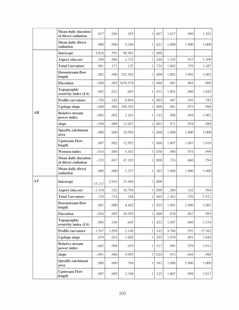
103
Mean daily duration of direct radiation .017 .040 .185 1 .667 1.017 .940 1.101
Mean daily direct radiation .000 .000 5.286 1 .021 1.000 1.000 1.000
Intercept 5.810 .591 96.481 1 .000
Aspect (sin.cos) .100 .086 1.332 1 .248 1.105 .933 1.309
Total Curvature .061 .171 .125 1 .724 1.062 .759 1.487
Downstream flow length .002 .000 241.502 1 .000 1.002 1.002 1.002
Elavation -.098 .002 3476.578 1 .000 .907 .904 .909
Topographic erosivity index (LS) .002 .022 .007 1 .931 1.002 .960 1.045
Profile curvature -.720 .242 8.864 1 .003 .487 .303 .782
Upslope slope -.040 .004 100.343 1 .000 .961 .953 .968
Relative stream power index -.002 .002 2.161 1 .142 .998 .994 1.001
slope -.030 .009 11.047 1 .001 .971 .954 .988
Specific catchment area .000 .000 18.956 1 .000 1.000 1.000 1.000
Upstream Flow length .007 .002 12.952 1 .000 1.007 1.003 1.010
Wetness index -.014 .006 4.402 1 .036 .986 .974 .999
Mean daily duration of direct radiation -.323 .047 47.192 1 .000 .724 .660 .794
AR
Mean daily direct radiation .000 .000 1.257 1 .262 1.000 1.000 1.000
Intercept -15.117 2.616 33.404 1 .000
Aspect (sin.cos) -1.318 .322 16.704 1 .000 .268 .142 .504
Total Curvature .310 .714 .188 1 .665 1.363 .336 5.521
Downstream flow length .001 .000 4.462 1 .035 1.001 1.000 1.001
Elavation -.024 .005 26.959 1 .000 .976 .967 .985
Topographic erosivity index (LS) .084 .104 .645 1 .422 1.087 .886 1.334
Profile curvature 1.547 1.058 2.140 1 .143 4.700 .591 37.362
Upslope slope .019 .014 1.682 1 .195 1.019 .991 1.048
Relative stream power index -.005 .008 .419 1 .517 .995 .979 1.011
slope -.091 .040 5.095 1 .024 .913 .844 .988
Specific catchment area .000 .000 .760 1 .383 1.000 1.000 1.000
AT
Upstream Flow length .007 .005 2.348 1 .125 1.007 .998 1.017

104
Wetness index -.045 .022 4.073 1 .044 .956 .915 .999
Mean daily duration of direct radiation 1.146 .211 29.477 1 .000 3.147 2.080 4.760
Mean daily direct radiation .000 .000 1.741 1 .187 1.000 1.000 1.000
Intercept 6.808 .499 185.933 1 .000
Aspect (sin.cos) .296 .072 16.943 1 .000 1.344 1.168 1.548
Total Curvature .038 .127 .091 1 .763 1.039 .810 1.332
Downstream flow length .002 .000 614.634 1 .000 1.002 1.002 1.003
Elavation -.048 .001 2018.033 1 .000 .953 .951 .955
Topographic erosivity index (LS) -.015 .013 1.289 1 .256 .985 .959 1.011
Profile curvature -.434 .183 5.625 1 .018 .648 .453 .927
Upslope slope -.038 .003 131.964 1 .000 .962 .956 .969
Relative stream power index -.001 .001 .526 1 .468 .999 .998 1.001
slope -.047 .006 52.113 1 .000 .954 .942 .967
Specific catchment area .000 .000 16.959 1 .000 1.000 1.000 1.000
Upstream Flow length .006 .002 13.172 1 .000 1.006 1.003 1.010
Wetness index -.008 .006 2.090 1 .148 .992 .980 1.003
Mean daily duration of direct radiation -.473 .041 132.482 1 .000 .623 .575 .675
CM
Mean daily direct radiation .000 .000 34.478 1 .000 1.000 1.000 1.000
Intercept 9.418 .618 232.199 1 .000
Aspect (sin.cos) .100 .097 1.054 1 .305 1.105 .913 1.336
Total Curvature 1.040 .186 31.188 1 .000 2.830 1.965 4.078
Downstream flow length .001 .000 106.500 1 .000 1.001 1.001 1.002
Elavation -.018 .001 177.408 1 .000 .982 .979 .984
Topographic erosivity index (LS) .111 .022 26.143 1 .000 1.117 1.071 1.165
Profile curvature 1.600 .266 36.168 1 .000 4.953 2.940 8.343
Upslope slope -.008 .004 4.574 1 .032 .992 .984 .999
Relative stream power index -.008 .002 23.633 1 .000 .992 .988 .995
slope -.182 .011 297.214 1 .000 .834 .817 .851
Specific catchment area .000 .000 1.082 1 .298 1.000 1.000 1.000
FL
Upstream Flow length .004 .002 4.199 1 .040 1.004 1.000 1.008

105
Wetness index .003 .007 .186 1 .667 1.003 .989 1.018
Mean daily duration of direct radiation -.999 .049 419.800 1 .000 .368 .335 .405
Mean daily direct radiation .000 .000 4.852 1 .028 1.000 1.000 1.000
Intercept 2.877 .738 15.209 1 .000
Aspect (sin.cos) .169 .106 2.539 1 .111 1.184 .962 1.458
Total Curvature .745 .246 9.161 1 .002 2.107 1.300 3.414
Downstream flow length .001 .000 46.574 1 .000 1.001 1.001 1.001
Elavation -.009 .002 33.066 1 .000 .991 .988 .994
Topographic erosivity index (LS) .124 .045 7.500 1 .006 1.132 1.036 1.236
Profile curvature 2.178 .357 37.266 1 .000 8.830 4.388 17.770
Upslope slope -.006 .005 1.407 1 .236 .994 .985 1.004
Relative stream power index -.015 .004 12.933 1 .000 .985 .977 .993
slope -.256 .016 257.052 1 .000 .774 .750 .799
Specific catchment area .000 .000 2.489 1 .115 1.000 1.000 1.000
Upstream Flow length .002 .002 .920 1 .338 1.002 .998 1.006
Wetness index -.003 .008 .175 1 .676 .997 .982 1.012
Mean daily duration of direct radiation -.222 .060 13.674 1 .000 .801 .712 .901
GL
Mean daily direct radiation .000 .000 16.017 1 .000 1.000 1.000 1.000
Intercept 5.008 .683 53.691 1 .000
Aspect (sin.cos) .073 .105 .486 1 .486 1.076 .876 1.322
Total Curvature 1.209 .212 32.389 1 .000 3.349 2.209 5.078
Downstream flow length .001 .000 18.392 1 .000 1.001 1.000 1.001
Elavation .006 .001 15.123 1 .000 1.006 1.003 1.009
Topographic erosivity index (LS) -.026 .026 .977 1 .323 .974 .926 1.026
Profile curvature 2.334 .308 57.246 1 .000 10.316 5.636 18.881
Upslope slope .023 .004 33.415 1 .000 1.023 1.015 1.031
Relative stream power index .000 .001 .010 1 .920 1.000 .998 1.003
slope -.207 .013 244.074 1 .000 .813 .792 .834
Specific catchment area .000 .000 .034 1 .853 1.000 1.000 1.000
HS
Upstream Flow length -.003 .002 1.629 1 .202 .997 .993 1.002

106
Wetness index .021 .008 7.062 1 .008 1.021 1.006 1.037
Mean daily duration of direct radiation -.544 .054 101.060 1 .000 .581 .522 .646
Mean daily direct radiation .000 .000 16.484 1 .000 1.000 1.000 1.000
Intercept -4.569 5.105 .801 1 .371
Aspect (sin.cos) .569 .391 2.114 1 .146 1.766 .820 3.802
Total Curvature .610 .711 .736 1 .391 1.841 .457 7.420
Downstream flow length -.004 .001 47.803 1 .000 .996 .995 .997
Elavation .050 .007 48.469 1 .000 1.051 1.036 1.066
Topographic erosivity index (LS) .023 .040 .351 1 .553 1.024 .947 1.106
Profile curvature 1.190 1.068 1.243 1 .265 3.288 .406 26.657
Upslope slope .010 .027 .135 1 .713 1.010 .959 1.064
Relative stream power index .001 .002 .144 1 .704 1.001 .997 1.005
slope -.075 .040 3.499 1 .061 .928 .858 1.004
Specific catchment area .000 .000 .408 1 .523 1.000 1.000 1.000
Upstream Flow length .014 .010 2.120 1 .145 1.014 .995 1.033
Wetness index -.046 .031 2.148 1 .143 .955 .899 1.016
Mean daily duration of direct radiation -.202 .275 .543 1 .461 .817 .477 1.400
LP
Mean daily direct radiation .000 .000 1.566 1 .211 1.000 1.000 1.000
Intercept 2.730 .522 27.371 1 .000
Aspect (sin.cos) .152 .074 4.152 1 .042 1.164 1.006 1.346
Total Curvature .496 .133 13.865 1 .000 1.642 1.265 2.131
Downstream flow length .001 .000 63.224 1 .000 1.001 1.001 1.001
Elavation -.022 .001 408.716 1 .000 .978 .976 .980
Topographic erosivity index (LS) .009 .013 .438 1 .508 1.009 .983 1.036
Profile curvature 1.264 .193 43.063 1 .000 3.539 2.426 5.161
Upslope slope .000 .003 .000 1 .986 1.000 .993 1.007
Relative stream power index .000 .001 .109 1 .742 1.000 .998 1.001
slope -.081 .007 143.832 1 .000 .922 .910 .934
Specific catchment area .000 .000 9.499 1 .002 1.000 1.000 1.000
LV
Upstream Flow length .003 .002 3.139 1 .076 1.003 1.000 1.007

107
Wetness index -.016 .006 6.954 1 .008 .984 .973 .996
Mean daily duration of direct radiation -.013 .043 .096 1 .756 .987 .907 1.074
Mean daily direct radiation .000 .000 10.912 1 .001 1.000 1.000 1.000
Intercept 10.332 2.052 25.349 1 .000
Aspect (sin.cos) -.706 .293 5.815 1 .016 .493 .278 .876
Total Curvature .193 .435 .196 1 .658 1.213 .517 2.845
Downstream flow length -.004 .000 93.943 1 .000 .996 .996 .997
Elavation .024 .004 34.758 1 .000 1.025 1.016 1.033
Topographic erosivity index (LS) .054 .035 2.487 1 .115 1.056 .987 1.130
Profile curvature .660 .648 1.039 1 .308 1.936 .544 6.889
Upslope slope .010 .012 .692 1 .406 1.010 .987 1.034
Relative stream power index -.001 .002 .318 1 .573 .999 .994 1.003
slope -.135 .028 23.847 1 .000 .873 .827 .922
Specific catchment area .000 .000 1.920 1 .166 1.000 1.000 1.000
Upstream Flow length .010 .006 2.518 1 .113 1.010 .998 1.022
Wetness index .039 .022 3.188 1 .074 1.039 .996 1.084
Mean daily duration of direct radiation -.712 .152 21.942 1 .000 .491 .364 .661
PH
Mean daily direct radiation .000 .000 32.723 1 .000 1.000 1.000 1.000
Intercept 4.632 .780 35.233 1 .000
Aspect (sin.cos) .051 .111 .213 1 .645 1.053 .847 1.308
Total Curvature .047 .191 .062 1 .804 1.049 .721 1.524
Downstream flow length -.001 .000 30.955 1 .000 .999 .999 .999
Elavation .004 .002 4.987 1 .026 1.004 1.000 1.007
Topographic erosivity index (LS) -.014 .022 .406 1 .524 .986 .945 1.029
Profile curvature .243 .275 .779 1 .377 1.275 .743 2.188
Upslope slope -.032 .006 26.687 1 .000 .969 .957 .981
Relative stream power index -.001 .002 .115 1 .734 .999 .997 1.002
slope -.008 .010 .634 1 .426 .992 .972 1.012
Specific catchment area .000 .000 5.718 1 .017 1.000 1.000 1.000
PZ
Upstream Flow length .010 .003 14.282 1 .000 1.010 1.005 1.015

108
Wetness index -.040 .009 18.397 1 .000 .960 .943 .978
Mean daily duration of direct radiation -.285 .063 20.320 1 .000 .752 .664 .851
Mean daily direct radiation .000 .000 25.785 1 .000 1.000 1.000 1.000
Intercept -9.309 1.583 34.588 1 .000
Aspect (sin.cos) -.073 .194 .141 1 .707 .930 .635 1.361
Total Curvature .668 .449 2.213 1 .137 1.951 .809 4.703
Downstream flow length .001 .000 20.259 1 .000 1.001 1.001 1.001
Elavation .005 .003 3.423 1 .064 1.005 1.000 1.011
Topographic erosivity index (LS) .047 .073 .418 1 .518 1.048 .909 1.209
Profile curvature 2.324 .667 12.139 1 .000 10.211 2.763 37.734
Upslope slope -.005 .011 .179 1 .672 .995 .973 1.018
Relative stream power index -.004 .005 .590 1 .443 .996 .986 1.006
slope -.148 .028 27.208 1 .000 .862 .815 .912
Specific catchment area .000 .000 1.483 1 .223 1.000 1.000 1.000
Upstream Flow length .005 .005 .798 1 .372 1.005 .994 1.015
Wetness index -.008 .015 .270 1 .604 .992 .965 1.021
Mean daily duration of direct radiation .543 .127 18.167 1 .000 1.721 1.341 2.209
RG
Mean daily direct radiation .000 .000 .569 1 .450 1.000 1.000 1.000
Intercept 7.723 .605 162.774 1 .000
Aspect (sin.cos) .639 .089 51.974 1 .000 1.894 1.592 2.253
Total Curvature .167 .159 1.103 1 .294 1.182 .865 1.614
Downstream flow length -.001 .000 21.844 1 .000 .999 .999 1.000
Elavation -.034 .001 634.469 1 .000 .967 .964 .969
Topographic erosivity index (LS) -.014 .015 .891 1 .345 .986 .958 1.015
Profile curvature .367 .229 2.572 1 .109 1.443 .922 2.259
Upslope slope -.014 .004 12.378 1 .000 .986 .979 .994
Relative stream power index .001 .001 .596 1 .440 1.001 .999 1.002
slope -.040 .008 26.583 1 .000 .961 .946 .975
Specific catchment area .000 .000 11.950 1 .001 1.000 1.000 1.000
RGah
Upstream Flow length .006 .002 10.953 1 .001 1.006 1.003 1.010

109
Wetness index -.011 .007 2.545 1 .111 .989 .976 1.003
Mean daily duration of direct radiation -.362 .049 54.634 1 .000 .696 .632 .766
Mean daily direct radiation .000 .000 1.852 1 .174 1.000 1.000 1.000
a The reference category is: UM.


