+ All Categories
Home > Documents > The Asymptotic Behaviour of the Riemann Mapping Function at Analytic … · 2016-05-18 · ection...

The Asymptotic Behaviour of the Riemann Mapping Function at Analytic … · 2016-05-18 · ection...

Date post: 20-Mar-2020
Category:
Upload: others
View: 4 times
Download: 0 times
Share this document with a friend
97
Dissertation The Asymptotic Behaviour of the Riemann Mapping Function at Analytic Cusps Submitted to the Faculty of Computer Science and Mathematics of the University of Passau in Partial Fulfilment of the Requirements for the Degree Doctor Rerum Naturalium Sabrina Lehner February 2016
Transcript

Dissertation

The Asymptotic Behaviour of the RiemannMapping Function at Analytic Cusps

Submitted to the Faculty of Computer Science and Mathematics

of the University of Passau in Partial Fulfilment of the Requirements

for the Degree Doctor Rerum Naturalium

Sabrina Lehner

February 2016

Thesis Advisor: Prof. Dr. Tobias Kaiser Professorship of Mathematics,Faculty of Computer Science and Mathematics,University of Passau

External Referee: Prof. Dr. Oliver Roth Chair of Complex Analysis,Department of Mathematics,Julius-Maximilians-University of Wurzburg

Acknowledgements

Completing this thesis was an unforgettable experience and would not have been possible

without the support of many outstanding people at the University of Passau and beyond.

Therefore, it is a real pleasure for me to hereby take the opportunity and express my

gratitude to them.

First of all, I would like to thank Prof. Dr. Tobias Kaiser, my supervisor, for his

continuous support, advise, and encouragements throughout the course of my PhD. This

work would certainly not have been realisable without his great guidance and constant

feedback. Moreover, I would like to thank Prof. Dr. Oliver Roth who kindly agreed to

be the external reviewer of my thesis. It was also a real pleasure to follow his invitation

to visit the University of Wurzburg for giving a talk at his seminar and thereby to get

to know his team at the Chair of Complex Analysis.

I also want to express my acknowledgements to Prof. Dr. Tobias Kaiser and Prof. Dr.

Niels Schwartz for organising the seminar ”Reelle Algebra und Reelle Geometrie” which

provided an effective scientific environment. It gave me the opportunity to gain insights

into mathematical research areas beyond my own topic and allowed me to present as

well as discuss my results which was a great help for developing new ideas.

Furthermore, I would like to thank Prof. Dr. Wolfgang Lauf from the OTH Regensburg

for organising a PhD seminar in 2014 and for giving me the opportunity to present my

work there.

At this point a kind word of appreciation to the Deutsche Forschungsgemeinschaft

(DFG) for financing my position as a PhD student in the context of the project “O-

minimal Structures and their Applications to Dynamical Systems, Complex Analysis,

i

Acknowledgements

and Potential Theory” (KA 3297/1). Additionally, my sincere thanks to the University

of Passau for the financial support during the final months of my PhD provided by

the “Bavarian Equal Opportunities Sponsorship – Promoting Equal Opportunities for

Women in Research and Teaching” (Bayerische Gleichstellungsforderung).

Special thanks go as well to my colleagues and friends at the University of Passau who

made my time as a PhD student highly enjoyable and without whom this experience

would have been surely incomplete. In particular, I want to mention my friend and office

colleague Julia Ruppert and our secretary Rita Saxinger who was always there to help

with organisational issues.

I would like to express my deepest gratitude to my parents Ingrid and Alois, and my

brother Dominic. Thank you for your never-ending love, encouragements and support

in all my pursuits, and for the countless opportunities you have given me in life. Special

thanks also to my aunt Marianne and my uncle Johann, my grandparents Mathilde

and Karl, and my grandmother Marianne for her never-ending chocolate supply. They

all stood by my side and shared with me both great and difficult moments of life.

Furthermore, I want to thank Christine, Michael, and David for the enjoyable moments

we shared in the last few years.

Finally, I would like to thank Philipp for his immense support throughout the whole

time. Thank you for proof-reading and helpful discussions, for your honesty and patience.

I owe you much more than I would ever be able to express, so I keep it plain and simple:

thank you so much for your love and care!

Sabrina Lehner

Passau, February 2016

ii

Contents

Acknowledgements i

Notation v

1 Introduction 1

1.1 Motivation . . . . . . . . . . . . . . . . . . . . . . . . . . . . . . . . . . . 1

1.2 Outline and Research Contributions . . . . . . . . . . . . . . . . . . . . . 4

2 Preliminaries 9

2.1 Basic Definitions and Lemmas . . . . . . . . . . . . . . . . . . . . . . . . . 9

2.2 The Riemann Mapping Theorem . . . . . . . . . . . . . . . . . . . . . . . 15

2.3 Classification of Boundary Points . . . . . . . . . . . . . . . . . . . . . . . 17

2.4 Asymptotic Behaviour at Analytically Regular Boundary Points . . . . . 19

2.4.1 Schwarz Reflection . . . . . . . . . . . . . . . . . . . . . . . . . . . 19

2.4.2 General Premises . . . . . . . . . . . . . . . . . . . . . . . . . . . . 21

2.4.3 Asymptotic Behaviour . . . . . . . . . . . . . . . . . . . . . . . . . 21

2.5 Asymptotic Behaviour at Analytic Corners . . . . . . . . . . . . . . . . . 22

2.5.1 General Premises . . . . . . . . . . . . . . . . . . . . . . . . . . . . 23

2.5.2 Asymptotic Behaviour of the Mapping Function and its Inverse . . 24

2.5.3 Development in a Generalised Power Series . . . . . . . . . . . . . 25

2.6 O-minimal Structures . . . . . . . . . . . . . . . . . . . . . . . . . . . . . 27

2.6.1 Definitions . . . . . . . . . . . . . . . . . . . . . . . . . . . . . . . 28

2.6.2 Examples . . . . . . . . . . . . . . . . . . . . . . . . . . . . . . . . 30

iii

Contents

2.6.3 O-minimal Content of the Riemann Mapping Theorem . . . . . . . 31

3 Asymptotic Behaviour at Analytic Cusps 33

3.1 General Premises . . . . . . . . . . . . . . . . . . . . . . . . . . . . . . . . 34

3.2 Small Perturbation of Angles . . . . . . . . . . . . . . . . . . . . . . . . . 37

3.3 Preliminary Transformation . . . . . . . . . . . . . . . . . . . . . . . . . . 38

3.4 Estimates for the Modulus and the Argument . . . . . . . . . . . . . . . . 41

3.5 Asymptotic Behaviour of the Riemann map . . . . . . . . . . . . . . . . . 54

3.6 Asymptotic Behaviour of the Derivatives . . . . . . . . . . . . . . . . . . . 60

3.7 Asymptotic Behaviour of the Inverse . . . . . . . . . . . . . . . . . . . . . 70

3.8 Asymptotic Behaviour of the Derivatives of the Inverse . . . . . . . . . . . 72

4 Future Research 79

List of Figures 83

Bibliography 85

iv

Notation

N := 1, 2, . . . set of natural numbers

N0 := N ∪ 0 set of nonnegative integers

R field of real numbers

R∗ := R \ 0 set of real numbers without 0

R≥0 := x ∈ R | x ≥ 0 set of positive real numbers

R≤0 := x ∈ R | x ≤ 0 set of negative real numbers

C := x+ iy | x, y ∈ R field of complex numbers

C∗ := C \ 0 set of complex numbers without 0

C− := C \ R≤0 slit plane

H := z ∈ C | Im(z) > 0 upper half plane

H− := z ∈ C | Im(z) < 0 lower half plane

E := z ∈ C | |z| < 1 open Euclidian unit disk with radius 1

and center 0

E1 := z ∈ C | |z − 1| < 1 open Euclidean unit disk with radius 1

and center 1

B(a, r) := z ∈ C | |z − a| < r open Euclidean disk with radius r > 0

and center a ∈ C

B(a, r) := z ∈ C | |z − a| ≤ r closed Euclidean disk with radius r > 0

and center a ∈ C

A closure of a set A ⊂ CA interior of a set A ⊂ C

∂A := A \A boundary of a set A ⊂ C

v

Notation

Re(z), Im(z) real and imaginary part of z ∈ C

Re(f), Im(f) real and imaginary part of a complex-valued

function f

|z| modulus, absolute value of z ∈ C

graph(f) graph of a function f

R[x1, . . . , xn] real polynomial ring in n variabels

arg(z) ∈ ]− π, π] standard argument of z ∈ C∗

dist(w, z) := |w − z| Euclidean distance of w, z ∈ C

vi

Chapter 1

Introduction

1.1 Motivation

Geometric function theory is a branch of complex analysis and studies geometric prop-

erties of analytic functions. While complex analysis has its roots in the 19th century,

the origins of geometric function theory can be traced back to the beginning of the 20th

century. Among other topics, it is dealing with conformal maps and analytic continua-

tion. One of the fundamental theorems in this branch of mathematics is the Riemann

Mapping Theorem. It states the existence of a conformal map between a simply con-

nected proper domain of the complex plane and the unit disk. In fact, this theorem was

the beginning of the study of complex analysis from a geometric point of view and the

names of many mathematicians are linked to the history of it. In 1851, Riemann stated

the theorem in his PhD thesis ”Grundlagen fur eine allgemeine Theorie der Functionen

einer veranderlichen complexen Grosse”, see Riemann [18], and sketched a proof for

bounded domains with piecewise smooth boundary based on the Dirichlet principle. In

1870, however, Weierstraß showed that the Dirichlet principle was not valid for domains

with general boundary and concluded that there may not exist a minimum as Riemann

assumed in his proof. The criticism of Weierstraß on the Dirichlet principle was weak-

ened in 1904 as David Hilbert proved the Dirichlet principle to the extent required by

Riemann and so the validity of Riemann’s proof of the theorem was restored. In the

1

Chapter 1 Introduction

meantime many new methods were developed for proving the Riemann Mapping Theo-

rem. For instance, in 1870 a student of Weierstraß, Hermann Amandus Schwarz, gave a

proof of the Riemann Mapping Theorem for the case of simply connected domains with

piecewise analytic boundary by showing that the Green’s function exists under these

assumptions, see Schwarz [20]. Another well known proof was performed by Osgood in

1900. He showed the theorem for simply connected domains with an arbitrary boundary

by proving the existence of the Green’s function corresponding to the domain, see Os-

good [14]. A common way to prove the Riemann Mapping Theorem nowadays is through

the use of the Theorem of Montel [6, Theorem IV.4.9 on p. 236]. For an overview on the

history of the proofs for the Riemann Mapping Theorem we refer to Gray [7].

An important question that arises in the context of the Riemann Mapping Theorem

is the following: what can we say about the extendability of a conformal map to the

boundary? Constantin Caratheodory, a mathematician of Greek origin, worked on topics

related to this question and achieved pioneering results. In 1913, he proved that a

conformal map of a domain which is bounded by a Jordan arc onto the unit disk has

a continuous and bijective continuation to the boundaries. This conjecture was given

earlier by William Fogg Osgood.

The topic of this work originates from the field of geometric function theory and

is concerned with the asymptotic behaviour of conformal mappings at the boundary.

This means we want to describe their behaviour by well-known, elementary functions.

Motivated by real analytic geometry we assume that the boundary is piecewise analytic.

There are two cases we have to distinguish: the behaviour at regular boundary points

and the behaviour at singular boundary points. If we have a regular boundary point,

we can determine the asymptotic behaviour of the mapping function at this point by

the Schwarz Reflection at analytic arcs, a technique for analytic continuation. If we

have a singular boundary point, we have to distinguish analytic corners, where the

opening angle of two regular analytic arcs is greater than 0, and analytic cusps, where

the opening angle vanishes. The asymptotic behaviour of conformal mapping functions

at analytic corners has been already studied extensively. For instance, Leon Lichtenstein

2

1.1 Motivation

and Stephan Emanuel Warschawski focussed on the behaviour of the mapping function

and its derivatives at analytic corners, see Lichtenstein [13] and Warschawski [22]. While

Lichtenstein concentrated on a special case regarding the asymptotic behaviour of the

derivates, Warschawski generalised these results.

A much stronger result than Lichtenstein and Warschawski was stated by Russell

Sherman Lehman in 1957. He showed that the mapping function can be developed in

a certain generalised power series, see Lehman [11]. This result was used to investi-

gate geometric statements of the Riemann Mapping Theorem related to real analytic

geometry: on the basis of Lehman’s result, Tobias Kaiser investigated in 2009, see [8],

the o-minimal content of the Riemann Mapping Theorem by proving that the mapping

functions of semianalytic domains without cusps are in many cases definable in an o-

minimal structure. O-minimal structures generalise the geometry of algebraic character.

In the early 80’s Lou van den Dries et al. isolated one property of ordered structures

that leads to tame behaviour, the so-called o-minimality property. Important concepts

and functions from analysis can be realised in o-minimal structures which are defined

by nice tameness- and finitness-properties. A natural question arising from this “tame”

point of view is if it is also possible to make a statement for domains with analytic

cusps similar to the one Kaiser proved for domains with analytic corners by using the

generalised power series.

While there are many results on the asymptotic behaviour at analytic corners, there

are only a few articles that deal with the asymptotic behaviour of mapping functions

at analytic cusps. One is from Warschawski who works in a more general setting than

that of analytic cusps. A second result was published in 2010 by Kaiser [9] where he

investigated the behaviour of the mapping function at analytic cusps for domains with

small perturbation of angles and gave upper bounds for its derivatives. However, to

this day there is still a knowledge gap and many questions related to the asymptotic

behaviour of such mapping functions at analytic cusps remain unanswered. Therefore,

the goal of this work is to discuss the asymptotic behaviour at analytic cusps in a more

general setting than that of domains with small perturbation of angles. Furthermore,

3

Chapter 1 Introduction

we investigate the behaviour of its derivatives, its inverse, and of the derivatives of its

inverse. Based on these results we also give a conjecture on the asymptotic power series

expansion for the inverse function.

1.2 Outline and Research Contributions

In Chapter 2, we initiate basic terminology of complex analysis required later on in

the thesis. The well known Riemann Mapping Theorem that gives us the existence of

a conformal map of a simply connected proper domain of the complex plane onto the

unit disk is presented in Section 2.2. We recall Caratheodory’s important Prime End

Theorem on the extension of conformal maps to the boundary in Section 2.3. It is one of

the main topics in geometric function theory to understand the behaviour of such maps

at the boundary. In this work, we concentrate on piecewise analytic boundaries which

means that the boundary of our simply connected proper domain of the complex plane

consists of a finite number of analytic arcs. Section 2.3 contains a classification for the

different boundary points, namely singular and regular boundary points, and introduces

analytic corners and analytic cusps. The next part of this chapter, Section 2.4, covers

the asymptotic behaviour of a Riemann map at regular boundary points: we recall two

techniques for analytic continuation, namely the Schwarz Reflection Principle and the

Schwarz Reflection at analytic arcs, and by using the latter one can show that a given

mapping function behaves like z at a regular boundary point. Section 2.5 focusses on

the behaviour of a Riemann map at an analytic corner which means that the opening

angle between two regular analytic arcs is greater than 0. We present the results of

Lichtenstein, Warschawski, and Lehman on the asymptotic behaviour of the Riemann

map of a simply connected domain with an analytic corner onto the upper half plane

and on estimates for its derivatives. Especially, the result of Lehman is fundamental

since he showed that the mapping function can be developed in a certain generalised

power series. On the basis of this result Kaiser proved that the mapping functions

of semianalytic domains without cusps are in many cases definable in an o-minimal

4

1.2 Outline and Research Contributions

structure. Section 2.6 gives an overview on the basic concepts of o-minimal structures,

presents some concrete examples for the latter, and recalls the above mentioned theorem

of Kaiser.

Chapter 3 starts with general premises, see Section 3.1, where we introduce basic no-

tation. Moreover, we see that by applying a translation we can focus on the case that

we have a simply connected proper domain of the complex plane with an analytic cusp

at 0. In Section 3.2, we present the results of Kaiser for the asymptotic behaviour of a

Riemann map in the situation that the domain has small perturbation of angles. After

applying a preliminary transformation to our domain, we investigate the asymptotic

behaviour of the Riemann map for the case that one of the two boundary arcs in some

neighbourhood of the cusp at 0 coincides with the positive real axis, see Section 3.3.

We denote such a domain by Ω. In Section 3.4, we present a theorem of Warschawski

on the modulus and the argument of a conformal map of a simply connected proper

domain of the complex plane onto the unit disk with center 1 in a neighbourhood of

0. Furthermore, we give a remark on the estimates for the modulus and the argument

of the conformal map if the latter domain is mapped onto the upper half plane instead

of mapping it onto the unit disk with center 1. By adapting this theorem to our case,

we can therefore give estimates for the modulus and the argument of our Riemann map

ϕ : Ω→ H with ϕ(0) = 0 at the analytic cusp at 0. We introduce the asymptotic tuple

of Ω which consists of geometric invariants depending on the shape of the domain Ω at

the cusp. As a first main result we prove the following corollary.

Corollary

We have

(a)

|ϕ(z)| = c exp

(|z|−d

d−1∑

n=0

bn|z|n + a log |z|+ o(1)

)

where c ∈ R>0 is a constant and (b0, . . . , bd−1, a) ∈ Rd+1 is the asymptotic tuple

of Ω.

5

Chapter 1 Introduction

(b)

arg(ϕ(z)) = π arg(z)|z|−d(

d∑

n=0

cn|z|n)

+ o(1).

Based on this result we prove in Section 3.5 the following theorem on the asymptotic

behaviour of ϕ at 0.

Theorem A

We have

ϕ(z) ∼ za exp

(b0zd

+b1zd−1

+ · · ·+ bd−1

z

)

at 0 on Ω where (b0, . . . , bd−1, a) is the asymptotic tuple of Ω.

Moreover, we give an example and discuss the special situation where a = 0. That

is particularly interesting as this is the case when Ω has small perturbation of angles.

Furthermore, we determine in Section 3.6 the asymptotic behaviour of the derivatives

ϕ(n) for n ∈ N.

Theorem B

Let n ∈ N0. Then

ϕ(n)(z) ∼ ϕ(z)z−n(d+1) ∼ za−n(d+1) exp

(b0zd

+ · · ·+ bd−1

z

)

at 0 on Ω where (b0, . . . , bd−1, a) is the asymptotic tuple of Ω.

By using these results, we subsequently study in Section 3.7 the behaviour of the inverse

mapping function ψ : H→ Ω of the Riemann map ϕ. Moreover, we have again ψ(0) = 0.

Theorem C

We have at 0 on H

ψ(z) '(− π

add log(|z|)

) 1d

.

6

1.2 Outline and Research Contributions

In Section 3.8, we investigate the behaviour of the derivatives of the inverse and obtain

the following theorem.

Theorem D

Let n ∈ N. Then

ψ(n)(z) ∼ (ψ(z))d+1z−n ∼(− 1

log(z)

) 1d

+1

z−n

at 0 on H.

Finally, Chapter 4 concludes the thesis by giving an outlook on future work. In continu-

ation of the research presented in this thesis, it is the goal to derive a generalised power

series for the mapping function ϕ analogously to the result of Lehman for analytic cor-

ners. We therefore present a conjecture on the asymptotic power series expansion of ψ

at 0 in a special case and give an idea of the proof. By verifying this conjecture it would

be immediately possible to determine the asymptotic power series expansion of ϕ.

7

Chapter 2

Preliminaries

2.1 Basic Definitions and Lemmas

In this section we present some basic definitions and lemmas required later on in the

thesis. If not stated otherwise we follow the definitions as given in Ahlfors [1], Freitag

and Busam [6], Kaiser [9], Lang [10], and Pommerenke [16].

Definition 2.1.1

Let U ⊂ C be an open set and let f : U → C. The function f is called analytic at

z0 ∈ U if there exists a power series

∞∑

n=0

an(z − z0)n

and some r > 0 such that the series converges absolutely for z ∈ B(z0, r), and such that

we have

f(z) =∞∑

n=0

an(z − z0)n

for all z ∈ B(z0, r). The function f is called analytic in U if f is analytic at every

z ∈ U .

Definition 2.1.2

Let U ⊂ C be an open, nonempty set and let a, b ∈ R with a < b. A curve in U is a

9

Chapter 2 Preliminaries

continuous map of the form

γ : [a, b]→ U, t 7→ γ(t).

Moreover, γ(a) is called the beginning point and γ(b) the endpoint. A curve γ is

called closed if γ(a) = γ(b).

Definition 2.1.3

We say that a curve γ : [a, b]→ C is regular at t0 ∈ [a, b] if γ is differentiable at t0 and

γ′(t0) 6= 0. The curve γ is called regular if it is regular at every point. We say that γ

is singular at t0 if γ is differentiable at t0 and γ′(t0) = 0.

Definition 2.1.4

A curve γ : [a, b]→ C is called a simple closed curve or a Jordan curve if γ is closed

and γ(s) 6= γ(t) for all s, t ∈ [a, b] with s < t and t− s < b− a.

Definition 2.1.5

A curve γ : [a, b] → C is called real analytic if for each point t0 ∈ [a, b] there exists a

convergent power series expansion

γ(t) =

∞∑

n=0

an(t− t0)n

for all t sufficiently close to t0.

Definition 2.1.6

A curve is called smooth if it is continuously differentiable.

Definition 2.1.7

A curve γ : [a, b]→ C is called piecewise smooth if there is a partition a = a0 < a1 <

· · · < an = b of the interval [a, b] such that the restrictions γν := γ|[aν ,aν+1] are smooth

for 0 ≤ ν < n.

10

2.1 Basic Definitions and Lemmas

Definition 2.1.8

Let γ : [a, b]→ C be a curve. The trace of the curve γ is denoted by tr(γ) := γ([a, b]) ⊂ C

and is called an arc (parameterised by γ).

Definition 2.1.9

An arc Γ is called regular at P ∈ Γ if there exists locally a parameterisation γ of Γ

with γ(t0) = P such that γ is regular at t0. Otherwise Γ is singular at P . An arc Γ is

called regular if Γ is regular at every point.

Definition 2.1.10

The trace of a Jordan curve is called a Jordan arc.

Definition 2.1.11

An arc Γ is said to be an analytic arc at P ∈ Γ if Γ has a real analytic parameterisation

in some neighbourhood U ⊂ C of P , i.e. there exists a real analytic curve γ :]− ε, ε[→ U

such that γ(0) = P , γ :]− ε, ε[→ γ(]− ε, ε[) is injective and U ∩ Γ = γ(]− ε, ε[). An arc

Γ is said to be an analytic arc if this property holds for every point P ∈ Γ.

Definition 2.1.12

An arc Γ is said to be piecewise (regular) analytic if it can be decomposed into a

finite number of arcs Γ1, . . . ,Γn, n ∈ N, such that there exists for every i ∈ 1, . . . , n a

real analytic (regular) curve γi :]− εi, εi[→ C and a compact intervall Ii ⊂]− εi, εi[ with

Γi = γi(Ii).

Definition 2.1.13

A set A ⊂ C is called arcwise connected if for any two points w, z ∈ A there is a

piecewise smooth curve γ : [a, b]→ A such that

γ(a) = w, γ(b) = z.

Definition 2.1.14

Let U ⊂ C be an open set. U is called a domain if it is nonempty and arcwise connected.

11

Chapter 2 Preliminaries

Definition 2.1.15

A domain G ⊂ C is called simply connected if the closed set C \ G has no bounded

connected components.

Definition 2.1.16

A map ϕ : U → V between two open sets U, V ⊂ C is called conformal iff the following

conditions are satisfied

(a) ϕ is bijective,

(b) ϕ is analytic,

(c) ϕ−1 is analytic.

The geometrical significance of a conformal map ϕ is that the oriented angle between

the traces of two regular curves γ1 and γ2 at an intersection point a ∈ U is equal to the

oriented angle between the arcs tr(ϕ γ1) and tr(ϕ γ2) at their intersection point ϕ(a).

Definition 2.1.17

Given a non-vanishing real or complex power series h(t) =∞∑n=0

antn we set

ord(h) := minn ∈ N0 : an 6= 0

which is called the order of the power series. Moreover, we set ord(0) :=∞.

To describe the asymptotic behaviour of a mapping function we need some further

notation. Suppose we have a function f and want to consider how quickly the function

goes to 0 near 0. Then we would like to find a simple function g which also vanishes at

0 such that g and f are almost equal near 0.

Definition 2.1.18

Let A ⊂ C be a nonempty set with 0 ∈ A, let f, g : A→ C and let g(z) 6= 0 for all z in

a neighbourhood of 0. We write

12

2.1 Basic Definitions and Lemmas

(a) f ' g at 0 on A if

limz→0

f(z)

g(z)= 1,

(b) f ∼ g at 0 on A if

limz→0

f(z)

g(z)∈ C∗,

(c) f = o(g) at 0 on A if

limz→0

f(z)

g(z)= 0,

(d) f = O(g) at 0 on A if there is a C > 0 such that

|f(z)| ≤ C|g(z)|

for all z in a neighbourhood of 0.

The first two notation, (a) and (b), describe the situation where the function f is

asymptotically similar and asymptotically equivalent, respectively, to g around

0. Graphically, the o-notation describes that f goes much faster to 0 around 0 than g.

The well-known O-notation characterises functions according to their growth rate which

is often referred to as the order of the function. A description in terms of O-notation

provides an upper bound on the growth rate of the function. It is commonly used to

describe how closely a finite series approximates a given function. The function g is

typically chosen to be as simple as possible and is often used to describe the error term

in an approximation to a mathematical function. This means we do not know the exact

form of the error term but we have pointed out how small it is near 0. The little o-

notation makes a stronger statement than the corresponding big O-notation since every

function f that is o(g) is also O(g) near 0.

Remark 2.1.19

Note that the representation f = O(g) and f = o(g), respectively, is a slight abuse of

notation which is commonly used to express f ∈ O(g) and f ∈ o(g), respectively.

13

Chapter 2 Preliminaries

Lemma 2.1.20

Let A ⊂ C with A 6= ∅ and 0 ∈ A and let f, g : A→ C be functions with g(z) 6= 0 for all

z in a neighbourhood of 0. If f = g + o(1) then exp(f) ' exp(g).

Proof: We have

f(z) = g(z) + o(1)⇔ f(z)− g(z) = o(1)

⇔ limz→0

(f(z)− g(z)) = 0

⇒ limz→0

exp(f(z)− g(z)) = 1

⇔ limz→0

exp(f(z))

exp(g(z))= 1

⇔ exp(f(z)) ' exp(g(z)).

Lemma 2.1.21

Let A ⊂ C be a domain with 0 ∈ ∂A and let f, g : A → C be analytic functions with

g(z) 6= 0 for all z in a neighbourhood of 0. Furthermore, we assume that limz→0

f(z) = 0 =

limz→0

g(z). Moreover, let f(z) ∼ g(z). Then we have

log(f) ' log(g).

Proof: Since f(z) ∼ g(z) we have

limz→0

f(z)

g(z)∈ C∗.

Thus there exists an analytic function ξ : A → C with limz→0

ξ(z) ∈ C∗ such that f(z) =

g(z)ξ(z). Applying the logarithm we get for l(z) ∈ −1, 0, 1 that

log(f(z)) = log(g(z)ξ(z)) = log(g(z)) + log(ξ(z)) + 2πil(z).

14

2.2 The Riemann Mapping Theorem

Since limz→0

log(ξ(z)) ∈ C and limz→0

1log(g(z)) = 0 it follows that

limz→0

log(f(z))

log(g(z))= lim

z→0

log(g(z)) + log(ξ(z)) + 2πil(z)

log(g(z))

= limz→0

(log(g(z))

log(g(z))+

log(ξ(z)) + 2πil(z)

log(g(z))

)

= 1 + limz→0

log(ξ(z)) + 2πil(z)

log(g(z))

= 1.

2.2 The Riemann Mapping Theorem

As initially mentioned, one of the most important theorems in geometric function theory

is the Riemann Mapping Theorem. This theorem gives the existence of a conformal

mapping function of a simply connected domain which is a proper subset of the complex

plane to the unit disk.

Theorem 2.2.1 (Riemann 1851)

Let Ω ( C be a simply connected domain. Then there exists a conformal map ϕ : Ω→ E.

Proof: We refer to Remmert [17, p. 175 f.].

In the following, we refer to such a map as a Riemann map. An example can be

seen in Figure 2.1.

The Riemann Mapping Theorem implies that any two simply connected proper do-

mains of the complex plain, which can be highly complicated, can be mapped conformally

onto each other. While it assures the existence of such a conformal mapping, it is not of

much help when we are faced with the practical problem of finding the mapping function

which transforms two given domains onto each other. Even if we consider a map from

the interior of a circle to the interior of a square, which is a relatively simple conformal

15

Chapter 2 Preliminaries

Re

Im

Ω

ϕ

Re

Im

E

Figure 2.1: Example of a Riemann map ϕ

map, we have no explicit formula using only elementary functions. The necessity thus

arises to develop special techniques which help with the treatment of a given mapping

problem. It is sufficient to adapt these techniques to the case in which one of the do-

mains is the unit disk since if we can map two domains onto the same disk, we can

also map them onto each other. Furthermore, it is an equivalent problem to consider a

conformal map onto the upper half plane instead of the unit disk which is a composition

of a Riemann map with a Mobius transformation. This transformation which maps the

unit disk onto the upper half plane is the so-called Cayley transformation, given in the

next definition.

Definition 2.2.2

(a) The map hC : C→ C defined by

hC(z) =z − iz + i

is called the Cayley transformation and maps the upper half plane conformally

onto the unit disk, i.e. hC(H) = E.

16

2.3 Classification of Boundary Points

(b) The map hC′ : C→ C given by

hC′(z) = i1 + z

1− z

is the inverse of the Cayley transformation. In particular, note that hC′(E) = H.

2.3 Classification of Boundary Points

Since we want to investigate the asymptotic behaviour of a Riemann map at special

boundary points later on, we have to examine the criteria for extending a Riemann

map to the boundary and discuss the different types of boundary points. Osgood first

conjectured that a Riemann map can be extended continuously to the boundary if the

boundary of the domain is a Jordan arc, we refer to Osgood [15]. As already men-

tioned, this conjecture was proven by Caratheodory in 1913, see [2], and is often called

Caratheodory’s Prime End Theorem. We recall this result below.

Theorem 2.3.1 (Caratheodory’s Prime End Theorem)

Let Ω ( C be a simply connected domain and let ∂Ω be a Jordan arc. Then the Rie-

mann map

ϕ : Ω→ E

extends continuously to the boundary, giving a homeomorphism

φ : ∂Ω→ ∂E.

Proof: We refer to Caratheodory [2].

This theorem implies that a Riemann map between two simply connected domains in

the complex plain whose boundaries are Jordan arcs can be extended to a homeomor-

phism of their closures. The next step is to have a closer look at the different kinds

of boundary points. In the following, let Ω ( C be a simply connected domain whose

boundary ∂Ω is a Jordan arc and is piecewise analytic and regular.

17

Chapter 2 Preliminaries

Definition 2.3.2

If there exists locally a parameterisation γ : [a, b]→ C of ∂Ω, t0 ∈ [a, b] with γ(t0) = P

and γ regular at t0 we say that Ω has a regular boundary point at P . Otherwise we

say that Ω has a singular boundary point at γ(t0).

The opening angle between two regular analytic arcs, intersecting at one point, is

the opening angle between the tangents of the arcs at the intersection point, see for

example Figure 2.2 where the blue half lines are the tangents. We assume that 0 ∈ ∂Ω,

otherwise we apply a translation. If 0 is a singular boundary point, the interior angle

of Ω at 0 is the opening angle between the two regular analytic arcs of ∂Ω at 0 which

has a nonempty intersection with Ω. We have to distinguish two cases:

1. Ω has an analytic corner at 0.

2. Ω has an analytic cusp at 0.

Definition 2.3.3

We say that Ω has an analytic corner at 0 if 0 is a singular boundary point and the

boundary at 0 is locally given by two regular analytic arcs with interior angle πα where

0 < α ≤ 2.

For an example of an analytic corner at 0, see Figure 2.2.

0 πα

Figure 2.2: Analytic corner at 0 with opening angle πα where 0 < α ≤ 2

18

2.4 Asymptotic Behaviour at Analytically Regular Boundary Points

Definition 2.3.4

We say that Ω has an analytic cusp at 0 if the boundary of Ω at 0 is locally given by

two regular analytic arcs such that the interior angle at 0 vanishes.

An example of an analytic cusp at 0 is depicted in Figure 2.3.

0

Figure 2.3: Analytic cusp at 0

The following holds for analytic corners and analytic cusps at 0, respectively: since

the boundary of Ω in a neighbourhood of 0 consists of two regular analytic arcs, which

we denote by Γ1 and Γ2, there exists some ε > 0 such that the parameterisations of the

boundary arcs are analytic on B(0, ε) and such that ∂Ω close to 0 is given by Γ1∪Γ2. We

denote these parameterisations by γ1 and γ2 where Γ1 := γ1([0, ε[) and Γ2 := γ2([0, ε[),

respectively. Since Γ1 and Γ2 are regular by assumption, we may assume that γ1 and γ2

are regular. Thus, γ′1(0)γ′2(0) 6= 0 holds. Moreover, we have γ1(0) = γ2(0) = 0.

2.4 Asymptotic Behaviour at Analytically Regular Boundary Points

In this section, we investigate the asymptotic behaviour of a Riemann map at an analyt-

ically regular boundary point. In this particular case, we can use the Schwarz Reflection

at analytic arcs, a technique for analytic continuation to extend the domain of definition

of an analytic function.

2.4.1 Schwarz Reflection

First, we recall the so-called Symmetry Principle or Schwarz Reflection Principle which

enables one to find a continuation easily and explicitly under rather special conditions.

19

Chapter 2 Preliminaries

Theorem 2.4.1 (Schwarz Reflection Principle)

Let G+ ⊂ H be a domain and suppose that the boundary of G+ contains an open interval

I ⊂ R. Let G− be the reflection of G+ across the real axis, i.e. G− := z ∈ C| z ∈ G+.Furthermore, let G = G+ ∪ I ∪G−. Then the following holds:

(a) If f is analytic on G+ and on G− and continuous on G, then f is analytic on G.

(b) If f is a continuous function on G+ ∪ I, analytic on G+, and f is real-valued on

I, then f has an unique analytic continuation F on G and F satisfies

F (z) = f(z) for all z ∈ G−.

Proof: See Lang [10, p. 294 f.].

Schwarz was able to generalise his Reflection Principle to more general arcs, namely to

regular analytic arcs. We present his theorem in the following and perform a reflection

at a regular analytic arc in the proof of Remark 2.4.4.

Definition 2.4.2

Let U ⊂ C be an open set and let Γ ⊂ ∂U be a regular analytic arc such that U lies on one

side of Γ. We say that an analytic function f : U → C has an analytic continuation

across the arc Γ if there exists an open neighbourhood V of Γ such that f has an

analytic continuation to U ∪ V .

Theorem 2.4.3 (Schwarz Reflection at analytic arcs)

Lef f : U → C be analytic on an open set U ⊂ C. Let Γ be a regular analytic arc with

Γ ⊂ ∂U such that U lies on one side of Γ. Assume that f extends to a continuous

function on U ∪ Γ and that f(Γ) is contained in a regular analytic arc η such that f(U)

lies on one side of η. Then f has an analytic continuation across Γ. This analytic

continuation is called the reflection of f across Γ.

Proof: We refer to Lang [10, p. 299 f.].

20

2.4 Asymptotic Behaviour at Analytically Regular Boundary Points

2.4.2 General Premises

Let Ω ( C be a simply connected domain with piecewise analytic boundary and 0 ∈ ∂Ω.

By the Riemann Mapping Theorem 2.2.1 there exists a conformal map ϕ : Ω→ H. The

mapping function ϕ can be extended continuously to the boundary ∂Ω and thus we can

assume without restriction that ϕ(0) = 0 after applying a suitable translation.

2.4.3 Asymptotic Behaviour

As a consequence of the Schwarz Reflection at analytic arcs, see Theorem 2.4.3, we obtain

the following result for the asymptotic behaviour of ϕ : Ω → H at regular boundary

points.

Remark 2.4.4

Let 0 be a regular boundary point. Then the Riemann map ϕ is given by a convergent

power series at 0 with

ϕ(z) ∼ z

at 0 on Ω.

Proof: Let B(0, δ) with δ > 0 be a neighbourhood of 0 such that B(0, δ) ∩ ∂Ω = Γ is

analytic. Thus, there exist real analytic curves u, v :]−ε, ε[→ R with (u(0), v(0)) = (0, 0)

and Γ = (u(t), v(t)) such that Γ can locally be parameterised as

γ :]− ε, ε[→ C, γ(t) = u(t) + iv(t).

Since Γ is regular by assumption we may assume that its parameterisation is regular.

Moreover, Γ is analytic and thus there exists, after shrinking ε if necessary, a complexi-

fication of γ,

γ : B(0, ε)→ C, γ(z) = u(z) + iv(z)

where γ|]−ε,ε[ = γ.

21

Chapter 2 Preliminaries

We set g(z) := ϕ γ(z) and therefore we have g(t) ∈ R for t ∈ ]− ε, ε[. Hence, g is

a function on (B(0, ε) ∩ H) ∪ ]− ε, ε[ and analytic on B(0, ε) ∩ H. By the Schwarz Re-

flection Principle, see Theorem 2.4.1, there exists an unique analytic continuation which

we denote by G : B(0, ε)→ C of the following form:

G(z) =

g(z) for z ∈ B(0, ε) ∩H,

g(z) for z ∈ B(0, ε) ∩ R,

g(z) for z ∈ B(0, ε) ∩H−.

Let Ω∗ be the reflection of Ω at Γ. Since 0 is a regular boundary point by assumption,

we can assume γ′(0) 6= 0 and therefore γ is locally invertible. Shrinking δ if necessary,

we obtain for the analytic continuation Φ of ϕ that

Φ(z) =

g(γ−1(z)) for z ∈ B(0, δ) ∩ Ω,

g(γ−1(z)) for z ∈ Γ,

g(γ−1(z)) for z ∈ B(0, δ) ∩ Ω∗,

=

ϕ(z) for z ∈ B(0, δ) ∩ Ω,

ϕ(z) for z ∈ Γ,

ϕ(γ(γ−1(z))) for z ∈ B(0, δ) ∩ Ω∗.

Since Φ is analytic on B(0, δ) and ϕ and therefore Φ is injective on B(0, δ) ∩ Ω, we get

Φ(z) ∼ z. Hence, ϕ(z) ∼ z. An illustration of the construction is shown in Figure 2.4.

2.5 Asymptotic Behaviour at Analytic Corners

In this chapter, we want to study the results of Lichtenstein, Warschawski, and Lehman

for the asymptotic behaviour of the mapping function and its derivatives at an analytic

corner. Assuming we have a simply connected proper domain of the complex plane

with piecewise analytic boundary and an analytic corner, then one of the fundamental

questions is how the Riemann map between this domain and the upper half plane behaves

in a neighbourhood of the analytic corner. A partial answer to this issue is given by

Lichtenstein and Warschawski who investigated the asymptotic behaviour of such a

22

2.5 Asymptotic Behaviour at Analytic Corners

B(0, δ)

Re

Im

Ω

ϕ

Re

Im

B(0, ε)

H

Re

Im

Figure 2.4: Visualisation of the Schwarz Reflection at analytic arcs

Riemann map and their derivatives. Lehman even obtained the much stronger result

that the mapping function can be developed in a certain generalised power series.

2.5.1 General Premises

Let Ω ( C be a simply connected domain with piecewise analytic boundary ∂Ω. We

assume that 0 ∈ ∂Ω, otherwise we apply a translation. Furthermore, we assume Ω has

an analytic corner at 0 ∈ ∂Ω with opening angle πα where 0 < α ≤ 2. Due to the

Riemann Mapping Theorem 2.2.1 there exists a conformal map ϕ : Ω→ H. An example

for such a map is given in Figure 2.5. By Theorem 2.3.1 the mapping function can be

extended locally at 0 to a homeomorphism of their closures. Hence, after applying a

23

Chapter 2 Preliminaries

suitable translation we can assume without restriction that ϕ(0) = 0.

Re

Im

Ω

ϕ

H

Re

Im

Figure 2.5: Example of a Riemann map ϕ from Ω onto the upper half plane H

2.5.2 Asymptotic Behaviour of the Mapping Function and its Inverse

In this section, we want to discuss some basic results of Lichtenstein and Warschawski.

In [13] Lichtenstein studied the asymptotic behaviour of conformal mappings and their

derivatives of simply connected domains with piecewise analytic boundaries and corners

with opening angle πα where 0 < α ≤ 2. However, he proved his result on the asymptotic

behaviour for the nth derivative of such mapping functions, where n ≥ 2, only for the case

that α is irrational. Later Warschawski generalised this theorem in [22] and determined

the asymptotic behaviour for the nth derivative for an arbitrary α ∈]0, 2].

Theorem 2.5.1

We have

ϕ(z) ∼ z 1α

at 0 on Ω.

Proof: We refer to Lichtenstein [13, p. 104 ff.].

Theorem 2.5.2

We have

ϕ′(z) ∼ z 1α−1

24

2.5 Asymptotic Behaviour at Analytic Corners

at 0 on Ω and for n ≥ 2

limz→0

ϕ(n)(z)

z1α−n

= c1

α

(1

α− 1

). . .

(1

α− n+ 1

)

where

c := limz→0

ϕ′(z)

z1α−1∈ C∗.

Proof: We refer to Lichtenstein [13] and Warschawski [22].

These results of Lichtenstein and Warschawski can also be deduced from a theorem

of Lehman on the asymptotic power series expansion by termwise differentiation. We

consider Lehman’s result in more detail in the following section.

2.5.3 Development in a Generalised Power Series

Lehman studied, similar to Lichtenstein and Warschawski, the asymptotic behaviour of

the mapping function of a simply connected proper domain of the complex plane with

an analytic corner at the origin to the upper half plane at the analytic corner. The main

result of Lehman shown in [11] in 1956 was that such a Riemann map can be developed

in a certain generalised power series, a much stronger result than that of Lichtenstein

and Warschawski. The method he applied for finding the asymptotic expansion is a

generalisation of a technique used by Hans Lewy in the case of a straight angle, i.e.

α = 1, see [12]. Lewy proved that the mapping function has an asymptotic expansion

in powers of z and log(z) if the boundary arcs meet at a straight angle. Wigley showed

the existence of an asymptotic development for more general corners, see [23]. Lehman’s

results have applications in today’s real geometry: we refer to Chapter 2.6 for o-minimal

structures.

Let φn(z) be a sequence of functions such that

limz→0

φn+1(z)

φn(z)= 0.

25

Chapter 2 Preliminaries

A series∞∑n=0

anφn(z) with complex coefficients an is called an asymptotic expansion

for ϕ(z) if the equality

ϕ(z) =N∑

n=0

anφn(z) + o(φN (z))

holds for every N ∈ N0 as z → 0. In this case, we write

ϕ(z) ∼∞∑

n=0

anφn(z).

Theorem 2.5.3 (R. S. Lehman)

(a) If α is irrational then ϕ has at 0 an asymptotic power series expansion of the form

∑ak,lz

k+ lα

where k ≥ 0, l ≥ 1, ak,l ∈ C, and a 0,1 6= 0.

(b) If α = pq with p, q coprime then ϕ has at 0 an asymptotic power series expansion

of the form∑

ak,l,mzk+ l

α (log(z))m

where k ≥ 0, 1 ≤ l ≤ p, 0 ≤ m ≤ kq , ak,l,m ∈ C, and a 0,1,0 6= 0.

Proof: See Lehman [11, p 1439 ff.].

From this theorem an asymptotic expansion for the inverse function ψ : H→ Ω can be

determined immediately. An example for a conformal mapping function ψ is depicted

in Figure 2.6.

Theorem 2.5.4 (R. S. Lehman)

Let ψ : H→ Ω be a conformal map with ψ(0) = 0. Then we have

(a) If α is irrational then ψ has at 0 an asymptotic power series expansion of the form

∑bk,lz

k+lα

26

2.6 O-minimal Structures

where k ≥ 0, l ≥ 1, bk,l ∈ C, and b 0,1 6= 0.

(b) If α = pq with p, q coprime then ψ has at 0 an asymptotic power series expansion

of the form∑

bk,l,mzk+lα(log(z))m

where k ≥ 0, 1 ≤ l ≤ q, 0 ≤ m ≤ kp , bk,l,m ∈ C, and b 0,1,0 6= 0.

Proof: We refer to Lehman [11, p. 1438 ff.].

H

Re

Im

Re

Im

Ω

ψ

Figure 2.6: Example of a Riemann map ψ from the upper half plane H onto Ω

2.6 O-minimal Structures

This chapter presents an overview on o-minimal structures which are very important

for the fundamental research to understand the correlations between geometry, logic,

and analysis. The development of the theory of o-minimal structures began in the

early 1980’s, motivated by Tarski’s problem on the decidability of the real exponential

field as well as by more general model-theoretic concerns. The model for o-minimal

structures is the class of semialgebraic sets. Semialgebraic and subanalytic geometry are

characterised by many nice finiteness properties and other tameness features. O-minimal

structures are defined by the same finiteness properties but they provide additional

structural features: they allow to develop a tame topology and may be seen as an

axiomatic treatment of semialgebraic geometry. This means, there are axioms which

27

Chapter 2 Preliminaries

allow to perform many constructions inside the structure and an o-minimality axiom

which guarantees the tameness of the topology. Although sets definable in an o-minimal

structure may have singularities they have nice geometric behaviour. The o-minimality

of many remarkable structures was proven and many interesting results were established

in the theory of o-minimal structures on the real field R. For thorough studies, we refer

the interested reader to Van den Dries [3]. The o-minimal content of the Riemann map of

a bounded, simply connected proper domain of the complex plane which is semialgebraic

onto the unit disk was proven by Kaiser in [8], provided that the angles at all singular

boundary points are irrational multiplies of π. An essential requirement to be able to

derive the proof of this theorem, was the development of the Riemann map at analytic

corners in a generalised power series as shown by Lehman.

2.6.1 Definitions

Definition 2.6.1

A set A ⊂ Rn, n ∈ N, is called semialgebraic if it is representable by a finite union of

sets of the following kind

x ∈ Rn| f(x) = 0, g1(x) > 0, . . . , gk(x) > 0

where f, g1, . . . , gk ∈ R[x1, . . . , xn].

Definition 2.6.2

A subset A ⊂ Rn, n ∈ N, is called semianalytic if for each x0 ∈ Rn there are open neigh-

bourhoods U, V of x0 with U ⊂ V and there are real analytic functions fi, gi,1, . . . , gi,k

on V, 1 ≤ i ≤ l, such that

A ∩ U =⋃

1≤i≤lx ∈ U | fi(x) = 0, gi,1(x) > 0, . . . , gi,k(x) > 0.

28

2.6 O-minimal Structures

Definition 2.6.3

A subset A ⊂ Rn, n ∈ N, is called subanalytic if for each x0 ∈ Rn there is an open

neighbourhood U of x0, some m ≥ n and some bounded semianalytic set B ⊂ Rm such

that A∩U = πn(B) where πn : Rm → Rn, (x1, . . . , xm) 7→ (x1, . . . , xn), is the projection

on the first n coordinates.

Definition 2.6.4

A map is called semialgebraic (semianalytic, subanalytic) if its graph is a semial-

gebraic (semianalytic, subanalytic) set.

Definition 2.6.5

A set is called globally semianalytic (globally subanalytic) if it is a semianalytic

(subanalytic) set after applying the semialgebraic homeomorphism

Rn →]− 1, 1[n, xi 7→xi√

1 + x2i

where n ∈ N.

Definition 2.6.6

A structureM (on the real field R) is a sequence (Mn)n∈N with the following properties:

(a) Mn ⊂ P(Rn) is a Boolean algebra (i.e. ∅ ∈ Mn, if A,B ∈ Mn, then A ∪ B ∈ Mn

and Rn \A ∈Mn ) which contains the semialgebraic subsets of Rn.

(b) If A ∈Mm and B ∈Mn then A×B ∈Mm+n.

(c) If A ∈Mn+1, then π(A) ∈Mn where π is the projection on the first n coordinates.

Definition 2.6.7

A structure M is called o-minimal if the sets in M1 are precisely the finite unions of

intervals and points.

Thus, the term “o-minimal” can be explained as follows: the “o” is standing for

29

Chapter 2 Preliminaries

“order” and “minimal” means that in dimension one everything can be expressed by the

relation “≤”. The tameness of o-minimal structures follows from the latter condition.

As a consequence, we obtain that every definable set in any dimension has finitely many

components which are definable.

Definition 2.6.8

Let M be a structure on R.

(a) A set A ⊂ Rn is definable in M :⇔ A ∈Mn.

(b) A function f : A→ B,A ⊂ Rn, B ⊂ Rm is definable inM :⇔ graph(f) ∈Mn+m.

Definition 2.6.9

A function f : Rn → R, n ∈ N, is called a restricted analytic function if there exists a

real convergent power series p in n variables which converges on an open neighbourhood

of ]− 1, 1[n such that

f(x) =

p(x) for x ∈ [−1, 1]n,

0 for x /∈ [−1, 1]n.

2.6.2 Examples

In the following, we give some examples for o-minimal structures on the field R.

Example 2.6.10

(a) The semialgebraic sets constitute an o-minimale structure, denoted by R. It is the

smallest o-minimal structure.

(b) The structure generated by the restricted analytic functions is o-minimal. It is

denoted by Ran. The sets definable in Ran are exactly the globally subanalytic sets

and the bounded sets in Ran are exactly the bounded subanalytic sets. See Van

den Dries and Miller [4].

(c) The structure generated by the exponential function exp : R→ R is o-minimal. It

is denoted by Rexp. For more details we refer to Wilkie [24].

30

2.6 O-minimal Structures

(d) R∗an is the o-minimal structure in which convergent generalised power series are

definable. We refer to Van den Dries and Speissegger [5].

2.6.3 O-minimal Content of the Riemann Mapping Theorem

Kaiser investigated the o-minimal content of the Riemann Mapping Theorem in [8].

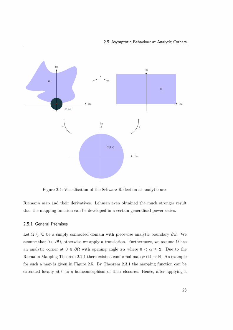
One of the main components for the proof is the result of Lehman that the mapping

function of a simply connected domain of the complex plain with an analytic corner

onto the upper half plain can be developed in a certain generalised power series. Based

on the result of Kaiser we get, as an application, the definability of Schwarz-Christoffel

maps, and working with circular polygons we get the definability of certain classes of

hypergeometric functions in this o-minimal structure, see Kaiser [8].

Let Ω ( C be a bounded, semianalytic domain which is simply connected. Then ∂Ω

has only finitely many singular boundary points. For such a singular boundary point

x ∈ ∂Ω there is a k ∈ N such that for all sufficiently small neighbourhoods V of x the set

Ω∩V has exactly k connected components having x as boundary point. We denote such

a connected component by C and the interior angle of ∂C at x by ^xC. Furthermore, let

Sing(∂Ω) := x ∈ ∂Ω | x is a singular boundary point of ∂Ω

and for x ∈ Sing(∂Ω)

^(Ω, x) := ^xC | C is a connected component of Ω ∩ V at x and x ∈ Sing(∂C).

Theorem 2.6.11 (T. Kaiser)

Suppose that ^(Ω, x) ⊂ π(R \Q) for all x ∈ Sing(∂Ω) then the Riemann map ϕ : Ω→ E

is definable in an o-minimal structure.

Proof: See Kaiser [8, Theorem 3.3 on p. 20 f.].

31

Chapter 3

Asymptotic Behaviour at Analytic Cusps

We consider a simply connected proper domain of the complex plane with piecewise

analytic boundary and an analytic cusp. Due to the Riemann Mapping Theorem, see

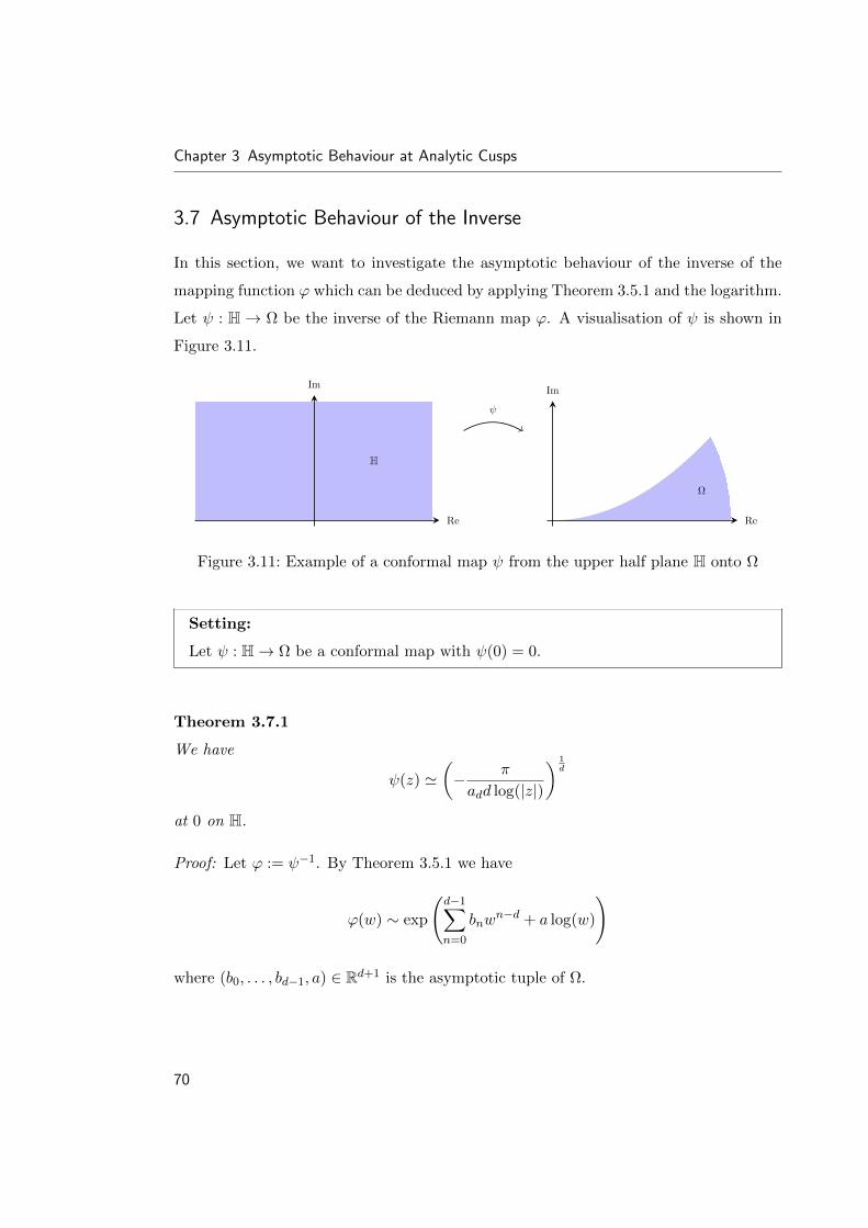
Theorem 2.2.1, we already know that there exists a conformal map from this domain

onto the upper half plane. An example for such a Riemann map is illustrated in Figure

3.1 below.

Re

Im

H

Re

Im

Figure 3.1: Example of a Riemann map from a simply connected domain with an analyticcusp onto the upper half plane

Due to Caratheodory, see Theorem 2.3.1, we can extend this Riemann map to the

boundary. We are especially interested in the behaviour of the mapping function at one

important point: the cusp. Under certain conditions on the domain, the so-called small

perturbation of angles, Kaiser already investigated the behaviour. After presenting the

results for this special case, we determine in this chapter the asymptotic behaviour in

33

Chapter 3 Asymptotic Behaviour at Analytic Cusps

the general case. Moreover, we show that after applying preliminary transformations

we can determine the asymptotic behaviour of such a Riemann map in the special case

that the analytic cusp is at 0 and that one of the boundary arcs in a neighbourhood of 0

coincides with the positive real axis. To investigate the behaviour, we give estimates for

the modulus and the argument of the Riemann map using a theorem of Warschawski.

Furthermore, we determine the asymptotic behaviour of its derivatives. By using these

results we can also investigate the behaviour of its inverse and, in addition, of the

derivatives of the inverse.

3.1 General Premises

Let Ω ( C be a simply connected domain which has an analytic cusp. We can assume

that the cusp is at 0, otherwise we apply a translation. We denote the boundary curves

by γ1 and γ2. There exists some ε > 0 such that γ1 and γ2 are analytic on B(0, ε) and

such that ∂Ω close to 0 is given by Γ1 ∪ Γ2 where Γ1 := γ1([0, ε[) and Γ2 := γ2([0, ε[).

Since Γ1 and Γ2 are regular by assumption we can assume that the parameterisations γ1

and γ2 are regular. Thus, we have γ1′(0)γ2

′(0) 6= 0. Furthermore, we may assume that,

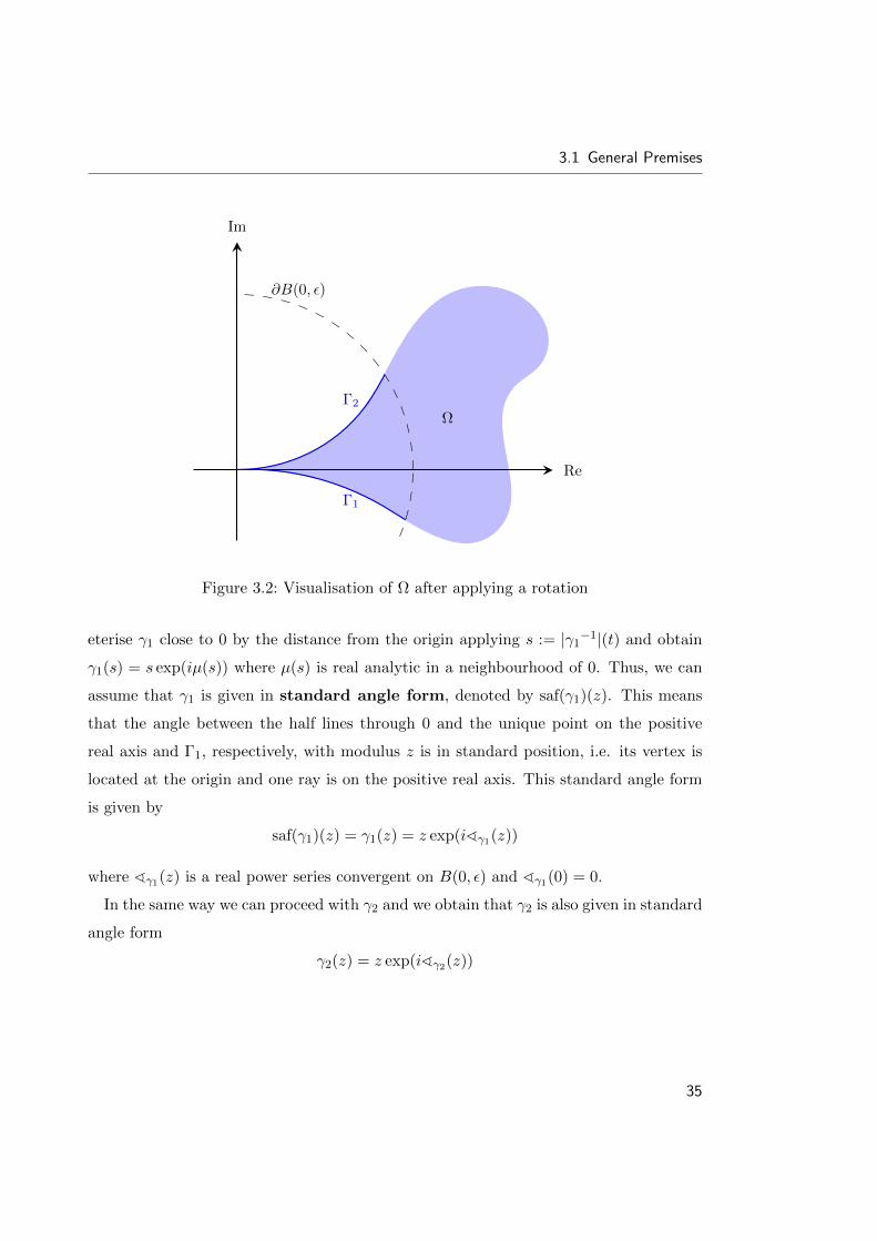
after applying a rotation, Ω is tangent to R≥0 at 0, i.e. γ1′(0) = γ2

′(0) > 0, as depicted

in Figure 3.2.

Now, if necessary, we shrink ε so we can write γ1(t) in polar coordinates as

γ1(t) = |γ1(t)| exp(iη1(t))

where

η1(t) := arg(γ1(t)) = arctan

(Im(γ1(t))

Re(γ1(t))

).

Since γ1(0) = 0 we have ord(Re(γ1(t))) ≥ 1 and ord(Im(γ1(t))) ≥ 1. Moreover,

we have γ1′(0) ∈ R>0 and thus, ord(Im(γ1(t))) ≥ 2. Since γ1

′(0) 6= 0 we obtain

ord(Re(γ1(t))) = 1. Hence, it follows that |γ1(t)| and η1(t) are real analytic on ] − ε, ε[and that ord(|γ1(t)|) = 1. Therefore, |γ1(t)| is locally invertible at 0. Now we can param-

34

3.1 General Premises

Re

Im

Ω

∂B(0, ε)

Γ2

Γ1

Figure 3.2: Visualisation of Ω after applying a rotation

eterise γ1 close to 0 by the distance from the origin applying s := |γ1−1|(t) and obtain

γ1(s) = s exp(iµ(s)) where µ(s) is real analytic in a neighbourhood of 0. Thus, we can

assume that γ1 is given in standard angle form, denoted by saf(γ1)(z). This means

that the angle between the half lines through 0 and the unique point on the positive

real axis and Γ1, respectively, with modulus z is in standard position, i.e. its vertex is

located at the origin and one ray is on the positive real axis. This standard angle form

is given by

saf(γ1)(z) = γ1(z) = z exp(i^γ1(z))

where ^γ1(z) is a real power series convergent on B(0, ε) and ^γ1(0) = 0.

In the same way we can proceed with γ2 and we obtain that γ2 is also given in standard

angle form

γ2(z) = z exp(i^γ2(z))

35

Chapter 3 Asymptotic Behaviour at Analytic Cusps

where ^γ2(z) is a real power series convergent on B(0, ε) and ^γ2(0) = 0. We set

^Ω(t) := ^γ2(t)− ^γ1(t).

Moreover, we assume that ^Ω(t) is positive for small positive t. Otherwise, we may

relabel γ1 and γ2. Geometrically, ^Ω(t) is the angle between the half lines through 0 and

the unique point on Γ1 and Γ2, respectively, with modulus t. A visualisation is depicted

in Figure 3.3.

Ω

∂B(0, ε)

∂B(0, t)

Re

Im

Γ2

Γ1

^γ1(t)

^γ2(t)

^Ω(t)

Figure 3.3: Visualisation of Ω, ^Ω, ^γ1 , and ^γ2

Definition 3.1.1

Let Ω and ^Ω(t) be as above. Let d := ord(^Ω(t)) ∈ N and let ad ∈ R>0 such that

^Ω(t) ' adtd. We call ot(Ω) := d the order of tangency of Ω and ct(Ω) := ad the

coefficient of tangency of Ω.

36

3.2 Small Perturbation of Angles

Let ϕ : Ω → H be a Riemann map. By Caratheodory, see Theorem 2.3.1, the given

mapping function can be extended continuously to the boundary and hence to the origin

with value in R. By applying a suitable translation we can assume without restriction

that ϕ(0) = 0. The arc Γ1 is mapped to the positive real axis and Γ2 is mapped to the

negative real axis.

Setting:

Let Ω ( C be a simply connected domain with an analytic cusp at 0 and let

ϕ : Ω→ H

be a Riemann map with ϕ(0) = 0.

3.2 Small Perturbation of Angles

As mentioned above, Kaiser investigates in [9] the asymptotic behaviour of the mapping

function at an analytic cusp in a special case, the so-called small perturbation of angles.

In this section, we present the basic definitions and his main result. In this article, he

also determines the asymptotic behaviour of its inverse and proves O-estimates for the

nth derivatives, where n ∈ N, of the mapping function and its inverse.

Definition 3.2.1

Let d := ot(Ω) and ad := ct(Ω). We say that Ω has small perturbation of angles if

the following is fulfilled:

(a) minord(^γ1(t)), ord(^γ2(t)) = d.

(b) ord(^Ω(t)− adtd) > 2d.

37

Chapter 3 Asymptotic Behaviour at Analytic Cusps

Example 3.2.2

Let d ∈ N and a ∈ R>0. For 0 < σ <(π2a

) 1d the domain

Ω := z ∈ C| 0 < |z| < σ, 0 < arg(z) < a|z|d

has small perturbation of angles. We have d := ot(Ω) and a := ct(Ω).

Theorem 3.2.3

Assume that Ω has small perturbation of angles. Then

ϕ(z) ∼ exp(− γ

zd

)

at 0 on Ω where d := ot(Ω) and γ := πot(Ω)ct(Ω)

.

Proof: We refer to Kaiser [9, Theorem 6 on p. 39 ff.].

3.3 Preliminary Transformation

Since γ1 is a regular parameterisation of Γ1 we have γ1′(0) 6= 0. Hence, there is some

δ > 0 such that γ1−1 exists on B(0, δ). Thus, we can apply the preliminary trans-

formation γ1−1 to Ω in a neighbourhood of 0 and thereby map the boundary arc Γ1

to the positive real axis. We denote γ1−1 (Ω ∩B(0, δ)) by Ωγ1 . The transformation

γ1(t) = t exp (i^γ1(t)) depends only on the shape of Ω at 0 and is therefore an invariant

of Ω. Hence, also γ1−1 is an invariant of Ω. For an illustration of the transformation

γ1−1 see Figure 3.4.

In the following we investigate the asymptotic behaviour of the Riemann map ϕ, as

introduced in Section 3.1, for the special case where Ω has already been transformed as

described above. For simplicity of notation we denote Ωγ1 by Ω for the rest of the work

and assume that the setting is as follows.

38

3.3 Preliminary Transformation

Setting:

The regular parameterisations of the boundary arcs of Ω in a neighbourhood of 0

are given by

γ1(t) = t and γ2(t) = t exp (i^Ω(t)) .

Thus, ^γ1(t) = 0 and ^Ω(t) = ^γ2(t). Furthermore, we assume that

^Ω(t) =

∞∑

n=d

antn

is a real power series with ad 6= 0 and d ∈ N.

Ω ∩B(0, δ)Re

Im

∂B(0, δ) γ−11

Ωγ1

Re

Im

Figure 3.4: Visualisation of the coordinate transformation γ1−1

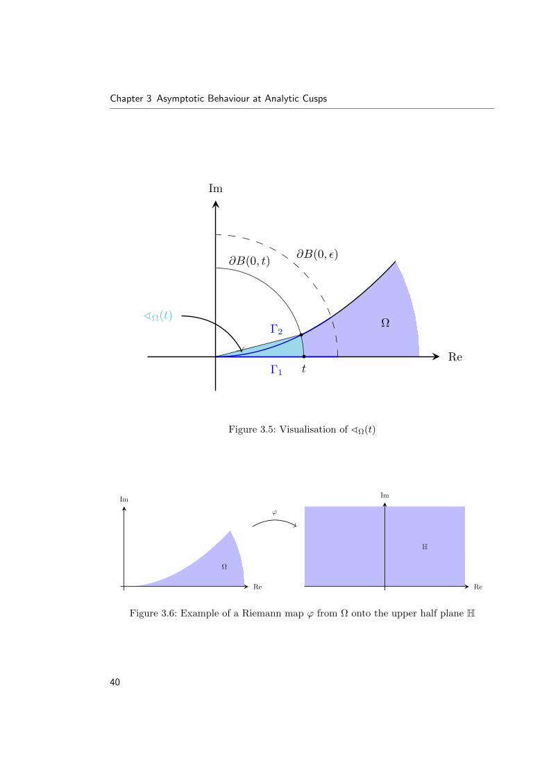
As already mentioned, ^Ω(t) is the angle between the half lines through 0 and the

unique point on Γ2 and on the positive real axis, respectively, with modulus t, see

Figure 3.5. In the following we determine the asymptotic behaviour of the Riemann

map ϕ : Ω→ H with Ω as stated above. An example for ϕ is depicted in Figure 3.6.

Note that by determining the asymptotic behaviour of ϕ in the above setting, we can

also derive the behaviour in the general case as introduced in Section 3.1.

39

Chapter 3 Asymptotic Behaviour at Analytic Cusps

Re

Im

Ω

∂B(0, ε)

Γ2

Γ1 t

∂B(0, t)

^Ω(t)

Figure 3.5: Visualisation of ^Ω(t)

Ω

Re

Im

ϕ

Re

Im

H

Figure 3.6: Example of a Riemann map ϕ from Ω onto the upper half plane H

40

3.4 Estimates for the Modulus and the Argument

3.4 Estimates for the Modulus and the Argument

In this section, we give estimates for the modulus and the argument of the mapping

function ϕ : Ω→ H. Therefore, we present a theorem of Warschawski who worked in a

more general setting than that of analytic arcs. This theorem, proven in [21], is on the

estimates for the modulus and the argument of a Riemann map from a simply connected

domain bounded by a Jordan arc onto the unit disk with center 1 in a neighbourhood

of a finite boundary point.

Let Θ ( C be a simply connected domain and let ∂Θ be a Jordan arc with 0 ∈ ∂Θ. We

denote the parameterisations of the boundary arcs of Θ at 0 by θ1 and θ2. Moreover, we

assume that these curves are given by θ1(t) = t exp (i^θ1(t)) and θ2(t) = t exp (i^θ2(t))

in a neighbourhood B(0, δ) with δ > 0. Analogously to Section 3.1, we set ^Θ(t) :=

^θ2(t)− ^θ1(t) and further let

θ(t) :=1

2(^θ1(t) + ^θ2(t)).

Suppose that ^θ1(t) and ^θ2(t) are absolutely continuous in any closed interval within

0 < t ≤ δ. Additionally, we assume that t^′θ1(t) and t^′θ2(t) approach the same limit,

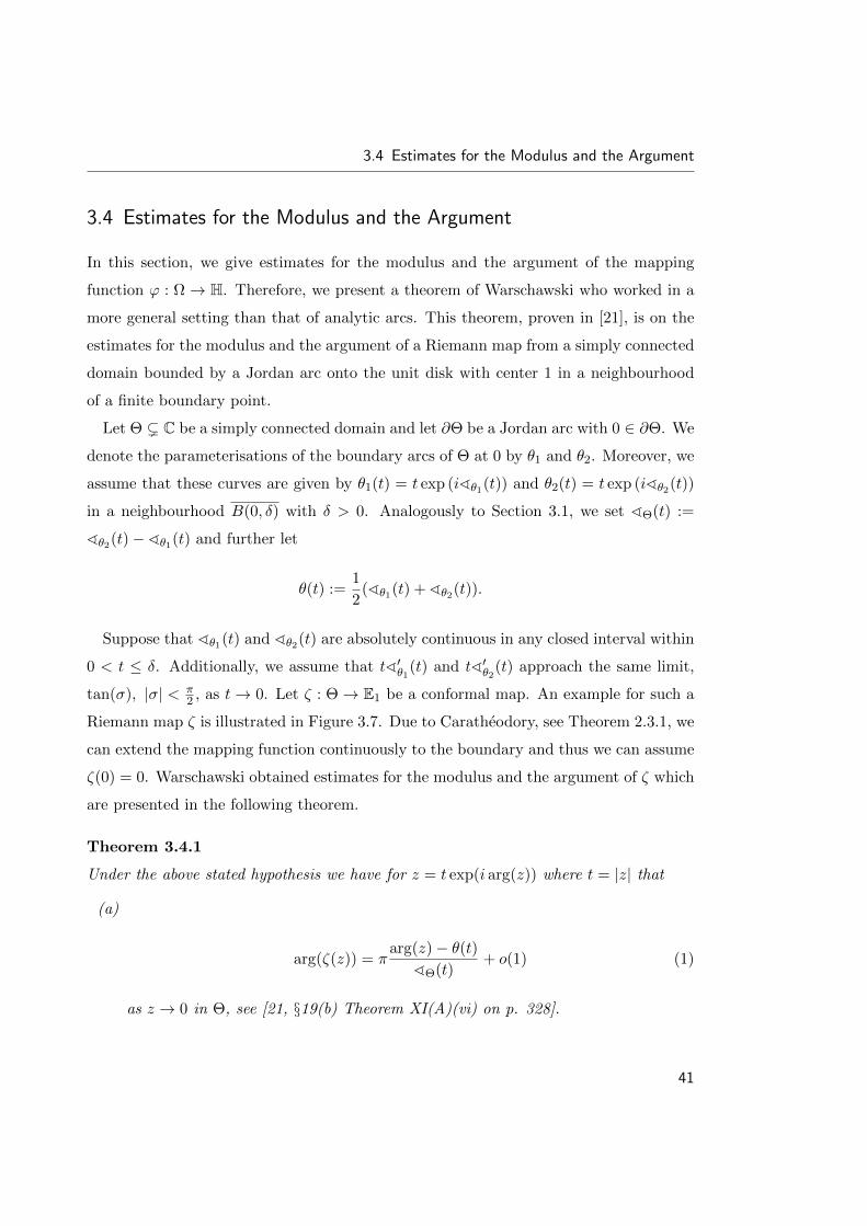
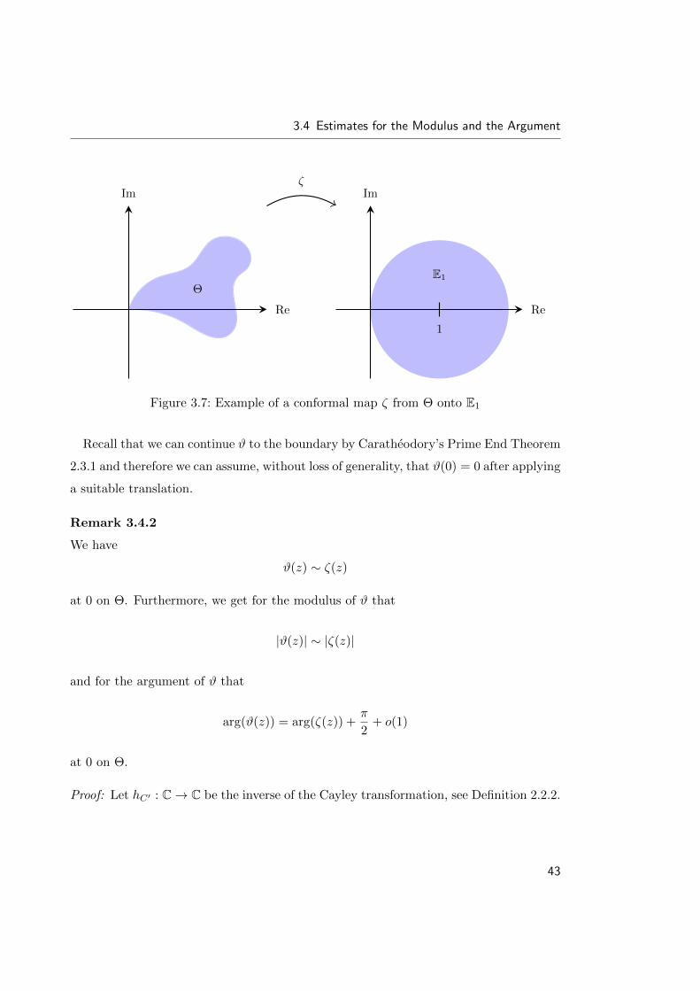
tan(σ), |σ| < π2 , as t→ 0. Let ζ : Θ→ E1 be a conformal map. An example for such a

Riemann map ζ is illustrated in Figure 3.7. Due to Caratheodory, see Theorem 2.3.1, we

can extend the mapping function continuously to the boundary and thus we can assume

ζ(0) = 0. Warschawski obtained estimates for the modulus and the argument of ζ which

are presented in the following theorem.

Theorem 3.4.1

Under the above stated hypothesis we have for z = t exp(i arg(z)) where t = |z| that

(a)

arg(ζ(z)) = πarg(z)− θ(t)

^Θ(t)+ o(1) (1)

as z → 0 in Θ, see [21, §19(b) Theorem XI(A)(vi) on p. 328].

41

Chapter 3 Asymptotic Behaviour at Analytic Cusps

(b) If t^′θ1(t) and t^′θ2(t) are continuous for 0 ≤ t ≤ δ and the integrals

δ∫

0

^′′θ1(t)dt,

δ∫

0

^′′θ2(t)dt, and

δ∫

0

(^′Θ(t))2

^Θ(t)dt

converge then there exists some c > 0 such that

|ζ(z)| = c exp

−π

δ∫

t

1 + (rθ′(r))2

r^Θ(r)dr + π

arg(z)− θ(t)^Θ(t)

tan(σ) + o(1)

(2)

as z → 0 in Θ. See [21, §19(b) Theorem XI(B) on p. 328]. If in addition the

integralsδ∫

0

t

^Θ(t)(^′θ1(t))2dt and

δ∫

0

t

^Θ(t)(^′θ2(t))2dt

converge, then (2) reduces to

|ζ(z)| = c exp

−π

δ∫

t

dr

r^Θ(r)+ o(1)

as z → 0 in Θ, see [21, §19(c) Remark on p. 328].

Proof: As stated in Warschwaski [21, p. 327 f.], (a) follows from [21, Theorem X on p.

315 and Corollary 1 on p. 323] and (b) follows from [21, Corollary of Theorem VIII on

p. 313 and Corollary of Theorem IV on p. 296].

In the following, it is our aim to adapt his result to our case where we map onto the

upper half plane instead of mapping onto E1. First, we give a remark on the asymptotic

behaviour of a Riemann map ϑ : Θ→ H and obtain estimates for the modulus and the

argument of ϑ in terms of ζ, see Remark 3.4.2. Second, we adapt the above theorem to

the situation where we map Ω, having an analytic cusp at 0, to the upper half plane,

see Corollary 3.4.6.

42

3.4 Estimates for the Modulus and the Argument

Θ

Re

Imζ

Re

Im

E1

1

Figure 3.7: Example of a conformal map ζ from Θ onto E1

Recall that we can continue ϑ to the boundary by Caratheodory’s Prime End Theorem

2.3.1 and therefore we can assume, without loss of generality, that ϑ(0) = 0 after applying

a suitable translation.

Remark 3.4.2

We have

ϑ(z) ∼ ζ(z)

at 0 on Θ. Furthermore, we get for the modulus of ϑ that

|ϑ(z)| ∼ |ζ(z)|

and for the argument of ϑ that

arg(ϑ(z)) = arg(ζ(z)) +π

2+ o(1)

at 0 on Θ.

Proof: Let hC′ : C→ C be the inverse of the Cayley transformation, see Definition 2.2.2.

43

Chapter 3 Asymptotic Behaviour at Analytic Cusps

Then we have hC′(E) = H. Furthermore, let g : C → C with g(z) = z − 1. Thus,

g(E1) = E. Then

f := hC′ g : E1 → H

is given by

f(z) = iz

2− z . (3.1)

Since the power series of f around 0 is given by

∞∑

n=0

anzn

where an = f (n)(0)n! we obtain with ζ : Θ→ E1 that

ϑ = f ζ : Θ→ H, ϑ(z) =∞∑

n=0

an(ζ(z))n.

Since a0 = f(0)0! = 0 and

a1 =f ′(0)

1!= h′C′(−1) =

i

26= 0,

we get

ϑ(z) ∼ ζ(z).

Therefore, we obtain

|ϑ(z)| ∼ |ζ(z)|.

Moreover, we have with (3.1)

arg (ϑ(z)) = arg

(i

ζ(z)

2− ζ(z)

)

2+ arg(ζ(z))− arg(2− ζ(z)).

44

3.4 Estimates for the Modulus and the Argument

Since

limz→0

arg (2− ζ(z)) = 0

we get

arg(ϑ(z)) = arg(ζ(z)) +π

2+ o(1).

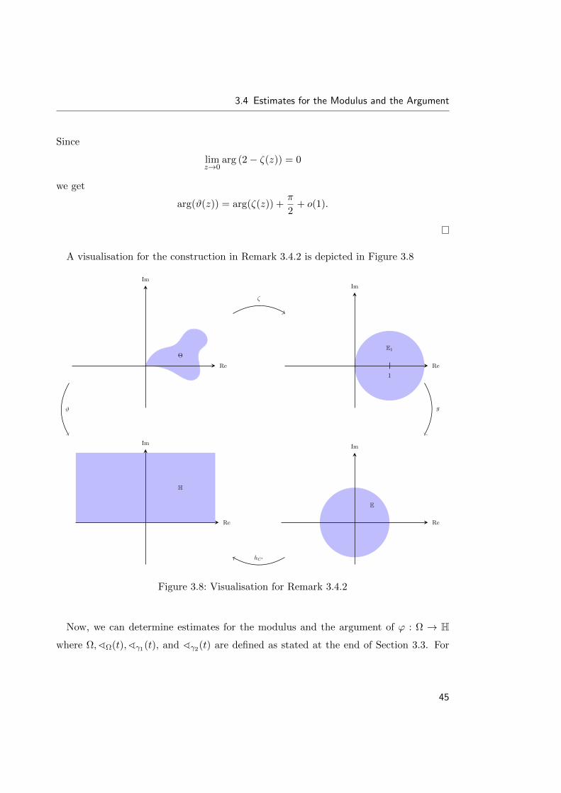
A visualisation for the construction in Remark 3.4.2 is depicted in Figure 3.8

Θ

Re

Im

ζ

Re

Im

1

E1

g

Re

Im

E

hC′

Re

Im

H

ϑ

Figure 3.8: Visualisation for Remark 3.4.2

Now, we can determine estimates for the modulus and the argument of ϕ : Ω → H

where Ω,^Ω(t),^γ1(t), and ^γ2(t) are defined as stated at the end of Section 3.3. For

45

Chapter 3 Asymptotic Behaviour at Analytic Cusps

this proof we need the multiplicative inverse of a Laurent series and thus we recall below

the computation rule for multiplicative inversion of a convergent power series, refer also

to Freitag and Busam [6, p. 118].

Remark 3.4.3

Let

f(z) =∞∑

n=0

anzn

be a convergent power series with a0 6= 0. Then there exists some ε > 0 such that

f(z) 6= 0 for all z in B(0, ε). Let g(z) = 1f(z) then g(z) is analytic on B(0, ε) and thus

representable as a power series

g(z) =

∞∑

n=0

bnzn.

The coefficients of the multiplicative inverse power series g(z) of f(z) can be computed

as follows. Since f(z)g(z) = 1 we obtain by the Cauchy product formula

n∑

k=0

akbn−k =

1 for n = 0,

0 for n 6= 0.

This system of equations can be recursively solved with respect to n.

Example 3.4.4

We want to determine the coefficients cn of the Laurent series

∞∑

n=0

cntn−d =

1

^Ω(t)

where d is the order of tangency. Since

^Ω(t) =

∞∑

n=d

antn = td

∞∑

n=0

ad+ntn

46

3.4 Estimates for the Modulus and the Argument

we obtain ∞∑

n=0

cntn−d =

1

td

∞∑

n=0

cntn =

1

td1

∞∑n=0

ad+ntn.

Thus,∞∑n=0

cntn is the multiplicative inverse of

∞∑

n=0

ad+ntn

where the coefficient of tangency ad 6= 0, i.e.

( ∞∑

n=0

cntn

)( ∞∑

n=0

ad+ntn

)= 1.

Therefore, we obtain

n∑

k=0

ckad+n−k =

1 for n = 0,

0 for n 6= 0.

Hence, we can determine the coefficients cn in the following way:

cn =

1ad

for n = 0,

−n−1∑k=0

ckad+n−kad

for n 6= 0.

By solving these equations we obtain

c0 =1

ad,

c1 = −0∑

k=0

ckad+1−kad

= −c0ad+1

ad= −ad+1

a2d

,

c2 = −1∑

k=0

ckad+2−kad

= −c0ad+2

ad− c1

ad+1

ad= −ad+2

a2d

−(−ad+1

a2d

)ad+1

ad=a2d+1

a3d

− ad+2

a2d

. . .

47

Chapter 3 Asymptotic Behaviour at Analytic Cusps

Definition 3.4.5

Let cn be the coefficients of the Laurent series

∞∑

n=0

cntn−d =

1

^Ω(t)

where d is the order of tangency. Moreover, we set for 0 ≤ n ≤ d− 1

bn :=πcnn− d and a := πcd.

We call the tuple (b0, . . . , bd−1, a) ∈ Rd+1 the asymptotic tuple of Ω.

The elements of the asymptotic tuple (b0, . . . , bd−1, a) ∈ Rd+1 of Ω in Definition 3.4.5

are geometric invariants depending on the shape of the domain Ω at the cusp since they

can be computed by using ^Ω(t), the real power series which describes the cusp. For the

rest of the work all statements regarding the asymptotic behaviour of mapping functions

focus on the case that z → 0. The next result can be shown by applying Theorem 3.4.1

of Warschawski and Remark 3.4.2.

Corollary 3.4.6

We have

(a)

|ϕ(z)| = c exp

(|z|−d

d−1∑

n=0

bn|z|n + a log |z|+ o(1)

)

where c ∈ R>0 is a constant and (b0, . . . , bd−1, a) is the asymptotic tuple of Ω.

(b)

arg(ϕ(z)) = π arg(z)|z|−d(

d∑

n=0

cn|z|n)

+ o(1).

Proof:

Case 1: Let d > 1.

First of all, we have to check the conditions of Theorem 3.4.1. Since ^γ1(t) = 0 and

48

3.4 Estimates for the Modulus and the Argument

^γ2(t) = ^Ω(t) ' adtd it follows that ^′′γ1(t) = 0 and ^′′γ2(t) = O(td−2). Therefore, the

integrals

δ∫

0

^′′γ1(t)dt and

δ∫

0

^′′γ2(t)dt (3.2)

converge for small δ > 0. Moreover, we have (^′Ω(t))2 ' a2dd

2t2d−2 and thus

(^′Ω(t))2

^Ω(t)' add2td−2.

Therefore,(^′Ω(t))2

^Ω(t)= O(td−2)

and, as a consequence, the integral

δ∫

0

(^′Ω(t))2

^Ω(t)dt (3.3)

converges for small δ > 0. In addition, the integrals

δ∫

0

t

^Ω(t)(^′γ1(t))2dt and

δ∫

0

t

^Ω(t)(^′Ω(t))2dt (3.4)

converge for small δ > 0 since

t

^Ω(t)(^′γ1(t))2 = 0 and

t

^Ω(t)(^′Ω(t))2 ' add2td−1

and thust

^Ω(t)(^′Ω(t))2 = O(td−1).

By using (3.2), (3.3), and (3.4) we get from Theorem 3.4.1 and Remark 3.4.2 the following

49

Chapter 3 Asymptotic Behaviour at Analytic Cusps

estimate for the modulus of ϕ

|ϕ(z)| = p1 exp

−π

δ∫

t

1

r^Ω(r)dr + o(1)

(3.5)

for some constant p1 > 0 with t = |z|. By computing the integral in (3.5) we obtain for

t→ 0 the desired estimate. For this calculation we set

h(t) := −πδ∫

t

1

r^Ω(r)dr

and1

^Ω(t):=

∞∑

n=0

cntn−d.

The coefficients cn can be determined as in Example 3.4.4. Hence, we get

h(t) = −πδ∫

t

1

r^Ω(r)dr

= −πδ∫

t

∞∑

n=0

cnrn−(d+1)dr

= −π

δ∫

t

d−1∑

n=0

cnrn−(d+1)dr +

δ∫

t

cdrd−(d+1)dr +

δ∫

t

∞∑

n=d+1

cnrn−(d+1)dr

= −π(d−1∑

n=0

cn

[1

n− drn−d]δ

t

+ [cd log(r)]δt +∞∑

n=d+1

cn

[1

n− drn−d]δ

t

)

= −π(p2 −

d−1∑

n=0

cnn− dt

n−d − cd log(t)−∞∑

n=d+1

cnn− dt

n−d

)

with a constant p2 ∈ R. Since

limt→0

∞∑

n=d+1

cnn− dt

n−d = 0

50

3.4 Estimates for the Modulus and the Argument

it follows that

h(t) = −πp2 + π

d−1∑

n=0

cnn− dt

n−d + πcd log(t) + o(1).

Therefore, we obtain for |z| = t that

|ϕ(z)| = p1 exp (h(t) + o(1))

= p1 exp

(−πp2 + π

d−1∑

n=0

cnn− dt

n−d + πcd log(t) + o(1)

)

= p3 exp

(πd−1∑

n=0

cnn− dt

n−d + πcd log(t) + o(1)

)

where p3 := p1 exp(−πp2).

Now we prove the estimate for the argument of ϕ. As in our case θ(t) = 12^Ω(t) it

follows with Theorem 3.4.1 and Remark 3.4.2 that

arg(ϕ(z)) = πarg(z)

^Ω(t)− π ^Ω(t)

2^Ω(t)+π

2+ o(1)

= πarg(z)

^Ω(t)+ o(1)

= π arg(z)

∞∑

n=0

cntn−d + o(1).

Moreover, we have

limt→0

∞∑

n=d+1

cntn−d = 0

and therefore we obtain

arg(ϕ(z)) = π arg(z)

d∑

n=0

cntn−d + o(1).

Case 2: Let d = 1.

We apply the transformation ω : C → C, ω(z) =√z to Ω and we set Ω := ω(Ω).

51

Chapter 3 Asymptotic Behaviour at Analytic Cusps

The boundary arcs of the domain Ω in a neighbourhood of 0 are given by the following

parameterisations

γ1(t) =√t and γ2(t) =

√t exp

(i1

2^Ω(t)

).

Substituting s :=√t we obtain the parametric representation for the boundary arcs of Ω

of the form

γ1(s) = s and γ2(s) = s exp(i^Ω

(s))

where ^Ω

(s) = 12^Ω(s2). Therefore,

(s) =

∞∑

n=d

ansn

where d = 2. Let ϕ : Ω → H. Since ^Ω

fulfils the condition from Case 1, we obtain

the following estimates for the modulus and the argument of the mapping function

ϕ(ω(z)) = ϕ : Ω→ H:

|ϕ(z)| = |ϕ(ω(z))|

= p3 exp

π

d−1∑

n=0

cn

n− dsn−d + πc

dlog(s) + o(1)

= p3 exp

1∑

n=0

cnn− 2

sn−2 + πc2 log(s) + o(1)

)

for some constant p3 > 0 and

arg(ϕ(z)) = arg(ϕ(ω(z)))

= π arg(ω(z))d∑

n=0

cnsn−d + o(1)

= π arg(ω(z))

2∑

n=0

cnsn−2 + o(1)

52

3.4 Estimates for the Modulus and the Argument

where cn are the coefficients of the Laurent series

∞∑

n=0

cnsn−(d+1) =

1

s^Ω

(s).

As in Case 1, the coefficients cn can be determined as in Example 3.4.4. Since

(s) =1

2^Ω(s2) =

a1

2s2 +

a2

2s4 +

a3

2s6 +O

(s8)

we are able to compute the first three coefficients, namely

c0 =2

a1= 2c0, c1 = 0 and c2 = −2a2

a21

= 2c1. (3.6)

Using these results and substituting s =√t back, we end up with

|ϕ(z)| = p3 exp

(− c0

2

√t−2 − c1

√t−1)

+ πc2 log(√t) + o(1)

)

(3.6)= p3 exp

(−πc0t

−1 + πc1 log(t)) + o(1))

and since arg(ω(z)) = arg (√z) = 1

2 arg(z) we have

arg(ϕ(z)) =π

2arg(z)

2∑

n=0

cn√tn−2

+ o(1)

2arg(z)

(c0

√t−2

+ c1

√t−1

+ c2

)+ o(1)

(3.6)=

π

2arg(z)

(2c0t

−1 + 2c1

)+ o(1)

= π arg(z)(c0t−1 + c1

)+ o(1).

In summary, we get

|ϕ(z)| =

p3 exp(−πc0t

−1 + πc1 log(t) + o(1))

for d = 1,

p3 exp

(πd−1∑n=0

cnn−d t

n−d + πcd log(t) + o(1)

)for d > 1

53

Chapter 3 Asymptotic Behaviour at Analytic Cusps

and

arg(ϕ(z)) =

π arg(z)(c0t−1 + c1

)+ o(1) for d = 1,

π arg(z)d∑

n=0cnt

n−d + o(1) for d > 1

which simplifies to

|ϕ(z)| = c exp

(t−dπ

d−1∑

n=0

cnn− dt

n + πcd log(t) + o(1)

)

for d ∈ N and some constant c ∈ R>0 and

arg(ϕ(z)) = π arg(z)t−dd∑

n=0

cntn + o(1)

for d ∈ N, respectively.

3.5 Asymptotic Behaviour of the Riemann map

By using Corollary 3.4.6 and Lemma 2.1.20 we can immediately determine the asymp-

totic behaviour of the mapping function ϕ.

Theorem 3.5.1

We have

ϕ(z) ∼ za exp

(b0zd

+b1zd−1

+ · · ·+ bd−1

z

)

at 0 on Ω where (b0, . . . , bd−1, a) is the asymptotic tuple of Ω.

Proof: Let |z| = t. We set

h(t) :=d−1∑

n=0

bntn−d + a log(t) and g(z) := arg(ϕ(z)).

54

3.5 Asymptotic Behaviour of the Riemann map

We have by Corollary 3.4.6

log (ϕ(z)) = log (|ϕ(z)| exp(ig(z)))

= log (c exp(h(t) + o(1)) exp(ig(z)))

= log(c) + log (exp(h(t) + o(1))) + log (exp(ig(z)))

= log(c) + h(t) + ig(z) + o(1) (3.7)

where c ∈ R>0 is a constant. By fixing

H(z) :=d−1∑

n=0

bnzn−d + a log(z)

it follows that

Re(H(z)) =

d−1∑

n=0

bntn−d cos

((n− d) arg(z)

)+ a log(t)

and

Im(H(z)) =d−1∑

n=0

bntn−d sin

((n− d) arg(z)

)+ a arg(z).

Next, we show that

H(z) = h(t) + ig(z) + o(1). (3.8)

By the power series expansion of cosine we see that

cos((n− d) arg(z)) = 1 +O((arg(z))2). (3.9)

Since ^Ω(t) = adtd +O(td+1) on Ω we have 0 ≤ arg(z) ≤ adtd +O(td+1) and thus

0 ≤ (arg(z))2 ≤ a2dt

2d +O(t2d+1) (3.10)

55

Chapter 3 Asymptotic Behaviour at Analytic Cusps

for z ∈ Ω close to 0. By Definition 3.4.5 we have bn = πcnn−d and a = cdπ. Hence, by using

the estimates above we obtain

limz→0

(Re(H(z))− h(t))

= limz→0

(d−1∑

n=0

bntn−d (cos

((n− d) arg(z)

)− 1)

+ πcd log(t)− πcd log(t)

)

(3.9)= lim

z→0

d−1∑

n=0

bntn−d (1 +O

((arg(z))2

)− 1)

= limz→0

d−1∑

n=0

bntn−d (O

((arg(z))2

))

(3.10)= lim

z→0

d−1∑

n=0

bntn−d

(a2dt

2d +O(t2d+1

))

= 0.

Thus, it follows that

Re(H(z))− h(t) = o(1). (3.11)

By the power series expansion of sine we get

sin((n− d) arg(z)) = (n− d) arg(z) +O((arg(z))3) (3.12)

and moreover we have on Ω

0 ≤ (arg(z))3 ≤ a3dt

3d +O(t3d+1). (3.13)

56

3.5 Asymptotic Behaviour of the Riemann map

Using these estimates we get

limz→0

(Im(H(z))− g(z))

= limz→0

(d−1∑

n=0

bntn−d sin

((n− d) arg(z)

)+ πcd arg(z)− arg(ϕ(z))

)

3.4.6= lim

z→0

(d−1∑

n=0

bntn−d sin

((n− d) arg(z)

)+ πcd arg(z)− π arg(z)

d∑

n=0

cntn−d + o(1)

)

(3.12)= lim

z→0

(d−1∑

n=0

πcnn− dt

n−d ((n− d) arg(z) +O((arg(z))3

))+ πcd arg(z)

−π arg(z)

d−1∑

n=0

cntn−d − πcd arg(z) + o(1)

)

= limz→0

(d−1∑

n=0

πcntn−d (arg(z) +O

((arg(z))3

)− arg(z)

)+ o(1)

)

= limz→0

(d−1∑

n=0

πcntn−d (O

((arg(z))3

))+ o(1)

)

(3.13)= lim

z→0

(d−1∑

n=0

πcntn−d(a3

dt3d +O

(t3d+1)

)+ o(1)

)

= 0.

Hence, we have shown that

Im(H(z))− g(z) = o(1). (3.14)

Therefore, by (3.11) and (3.14) we get (3.8) and thus we obtain

log(ϕ(z))(3.7)= log(c) + h(t) + ig(z) + o(1) = log(c) +H(z).

Applying Lemma 2.1.20 shows

ϕ(z) ' exp(log(c) +H(z)) ∼ exp(H(z)). (3.15)

57

Chapter 3 Asymptotic Behaviour at Analytic Cusps

Thus, it follows that

ϕ(z) ∼ za exp

(b0zd

+ · · ·+ bd−1

z

)

at 0 on Ω.

Now we are able to determine the asymptotic behaviour of an example mentioned by

Kaiser in [9, Remark 8(i)]. This was not possible before since the domain introduced in

this example has not small perturbation of angles.

Example 3.5.2

Let

Ω :=

z ∈ C | 0 < |z| < 1

2, 0 < arg(z) < |z| − |z|2

.

Then Ω is a simply connected domain with an analytic cusp at 0 which is tangent to

R≥0 as depicted in Figure 3.9.

12

Ω

Re

Im

Figure 3.9: Visualisation of Ω

The boundary curves at 0 are given by γ1(t) = t and γ2(t) = t exp(i(t − t2)). Let

ϕ : Ω → H be a conformal map with ϕ(0) = 0. Since ^Ω(t) = t − t2 we get from

Theorem 3.5.1 with ot(Ω) = d = 1 that

ϕ(z) ∼ za exp(b0z−1)

58

3.5 Asymptotic Behaviour of the Riemann map

where b0 = πc00−1 = −πc0 and a = πc1. We have to compute c0 and c1. Since ct(Ω) =

a1 = 1 and a2 = −1 we obtain from Example 3.4.4 that c0 = 1a1

= 1 and c1 = −c0a2a1

= 1

and therefore we get b0 = −π and a = π. Finally, it follows that

ϕ(z) ∼ zπ exp(−πz

)

at 0 on Ω.

We are now interested in a characterisation for the situation that the logarithmic

term of

exp

(b0zd

+b1zd−1

+ · · ·+ bd−1

z+ a log(z)

)∼ ϕ(z)

vanishes, i.e. a = 0. The following remark shows that the disappearance of the logarith-

mic term only depends on a finite number of coefficients of the power series ^Ω(t).

Remark 3.5.3

If ad+1 = . . . = a2d = 0 we have

ϕ(z) ∼ exp

(− π

addzd

)

at 0 on Ω.

Proof: Using Theorem 3.5.1 we see that

ϕ(z) ∼ za exp

(b0zd

+b1zd−1

+ · · ·+ bd−1

z

)

where (b0, . . . , bd−1, a) ∈ Rd+1 is the asymptotic tuple of Ω with bn = πcnn−d and a = πcd

as in Definition 3.4.5. From Example 3.4.4 we obtain

cn =

1ad

for n = 0,

−n−1∑k=0

ckad+n−kad

for n 6= 0

59

Chapter 3 Asymptotic Behaviour at Analytic Cusps

and since ad+1 = . . . = a2d = 0 we have ad+n−k = 0 for 0 < n ≤ d. Thus, we get

cn =

1ad

for n = 0,

0 for 0 < n ≤ d.

Therefore, b0 = − πadd

, bn = 0 for n ∈ 1, . . . , d− 1, and a = 0 since cd = 0. Hence, the

claim is proven.

The result of this special case coincides with the result of Theorem 3.2.3. Thus, the

logarithmic term vanishes if Ω has small perturbation of angles.

3.6 Asymptotic Behaviour of the Derivatives

For the following, we are interested in the asymptotic behaviour of the derivatives of ϕ.

We are going to prove that for n ∈ N0

ϕ(n)(z) ∼ za−n(d+1) exp

(b0zd

+ · · ·+ bd−1

z

)

at 0 on Ω by using the asymptotic behaviour of ϕ, determined in Theorem 3.5.1, and

the following proposition on the behaviour of the derivatives of

za exp

(b0zd

+ · · ·+ bd−1

z

).

Proposition 3.6.1

Let F : C∗ → C be given by

F (z) = za exp

(b0zd

+ · · ·+ bd−1

z

)

where (b0, . . . , bd−1, a) is the asymptotic tuple of Ω. Then we have for n ∈ N at 0 on C∗

that

F (n)(z) ∼ F (z)z−n(d+1).

60

3.6 Asymptotic Behaviour of the Derivatives

Proof: Let

H(z) :=d−1∑

k=0

bkzk−d + a log(z).

By the formula of Faa di Bruno (see Roman [19]) for the derivatives of the composition

of two functions and the fact that exp(n)(z) = exp(z) for n ∈ N we see that

F (n)(z) =dn

dzn(exp(H(z)))

=∑

(k1,...,kn)∈Tn

n!

k1! · . . . · kn!exp(k1+...+kn)(H(z))

n∏

m=1

(1

m!

dm

dzmH(z)

)km

=∑

(k1,...,kn)∈Tn

n!

k1! · . . . · kn!exp(H(z))

n∏

m=1

(1

m!

dm

dzmH(z)

)km

where Tn is the set of all n-tupel (k1, . . . , kn) with ki ∈ N0 for i ∈ 1, . . . , n and 1k1 +

2k2 + . . .+ nkn = n. Since

1

m!

dm

dzmH(z) =

1

m!

dm

dzm

(d−1∑

k=0

bkzk−d + a log(z)

)

=1

m!b0(−d)(−d− 1) · . . . · (−d− (m− 1))z−d−m + . . .

+1

m!bd−1(−1)(−2) · . . . · (−1− (m− 1))z−1−m

+1

m!a(−1)(−2) · . . . · (−(m− 1))z−m

∼ z−(d+m)

for m ∈ N and 1k1 + . . .+ nkn = n we have

n∏

m=1

(1

m!

dm

dzmH(z)

)km∼

n∏

m=1

z−(d+m)km

= z−(d+1)k1 · . . . · z−(d+n)kn

= z−(k1+...+kn)d−(1k1+...+nkn)

= z−(k1+...+kn)d−n. (3.16)

61

Chapter 3 Asymptotic Behaviour at Analytic Cusps

Note that k1 + . . .+ kn ∈ 1, . . . , n and k1 + . . .+ kn = n if and only if k1 = n. Thus,

it follows that

F (n)(z) =∑

(k1,...,kn)∈Tn

n!

k1! · . . . · kn!exp(H(z))

n∏

m=1

(1

m!

dm

dzmH(z)

)km

= exp(H(z))∑

(k1,...,kn)∈Tn

n!

k1! · . . . · kn!

n∏

m=1

(1

m!

dm

dzmH(z)

)km

∼ exp(H(z))∑

(k1,...,kn)∈Tn

n!

k1! · . . . · kn!z−(k1+...+kn)d−n

∼ exp(H(z))z−n(d+1)

= F (z)z−n(d+1).

As already mentioned above, there is some δ > 0 such that γ2−1 exists on B(0, δ). Let

Ωγ2 := γ2−1(Ω ∩B(0, δ)). Then we have the following lemma.

Lemma 3.6.2

We have for Ωγ2 as introduced above that

ot(^Ωγ2

(t))

= ot (^Ω(t)) .

Proof: By the general premises we have that the parameterisations of the boundary arcs

of Ω are given by γ1(z) = z and γ2(z) = z exp (i^Ω(z)) in a neighbourhood of 0 and

that ot (^Ω(t)) = d. Therefore, the parameterisations of the boundary arcs of Ωγ2 are

given by

γ1(z) = γ2−1(z) and γ2(z) = z

in a neighbourhood of 0. The standard angle form of γ1(z) is given by saf(γ1)(z) =

z exp(i^Ωγ2

(z)). By the power series expansion of the inverse we obtain

γ2−1(t) = t− ictd+1 +O

(td+2

)

62

3.6 Asymptotic Behaviour of the Derivatives

for some constant c ∈ R∗ and thus we read off that

ord(∣∣γ2

−1(t)∣∣) = 1,

ord(Re(γ2−1(t)

))= 1, (3.17)

ord(Im(γ2−1(t)

))= d+ 1.

We have

γ2−1(t) = ω1(t) exp (iω2(t))

where

ω1(t) =∣∣γ2−1(t)

∣∣ and ω(t) := arctan

(Im(γ2−1(t)

)

Re (γ2−1(t))

).

With (3.17) we see that ord(ω−1

1 (t))

= 1 and ord (ω2(t)) = d. Since ^Ωγ2(t) =

ω2

(ω−1

1 (t))

we have ord(^Ωγ2

(t))

= d = ord (^Ω(t)) and the lemma holds.

Theorem 3.6.3

Let n ∈ N0. Then

ϕ(n)(z) ∼ ϕ(z)z−n(d+1) ∼ za−n(d+1) exp

(b0zd

+ · · ·+ bd−1

z

)

at 0 on Ω where (b0, . . . , bd−1, a) is the asymptotic tuple of Ω.

Proof: We set

H(z) :=d−1∑

k=0

bkzk−d + a log(z)

and

F (z) := exp(H(z)).

By the preliminaries the boundary arcs of Ω are given by Γ1 and Γ2 in some neighbour-

hood of 0 with the regular parameterisations γ1(z) = z and γ2(z) = z exp(i^Ω(z)). Since

γ2′(0) = 1 we see that γ2 is locally invertible. Let r, s ∈ R with 0 < s < r such that

γ2(z) is injective on B(0, r) and that B(0, s) ⊂ γ2(B(0, r)). By the Schwarz Reflection

63

Chapter 3 Asymptotic Behaviour at Analytic Cusps

Principle via conjugation, see Theorem 2.4.1, we can continue ϕ across the analytic arc

Γ1. The reflection of Ω across Γ1 is given by

Ω1 := z ∈ C| z ∈ Ω.

By the Schwarz Reflection at analytic arcs, see Theorem 2.4.3, there exists an holomor-

phic extension of ϕ across Γ2. We denote the reflection of Ω across the boundary arc Γ2

by

Ω2 := z ∈ C| z ∈ B(0, s) and γ2(γ2−1(z)) ∈ Ω.

Furthermore, let

Ω := (Ω ∪ Γ1 ∪ Γ2 ∪ Ω1 ∪ Ω2) ∩B(0, s).

A visualisation of Ω is depicted in Figure 3.10.

Re

Im

Γ2

Γ1

Ω

Ω

Figure 3.10: Visualisation of Ω

Thus, there exists an holomorphic extension of ϕ, which we denote by Φ : Ω→ C, in

64

3.6 Asymptotic Behaviour of the Derivatives

some neighbourhood of 0. This extension is given by

Φ(z) =

ϕ(z) for z ∈ Ω ∪ Γ1 ∪ Γ2,

ϕ(z) for z ∈ Ω1,

ϕ(γ2

(γ2−1(z)

))for z ∈ Ω2.

Since F is holomorphic on C−, it also has an holomorphic extension to Ω after shrinking

r and s if necessary. We now prove the following claim on the asymptotic behaviour of Φ.

Claim 1: Φ(z) ∼ F (z) at 0 on Ω.

Proof of Claim 1: By Theorem 3.5.1 we have ϕ(z) ∼ F (z) at 0 on Ω ∪ Γ1 ∪ Γ2. Since

F (z) = F (z)

for z ∈ C− we have for Φ that

Φ(z) = ϕ(z) ∼ F (z) (3.18)

at 0 on Ω1. It remains to be shown that Φ(z) ∼ F (z) at 0 on Ω2. From γ2(0) =

γ2−1(0) = 0 we get at 0 on Ω2 that

ϕ(γ2

(γ2−1(z)

))∼ F

(γ2

(γ2−1(z)

)). (3.19)

Therefore, we have to show that

F(γ2

(γ2−1(z)

))∼ F (z)

at 0 on Ω2. We have

F (γ2(z)) = exp

(d−1∑

k=0

bk (γ2(z))k−d + a log (γ2(z))

).

65

Chapter 3 Asymptotic Behaviour at Analytic Cusps

Since γ2(z) = z exp (i^Ω(z)) we see by the power series expansion of the exponential

function that

(γ2(z))k−d = zk−d +O(zk)

for k ∈ 0, . . . , d− 1. Hence, we obtain

F (γ2(z)) = exp

(d−1∑

k=0

bk

(zk−d +O

(zk))

+ a log (z exp(i^Ω(z)))

)

= exp

(d−1∑

k=0

bkzk−d +

d−1∑

k=0

bkO(zk)

+ a log(z) + log (exp(ia^Ω(z))) + 2πil(z)

)

= exp

(d−1∑

k=0

bkO(zk))

exp (ia^Ω(z)) exp (2πil(z))F (z)

where l(z) ∈ −1, 0, 1. Since ^Ω(z) ∼ zd we have at 0 on Ω2

F (γ2(z)) ∼ F (z)

and thus

F(γ2

(γ2−1(z)

))∼ F

(γ2−1(z)

). (3.20)

Analogously, we obtain by the power series expansion of the inverse that

F(γ2−1(z)

)= exp

(H(γ2−1(z)

))∼ exp (H (z)) = F (z) . (3.21)

Thus, we see that

F(γ2

(γ2−1(z)

))(3.20)∼ F

(γ2−1(z)

)(3.21)∼ F (z).

Hence, by using (3.19) it follows at 0 on Ω2 that

Φ(z) = ϕ(γ2

(γ2−1(z)

))∼ F

(γ2

(γ2−1(z)

))∼ F (z) = F (z). (3.22)

66

3.6 Asymptotic Behaviour of the Derivatives

In summary, we have with (3.18) and (3.22) at 0 on Ω that

Φ(z) ∼ F (z).

Before we prove the theorem by induction we show that there is some ρ > 0 such

that ϕ has an holomorphic extension to B(z, 2ρ|z|d+1) for z on the boundary arcs in a

neighbourhood of 0.

Claim 2: There is some ρ > 0 such that for all sufficiently small z ∈ Ω ∪ Γ1 ∪ Γ2

we have B(z, 2ρ|z|d+1) ⊂ Ω.

Proof of Claim 2: Since ^Ω(t) ∼ td we see that for t > 0

dist(t,Γ2) ∼ Im(γ2(t)) = t sin(^Ω(t)) ∼ td+1

at 0. Reflecting at the positive real axis, we find some ρ1 > 0 such that B(t, 2ρ1td+1) ⊂

Ω for all sufficiently small t > 0. We apply the coordinate transformation γ2−1 to

Ω ∩ B(0, δ) and denote the image by Ωγ2 . Close to 0 the boundary of Ωγ2 is given by Γ1 ∪Γ2 where Γ1 := γ1([0, ε[) and Γ2 := γ2([0, ε[) for some ε > 0 with the parameterisations

γ1(z) and γ2(z) = z. By Lemma 3.6.2 we have

ot(^Ωγ2

(t))

= ot (^Ω(t)) = d

and therefore dist(t, Γ2) ∼ td+1 at 0 for t > 0. We denote the reflection of Ωγ2 across

Γ2, which we obtain through complex conjugation, by Ωγ2 . Thus, there exists some

ρ2 > 0 such that B(t, 2ρ2td+1) ⊂

(Ωγ2 ∪ Γ2 ∪ Ωγ2

)for all sufficiently small t > 0. Since

γ2−1(z) ' z we find, after shrinking ρ2 if necessary, that B(z, 2ρ2|z|d+1) ⊂ Ω for all z on

the trace of γ2 which are sufficiently close to 0. Setting ρ := minρ1, ρ2 we obtain the

claim.

67

Chapter 3 Asymptotic Behaviour at Analytic Cusps

For n ∈ N0 let ρn := ρ2n and

Ωn := z ∈ Ω | dist(z,Ω) < ρn|z|d+1.

Claim 3: Φ(n)(z) ∼ F (n)(z) at 0 on Ωn for all n ∈ N0.

Proof of Claim 3: We prove the this by induction on n. The base case n = 0 follows

with Claim 1. We assume that for an arbitrary, fixed n ∈ N we have at 0 on Ωn

Φ(n)(z) ∼ F (n)(z).

Hence, there exists an holomorphic function h : Ωn → C with h(z) = o(1) at 0 on Ωn

and some constant p1 ∈ C∗ such that

Φ(n)(z) = p1F(n)(z) + F (n)(z)h(z)

on Ωn. By differentiating we therefore obtain

Φ(n+1)(z) = p1F(n+1)(z) + F (n+1)(z)h(z) + F (n)(z)h′(z).

Using Proposition 3.6.1 we have that

F (n+1)(z) ∼ F (z)z−(n+1)(d+1).

By showing that h′(z) = o(z−(d+1)

)on Ωn+1 we get for a constant p2 ∈ C∗

Φ(n+1)(z) = p2F (z)z−(n+1)(d+1) + o(F (z)z−(n+1)(d+1)

)(3.23)

and hence at 0 on Ωn+1

Φ(n+1)(z) ∼ F (z)z−(n+1)(d+1).

Using Claim 2 we get B(z, ρn+2|z|d+1) ⊂ Ωn for all z ∈ Ωn+1. Let γ : [0, 2π]→ C, γ(t) =

ρn+2|z|d+1 exp(it) + z be the parameterisation of ∂B(z, ρn+2|z|d+1) for z ∈ Ωn+1. By

68

3.6 Asymptotic Behaviour of the Derivatives

the Cauchy formula we obtain

|h′(z)| =

∣∣∣∣∣∣∣1

2πi

∂B(z,ρn+2|z|d+1)

h(w)

(w − z)2dw

∣∣∣∣∣∣∣

≤ 1

γ

|h(w)||w − z|2dw

≤ 1

2πmax

|w−z|=ρn+2|z|d+1|h(w)|

2π∫

0

|γ′(t)||γ(t)− z|2dt

=1

2πmax

|w−z|=ρn+2|z|d+1|h(w)|

2π∫

0

ρn+2|z|d+1

ρ2n+2|z|2(d+1)

dt

=1

ρn+2max

|w−z|=ρn+2|z|d+1|h(w)| 1

|z|(d+1).

We set

h(z) :=1

ρn+2max

|w−z|=ρn+2|z|d+1|h(w)|.

Since h(z) = o(1) it follows that

limz→0

h(z) = 0.

Therefore, h(z) = o(1) and we get h′(z) = o(z−(d+1)

)at 0 on Ωn+1 and furthermore

(3.23). Since we have ϕ(z) = Φ(z) for z ∈ Ω we obtain ϕ(z) ∼ F (z) at 0 on Ω and the

theorem holds.

Example 3.6.4

Let Ω be as in Example 3.5.2. Then we have d = 1 and therefore by Theorem 3.6.3

ϕ(n)(z) ∼ zπ−2n exp(−πz

)

at 0 on Ω.

69

Chapter 3 Asymptotic Behaviour at Analytic Cusps

3.7 Asymptotic Behaviour of the Inverse

In this section, we want to investigate the asymptotic behaviour of the inverse of the

mapping function ϕ which can be deduced by applying Theorem 3.5.1 and the logarithm.

Let ψ : H → Ω be the inverse of the Riemann map ϕ. A visualisation of ψ is shown in

Figure 3.11.

H

Re

Im

ψ

Ω

Re

Im

Figure 3.11: Example of a conformal map ψ from the upper half plane H onto Ω

Setting:

Let ψ : H→ Ω be a conformal map with ψ(0) = 0.

Theorem 3.7.1

We have

ψ(z) '(− π

add log(|z|)

) 1d

at 0 on H.

Proof: Let ϕ := ψ−1. By Theorem 3.5.1 we have

ϕ(w) ∼ exp

(d−1∑

n=0

bnwn−d + a log(w)

)

where (b0, . . . , bd−1, a) ∈ Rd+1 is the asymptotic tuple of Ω.

70

3.7 Asymptotic Behaviour of the Inverse

We set

H(w) :=d−1∑

n=0

bnwn−d + a log(w) and w := ψ(z).

Therefore, ϕ(w) ∼ exp(H(w)) and we obtain

z = ϕ(ψ(z)) ∼ exp(H(ψ(z))).

Applying log : H→ C we get by Lemma 2.1.21

log(z) ' H(ψ(z)).

Since limz→0

ψ(z) = 0 we see that

H(ψ(z)) = b0ψ(z)−d + b1ψ(z)1−d + . . .+ bd−1ψ(z)−1 + a log(ψ(z))

= ψ(z)−d(b0 + b1ψ(z) + . . .+ bd−1ψ(z)d−1 + a log(ψ(z))ψ(z)d)

' b0ψ(z)−d.

Hence,

log(z) ' b0ψ(z)−d.

Since log(z) ' log |z| on H and b0 = − πadd

by Example 3.4.4 we are done.

Note that in case of ϕ we have an asymptotically similar function and for the inverse ψ

we even have an asymptotically equivalent function. This is due to the fact that in order

to obtain the asymptotic behaviour of ψ we have to apply the logarithm. Moreover,

it is also a very interesting fact that the asymptotic behaviour of ψ seems to be much

“simpler” than that of ϕ.

Example 3.7.2

Let Ω be as in Example 3.5.2. Then we have ot(Ω) = 1 and ct(Ω) = 1 and therefore by

71

Chapter 3 Asymptotic Behaviour at Analytic Cusps

Theorem 3.7.1 we get

ψ(z) ' − π

log(z)

at 0 on H.

3.8 Asymptotic Behaviour of the Derivatives of the Inverse

Next, we investigate the asymptotic behaviour of the derivatives of ψ which we can

determine by using the result for the first derivative of ϕ, see Theorem 3.6.3, the Inverse

Function Theorem, the Schwarz Reflection Principle, and the Cauchy formula.

Theorem 3.8.1

Let n ∈ N. Then

ψ(n)(z) ∼ (ψ(z))d+1z−n ∼(− 1

log(z)

) 1d

+1

z−n

at 0 on H.

Proof: From Theorem 3.7.1 we already know that the asymptotic behaviour of ψ is the

following

ψ(w) '(− π

add log(w)

) 1d

∼(− 1

log(w)

) 1d

. (3.24)

By the Inverse Function Theorem we have that

ψ′(z) =1

ϕ′(ψ(z))(3.25)

at 0 on H. Moreover, it follows by Theorem 3.6.3 that

ϕ′(z) ∼ ϕ(z)z−(d+1) (3.26)

at 0 on Ω.

72

3.8 Asymptotic Behaviour of the Derivatives of the Inverse

Hence we obtain

ψ′(z)(3.25)∼(3.26)

1

ϕ(ψ(z))ψ(z)−(d+1)=ψ(z)(d+1)

z

(3.24)∼(− 1

log(z)

) 1d

+1 1

z(3.27)

at 0 on H. Setting

g(z) :=

(− 1

log(z)

) 1d

,

it follows inductively by the product rule that

g(n)(z) =

(n∑

k=1

ak

(− 1

log(z)

) 1d

+k)

1

zn(3.28)

for n ∈ N, ak ∈ R, and a1 6= 0. Hence,

g(n)(z) ∼(− 1

log(z)

) 1d

+1 1

zn. (3.29)

Claim: We have ψ(n+1)(z) ∼ g(n+1)(z) for n ∈ N.

We prove the claim by showing that for n ∈ N there exists some pn+1 ∈ C∗ such that

ψ(n+1)(z) = pn+1g(n+1)(z) + o(g(n+1)(z)).

Since by (3.27)

ψ′(z) ∼ g′(z)

holds there exists some p1 ∈ C∗ such that

ψ′(z) = p1g′(z) + o(g′(z)).

Therefore, there exists an holomorphic function h : H→ C with h(z) = o(1) such that

ψ′(z) = p1g′(z) + g′(z)h(z). (3.30)

73

Chapter 3 Asymptotic Behaviour at Analytic Cusps

Now let

f(z) := g′(z)h(z).

Differentiating (3.30) we obtain

ψ(n+1)(z) = p1g(n+1)(z) + f (n)(z)

and therefore it suffices to show that f (n)(z) = o(g(n+1)(z)) and setting pn+1 := p1

to obtain the claim. By Theorem 2.4.1, the Schwarz Reflection Principle, ψ(z) has an

holomorphic extension to U ∩ C \ R≤0 and U ∩ C \ R≥0 where U is a sufficiently small

neighbourhood of 0 and therefore also ψ(n)(z) has such an holomorphic extension. This

extension if given by

Ψ(z) =

ψ(z) for z ∈ (U ∩ C \ R≤0) ∩H,

ψ(z) for z ∈ (U ∩ C \ R≤0) ∩ R,

ψ(z) for z ∈ (U ∩ C \ R≤0) ∩H−,

and

Ψ(z) =

ψ(z) for z ∈ (U ∩ C \ R≥0) ∩H,

ψ(z) for z ∈ (U ∩ C \ R≥0) ∩ R,

γ2

(γ2−1 (ψ(z))

)for z ∈ (U ∩ C \ R≥0) ∩H−,

respectively. The logarithm has also an holomorphic extension to U ∩ C \ R≤0 and

U ∩ C \ R≥0 and therefore also log(n)(z). Thus, g has an holomorphic extension to

U ∩ C \ R≤0 and U ∩ C \ R≥0. The same holds for h. Now we show that

Ψ(z) ∼(− 1

log(z)

) 1d

at 0 on U ∩ C \ R≤0 and U ∩ C \ R≥0, respectively.

74

3.8 Asymptotic Behaviour of the Derivatives of the Inverse

Since

(− 1

log(z)

) 1d

=

(− 1

log(z)

) 1d

we have

ψ(z) ∼(− 1

log(z)

) 1d

at 0 on (U ∩ C \ R≤0) ∩H−. Moreover we have γ2−1(z) ' z and therefore

γ2−1 (ψ(z)) ∼

(− 1

log(z)

) 1d

.

Thus, we obtain

γ2−1 (ψ(z)) ∼

(− 1

log(z)

) 1d

=

(− 1

log(z)

) 1d

.

Since γ2(z) ' z we get

γ2

(γ2−1 (ψ(z))

)∼(− 1

log(z)

) 1d

at 0 on (U ∩ C \ R≥0) ∩H− and thus in summary

Ψ(z) ∼(− 1

log(z)

) 1d

at 0 on U ∩ C \ R≤0 and U ∩ C \ R≥0, respectively. Therefore, h(z) = o(1) on these

domains. Hence, for a given z ∈ H\0 with |z| sufficiently small, f has an holomorphic

extension to B(z, |z|). Furthermore, let γ : [0, 2π] → C, γ(t) = |z|2 exp(it) + z be the

parameterisation of ∂B(z, |z|2

). By the Cauchy formula we have

∣∣∣f (n)(z)∣∣∣ =

∣∣∣∣∣∣∣∣∣

n!

2πi

∂B(z,|z|2

)f(ζ)

(ζ − z)n+1dζ

∣∣∣∣∣∣∣∣∣

75

Chapter 3 Asymptotic Behaviour at Analytic Cusps

≤ n!

γ

|f(ζ)||ζ − z|n+1dζ

≤ n!

2πmax

|w−z|=|z|/2|f(w)|

2π∫

0

|γ′(t)||γ(t)− z|n+1dt

=n!

2πmax

|w−z|=|z|/2|f(w)|

2π∫

0

2n+1|z|2|z|n+1

dt

=2nn!

|z|n max|w−z|=|z|/2

|f(w)|

=n!2n

|z|n max|w−z|=|z|/2

|h(w)g′(w)|

≤ 2nn!

|z|n max|w−z|=|z|/2

|h(w)| max|w−z|=|z|/2

|g′(w)|.

We set

h(z) := 2nn! max|w−z|=|z|/2

|h(w)|.

Since h(z) = o(1) we have h(z) = o(1). Furthermore,

max|w−z|=|z|/2

∣∣g′(w)∣∣ = max

|w−z|=|z|/2

∣∣∣∣∣1

d

(− 1

log(w)

) 1d

+1 1

w

∣∣∣∣∣

=1

dmax

|w−z|=|z|/2

∣∣∣∣1

log(w)

∣∣∣∣1d

+1 ∣∣∣∣1

w

∣∣∣∣

=1

dmax

|w−z|=|z|/2

∣∣∣∣1

log |w|+ i arg(w)

∣∣∣∣1d

+1 ∣∣∣∣1

w

∣∣∣∣

≤ 1

dmax

|w−z|=|z|/2

∣∣∣∣1

log |w|

∣∣∣∣1d

+1 ∣∣∣∣1

w

∣∣∣∣

=1

d

∣∣∣∣1

log |z/2|

∣∣∣∣1d

+1 ∣∣∣∣1

z/2

∣∣∣∣

=

∣∣∣∣g′( |z|

2

)∣∣∣∣ .

76

3.8 Asymptotic Behaviour of the Derivatives of the Inverse

Therefore, we get ∣∣∣f (n)(z)∣∣∣ ≤ h(z)

∣∣∣∣1

zng′( |z|

2

)∣∣∣∣ .

Since|z|2∼ |z| and log

∣∣∣z2

∣∣∣ = log |z| − log(2) ' log |z|

we have ∣∣∣∣g′( |z|

2

)∣∣∣∣ ∼∣∣g′ (|z|)

∣∣ .

Moreover, we have log |z| ' log(z) and therefore

∣∣g′ (|z|)∣∣ ∼

∣∣g′(z)∣∣ .

Since h(z) = o(1) we see that

f (n)(z) = o

(1

zng′(z)

). (3.31)

Hence,

f (n)(z)(3.31)

=(3.28)

o

(1

zng′(z)

)(3.29)

= o

(1

zn+1

(− 1

log(z)

) 1d

+1)

(3.29)= o(g(n+1)(z))

and we see that

Ψ(z) = p1g(n+1)(z) + o

(g(n+1)(z)

).

Since for z ∈ U ∩ C \ R≤0 and z ∈ U ∩ C \ R≥0, respectively, we have

Ψ(z) = ψ(z)

it follows with p1 := pn+1 that

ψ(z) = pn+1g(n+1)(z) + o

(g(n+1)(z)

)

and the claim is proven.

77

Chapter 3 Asymptotic Behaviour at Analytic Cusps

Example 3.8.2

Let Ω be as in Example 3.5.2. Then we have ot(Ω) = 1 and ct(Ω) = 1 and therefore by

Theorem 3.8.1

ψ(n)(z) ∼(− 1

log(z)

)2

z−n

at 0 on H.

78

Chapter 4

Future Research

In this chapter we present a conjecture on the asymptotic power series expansion of the

inverse Riemann map ψ : H → Ω for the special case ot(Ω) = 1 and give an outline of

its proof. At this point we assume that ψ is specified as in Section 3.7.

Conjecture

The mapping function ψ : H → Ω has for ot(Ω) = 1 an asymptotic power series expan-

sion of the following form∞∑

n=1

pn

(1

(log(z))n

)

where pn ∈ C and p1 6= 0.

The idea of the proof is as follows. Let

F : H− → Ω, F (z) = ψ(−z).

Then F (z) = u(z) + iv(z) is a conformal map with F (0) = 0. Through the function F

the negative real axis is mapped to the positive real axis and the positive real axis is

mapped to the arc Γ with the parameterisation

γ(s) =

(s,

∞∑

n=2

ansn

)(4.1)

79

Chapter 4 Future Research

where an ∈ R and a2 6= 0. A visualisation is depicted in Figure 4.1.

Re

Im

H−

F

Re

Im

Γ

Ω

Figure 4.1: Visualisation of the mapping function F

Analogously to Lehman [11], we introduce an analytic function H(z) which differs

from F (z) only by a single-valued function. Let 0 < A < 1 and

H(z) :=1

π

A∫

0

∂v(t, 0)

∂tlog(

1− z

t

)dt

where log(1− z

t

)is the branch which is real for 0 < z < t. Let

p(z) := F (z)−H(z).

By proving that p(z) is equal to a power series convergent for |z| < A and estimating

the function H(z) we get an estimate for F (z). For the estimation of H(z) we need to

determine the asymptotic behaviour of v′(t). Since with (4.1) we have

v(t) =∞∑

n=2

an (u(t))n

80

we get by differentiating

v′(t) = u′(t)

∞∑

n=2

nan (u(t))n−1 .

By determining the asymptotic behaviour of u(t), which can be derived by the one of

ψ(z), we obtain the asymptotic behaviour of v′(t). Inserting the latter in the representa-

tion of H(z) shown above, we can estimate H(z). Repeating this construction we obtain

inductively an asymptotic power series expansion for F (z) and thereby for ψ(z). We

were already able to show some of the steps of the proof but there still remain a couple

of open problems especially concerning the estimates for the function H(z).

By verifying this conjecture it would be moreover possible to derive the asymptotic

power series expansion for the general case that ot(Ω) = d as well as the one for ϕ.

81

List of Figures

2.1 Example of a Riemann map ϕ . . . . . . . . . . . . . . . . . . . . . . . . . 16

2.2 Analytic corner at 0 with opening angle πα where 0 < α ≤ 2 . . . . . . . 18

2.3 Analytic cusp at 0 . . . . . . . . . . . . . . . . . . . . . . . . . . . . . . . 19

2.4 Visualisation of the Schwarz Reflection at analytic arcs . . . . . . . . . . . 23

2.5 Example of a Riemann map ϕ from Ω onto the upper half plane H . . . . 24

2.6 Example of a Riemann map ψ from the upper half plane H onto Ω . . . . 27

3.1 Example of a Riemann map from a simply connected domain with an

analytic cusp onto the upper half plane . . . . . . . . . . . . . . . . . . . 33

3.2 Visualisation of Ω after applying a rotation . . . . . . . . . . . . . . . . . 35

3.3 Visualisation of Ω, ^Ω, ^γ1 , and ^γ2 . . . . . . . . . . . . . . . . . . . . . 36

3.4 Visualisation of the coordinate transformation γ1−1 . . . . . . . . . . . . . 39

3.5 Visualisation of ^Ω(t) . . . . . . . . . . . . . . . . . . . . . . . . . . . . . 40

3.6 Example of a Riemann map ϕ from Ω onto the upper half plane H . . . . 40

3.7 Example of a conformal map ζ from Θ onto E1 . . . . . . . . . . . . . . . 43

3.8 Visualisation for Remark 3.4.2 . . . . . . . . . . . . . . . . . . . . . . . . 45

3.9 Visualisation of Ω . . . . . . . . . . . . . . . . . . . . . . . . . . . . . . . . 58

3.10 Visualisation of Ω . . . . . . . . . . . . . . . . . . . . . . . . . . . . . . . . 64

3.11 Example of a conformal map ψ from the upper half plane H onto Ω . . . 70

4.1 Visualisation of the mapping function F . . . . . . . . . . . . . . . . . . . 80

83

Bibliography

[1] L. V. Ahlfors, Complex Analysis. An Introduction to the Theory of Analytic Func-

tions of one Complex Variable. 3rd ed. McGraw-Hill Book Company, 1979.

[2] C. Caratheodory, Uber die Gegenseitige Beziehung der Rander bei der Konformen

Abbildung des Inneren einer Jordanschen Kurve auf einen Kreis, Mathematische

Annalen 73 (1913), pp. 305–320.

[3] L. van den Dries, Tame Topology and O-minimal Structures. 1st ed. London Math-

ematical Society Lecture Note Series 248. Cambridge University Press, 1998.

[4] L. van den Dries and C. Miller, Geometric Categories and O-minimal Structures,

Duke Mathematical Journal 84 (1996), pp. 497–540.

[5] L. van den Dries and P. Speissegger, The Real Field with Convergent Generalized

Power Series, Transactions of the American Mathematical Society 350, no. 11

(1998), pp. 4377–4421.

[6] E. Freitag and R. Busam, Complex Analysis. Springer, 2005.

[7] J. Gray, On the History of the Riemann Mapping Theorem, Rendiconti del Circolo

Matematico di Palermo 2, no. 34 (1994), pp. 47–94.

[8] T. Kaiser, The Riemann Mapping Theorem for Semianalytic Domains and O-

minimality, Proceedings of the London Mathematical Society (3) 2, no. 98 (2009),

pp. 427–444.

[9] T. Kaiser, Asymptotic Behaviour of the Mapping Function at an Analytic Cusp

with Small Perturbation of Angles, Computational Methods and Function Theory

- CMFT 10 (2010), pp. 35–47.

85

Bibliography

[10] S. Lang, Complex Analysis. 4th ed. Graduated Texts in Mathematics 103. Springer-

Verlag, 1999.

[11] R. S. Lehman, Development of the Mapping Function at an Analytic Corner, Pa-

cific Journal of Mathematics 7, no. 3 (1957), pp. 1437–1449.

[12] H. Lewy, Developments at the Confluence of Analytic Boundary Conditions, Uni-

versity of California Publications in Mathematics 1, no. 7 (1950), 247–280.

[13] L. Lichtenstein, Uber die Konforme Abbildung Ebener Analytischer Gebiete mit

Ecken, Journal fur die reine und angewandte Mathematik 140 (1911), pp. 100–

119.

[14] W. F. Osgood, On the Existence of the Greens Function for the Most General Sim-

ply Connected Plane Region, Transactions of the American Mathematical Society

1, no. 3 (1900), pp. 310–314.

[15] W. F. Osgood, Allgemeine Theorie der Analytischen Funktionen a) Einer und b)

Mehrerer Komplexen Grossen. Encyklopadie der Mathematischen Wissenschaften

mit Einschluss ihrer Anwendungen. Ed. by H. Burkhardt, W. Wirtinger, R. Fricke,

and E. Hilb. Vieweg und Teubner Verlag, 1921, 1–114.

[16] C. Pommerenke, Boundary Behavior of Conformal Maps. Springer, 1991.

[17] R. Remmert, Classical Topics in Complex Function Theory. Springer, 1997.

[18] B. Riemann, Grundlagen fur eine Allgemeine Theorie der Functionen einer Ver-

anderlichen Complexen Grosse. PhD thesis. Gottingen, 1851.

[19] S. Roman, The Formula of Faa di Bruno, American Mathematical Monthly 87

(1980), 805–809.

[20] H. A. Schwarz, Zur Integration der Partiellen Differentialgleichung ∂2u∂x2

+ ∂2u∂y2

= 0,

Journal fur die reine und angewandte Mathematik 74 (1872), pp. 218–253.

[21] S. Warschawski, On Conformal Mapping of Infinite Strips, Transactions of the

American Mathematical Society 51, no. 2 (1942), pp. 280–335.

86

Bibliography

[22] S. Warschawski, On a Theorem of L. Lichtenstein, Pacific Journal of Mathematics

5, no. 5 (1955), pp. 835–839.

[23] N. M. Wigley, Development of the Mapping Function at a Corner, Pacific Journal

of Mathematics 15, no. 4 (1965), pp. 1435–1461.

[24] A. J. Wilkie, Model Completeness Results for Expansions of the Ordered Field

of Real Numbers by Restricted Pfaffian Functions and the Exponential Function,

Journal of the American Mathematical Society 9, no. 4 (1996), pp. 1051–1094.

87


Recommended