CONFORMAL CLASSIFICATION OF ANALYTIC ARCS OR …...CONFORMAL CLASSIFICATION OF ANALYTIC ARCS OR...

CONFORMAL CLASSIFICATION OF ANALYTIC ARCS OR ELEMENTS:

POINCARÉ'S LOCAL PROBLEM OF CONFORMAL GEOMETRY*

BY

EDWARD KASNER

§ 1. Statement of the Problem

In the geometry based on the infinite group of conformai transformations

of the plane (or on the equivalent theory of analytic functions of one complex

variable), two types of problems must be carefully distinguished: those

relating to regions and those relating to curves or arcs.

Two regions of the plane are equivalent when there exists a conformai

representation of the one on the other, the representation to be regular at

every interior point. The classic Riemann theory shows that all simply

connected regions are equivalent, any one being convertible into say the unit

circle. The difficulties connected with the behavior of the boundary (which

may be a Jordan curve or a more general point set) have been cleared up in

the recent papers of Osgood, Study, and Caratheodory.

Logically simpler problems relating to curves or arcs have received very

scant attention. Two arcs are equivalent provided the one can be converted

into the other by a conformai transformation, the transformation to be regular

at the points of the arcs, and therefore in some (unspecified) regions including

the arcs in their interiors.

The main problem hitherto discussed by the writer in his papers on con-

formal geometry is the invariant theory of curvilinear angles.^ Such a con-

figuration (which may be designated also as an analytic angle) consists of two

arcs through a common point, both arcs being real, analytic, and regular at

the vertex.î In this theory it is necessary to distinguish rational and irra-

tional angles. If 6 denotes the magnitude of the angle (invariant of first

order), then when 6/tt is rational there exists a unique conformai invariant

* Presented to the Society, October 25, 1913.

f See Conformai geometry, Proceedings of the fifth international

congress, Cambridge (1912), vol. 2, pp. 81-87. See also G. A. Pfeiffer's Columbia dis-

sertation, to be published in the American Journal of Mathematics, October, 1915.

t The author has also carried out the theory for analytic angles in the complex domain,

the sides being regular arcs, real or imaginary. The new feature which then arises is that

certain imaginary angles have an infinite number of conformai invariants.

333

License or copyright restrictions may apply to redistribution; see https://www.ams.org/journal-terms-of-use

334 EDWARD KASNER: [July

of higher order, involving the curvatures and a certain number of higher

derivatives of the two curved sides of the angle. On the other hand, if

d/ir is irrational, no such higher invariant exists. The transformation is of

course assumed to be regular in the neighborhood of the vertex.

The object of the present paper is to study an even simpler and more funda-

mental problem: the equivalence theory of a single curve or arc. When can

one analytic arc be converted into another analytic arc by a conformai trans-

formation of the plane? It is apparently implied, in the current literature, that

there is no problem here; for any curve (it is implied) can be converted into any

other—in particular, into the axis of reals. But this is based on the assump-

tion (not usually stated) that the arcs are real and regular. If we give up

cither or both of these assumptions we have actual problems which certainly

seem worthy of treatment. Our subject (roughly) is the invariant theory of

a single general analytic arc.

More exactly, the configuration we shall discuss is not an analytic arc but

rather that arc together with a specific point of the arc. This (compound)

configuration we shall term an analytic element. It consists of a point (called

base point, which we shall throughout this paper take as origin) and an

analytic arc through the point. It may be described also as a differential

element of infinite order*

Our problem is then precisely what Poincaré has called the local problem]

of conformai geometry: Given in the first plane (the plane of z = x 4- iy)

a point o and an analytic arc I passing through o, and in the second plane

(the plane of Z = A' 4- i Y ) a point 0 and an analytic arc P passing through 0 ;

is it possible to find a conformai transformation, that is, is it possible to

find Z as an analytic function of z, so as to convert o into 0 and / in P, the

function to be regular in the neighborhood of z = 0? This means that we

are to find the integral power series

Z = Ci z 4- c2 z2 4- c3 z3 4-

with its first coefficient Ci different from zero.

Poincaré dismisses this local problem with the remark that there exist

* The writer has introduced elsewhere the concept of divergent differential element of infinite

order: this corresponds to a divergent power series and may be represented by a non-analytic

arc having specified values for all the successive derivatives. Thus to every power series

corresponds a geometric entity which may be real or imaginary, regular or irregular, conver-

gent or divergent. This entity is the most general differential element. If it is convergent

we call it an analytic element, or, more loosely, an analytic arc or curve.

f As distinguished from the Riemann problem which Poincaré calls the problème étendue.

See Palermo Rendiconti, vol. 22 (1907), pp. 185-220. Poincaré's object is here

to extend both problems to the theory of analytic functions of two complex variables (four-

dimensional space).


1915] LOCAL PROBLEM OF CONFORMAL GEOMETRY 335

always an infinitude of solutions.* Obviously he was assuming not merely

the reality of the arcs considered, which is of course natural since conformai

geometry ordinarily means the geometry of the real Gauss plane,—but also

the regidarity of the arcs in the neighborhood of the given points, a very

restrictive assumption.

The most general analytic element, if we take the given point o as origin,

is represented by writing x and y as integral power series in a parameter t,

without absolute terms (that is terms of degree zero). If we eliminate t we

obtain y as a series in x which may proceed according to integral or frac-

tional powers of .r. If the coefficients are real the element is called real;

otherwise it is called imaginary. If fractional exponents enter and can not be

avoided by interchanging x and y (this will then necessarily be the case for

any choice of rectangular axes), we call the element irregular; otherwise the

element is regular.^

What Poincaré had in mind was the familiar fact that all real regular

elements are equivalent: any such element can be reduced conformally to

the canonical form y = 0 (that is the axis of reals, together, of course, with

the origin as base point), and this in an infinitude of ways.

Our new problem is to classify, with respect to the general conformai group, all

analytic elements, real and imaginary, regular and irregular.

That distinctions arise in the imaginary domain is obvious, since minimal

lines cannot be converted into other lines. For imaginary regular elements

the problem is very simple, since it is necessary simply to consider the order

of contact of the given element (o, I) with the minimal lines through the given

point. It may be discussed synthetically, though for uniformity of treatment

we give below (§ 7) the analytic discussion.

But for irregular elements, even in the real plane, the results we find are

fairly complicated. It is clear, for example, that the cuspidal element y = a:'

cannot be converted into the regular element y = 0, nor into the irregular

element y — a;*, for these curves differ qualitatively in an obvious way (in the

nature of the singular point at the origin). But suppose the two proposed

* Poincaré shows that the analogous problem in four-dimensional space (in connection with

functions of two variables) has in general no solution, but may in special cases have either a

finite or an infinite number of solutions.

t See the systematic definitions in Study's Vorlesungen über Geometrie, Heft 1, §§5, 12.

Study however is dealing with analytic curves, not analytic elements; so he speaks of the regu-

lar and irregular points (Stellen) of the curve, while we apply the adjectives to the elements

(or sometimes to the arcs or curves belonging to the elements). There is no actual ambiguity

however. An ordinary node, it should be noticed, is not an example of an irregular element,

but comes rather under the concept of an analytic angle : we have in fact merely two regular

arcs with a common point, that is, two distinct regular elements. An ordinary cusp is the

most familiar instance of an irregular element. Any algebraic singularity may be resolved

into a number of regular and irregular elements.



elements have the same kind of irregularity (in a sense to be later defined,

depending on agreement of certain exponents, certain arithmetic invariants),

will they necessarily be equivalent? If not, certain combinations of the coeffi-

cients will be invariant, that is, there will be absolute or differential invariants.

For example, it turns out that every differential element of the form

y = x* 4- 74 x* + 7-5 xs 4- •••

can be (formally) reduced to y = xi; on the other hand, not every element of

formy = x* 4- 7s a4 4- 7e a4 4-

can be reduced to y = .r*. Hence in the first type there are no invariants;

in the second type there exist invariants—in fact an infinitude of them.

In general, irregular types of elements have absolute invariants; certain

exceptions exist, namely, those in which the corresponding series in x proceeds

according to powers of the square root of x. The exact statement of the

results will be found italicized on pages 338, 339, 347, 349.

In carrying out the discussion, for both the real and the imaginary cases,

we find it convenient to represent our curves, not in cartesian coordinates x, y,

but in minimal coordinates u, v, where

m = x 4- i y, v = x — iy.

For a real point x and y are both real, while u and v are conjugate complex quan-

tities. The general analytic element is then represented by writing v as a series

which may proceed according to integral powers of either u or some root of u,

say Vm . The integer p is then an obvious arithmetic invariant. When

p = 1, the element is regular; when p > 1 the element is irregular.

We shall throughout this paper write our element in the form

v = aq u<'lp 4- aq+i m<«+i)/j> + aq+2 m(î+2)/p •+- .. •,

where we assume q^p. This is fair since, if q < p, we could interchange the

coordinates u and v , which would render q > p. We always assume that the

leading coefficient aq does not vanish.

The integer g is a second arithmetic invariant. All elements obtained by

taking arbitrary values of the coefficients in the above equation, but fixing the

values of both p and q, we shall define as forming a single species, the species

ip,q)-

Just as projective geometry may be discussed either for the real plane or

the complex plane, so we may have conformai geometry either for the real or

the complex domain. In the real plane we have »2 points defined by two real

variables x and y or one complex combination z = x 4- iy: this is the usual

gaussian plane. In the complex plane we have °°4 points defined by two

independent complex coordinates x and y, or by the two linear combinations



u = x + iy, v = x — iy,

which are no longer necessarily conjugate but are completely independent

complex numbers.

In passing from real to complex projective geometry (of the plane) we also

extend our projective group, so that it contains 16 instead of 8 parameters.

So in complex conformai geometry we have a larger group of transformations

than the usual conformai group. The general conformai transformation (real

or imaginary) is obtained by writing U as a power series in u, and F as a

power series in v, the coefficients in the series being independent complex

quantities; only when these coefficients are conjugate will the transformation

be real. In cartesian coordinates our larger group is found in the form

X = <h(x,y), Y = i(x,y),

where <j> and \p are any power series in two variables with real or imaginary

coefficients satisfying the Cauchy-Riemann equations.

§ 2. General Method and Results

In order to find the conformai invariants of the general analytic element

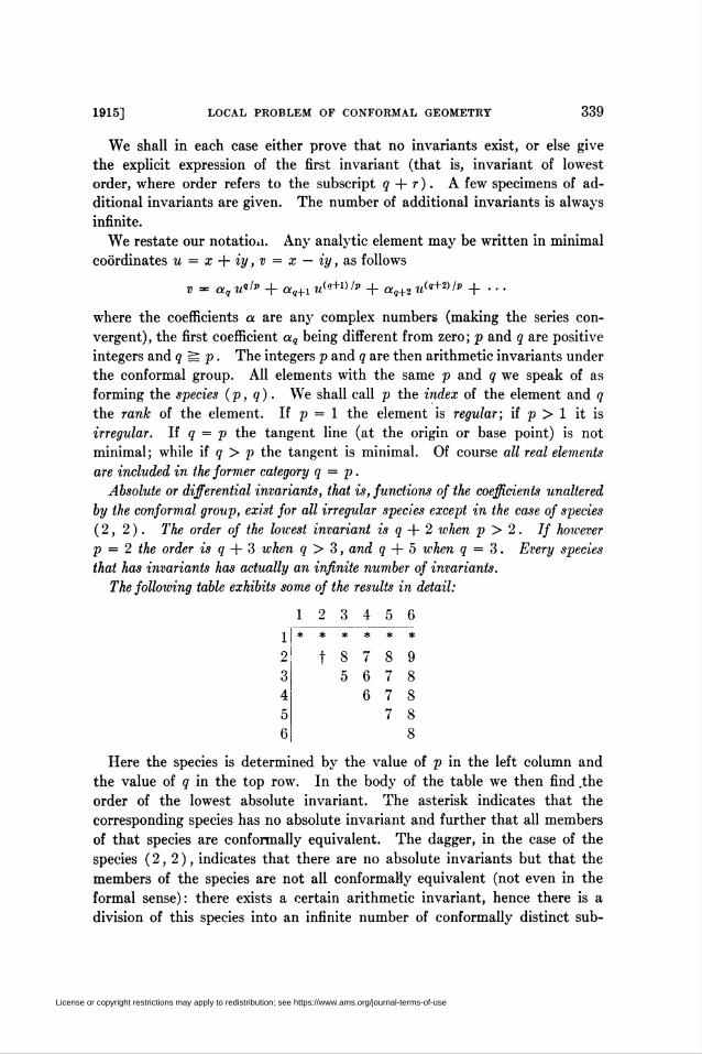
of species (p, q), namely

(1) v = aq ««'* + aq+i «<«+»/»• + aq+2 w<«+2>/p + • • • (a, * 0),

we inquire when this element is equivalent to some other element of the

same species

(2) V = AqU*l" +Aq+i W+»'' + Aq+2W«+»I'> + .... (¿1 + o).

Equivalence means that the first equation can be converted into the second

by a transformation of the form

U = a[u + a'2u2 + • • •,

(3)V = b[v + b'2v2 + ■ • •,

in which neither a\ nor b[ is to vanish since the transformation is to be regular

at the origin. We shall find it convenient to write our transformation in the

less symmetric form

u = ai U + a2 U2 + ••• (a, +0),

(4)V = biv + b2o2+ ••• (&i+0),

where the a's are of course the coefficients of the series obtained by reverting

the first series in (3).

To express the fact that (4) converts (1) into (2) we may eliminate the three

quantities u, v, V from the four equations (1), (2), (4). The result is an



equation in U which must hold identically, so that we may equate coefficients

of like powers. In order to avoid fractional exponents we make the substi-

tution

(5) U = fp;

our fundamental condition of equivalence then takes the form

(6) Aq t* 4- Aq+i t"+1 4- ■■■ = 6! P 4- 62 P2 4- • ■ ■,

where

P = aq t" («1 4- «2 V 4- «3 f2p 4- • ■ • )qlp

(6')+ aq+i f«+1 («! + «2 P 4- «s f2* + • • • )(9+1)/p + • • • ,

which can obviously be developed as a series in integral powers of t, beginning

with tq, since ai does not vanish.

Equating coefficients of like powers of f in (6), we obtain an infinite set of

equations involving the constants a and A of the two curves and the constants

a and 6 of the transformation. Two given curves (1) and (2) will be equivalent

provided this infinite set of equations can be solved for the «'s and 6's, subject

of course to the essential restriction «1 4= 0, 61 4= 0.

If for all values of the a's and A's, the a's and 6's can be found, then the

curves are always equivalent and no invariants exist. Otherwise certain

conditions must be imposed on the a's and ^4's in order to render the equations

consistent, and this indicates the existence of invariants. Which of these

possibilities actually occurs we shall find depends essentially on the values of

integers p and q determining the species. Some species have invariants,

others have not.

The integers p and q are obviously of invariant character under the con-

formal group. In some types other such arithmetic invariants exist. But our

main question is to find absolute or differential invariants, that is, expressions

depending on a finite number of the coefficients of the curve, say aq up to

aq+r, which are unchanged by conformai transformations, and thus are

converted into expressions of the same form in the new coefficients Aq up

to Aq+r. The principal result obtained (proofs are given later) is as follows:

The regular species (1, 1), (1,2), (1,3), •--, have no differential invari-

ants. But with the single exception of the species (2,2), all the irregular species

have differential invariants.

When p = 1, there are no invariants; also when p = 2 and « = 2 there

are no invariants; but in all other cases the analytic element (1) has invariants.

We shall divide our discussion into three parts, namely, p = 1, p = 2,

p > 2. The first and third cases are very simple; but the second is some-

what complicated, since we shall find that distinct discussions are required

for three subcases, namely, « = 2,« = 3,«>3.



We shall in each case either prove that no invariants exist, or else give

the explicit expression of the first invariant (that is, invariant of lowest

order, where order refers to the subscript a + r). A few specimens of ad-

ditional invariants are given. The number of additional invariants is always

infinite.

We restate our notation. Any analytic element may be written in minimal

coordinates u = x + iy, v = x — iy, as follows

v = aq M«'" + aq+i u^+^'p + aq+2 îî<«+2)/p + ■■■

where the coefficients a are any complex numbers (making the series con-

vergent), the first coefficient aq being different from zero; p and a are positive

integers and a 15 p. The integers p and a are then arithmetic invariants under

the conformai group. All elements with the same p and a we speak of as

forming the species (p, q). We shall call p the index of the element and q

the rank of the element. If p = 1 the element is regular; if p > 1 it is

irregular. If a = p the tangent line (at the origin or base point) is not

minimal; while if a > p the tangent is minimal. Of course all real elements

are included in the former category q = p.

Absolute or differential invariants, that is, functions of the coefficients unaltered

by the conformai group, exist for all irregular species except in the case of species

(2, 2). The order of the lowest invariant is q + 2 when p > 2. If however

p = 2 the order is q + 3 when q > 3, and q + b when q = 3. Every species

that has invariants has actually an infinite number of invariants.

The following table exhibits some of the results in detail:

12 3 4 5 6

t 8 7 8 95 6 7 8

6 7 8

7 8

Here the species is determined by the value of p in the left column and

the value of q in the top row. In the body of the table we then find .the

order of the lowest absolute invariant. The asterisk indicates that the

corresponding species has no absolute invariant and further that all members

of that species are conformally equivalent. The dagger, in the case of the

species (2,2), indicates that there are no absolute invariants but that the

members of the species are not all conformally equivalent (not even in the

formal sense): there exists a certain arithmetic invariant, hence there is a

division of this species into an infinite number of conformally distinct sub-


340 EDWARD kasner: [July

species. See § 6 below. We recall that all real curves are included in the

species (1,1), (2, 2), (3,3), etc.; all real regular curves are included in

(1,1).When p > 2, the lowest invariant is a function of the first three coefficients

aq, aq+i, aq+2. When p = 2 and q > 3, the lowest invariant involves the

first four coefficients. Finally when p = 2 and q = 3, the result involves six

coefficients.

§ 3. Discussion for p > 2

This is extremely simple, for we find that the first three equations obtained

by the process already described, equating coefficients in the fundamental

equation (6), involve only two of the transformation constants. The equa-

tions are in fact

Aq = aq 6i a«'2, Ai+i = aq+i bi a<«+»/2, Aq+2 = aq+2 6i a<*+2>/2.

Eliminating ai and 6i, we find

<Xq aq+2 _ Aq_Aq+22 — At •

«?+i Aq+l

Hence when the index p of the analytic element (1) is greater than two the invariant

of lowest order is

aq aq-r2

«;+, ;

the order = q 4- 2, weight = 2q 4- 2, degree = 2.

§ 4. Discussion for p = 2, q > 3

In this case the first two equations

Aq = aq bi a"'2, Aq+i = «9+1 6i «<«+1>/2

determine as before the values of «i and 6i. The next two equations

Aq+2 = «8t2 bi a<i<+2"2 4- \ aq 6i «<«+2> I2 «2,

Aq+3 = aq+3 bi a<«+3>/2 + \ aq+i 6X a<«-»/2 «2

bring in only «2, not 62. Eliminating ai, 6i, and a2 from our four equations

and separating the coefficients a and A, we find

When p equals two and q is greater than three, the irregular element of species

(p, q) has the following invariant of lowest order

aq (aq «g+3 — aq+i aq+2)

«î+i

Order = q 4- 3, weight = 3g 4- 3, degree = 3.



§ 5. Discussion for p = 2, a = 3

We shall now show that an ordinary cusp with a minimal tangent line has

a differential invariant. This is the species defined by p = 2, q = 3 ; that is

V = «3 U3 + «4 W + a5 W +

We shall need the first six equations obtained in the usual way from the

equivalence identity. They are

6i a3 = Az af, 6i ai = A4 af2, bi ab = \Az ai'2 a2 + Ab af,

6i ao + b2 a\ = 2 Ai ai a2 + A6 a\ß,

bi «7 + 2b2 a3 ai = A3 ( far"2 o¡ + fa1/2 a3 ) + f A, af a2 + A7 af,

6i aB + b2(al + 2a3 a5) = ^44 (a2 + 2ai a3) + 3A6 a? a2 + Aa a*.

We are now trying to prove the existence, not the non-existence of invariants ;

hence it is necessary to have these equations in full, not merely in leading

terms, as will be the case in § 6.

The first two equations involve two transformation coefficients ai, bù the

next two bring in two new coefficients a2, b2; but the following two bring in

merely a3, since b3 does not as yet appear. Hence it is possible to eliminate the

transformation coefficients, and obtain a relation between the coefficients

a3 • • • as of the old curve, and the coefficients A3 • • • As oí the new curve.

Carrying out the elimination we find that the two sets of coefficients may be

separated,* the result being the expression

a\ ( 0a3 a4 a7 — 3al ap — 22a4 a\ — Pal a8 + 180:3 «5 ao ) + 4a3 a\ «5

«Ïequal to the same expression in the ^4's.

Hence this expression is an absolute invariant of our element of species

(p = 2,a = 3). It is of order 8, weight 20, and degree 5.

In cartesian coordinates such an irregularity is represented by

y = ix + c3 a:3 + c4 x* +

It is not usually possible to reduce this conformally to the simple cubic cusp

y = ix + xi

with minimal tangent line. A necessary condition is that the absolute in-

variant (a certain combination of C3, c¡,, Co, c-¡, c$) shall have a special

numerical value, t

* This calculation was carried out by Mr. J. A. Northcott in my seminar at Columbia

University, 1913.

t The special case where at vanishes of course defines an invariant subspecies under the

given species, the first absolute invariant then becoming infinite. An invariant of higher

order may then be found for this special case (see § 8).


342 Edward kasner: [July

§ 6. Discussion for p = 2, q = 2

We now prove that the species p = 2, « = 2, namely

v = a« id 4- a3 m3 4" «i w* 4- • • • ,

has no differential invariants, making first the assumption a3 4= 0.

The equivalence identity takes the form

6i P 4- 62 P2 + ■ • • = A212 4- A3 f3 + • • •,

whereP =• P2 f2 + P3 f3 + • • • ,

the coefficients here being

P2 = a2 «i, P3 = a3 a]12, Pi = a2 a2 4- • • • ,

P5 = |o¡3 «î'2 «2 4- • • • , Po = a2a3 4- • ■ ■ , Pi = f «3 «'/2 «3 4- • • • ,

Only the leading terms, that is terms involving the « of highest subscript,

are written out since the other terms are unnecessary for the present purpose.

Equating coefficients of powers of f in the identity, we have an infinite

system of equations involving the constants a and A of the two arbitrary

curves, and the constants a and 6 of the transformation. We must show

that these equations can always be solved for the a's and 6's, with neither

ai nor 6i vanishing.

The first pair of equations, arising from f2 and f3, is

a2 ai 6i = A2,

a3 «f h = A3,giving the unique solution

(A3a2\2 A32a¡

\ A2 a3 ) A3 a2

finite and different from zero, since the first two terms in the series for the

curves are assumed to be actually present.

The next pair of equations, arising from f4 and f5, are linear in two new

unknowns, «2 and 62, the determinant of the left hand members being

a2 6i a2 ai

|a3 a1/2 6i 2a2 «3 as

To show that this does not vanish, we may cancel out the non-vanishing

factors, a2, a3, «i, 6i; the remaining purely numerical factor is found to be

3 9 - 2 ■2 - I



Similarly the next pair of equations bring in linearly two new unknowns,

a3 and 63, and the numerical factor in their determinant is

1 132

It is easily verified that the nth pair of equations, arising from the terms

t2n and t2n+1, always bring in just two new unknowns, a„ and bn, and that these

equations admit a unique solution, since the determinant, factorable into

powers of a2, a3, ai,bi, together with the number

1 13 *, = n - f,

cannot vanish.

It follows that the coefficients of the transformation cannot be eliminated

from the first 2n equations, no matter how great we take n. Hence there

cannot be any invariant relations involving a finite number of coefficients of

the two curves. It follows that our curve can be reduced formally to the

normal form v = w?, and that this reduction is unique.

So far we have used the assumption 0:3 4= 0, that is, that the term u* is

actually present. Since we are discussing the class p = 2, q = 2 the term u$

must of course be present; that is a2 + 0. Let us now consider what happens

if any number of successive terms after the first are absent.

Let k = 2m + 1 denote the subscript of the first term with a fractional

exponent actually appearing in the series for the curve. The equation of

the curve is thus of the form

v = a2u + a4u2 + ■ ■ • + aim um + a2m+i um+i- + • • • .

The polynomial of mth degree in the first part of this development can always

be transformed into a linear term. Hence we may, without loss of generality,

take our curve in the reduced form

v = a2 w* + ak ukl2 + ak+i u{k+l) l2 + ■ ■ ■ ,

where k = 2m + 1 is odd, and a2 + 0, ak 4= 0.

We must show that such a curve can always be transformed into an arbitrary

curve of the same type

V = A2W + Ak Uk>2 + Ak+i <7<*+1> l2+ ■■■.

The equivalence identity is

61 P + 62 P2 + • • • = A2t2 + Aktk+ ■■■,

where

P = a2axt2 + («2a2 + v)¿4+ (a2a3+ •••)r5+ ••• +aka\l2tk

+ {\ak a<*-2>/2 a2 + • • • ) tk+2 + (|a* a?-2»2 a3 + • • • ) • tk+l +■■■.

Trans. Am. Math. Soc. 23



Here again only the leading terms with respect to the coefficients a are needed.

Writing out the system of equations obtained by equating coefficients of

like powers of f, we find that the first two unknowns ai, 61, are not, as in the

former case, given by the terms in f2 and f4, but rather by those in f2 and tk.

These equations are not linear but give non-vanishing values for «i and 61.

The next pair of equations, linear in a2 and 62, are given by the terms f4

and tk+2. In general the unknowns an and 6„ are determined by a pair of

linear equations, arising from the terms in f2n and z^4"2*"-1). The determinant

involves as a factor, in addition to powers of ai, 61, a2, ak which do not

vanish, onlv the number1 1

k= n—2

which can never vanish since k is odd.

Therefore the type considered has no absolute invariants. The only dis-

tinctions are those that arise from the variation of the integer k — 2m 4- 1 •

Any curve can be converted into any other having the same value of m.

Every irregular element of species p = 2, q = 2 can be reduced* to the normal

formV = M 4- wm+i

where mis a positive integer 1,2,3, • • • . There are no differential invariants.

The only arithmetic invariant is the integer m.

The transformation converting the curve into the normal form is deter-

minate, but not always uniquely determinate. This is due to the fact that

the first pair of equations, that is those giving «i and 61, are non-linear, at

least with respect to ai. The equations are

a2 ai 61 = A2, ak a?+1 61 = Ak,

and have 2m — 1 solutions

(Akc*}^ , _A1ai-\A2ak) ' bl~ ai-as

Only when m = 1 is the required reducing transformation unique.

In particular the number of transformations converting one of our curves

into itself is 2m — 1. The only transformation of v = u 4- u* into itself

is identity, f

* The question of convergency is left open for future discussion. This does not, of course,

affect results as to the existence or non-existence of invariants (that is, differential invariants

of finite order). See paper on Conformai geometry cited in § 1.

t We refer throughout only to direct conformai transformations. It may be shown that there

is also a unique reverse conformai transformation which converts this curve into itself. The

general reverse (or improper) conformai transformation is represented in minimal coordinates

by writing U as a series in v, and F as a series in u.



If we pass from the notation of minimal coordinates u, v to that of cartesian

coordinates x, y we may express our results as follows:

The class of curves (analytic elements) defined by p = 2, q = 2, that is curves*

having a cartesian equation of the form

y = c3 x% + Ci x* + c5 z} + • • • ,

Aas no differential invariants under the conformai group. Such a curve can be

reduced^ conformally to the normal form

y = xm+* (to = 1,2,3, •••)•

The only conformai distinctions are with respect to the arithmetic invariant m.

The number of direct conformai transformations of this normal form into itself

is 2m — 1.

Geometrically, the type of irregularity defined by p = 2, q = 2 is that of

an ordinary cusp, with a non-minimal tangent. Variation of m signifies a

difference in the (fractional) order of contact between the curve and its tangent

line. The case m = 1, leads to the simplest cusp, represented by the semi-

cubic parabolay = xK

If we apply a conformai transformation to this, we obtain an analytic curve

with a cusp of the same kind

y = c3 x* + d x* + • • • (es + 0).

Since m = 1, the transformation is uniquely determined by the curve. Hence

have this peculiar result:

// we know the effect of a conformai transformation (of course assumed regular

in the neighborhood of the cusp) on the points of the semi-cubic parabola (or any

conformally equivalent curve), that is if we know the equation of the new or trans-

formed curve, the transformation is uniquely determined, t

This is apparently the simplest possible way of specifying (completely deter-

mining) a conformai transformation by means of curves.

7. Discussion for p = 1. Regular Elements

In this simple case there are no differential invariants. This is well-known

for the species ( 1, 1 ), that is, when the initial tangent is non-minimal. It

is true also when the tangent is minimal, that is when a is greater than unity,

as we shall show below.

* We take the tangent as axis of x and the normal as axis of y. This is legitimate since

the tangent is non-minimal.

t At least in the formal sense.

t Contrast this with the familiar theorem : If we know the effect of a conformai trans-

formation on the axis of reals, y — 0, the transformation is not determined but involves an

infinitude of arbitrary constants.



Regular elements have no differential invariants under the conformai group.

All the elements of the same species (p — 1, q = k), that is,

v = akuk 4- ak+i uk+l 4- ■■■ ,

are equivalent to each other, being reducible to the normal form

V = Uk;

so that arithmetic invariant k is the only invariant.

To prove this we may of course use the general identity (6). But we find

it more convenient here to use the following simpler method, which settles

at the same time all convergency questions.

To show that the given curve can be reduced to the normal form stated,

it is sufficient to assume that v is unaltered, and to seek the proper trans-

formation of u. Fsing

U = g i u ), V = v,

we find that the function g must satisfy the relation

g(u) = u \ak 4- ak+i u 4- ak+2 u2 4-

Since ak 4= 0, this formula defines an integral power series and the coefficient

of u in the result does not vanish. Hence our conformai transformation

exists.

The number of possible transformations is infinite, depending on an infinite

set of arbitrary coefficients. To show this, it is sufficient to seek the most

general transformation

U = «i u 4- a2u2 4- ■ ■ ■ ,

T ' = 6i v 4- b2 v2 4- ■ ■ ■,

which converts the canonical curve V = Uk into itself. The requisite con-

dition is

«i 4- a2 u 4- a3u2 4- ■ ■ ■ = a/6i 4- 62 uk 4- b3 u2k 4- ■ ■ ■ ,

which can be satisfied by taking the 6's arbitrarily with 6i 4= 0; then finding

the a's, which are (up to a /r-th root of unity) determined.*

7f is thus seen that any curre of species (1, k) can be converted conformally

into any curve of the same species in an infinity ( °o °° ) of ways. If we take not

only the two curves at random but also an arbitrary regular analytic correspmdence

between their points (the origin going into the origin) the conformai transformation

exists and is uniquely determined.

Of course in the real conformai plane the only regular elements are those

* On the other hand it is not possible, when k exceeds unity, to take the a's arbitrarily and

then find the b's.



of species ( 1, 1 ), that is to say k is then unity. The results are then well-

known.

The natural conformai classification of regular analytic elements in the

complex plane, expressed in the usual cartesian apparatus, is as follows:

Every regular analytic element in the complex plane can be reduced to one of

these three forms:

(i) y = o,

(II) y = ix + Xk (k = 2, 3, 4, •••),

(III) y = ix.

The first is of course the most general form: it contains all elements whose

tangent line is non-minimal (including as a special case all real elements.)

The second includes all curved elements whose tangent line is minimal, the

order of contact with the minimal line being k — 1. The third is the most

special form; it includes merely the minimal straight lines of the plane.

In a previous paper,* the author showed that regular elements may be

completely characterized, with respect to conformai equivalence, by the value

of the limit of the ratio of the arc to the chord running from the given base

point to a neighboring point. For ordinary curves, that is, class (I), this limit

is of course unity. But for class (II) the result is

arc 2 Vfechord k + 1 '

which is, for example, correct to two decimal places, .94 for k = 2, .86 for

k = 3, .80 for k = 4, .74 for k = 5. Hence the value of L determines the

value of the integer k, so that two elements having the same L will be con-

formally equivalent. Finally, for class (III) both arc and chord vanish iden-

tically, hence the limit L does not exist (is indeterminate).

§ 8. Some Additional Invariants

For each species (p, q) we have either shown that no invariants exist or we

have obtained the explicit expression of the first absolute invariant (differential

invariant of lowest order). Every species that has an invariant (that is every

irregular species except (2, 2)) has in fact an infinite number of invariants.

We shall here give some examples of the invariants of higher order.

Consider first the species ( 3, 3 ), that is

(7) v = a3 w' + a4 u* + a¡, u* + • • • ( «3 =t= 0 ).

Here the first invariant, obtained by elimination from three equations, is,

in accordance with the discussion for p > 2 given in § 3,

* The ratio of the arc to the chord of an analytic curve need not approach unity. Bulletin

of the American Mathematical Society, vol. 20 (1914), pp. 524-531.



a3 a3

«4

Assuming that a4 does not vanish, we find that we can also eliminate the

constants of the transformation from the next three equations, the result

being an invariant of order 8. Continuing in this way by grouping the

equivalence equations into sets of three we find this result:

The general case of species ( 3, 3 ), that is form (7) with a4 4= 0, has absolute

invariants of order 5, 8, 11, 14, efc.

In the more special case defined by a4 = 0, a5 4= 0, we find that there

still exist an infinite number of invariants, the orders now being 7, 10, 13,

16, etc.

For larger values of p, the structure of a certain first succession of p — 2

invariants is very simple. Thus for p = 5, the first three invariants are

aq aq+2 aq aq+3 aq aq+i

a*+i ' aq+iaq+2' aq+i aq+3 '

The next higher invariants are more complicated.

For the species (3,4), we have first a simple invariant of order 6, and

second a complicated invariant of order 9. The expressions are

a4 a6 a\ ( 5a2. a7 — 4a4 a5 a8 4" 2a{ a9 — 3a4 a6 a7 )

«5 ' «5

For the species (4,5) the first three invariants, of orders 7,8, and 11, are

ah a7 «6 «8 12a3 a\ a9 — 7a* a7 a9 — 10a4 a6 aio 4- 5a' an

In our discussion of lowest invariants the most complicated species was

( 2, 3 ), since here it was necessary to use six equations before elimination

was possible. Grouping the next equations of equivalence into sets of six,

we find that new eliminations are always possible. Hence

The species (2,3) has an infinite number of invariants, the orders being

8, 14, 20, 26, efc.

This is of course in the general case of that species. It is assumed that

not only the first term a3 m§ is present, but also the second term a4 m* . Separ-

ate discussions are necessary if certain terms are absent.

For the arbitrary species (p, q) with a certain number of terms, after the

first, absent, we state only this result. If the curve is of the form

v = aq u«'* 4- aq+k u<-*+k)I' 4- aq+k+i «<«+*+« '"4-,

where p > 2 and k < p — 1, the first invariant is

aq aq+k+i



For the real species (p, p) it is worth while to give the following more

detailed results.

The case represented by

v = aq u*'* + aq+k u^k) '* + ■ ■ ■ ,

when k < p — 1 has a first invariant of order p + k + 1 and also, provided

k < p — 2, a second invariant of order 2p — 1. When k = p — 1, the

first invariant is of order 2p + 1.

If still more terms in the power series are absent, say if av+i = 0, av+2 = 0,

and so on, until aip+k + 0, so that the element ( p, p ) is of the special form

V = aa W"" + aiq+k m(íp+*> lk +

then when k < p — 1 the first order is Ip + k + 1; and when k = p — 1,

assuming p > 2, the first order is (¿ + l)p + 1.

§ 9. Real Elements

For real elements under the group of real conformai transformations we

may, in conclusion, state our principal results in the usual cartesian coordinates

as follows, taking the base point as origin and the initial tangent of the ele-

ment as axis of x.

Regular real elements are conformally reducible to y = 0.

Irregular real elements of index two, that is

y = c3 xi + d xi + •■•

have no differential invariants, and may be reduced (formally) to

y = xm+i, (m = 1,2,3, ■■■).

Irregular real elements of index greater than two always have an infinite num-

ber of differential invariants under the real conformai group.

A direct discussion of the real theory in cartesian coordinates will appear

in another paper. It should be observed that our classification into species

(p, q) is based on the minimal notation u, v. If we pass to the cartesian

notation x, y, the fractional exponents in the leading term are usually different

from q/p. The index p remains as denominator, but the new numerator has

no intrinsic significance. A new arithmetic invariant is then obtained which

has such significance.

Columbia University, New York.


Date post:	15-Mar-2020
Category:	Documents
Upload:	others
View:	13 times
Download:	0 times

CONFORMAL CLASSIFICATION OF ANALYTIC ARCS OR …...CONFORMAL CLASSIFICATION OF ANALYTIC ARCS OR...

Documents