The Blasius Function:Computations BeforeComputers, the Value of Tricks,Undergraduate Projects, andOpen Research Problems∗
John P. Boyd†
Abstract. The Blasius flow is the idealized flow of a viscous fluid past an infinitesimally thick, semi-infinite flat plate. The Blasius function is the solution to 2fxxx + ffxx = 0 on x ∈ [0,∞]subject to f(0) = fx(0) = 0, fx(∞) = 1. We use this famous problem to illustrate severalthemes. First, although the flow solves a nonlinear partial differential equation (PDE),Toepfer successfully computed highly accurate numerical solutions in 1912. His secretwas to combine a Runge–Kutta method for integrating an ordinary differential equation(ODE) initial value problem with some symmetry principles and similarity reductions,which collapse the PDE system to the ODE shown above. This shows that PDE numericalstudies were possible even in the precomputer age. The truth, both a hundred years agoand now, is that mathematical theorems and insights are an arithmurgist’s best friend, andthey can vastly reduce the computational burden. Second, we show that special tricks,applicable only to a given problem, can be as useful as the broad, general methods thatare the fabric of most applied mathematics courses: the importance of “particularity.” Inspite of these triumphs, many properties of the Blasius function f(x) are unknown. Wegive a list of interesting projects for undergraduates and another list of challenging issuesfor the research mathematician.
Thinking is the cheapest and one of the most effective long-range weapons.–Field Marshal Sir William Slim, 1st Viscount Slim (1891–1970)
1. Introduction. Slim’s maxim applies as well to science as to war. The Blasiusproblem of hydrodynamics is a good illustration of how cunning can triumph overbrute force.
The Blasius flow of a steady fluid current past a thin plate is the solution of thepartial differential equation (PDE)
(1.1) ψY Y Y + ψX ψY Y − ψY ψXY = 0, X ∈ [−∞,∞], Y ∈ [0,∞],
where subscripts with respect to a coordinate denote differentiation with respect to the
∗Received by the editors February 1, 2007; accepted for publication (in revised form) February 7,2008; published electronically November 5, 2008. This work was supported by NSF grants OCE0451951 and ATM 0723440.
http://www.siam.org/journals/sirev/50-4/68159.html†Department of Atmospheric, Oceanic and Space Science, University of Michigan, 2455 Hayward
Avenue, Ann Arbor, MI 48109 ([email protected], http://www.engin.umich.edu/∼jpboyd/).791
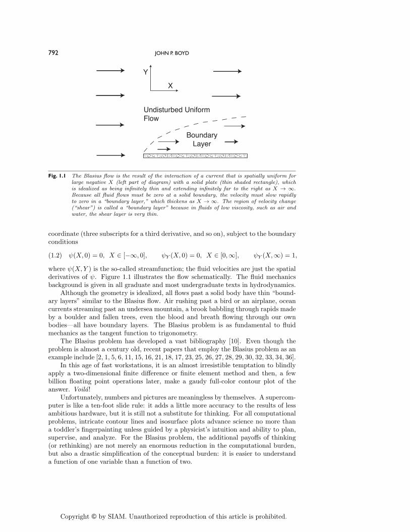
Fig. 1.1 The Blasius flow is the result of the interaction of a current that is spatially uniform forlarge negative X (left part of diagram) with a solid plate (thin shaded rectangle), whichis idealized as being infinitely thin and extending infinitely far to the right as X → ∞.Because all fluid flows must be zero at a solid boundary, the velocity must slow rapidlyto zero in a “boundary layer,” which thickens as X → ∞. The region of velocity change(“shear”) is called a “boundary layer” because in fluids of low viscosity, such as air andwater, the shear layer is very thin.
coordinate (three subscripts for a third derivative, and so on), subject to the boundaryconditions
where ψ(X,Y ) is the so-called streamfunction; the fluid velocities are just the spatialderivatives of ψ. Figure 1.1 illustrates the flow schematically. The fluid mechanicsbackground is given in all graduate and most undergraduate texts in hydrodynamics.
Although the geometry is idealized, all flows past a solid body have thin “bound-ary layers” similar to the Blasius flow. Air rushing past a bird or an airplane, oceancurrents streaming past an undersea mountain, a brook babbling through rapids madeby a boulder and fallen trees, even the blood and breath flowing through our ownbodies—all have boundary layers. The Blasius problem is as fundamental to fluidmechanics as the tangent function to trigonometry.
The Blasius problem has developed a vast bibliography [10]. Even though theproblem is almost a century old, recent papers that employ the Blasius problem as anexample include [2, 1, 5, 6, 11, 15, 16, 21, 18, 17, 23, 25, 26, 27, 28, 29, 30, 32, 33, 34, 36].
In this age of fast workstations, it is an almost irresistible temptation to blindlyapply a two-dimensional finite difference or finite element method and then, a fewbillion floating point operations later, make a gaudy full-color contour plot of theanswer. Voila!
Unfortunately, numbers and pictures are meaningless by themselves. A supercom-puter is like a ten-foot slide rule: it adds a little more accuracy to the results of lessambitious hardware, but it is still not a substitute for thinking. For all computationalproblems, intricate contour lines and isosurface plots advance science no more thana toddler’s fingerpainting unless guided by a physicist’s intuition and ability to plan,supervise, and analyze. For the Blasius problem, the additional payoffs of thinking(or rethinking) are not merely an enormous reduction in the computational burden,but also a drastic simplification of the conceptual burden: it is easier to understanda function of one variable than a function of two.
2.1. PDE to ODE. Blasius himself noted in his 1908 paper that if ψ(X,Y ) is asolution, then so is
(2.1) Ψ(X,Y ) ≡ c ψ(c2X, cY ),
where c is an arbitrary constant. In other words, this implies that the problem hasa continuous group invariance. The streamfunction is not a function of X and Yseparately, but rather must be a univariate function of the “similarity” variable
(2.2) x ≡ Y√X.
Any other dependence on the coordinates would disrupt the group invariance. Thereis some flexibility in the sense that one could replace x by x2 or any other smoothfunction of x as the similarity variable, but the most convenient choice, and thehistorical choice, is
(2.3) ψ(X,Y ) =√X f(Y/
√X)
for some univariate function f .Thus, Blasius showed that the PDE (1.1) could be converted to the ODE
(2.4) 2fxxx + ffxx = 0
subject to the boundary conditions
(2.5) f(0) = fx(0) = 0, fx(∞) = 1.
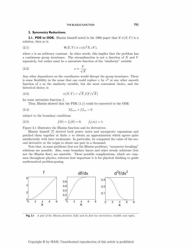
Figure 2.1 illustrates the Blasius function and its derivatives.Blasius himself [7] derived both power series and asymptotic expansions and
patched them together at finite x to obtain an approximation which agrees quitesatisfactorily with later treatments. In particular, he computed the value of the sec-ond derivative at the origin to about one part in a thousand.
Note that, in some problems (but not the Blasius problem), “symmetry-breaking”solutions are possible. Also, some boundary layers and other steady solutions (butnot the Blasius flow) are unstable. These possible complications, which are com-mon throughout physics, reiterate how important it is for physical thinking to guidemathematical problem-posing.
0 2 4 6 80
2
4
6
0 2 4 6 80
0.2
0.4
0.6
0.8
0 2 4 6 8
0.1
0.2
0.3
f df/dx d2f/dx2
x x x
Fig. 2.1 A plot of the Blasius function (left) and its first two derivatives (middle and right).
2.2. Conversion of the Boundary Value Problem to an Initial Value Prob-lem. Boundary value problems must be solved at all points simultaneously (a “jury”problem), whereas an initial value problem can be solved by a stepwise procedure (a“marching” problem). In this sense, initial value problems are easier. The BlasiusODE could be converted into an initial value problem and integrated by marchingfrom x = 0 to large x if only
(2.6) κ = fxx(0)
were known. Karl Toepfer [35] realized that knowledge of κ is in fact unnecessary.The reason is that there is a second group invariance such that if g(x) denotes thesolution to the Blasius equation with g(0) = 0, gx(0) = 0, and its second derivative isarbitrarily set equal to one, then the solution with fxx(0) = K is
(2.7) f(x;K) = K1/3 g(K1/3x).
It therefore suffices to compute g(x) and then rescale both the horizontal and verticalaxes of the graph of g(x) so that the rescaled function has the desired asymptoticbehavior at large x, namely, fx(∞) = 1. The true value of the second derivative atthe origin is then
(2.8) κ = limx→∞
gx(x)−3/2.
With Toepfer’s trick, it is only necessary to solve the differential equation as aninitial value problem once. At two large but finite xj , ordered so that xj > xj−1,compute κj ≡ (1/gx(xj))3/2. If the κj closely agree, κ is approximately equal to thecommon value of the κj ; if they are far apart, march to still larger x and try again.Using a Runge–Kutta method with a grid step of 1/10 and the endpoints of x1 = 4and x2 = 6, Toepfer was thus able to determine κ correctly to about one part in110,000!
Freshman physics books are populated with analytical solutions, but none has everbeen found for the Blasius equation. The first general-purpose electronic computer,ENIAC, was more than a third of a century in the future when Toepfer did hiswork. Nevertheless, by exploiting group invariances, he reduced the Blasius problemto perhaps a couple of hundred multiplications and additions. Though he does notrecord his paper-and-pencil computing time, it was likely only an afternoon.
3. Lessons from Symmetry Reductions and the Numerical Solution.
3.1. When Computers Were Human.In conducting extensive arithmetical operations, it would be natural toavail oneself of the skill of professional [human] computers. But unfortu-nately the trained computer, who is also a mathematician, is rare. I havethus found myself compelled to forego the advantage of the rapidity andaccuracy of the computer, for the higher qualities of mathematical knowl-edge and judgment.
–Sir George C. Darwin (1845–1912) [14, p. 101]
The Blasius–Toepfer numerical work was only a tiny part of the vast computationsperformed before the advent of electronic computers. Much of the number-crunchingwas done by full-time human calculators known as “computers.” Grier [20], Croarken[12], and others [3, 13] have written very readable accounts of the heroic age of number-crunching. A substantial portion of the “computers” were female—none of this “girlscan’t do math” nonsense in the eighteenth or nineteenth century.
Weyl [39, p. 385] wrote that the Blasius problem “was the first boundary-layerproblem to be numerically integrated . . . [in] 1907.” However, the history of numericalsolutions to differential equations is much older and richer. More than two decadesbefore Blasius, John Couch Adams devised what are now called the Adams–Bashforthand Adams–Moulton methods for numerically integrating an initial value problem [4].Toepfer numerically integrated the Blasius problem using a Runge–Kutta methodpublished by Runge in 1895 and greatly refined by Kutta in 1901.
Aspray notes in his preface to Computing Before Computers [3], “Wherever weturn we hear about the ‘Computer Revolution’ and our ‘Information Age’. . . . Withall of this attention to the computer we tend to forget that computing has a richhistory that extends back beyond 1945.” Similarly, Gear and Skeel [19] note thatthe post–World War II development of electronic computers “has, of course, affectedthe algorithms used, but this has resulted in surprisingly few innovations in numericaltechniques.” What they mean is that although numerical algorithms have been greatlyimproved and advanced since the first electronic computers were built in the late 1940s,the building blocks—Runge–Kutta, Lagrangian interpolation, finite differences, etc.—were all created in the precomputer age. For example, Lanczos published his greatpaper, which is the origin of both Chebyshev pseudospectral methods and the taumethod, in 1938 [24]. Rosenhead’s point vortex paper was published even earlier [31].George Boole’s book [8] on finite differences first appeared in 1860!
Howarth’s 1938 article, which contains an extensive table of the Blasius f(x) andits first two derivatives, contains the acknowledgment, “I wish to express my gratitudeto the Air Ministry for providing me with a [human] computer to perform much of themechanical labour” [22]. But his calculations by government-funded human computerhad long antecedents. Sir George Darwin, legendary for his prodigious numerical cal-culations in celestial mechanics and the equilibria of self-gravitating stars and planets,independently reinvented some of Adams’ methods and used them to compute peri-odic orbits in 1897 [14]. He noted sadly that his previous human computer had died,but he found two new helpers at Cambridge and did much of the calculating him-self. Foreshadowing Howarth, he thanked a grant from the Royal Society for fundingtwo-thirds of the cost of this monumental number-crunching.
This brief history, though omitting many other examples, shows that computinghas never been primarily about electronics, but always primarily about mathematics,algorithms, and organization, plus money for the he/she/it which is the “computer.”
3.2. Precomputing.
Computing is a temptation that should be resisted as long as possible.–John P. Boyd in the first edition of his book
Chebyshev and Fourier Spectral Methods(Springer-Verlag, 1989)
Presoaking is a sound strategy for washing pots and pans with burnt or driedresidues. In a similar way, successful computing is dependent on precomputing: iden-tifying symmetries and other mathematical principles that can greatly reduce thescope of the problem. Engineers have relied for generations on dimensional analysisand the Buckingham pi theorem, which assert that physics must be independent of thesystem of units. Thus, a problem with three dimensional parameters can be reducedto the computation of a function that depends on only one parameter or perhaps noparameters at all.
Good algorithms are vital, but intelligent formulation of the numerical problem isequally important. Unfortunately, the vast expansion of numerical algorithms, soft-
ware management, and parallel computing has rather crowded out of the curriculumthe tools of twentieth century applied mathematics: singular perturbation theory,group theory, special functions, and transformations. The Blasius problem is butone of many examples where these fading tools reduced the computational burden byan order of magnitude and greatly simplified the description of results. A centuryof progress in floating point hardware has not reduced the need for problem-specificthinking, but rather merely increased our number-crunching ambitions.
4. Known Properties.It is important to make friends with the function.
–Tai Tsun Wu, Gordon McKay Professor of Applied Physics, Harvard
Before we can dive into the virtues of “particularity,” we need to “make friends”with the Blasius function. As archaeologists reconstruct a lost civilization one potteryshard at a time, so applied mathematics accumulates understanding through a slowaccretion of individual properties.
4.1. Power Series. The power series begins
(4.1) f(x) ≈ κ
2x2 − κ2
240x5 +
11161280
κ3x8 − 54257792
κ4x11 + · · · ,
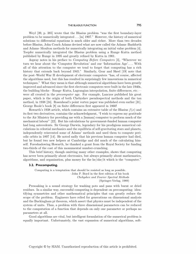
where κ is the second derivative of the function at the origin, given to very highprecision in Table 4.1. Only every third coefficient is different from zero. As provedin introductory college calculus, a power series converges only within the largest disk,centered on x = 0, which is free of singularities of f(x). Although it would take ustoo far afield to recapitulate the proof here, the Blasius function has a singularity onthe negative real axis [10] at x = −S, where no closed form for S is known. The seriesconverges for |x| < S, where S ≈ 5.69, and is given to high precision in the table.
A closed form for the coefficients is not known. However, denoting the generalseries by f =
∑∞j=0 aj x
3j+2, the coefficients can be computed from a1 = κ/2 plus therecurrence
(4.2) am = − 1(3m− 1)(3m− 2)(3m− 3)
m−1∑j=1
(3j − 1) (3j − 2) aj am−j .
The limitation of a finite radius of convergence can be overcome by constructing,from the power series, either Pade approximants or an Euler-accelerated series, whichboth apparently converge for all positive real x [10, 9].
4.2. Asymptotic Approximations. For large positive x,
(4.3) f(x) ∼ B + x+ exponentially decaying terms, x 1,
and
(4.4) fxx = Q exp {−(1/4)x(x+ 2B)} ,
Table 4.1 Blasius constants to high precision (for benchmarking).
Symbol Definition Numerical valueκ fxx(0) 0.33205733621519630S power series radius of convergence 5.6900380545B limx→∞(f(x)− x) −1.720787657520503Q limx→∞ exp {[1/4]x(x+ 2B)} f(x) 0.233727621285063
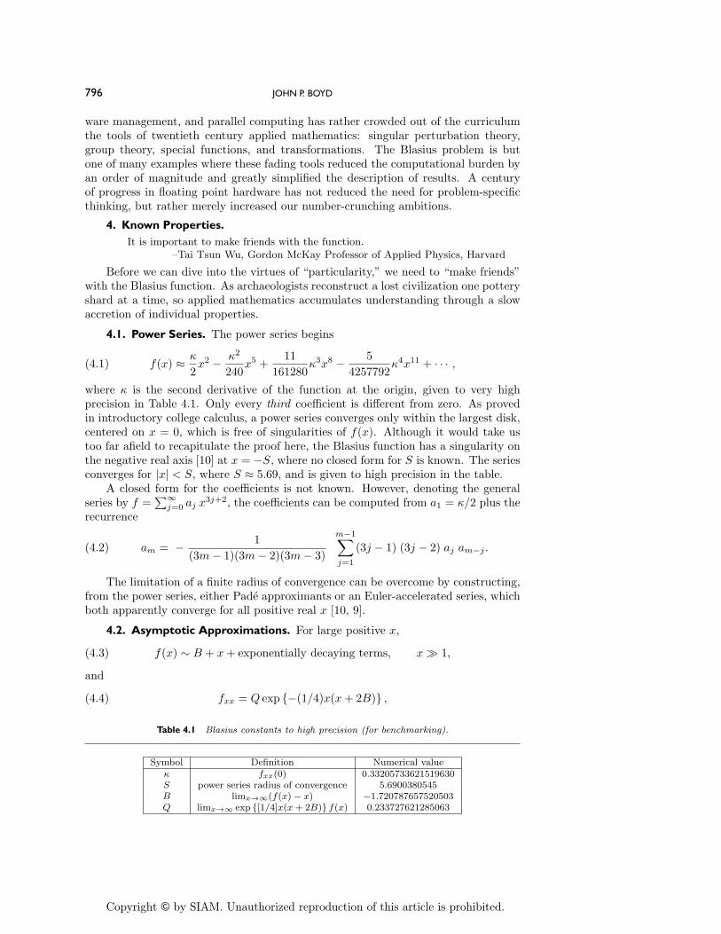
Fig. 4.1 The Blasius function in the complex plane. The coordinate is scaled by S, the distancefrom the origin to the nearest singularity. The three thick rays are the symmetry axesin the complex plane. The black dots denote known singularities of the Blasius function.The contours are the “equiconvergence” contours of the Euler-accelerated power series;everywhere along the contour labeled “0.8,” the n+ 1th term is smaller than the nth termby a factor of 0.8. The Eulerized series appears to converge everywhere within the regionbounded by the three dashed parabolas (including the entire positive real axis, which is thephysical domain for the flow), but a rigorous proof is lacking.
where Q ≈ 0.234 and B ≈ −1.72. (These constants are given to high precision inTable 4.1.)
The linear polynomial B+x, which is the leading order asymptotic approximationfor f(x), is an exact solution to the differential equation for all x, but fails to satisfy theboundary conditions. Physically, the Blasius velocity fx is constant at large distancesfrom the plate, and this implies that f(x) should asymptote to a linear function of xfar from the plate. Near the surface of the plate at x = 0, the streamfunction f curvesaway from the straight line to satisfy the boundary conditions at x = 0, creating aregion of rapid variation called a “boundary layer.”
4.3. Symmetry. The function fxx has a power series which contains every thirdpower of x. This implies that this function has a C3 symmetry in the complex plane.That is, fxx is the same on the rays arg = ±(2/3)π as on the positive real axis.Similarly, the singularity on the negative real x-axis which limits the convergence ofthe power series of f is replicated on the rays arg(x) = ±π/3. A contour plot of thefunction is unchanged by rotating it about the origin through any multiple of 120degrees, as in Figure 4.1. However, unlike the group invariances described earlier, theC3 complex plane symmetry does not simplify the problem.
However, because of this symmetry, the singularities of the Blasius function, de-scribed in the next subsection, must also always occur in threes: If there is a sin-gularity at x = ρ exp(iθ), then there must also be identical singularities at x =ρ exp(i[θ ± (2/3)π]).
4.4. Singularities. If we look for a singularity of the form
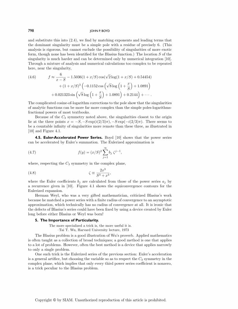
and substitute this into (2.4), we find by matching exponents and leading terms thatthe dominant singularity must be a simple pole with a residue of precisely 6. (Thisanalysis is rigorous, but cannot exclude the possibility of singularities of more exoticform, though none has been identified for the Blasius function.) The location S of thesingularity is much harder and can be determined only by numerical integration [10].Through a mixture of analysis and numerical calculations too complex to be repeatedhere, near the singularity,
The complicated cosine-of-logarithm corrections to the pole show that the singularitiesof analytic functions can be more far more complex than the simple poles-logarithms-fractional powers of most textbooks.
Because of the C3 symmetry noted above, the singularities closest to the originlie at the three points x = −S,−S exp(i(2/3)π),−S exp(−i(2/3)π). There seems tobe a countable infinity of singularities more remote than these three, as illustrated in[10] and Figure 4.1.
4.5. Euler-Accelerated Power Series. Boyd [10] shows that the power seriescan be accelerated by Euler’s summation. The Eulerized approximation is
(4.7) f(y) = (x/S)2∞∑j=1
bj ζj−1,
where, respecting the C3 symmetry in the complex plane,
(4.8) ζ ≡ 2x3
S3 + x3 ,
where the Euler coefficients bj are calculated from those of the power series aj bya recurrence given in [10]. Figure 4.1 shows the equiconvergence contours for theEulerized expansion.
Herman Weyl, who was a very gifted mathematician, criticized Blasius’s workbecause he matched a power series with a finite radius of convergence to an asymptoticapproximation, which technically has no radius of convergence at all. It is ironic thatthe defects of Blasius’s series could have been fixed by using a device created by Eulerlong before either Blasius or Weyl was born!
5. The Importance of Particularity.The more specialized a trick is, the more useful it is.
–Tai T. Wu, Harvard University lecture, 1973
The Blasius problem is a good illustration of Wu’s proverb. Applied mathematicsis often taught as a collection of broad techniques; a good method is one that appliesto a lot of problems. However, often the best method is a device that applies narrowlyto only a single problem.
One such trick is the Eulerized series of the previous section: Euler’s accelerationis a general artifice, but choosing the variable so as to respect the C3 symmetry in thecomplex plane, which implies that only every third power series coefficient is nonzero,is a trick peculiar to the Blasius problem.
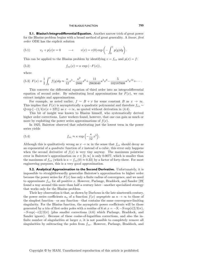
5.1. Blasius’s Integrodifferential Equation. Another narrow trick of great powerfor the Blasius problem begins with a broad method of great generality. A linear, firstorder ODE has the explicit solution
(5.1) vx + p(x)v = 0 −→ v(x) = v(0) exp(−∫ x
0p(y)dy
).
This can be applied to the Blasius problem by identifying v = fxx and p(x) = f :
(5.2) fxx(x) = κ exp (−F (x)) ,
where
(5.3) F (x) ≡ 12
∫ x
0f(y)dy ≈ κ
12x3− κ2
2880x6+
112903040
κ3x9− 5102187008
κ4x12+· · · .
This converts the differential equation of third order into an integrodifferentialequation of second order. By substituting local approximations for F (x), we canextract insights and approximations.
For example, as noted earlier, f ∼ B + x for some constant B as x → ∞.This implies that F (x) is asymptotically a quadratic polynomial and therefore fxx ∼Q exp {−(1/4)x(x+ 2B)} as x→∞, as quoted without derivation in (4.4).
This bit of insight was known to Blasius himself, who systematically derivedhigher order corrections. Later workers found, however, that one can gain as much ormore by exploiting the power series approximations of f(x).
In 1925, Bairstow observed that substituting just the lowest term in the powerseries yields
(5.4) fxx ≈ κ exp(− κ
12x3).
Although this is qualitatively wrong as x→∞ in the sense that fxx should decay asan exponential of a quadratic function of x instead of a cubic, this error only happenswhen the second derivative of f(x) is very tiny anyway. The maximum pointwiseerror in Bairstow’s approximation on x ∈ [0,∞] is only 0.0077, which is smaller thanthe maximum of fxx (which is κ = fxx(0) ≈ 0.33) by a factor of forty-three. For mostengineering purposes, this is a very good approximation.
5.2. Analytical Approximation to the Second Derivative. Unfortunately, it isimpossible to straightforwardly generalize Bairstow’s approximation to higher orderbecause the power series for F (x) has only a finite radius of convergence, and we needto approximate fxx for all positive x. However, Parlange, Braddock, and Sander [29]found a way around this more than half a century later—another specialized strategythat works only for the Blasius problem.
Their key observation is that, as shown by Darboux in the late nineteenth century,the power series coefficients an of a function f(x) asymptote as n → ∞ to those ofthe simplest function—or any function—that contains the same convergence-limitingsingularity. For the Blasius function, the asymptotic power coefficients will be thosegenerated by a trio of first order poles with a residue of 6 at x = −S,−S exp(i(2/3)π),−S exp(−i(2/3)π) (plus smaller corrections (4.6) which Parlange, Braddock, andSander ignore). Because of these cosine-of-logarithm corrections, and also the in-finite number of singularities at larger x, it is not possible to completely remove allsingularities by subtracting the poles from fxx. However, Parlange, Braddock, and
Sander realized that full singularity subtraction was unnecessary since Bairstow afterall obtained a decent approximation without even knowing the type or location of thesingularities!
The coefficients of f(x) are asymptotically those of
(5.5) σ(x) =18x2
184.2237031 + x3 ,
from whence it follows by integration that the coefficients of F (x) = (1/2)∫ x
Unlike F (y), the coefficients of Ξ(y) are known analytically as given in (5.10). Asymp-totically, Bn ∼ 3βn+1/(n+1), which are the power series coefficients of Ξ(y) displayedin (5.10).
Parlange, Braddock, and Sander’s idea is to rewrite F (x) by adding and subtract-ing Ξ—adding Ξ in its analytic, logarithmic form and subtracting Ξ in the form of itspower series truncated to the same number of terms as the series for F . Taking justthe first term gives
(5.11) F (x[y]) ≈ F (y) ≡ (1− .588496)y + 3 log(1 + βy),
(5.12) fxx(x[y]) =1
(1 + βy)3exp(−0.4115y).
The maximum absolute error on all x ∈ [0,∞] is 0.0013, which is an error relative toκ of less than 1 part in 250.
However, the power series expansion for F (y), which is
(5.13) F (y) ≈ y + 0.05772y2 + 0.007549y3 − 0.001111y4,
does not match the second term of the exact power series of F (y), which is
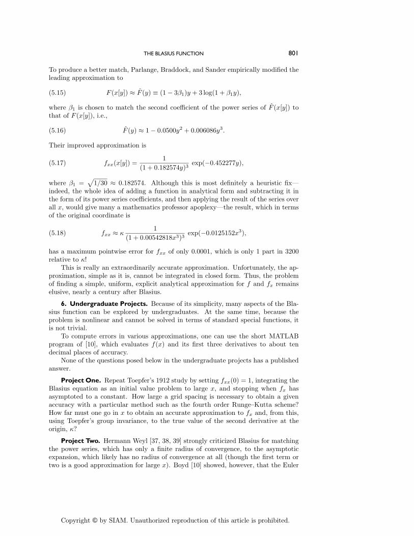
To produce a better match, Parlange, Braddock, and Sander empirically modified theleading approximation to
(5.15) F (x[y]) ≈ F (y) ≡ (1− 3β1)y + 3 log(1 + β1y),
where β1 is chosen to match the second coefficient of the power series of F (x[y]) tothat of F (x[y]), i.e.,
(5.16) F (y) ≈ 1− 0.0500y2 + 0.006086y3.
Their improved approximation is
(5.17) fxx(x[y]) =1
(1 + 0.182574y)3exp(−0.452277y),
where β1 =√1/30 ≈ 0.182574. Although this is most definitely a heuristic fix—
indeed, the whole idea of adding a function in analytical form and subtracting it inthe form of its power series coefficients, and then applying the result of the series overall x, would give many a mathematics professor apoplexy—the result, which in termsof the original coordinate is
(5.18) fxx ≈ κ1
(1 + 0.00542818x3)3exp(−0.0125152x3),
has a maximum pointwise error for fxx of only 0.0001, which is only 1 part in 3200relative to κ!
This is really an extraordinarily accurate approximation. Unfortunately, the ap-proximation, simple as it is, cannot be integrated in closed form. Thus, the problemof finding a simple, uniform, explicit analytical approximation for f and fx remainselusive, nearly a century after Blasius.
6. Undergraduate Projects. Because of its simplicity, many aspects of the Bla-sius function can be explored by undergraduates. At the same time, because theproblem is nonlinear and cannot be solved in terms of standard special functions, itis not trivial.
To compute errors in various approximations, one can use the short MATLABprogram of [10], which evaluates f(x) and its first three derivatives to about tendecimal places of accuracy.
None of the questions posed below in the undergraduate projects has a publishedanswer.
Project One. Repeat Toepfer’s 1912 study by setting fxx(0) = 1, integrating theBlasius equation as an initial value problem to large x, and stopping when fx hasasymptoted to a constant. How large a grid spacing is necessary to obtain a givenaccuracy with a particular method such as the fourth order Runge–Kutta scheme?How far must one go in x to obtain an accurate approximation to fx and, from this,using Toepfer’s group invariance, to the true value of the second derivative at theorigin, κ?
Project Two. Hermann Weyl [37, 38, 39] strongly criticized Blasius for matchingthe power series, which has only a finite radius of convergence, to the asymptoticexpansion, which likely has no radius of convergence at all (though the first term ortwo is a good approximation for large x). Boyd [10] showed, however, that the Euler
transformation of the power series appears to converge for all positive real x. (Thisis equivalent to making a conformal map of the complex x-plane and then computingthe power series of the transformed function.) The Euler transformation was knownin 1908 and thus could have been applied by Blasius himself. “Rehabilitate” thepower series by examining the convergence of the Euler-accelerated expansion. Canone obtain accurate values for κ from the Eulerized power series alone? (Boyd [10]does a similar analysis for another method of series extension known in 1908, Padeapproximation. However, Euler’s method is much better suited to hand computation,and would have been Blasius’ preferred choice.)
Project Three. The power series coefficients of a function with a simple pole are
(6.1)r
1 + x/S= r
∞∑n=0
(−1)N 1Sn
xn,
where S is a constant which is also the radius of convergence of the series. What arethe power series coefficients for a singularity of the form of the second worst singularitythat appears in the Blasius function,
(6.2) h(x) ≡ (1 + x) cos(log(1 + x)) =∞∑n=0
hnxn?
Why is there no loss of generality in placing the singularity at x = −1?It is easy to observe, by using the command for computing a power series in Maple
or Mathematica or a similar symbolic manipulation system, that hn decreases roughlyas 1/n2. Can one be more precise?
7. Open Research Problems. Although the Blasius problem is simple enoughfor fooling around with by undergraduates, it still poses unresolved challenges for theresearch mathematician. A few of these include the following, some from [10].
1. A proof that the Eulerized power series converges for all positive real x(strongly supported by numerical evidence).
2. A proof that diagonal Pade approximations converge for all positive real x(strongly supported by numerical evidence).
3. A proof that f(x) is free of singularities everywhere in the sector arg(x) ≤π/4 (supported by the asymptotic approximation, which is accurate andsingularity-free in this sector).
4. A rigorous and complete analysis of the essential singularities that are super-imposed upon the simple pole at x = −5.69.
5. A simple, uniformly accurate analytical approximation to f(x), similar tothat already known for fxx.
6. A theory for the asymptotic approximation of the power series coefficients forfunctions with singularities of the form (1 + x) cos(log(1 + x)), as occurs inthe Blasius function.
8. Summary. One maxim for good number-crunching is: Never solve a PDEwhen an ODE will do, and never solve a boundary value problem when an initialvalue problem will do. Blasius and Toepfer successfully applied this maxim usingmathematical tools which students are no longer taught very often. The film directorSir Alfred Hitchcock said his most important and enjoyable work was all done beforefilming even began: the meticulous planning of each shot in his mind. Similarly,the most important part of computing is what happens before the code is written.
Numerical analysis classes do a good job of explaining the importance of choosingan efficient numerical scheme. They do not usually do a good job of explaining thenonnumerical Blasius-and-Toepfer-like “precomputing.”
The second theme is that many problems can be attacked with special tricks. Thisruns counter to the ever-generalize, even-more-abstract prevalent trend of pure math-ematics. In contrast, applied mathematicians are plumbers, always adapting generalstrategies, like copper pipes and traps and plumber’s putty, to the idiosyncrasies ofthe problem at hand, never too proud to hammer a pipe into alignment, never tooproud to use a trick that only works for a narrow, specific problem.
The third theme is that even though the Blasius function has been intensivelystudied for a century, there are still many challenging open problems at all levels:some that are educational fun for an undergraduate, others that test the skills of apostdoctoral mathematician. The high school treatment of the “scientific method” asa sequence of ever-more-complex problems, vanquished and left behind, is unrealistic.The history of the Blasius problem is more typical: a major problem is never com-pletely solved. Instead, science is like lunar exploration: we return again and againwith different satellites and landers, slowly making the map of knowledge denser.
Acknowledgments. I thank the reviewers for helpful comments and Louis F.Rossi for his thoughtful editing.
REFERENCES
[1] F. M. Allan and M. I. Syam, On the analytic solutions of the nonhomogeneous Blasiusproblem, J. Comput. Appl. Math., 182 (2005), pp. 362–371.
[2] A. Arikoglu and I. Ozkol, Inner-outer matching solution of Blasius equation by DTM,Aircraft Engrg. Aero. Tech., 77 (2005), pp. 298–301.
[3] W. Aspray, ed., Computing Before Computers, Iowa State University Press, Ames, Iowa,1990.
[4] F. Bashforth and J. C. Adams, Theories of Capillary Action, Cambridge University Press,London, 1883.
[5] C. M. Bender, A. Pelster, and F. Weissbach, Boundary-layer theory, strong-coupling se-ries, and large-order behavior, J. Math. Phys., 43 (2002), pp. 4202–4220.
[6] N. Bildik and A. Konuralp, The use of variational iteration method, differential transformmethod and Adomian decomposition method for solving different types of nonlinear partialdifferential equations, Internat. J. Nonlinear Sci. Numer. Simul., 7 (2006), pp. 65–70.
[7] H. Blasius, Grenzschichten in flussigkeiten mit kleiner reibung, Zeit. Math. Phys., 56 (1908),pp. 1–37.
[8] G. Boole, A Treatise on the Calculus of Finite Differences, 1st ed., Macmillan, Cambridge,UK, 1860.
[9] J. P. Boyd, Pade approximant algorithm for solving nonlinear ODE boundary value problemson an unbounded domain, Computers and Phys., 11 (1997), pp. 299–303.
[10] J. P. Boyd, The Blasius function in the complex plane, J. Experimental Math., 8 (1999),pp. 381–394.
[11] R. Cortell, Numerical solutions of the classical Blasius flat-plate problem, Appl. Math. Com-put., 170 (2005), pp. 706–710.
[12] M. Croarken, Early Scientific Computing in Britain, Oxford University Press, Oxford, 1990.[13] M. Croarken, R. Flood, E. Robson, and M. Campbell-Kelly, The History of Mathematical
Tables: From Sumer to Spreadsheets, Oxford University Press, Oxford, 2003.[14] G. H. Darwin, Periodic orbits, Acta Math., 21 (1897), pp. 99–242.[15] B. K. Datta, Analytic solution for the Blasius equation, Indian J. Pure Appl. Math., 34 (2003),
pp. 237–240.[16] T. G. Fang and C. F. E. Lee, A moving-wall boundary layer flow of a slightly rarefied gas
free stream over a moving flat plate, Appl. Math. Lett., 18 (2005), pp. 487–495.[17] R. Fazio, The Blasius problem formulated as a free-boundary value problem, Acta Mech., 95
[18] R. Fazio, A similarity approach to the numerical solution of free boundary problems, SIAMRev., 40 (1998), pp. 616–635.
[19] C. W. Gear and R. Skeel, The development of ODE methods: A symbiosis between hardwareand numerical analysis, in History of Scientific and Numerical Computation: Proceedingsof the ACM Conference on History of Scientific and Numerical Computation, Princeton,NJ, 1987, ACM, New York, 1987, pp. 105–115.
[20] D. A. Grier, When Computers Were Human, Princeton University Press, Princeton, NJ, 2005.[21] J. H. He, A simple perturbation approach to Blasius equation, Appl. Math. Comput., 140
(2003), pp. 217–222.[22] L. Howarth, On the solution of the laminar boundary equations, Proc. R. Soc. London Ser.
A, 164 (1938), pp. 547–579.[23] I. K. Khabibrakhmanov and D. Summers, The use of generalized Laguerre polynomials in
[24] C. Lanczos, Trigonometric interpolation of empirical and analytical functions, J. Math. Phys.,17 (1938), pp. 123–199; reprinted in Cornelius Lanczos: Collected Papers with Commen-taries, Vol. 3, W. R. Davis et al., eds., North Carolina State University, 1997, pp. 221–297.
[25] S. J. Liao, An explicit, totally analytic approximate solution for Blasius’ viscous flow problems,Internat. J. Nonlinear Mech., 34 (1999), pp. 759–778.
[26] S. J. Liao, A uniformly valid analytic solution of two-dimensional viscous flow over a semi-infinite flat plate, J. Fluid Mech., 385 (1999), pp. 101–128.
[27] S. J. Liao, A non-iterative numerical approach for two-dimensional viscous flow problemsgoverned by the Falkner–Skan equation, Internat. J. Numer. Meths. Fluids, 35 (2001),pp. 495–518.
[28] G. R. Liu and T. Y. Wu, Application of generalized differential quadrature rule in Blasiusand Onsager equations, Internat. J. Numer. Methods Engrg., 52 (2001), pp. 1013–1027.
[29] J. Parlange, R. D. Braddock, and G. Sander, Analytical approximations to the solution ofthe Blasius equation, Acta Mech., 38 (1981), pp. 119–125.
[30] L. Roman-Miller and P. Broadbridge, Exact integration of reduced Fisher’s equation, re-duced Blasius equation, and the Lorenz model, J. Math. Anal. Appl., 251 (2000), pp. 65–83.
[31] L. Rosenhead, The formation of vortices from a surface of discontinuity, Proc. R. Soc. LondonSer. A, 134 (1931), pp. 170–192.
[32] A. A. Salama and A. A. Mansour, Higher-order method for solving free boundary-valueproblems, Numer. Heat Transfer. Part B: Fundamentals, 45 (2004), pp. 385–394.
[33] A. A. Salama and A. A. Mansour, Finite-difference method of order six for the two-dimensional steady and unsteady boundary-layer equations, Internat. J. Modern Phys. C,16 (2005), pp. 757–780.
[34] A. A. Salama and A. A. Mansour, Fourth-order finite-difference method for third-orderboundary-value problems, Numer. Heat Transfer. Part B: Fundamentals, 47 (2005), pp. 383–401.
[35] K. Topfer, Bemerkung zu dem Aufsatz von H. Blasius “Grenzschichten in Flussigkeiten mitkleiner Reibung,” Zeit. Math. Phys., 60 (1912), pp. 397–398.
[36] L. Wang, A new algorithm for solving classical Blasius equation, Appl. Math. Comput., 157(2004), pp. 1–9.
[37] H. Weyl, Concerning the differential equations of some boundary layer problems, Proc. Natl.Acad. Sci., 27 (1941), pp. 578–583.
[38] H. Weyl, Concerning the differential equations of some boundary layer problems, Proc. Natl.Acad. Sci., 28 (1942), pp. 100–101.
[39] H. Weyl, On the differential equations of the simplest boundary-layer problems, Ann. Math.,43 (1942), pp. 381–407.