Numerical studies of bypass transition in the Blasius ...9331/FULLTEXT01.pdf · Numerical studies...

Numerical studies of bypass transition

in the Blasius boundary layer.

by

Luca Brandt

April 2003Technical Reports from

Royal Institute of TechnologyDepartment of Mechanics

SE-100 44 Stockholm, Sweden

Typsatt i AMS-LATEX.

Akademisk avhandling som med tillstand av Kungliga Tekniska Hogskolan iStockholm framlagges till offentlig granskning for avlaggande av teknologiedoktorsexamen tisdagen den 20:e maj 2003 kl 10.15 i Kollegiesalen, Admin-istrationsbyggnaden, Kungliga Tekniska Hogskolan, Valhallavagen 79, Stock-holm.

c©Luca Brandt 2003

Universitetsservice AB, Stockholm 2003

Numerical studies of bypass transition in the Blasius boundarylayer.

Luca Brandt 2003Department of Mechanics, Royal Institute of TechnologySE-100 44 Stockholm, Sweden.

AbstractExperimental findings show that transition from laminar to turbulent flow

may occur also if the exponentially growing perturbations, eigensolutions tothe linearised disturbance equations, are damped. An alternative non-modalgrowth mechanism has been recently identified, also based on the linear ap-proximation. This consists of the transient growth of streamwise elongateddisturbances, with regions of positive and negative streamwise velocity alter-nating in the spanwise direction, called streaks. These perturbation are seento appear in boundary layers exposed to significant levels of free-stream tur-bulence. The effect of the streaks on the stability and transition of the Blasiusboundary layer is investigated in this thesis. The analysis considers the steadyspanwise-periodic streaks arising from the nonlinear evolution of the initialdisturbances leading to the maximum transient energy growth. In the absenceof streaks, the Blasius profile supports the viscous exponential growth of theTollmien-Schlichting waves. It is found that increasing the streak amplitudethese two-dimensional unstable waves evolve into three-dimensional spanwise-periodic waves which are less unstable. The latter can be completely stabilisedabove a threshold amplitude. Further increasing the streak amplitude, theboundary layer is again unstable. The new instability is of different character,being driven by the inflectional profiles associated with the spanwise modu-lated flow. In particular, it is shown that, for the particular class of steadystreaks considered, the most amplified modes are antisymmetric and lead tospanwise oscillations of the low-speed streak (sinuous scenario). The transi-tion of the streak is then characterised by the appearance of quasi-streamwisevortices following the meandering of the streak.

Simulations of a boundary layer subjected to high levels of free-streamturbulence have been performed. The receptivity of the boundary layer to theexternal perturbation is studied in detail. It is shown that two mechanisms areactive, a linear and a nonlinear one, and their relative importance is discussed.The breakdown of the unsteady asymmetric streaks forming in the boundarylayer under free-stream turbulence is shown to be characterised by structuressimilar to those observed both in the sinuous breakdown of steady streaks andin the varicose scenario, with the former being the most frequently observed.

Descriptors: Fluid mechanics, laminar-turbulent transition, boundary layerflow, transient growth, streamwise streaks, lift-up effect, receptivity, free-streamturbulence, secondary instability, Direct Numerical Simulation.

Preface

This thesis considers the study of bypass transition in a zero-pressure-gradientboundary layer. The first part is a summary of the research presented in thepapers included in the second part. The summary includes an introduction tothe basic concept, a review of previous works and a presentation and discussionof the main results obtained.

The thesis is based on and contains the following papers.

Paper 1. Andersson, P., Brandt, L., Bottaro, A. & Henningson,

D. S. 2001 On the breakdown of boundary layer streaks. Journal of FluidMechanics , 428, pp. 29-60.

Paper 2. Brandt, L., Cossu, C., Chomaz, J.-M., Huerre, P. & Hen-

ningson, D. S. 2003 On the convectively unstable nature of optimal streaksin boundary layers. Journal of Fluid Mechanics , In press.

Paper 3. Brandt, L. & Henningson, D. S. 2002 Transition of streamwisestreaks in zero-pressure-gradient boundary layers. Journal of Fluid Mechanics ,472, pp. 229-262.

Paper 4. Cossu, C. & Brandt, L. 2002 Stabilization of Tollmien-Schlichtingwaves by finite amplitude optimal streaks in the Blasius boundary layer. Physicsof Fluids , 14, pp. L57-L60.

Paper 5. Cossu, C. & Brandt, L. 2003 On the stabilizing role of boundarylayer streaks on Tollmien-Schlichting waves.

Paper 6. Brandt, L., Henningson, D. S., & Ponziani D. 2002 Weaklynon-linear analysis of boundary layer receptivity to free-stream disturbances.Physics of Fluids, 14, pp. 1426-1441.

Paper 7. Brandt, L., Schlatter, P. & Henningson, D. S. 2003 Boundary-layer transition under free-stream turbulence.

PREFACE v

Division of work between authors

The Direct Numerical Simulations (DNS) were performed with a numericalcode already in use mainly for transitional research, developed originally byAnders Lundbladh, Dan Henningson (DH) and Arne Johansson. It is based ona pseudo-spectral technique and has been further developed by several users,including Luca Brandt (LB) for generating new inflow conditions and extractingflow quantities needed during the work.

The DNS data and secondary instability calculations presented in Paper 1were done by LB, who also collaborated in the writing process. The theoryand the writing was done by Paul Andersson, Alessandro Bottaro and DH.The simulations presented in Paper 2 were performed by LB with help fromCarlo Cossu (CC). The writing was done by LB and Patrick Huerre, withfeedback from J.-M. Chomaz and DH. The DNS in Paper 3 were performed byLB. The writing was done by LB with help from DH.

The simulations presented in Paper 4 were performed by CC and LB. Thepaper was written by CC with help from LB. The numerical code for thestability calculations in Paper 5 was implemented by CC, who also carried outthe computations. The paper was written by CC with help from LB.

The numerical implementation of the perturbation model presented in Pa-per 6 was done in collaboration between LB and Donatella Ponziani (DP). Thewriting was done by LB and DP with help from DH.

The turbulent inflow generation used in Paper 7 was implemented byPhilipp Schlatter (PS) with help from LB and DH. The simulation were carriedout by PS and LB. The paper was written by LB with help from PS and DH.

Contents

Preface iv

Chapter 1. Introduction 1

Chapter 2. Transition in Blasius boundary layers 42.1. Natural transition 42.2. Bypass transition 5

Chapter 3. Direct numerical simulations 83.1. Numerical method 83.2. Disturbance generation 10

Chapter 4. Instability and breakdown of steady optimal streaks 124.1. Steady saturated streaks 124.2. Streak instability 14

4.2.1. Viscous instabilities in low-amplitude streaks 184.2.2. Inviscid instability 214.2.3. Spatio-temporal behaviour 22

4.3. Streak breakdown 26

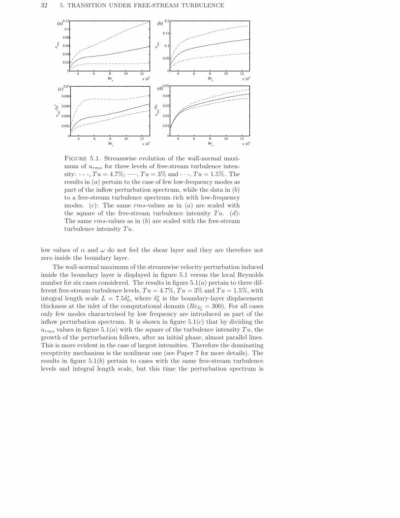
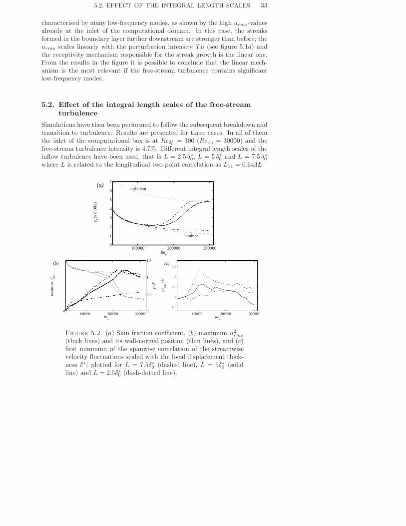
Chapter 5. Transition in boundary layers subjected to free-stream turbulence 30

5.1. Receptivity 305.2. Effect of the integral length scales of the free-stream turbulence 335.3. Turbulent spot generation 34

Chapter 6. Conclusions and outlook 38

Acknowledgment 41

Bibliography 42

Part 2. Papers 47

vii

viii CONTENTS

Paper 1. On the breakdown of boundary layer streaks 51

Paper 2. On the convectively unstable nature of optimalstreaks in boundary layers 93

Paper 3. Transition of streamwise streaks in zero-pressure-gradient boundary layers 123

Paper 4. Stabilization of Tollmien-Schlichting waves by finiteamplitude optimal streaks in the Blasius boundarylayer 167

Paper 5. On the stabilizing role of boundary layer streaks onTollmien-Schlichting waves 177

Paper 6. Weakly nonlinear analysis of boundary layer receptivityto free-stream disturbances 211

Paper 7. Boundary-layer transition under free-streamturbulence 245

CHAPTER 1

Introduction

The motion of a fluid is usually defined as laminar or turbulent. A laminarflow is an ordered, predictable and layered flow (from Latin “lamina”: layer,sheet, leaf) as opposed to the chaotic, swirly and fluctuating turbulent flow.In a laminar flow the velocity gradients and the shear stresses are smaller;consequently the drag force over the surface of a vehicle is much lower than ina turbulent flow. One of the major challenges in aircraft design is in fact toobtain a laminar flow over the wings to reduce the friction in order to save fuel.On the other hand a turbulent flow provides an excellent mixing in the flowbecause of the chaotic motion of the fluid particles, and it is therefore requiredin chemical reactors or combustion engines.

In real applications, as the velocity of the fluid or the physical dimensionlimiting the flow increase, a laminar motion cannot be sustained; the pertur-bations inevitably present within the flow are amplified and the flow evolvesinto a turbulent state. This phenomenon is called transition.

Transition and its triggering mechanisms are today not fully understood,even though the first studies on this field dates back to the end of the nineteenthcentury. The very first piece of work is traditionally considered the classicalexperiment of Osborne Reynolds in 1883 performed at the hydraulics laboratoryof the Engineering Department at Manchester University. Reynolds studiedthe flow inside a glass tube injecting ink at the centreline of the pipe inlet.If the flow stayed laminar, he could observe a straight coloured line insidethe tube. When transition occurred, the straight line became irregular andthe ink diffused all over the pipe section. He found that the value of a nondimensional parameter, later called Reynolds number, Re = Ur

ν , where U isthe bulk velocity, r the pipe radius and ν the kinematic viscosity, governedthe passage from the laminar to the turbulent state. This non dimensionalparameter relates the inertial effects to the viscous forces acting on the movingfluid particles. The two latter forces are therefore the only involved in thephenomenon under consideration. Reynolds stated quite clearly, however, thatthere is no a single critical value of the parameter Re, above which the flowbecomes unstable and transition may occur; the whole matter is much morecomplicated. He noted the sensitivity of the transition to disturbances in theflow before entering the tube. For large disturbances at the pipe inlet, in fact,the flow became unstable at lower critical velocities and the chaotic motionappeared intermittently for short distances, like flashes, along the pipe.

1

2 1. INTRODUCTION

y

v

u

x

w z

U

U∞

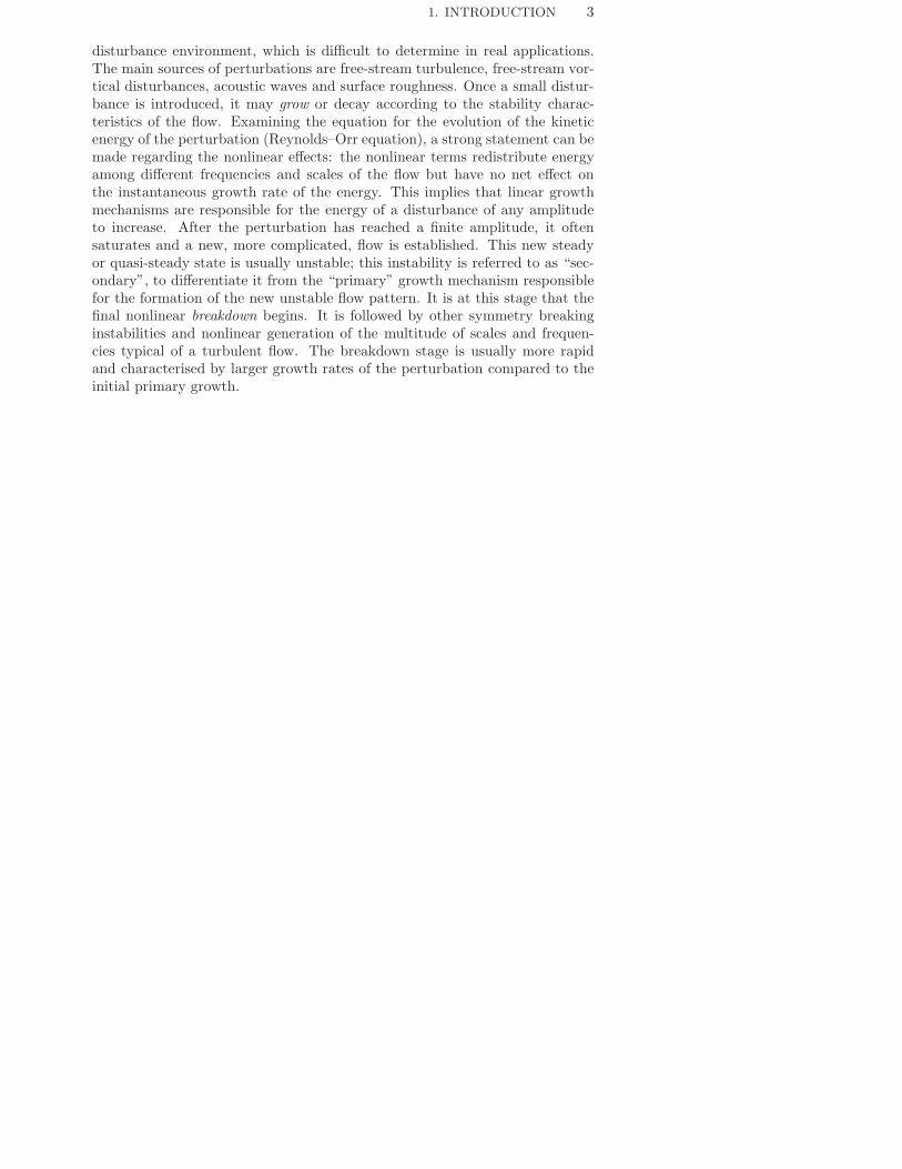
Figure 1.1. Boundary layer flow with free-stream velocityU∞. The velocity has components u, v and w in the coordinatesystem x, y and z.

The knowledge of why, where and how a flow becomes turbulent is of greatpractical importance in almost all the application involving flows either internalor external; therefore there is a need to improve the models able to predict thetransition onset currently available. In gas turbines, where a turbulent freestream is present, the flow inside the boundary layer over the surface of a bladeis transitional for 50 − 80% of the chord length. Wall shear stresses and heattransfer rates are increased during transition and a correct design of the thermaland shear loads on the turbine blades must take into account the features ofthe transitional process.

The present thesis deals with transition in the simplified case of the bound-ary layer over a flat plate subject to a uniform oncoming flow. The friction atthe wall will slow down the fluid particles; due to viscosity the velocity of theflow will vary from the free-stream value a distance above the wall (boundarylayer thickness) to zero at the plate surface, with the thickness growing as theflow evolves downstream, see figure 1.1. This flow is also referred to as Blasiusboundary layer after the scientist who, under certain assumptions, solved thegoverning fluid dynamics equations (Navier–Stokes equations) for this partic-ular configuration. This is one of the simplest configurations, but still helpsus to gain some physical insight in the transition process. It has been in factobserved that independently of the background disturbances and environmentthe flow eventually becomes turbulent further downstream. The backgroundenvironment determines, however, the route the transition process will followand the location of its onset. Other effects present in real applications suchas curvature of the surface or pressure gradients, which give an accelerating ordecelerating flow outside the boundary layer, will not be considered.

The transition process may be divided into three stages: receptivity, dis-turbance growth and breakdown. In the receptivity stage the disturbance isinitiated inside the boundary layer. This is the most difficult phase of the fulltransition process to predict because it requires the knowledge of the ambient

1. INTRODUCTION 3

disturbance environment, which is difficult to determine in real applications.The main sources of perturbations are free-stream turbulence, free-stream vor-tical disturbances, acoustic waves and surface roughness. Once a small distur-bance is introduced, it may grow or decay according to the stability charac-teristics of the flow. Examining the equation for the evolution of the kineticenergy of the perturbation (Reynolds–Orr equation), a strong statement can bemade regarding the nonlinear effects: the nonlinear terms redistribute energyamong different frequencies and scales of the flow but have no net effect onthe instantaneous growth rate of the energy. This implies that linear growthmechanisms are responsible for the energy of a disturbance of any amplitudeto increase. After the perturbation has reached a finite amplitude, it oftensaturates and a new, more complicated, flow is established. This new steadyor quasi-steady state is usually unstable; this instability is referred to as “sec-ondary”, to differentiate it from the “primary” growth mechanism responsiblefor the formation of the new unstable flow pattern. It is at this stage that thefinal nonlinear breakdown begins. It is followed by other symmetry breakinginstabilities and nonlinear generation of the multitude of scales and frequen-cies typical of a turbulent flow. The breakdown stage is usually more rapidand characterised by larger growth rates of the perturbation compared to theinitial primary growth.

CHAPTER 2

Transition in Blasius boundary layers

2.1. Natural transition

Historically, the first approach to transition was the analysis of the stability ofa flow. Equations for the evolution of a disturbance, linearised around a meanvelocity profile were first derived by Lord Rayleigh (1880) for an inviscid flow.He considered a two-dimensional basic flow consisting only of the streamwisevelocity component assumed to vary only in one cross-stream direction (paral-lel flow assumption). Assuming a wave–like form of the velocity perturbationand Fourier transforming the equation, it reduces to an eigenvalue problem forexponentially growing or decaying disturbances. From this equation, Rayleighproved his inflection point theorem which states that a necessary condition forinviscid instability is the presence of an inflection point in the basic velocityprofile. Later Orr (1907) and Sommerfeld (1908) included the effects of viscos-ity, deriving independently what we today call the Orr–Sommerfeld equation.The latter is an equation for the wall-normal component of the perturbationvelocity and it suffices to describe the evolution of two-dimensional disturban-ces. To describe three-dimensional perturbation one more equation is needed;for this, an equation for the wall-normal vorticity is commonly used (Squireequation). The first solutions for two-dimensional unstable waves in the Bla-sius boundary layer were presented by Tollmien (1929) and Schlichting (1933).The existence of such solutions (TS-waves) was experimentally shown to existby Schubauer & Skramstad (1947).

About at the same time, Squire’s theorem (1933), stating that two dimen-sional waves are the first to become unstable, directed the early studies onstability towards two-dimensional perturbations. The stability of such eigen-modes of the Orr–Sommerfeld problem depends on their wavelength, frequency,and on the Reynolds number, defined for a boundary later flow as Re = U∞δ

ν ,with δ =

√(xν/U∞) the boundary layer thickness. Since δ is increasing in the

downstream direction, see figure 1.1, the Reynolds number varies and the TS-waves growth rate is also function of the downstream position along the plate.The classical stability theory assumes that the boundary layer has a constantthickness, the so called parallel flow assumption. The stability of a distur-bance is evaluated for different Reynolds numbers, mimicking the downstreamevolution of the Blasius flow. This proved to be a reasonable approximation(Fasel & Konzelman 1990; Klingmann et al. 1993), even if different models

4

2.2. BYPASS TRANSITION 5

have been now developed to include the boundary layer growth in the stabilitycalculations (see for example the Parabolized Stability Equations introducedby Herbert & Bertolotti 1987).

If an amplified Tollmien–Schlichting wave grows above an amplitude inurms of 1% of the free-stream velocity, the flow become susceptible to sec-ondary instability. Klebanoff, Tidstrom & Sargent (1962) observed that three-dimensional perturbations, which are present in any natural flow, were stronglyamplified. The three-dimensional structure of the flow was characterised by re-gions alternating in the spanwise direction of enhanced and diminished pertur-bation velocity amplitudes, denoted by them “peaks and valleys”. The spanwisescale of the new pattern was of the same order of the streamwise wavelengthof the TS-waves and the velocity time signal showed the appearance of highfrequency disturbance spikes at the peak position. This transition scenariowas later denoted as K-type after Klebanoff but also fundamental since thefrequency of the secondary, spanwise periodic, fluctuations is the same as theone of the TS-waves. In the non-linear stages of the K-type scenario, rows of“Λ-shaped” vortices, aligned in the streamwise directions, have been observed.An other scenario was also observed, first by Kachanov, Kozlov & Levchenko(1977). This is denoted N-type after Novosibirsk, where the experiments werecarried out or H-type after Herbert, who performed a theoretical analysis ofthe secondary instability of TS-waves (Herbert 1983). In this scenario, thefrequency of the secondary instability mode is half the one of the TS-wavesand, thus, this is also known as subharmonic breakdown. “Λ-shaped” vorticesare present also in this case, but they are arranged in a staggered pattern.Experiments and computations reveals that the N-type scenario is the first tobe induced, when small three-dimensional perturbations are forced in the flow.

Transition originating from exponentially growing eigenfunctions is usuallycalled classical or natural transition. This is observed in natural flows onlyif the background turbulence is very small; as a rule of thumb it is usuallyassumed that natural transition occurs for free-stream turbulence levels lessthan 1%. For higher values, the disturbances inside the boundary layer arelarge enough that other mechanisms play an important role and the naturalscenario is bypassed.

2.2. Bypass transition

In 1969 Morkovin coined the expression “bypass transition”, noting that “wecan bypass the TS-mechanism altogether”. In fact, experiments reveal thatmany flows, including channel and boundary layer flows, may undergo tran-sition for Reynolds numbers well below the critical ones from linear stabilitytheory. The first convincing explanation for this was proposed by Ellingsen& Palm (1975). They considered, in the inviscid case, an initial disturbanceindependent of the streamwise coordinate in a shear layer and showed that thestreamwise velocity component may grow linearly in time, producing alternat-ing low- and high-velocity streaks. Hultgren & Gustavsson (1981) considered

6 2. TRANSITION IN BOUNDARY LAYERS

the temporal evolution of a three-dimensional disturbance in a boundary layerand found that in a viscous flow the initial growth is followed by a viscousdecay (transient growth).

Landahl (1975) proposed a physical explanation for this growth. A wall-normal displacement of a fluid element in a shear layer will cause a perturbationin the streamwise velocity, since the fluid particle will initially retain its hor-izontal momentum. As a consequence, since weak pairs of quasi streamwisecounter rotating vortices are able to lift up fluid with low velocity from thewall and bring high speed fluid towards the wall, they are the most effective inforcing streamwise oriented streaks of high and low streamwise velocity, alter-nating in the spanwise direction. This mechanism is denoted lift-up effect andit is inherently a three-dimensional phenomenon. Some insight in it may alsobe gained from the equation for the wall-normal vorticity of the perturbation(Squire equation), which is proportional to the streamwise velocity for stream-wise independent disturbances. The equation is, in fact, forced by a term dueto the interaction between the spanwise variation of the wall-normal velocityperturbation and the mean shear of the base flow.

From a mathematical point of view, it is now clear that since the linearisedNavier–Stokes operator is non-normal for many flow cases (e.g. shear flows),a significant transient growth may occur before the subsequent exponentialbehaviour (see Schmid & Henningson 2001). Such growth is larger for distur-bances mainly periodic in the spanwise direction, that is with low frequency orstreamwise wave numbers; it can exist for sub-critical values of the Reynoldsnumber and it is the underlying mechanism in bypass transition phenomena.In particular, for the Blasius boundary layer, Andersson, Berggren & Henning-son (1999) and Luchini (2000) used an optimisation technique to determinewhich disturbance present at the leading edge gives the largest disturbance inthe boundary layer. This optimal perturbation was found to consist of a pairof steady streamwise counter-rotating vortices, which induce strong streamwisestreaks.

For real applications, the most interesting case in which disturbances orig-inating from non-modal growth are responsible for transition, is probably inthe presence of free-stream turbulence. Inside the boundary layer in fact, theturbulence is highly damped, but low frequency oscillations, associated withlong streaky structures, appear. The first experimental study of such distur-bances is due to Klebanoff (1971). Arnal & Juillen (1978) also showed thatfor free-stream turbulence levels higher than 0.5–1%, the dominant disturban-ces inside the boundary layer are characterised by low frequencies and theyare not TS-waves. Kendall (1985) denoted these disturbances as Klebanoffmodes. As the streaks grow downstream, they breakdown into regions of in-tense randomised flow, turbulent spots. The leading edge of these spots travelsat nearly the free-stream velocity, while the trailing edge at about half of thespeed; thus a spot grows in size and merges with other spots until the flow iscompletely turbulent. Westin et al. (1994) presented detailed measurements

2.2. BYPASS TRANSITION 7

of a laminar boundary layer subjected to free-stream turbulence and showedhow different experiments with apparently similar conditions can disagree onthe location and extent of transition. A recent review on the experimentalstudies of boundary-layer transition induced by free-stream turbulence can befound in Matsubara & Alfredsson (2001), while the first numerical simulationsare presented in Jacobs & Durbin (2001). This scenario is usually observed forhigh levels of free-stream turbulence and transition occurs at Reynolds numberslower than in the case of natural transition.

An other case where transient growth plays an important role is in theso called oblique transition. In this scenario, streamwise aligned vortices aregenerated by non-linear interaction between a pair of oblique waves with equalangle but opposite sign in the flow direction. These vortices, in turn, inducestreamwise streaks, which may grow over a certain amplitude and become un-stable, initiating the breakdown to a turbulent flow. Oblique transition hasbeen studied in detail both numerically and experimentally by Berlin, Wiegel& Henningson (1999).

Transition to turbulence may, thus, follow different routes, according tothe disturbance environment. In general, as soon as streamwise vortices arepresent in the flow, strong streamwise streaks are created, and the breakdown toturbulence occurs through their growth and breakdown. In this thesis, bypasstransition is analysed; first, the instability and breakdown of steady, spanwiseperiodic streaks is studied as a model problem to understand the mechanismsinvolved in the scenario under consideration. The results are then applied to thecase of a boundary layer subject to high levels of free-stream turbulence. Thedifferent approaches used and the main results obtained are shortly summarisedin the next chapters.

CHAPTER 3

Direct numerical simulations

3.1. Numerical method

Most of the results presented in this thesis have been obtained by means of di-rect numerical simulations (DNS). That is, the temporal and spatial evolutionof the flow is obtained by numerical solution of the governing Navier-Stokesequations without any simplifying assumptions. This requires larger computa-tional efforts, both in term of memory and effective time of the calculations,since all the relevant scales characterising the flow configuration under exami-nation must be resolved.

The rapid development of fast parallel computers in recent years has pro-vided the scientific community with the possibility of simulating fully turbulentflows. A clear advantage is that, once a flow is simulated, it is completely acces-sible to observation including three-dimensional views and derived quantitieswhich are usually impossible to obtain in an experiment. Also important is thepossibility of simulating ’unphysical’ flows, obtained by equations and bound-ary conditions which differ from the real ones, so as to allow us to study partialprocesses, to verify hypothetical mechanisms or to test possible control strate-gies. The numerical simulation has lead to important improvements of ourphysical understanding of transitional and turbulent flows, especially on thedynamics of flow structures. However, in the case of turbulent flows the simu-lations are limited to Reynolds number lower than those of typical applications.The available computational resources may also limit the physical dimensionof the computational domain, leading to crucial choices of the boundary condi-tions. On the other hand, experiments allow to study larger Reynolds numberand more complicated geometries. In a experiment, it is also simpler to per-form a parametric study; once the set-up is validated, it is relatively cheaperto perform a new experiment than a completely new simulation.

The direct numerical simulations presented in this thesis have all beenperformed with the pseudo-spectral algorithm described in Lundbladh et al.(1999). In spectral methods the solution is approximated by an expansionin smooth functions, trigonometric functions and Chebyshev polynomials inour case. The earliest applications to partial differential equations were devel-oped by Kreiss & Oliger (1972) and Orszag (1972), who also introduced thepseudo-spectral approach. In this, the multiplications of the nonlinear termsare calculated in physical space to avoid the evaluation of convolution sums.

8

3.1. NUMERICAL METHOD 9

δ

λ(x)

��

��

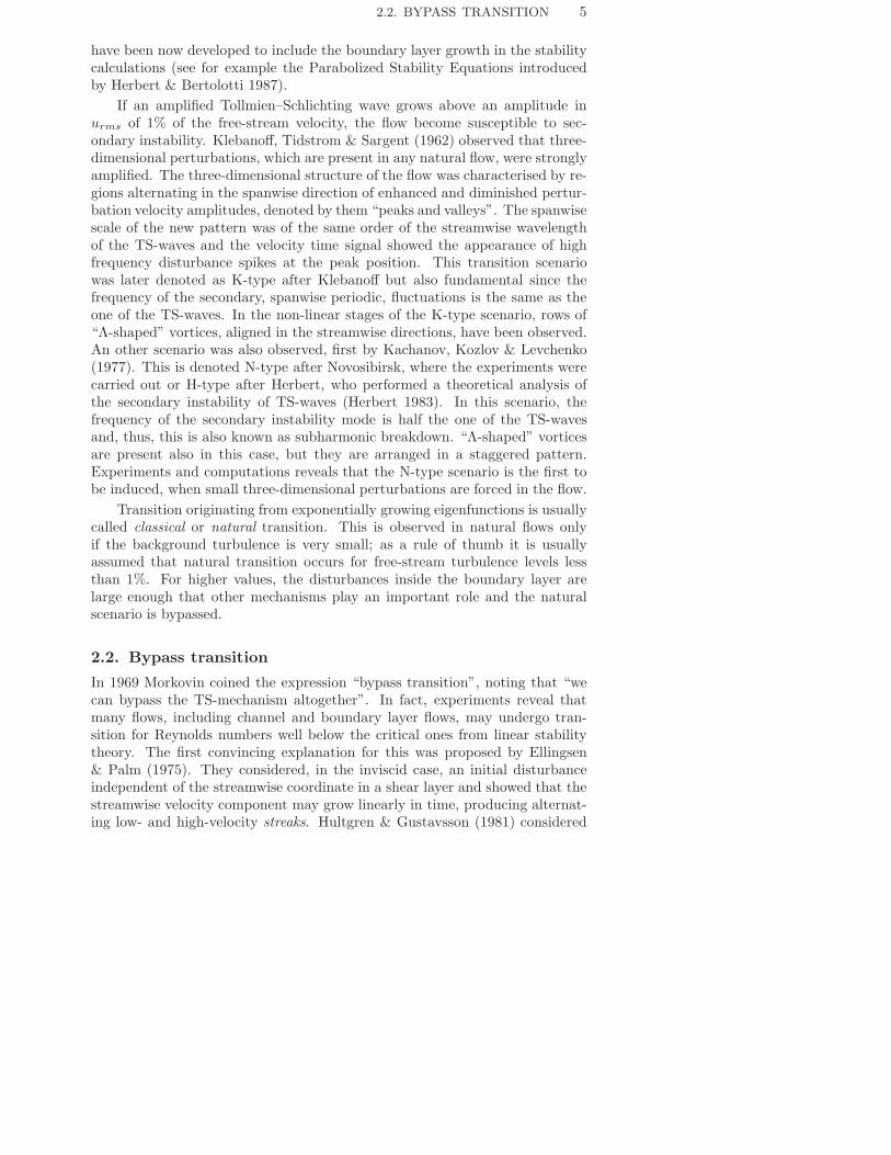
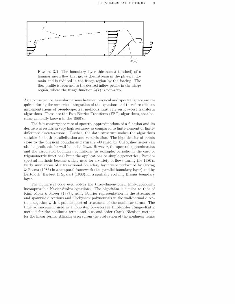
Figure 3.1. The boundary layer thickness δ (dashed) of alaminar mean flow that grows downstream in the physical do-main and is reduced in the fringe region by the forcing. Theflow profile is returned to the desired inflow profile in the fringeregion, where the fringe function λ(x) is non-zero.

As a consequence, transformations between physical and spectral space are re-quired during the numerical integration of the equations and therefore efficientimplementations of pseudo-spectral methods must rely on low-cost transformalgorithms. These are the Fast Fourier Transform (FFT) algorithms, that be-came generally known in the 1960’s.

The fast convergence rate of spectral approximations of a function and itsderivatives results in very high accuracy as compared to finite-element or finite-difference discretizations. Further, the data structure makes the algorithmssuitable for both parallelisation and vectorisation. The high density of pointsclose to the physical boundaries naturally obtained by Chebyshev series canalso be profitable for wall-bounded flows. However, the spectral approximationand the associated boundary conditions (as example, periodic in the case oftrigonometric functions) limit the applications to simple geometries. Pseudo-spectral methods became widely used for a variety of flows during the 1980’s.Early simulations of a transitional boundary layer were performed by Orszag& Patera (1983) in a temporal framework (i.e. parallel boundary layer) and byBertolotti, Herbert & Spalart (1988) for a spatially evolving Blasius boundarylayer.

The numerical code used solves the three-dimensional, time-dependent,incompressible Navier-Stokes equations. The algorithm is similar to that ofKim, Moin & Moser (1987), using Fourier representation in the streamwiseand spanwise directions and Chebyshev polynomials in the wall-normal direc-tion, together with a pseudo-spectral treatment of the nonlinear terms. Thetime advancement used is a four-step low-storage third-order Runge–Kuttamethod for the nonlinear terms and a second-order Crank–Nicolson methodfor the linear terms. Aliasing errors from the evaluation of the nonlinear terms

10 3. DIRECT NUMERICAL SIMULATIONS

are removed by the 32 -rule when the FFTs are calculated in the wall parallel

plane. In order to set the free-stream boundary condition closer to the wall,a generalisation of the boundary condition used by Malik, Zang & Hussaini(1985) is employed. It is an asymptotic condition applied in Fourier space withdifferent coefficients for each wavenumber that exactly represents a potentialflow solution decaying away from the wall.

To correctly account for the downstream boundary layer growth a spatialtechnique is necessary. This requirement is combined with the periodic bound-ary condition in the streamwise direction by the implementation of a “fringeregion”, similar to that described by Bertolotti, Herbert & Spalart (1992). Inthis region, at the downstream end of the computational box, the function λ(x)in equation (3.1) is smoothly raised from zero and the flow is forced to a desiredsolution v in the following manner,

∂u∂t

= NS(u) + λ(x)(v − u) + g, (3.1)

∇ · u = 0, (3.2)

where u is the solution vector and NS(u) the right hand side of the (unforced)momentum equations. Both g, which is a disturbance forcing, and v maydepend on the three spatial coordinates and time. The forcing vector v issmoothly changed from the laminar boundary layer profile at the beginning ofthe fringe region to the prescribed inflow velocity vector. This is normally aboundary layer profile v0, but can also contain a disturbance. This methoddamps disturbances flowing out of the physical region and smoothly trans-forms the flow to the desired inflow state, with a minimal upstream influence(see Nordstrom et al. 1999, for an investigation of the fringe region technique).Figure 3.1 illustrates the variation of the boundary layer thickness in the com-putational box for a laminar case together with a typical fringe function λ(x).

3.2. Disturbance generation

Using this numerical code, disturbances can be introduced in the laminar flowby including them in the flow field v, thereby forcing them in the fringe region;by a body force g, and by blowing and suction at the wall through non ho-mogeneous boundary conditions. The first of these three methods is the mostused in the simulations presented in the thesis. In fact, to study the instabilityand breakdown of steady, spanwise periodic streaks, the velocity fields vs andvd are added to the Blasius solution v0 to give a forcing vector of the formv = v0 + vs + vde

iωt. vs represents the steady streaks: those linear optimalcomputed by Andersson et al. (1999) are forced at the inflow in Paper 1 andthe nonlinearly saturated streaks obtained are then used as inlet conditions insome of the following studies. The time periodic disturbance vd is an insta-bility mode riding on the streak which is used to simulate the full transitionprocess of a steady streak in Paper 3.

To simulate a boundary layer under free-stream turbulence (Paper 7) amore involved methodology has been implemented. Following Jacobs & Durbin

3.2. DISTURBANCE GENERATION 11

(2001), a turbulent inflow is described as a superposition of modes of the contin-uous spectrum of the linearised Orr-Sommerfeld and Squire operators. Thesemodes have also been added to the forcing vector v and thus introduced in thefringe region. Isotropic grid turbulence can be reproduced by a sum of Fouriermodes with random amplitudes (see Rogallo 1981); however in the presence ofan inhomogeneous direction an alternative complete basis is required; in partic-ular, in the present case, the new basis functions need to accommodate the wall.A natural choice is therefore the use of the modes of the continuous spectrum.It is useful to recall, in fact, that the Orr-Sommerfeld and Squire eigenvalueproblem for a parallel flow in a semi-bounded domain is characterised by acontinuous and a discrete spectrum (Grosch & Salwen 1978). The discretemodes decay exponentially with the distance from the wall, while modes ofthe continuous spectrum are nearly sinusoidal in the free stream. As a con-sequence, a three-dimensional wave-vector κ = (α, γ, β) can be associated toeach eigenfunction of the continuous spectrum: The streamwise and spanwisewave numbers α and β are defined by the normal mode expansion in the ho-mogeneous directions of the underlying linear problem while the wall-normalwavelength is determined by the eigenvalue along the continuous spectrum. In-voking Taylor’s hypothesis, the streamwise wavenumber α can be replaced bya frequency ω = αU∞ and the expansion may be written

u =∑

AN uN (y) e(iβz+iαx−iωt),

where the real values of β and ω and the complex wavenumber α are selectedaccording to the procedure described below. Note that the desired wall-normalwavenumber γ enters through the eigenfunction shape uN (y) and it is definedby the eigenvalue α. In particular, the wave numbers pertaining to the modesused in the expansion are selected by defining in the wavenumber space (ω, γ, β)a number of spherical shells of radius |κ|. 40 points are then placed randomlybut at equal intervals on the surface of these spheres. The coordinates of thesepoints define the wave numbers of the modes used in the expansion above. Thecomplex coefficients AN provide random phase but a given amplitude. Theamplitude |AN | is in fact the same for all modes on each shell and reproduces thefollowing analytical expression for a typical energy spectrum of homogeneousisotropic turbulence

E(κ) =23

a (κL)4

(b+ (κL)2)17/6LTu. (3.3)

In the expression above, Tu is the turbulence intensity, L a characteristic inte-gral length scale and a, b two normalisation constants. The methodology brieflyintroduced here is able to satisfactorily reproduce a boundary layer subject tofree-stream turbulence as documented in Paper 7.

CHAPTER 4

Instability and breakdown of steady optimal streaks

4.1. Steady saturated streaks

The two linear disturbance-growth mechanisms usually encountered in flat-plate boundary layers have been introduced in chapter 2. These are the ex-ponential growth of Tollmien-Schlichting waves and the transient growth ofstreamwise elongated streaks. If the amplification of either of the two is largeenough, the disturbances eventually reach an amplitude where nonlinear ef-fects become relevant. These primary perturbations saturate and take the flowinto a new more complicated steady or quasi-steady laminar state. The lin-ear stability of this new flow configuration is the object of secondary stabilityinvestigations.

The analysis performed here concerns the linear secondary stability of thestreaks resulting from the nonlinear evolution of the spatial optimal pertur-bation in a Blasius boundary layer. The investigation is motivated by theneed to understand in a simpler configuration the physics of bypass transi-tion in boundary layers with high levels of free-stream turbulence, where lowfrequency streaks are the type of perturbations induced inside the boundarylayer. The base flows under consideration are computed by solving the fullNavier-Stokes equations (see Paper 1). In particular, the complete velocityfield representing the initial evolution of the steady, spanwise periodic, linearoptimal perturbations calculated by Andersson et al. (1999), is forced in thefringe region as described in the previous chapter. The downstream nonlineardevelopment of the streaks is monitored for different upstream amplitudes ofthe input disturbance. To quantify the size of this primary disturbance at eachstreamwise position, an amplitude A is defined as

A(X) =12

[maxy,z

(U(X, y, z) − UB(X, y)

)− min

y,z

(U(X, y, z)− UB(X, y)

)],

where UB(x, y) is the Blasius profile and U(X, y, z) is the total streamwisevelocity in the presence of streaks and they are made non dimensional withrespect to the free-stream velocity U∞.

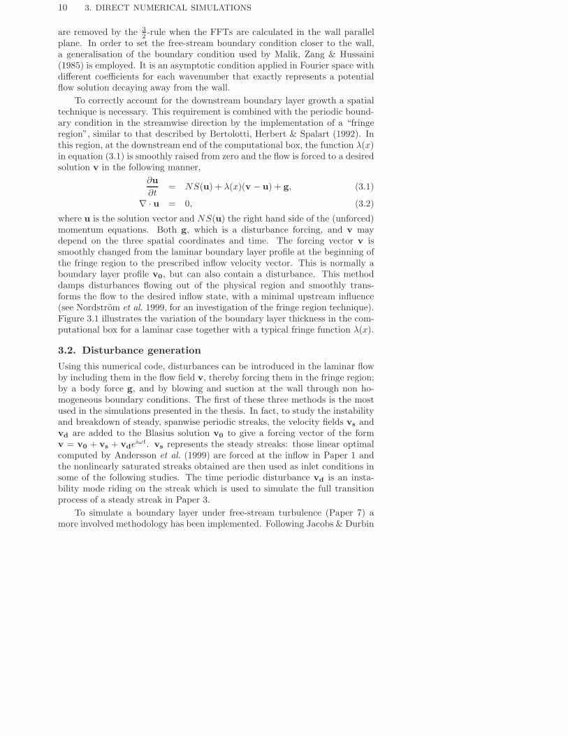
The downstream amplitude development is displayed in figure 4.1(a) forthe set of upstream amplitudes considered. The abscissa X in the figure in-dicates the distance from the leading edge and it is divided by the referencelength L, where L = 1 is the station at which the linear growth of the upstream

12

4.1. STEADY SATURATED STREAKS 13

0.5 1 1.5 2 2.5 30.05

0.15

0.25

0.35

0.45

−2 −1 0 1 20

1

2

3

4

5

6

A

(a) (b)

y

zX

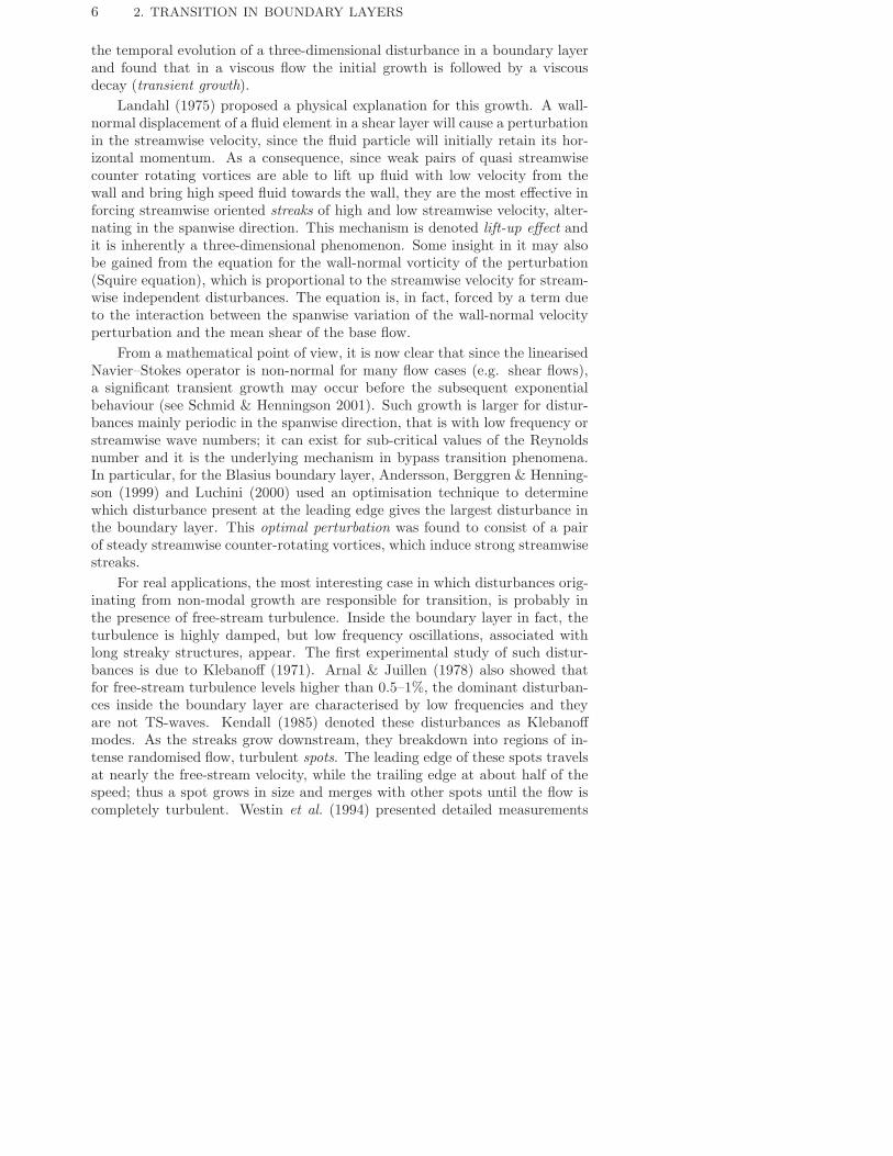
Figure 4.1. (a) Downstream development of the streak am-plitude A versus streamwise coordinate X for different up-stream amplitudes A0. (b) Streamwise velocity contour plot ofthe nonlinear base flow in a (y, z) cross-stream plane at X = 2,A = 0.36. The coordinates have been made non-dimensionalsing the local Blasius length scale δ. Maximum contour level0.98, contour spacing 0.1.

streamwise vortices has been optimised (see Andersson et al. 1999). The span-wise wavenumber β = 0.45 is the optimal one and it is scaled with respectto the local Blasius length δ =

√xν/U∞ at position x = L. In figure 4.1(b),

a typical nonlinearly saturated streak is illustrated by its streamwise velocitycontour plot in the cross-stream (y, z) plane. Regions of strong spanwise shearare formed on the sides of the low-speed region, which is also displaced furtheraway from the wall during the saturation process.

It is worth introducing a scaling property of the considered nonlinearstreaks which will be used to extend the validity of the results obtained, toa wide range of Reynolds numbers and spanwise wave numbers. In fact, itis shown in Paper 1 that a streak family U(x, y, z), defined by the upstreamamplitude A0 and by the spanwise wavenumber β0 at the inlet X0, obeys theboundary layer equations and it is therefore independent of the Reynolds num-ber if scaled by the boundary layer scalings. This results in a scaling propertythat couples the streamwise and spanwise scales, implying that the same so-lution is valid for every combination of x = x∗/L and β = β∗δ such that theproduct xβ2 stays constant (the star denotes dimensional quantities). Alter-natively, one could consider the product between the local Reynolds numberbased on the distance from the leading edge Rex = U∞x∗/ν and the wavenum-ber β = β∗ν/U∞ and keep Rexβ

2 = const. In other words, it is possible tofreely choose the local Reynolds number pertaining to a given streak profileU(y, z). This amounts to moving along the plate and varying the spanwisewavenumber β0 so that the local spanwise wavenumber β0δ/δ0, where δ0 indi-cates the local Blasius thickness at the upstream positionX0, remains constant.Note also that in the non dimensional form of the boundary layer equations

14 4. INSTABILITY AND BREAKDOWN OF STEADY STREAKS

the cross-stream velocities v and w are multiplied by the Reynolds numberRe =

√Rex. As a consequence, the amplitude of the initial vortex needed to

produce a fixed amplitude of the streak along the curve Rexβ2 = const de-

creases in a manner inversely proportional to the square root of Rex. Usingthe coupling between the streamwise and spanwise scales, this corresponds tosay that the amplitude of the initial vortex is proportional to the spanwisewavenumber β.

4.2. Streak instability

If the amplitude of the streak grows to a sufficiently high value, instabilitiescan develop which may provoke early breakdown and transition to turbulencedespite the predicted modal decay of the primary disturbance. A possiblesecondary instability is caused by inflectional profiles of the base flow velocity,a mechanism which does not rely on the presence of viscosity.

In flows over concave walls or in rotating channels, the primary exponentialinstability results in streamwise vortices, which, in turn, create streaks. It istherefore not surprising that the first studies on the secondary instability ofstreaky structures refer to these types of flows and it can be expected that thesecondary instability mechanisms of the flat-plate boundary-layer streaks con-sidered here will show similarities with the instabilities observed in the flowsmentioned above (see Schmid & Henningson 2001 among others). The exper-iments of Swearingen & Blackwelder (1987) were the first to document theemergence of streaks with inflectional profiles due to the formation of stream-wise vortices (called Gortler vortices) in the boundary layer over a concavewall. This investigation demonstrated that time-dependent fluctuations ap-pear in the flow either in a spanwise symmetric (varicose) or antisymmetric(sinuous) pattern with respect to the underlying streak. The varicose pertur-bations are more closely related with the wall-normal inflection points whilethe sinuous oscillations are related with the spanwise inflectional profile andthey were found to be the fastest growing. These findings were successivelyconfirmed by theoretical analysis of the instability of Gortler vortices, bothassuming inviscid flow and including the effect of viscosity (e.g. Park & Huerre1995; Bottaro & Klingmann 1996). The instability of streaks arising from thetransient growth of streamwise vortices in channel flows has been studied the-oretically by Waleffe (1995, 1997) and Reddy et al. (1998) and experimentallyby Elofsson, Kawakami & Alfredsson (1999). These studies confirmed that theinstability is of inflectional type and that the dominating instability appearsas spanwise (sinuous) oscillations of the streaks.

The secondary instability of the steady, spanwise periodic streaks intro-duced in the previous section is studied under two basic assumptions. Sincethe streaks satisfy the boundary layer approximation, the downstream variationof the streamwise velocity is slow and the wall-normal and spanwise velocitiesare very small, of the order O(1/Re1/2

x ), as compared to the streamwise com-ponent. Therefore the basic flow will consist only of the streamwise velocity

4.2. STREAK INSTABILITY 15

U . Further, the secondary instability is observed in flow visualisations to varyrapidly in the streamwise direction. Hence, we will assume a parallel mean flowU(y, z), dependent only on the cross-stream coordinates. This basic parallelflow is extracted at different streamwise stations X from the spatial numericalsimulations presented in figure 4.1.

The equations governing the linear evolution of a perturbation velocityu(x, y, z, t) = (u, v, w), of corresponding pressure p, on the streak profile U(y, z)are obtained by substituting U + u into the Navier-Stokes equations and ne-glecting the quadratic terms in the perturbation. This yields

ut + Uux + Uyv + Uzw = −px +1Re

∆u, (4.1)

vt + Uvx = −py +1Re

∆v, (4.2)

wt + Uwx = −pz +1Re

∆w, (4.3)

ux + vy + wz = 0. (4.4)

Following a procedure similar to that used in the derivation of the Orr-Sommerfeldand Squire system, the above equations can be reduced to two equations interms of the normal velocity v and the normal vorticity η = vz − wx

∆vt + U∆vx + Uzzvx + 2Uzvxz − Uyyvx − 2Uzwxy − 2Uyzwx = 1Re∆∆v,

ηt + Uηx − Uzvy + Uyzv + Uyvz + Uzzw = 1Re∆η.

(4.5)In the above, the spanwise velocity w can be eliminated by using the identity

wxx + wzz = −ηx − vyz .

Since the flow is assumed parallel, solution can be sought in the form ofstreamwise waves. Further, due to the spanwise periodicity of the flow, Floquettheory can be applied (e.g. Nayfeh & Mook 1979). As a consequence, for anyflow quantity q, the instability modes of the basic flow U of spanwise wavelengthλz = 2π/β may be expressed in the form

q(x, y, z, t) = q(y, z) ei [α x+θ z−ωt], (4.6)

where q is spanwise periodic and it has the same periodicity λz of the basicflow. α, the streamwise wavenumber, and ω, the circular frequency, can assumecomplex values; θ is a real detuning parameter or Floquet exponent. Due tothe spanwise symmetry of the basic streak profile U(y, z) (see figure 4.1b),the modes can be divided into separate classes according to their odd or evensymmetry. Further, it is sufficient to study values of the parameter θ betweenzero and π/λz , with θ = 0 corresponding to a fundamental instability mode ofspanwise wavelength λz and θ = π/λz corresponding to a subharmonic mode ofwavelength twice that of the underlying streak. Symmetric and antisymmetricmodes are called varicose and sinuous respectively, with reference to the visualappearance of the motion of the low-speed streak.


x

z

�

�

Fundamental sinuous Subharmonic sinuous

Fundamental varicose Subharmonic varicose

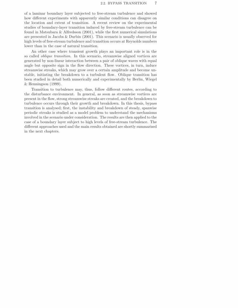
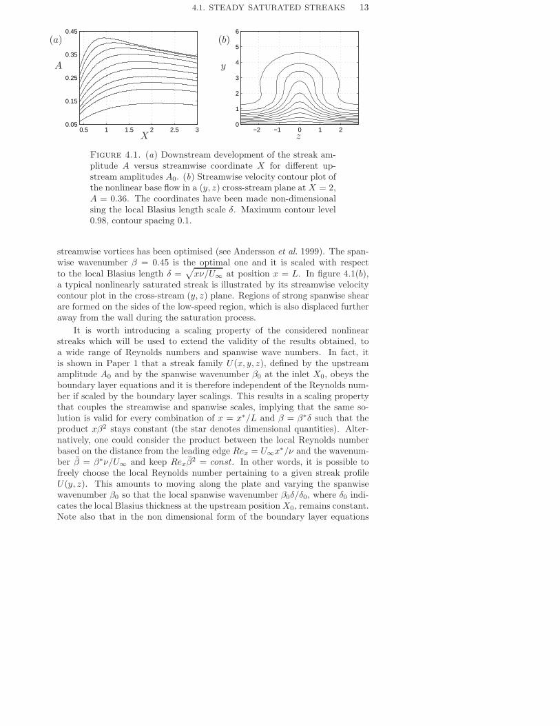
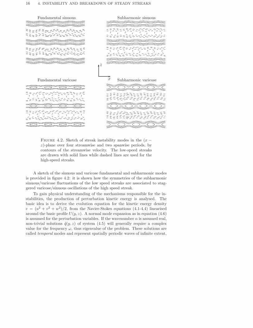
Figure 4.2. Sketch of streak instability modes in the (x −z)-plane over four streamwise and two spanwise periods, bycontours of the streamwise velocity. The low-speed streaksare drawn with solid lines while dashed lines are used for thehigh-speed streaks.

A sketch of the sinuous and varicose fundamental and subharmonic modesis provided in figure 4.2: it is shown how the symmetries of the subharmonicsinuous/varicose fluctuations of the low speed streaks are associated to stag-gered varicose/sinuous oscillations of the high speed streak.

To gain physical understanding of the mechanisms responsible for the in-stabilities, the production of perturbation kinetic energy is analysed. Thebasic idea is to derive the evolution equation for the kinetic energy densitye = (u2 + v2 + w2)/2, from the Navier-Stokes equations (4.1-4.4) linearisedaround the basic profile U(y, z). A normal mode expansion as in equation (4.6)is assumed for the perturbation variables. If the wavenumber α is assumed real,non-trivial solutions q(y, z) of system (4.5) will generally require a complexvalue for the frequency ω, thus eigenvalue of the problem. These solutions arecalled temporal modes and represent spatially periodic waves of infinite extent,


travelling with phase velocity cr = wr/α and being damped or amplified attemporal growth rate ωi (the suffix r and i indicate the real and imaginarypart respectively). This type of modes is considered in the analysis of the per-turbation kinetic energy production. Upon integration over a wavelength of thesecondary mode in the streamwise and spanwise directions and from the wallto infinity in the wall-normal direction, the divergence terms in the evolutionequation give a zero global contribution to the energy balance and one is leftwith

∂E

∂t= Ty + Tz − D, (4.7)

where

E =1λz

∫ λz

0

∫ ∞

0

e dy dz , D =1λz

∫ λz

0

∫ ∞

0

d dy dz, (4.8)

Ty =1λz

∫ λz

0

∫ ∞

0

τuv∂U

∂ydy dz , Tz =

1λz

∫ λz

0

∫ ∞

0

τuw∂U

∂zdy dz, (4.9)

and

e = (uu∗ + vv∗ + ww∗) , d = 2(ξξ∗ + ηη∗ + ζ ζ∗

)/Re,

τuv = − (uv∗ + u∗v) , τuw = − (uw∗ + u∗w) .

The quantity E is the total perturbation kinetic energy and D is the vis-cous dissipation term given by the square of the perturbation vorticity vector(ξ, η, ζ). Ty and Tz are the perturbation kinetic energy production terms asso-ciated with the work of the Reynolds stresses τuv and τuw against, respectively,the wall-normal shear ∂U/∂y and spanwise shear ∂U/∂z of the basic flow. Thefollowing identity is immediately derived from equation (4.7) by noting that thequadratic quantities (E, D, Ty, Tz) have an exponential time behaviour e2ωit:

ωi =Ty

2E+Tz

2E− D

2E. (4.10)

In order to evaluate the different terms entering equation (4.10) one has tosolve the system (4.5) for the eigenmode and eigenvalue corresponding to theselected velocity profile U(y, z), Reynolds number and streamwise wavenumberα. In the absence of errors in the computation, the left-hand side, comingfrom the eigenvalue computation, and the right-hand side derived from thecorresponding mode shape, should match. Equation (4.10) provides an insightinto the instability mechanisms by separating the three terms which contributeto the temporal growth rate ωi. An instability is seen to appear when thework of the Reynolds stresses against the basic shears is positive and able toovercome viscous dissipation.


4.2.1. Viscous instabilities in low-amplitude streaks

According to Rayleigh’s criterion, velocity profiles without inflection points,typical of wall-bounded shear flows such as the Blasius boundary layer of inter-est here, are linearly stable in the inviscid approximation. However, it is demon-strated that viscous effects may, paradoxically, be destabilising for a range offinite Reynolds number thus leading to the growth of the Tollmien-Schlichtingwaves. Inviscid instabilities develop on a convective time scale τi ≈ L/v, withL and v characteristic length and velocity. For flows destabilised by viscosityinstead, the growth rates are smaller and the perturbation evolves on a diffusivetime scale τv ≈ L2/ν.

As discussed earlier, small amounts of streamwise vorticity in a laminarboundary layer are very effective in moving low-momentum particles away fromthe wall and high-momentum particles toward the wall, thus forming elongatedspanwise modulations of the streamwise velocity. Since streamwise streaks canbe expected to arise whenever a boundary layer is subject to weak perturbationswith streamwise vorticity, it is interesting to study the behaviour of the viscousinstability in a streaky boundary layer. This analysis is the first step in thestudy of the effect of streamwise vortices and streaks on the transition in theBlasius boundary layer and it can be considered more relevant in the case oflow-amplitude stable streaks.

Previous experimental work on the subject have given somewhat surprisingresults. Kachanov & Tararykin (1987) generated streamwise steady streaks byblowing and suction at the wall and used a vibrating ribbon to generate TS-waves. They found three-dimensional waves, modulated by the underlyingstreaks, having essentially the same phase speed as the TS-waves developingin an undisturbed Blasius boundary layer, but with lower growth rates. Boikoet al. (1994) also forced TS-waves with a vibrating ribbon but in a boundarylayer subject to free-stream turbulence, therefore with randomly appearinglow-frequency streaks. They also found waves less amplified than in a two-dimensional Blasius flow.

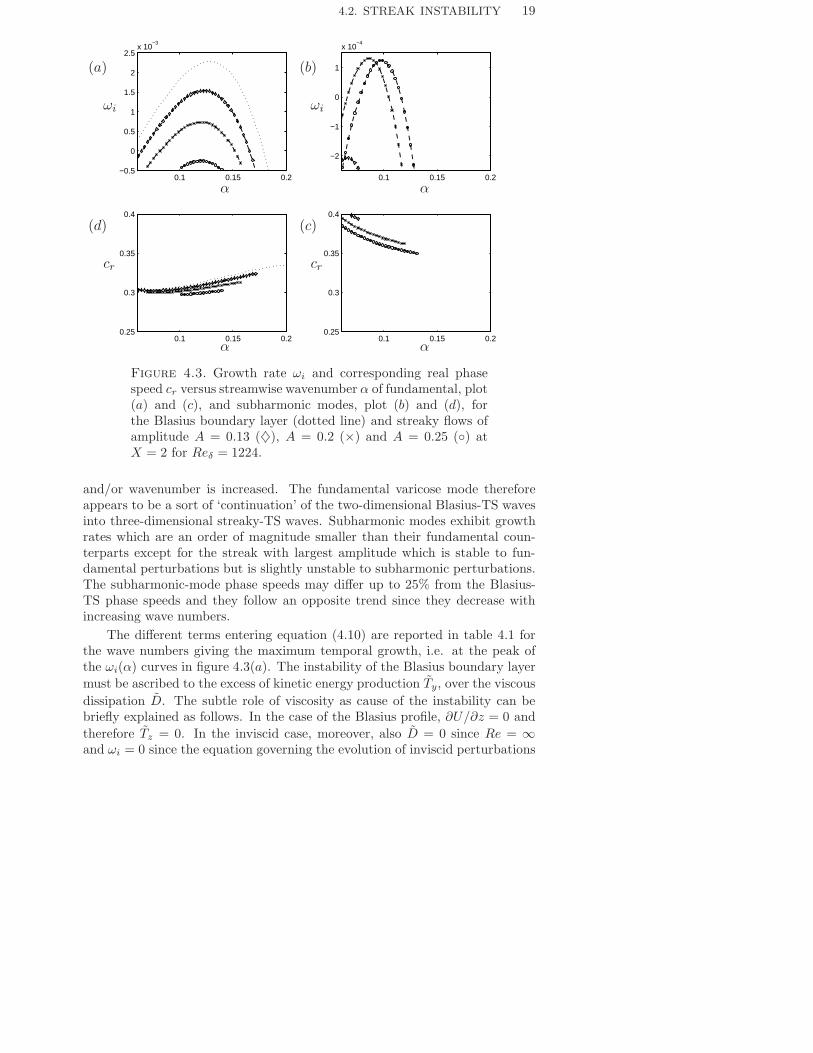
Before considering the different energy production terms in equation (4.10),the viscous temporal stability of the steady optimal streaks presented in fig-ure 4.1(a) is studied. The eigenvalues having largest imaginary part ωi arecomputed over a range of wave numbers α for the Blasius boundary layer andthree streak profiles extracted at position X = 2. The local Reynolds numberis selected to be Re = 1224. Note that all the streaks under consideration arestable in the inviscid approximation, as shown in the next section. The tem-poral growth rate curves ωi(α) and the corresponding phase speeds cr = ωr/αof varicose perturbations of respectively fundamental and subharmonic typeare displayed in figure 4.3. Sinuous perturbations resulted stable. Increasingthe amplitude of the streak reduces the growth rates of fundamental modesup to their complete stabilisation for the largest amplitude considered. Thephase speeds of the fundamental modes are roughly unchanged with respectto the Blasius-TS waves; they are only are slightly reduced as the amplitude


0.1 0.15 0.2−0.5

0

0.5

1

1.5

2

2.5x 10

−3

0.1 0.15 0.20.25

0.3

0.35

0.4

0.1 0.15 0.2

−2

−1

0

1

x 10−4

0.1 0.15 0.20.25

0.3

0.35

0.4

(a)

ωi

(b)

ωi

(c)

cr cr

(d)

α α

α α

Figure 4.3. Growth rate ωi and corresponding real phasespeed cr versus streamwise wavenumber α of fundamental, plot(a) and (c), and subharmonic modes, plot (b) and (d), forthe Blasius boundary layer (dotted line) and streaky flows ofamplitude A = 0.13 (♦), A = 0.2 (×) and A = 0.25 (◦) atX = 2 for Reδ = 1224.

and/or wavenumber is increased. The fundamental varicose mode thereforeappears to be a sort of ‘continuation’ of the two-dimensional Blasius-TS wavesinto three-dimensional streaky-TS waves. Subharmonic modes exhibit growthrates which are an order of magnitude smaller than their fundamental coun-terparts except for the streak with largest amplitude which is stable to fun-damental perturbations but is slightly unstable to subharmonic perturbations.The subharmonic-mode phase speeds may differ up to 25% from the Blasius-TS phase speeds and they follow an opposite trend since they decrease withincreasing wave numbers.

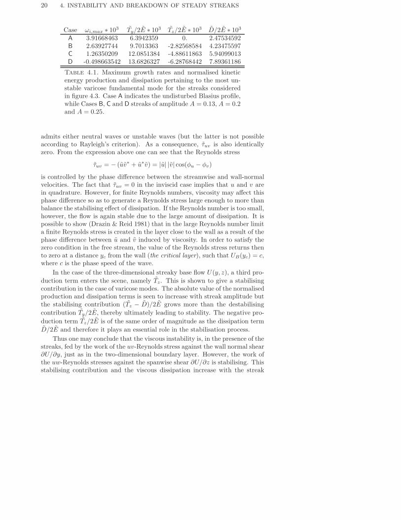
The different terms entering equation (4.10) are reported in table 4.1 forthe wave numbers giving the maximum temporal growth, i.e. at the peak ofthe ωi(α) curves in figure 4.3(a). The instability of the Blasius boundary layermust be ascribed to the excess of kinetic energy production Ty, over the viscousdissipation D. The subtle role of viscosity as cause of the instability can bebriefly explained as follows. In the case of the Blasius profile, ∂U/∂z = 0 andtherefore Tz = 0. In the inviscid case, moreover, also D = 0 since Re = ∞and ωi = 0 since the equation governing the evolution of inviscid perturbations


Case ωi,max ∗ 103 Ty/2E ∗ 103 Tz/2E ∗ 103 D/2E ∗ 103

A 3.91668463 6.3942359 0. 2.47534592B 2.63927744 9.7013363 -2.82568584 4.23475597C 1.26350209 12.0851384 -4.88611863 5.94099013D -0.498663542 13.6826327 -6.28768442 7.89361186

Table 4.1. Maximum growth rates and normalised kineticenergy production and dissipation pertaining to the most un-stable varicose fundamental mode for the streaks consideredin figure 4.3. Case A indicates the undisturbed Blasius profile,while Cases B, C and D streaks of amplitude A = 0.13, A = 0.2and A = 0.25.

admits either neutral waves or unstable waves (but the latter is not possibleaccording to Rayleigh’s criterion). As a consequence, τuv is also identicallyzero. From the expression above one can see that the Reynolds stress

τuv = − (uv∗ + u∗v) = |u| |v| cos(φu − φv)

is controlled by the phase difference between the streamwise and wall-normalvelocities. The fact that τuv = 0 in the inviscid case implies that u and v arein quadrature. However, for finite Reynolds numbers, viscosity may affect thisphase difference so as to generate a Reynolds stress large enough to more thanbalance the stabilising effect of dissipation. If the Reynolds number is too small,however, the flow is again stable due to the large amount of dissipation. It ispossible to show (Drazin & Reid 1981) that in the large Reynolds number limita finite Reynolds stress is created in the layer close to the wall as a result of thephase difference between u and v induced by viscosity. In order to satisfy thezero condition in the free stream, the value of the Reynolds stress returns thento zero at a distance yc from the wall (the critical layer), such that UB(yc) = c,where c is the phase speed of the wave.

In the case of the three-dimensional streaky base flow U(y, z), a third pro-duction term enters the scene, namely Tz. This is shown to give a stabilisingcontribution in the case of varicose modes. The absolute value of the normalisedproduction and dissipation terms is seen to increase with streak amplitude butthe stabilising contribution (Tz − D)/2E grows more than the destabilisingcontribution Ty/2E, thereby ultimately leading to stability. The negative pro-duction term Tz/2E is of the same order of magnitude as the dissipation termD/2E and therefore it plays an essential role in the stabilisation process.

Thus one may conclude that the viscous instability is, in the presence of thestreaks, fed by the work of the uv-Reynolds stress against the wall normal shear∂U/∂y, just as in the two-dimensional boundary layer. However, the work ofthe uw-Reynolds stresses against the spanwise shear ∂U/∂z is stabilising. Thisstabilising contribution and the viscous dissipation increase with the streak


amplitude, thereby reducing the growth rate and eventually leading to stability.These results enable to envision a possible control strategy for applications inboundary-layer transition delay in low-noise environment where the classicaltransition scenario is the most likely to occur. Further investigation is neededon possible streak-generation schemes and on the computation of total spatialgrowth-rate reductions in the presence of streaks.

4.2.2. Inviscid instability

As discussed earlier, high-amplitude streak develop inflectional profiles whichcan lead to strong inviscid secondary instabilities. Therefore, the marginalcondition for streak instability is investigated here under the assumption ofinviscid flow. If viscosity is neglected it is possible to find an uncoupled equationfor the perturbation pressure (Henningson 1987; Hall & Horseman 1991)

(∂

∂t+ U

∂

∂x)∆p− 2Uypxy − 2Uzpxz = 0. (4.11)

This equation governs the linear stability of a parallel streak. Such basic flowis said to be stable in the inviscid approximation, if all possible perturbationssuperposed on the streak are damped. On the contrary, if some perturbationsgrow in amplitude the flow is said to be unstable. In the control parame-ter space, two domains corresponding to either stability or instability may beidentified. These are separated by the so called neutral surface.

The inviscid instability is analysed in the temporal framework so that acomplex value for the frequency ω is obtained as eigenvalue of the system (4.11).The flow is thus unstable if it is possible to find a value of α for which ωi > 0.Further it is possible to show that when all temporal modes are damped, theflow is linearly stable (e.g. Huerre & Rossi 1998). Thus, a temporal analysiscompletely determines the stability or instability of a given flow.

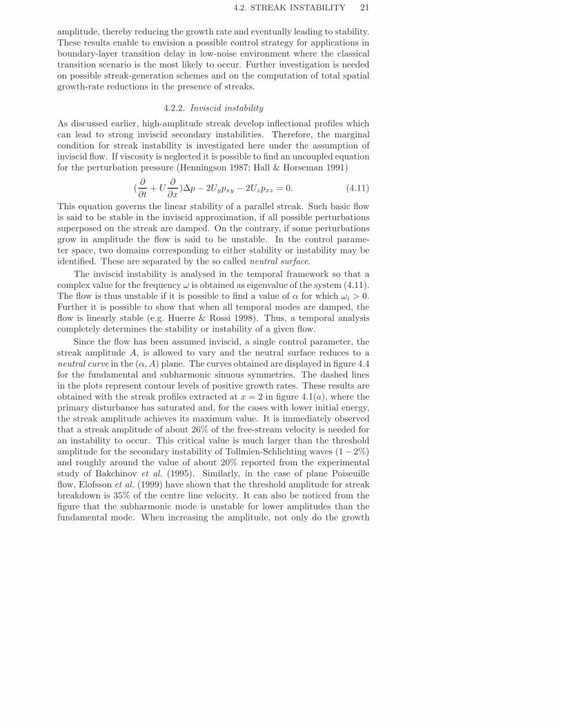
Since the flow has been assumed inviscid, a single control parameter, thestreak amplitude A, is allowed to vary and the neutral surface reduces to aneutral curve in the (α,A) plane. The curves obtained are displayed in figure 4.4for the fundamental and subharmonic sinuous symmetries. The dashed linesin the plots represent contour levels of positive growth rates. These results areobtained with the streak profiles extracted at x = 2 in figure 4.1(a), where theprimary disturbance has saturated and, for the cases with lower initial energy,the streak amplitude achieves its maximum value. It is immediately observedthat a streak amplitude of about 26% of the free-stream velocity is needed foran instability to occur. This critical value is much larger than the thresholdamplitude for the secondary instability of Tollmien-Schlichting waves (1− 2%)and roughly around the value of about 20% reported from the experimentalstudy of Bakchinov et al. (1995). Similarly, in the case of plane Poiseuilleflow, Elofsson et al. (1999) have shown that the threshold amplitude for streakbreakdown is 35% of the centre line velocity. It can also be noticed from thefigure that the subharmonic mode is unstable for lower amplitudes than thefundamental mode. When increasing the amplitude, not only do the growth


0.27 0.29 0.31 0.33 0.35 0.37

0.2

0.4

0.6

0.8

0.25 0.27 0.29 0.31 0.33 0.35 0.37

0.2

0.4

0.6

0.8

α

(a) (b)

α

AA

Figure 4.4. Neutral curves for streak instability in the (α,A)plane (solid line). The dashed lines represent contour levels ofpositive growth rates ωi = 0.008 and ωi = 0.016. The datahave been made non-dimensional using the local Blasius lengthscale δ.

rates increase but their maxima are also shifted towards larger values of thewavenumber α. For values of A larger than 0.3 the fundamental symmetry hasslightly larger growth rates. It is also found that in the case of the sinuousinstability, the production of kinetic energy of the perturbation is entirely dueto the work of the Reynolds stress τuw against the spanwise shear of the streak.The contribution from the term Ty, related to the wall-normal shear of the basicflow, is negative and about one order of magnitude smaller than its counterpartTz.

No results are presented here on the varicose instabilities. In fact, thevaricose modes result unstable only for amplitudes larger than A = 0.37, withgrowth rates smaller than one fifth of the corresponding sinuous growth rates.From the results presented, it seems more likely that the transition of theconsidered steady optimal streaks is triggered by a sinuous instability, either offundamental or subharmonic type. The common feature of the two scenariosis the spanwise oscillation of the low-speed streak.

4.2.3. Spatio-temporal behaviour

The boundary layer flow is an open flow, i.e. the fluid particles are not recycledwithin the physical domain of interest but leave it in a finite time (see Huerre& Monkewitz 1990). Linearly unstable open flows can be classified accordingto the evolution of amplified perturbations in space and time into two distinctclasses. To introduce this distinction, we consider the response of the systemto an impulse in space and time δ(t)δ(x). The flow is initially perturbed att = 0 and x = 0 and left free to evolve. The solution to this problem representsthe Green function G(x, t) of the particular linear system under considerationsand contains the information concerning the evolution of any disturbances. In


fact, the response to any forcing functions may be obtained by convolution ofsuch forcing with the Green function.

In linearly unstable flows, two distinct asymptotic behaviours of the im-pulse response can be observed. The flow is said to be linearly convectivelyunstable if the amplified perturbations are convected away, downstream orupstream of the source, so that the perturbation ultimately decreases at anylocation and the flow returns to its basic state as t → ∞. Conversely, a flowis said to be linearly absolutely unstable if the disturbance generated by theimpulse spreads both upstream and downstream of the source and graduallycontaminates the entire medium.

Formally, a given flow is convectively unstable if

limt→∞G(x, t) = 0, along the ray x/t = 0

and absolutely unstable if

limt→∞G(x, t) = ∞, along the ray x/t = 0.

In the case of parallel flows, that are invariant under Galileian transforma-tions, this distinction seems to be related to the selected frame of reference:a simple change of reference frame may transform an absolutely unstable flowinto a convectively unstable. However, in flows forced at a specific streamwisestation x the Galileian invariance is broken and a ’laboratory frame’ can beunambiguously defined. In these cases, the distinction between convective andabsolute instability becomes of interest. Convectively unstable flows essentiallybehave as noise amplifiers: they are very sensitive to external perturbations.The characteristics of the latter determine, in fact, the type of waves amplify-ing in the flow. Absolutely unstable flows, on the contrary, display an intrinsicdynamics. They behave as hydrodynamic oscillators. The features of the per-turbations amplifying in the flow are determined by the control parameters anddo not depend on the external noise. The flow beats at a well-defined frequencyindependently on the frequency at which it is forced (see Huerre & Rossi 1998).

From the definitions above, it follows that the spatio-temporal analysis ofa linearly unstable flow aims at computing the asymptotic temporal growthrates σ attained along rays x/t = v, that is the temporal growth rate perceivedby an observer moving at velocity v. This is equivalent to the study in Fourier-Laplace space of modes of real group velocity v, as reviewed, for instance, inHuerre (2000). This analysis shows that the impulse response takes the form ofa wave packet, the long time behaviour along each spatio-temporal ray being(Bers 1983)

q(x, t) ∝ t−1/2 ei[α∗(v)x−ω∗(v)t], t→ ∞where α∗ and ω∗ represent the complex wavenumber and frequency observedmoving at the velocity v. The temporal growth rate σ is defined by the real partof the exponential σ = ω∗

i − v α∗i . In unstable flows, σ > 0 for some values of v

and the curve σ(v) completely defines the growth of the wave packet generatedby the impulse. The wave packet extent is determined by the rays along which


0.6 0.65 0.7 0.75 0.8 0.85 0.9 0.95 1

0

0.005

0.01

0.015

0.02

0.025

σ

v

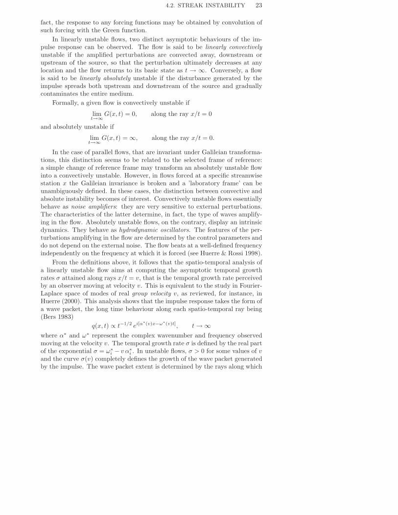
Figure 4.5. Temporal growth rate versus ray velocity x/t =v for different increasing saturated streak amplitudes A =0.28, 0.31, 0.34, 0.36, 0.38 at X = 2 computed for Re = 610.The solid line corresponds to the base flow at A = 0.36 de-picted in figure 4.1 (b). The other curves correspond to scan-ning the vertical lineX = 2 of unstable streaks in figure 4.1 (a).

neutral waves are observed, i.e. σ(v) = 0. These velocities are denoted v−,the trailing edge velocity of the wave packet, and v+ > v−, the leading edgevelocity of the wave packet. If v− > 0, the wave packet is advected downstreamand the base flow is convectively unstable. Conversely, if v− < 0, the trailingedge moves upstream and the flow is absolutely unstable.

The study of the spatio-temporal instability of the steady saturated streaksintroduced above, is presented in Paper 2. The analysis is performed in physicalspace and the instability characteristics are retrieved from the direct numericalsimulations of the response of the flow to a localised disturbance. Note that,as a consequence of the numerical code used, the spatio-temporal instability isstudied without the assumption of inviscid flow. As in the temporal stabilityanalysis discussed in the previous section, the basic flow consists only of thesteamwise velocity U(y, z) and it is assumed parallel. Since such a basic flow issolution of the Euler equations, a body force −Re−1∆U(y, z) is implementedinto the Navier-Stokes solver to compensate for diffusion and keep the flowsteady and parallel. The procedure used to evaluate the temporal growth ratesσ(v) from the evolution of the wave packet riding on the streaks is described indetail in Paper 2 and references therein. In particular, the analysis performedhere extends to the case of a three-dimensional periodic unidirectional flow thetechnique developed by Delbende, Chomaz & Huerre (1998) and Delbende &Chomaz (1998). The temporal growth rate curve of the fundamental sinuousmode versus group velocity is displayed in figure 4.5 for the unstable streakamplitudes at position X = 2 in figure 4.1(a). This diagram represents the


spatio-temporal analogue of the inviscid temporal growth rates reported infigure 4.4(a). It can be seen in figure 4.5 that the trailing edge velocity v−

is always positive and therefore it may be concluded that the instability isconvective. The growth rates ad the spreading rates ∆v = v+ − v− of the wavepacket increase with the streak amplitude and the maximum growth σ occursapproximately at the group velocity v = 0.8 for all amplitudes.

It is interesting to note that the secondary streak instability is travellingat velocities higher than those of the Tollmien-Schlichting waves in the undis-turbed Blasius boundary layer. In the latter case, in fact, the leading and trail-ing edge velocities of the wave packet are respectively v+ = 0.5 and v− = 0.36at Re = 580 (see Gaster 1975; Gaster & Grant 1975), while sinuous instabilitywaves have a trailing edge velocity of about 70% of the free-stream velocity.This difference is due to the fact that the two instabilities are driven by dis-tinct physical mechanisms. The Tollmien-Schlichting instability is viscous innature and its production is located in a low-velocity region close to the wall.The streak instability, instead, is inviscid in character and it is induced by thespanwise shear of the basic flow. It can be seen in figure 4.1(b) that the regionsof largest spanwise shear are located further up in the boundary layer wherethe local streamwise velocities are large. Thus, the instability is produced inhigh-velocity regions and this can explain the values of the group velocitiespertaining to the sinuous instability modes.

The sinuous streak instability is induced by the mean spanwise shear onthe sides of the low-velocity region as in two-dimensional wakes past a bluffbody. This similarity has been further confirmed by comparing the abso-lute/convective instability properties of the streak under consideration withthe family of wake profiles introduced by Monkewitz (1988). It is shown inPaper 2 that the streak profile U(y, z) may be approximately modelled by atwo-dimensional wake profile U(z), which is independent of the wall-normalcoordinate, provided one selects the plane parallel to the wall corresponding tothe maximum production of kinetic energy of the instability modes. As saidbefore, this roughly correspond to the location of maximum spanwise shear.

The convective nature of the secondary streak instability implies that theby-pass transition scenario considered here is noise-driven, i.e. the streaks be-have as noise amplifiers in terms of the classification introduced above. As aconsequence, transition prediction criteria cannot be only related to the con-trol parameters but they need to depend on the level of external noise. From atheoretical point of view, the convective nature of the instability implies thata spatial instability analysis of the flow has a physical significance. The spatialanalysis denotes the study of unstable modes of real frequency ω and complexwavenumber α. These represent time-periodic waves of amplitude amplifiedexponentially in the streamwise direction but constant in time at a fixed loca-tion. The study of the nonlinear stages following the spatial amplification ofthe fundamental sinuous instability mode are presented in the next section.


520 540 560 580 600 620 640 660 680 700 720

10−10

10−8

10−6

10−4

10−2

100

(0,β)

(1,β)

(2,β)

E

Re

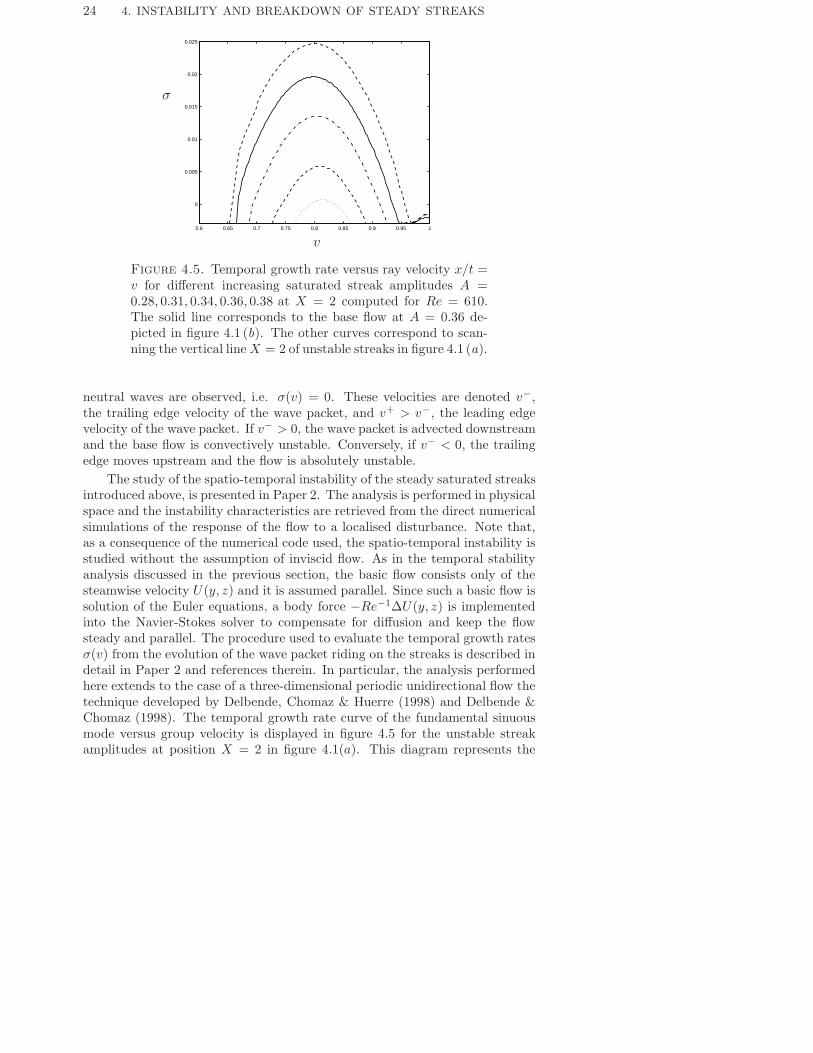
Figure 4.6. Energy in different Fourier modes (ω, β) versusthe Reynolds number. Frequencies: zero (streaks), one (sec-ondary instability), two (higher harmonic). —, β = 0; - - -,β = 1; · · ·, β = 2.

4.3. Streak breakdown

The full transition scenario resulting from the fundamental sinuous instabilityof the steady saturated streaks is presented in Paper 3. The saturated streaksand one of the instability modes of highest spatial growth rate are forced as in-flow perturbation in the fringe region of the numerical code. The direct numer-ical simulation of the streak transition requires extensive computer resourcessince a turbulent flow is induced at the end of the computational domain andthis needs to be fully resolved.

First, the perturbation velocity fields obtained at each streamwise sta-tion are transformed in time and in the spanwise direction to Fourier space.To present the results, the notation (ω, β) is used, where ω and β are thefrequency and spanwise wavenumber each normalised with the fundamentalfrequency and wavenumber of the secondary instability mode. In the presentanalysis we therefore consider the amplitude of the spanwise Fourier compo-nents of the periodic eigenfunction q(y, z) and of its harmonics in time. Thedownstream energy growth in some selected time and spanwise Fourier modesis displayed in figure 4.6. The zero-frequency mode, i.e. the streak, and thesecondary instability (ω = 1) are present at the beginning of the computation,while the higher harmonics (ω > 1) are excited as the flow evolves downstream.Initially the growth is exponential with the growth rate of the first harmonic(ω = 2) twice that of the fundamental mode and similarly, for higher frequen-cies, the growth rate is proportional to the harmonic order (not shown here, seePaper 3). This can be explained by the fact that the nonlinear interaction of

4.3. STREAK BREAKDOWN 27

the fundamental mode q ≈ ei(αx−ωt), the only time-dependent mode initiallyin the flow, with itself gives a forcing term of the type ≈ ei(2αx−2ωt). Thisintroduces in the flow the frequency 2ω with associated spatial growth rate2αi, where αi is the spatial growth rate of the fundamental instability. Thus,in general, the exponential behaviour at a frequency is given by the sum of theexponential of the modes whose interaction gives a contribution at the specificfrequency considered. Hence, in the same way, the mode ω = 3 is induced bythe interaction of the modes ω = 1 and ω = 2 and it has a spatial growthrate that is about 3αi. Thus, at these early stages in the transition process,nonlinear interactions become appreciable. However, one can note that the be-haviour of the most energetic modes (the streak and the secondary instability)is hardly affected by the generation of the higher harmonics. The behavioursof these, in turn, can be explained simply by the interaction of modes of higherenergy. This type of behaviour is usually referred to as weakly nonlinear andit accounts for the simplest type of nonlinear effects; the interaction betweenhigh energy modes induce new harmonics in the flow without affecting theinteracting modes.

It can also be seen in figure 4.6 that the energy content is of the sameorder for modes of different spanwise wave numbers but same frequency. Thisis due to the fact that the streak develops to a highly nonlinear stage before itbecomes unstable to time-dependent disturbances. Therefore the harmonics inβ are generated during the streak growth and they are responsible for the largespanwise shear of the flow. The instability of the streaks is characterised bymodes localised in the spanwise direction so that a number of spanwise wavenumbers is needed to correctly capture it.

The growth in the different modes starts to saturate around position Re =650 and soon the energy become of the same order for the different frequencies.From this point, the weakly nonlinear approximation is no longer valid. In fact,it can be noted in the figure how the energy in the (0, 1) and (0, 2) modes,representing the spanwise modulation of the flow, decreases by a factor of ten,which implies that the streak is disrupted. Conversely, the (0, 0) perturbationmode is growing since the mean laminar velocity profile is approaching itsturbulent counterpart. The late stages of the transition process, before theflow reaches a fully turbulent state, are then analysed in terms of large-scaleflow structures.

Vortical structures can be identified in the flow by plotting regions of lowpressure, or, alternatively, regions where the second largest eigenvalue λ2 ofthe Hessian of the pressure assumes negative values (Jeong et al. 1997). Bothquantities enable to locate regions of strong rotational fluid motion. A top andside view of the flow structures characteristic of the late stages of the sinuousstreak breakdown are shown in figure 4.7. The dark gray isosurfaces representlow-pressure regions while the low-speed streak is depicted with lighter grey.The main structures observed consist of quasi streamwise vortices located onthe flanks of the low-speed streak, which is oscillating in the spanwise direction.


(a)

z

(b)

y

x

Figure 4.7. (a) Top and (b) side view of the structures atthe late stages of transition. Lighter grey represents negativestreamwise velocity perturbation and dark grey regions of lowpressure. In (a) two spanwise streaks are displayed.

Vortices of alternating sign are overlapping in the streamwise direction in astaggered pattern and they are symmetric counterparts, both inclined awayfrom the wall and tilted in the downstream direction toward the middle of theundisturbed low-speed region. The strength and extent of these vortices and thespanwise motion of the low-speed streak increase downstream. It is also evidentfrom the top view that the downstream end of the streamwise vortices, locatedin the outer part of the boundary layer, is tilted in the spanwise direction toform arch vortices.

It is interesting to note that the single streamwise vortex observed in fig-ure 4.7 show similarities to the leg of the Λ-structures seen in transition initiatedby TS-waves (e.g. Rist & Fasel 1995; Bake, Meyer & Rist 2002) and in obliquetransition (Berlin et al. 1999). In fact, in the latter scenarios, positive and neg-ative streamwise vortices are also present on the side of the low-speed regionbut they are not staggered in the streamwise direction. Instead the left andright streamwise vortices join at the centre of the streak and form the typicalΛ-structures. The different relative position of the streamwise vortices is foundto depend on the symmetry of the streamwise vorticity of the secondary insta-bility mode. In the present case, the vorticity disturbance is symmetric, whilein oblique transition and TS-wave induced transition the streamwise vorticityis antisymmetric.

Note finally that the streamwise vortices and streaks are fundamental struc-tures also in the near-wall region of turbulent boundary layers and the vorticesseem to be related to streak instability. In fact, the structures identified as

4.3. STREAK BREAKDOWN 29

typical of the transition of a laminar streak show important similarities withthe streak instability observed in turbulent flows (Jeong et al. 1997; Schoppa& Hussain 2002; Jimenez & Pinelli 1999). On the other hand, the experimentsof Acarlar & Smith (1987) and the related simulations of Skote et al. (2002)among others, show that the appearance of an unstable inflectional wall-normalvelocity profile is a precursor to the formation of horseshoe vortices, thus asso-ciated to the varicose instability of near-wall streaks.

CHAPTER 5

Transition in boundary layers subjected to free-stream

turbulence

Flow visualisations and analogies with transition in vortex-dominated flowsled to believe that transition in boundary layers subjected to free-stream tur-bulence proceeds via the breakdown of the streaks induced inside the bound-ary layer. This motivated the studies presented in the first part of the thesis,where the streak transition is analysed in the simpler case of a steady spanwise-periodic configuration. In this chapter, simulations of a boundary layer sub-jected to free-stream turbulence are presented, where a synthetic turbulentinflow is generated by the procedure outlined in chapter 3. The hypothesisedscenario resulting from the previous studies will find partial confirmation andnew relevant elements will arise. In particular, the present study is focusedupon the receptivity stage and the final breakdown into turbulent spots.

5.1. Receptivity

The occurrence of streamwise elongated structures in boundary layers subjectto free-stream turbulence was first identified by Klebanoff (1971) in terms oflow-frequency oscillations in hot wire signals caused by slow spanwise motionsof the streaks. However, the first theoretical explanations of this phenomenonwere proposed about 25 years later. Bertolotti (1997) has assumed as initialdisturbances vortical modes, solutions of the linearised Navier-Stokes equa-tions in the free stream, which are waves periodic in the spanwise directionand decaying in the streamwise. He has found receptivity to modes with zerostreamwise wavenumber and has shown that the streak growth is connectedto the theories of non-modal growth. Essentially the same linear mechanismfor streak generation caused by the diffusion of a free-stream streamwise vor-tex into the boundary layer has been studied by Andersson et al. (1999) andLuchini (2000) using the boundary layer approximation and by Wundrow &Goldstein (2001) by means of asymptotic expansions. These studies assumethe presence of the vortex at the leading edge show that the growth of thestreak amplitude is proportional to the Reynolds number Re.

Besides these linear models, Berlin & Henningson (1999) have proposed anonlinear mechanism. Numerical simulations have in fact shown that obliquewaves in the free stream can interact to generate streamwise vortices, which,in turn, induce streaks inside the boundary layer. The latter process is further

30

5.1. RECEPTIVITY 31

investigated in this thesis by means of a weakly nonlinear model based ona perturbation expansion of the disturbance truncated at second order. Theperturbation equations are derived directly from the Navier-Stokes equations,superimposing a perturbation field to the base flow, the Blasius profile whichis assumed parallel in the streamwise direction. A single equation is thenobtained for each wavenumber pair (α, β) of the perturbation velocity field.The problem for the first order disturbance velocity and for the second ordercorrection are both governed by the Orr-Sommerfeld and Squire operators.The solution for the first order perturbation velocity is induced by an externalforcing of small amplitude amplitude ε. At second order, O(ε2), the problemis forced by the nonlinear interaction of first order solutions with wavenumberpairs such that their combination is equal to the wavenumber of the mode underconsideration. In particular, the long time response of the boundary layer toa couple of oblique modes of given frequency ω travelling in the free stream isstudied. Oblique modes are associated to (α,±β) modes and their quadraticinteractions produce perturbations of wavenumber (0,±2β), which correspondto streamwise elongated structures.

The results of this analysis are presented in Paper 6, where two types offree-stream perturbations are considered: the first case amounts to the receptiv-ity to oblique waves generated by a wave-like external forcing term oscillating inthe free-stream, the second the receptivity to free-stream turbulence-like dist-urbances, represented as superposition of modes of the continuous spectrumof the Orr-Sommerfeld and Squire operators. In both cases, the generation ofa strong streamwise component of the disturbance in streamwise-independentmodes is the dominant feature. The underlying mechanism can be reduced toa two-step process, first the nonlinear generation of streamwise vorticity forcedby the interactions between disturbances in the free stream and then the for-mation of streaks by the linear lift-up effect. An interesting result is that theimportance of the two steps in the receptivity process is comparable. In fact,the analysis of the equations derived applying the weakly nonlinear approachshows that an amplification of O(Re) occurs both for the generation of thestreamwise vortices and, afterwards, for the formation of streaks. Thus, thestreak growth is of order O(Re2). Recall, however, that the nonlinear mech-anism assumes a forcing of amplitude ε2, i.e. quadratic in the amplitude ofthe free-stream disturbances, in comparison with the stronger direct forcing ofamplitude ε of the linear receptivity models cited above.

The two mechanisms are compared by means of DNS to try to identifywhich of the two can be considered as the most relevant in cases with knownfree-stream perturbations. In order to do so different levels of free-streamturbulence intensity are considered and, moreover, the free-stream turbulencegeneration is manipulated in order to involve few or many modes with very lowvalues of the frequency ω. In this way, we are able to control the amount of low-frequency perturbation part of the inflow turbulence. As shown by Hultgren &Gustavsson (1981) among others, modes of the continuous spectra with very

32 5. TRANSITION UNDER FREE-STREAM TURBULENCE

Rex

urm

s

(a)

4 6 8 10 12

x 104

0

0.02

0.04

0.06

0.08

0.1

0.12

Rex

urm

s

(b)

4 6 8 10 12

x 104

0

0.05

0.1

0.15

0.2

Rex

urm

s/Tu2

(c)

4 6 8 10 12

x 104

0

0.002

0.004

0.006

0.008

0.01

Rex

urm

s/Tu

(d)

4 6 8 10 12

x 104

0

0.01

0.02

0.03

0.04

0.05

Figure 5.1. Streamwise evolution of the wall-normal maxi-mum of urms for three levels of free-stream turbulence inten-sity: - - -, Tu = 4.7%; —–, Tu = 3% and - · -, Tu = 1.5%. Theresults in (a) pertain to the case of few low-frequency modes aspart of the inflow perturbation spectrum, while the data in (b)to a free-stream turbulence spectrum rich with low-frequencymodes. (c): The same rms-values as in (a) are scaled withthe square of the free-stream turbulence intensity Tu. (d):The same rms-values as in (b) are scaled with the free-streamturbulence intensity Tu.

low values of α and ω do not feel the shear layer and they are therefore notzero inside the boundary layer.

The wall-normal maximum of the streamwise velocity perturbation inducedinside the boundary layer is displayed in figure 5.1 versus the local Reynoldsnumber for six cases considered. The results in figure 5.1(a) pertain to three dif-ferent free-stream turbulence levels, Tu = 4.7%, Tu = 3% and Tu = 1.5%, withintegral length scale L = 7.5δ∗0 , where δ∗0 is the boundary-layer displacementthickness at the inlet of the computational domain (Reδ∗

0= 300). For all cases

only few modes characterised by low frequency are introduced as part of theinflow perturbation spectrum. It is shown in figure 5.1(c) that by dividing theurms values in figure 5.1(a) with the square of the turbulence intensity Tu, thegrowth of the perturbation follows, after an initial phase, almost parallel lines.This is more evident in the case of largest intensities. Therefore the dominatingreceptivity mechanism is the nonlinear one (see Paper 7 for more details). Theresults in figure 5.1(b) pertain to cases with the same free-stream turbulencelevels and integral length scale, but this time the perturbation spectrum is

5.2. EFFECT OF THE INTEGRAL LENGTH SCALES 33

characterised by many low-frequency modes, as shown by the high urms-valuesalready at the inlet of the computational domain. In this case, the streaksformed in the boundary layer further downstream are stronger than before; theurms scales linearly with the perturbation intensity Tu (see figure 5.1d) andthe receptivity mechanism responsible for the streak growth is the linear one.From the results in the figure it is possible to conclude that the linear mech-anism is the most relevant if the free-stream turbulence contains significantlow-frequency modes.

5.2. Effect of the integral length scales of the free-streamturbulence

Simulations have then been performed to follow the subsequent breakdown andtransition to turbulence. Results are presented for three cases. In all of themthe inlet of the computational box is at Reδ∗

0= 300 (Rex0 = 30000) and the

free-stream turbulence intensity is 4.7%. Different integral length scales of theinflow turbulence have been used, that is L = 2.5 δ∗0 , L = 5 δ∗0 and L = 7.5 δ∗0where L is related to the longitudinal two-point correlation as L11 = 0.643L.

Rex

cf (×

0.0

01)

laminar

turbulent (a)

100000 200000 3000000

1

2

3

4

5

6

7

Rex

max

imum

urm

s2

(b)

100000 200000 3000000 0

0.5

1

1.5

y /

δ*

Rex

∆ z

min

/ δ*

(c)

100000 200000 300000

1.5

2

2.5

3

3.5

Figure 5.2. (a) Skin friction coefficient, (b) maximum u2rms

(thick lines) and its wall-normal position (thin lines), and (c)first minimum of the spanwise correlation of the streamwisevelocity fluctuations scaled with the local displacement thick-ness δ∗; plotted for L = 7.5δ∗0 (dashed line), L = 5δ∗0 (solidline) and L = 2.5δ∗0 (dash-dotted line).


Some of the data obtained by averaging in time and in the spanwise direc-tion are displayed in figure 5.2. The friction coefficient is shown in figure 5.2(a);also the values for a laminar and a turbulent boundary layer are displayed forcomparison. For the case with the smallest integral length scale transition doesnot occur within the computational domain, while the transition location is atlower Rex for L = 7.5δ∗0 , in agreement with the experimental findings in Jonaset al. (2000). In figure 5.2(b) the maximum u2

rms at each downstream positionis depicted to show the evolution of the streaks. In all cases the energy of thestreaks is proportional to the distance from the leading edge, as observed inthe experiments, and the growth is initially largest in the case of L = 2.5 δ∗0 ,indicating that the smallest scales penetrate easier into the boundary layer.However, this growth can not be sustained as in the other cases. In fact, thefree-stream turbulence decays faster for smaller L and therefore it is less ef-fective in continuously forcing the streaks along the plate. In figure 5.2(a) thewall-normal position of maximum urms is also shown. This is reported in unitsof δ∗, the local boundary-layer displacement thickness. The laminar streakshave a maximum at about y = 1.3δ∗, while their turbulent counterparts arelocated much closer to the wall. In figure 5.2(c) one can see the evolution ofthe first minimum of the spanwise correlation of the streamwise velocity fluc-tuations at the wall normal position of maximum urms; this is a measure ofhalf the spanwise wavelength of the streaks. It can be seen from the figure thatthe length scale of the perturbation inside the boundary layer is only slightlydependent on the free-stream turbulence characteristic scale. The spanwisescales observed are in agreement with the prediction of optimal amplification(Andersson et al. 1999).

5.3. Turbulent spot generation

A snapshot of the flow is shown in figure 5.3 where the instantaneous streamwiseand spanwise velocities are plotted in a plane parallel to the wall. The overallpicture of the transition scenario can be deduced from the figure. Starting fromthe inlet position, the perturbation in the boundary layer appears mainly in thestreamwise velocity component, in the form of elongated structures. Patches ofirregular motion are seen to appear further downstream; these are more evidentin the spanwise component, otherwise very weak in the streaky boundary layer.As they travel downstream, the spots become wider and longer. Note alsothat laminar streaks can be observed downstream of the spots. The turbulentregion at the end of the domain is created by the enlargement and merging ofthe various spots and therefore the streamwise position at which the flow isturbulent varies with time; the turbulent flow is convected downstream and itwould not be seen if new spots were not formed all the time.

The breakdown is analysed in detail by looking at the instantaneous three-dimensional flow configurations for a number of spots, tracing back in timethe location of their formation. An important feature of the spot precursors,observed in all cases considered, is the presence of regions of positive and nega-tive wall-normal and spanwise velocity arranged in a quasi-periodic array. Such

5.3. TURBULENT SPOT GENERATION 35

(a)

z

x

(b)

z

x

Figure 5.3. (a) Instantaneous streamwise velocity and (b)spanwise velocity (bottom figure) in a plane parallel to thewall at y/δ∗0 = 2. The plots are not at the actual scale sincethe domain depicted is 900 units long and 90 units wide interms of δ∗0 . The fringe region is not shown.

quasi regular distribution of the cross-stream velocity components is responsiblefor the observed wavy motions of the streaks preceding the breakdown. Visualinspection of many velocity fields enabled to classify the type of breakdownoccurring on the streaks by considering the spanwise symmetry of the wall-normal and spanwise velocities and their position relative to the underlyingstreak.

The flow structures at the incipient spot stage resemble very much thoseobserved in previous study on the breakdown of steady symmetric streaks, bothin the case of the scenario following a sinuous instability (see Paper 3 in thisthesis) and in the case of a varicose scenario (see the experiments by Asai et al.2002). The similarity with either of the two cases is observed in all spots underconsideration.

In the case of the sinuous breakdown, a single low-speed streak under-goes spanwise antisymmetric oscillations, with strong high-frequency pertur-bation velocity located in the region of largest spanwise shear between thelow- and high-speed streaks. An instantaneous flow configuration for this typeof scenario is displayed in figure 5.4. The characteristic vortical structures,represented in green by negative values of the eigenvalue λ2, consist of quasi-streamwise vortices located on the flanks of the low-speed streak (depictedhere in blue colour). Vortices of alternating sign are overlapping in the stream-wise direction in a staggered pattern, exactly as observed in figure 4.7 for thebreakdown of a periodic array of steady streaks.


In the case of varicose or symmetric breakdown the oscillations of thestreaks are driven by the wall-normal shear and the transition scenario is char-acterised by the appearance of horse-shoe or hairpin structures. An exampleof such vortical structures is displayed in figure 5.5. One can note the forma-tion of hairpin vortices, with pairs of counter-rotating quasi-streamwise vor-tices joining in the middle of the streak, pointing alternatively upstream anddownstream. The streaks generated by free-stream turbulence are obviouslynot symmetric and the perturbations riding on them are not symmetric either;however the velocity components of the high-frequency oscillations show almostthe same pattern with respect to the mean shear of the streaks as in the modelstudies mentioned above. In particular, for the ’quasi-sinuous’ breakdown, itis observed that, for a significant number of spots considered, only streamwisevortices of same sign are clearly identified on one flank of the low-speed region.In these cases, in fact, the spanwise shear is sufficiently high only on one sideof the low-speed streak.

From the analysis of flow visualisations and animations, it is further noticedhow the interaction between low- and high-speed streaks plays an importantrole for the formation of incipient spots. It can be seen in figure 5.5, for example,how the interaction of the low-speed streak with a fast-moving incoming regionof high streamwise velocity is the triggering cause of the instability leading tothe formation of the hairpin vortices. It is observed in experiments (Lundell &Alfredsson 2003) that the streaks are tilted downstream so as the front part islocated in the upper part of the boundary layer whereas the rear part is locatedcloser to the wall. Such a structure is growing in the streamwise directionwhile convected downstream. As a consequence, highly inflectional wall-normalvelocity profiles are induced by the high-speed region when reaching the tail ofthe low-speed region ahead, which thus becomes the site of a local instability.Similarly, the antisymmetric type of breakdown is induced whenever high-speedfluid is approaching a low-speed region on a side. In this case, an inflectionalprofile is forming in the spanwise direction (see figure 5.4). Note also that thestreaks are not perfectly aligned in the streamwise direction but they slowlyoscillates in the boundary layer.

It is finally important to note that the antisymmetric sinuous breakdownis found to be the most likely to occur; it is observed in 16 of the 28 spotsconsidered. From the results presented one may conclude that the breakdownis related to local instabilities associated to the strong shear of the streaks;the fact that almost identical structures are observed in the case of transitioninduced by free-stream turbulence and in the previous model studies on streaksleads to believe that the relevant physics has correctly been captured by thesestudies on the breakdown of steady symmetric streaks.

5.3. TURBULENT SPOT GENERATION 37

x

z

y

Figure 5.4. Instantaneous flow configuration at the break-down of a streamwise streak. Red represents positive pertur-bation streamwise velocity, while blue indicates the low-speedstreak. The green structures are regions of negative λ2, usedto identify vortical structures.

x

y

z

Figure 5.5. Instantaneous flow configuration at the break-down of a streamwise streak. Red represents positive pertur-bation streamwise velocity, while blue indicates the low-speedstreak. The green structures are regions of negative λ2, usedto identify vortical structures.

CHAPTER 6

Conclusions and outlook

The investigations presented in this thesis are motivated by the need to un-derstand bypass transition in boundary layers with high levels of free-streamturbulence. The overall picture of the transition scenario has been elucidated byflow visualisations and velocity measurements in previous experimental studies(see the review articles by Kendall 1998; Matsubara & Alfredsson 2001; Saricet al. 2002). However, some important issues still remain unclear and havebeen the object of the present work. These concern the receptivity stage, dur-ing which perturbations enter the boundary layer, and the mechanisms of thebreakdown into turbulent spots occurring on isolated streaks.

The phenomena under consideration occur randomly in a boundary layersubject to free-stream turbulence and are characterised by a high degree ofintermittency. Therefore, they have first been analysed in detail using simplerflow configurations and known repeatable disturbances. In particular, a weaklynonlinear model for the receptivity of a parallel boundary layer to free-streamdisturbances has been developed. This model provided an efficient tool todisentangle the sequence of events in the receptivity process. This amountsto be a two-step process: the generation of streamwise vortices due to thenonlinear interactions of oblique waves in the free stream, and the formationof streaks by the linear lift-up effect.

The streak instability and breakdown have been studied by consideringspanwise-periodic perturbations resulting from the nonlinear saturation of theoptimal upstream perturbations computed by Andersson et al. (1999) for a nonparallel zero-pressure-gradient boundary layer. The perturbations consideredare steady and optimal only in the linear sense and therefore they representone of several plausible approximations of the streaks observed in boundarylayers subject to relatively high free-stream turbulence levels. However, thewall-normal shape of the linearly optimal disturbance theoretically determinedby Andersson et al. (1999) and Luchini (2000) is found to be remarkably similarto the measured urms values (Matsubara & Alfredsson 2001). The streak canbe regarded, in fact, as a ’pseudo-mode’ triggered in a boundary layer subjectto significant outside disturbances.

The instability of the boundary layer flow perturbed by such streaks hasbeen studied both in the inviscid approximation and considering the effect ofviscosity. A viscous analysis is required to assess the effect of low-amplitudestreaks on the viscous exponential instability of the undisturbed Blasius profile.

38

6. CONCLUSIONS AND OUTLOOK 39

It is found that the two-dimensional TS-waves evolve into three-dimensionalspanwise-periodic viscous instability modes which are damped by increasingthe streak amplitude. Above a certain threshold these waves are quenchedand the boundary layer is thus stable at intermediate streak amplitudes (ofthe order of 20% of the free-stream velocity). However, sinuous antisymmet-ric perturbations are found to become unstable when further increasing thestreak amplitude. This instability is of completely different nature, it is infact of inflectional type and is driven by the spanwise shear of the basic flow.Moreover, this instability is convective with the most unstable waves travellingdownstream at relatively high velocities (of about 80% of the free-stream ve-locity). It is also shown that the sinuous instability can lead the flow directlyinto the turbulent state, the transition scenario being characterised by the ap-pearance of quasi-streamwise vortices alternating in the streamwise directionin a staggered pattern.

Extensive numerical simulations of a boundary layer subjected to free-stream turbulence have then been performed also to confirm the mechanismspredicted by the previous studies. The simulation of a fully transitional bound-ary layer is a formidable task also for the modern supercomputers and thereforeone cannot hope to reproduce as rich parametric studies as in experimentalworks. However, it is possible to correctly reproduce the main features of thetransition scenario under consideration (see Jacobs & Durbin 2001) and, asa consequence, simulations can be designed to investigate specific problems,thus exploiting the advantages of a numerical study. An obvious advantage ofnumerical simulations is that, once the flow has been simulated, all variables,including those difficult to obtain experimentally, are accessible to observationat the same instant. This enabled us to identify the relevant flow structuresat the breakdown, which is not possible in an experiment due to the randomnature of the spot appearance.

The structures at the breakdown are found to be very similar to those ob-served in previous model studies on the breakdown of steady streaks, both forthe sinuous symmetry, which resulted the most likely to occur, and for the vari-cose symmetry (see Asai et al. 2002, for a recent experimental investigation).Hence, one can assume that the relevant physics has correctly been capturedby these studies on the breakdown of steady symmetric streaks.

Further, the numerical methodology used allows to determine and manip-ulate the energy content of the turbulent inflow. In this way, it has been possi-ble to investigate the receptivity mechanism and the effect of the characteristiclength scale of the free-stream turbulence. The relevance of the nonlinear re-ceptivity mechanism proposed could be verified and compared with the linearreceptivity process presented in previous studies (Bertolotti 1997; Anderssonet al. 1999; Luchini 2000).

The direct numerical simulations have also shown the importance of el-ements not considered in the model studies. Probably the most importantconcerns the interaction between the low- and high-speed streaks, which is

40 6. CONCLUSIONS AND OUTLOOK

seen to be the main triggering mechanism of the streak instability. The rele-vance of such interactions was first suggested by Johansson, Alfredsson & Kim(1991) and Landahl (1990) for the case of near-wall turbulent streaks. Thiscould be the object of future investigations, for example assuming simpler andrepeatable initial conditions.

The physical understanding of transition in boundary layers under free-stream turbulence can be used to implement future control strategies. Thefirst experimental studies show that it is possible to reduce the streak growth(Lundell 2003); however, the design of a control system, which is able to detectthe presence of dangerous situation and decide when to act, needs to be im-proved. In the light of the observation above, a successful control strategy mayaim at reducing the streak interaction and can be based on the detection ofthe relative position between streaks (through the gradients of the streamwisevelocity), rather than on their presence or amplitude.

It is also important to note that the similarity between the wall-layerstreaks in turbulent boundary and their instability (Jimenez & Pinelli 1999;Schoppa & Hussain 2002) and the structure observed in transitional boundarylayers. One can speculate that the near-wall streamwise vortices and streaksare driven by the turbulence in the outer part of the boundary layer in thesame way laminar streaks are induced by the free-stream turbulence. As aconsequence, the receptivity stage becomes an important ingredient of the re-generation cycle of near-wall turbulence, together with the streak formation bythe linear lift-up effect and the streak breakdown.

Acknowledgment

First of all I would like to thank Prof. Dan Henningson which made this notonly possible but also enjoyable. Freedom, support, encouragement, guidanceand optimism are indispensable ingredients for any scientific endeavour and hehas spared none of them.

I want to acknowledge all the people at LadHyX for the warm hospitalityduring the six months I had the possibility to spend in Paris. Special thanks toPatrick Huerre and Jean-Marc Chomaz who greatly assisted me when learningabout the absolute instability and to Carlo Cossu.

I also want to thank all the people I worked with during these years: PaulAndersson, Alessandro Bottaro, Donatella Ponziani and Philipp Schlatter; Isurely learned from all of them.

People at the Department provided a nice and friendly atmosphere andI learn to enjoy innebandy and other swedish specialties very much. I wouldlike to thank all the teachers I had during my years at KTH: Arne Johans-son, Henrik Alfredsson, Gustav Amberg, Tony Burden, Anders Dahlkild andLars Soderholm. I also want to name some of my friends and colleagues inStockholm: Janne Pralits, my swedish room-mates Markus Hogberg and Mar-tin Skote, Astrid Herbst, Ori Levin, Jerome Hoepffner, Arnim Bruger, BjornLindgren, Gustaf Martensson, Jens Fransson, Kristian Granne Angele, JuneShiomi, Fredrik Lundell, Davide Medici, Roland Wyberg, Luca Facciolo.

Several friends have contributed to make these Swedish years even more en-joyable: Marco, Claudio, Gianantonio, Francois, Alessandro, Karin, Barbara,Cecilia, Roberto, Dick, Francesca and Torkel, Alessandra and Alessandro, Da-vide and Lena, Rosanna and Flavio, Matteo Luca, the Rissne Slow Motionfootball team, the volleyball team and Hemsparkat innebandy lag.

Grazie ai miei familiari per esserci stati vicini in questi anni.

Tack Giulia, for all din karlek, ditt stod, talamod och hjalp.

41

Bibliography

Acarlar, M. S. & Smith, C. R. 1987 A study of hairpin vortices in a laminarboundary layer. Part 2. Hairpin vortices generated by fluid injection. J. FluidMech. 175, 43–68.

Andersson, P., Berggren, M. & Henningson, D. S. 1999 Optimal disturbancesand bypass transition in boundary layers. Phys. Fluids 11, 134–150.

Arnal, D. & Juillen, J. C. 1978 Contribution experimentale a l’etude de la reptivited’une couche limite laminaire a la turbulence de l’ecoulement general. RapportTechnique 1/5018. ONERA.

Asai, M., Minagawa, M. & Nishioka, M. 2002 The instability and breakdown ofa near-wall low-speed streak. J. Fluid Mech. 455, 289–314.

Bakchinov, A. A., Grek, G. R., klingmann, B. G. B. & Kozlov, V. V. 1995Transition experiments in a boundary layer with embedded streamwise vortices.Phys. Fluids 7, 820–832.

Bake, S., Meyer, D. G. W. & Rist, U. 2002 Turbulence mechanism in Klebanoff-transition: a quantitative comparison of experiment and direct numerical simu-lation. J. Fluid Mech. (459), 217–243.

Berlin, S. & Henningson, D. S. 1999 A nonlinear mechanism for receptivity offree-stream disturbances. Phys. Fluids 11 (12), 3749–3760.

Berlin, S., Wiegel, M. & Henningson, D. S. 1999 Numerical and experimentalinvestigations of oblique boundary layer transition. J. Fluid Mech. 393, 23–57.

Bers, A. 1983 Space-time evolution of plasma instabilities – absolute and convective.In Handbook of Plasma Physics (ed. M. N. Rosenbluth & R. Z. Sagdeev), , vol. 1,pp. 451–517. North-Holland.

Bertolotti, F. P. 1997 Response of the blasius boundary layer to free-stream vor-ticity. Phys. Fluids 9 (8), 2286–2299.

Bertolotti, F. P., Herbert, T. & Spalart, P. R. 1992 Linear and nonlinearstability of the Blasius boundary layer. J. Fluid Mech. 242, 441–474.

Boiko, A. V., Westin, K. J. A., Klingmann, B. G. B., Kozlov, V. V. &

Alfredsson, P. H. 1994 Experiments in a boundary layer subjected to freestream turbulence. part 2. the role of TS-waves in the transition process. J.Fluid Mech. 281, 219–245.

Bottaro, A. & Klingmann, B. G. B. 1996 On the linear breakdown of Gortlervortices. Eur. J. Mech. B/Fluids 15, 301–330.

42

BIBLIOGRAPHY 43

Delbende, I. & Chomaz, J.-M. 1998 Nonlinear convective/absolute instabilities ofparallel two-dimensional wakes. Physics of Fluids 10, 2724–2736.

Delbende, I., Chomaz, J.-M. & Huerre, P. 1998 Absolute and convective insta-bilities in the Batchelor vortex: a numerical study of the linear impulse response.Journal of Fluid Mech. 355, 229–254.

Drazin, P. & Reid, W. 1981 Hydrodynamic Stability . Cambridge Univ. Press.

Ellingsen, T. & Palm, E. 1975 Stability of linear flow. Phys. Fluids 18, 487–488.

Elofsson, P. A., Kawakami, M. & Alfredsson, P. H. 1999 Experiments on thestability of streamwise streaks in plane Poiseuille flow. Phys. Fluids 11, 915–930.

Fasel, H. & Konzelman, U. 1990 Non-parallel stability of flat-plate boundary layerusing the complete Navier-Stokes equations. J. Fluid Mech. 221, 311–347.

Gaster, M. 1975 A theoretical model of a wave packet in a boundary layer over aflat plate. Proc. R. Soc. London, Ser. A 347, 271–289.

Gaster, M. & Grant, I. 1975 An experimental investigation of the formation anddevelopment of a wave packet in a laminar boundary layer. Proc. R. Soc. London,Ser. A 347, 253–269.

Grosch, C. E. & Salwen, H. 1978 The continuous spectrum of the Orr-Sommerfeldequation. Part 1.The spectrum and the eigenfunctions. J. Fluid Mech. 87, 33–54.

Hall, P. & Horseman, N. J. 1991 The linear inviscid secondary instability oflongitudinal vortex structures in boundary-layers. J. Fluid Mech. 232, 357–375.

Henningson, D. S. 1987 Stability of parallel inviscid shear flow with mean spanwisevariation. Tech. Report FFA-TN 1987-57. Aeronautical Research Institute ofSweden, Bromma.

Herbert, T. 1983 Secondary instability of plane channel flow to subharmonic three-dimensional disturbances. Phys. Fluids 26, 871–874.

Herbert, T. & Bertolotti, F. P. 1987 Stability analysis of non parallel boundarylayers. Bull. Am. Phys. Soc. 32, 2079.

Huerre, P. 2000 Open shear flow instabilities. In Perspectives in Fluid Dynamics(ed. G. K. Batchelor, H. K. Moffatt & M. G. Worster), pp. 159–229. CambridgeUniversity Press.

Huerre, P. & Monkewitz, P. A. 1990 Local and global instabilities in spatiallydeveloping flows. Annu. Rev. Fluid Mech. 22, 473–537.

Huerre, P. & Rossi, M. 1998 Hydrodynamic instabilities in open flows. In Hy-drodynamic and Nonlinear Instabilities (ed. C. Godreche & P. Manneville), pp.81–294. Cambridge University Press.

Hultgren, L. S. & Gustavsson, L. H. 1981 Algebraic growth of disturbances in alaminar boundary layer. Phys. Fluids 24 (6), 1000–1004.

Jacobs, R. J. & Durbin, P. A. 2001 Simulations of bypass transition. J. FluidMech. 428, 185–212.

Jeong, J., Hussain, F., Schoppa, W. & Kim, J. 1997 Coherent structures nearthe wall in a turbulent channel flow. J. Fluid Mech. 332, 185–214.

Jimenez, J. & Pinelli, A. 1999 The autonomous cycle of near wall turbulence. J.Fluid Mech. 389, 335–359.

Johansson, A. V., Alfredsson, P. H. & Kim, J. 1991 Evolution and dynamics ofshear-layer structures in near-wall turbulence. J. Fluid Mech. 224, 579–599.

Jonas, P., Mazur, O. & Uruba, V. 2000 On the receptivity of the by-pass transition

44 BIBLIOGRAPHY

to the length scale of the outer stream turbulence. Eur. J. Mech. B/Fluids 19,707–722.

Kachanov, Y. S., Kozlov, V. V. & Levchenko, V. Y. 1977 Noninear developmentof a wave in a boundary layer. Izv. Akad. Nauk SSSR Mekh. Zhid. Gaza 3, 49–58,in Russian.

Kachanov, Y. S. & Tararykin, O. I. 1987 Experimental investigation of a relax-ating boundary layer. Izv. SO AN SSSR, Ser. Tech. Nauk 18.

Kendall, J. M. 1985 Experimental study of disturbances produced in a pre-transitional laminar boundary layer by weak free-stream turbulence. AIAA Pa-per 85, 1695.

Kendall, J. M. 1998 Experiments on boundary layer receptivity to free-streamturbulence. AIAA Paper (98-0530).

Kim, J., Moin, P. & Moser, R. 1987 Turbulence statistics in fully developed channelflow. J. Fluid Mech. 177, 133–166.

Klebanoff, P. S. 1971 Effect of free-stream turbulence on the laminar boundarylayer. Bull. Am. Phys. Soc. 10, 1323.

Klebanoff, P. S., Tidstrom, K. D. & Sargent, L. M. 1962 The three-dimensional nature of boundary layer instability. J. Fluid Mech. 12, 1–34.

Klingmann, B. G. B., Boiko, A., Westin, K. J. A., Kozlov, V. V. & Alfreds-

son, P. H. 1993 Experiments on the stability of Tollmien-Schlichting waves.Eur. J. Mech. B/Fluids 12, 493–514.

Kreiss, H.-O. & Oliger, J. 1972 Comparison of accurate methods for the integra-tion of hyperbolic equations. Tellus XXIV, 199–215.

Landahl, M. T. 1975 Wave breakdown and turbulence. SIAM J. Appl. Maths 28,735–756.

Landahl, M. T. 1990 On sublayer streaks. J. Fluid Mech. 212, 593–614.

Luchini, P. 2000 Reynolds-number independent instability of the boundary layerover a flat surface. Part 2: Optimal perturbations. J. Fluid Mech. 404, 289–309.

Lundbladh, A., Berlin, S., Skote, M., Hildings, C., Choi, J., Kim, J. & Hen-

ningson, D. S. 1999 An efficient spectral method for simulation of incompress-ible flow over a flat plate. Technical Report KTH/MEK/TR–99/11–SE. KTH,Department of Mechanics, Stockholm.

Lundell, F. 2003 Experimental studies of bypass transition and its control. PhDthesis, Royal Institute of Technology, Stockholm, Sweden.

Lundell, F. & Alfredsson, P. H. 2003 Streamwise scaling of streaks in laminarboundary layers subjected to free-stream turbulence. J. Fluid. Mech. Submittedfor publication.

Malik, M. R., Zang, T. A. & Hussaini, M. Y. 1985 A spectral collocation methodfor the Navier-Stokes equations. J. Comp. Phys. 61, 64–88.

Matsubara, M. & Alfredsson, P. H. 2001 Disturbance growth in boundary layerssubjected to free stream turbulence. J. Fluid. Mech. 430, 149–168.

Monkewitz, P. 1988 The absolute and convective nature of instability in two-dimensional wakes at low Reynolds numbers. Phys. Fluids 31 (5), 999–1006.

Morkovin, M. V. 1969 The many faces of transition. In Viscous Drag Reduction(ed. C. S. Wells). Plenum Press.

Nayfeh, A. H. & Mook, D. T. 1979 Nonlinear oscillations. Wiley-Interscience.

Nordstrom, J., Nordin, N. & Henningson, D. S. 1999 The fringe region technique

BIBLIOGRAPHY 45

and the Fourier method used in the direct numerical simulation of spatiallyevolving viscous flows. SIAM J. Sci. Comp. 20, 1365–1393.

Orr, W. M. F. 1907 The stability or instability of the steady motions of a perfectliquid and of a viscous liquid. Part I: A perfect liquid. Part II: A viscous liquid.Proc. R. Irish Acad. A 27, 9–138.

Orszag, S. A. 1972 Comparison of pseudospectral ans spectral approximations. Stud.Appl. Math. 51, 253–259.

Orszag, S. A. & Patera, A. T. 1983 Secondary instability of wall-bounded shearflows. J. Fluid Mech. 128, 347–385.

Park, D. S. & Huerre, P. 1995 Primary and secondary instabilities of the asymp-totic suction boundary layer on a curved plate. J. Fluid Mech. 283, 249–272.

Rayleigh, L. 1880 On the stability of certain fluid motions. Proc. Math. Soc. Lond.11, 57–70.

Reddy, S. C., Schmid, P. J., Baggett, J. S. & Henningson, D. S. 1998 On thestability of streamwise streaks and transition thresholds in plane channel flows.J. Fluid Mech. 365, 269–303.

Rist, U. & Fasel, H. 1995 Direct numerical simulation of controlled transition in aflat-plate boundary layer. J. Fluid Mech. 298, 211–248.

Rogallo, R. S. 1981 Numerical experiments in homogeneous turbulence. Tech. Rep.Tech. Memo. 81315. NASA.

Saric, W. S., Reed, H. L. & Kerschen, E. J. 2002 Boundary-layer receptivity tofreestream disturbances. Annu. Rev. Fluid Mech. 34, 291–319.

Schlichting, H. 1933 Berechnung der anfachung kleiner storungen bei der platten-stromung. ZAMM 13, 171–174.

Schmid, P. J. & Henningson, D. S. 2001 Stability and Transition in Shear Flows.New York: Springer.

Schoppa, W. & Hussain, F. 2002 Coherent structure generation in near-wall tur-bulence. J. Fluid Mech. 453, 57–108.

Schubauer, G. B. & Skramstad, H. F. 1947 Laminar boundary layer oscillationsand the stability of laminar flow. J. Aero. Sci. 14, 69–78.

Skote, M., Haritonidis, J. H. & Henningson, D. S. 2002 Varicose instabilitiesin turbulent boundary layers. Physics of Fluids 14, 2309–2323.

Sommerfeld, A. 1908 Ein beitrag zur hydrodynamischen erklarung der turbulentenflussigkeitbewegungen. In Atti. del 4. Congr. Internat. dei Mat. III, Roma, pp.116–124.

Swearingen, J. D. & Blackwelder, R. F. 1987 The growth and breakdown ofstreamwise vortices in the presence of a wall. J. Fluid Mech. 182, 255–290.

Tollmien, W. 1929 Uber die entstehung der turbulenz. Nachr. Ges. Wiss. Gottingen21-24, English translation NACA TM 609, 1931.

Waleffe, F. 1995 Hydrodynamic stability and turbulence: Beyond transients to aself-sustaining process. Stud. Appl. Math. 95, 319–343.

Waleffe, F. 1997 On a self-sustaining process in shear flows. Phys. Fluids 9, 883–900.

Westin, K. J. A., Boiko, A. V., Klingmann, B. G. B., Kozlov, V. V. &

Alfredsson, P. H. 1994 Experiments in a boundary layer subject to free-stream turbulence. part i: Boundary layer structure and receptivity. J. FluidMech. 281, 193–218.

46 BIBLIOGRAPHY

Wundrow, D. W. & Goldstein, M. E. 2001 Effect on a laminar boundary layer ofsmall-amplitude streamwise vorticity in the upstream flow. J. Fluid Mech. 426,229–262.

Date post:	09-Jul-2018
Category:	Documents
Upload:	buithuan
View:	224 times
Download:	0 times

Numerical studies of bypass transition in the Blasius ...9331/FULLTEXT01.pdf · Numerical studies...

Documents