Topology and its Applications 93 (1999) 219–259 The boundary of the Gieseking tree in hyperbolic three-space R.C. Alperin a,1 , Warren Dicks b,*,2 , J. Porti c,2 a Department of Mathematics and Computer Science, San Jose State University, San Jose, CA 95192-0103, USA b Departament de Matem` atiques, Universitat Aut` onoma de Barcelona, 08193 Bellaterra (Barcelona), Spain c Laboratoire Emile Picard, CNRS UMR 5580, Universit´ e Paul Sabatier, 31062 Toulouse Cedex 4, France Received 20 March 1997; received in revised form 10 October 1997 Abstract We give an elementary proof of the Cannon–Thurston Theorem in the case of the Gieseking manifold. We do not use Thurston’s structure theory for Kleinian groups but simply calculate with two-by-two complex matrices. We work entirely on the boundary, using ends of trees, and obtain pictures of the regions which are successively filled in by the Peano curve of Cannon and Thurston. 1999 Elsevier Science B.V. All rights reserved. Keywords: Gieseking manifold; Cannon–Thurston map; Ends of topological spaces AMS classification: Primary 57M60, Secondary 57M50 1. Introduction The Gieseking manifold M is the three-manifold fibred over the circle S 1 with fibre F a punctured torus, and with homological monodromy ( 01 11 ) . This monodromy determines the manifold M , which is unorientable, and hyperbolic, with an unoriented cusp. Let H n denote n-dimensional hyperbolic space. Its boundary, ∂H n , is homeomorphic to the (n - 1)-sphere S n-1 , and its compactification, H n ∪ ∂H n , is homeomorphic to the closed n-ball. The hyperbolic structure of the Gieseking manifold, M , induces a homeomorphism between the universal cover, f M , and H 3 . In particular, we have an action of π 1 (M ) on H 3 . Since the fibre F is a punctured torus, it admits finite-volume complete hyperbolic * Corresponding author. E-mail: [email protected]. 1 Partially supported by the National Security Agency (USA). 2 Partially supported by the DGICYT (Spain) through grant number PB93-0900. 0166-8641/99/$ – see front matter 1999 Elsevier Science B.V. All rights reserved. PII:S0166-8641(97)00270-8
Transcript
Topology and its Applications 93 (1999) 219–259
The boundary of the Gieseking tree in hyperbolic three-space
R.C. Alperin a,1, Warren Dicks b,∗,2, J. Porti c,2
a Department of Mathematics and Computer Science, San Jose State University, San Jose,CA 95192-0103, USA
b Departament de Matematiques, Universitat Autonoma de Barcelona, 08193 Bellaterra (Barcelona), Spainc Laboratoire Emile Picard, CNRS UMR 5580, Universite Paul Sabatier, 31062 Toulouse Cedex 4, France
Received 20 March 1997; received in revised form 10 October 1997
Abstract
We give an elementary proof of the Cannon–Thurston Theorem in the case of the Giesekingmanifold. We do not use Thurston’s structure theory for Kleinian groups but simply calculate withtwo-by-two complex matrices. We work entirely on the boundary, using ends of trees, and obtainpictures of the regions which are successively filled in by the Peano curve of Cannon and Thurston. 1999 Elsevier Science B.V. All rights reserved.
Keywords: Gieseking manifold; Cannon–Thurston map; Ends of topological spaces
The Gieseking manifold M is the three-manifold fibred over the circle S1 with fibre Fa punctured torus, and with homological monodromy
(0 11 1
). This monodromy determines
the manifold M , which is unorientable, and hyperbolic, with an unoriented cusp.Let Hn denote n-dimensional hyperbolic space. Its boundary, ∂Hn, is homeomorphic
to the (n− 1)-sphere Sn−1, and its compactification, Hn ∪ ∂Hn, is homeomorphic tothe closed n-ball.
The hyperbolic structure of the Gieseking manifold, M , induces a homeomorphismbetween the universal cover, M , and H3. In particular, we have an action of π1(M) onH3. Since the fibre F is a punctured torus, it admits finite-volume complete hyperbolic
∗ Corresponding author. E-mail: [email protected] Partially supported by the National Security Agency (USA).2 Partially supported by the DGICYT (Spain) through grant number PB93-0900.
0166-8641/99/$ – see front matter 1999 Elsevier Science B.V. All rights reserved.PII: S0166-8641(97)0 02 70 -8
220 R.C. Alperin et al. / Topology and its Applications 93 (1999) 219–259
structures. Such a hyperbolic structure on F induces a homeomorphism between theuniversal cover, F , and H2. So every lift of the embedding of F into M induces anembedding of H2 into H3, which is π1(F )-equivariant.
We give an elementary proof of the Cannon–Thurston Theorem in the particular caseof the Gieseking manifold, and hence all finite covers thereof, such as the complementof the figure-eight knot.
Theorem A (Cannon and Thurston [2]). Every lift to the universal cover of the embed-ding F → M induces an embedding H2 → H3 which extends continuously to aπ1(F )-equivariant quotient map Ψ :∂H2 → ∂H3.
By a quotient map, we mean a surjective map between topological spaces, such that thetopology of the image space agrees with the resulting quotient topology, so, in particular,the map is continuous.
We remark that, at the time of writing, [2] leaves the cusped case of the Cannon–Thurston Theorem to the reader, while both [2] and [9] give proofs of the cuspless case.In contrast, our arguments are highly specific to the Gieseking example; with more workwe could have included also the similar case where the homological monodromy is
(0 11 2
),
but, beyond that, some of our techniques do not seem to apply.Let G be the group with presentation 〈a, b, c | a2 = b2 = c2 = 1〉, and TG the Cayley
graph for this presentation, with oriented edges paired off to form unoriented edges. ThenTG is an unoriented tree whose vertices are trivalent; see Fig. 3. The set of ends of TGis called the boundary of TG, and is denoted ∂TG. The fundamental group π1(F ) of thefibre embeds as a subgroup of index two in G.
We prove Theorem A by considering two G-equivariant maps from TG, one into H2,and the other into H3, which can be extended to maps from ∂TG to ∂H2, and to ∂H3,respectively.
First we define an action of G on H2 ∪ ∂H2. We set
a(x) =−1/x,
b(x) = (x− 1)/(2x− 1),
c(x) = (x− 2)/(x− 1),
for each x in the completed real line R = R ∪ {∞}, with the usual conventions aboutinfinity. This defines an action of G on R by Mobius transformations, and we identify∂H2 with R. The resulting isometric action of G on H2 is discrete and faithful; seeSections 3.2 and 3.3. The ideal triangle δ of H2 having vertices 0, 1, and ∞ in ∂H2
is a fundamental domain for the action of G. The G-translates of δ determine an idealtessellation of H2 called the Farey tessellation; see, for example, [12]. The quotientG\H2 is a hyperbolic orbifold doubly covered by a punctured torus.
Notice that specifying a point of H2 as the image of the identity vertex of G isequivalent to specifying a G-equivariant map TG →H2.
R.C. Alperin et al. / Topology and its Applications 93 (1999) 219–259 221
Proposition B. There exists a G-equivariant quotient map τ :∂TG → ∂H2 which con-tinuously extends any G-equivariant map TG →H2.
Next, we define an action of G on H3 ∪ ∂H3. We set
a(z) =−1/z,
b(z) = (z − 1)/((ω + 1)z − 1),
c(z) = (z − (ω + 1))/(z − 1),
for every z in the Riemann sphere C = C ∪ {∞}, where ω = exp(2πi/3), and weuse the standard conventions about infinity. This defines a G-action on C by Mobiustransformations, and we identify ∂H3 with C. Again, the resulting isometric action ofG on H3 is discrete and faithful; see Sections 7.1 and 8.11.
Let us describe how this action comes from the hyperbolic structure of the Giesekingmanifold. Let γ1 and γ2 be free generators of the fundamental group π1(F ) of the fibre,F , and let θ be the automorphism of π1(F ) such that θ(γ1) = γ−1
1 and θ(γ2) = γ−12 .
Then G can be viewed as the semidirect product of π1(F ) with the group of order twogenerated by the involution θ via the isomorphism:
γ1 ↔ ca, γ2 ↔ cb, θ↔ c.
Since θ is in the center of the outer automorphism group of π1(F ), it induces an involutionof π1(M). So, by Mostow’s Rigidity Theorem, G acts isometrically on H3, and theπ1(F )-action induced by the G-action is the restriction of the holonomy representationof π1(M). This π1(F )-action was studied in detail by Jørgensen and Marden [7].
Theorem C. There exists a G-equivariant quotient map Φ :∂TG → ∂H3 which con-tinuously extends any G-equivariant map TG → H3. Moreover, Φ factors through themap τ :∂TG → ∂H2 given by Proposition B, to give a G-equivariant quotient mapΦ :∂H2 → ∂H3.
In light of Proposition B, Theorem C follows easily from Theorem A, but we willuse the former to prove the latter. The map Φ of Theorem C has the property of the Ψof Theorem A, because our G-action on H2 arises from a suitable hyperbolic structureon F .
We recall that a Jordan curve in S2 is a simple closed curve, and a Jordan regionis a closed subset of S2 with nonempty interior whose boundary is a Jordan curve. Bya Jordan partition of S2 we mean a finite set of Jordan regions, with pairwise disjointinteriors, whose union is all of S2; similarly, a Jordan partition of a Jordan region R ofS2 is a finite set of Jordan regions, with pairwise disjoint interiors, whose union is allof R.
The proof of Theorem C is based on the next result which gives the Jordan partitionof C depicted in Fig. 1.
222 R.C. Alperin et al. / Topology and its Applications 93 (1999) 219–259
(a)
(b)
Fig. 1. The Jordan partition of the Riemann sphere C. (a) Front. (b) Back.
Theorem D. There exist three Jordan regions Ra, Rb, and Rc in ∂H3 = C, withpairwise disjoint interiors, satisfying the following.
(0) C = Ra ∪Rb ∪Rc.(1) aRa = Rb ∪Rc.(2) bRb = Ra ∪Rc.(3) cRc = Ra ∪Rb.
R.C. Alperin et al. / Topology and its Applications 93 (1999) 219–259 223
The map Φ of Theorem C will be constructed by using Theorem D to create a tree ofsubsets as follows. We define a map from the set of vertices of TG to the set of subsetsof C. We start with the base vertex 1, which we make correspond to the whole Riemannsphere C. Next we make the vertices adjacent to 1, namely a, b, and c, correspond toRa, Rb, and Rc, respectively. The vertices adjacent to a, other than 1, are ab and ac,which we make correspond to aRb and aRc, respectively, and these are contained in Ra,by (1). In a similar way, we make aba correspond to abRa, which is contained in aRb,and so on.
Given an end e ∈ ∂TG, we view e as a right infinite reduced word in a, b, c, thatis, a reduced word which extends infinitely to the right. We also view e as the limit ofthe increasing sequence of its finite initial words, and this sequence corresponds to adecreasing sequence of subsets of C. We will show that the intersection of this sequenceof subsets is a set which contains a single point, which we then define to be Φ(e).
From this construction, if [a] ⊂ ∂TG denotes the set of right infinite reduced wordsstarting with a, then Ra = Φ[a]; and similarly with b, or c, in place of a.
We then will obtain the following as a consequence.
Corollary E. Let Φ :∂H2 → ∂H3 be the map given by Theorem C. For any p, q, r, s ∈ Zsuch that ps− qr = ±1, Φ([p/q, r/s]) and Φ(∂H2− [p/q, r/s]) form a Jordan partitionof ∂H3.
We remark that ∂H3 decomposes as a union of four regions aRb, aRc, Rb, and Rc,and these are transitively permuted by the Mobius transformations a(z) = −1/z, andd(z) = 1/z. Further, a and d have a common fixed point in H3, so if this fixed point istaken as the centre of the ball, as in Fig. 1, a and d act as isometries on ∂H3. Althoughwe shall not do so, one can show that the pairwise overlaps of the four regions havearea zero, so each region has area one quarter the surface area of the sphere. The imageunder ab (respectively ac, ba, ca) of Rb (respectively Rc, bRa, cRa) is the union ofthe three other regions, so the area gets tripled. This is a particularly illustrative exampleof the ‘paradoxical decompositions’ studied by Culler and Shalen [4], corresponding tothe Kleinian group generated by the actions of ab and ac on H3; here Lebesgue measureon ∂H3 decomposes as a sum of four measures, given by Lebesgue measure restrictedto each of our four regions. One can show that for each point z of H3, ab or ac movesz a distance of at least log(2 +
√3 ), slightly more than the value of log(3) guaranteed
by the general results of [4] obtained using paradoxical decompositions.The paper is organized as follows. In Section 2, we recall some definitions about trees
and their boundaries, and we introduce the two examples of trees we shall work with. InSection 3, we introduce the Farey tessellation, which we then use in Section 4 to proveProposition B. In Section 5, we prove a similar proposition for another tree in a convexsubspace of H2. In Sections 6 and 7, we prove some useful lemmas about hyperbolicthree-space and the action of PGL2(Z[ω]), where ω = exp(2πi/3). Theorems C andD, and Corollary E, are proved in Sections 8 and 9. Finally, in Section 11, we proveTheorem A, by using results about the action of PGL2(Z[ω]), proved in Section 10.
224 R.C. Alperin et al. / Topology and its Applications 93 (1999) 219–259
2. Trees and their boundaries
In this section we recall some definitions, and describe the method of constructingmaps from the boundary of a tree by using trees of subsets of a set.
Definitions 2.1. Let T be a locally-finite tree, that is, T is a locally-compact one-dimensional simply-connected CW-complex. We can view T as a combinatorial objector as a metric space, where every edge is isometric to the length one segment [0, 1].
The set of vertices of T is denoted V (T ).From the combinatorial point of view, a ray of T is an infinite sequence of distinct
vertices v0, v1, . . . such that vn is joined to vn+1 by an edge; we then say that the raystarts at v0. In metric terms, a ray is an isometric map r : [0,+∞)→ T , and it starts atr(0).
Two rays v0, v1, . . . and w0, w1, . . . are said to be equivalent if there exist m0, n0 ∈ Zsuch that vm0+n = wn for each n > n0. From the metric point of view, two rays[0,+∞)→ T are equivalent if the symmetric difference of their images lies in a compactset.
An end of T is an equivalence class of rays of T under this equivalence relation.Let v0 be a distinguished vertex of T . Every end is represented by a unique ray starting
at v0. For every vertex w of T , let [w] denote the set of ends represented by rays startingat v0 and passing through w. The boundary of T , denoted ∂T , is the topological spacewhose points are the ends of T , in which {[w] | w ∈ V (T )} is a basis for the opentopology. This topology does not depend on the choice of the distinguished vertex v0.
The union T ∪ ∂T is called the compactification of T and is topologized as follows.For w ∈ V (T ), the shadow of w is the set of points in T that belong to a ray starting at v0
and passing throughw and that are not between v0 and w. As a basis for the open topologyof T ∪ ∂T we take the open sets of T and the family {[w] ∪ shadow(w) | w ∈ V (T )},where shadow(w) denotes the shadow of w. It is easily checked that this induces thepreviously specified topologies on T , and ∂T , and that T ∪ ∂T is compact.
The reader can find further information on ends of trees in Section IV.6 of [5].
Definition 2.2. Let X be a set. We write P(X) to denote the set of all subsets ofX . A tree of subsets of X is a tree T with a distinguished vertex v0, and a mapσ :V (T )→ P(X) such that, if w lies between v0 and v, then σ(v) ⊆ σ(w).
When we described the topology of ∂T , we constructed a tree of subsets w 7→ [w].
Definition 2.3. Let X be a metric space, and T a tree with distinguished vertex v0.A tree of subsets σ :V (T ) → P(X) is contracting if, for every ray v0, v1, v2, . . . , thediameter of σ(vn) tends to zero as n goes to infinity.
Proposition 2.4. Let X be a compact metric space, T a tree with distinguished vertexv0, and σ :V (T )→ P(X) a tree of subsets of Xsuch that σ(v) is nonempty and closed
R.C. Alperin et al. / Topology and its Applications 93 (1999) 219–259 225
for every v ∈ V (T ). Let each end e of T be represented by a ray v0(e), v1(e), . . . ofvertices of T . If σ is contracting, then
⋂n>0 σ(vn(e)) consists of a single point and the
function φ : e 7→⋂n>0 σ(vn(e)) defines a continuous map φ :∂T → X .
Proof. Since all the σ(vn) are compact, and the sequence of their diameters tends tozero, φ :∂T → X is a well-defined map. It remains to check that it is continuous. Letv0, v1, . . . be a ray representing the end e ∈ ∂T . For every ε > 0, there is a nonnegativeinteger n0 such that, for all n > n0, σ(vn) is contained in the ball Bε(φ(e)) with centerφ(e) and radius ε; that is what it means for σ to be contracting. In particular, for alln > n0, the open subset [vn] is contained in φ−1Bε(φ(e)), because φ([vn]) is containedin σ(vn). 2
Notation 2.5. We will be working with two different situations where we have a monoidS, and a tree TS with vertex set S, and distinguished vertex 1.
Definitions 2.6. We write B to denote a free monoid of rank two, and write {f, g} todenote its (unique) free generating set.
Thus the elements of B are the finite words in f and g, including the empty word 1,without any cancellation rule.
Let TB be the Cayley graph for B, as in Fig. 2. Since 1 is the distinguished vertex,every end is represented by a unique right infinite word in f and g.
Assume now that we have a continuous action of B on a compact metric space X . Thisis equivalent to specifying two continuous maps from X to itself, because B is a freemonoid. We then define a B-equivariant tree of closed subsets σ :B = V (TB)→ P(X),by setting σ(w) = w(X) for every w ∈ B. Thus, if σ is contracting, the induced mapφ :∂TB → X is B-equivariant.
Fig. 2. The tree TB with vertex set B.
226 R.C. Alperin et al. / Topology and its Applications 93 (1999) 219–259
Definitions 2.7. Recall from the Introduction that G denotes the group with presentation〈a, b, c | a2 = b2 = c2 = 1〉, so G is isomorphic to the free product C2 ∗ C2 ∗ C2, whereC2 denotes the order two (cyclic) group.
The edges of the Cayley graph for this presentation are paired, since for each edgethere is another edge joining the same two vertices, but going in the opposite direction.We treat each such pair of oriented edges as a single unoriented edge, and so obtain atree TG with vertex set G, as in Fig. 3. Each vertex is trivalent.
As 1 is the distinguished vertex, every end is represented by a right infinite reducedword in a, b and c. (Recall that a word in a, b and c is reduced if any two consecutiveletters are different, that is, all occurrences of a2, b2 and c2 are cancelled.)
Now suppose that G acts continuously on a compact metric space X . Suppose alsothat we have three closed subsets Ra, Rb, and Rc of X satisfying the following:
(0) X = Ra ∪Rb ∪Rc;(1) aRa = Rb ∪Rc;(2) bRb = Ra ∪Rc;(3) cRc = Ra ∪Rb.
We now proceed to define a tree of subsets σ :V (TG) = G→ P(X). We set σ(1) = X ,and, for any nontrivial w ∈ G, we set σ(w) = wdRd where d ∈ {a, b, c} is the last letterof w, when written as a reduced word. It follows from (1)–(3) that σ is a tree of subsets.
When X = ∂TG, if we take Ra = [a], Rb = [b], and Rc = [c], then (0)–(3) aresatisfied:
Fig. 3. The tree TG with vertex set G = 〈a, b, c | a2 = b2 = c2 = 1〉.
R.C. Alperin et al. / Topology and its Applications 93 (1999) 219–259 227
Thus we have a natural tree of subsets of ∂TG.
Proposition 2.8. Let X be a compact metric space and σ :V (TG) = G→ P(X) a treeof subsets as in Definition 2.7. If σ is contracting, then the induced map φ :∂TG → X
is a G-equivariant quotient map.
Proof. The map φ is surjective, since equality holds in (0)–(3). Moreover, φ maps closedsubsets of ∂TG to closed subsets of X , because ∂TG is compact and X is Hausdorff.Thus φ is a quotient map.
The map φ is G-equivariant because σ has the property that, for all v, w ∈ G, if w isnot completely cancelled in vw, then σ(vw) = vσ(w). 2
3. The Farey tessellation of H2
In this section we describe the Farey tessellation, and the action of G on H2.
Definitions 3.1. Recall that H2 denotes the hyperbolic plane, and ∂H2 its boundary.We identifyH2 with the half-plane {z ∈ C | Im(z) > 0}, and ∂H2 with the completed
real line R = R ∪ {∞}.The isometry group of H2 is naturally isomorphic to the group of Mobius transfor-
mations of ∂H2, as follows. Each isometry of H2 extends continuously to H2 ∪ ∂H2
in a unique way, and the resulting action on ∂H2 is a Mobius transformation. Moreoverevery Mobius transformation of ∂H2 arises in this way, from a unique isometry. Thegroup of orientation-preserving Mobius transformations of R is isomorphic to PSL2(R).We represent elements of PSL2(R) in the form ±
(a bc d
), and such an element corresponds
to the isometry and Mobius transformation
z 7→ az + b
cz + d
for all z ∈H2 ∪ ∂H2, with the usual conventions about infinity.For any subset X of ∂H2, the convex hull of X is the smallest convex subset of H2
containing X in its closure.An ideal triangle in H2 is a finite volume triangle whose vertices lie in ∂H2; that is,
an ideal triangle is the convex hull of three points of ∂H2.The Farey tessellation of H2 is a tessellation by ideal triangles with vertices lying in
Q ∪ {∞}, as in Fig. 4. (Here, and throughout, we will usually depict the upper half-plane as a disc, via a conformal transformation.) Two rational numbers p/q and r/s inlowest terms (allowing also ∞ = ±1/0) are joined by an edge in the Farey tessellationif and only if ps− qr = ±1. Every edge having vertices p/q and r/s is adjacent to thetriangles obtained by adding in the vertices (p+ r)/(q + s) and (p− r)/(q − s). Usingthe Euclidean algorithm, one can prove that this defines a tessellation; see [12]. It is clearthat the Farey tessellation is preserved by the action of PSL2(Z).
228 R.C. Alperin et al. / Topology and its Applications 93 (1999) 219–259
Fig. 4. The Farey tessellation of H 2.
Definitions 3.2. Consider the action of G = 〈a, b, c | a2 = b2 = c2 = 1〉 on H2 whichwe described in the Introduction. This action is defined by mapping generators of G toPSL2(Z) as follows:
a 7→ ±(
0 −11 0
), b 7→ ±
(1 −12 −1
), c 7→ ±
(1 −21 −1
).
Since the image lies in PSL2(Z), the G-action is discrete and preserves the Fareytessellation. Notice that a (respectively b, respectively c) acts as an order two rotationaround a point in the edge with vertices 0 and ∞ (respectively 0 and 1, respectively 1and ∞).
Let δ denote the ideal triangle of the Farey tessellation having vertices 0, 1 and ∞.By Poincare’s Theorem [6], we have the following.
Lemma 3.3. The G-action on H2 is faithful, and has δ as a fundamental domain.
Definitions 3.4. The dual tree of the Farey tessellation is the tree whose vertices are theideal triangles of this tessellation, in which two vertices of the dual tree are joined byan edge if and only if the corresponding triangles have a common edge. It follows, fromLemma 3.3, that the dual tree of the Farey tessellation is isomorphic to our Cayley graphTG. Given a point x in the interior of δ, the map
g ∈ G 7→ g(x) ∈H2
R.C. Alperin et al. / Topology and its Applications 93 (1999) 219–259 229
Fig. 5. A copy of TG in H 2.
induces a G-equivariant embedding i : TG → H2 which realizes the isomorphism be-tween TG and the dual tree of the Farey tessellation; see Fig. 5.
We end this section by recording a result from hyperbolic geometry which we will useto study extensions to boundaries. It is well known and easy to prove.
Lemma 3.5. Let (In)n∈N be a decreasing sequence of intervals in R, whose lengths tendto zero, and whose intersection is a singleton {x∞}. Let (xn)n∈N be a sequence in H2.If, for each n ∈ N, xn is contained in the convex hull of In, then the sequence of thexn tends to x∞.
4. The breakup of R
In this section we prove Proposition B, and use the Farey tessellation to construct themap τ :∂TG → ∂H2.
4.1. Proof of Proposition B. We shall show that there exists a map τ :∂TG → ∂H2
which is the continuous extension of a G-equivariant map i : TG →H2. We first constructτ , and then consider i. We define τ by applying Proposition 2.4 to a contracting tree ofsubsets of ∂H2. Consider the following subsets of R = ∂H2:
Ra = [−∞, 0], Rb = [0, 1], Rc = [1,+∞].
230 R.C. Alperin et al. / Topology and its Applications 93 (1999) 219–259
It is easily checked that these subsets satisfy (0)–(3), because their end-points are thevertices of the fundamental domain δ. By Definition 2.7, this choice of Ra, Rb, and Rcdefines a tree of subsets σ :V (TG) → P(∂H2). Thus σ(1) = R, σ(a) = Ra, σ(b) =
Rb, σ(c) = Rc, σ(ab) = aRb, and so on.
Lemma 4.2. The tree of subsets σ :V (TG)→ P(∂H2) is contracting.
Proof. For every vertex v ∈ V (TG) = G, the set σ(v) is an interval of R whose end-points are the ideal vertices of an edge of the Farey tessellation. That is, σ(v) = [p/q, r/s]
for certain p, q, r, s ∈ Z such that ps− qr = ±1. This implies that the length of σ(v) iseither infinite, or the inverse of an integer, because r/s− p/q = ±1/qs. Moreover if thelength of σ(v) is infinite, σ(v) is either [−∞,m] or [m,+∞], for some m ∈ Z.
Let v0, v1, . . . be a ray in TG starting at v0 = 1. The sequence of intervals (σ(vn))n∈Nis strictly decreasing, and the lengths are inverses of integers or infinite. Thus, except inthe case where ∞ is contained in σ(vn) for each n > 0, the sequence of lengths of theσ(vn) tends to zero. When∞ ∈ σ(vn), either σ(vn) is of the form [−∞,mn] and mn isa decreasing sequence of integers, or it is of the form [mn,+∞] and mn is an increasingsequence of integers. In both cases, for any Riemannian metric of R, the sequence oflengths of the σ(vn) tends to zero. 2
4.3. We return to the proof of Proposition B.Since σ is contracting, Proposition 2.4 implies that we get a continuous G-equivariant
map τ :∂TG → ∂H2, which is a quotient map by Proposition 2.8.Let i : TG →H2 be any G-equivariant map. Let (vn)n∈N be a sequence of vertices ofTG with limit an end e ∈ ∂TG. We claim that the sequence of i(vn) tends to τ(e). ByG-equivariance, i(vn) = vni(1), and we recall that 1 is the distinguished vertex of TG.We may assume that i(1) ∈ δ, because the convergence of the sequence (vn(x))n∈N,and its limit, is independent of the point x ∈ H2. Since i(1) ∈ δ, i(vn) ∈ vnδ, soi(vn) belongs to the convex hull of σ(vn). Since σ is contracting, and
⋂n∈N σ(vn) =
{τ(e)}, the sequence of i(vn) tends to τ(e), by Lemma 3.5. This completes the proof ofProposition B. 2
Lemma 4.4. The map τ :∂TG → R of 4.3 is finite-to-one. The preimage τ−1(ξ) has twopoints if ξ ∈ Q ∪ {∞}, and one point if ξ ∈ R−Q.
Proof. Let ξ ∈ R−Q and e ∈ ∂TG such that τ(e) = ξ. We claim that e is unique. Letv0, v1, . . . be the unique ray in TG starting at v0 = 1, and representing e. The vertex v1
is determined by whether ξ belongs to σ(a) = Ra = [−∞, 0], σ(b) = Rb = [0, 1], orσ(c) = Rc = [1,+∞], and the choice of a, b, or c is forced, because ξ is irrational.Similarly, for each n ∈ N, there is only one vertex vn in TG at distance n from v0 = 1such that ξ ∈ σ(vn), because ξ is irrational. We conclude that vn is uniquely determinedby ξ for every n, and, hence, so is e.
If ξ is rational or infinity, it is clear that, for all n ∈ N, there are at most two verticesvn and v′n at distance n from v0 = 1 such that σ(vn) and σ(v′n) contain ξ; since ξ is a
R.C. Alperin et al. / Topology and its Applications 93 (1999) 219–259 231
vertex in the Farey tessellation, there do exist two such vertices if n is sufficiently large.In a ray v0, v1, . . . , the vertices v0 and vn determine the vertices in between them, sothere are exactly two ends in the preimage of ξ. 2
We write (abc)∞ to denote the right infinite word abcabc · · ·, viewed as an end of TG,and similarly for (cba)∞.
Proposition 4.5. Let G act continuously on a topological space X , and let h :∂TG → X
be a continuous G-equivariant map. Then h factors through the map τ :∂TG → R of 4.3,to give a continuous map h :R→ X , if and only if h((abc)∞) = h((cba)∞).
Proof. Direct calculation shows that abc(x) = x− 3 for all x ∈ R. Thus ∞ ∈ R is theonly fixed point of abc. Since τ is G-equivariant, and (abc)∞ is fixed by abc, we see thatτ((abc)∞) = ∞. But the same holds for cba = (abc)−1, so τ((abc)∞) = τ((cba)∞).Hence, if h factors through τ , then h((abc)∞) = h((cba)∞).
Now suppose that h((abc)∞) = h((cba)∞).We claim that for every rational ξ there exists w ∈ G such that ξ = w(∞). Since the
dual tree of the Farey tessellation is isomorphic to TG, there exists w′ ∈ G such that ξis a vertex of the ideal triangle w′(δ), where δ is the ideal triangle with vertices 0, 1,∞.Moreover a(0) = c(1) =∞, so there exists w ∈ G with ξ = w(∞).
From the previous paragraph, and the G-equivariance of τ and h, we deduce that hfactors through a map h :R→ X , which is continuous because τ is a quotient map. 2
5. The breakup of [0,+∞]
In this section, we describe an action of B on [0,+∞], where B is the free monoiddefined in Section 2.6, and we study a B-equivariant map ν :∂TB → [0,+∞], using theFarey tessellation.
Notation 5.1. Let H2+ denote the convex hull of [0,∞] in H2, and consider the restric-
tion of the Farey tessellation to H2+, as in Fig. 6.
Consider the action of B on H2+ ∪ [0,∞] in which the free generators act by f(x) =
x+ 1, g(x) = x/(x+ 1), for all x ∈ [0,∞]; this corresponds to
f 7→ ±(
1 10 1
)and g 7→ ±
(1 01 1
).
Since f([0,∞]) = [1,∞], and g([0,∞]) = [0, 1], are contained in [0,∞], and the two±-matrices belong to PSL2(Z), the B-action respects the restriction of the Farey tessel-lation to H2
+.
Lemma 5.2. The ideal triangle δ which has vertices 0, 1, and ∞ is a fundamentaldomain for the B-action on H2
+.
232 R.C. Alperin et al. / Topology and its Applications 93 (1999) 219–259
Fig. 6. The restriction of the Farey tessellation to H 2+.
Proof. In order to prove that Bδ = H2+, we consider the group Γ generated by γ1 = fg
and γ2 = gf . Let D be the ideal quadrilateral of H2 with vertices 0, 1,∞ and −1. Sinceγ1 and γ2 identify the faces of D, Poincare’s Theorem yields that D is a fundamentaldomain for the action of Γ on H2. In particular, H2 = ΓD.
Recall from the definition of the G-action on H2 that we are using the conformaltransformation a(x) = −1/x. By using the identities f−1 = aga and g−1 = afa, wecan write every element of Γ as a word in positive powers of a, f and g. Next, fromthe formulas
a2 = Id, faf = g, gag = f, gaf = a, fag = a,
we conclude that every element of Γ can be written in the form w, wa, aw or awa, forsome w ∈ B. Moreover, H2 = Bδ ∪ aBδ, since
faδ = δ, gaδ = δ, D = δ ∪ aδ.
Hence, Bδ = H2+, because Bδ ⊆ H2
+ and the regions H2+ and aH2
+ have disjointinteriors.
Since the Farey tessellation is preserved by PSL2(Z), it remains to show that distinctelements give distinct δ-translates. This follows immediately from the fact that the regionsδ, fH2
+ and gH2+ have disjoint interiors. 2
R.C. Alperin et al. / Topology and its Applications 93 (1999) 219–259 233
Fig. 7. An embedding of TB in H 2+.
In particular, the dual graph of the restriction of the Farey tessellation to H2+ is
isomorphic to the Cayley graph TB of B. For a point x in the interior of δ, the map
w ∈ B 7→ w(x) ∈H2+
induces a B-equivariant embedding j : TB → H2+, which realizes the isomorphism be-
tween TB and the dual tree of the restriction of the Farey tessellation to H2+; see Fig. 7.
Proposition 5.3. There exists a B-equivariant quotient map ν :∂TB → [0,∞] such thatevery B-equivariant map j : TB →H2
+ extends to ν.Moreover the set ν−1(ξ) has two elements if ξ ∈ Q ∩ (0,∞), and one element if
ξ ∈ [0,∞]− (Q ∩ (0,∞)).
Proof. The proof of this proposition is analogous to the proof of Proposition B, the onlydifference being in the construction of the tree of subsets. In this case, we use Defini-tion 2.6 to get a B-equivariant tree σ :V (TB) → P(X) defined by σ(v) = v([0,∞]),for every v ∈ V (TB) = B. The proof that σ is contracting is analogous to that ofLemma 4.2, and the affirmation about the cardinality of the set ν−1(ξ) is proved in thesame way as Lemma 4.4. Note that, since 0 and ∞ are the end points of [0,∞], thepreimages ν−1(0) and ν−1(∞) have only one element. 2
234 R.C. Alperin et al. / Topology and its Applications 93 (1999) 219–259
Let f∞ denote the right infinite word ff · · ·, which is viewed as an end of TB .
Proposition 5.4. Let B act continuously on a topological space X , and leth :∂TB → X be a continuous B-equivariant map. Then h factors through the mapν :∂TB → [0,∞] to give a continuous map h : [0,∞] → X if and only if h(gf∞) =
h(fg∞).
Proof. The two elements of ν−1(1) are gf∞ and fg∞, because ∞ is the only pointfixed by f , 0 is the only point fixed by g, and g(∞) = f(0) = 1.
By Lemma 5.2, for each ξ ∈ Q ∩ (0,∞) there exists w′ ∈ B such that ξ is a vertexof w′δ. Since the vertices of δ are 0, 1, and ∞, we see that ξ is equal to w′(1), w′(0),or w′(∞). By taking a word w shorter than w′ if necessary, we may write ξ = w(1),because f(∞) =∞, f(0) = g(∞) = 1, and g(0) = 0. Thus every rational in (0,∞) isof the form w(1), for some w ∈ B.
Now we complete the argument as in the proof of Proposition 4.3. 2
6. The action of PGL2(Z[ω])o C2 on ∂H3
In this section we prove some useful facts about the action of the isometry groupof hyperbolic 3-space H3, particularly for isometries in PGL2(Z[ω]) o C2, where ω =
exp(2πi/3). Corollary 6.5 gives a criterion for proving that a tree of subsets of C iscontracting, which uses the arithmeticity of PGL2(Z[ω]).
6.1. We identify H3 with the half-space
H3 = {z + t j | z ∈ C, t ∈ R, t > 0},
and identify its boundary, ∂H3, with the completed complex line C = C ∪ {∞}. Thecompactification H3 ∪ ∂H3 is homeomorphic to a closed three-ball. Here C + Cj canbe identified with the quaternions, and ∂H3 is the completion of the complex linecorresponding to taking t = 0, and we use the usual conventions about infinity.
The isometries of H3 extend continuously to Mobius transformations of ∂H3, andthis extension induces an isomorphism between the isometry group of H3 and the groupof Mobius transformations of ∂H3. The orientation-preserving isometry group of H3 isidentified with PSL2(C). An element ±
(a bc d
)of PSL2(C) corresponds to the isometry
and Mobius transformation
z + t j ∈H3 ∪ ∂H3 7→(a(z + t j) + b
)(c(z + t j) + d
)−1 ∈H3 ∪ ∂H3.
We remark that the inclusion of SL2(C) in GL2(C) induces an isomorphism betweenPSL2(C) and PGL2(C), but in general the formula above gives an element ofH3∪∂H3
only if the determinant of the matrix is 1. However the formula for Mobius transforma-tions of C holds for every matrix in GL2(C).
The whole isometry group of H3 is the semidirect product PSL2(C)oC2, where C2
is the order two cyclic group whose generator acts on PSL2(C) by complex conjugation.
R.C. Alperin et al. / Topology and its Applications 93 (1999) 219–259 235
The generator of C2 acts on H3∪∂H3 by sending z+t j to z+t j, where the bar denotescomplex conjugation.
We are interested in isometries arising from elements of PGL2(Z[ω]), where ω =
exp(2πi/3), and Z[ω] = Z+ ωZ is the ring of integers of the number field Q(ω) of C.We recall that Z[ω] is a lattice of C, that is, the set of vertices of a tessellation of the
plane by equilateral triangles with edges of length one. A unit of Z[ω] is an invertibleelement of Z[ω]. The units of Z[ω] are ±1, ±ω and ±(1 + ω), and they are the verticesof a regular hexagon with sides of length one. We record some equalities for futurecomputations.
ω2 = ω−1 = ω = −1− ω;
(1 + ω)2 = ω;
(1 + ω)−1 = (1 + ω) = (1 + ω)5 = −ω.
Lemma 6.2. The identification PGL2(C) = PSL2(C) identifies
PGL2(Z[ω]
)= PSL2
(Z[ω]
)∪ PSL2
(Z[ω]
)( 0 ii 0
).
Proof. Let A ∈ GL2(Z[ω]), and let λ ∈ C be the inverse of a square root of the deter-minant of A.
The determinant of A is a unit of Z[ω], and the group of units of Z[ω] is{±1,±ω,±(1 + ω)}, so either λ or λi is a unit of Z[ω]. Hence λA is contained ineither SL2(Z[ω]) or SL2(Z[ω])
(0 ii 0
), and the lemma is proved. 2
Let m, β be two complex numbers, where m 6= 0. We write mR + β to denote thecompleted real line {mt+ β ∈ C | t ∈ R} ∪ {∞}.
Lemma 6.3. The isometry ±(a bc d
)∈ PSL2(C) maps the completed line mR+β to either
a completed line, or a circle in C with center(a(d+ βc)m− c(b+ βa)m
)/(c(d+ βc)m− c(d+ βc)m
),
and radius
|m|/∣∣c(d+ βc)m− c(d+ βc)m
∣∣.Proof. Since mR + β is a circle in the sphere C passing through ∞, it is mapped toeither a completed real line, or a circle in C. To prove the formula we may assume thatm = 1 and β = 0, by composing ±
(a bc d
)with ±
(√m β/√m
0 1/√m
), which sends R to mR+β.
Since ±(a bc d
)maps −d/c to ∞, we may assume that −d/c /∈ R, so cd − cd 6= 0. The
desired result now follows from the fact that, for every λ ∈ R,
ad− cbcd− cd
− aλ+ b
cλ+ d=cλ+ d
cλ+ d
1
cd− cdand
∣∣∣∣ (cλ+ d)
(cλ+ d)
∣∣∣∣ = 1. 2
236 R.C. Alperin et al. / Topology and its Applications 93 (1999) 219–259
Corollary 6.4. If A ∈ PGL2(Z[ω]), and β,m ∈ Z[ω], and m is a unit of Z[ω], then Amaps the completed line mR+ β to either a completed line or a circle of radius r suchthat r−2 ∈ Z.
The next result gives a criterion for a tree of subsets to be contracting.
Corollary 6.5. Let R be a completed half-plane of C bounded by mR+ β, where β ∈Z[ω], and m is a unit of Z[ω]. If (gn)n∈N is a sequence in PGL2(Z[ω])oC2, such thatthe sequence of sets gnR is strictly decreasing, then, for any Riemannian metric on C,the sequence of the diameters of the gnR tends to zero.
Proof. Since C is compact, all the Riemannian metrics on C are equivalent. So, byapplying an element of PGL2(Z[ω]), we may assume that g1R is a bounded disc in C.If dn denotes the diameter of the disc gnR, then d−2
n ∈ Z, by Corollary 6.4. Moreover,by hypothesis, the dn form a strictly decreasing sequence, which must tend to zero. 2
In order to apply results about ∂H3 to H3, we will use convex hulls, as we did inthe two-dimensional case. We record the three-dimensional version of Lemma 3.5.
Lemma 6.6. Let (Dn)n∈N be a decreasing sequence of discs in C, such that the sequenceof their diameters tends to zero, and let {x∞} be the intersection of all the Dn. If (xn)n∈Nis a sequence in H3 such that, for each n ∈ N, xn is contained in the convex hull ofDn, then the sequence of xn tends to x∞.
Proof. We may assume that the discs are contained in C. Thus, the convex hull of eachDn is a half-ball having the same (Euclidean) diameter as Dn. In particular, the sequenceof diameters of the convex hulls tends to zero. 2
7. The action of G on H3 ∪ ∂H3
In this section we describe the action of G on H3 ∪ ∂H3, and we introduce itsnormalizer in the isometry group of H3.
7.1. Recall the action of G on H3 defined in the introduction. This action is given by
a 7→ ±(
0 1−1 0
), b 7→ ±
(−ω ω
1 ω
), c 7→ ±
(ω 1ω −ω
).
Since the images belong to PSL2(Z[ω]), this action is discrete.We will show, in Theorem 8.11, that the action of G is faithful, and, in Section 11,
that the restriction of this action to the index two subgroup (freely) generated by ba andbc is the action of the fundamental group of the fibre of the Gieseking manifold. This
R.C. Alperin et al. / Topology and its Applications 93 (1999) 219–259 237
action was studied by Jørgensen and Marden in [7], who showed, in particular, that it isdiscrete and faithful.
Definitions 7.2. Let Aut(G) denote the group of automorphisms of G. Since the centreof G is trivial, we view G as a subgroup of Aut(G), by identifying each element g of Gwith left conjugation by g, that is, x 7→ gxg−1. Thus G is a normal subgroup of Aut(G),and the elements of the latter act on the elements of the former by left conjugation.
Let d, e ∈ Aut(G) be defined by
d : (a, b, c) 7→ (a, c, b), e : (a, b, c) 7→ (b, cac, c).
Thus(4) dad−1 = a, dbd−1 = c, dcd−1 = b,(5) eae−1 = b, ebe−1 = cac, ece−1 = c.Let G denote the subgroup of Aut(G) generated by d, e. Direct calculation shows that(6) a = e−1de2de,(7) b = de2d,(8) c = e2,
so G lies in G. Moreover,(9) d2 = e4 = (e3de2ded)2 = 1.In fact G can be identified with the group
P =⟨d, e | d2 = e4 = (e3de2ded)2 = 1
⟩.
To see this, notice that (6)–(8) define a homomorphism from G to P , and then (4), (5)are consequences of the defining relations d2 = e4 = (ad)2 = 1. Thus G is a normalsubgroup of P , and P/G ∼= C2 ∗ C2. In order to be able to identify P = G, we needonly show that the surjective map from P/G to G/G is injective. Since every properquotient of C2 ∗C2 is finite, it suffices to show that G/G is infinite. But this is clear forthe following reasons. The elements ba and bc of G generate a free subgroup of G, theautomorphism de acts on this free subgroup with (ba, bc) 7→ (babc, ba), and no positivepower of de takes ba to a conjugate of itself, so no positive power of de lies in G. Thus
G =⟨d, e | d2 = e4 = (e3de2ded)2 = 1
⟩.
Now Aut(G) acts on the vertices of the tree TG, and this action extends to a continuousaction on the set ∂TG of right infinite reduced words; see [3]. We shall be interested inthe subgroup G of Aut(G), and here it is easy to verify directly that G has a well-definedaction on the set ∂TG of right infinite reduced words. We record the following aspectsof the action, which make continuity obvious.
238 R.C. Alperin et al. / Topology and its Applications 93 (1999) 219–259
Lemma 7.3. For every vertex v ∈ V (TG) = G, and every γ ∈ G, there exist v1, . . . ,
vk ∈ V (TG) such that γ[v] = [v1] ∪ · · · ∪ [vk].
Definition 7.4. Let G act as Mobius transformations on C by setting
d(z) =1z, e(z) =
1ωz + 1
=1
(−1− ω)z + 1,
for every z ∈ C. Direct calculation shows that (9) is respected, and (6)–(8) give theaction recalled in Section 7.1. Thus we have extended the G-action on H3 to a G-action.Once we have shown that the G-action is faithful, it will be a simple matter to show thatthe G-action is faithful, and that the image of G is the whole normalizer of the imageof G in PSL2(C)o C2; see Theorem 8.11.
8. The breakup of C
Proof of Theorem D. The proof will be based on the following result.
Lemma 8.1. Let S be the region of C bounded by ωR+ and (1 +ω)R+ and containingi, where R+ = [0,∞], as in Fig. 8. There exists a simple curve L from 0 to∞ containedin S such that L = aL and L = e−1dL ∪ e−1dedL.
We will prove Lemma 8.1 at the end of this section, and we now proceed to proveTheorem D assuming Lemma 8.1.
We consider the curves L, dL, edL, and dedL. The next result tells us that thesecurves are arranged in C as suggested by Fig. 9.
Lemma 8.2.(i) L ∩ dL = {0,∞}.
(ii) L ∩ edL = {0}.(iii) L ∩ dedL = {∞}.(iv) dL ∩ edL = {0}.(v) dL ∩ dedL = {∞}.
(vi) edL ∩ dedL = {1}.All these intersections occur at the end-points of the curves.
Fig. 8. The region S.
R.C. Alperin et al. / Topology and its Applications 93 (1999) 219–259 239
Fig. 9. The curves L, dL, edL, and dedL.
Table 1
x d(x) e(x) f(x) g(x)
0 ∞ 1 1 + ω 0
1 1 1 + ω 0 2+ω3
∞ 0 0 ∞ 1 + ω
ω −1− ω −ω 1 + 2ω 1+2ω3
1 + ω −ω ∞ ω 1+ω2
−1 −1 1−ω3 2 + 2ω ω
−ω 1 + ω 2+ω3 1 1
−1− ω ω 12 2 + ω ∞
In Table 1 we give some values that are used in the proof of this lemma and throughoutthis section. The actions of f and g will be described in Section 8.4.
Proof of Lemma 8.2. Since the end-points of L are 0 and ∞, and since d(0) =
∞, d(∞) = 0, ed(0) = 0, ed(∞) = 1, ded(0) = ∞, and ded(∞) = 1, it remains toprove that the intersections of the curves are contained in the claimed sets. To show this,we prove that (i)–(vi) all hold when we replace L by S; see Fig. 10.
For example, dS is the region bounded by −ωR+ and −(1 + ω)R+ containing −i,and (i) is easily verified. Since ed maps 0, ω and ∞ to 0, 1/2 and 1, respectively, byusing the fact that ed preserves circles and angles and reverses orientation, we easily
240 R.C. Alperin et al. / Topology and its Applications 93 (1999) 219–259
Fig. 10. The regions S, dS, edS, and dedS.
check that edS is the compact region of C which is bounded by the segment [0, 1], andan arc of the circle which passes through 0 and 1 and is tangent to the lines (1+ω)R and1 +ωR. Moreover dedS is the convex region bounded by 1 + (1 +ω)R+ and 1−ωR+.From these computations, (i)–(vi) follow easily. 2
8.3. We return to the proof of Theorem D, and define the regions Ra, Rb, and Rc asfollows. Let Ra be the region bounded by L ∪ dL not containing edL; let Rb be theregion bounded by dL∪edL∪dedL not containing L; and, let Rc be the region boundedby L∪ edL∪dedL not containing dL. See Fig. 9. It follows from Lemma 8.2, and thesedefinitions, that Ra, Rb, and Rc form a Jordan partition of C.
Thus we have seen (0), and we now check (1)–(3).Since aL = L by Lemma 8.1 and since ad = da by (4),
a∂Ra = a(L ∪ dL) = aL ∪ adL = aL ∪ daL = L ∪ dL = ∂Ra.
Moreover, as a(0) = ∞ and a(∞) = 0, a reverses the orientation of the curve L andthe orientation of ∂Ra. This proves (1), because a preserves the orientation of C.
Similarly, in order to prove (2), we show that b preserves ∂Rb and reverses the orien-tation of ∂Rb. Since b = eae−1, it suffices to prove that e∂Ra = ∂Rb. By Lemma 8.1,eL = dL ∪ dedL. Hence,
e∂Ra = eL ∪ edL = dL ∪ dedL ∪ edL = ∂Rb.
Similarly, to prove (3), since c = dbd, it suffices to check that d∂Rb = ∂Rc, and this isstraightforward.
8.4. It remains to prove Lemma 8.1.
Proof of Lemma 8.1. We map the free monoid B of Section 2.6 into the group G ofSection 7.2 by f 7→ e−1d and g 7→ eded. By Definition 7.4, we then have a B-action onC such that
f(z) = (ωz − ω) and g(z) =z
(−ω)z + 1,
for all z ∈ C.
R.C. Alperin et al. / Topology and its Applications 93 (1999) 219–259 241
Fig. 11. The region X.
Let X ⊆ S be the region bounded by ωR+, (1+ω)+ωR+, and the segment [0, 1+ω].The map f maps lines to lines since it fixes∞; therefore, since f(0) = 1+ω, f(1+ω) =
ω, and f preserves angles, f(X) is the subregion of X pictured in Fig. 11. The map gmaps the segment [0, 1 +ω] to the segment [0, (1 +ω)/2], because it maps 0, 1 +ω and∞ to 0, (1 +ω)/2 and 1 +ω, respectively. It follows from conformality that g(X) is thesubregion of X pictured in Fig. 11. Hence we can consider the restriction of the actionof B to X .
Here there is a B-equivariant tree of subsets σ :V (TB)→ P(X), defined by σ(v) =
v(X), for all v ∈ V (TB) = B, as in Definition 2.6. We will prove, in Section 8.5, thatthis tree is contracting. Hence there exists a continuous B-equivariant map η :∂TB →X . In Section 8.6, we show that η factors through ν :∂TB → [0,∞] to give a mapη : [0,∞]→ X such that η(0) = 0 and η(∞) = ∞. In Lemma 8.7 and Section 8.8, weshow that η is injective, and in Section 8.9 we show that L = η([0,∞]) satisfies theconclusions of Lemma 8.1.
8.5. In order to prove that σ is contracting, we view every right infinite word in f
and g as a right infinite word in g, fg, and f 2. Let Y be the completed half-planeY = {z ∈ C | Im(z) > 0} ∪ {∞}. Then gY, fgY , and f 2Y are strictly contained in Y ,as depicted in Fig. 12; this can be checked by using Table 1.
Let w = w1w2 · · · be a right infinite word, where wn ∈ {g, fg, f 2} for each n ∈ N.The sequence of subsets (w1w2 · · ·wnY )n∈N is a strictly decreasing sequence of discs.Thus, by Corollary 6.5, the sequence of diameters of the w1w2 · · ·wnY tends to zero.Since X ⊆ Y , it follows that the tree σ is contracting and, by Proposition 2.4, we get acontinuous B-equivariant map η :∂TB → X .
8.6. In order to prove that η :∂TB → X factors through ν :∂TB → [0,∞] to give a mapη : [0,∞] → X , we show that η(gf∞) = η(fg∞), and apply Proposition 5.4. Since η
242 R.C. Alperin et al. / Topology and its Applications 93 (1999) 219–259
Fig. 12. The region Y .
is B-equivariant, η(f∞) =∞, because ∞ is the only point of C fixed by f . Similarly,η(g∞) = 0 because 0 is the only point of C fixed by g. So
η(gf∞) = g(∞) = 1 + ω and η(fg∞) = f(0) = 1 + ω.
Moreover, since ν(f∞) = ∞, and ν(g∞) = 0, we see that η(∞) = η(f∞) = ∞, andη(0) = η(g∞) = 0, as claimed.
This gives us a B-equivariant map η : [0,∞] → X , with η(0) = 0. Hence the B-orbit of the 0 in [0,∞] maps to the B-orbit of the 0 in X , and this gives a recursiveformula for η on the nonnegative rational numbers. Thus we can calculate η explicitly ona reasonable finite set of nonnegative rationals, and then join the dots to obtain detailedapproximations of the image of η, as in Fig. 13.
We will use the following to prove the injectivity of η.
Lemma 8.7. fX ∩ gX = {η(1)} = {1 + ω}, and gX ∩ fgnfX = fX ∩ gfngX = ∅for all n > 0.
Proof. It is easily checked that fX ⊆ {z ∈ C | Im(z) >√
3/2} ∪ {∞} and gX iscontained in the circle g(ωR), which has center (2 + ω)/3 and radius
√3/3. It follows
that 0 /∈ fX , that ∞ /∈ gX , and that 1 + ω is the only possible point of the intersectionfX ∩ gX . Since f(0) = g(∞) = 1 + ω, we conclude that fX ∩ gX = {1 + ω}.
Consider any n > 0.Since 0 /∈ fX , we see that fgn(0) /∈ fgnfX . But fgn(0) = f(0) = 1 + ω, which is
the unique element of fX ∩ gX . Hence gX ∩ fgnfX = ∅.A similar argument shows fX ∩ gfngX = ∅. 2
8.8. For the B-action on [0,∞] described in Notation 5.1, we have the following.
(1,∞] = f [0,∞]− {1} =⋃n>0
fgnf [0,∞],
[0, 1) = g[0,∞]− {1} =⋃n>0
gfng[0,∞],
{1} = f [0,∞] ∩ g[0,∞],
R.C. Alperin et al. / Topology and its Applications 93 (1999) 219–259 243
Fig. 13. The image L of η.
because fgnf [0,∞] = [1 + 1n+1 , 1 + 1
n ] and gfng[0,∞] = [1 − 1n+1 , 1 −
1n+2 ]. Now
Lemma 8.7 shows that for any x ∈ [0, 1), and y ∈ (1,∞], η(x), η(1), and η(y) aredistinct.
Consider any x 6= y in [0,∞]. There exists a longest word w ∈ B such that x, y ∈w[0,∞]. Let x′, y′ ∈ [0,∞] be such that x = w(x′) and y = w(y′). By maximality ofw, either x′ ∈ [0, 1] and y′ ∈ (1,∞], or y′ ∈ [0, 1] and x′ ∈ (1,∞], and we may assumethe former. Thus η(x′) 6= η(y′) and, since η is B-equivariant, and w acts as a Mobiustransformation, we deduce that η(x) 6= η(y). This proves the injectivity of η.
8.9. We define L to be η[0,∞].To show that L = aL, we view an arbitrary point of L as the intersection of
a decreasing sequence of compact subsets of the form wnY , where wn is a wordin f 2, fg, and g, and Y = {z ∈ C | Im(z) > 0} ∪ {∞}, as in Section 8.5.Straightforward calculation shows that, for all z ∈ C, afg(z) = fga(z) andaf 2(z) = ga(z), and hence ag(z) = f 2a(z). Moreover aY = Y . So, for each n > 0,awnY = w′nY for some word w′n in f 2, g, and fg. It follows that aL = L.
Finally, since [0,∞] = f [0,∞] ∪ g[0,∞], and η is B-equivariant, we haveL = fL ∪ gL = fL ∪ gaL = fL ∪ e2gL = e−1dL ∪ e−1dedL.
This finishes the proofs of Lemma 8.1 and Theorem D. 2
244 R.C. Alperin et al. / Topology and its Applications 93 (1999) 219–259
By Theorem D, we have a tree of subsets σ : TG → P(C), as in Definition 2.7. (Letus make the whimsical remark that we have a degenerate Schottky group, since theMobius transformations ab and ac carry the interiors of the Jordan regions Rb and Rcto the exteriors of the Jordan regions aRb and aRc, respectively. Of course, this is nota Schottky group since its limit set is the whole Riemann sphere; the crucial conditionwhich fails to be satisfied is that the Jordan curves in question be disjoint.)
We will use the following property of σ in the proof of Theorem C.
Lemma 8.10. If v ∈ V (TG) = G, and γ ∈ G, then γσ(v) = σ(v1)∪ · · · ∪σ(vk) for anyv1, . . . , vk ∈ V (TG) = G such that γ[v] = [v1] ∪ · · · ∪ [vk].
Proof. We claim that the following hold.(10) dRa = Ra. (13) eRa = Rb.(11) dRb = Rc. (14) eRb = cRa.(12) dRc = Rb. (15) eRc = Ra ∪ cRb.Since ∂Ra = L∪ dL, and d2 = 1, d preserves ∂Ra. Moreover −1 is in the interior of
Ra, and is fixed by d, so (10) holds. Also (11) and (12) follow from (10), and the fact thatd∂Rb = ∂Rc, proved in Section 8.3. In Section 8.3, we also showed that e∂Ra = ∂Rb.Since e(0) = 1, e(1 + ω) = 1/2, e(∞) = 0, and e is orientation-reversing, we obtain(13). Now (14) follows from (13), since c = e2. By combining (3), (13), and (14), weget (15), since c = e2 = e−2.
The lemma now follows from (10′)–(15′), and (10)–(15). 2
Theorem 8.11. In PSL2(C) o C2, the (faithful) image of G is the normalizer of the(faithful) image of G.
Proof. It follows from Theorem D that G acts faithfully on C. Since G is a subgroup ofAut(G), it follows that G acts faithfully on C. For the purposes of this proof we shallidentify elements of G with their images in PSL2(C)o C2.
Suppose that h ∈ PSL2(C) o C2 normalizes G, so left conjugation by h induces anautomorphism of G. We wish to show that h lies in G. By replacing h with he, ifnecessary, we may assume that h ∈ PSL2(C).
Consider the subgroup G0 of G generated by x = ab and y = ca. Thus G is thesemidirect product of G0 with the subgroup of order two generated by a, and G0 is freeof rank two. Since G0 is the only free subgroup of index two in G, we see that h inducesan automorphism of G0. Let z = xyx−1y−1 = abcabc. By a classic group-theoreticresult of Nielsen [10], every automorphism of G0 carries z to a conjugate of z or z−1.But dzd−1 = y−1x−1z−1xy, so, on replacing h with hd, if necessary, we may assumethat hzh−1 = gzg−1 for some g ∈ G0. On replacing h with g−1h, we may assume thath commutes with
z = ±(
1 −4− 2ω0 1
).
R.C. Alperin et al. / Topology and its Applications 93 (1999) 219–259 245
Since h ∈ PSL2(C), it follows that h = ±(1 r
0 1
)for some r ∈ C. Then
±(−r r2 + 1−1 r
)= hah−1 ∈ G 6 PSL2(Z[ω]),
so r ∈ Z[ω]. Since ±(1 −ω
0 1
)= dede ∈ G, we may assume that r ∈ Z. Also ±
(1 20 1
)=
cbadede ∈ G, so we may assume that r = 0 or 1.It suffices to show that r = 1 is impossible. This can be seen by working in Z[ω]
modulo 2, since a straightforward calculation shows that the resulting image of G hasorder 10, and contains no elements with 1s on the diagonal. Alternatively, we can argueas follows. Assume h = ±
(1 10 1
), so h2 = cbadede. Here
h2 : (x, y) 7→ (x−3y−1, yxy−1),
and on the abelianization of G0, h2 acts as the matrix(−3 1−1 0
). Hence this matrix is the
square of a 2 × 2 integer matrix, but again, a straightforward calculation shows this isimpossible, as desired. 2
9. The map Φ :∂TG → ∂H3
In this section we prove Theorem C and Corollary E, and then, in Section 9.10, wedescribe approximations of Φ.
Proof of Theorem C. To construct Φ we use the regionsRa, Rb, and Rc given by Theo-rem D, and the resulting tree of subsets σ : TG → P(C) of Definition 2.7. Proposition 9.5will show that σ is contracting. In Lemma 9.6, we show this gives a G-equivariant mapΦ, by Proposition 2.8, and Φ is the continuous extension of any G-equivariant mapj : TG → ∂H3. In Section 9.8, we prove that Φ factors through τ .
Notation 9.1. In G, we identify f = e−1d, as in Section 8.4, and we let
w1 = ca, w2 = cad, w3 = cbaf−1cad,
w4 = cbaf−1ca, w5 = cbaf−2,
W = {w1, w2, w3, w4, w5} ∪⋃n>1
f 2n{w1, w2, w3, w4}
∪⋃n>1
f−2n{w4, w5, w5w1, w5w2}.
In ∂TG, let w+∞ = limn→+∞ f 2ncbcf−2n, and w−∞ = limn→+∞ f−2ncbabf 2n, so
every element of cbabab[c]− {w−∞} lies in w[c] for some w ∈ W . 2
Consider the completed half-plane R bounded by the completed line ωR and contain-ing 1, as in Fig. 14.
Lemma 9.3. For the G-action on C of Definition 7.4, the following hold.(i) For every w ∈ W, wR ⊂ R.
(ii) For every n > 0, f 2ncbRc ⊆ {z ∈ C | Im(z) > n√
3/2} ∪ {∞}, a completedhalf-plane.
(iii) For every n > 0, f−2ncbaRb ⊆ {z ∈ C | Im(z) 6 (2 − n)√
3/2} ∪ {∞}, acompleted half-plane.
Proof. (i) Since f 2R = R, it suffices to prove wnR ⊂ R for n = 1, 2, 3, 4, 5. Sincew5(z) = z + 2, it is clear that w5R ⊂ R. For n = 1, 2, 3, 4, wn(R) is a bounded disc inC because wn(−1) =∞, and it is easily checked that wn(R) ⊂ R by using Lemma 6.3or Table 2; see Fig. 14. This completes the proof of (i).
(ii) Consider the region R′ ⊂ R, which contains 2, and is bounded by ωR+ and [0, 1]
and 1− ωR+, as in Fig. 15. Then Rc ⊆ R′; see Figs. 9 and 10. It is easily verified that
cbR′ ⊆{z ∈ C | Im(z) > 0
}∪ {∞},
a completed half-plane. Now (ii) follows from the fact that f 2(z) = z + ω.(iii) We have Rb = dRc ⊂ dR′, and it is easily checked that
dR′ ⊆ {z ∈ C | Im(z) 6√
3/2} ∪ {∞}.
Since cba(z) = z + 2 + ω, and f−2(z) = z − ω, (iii) holds. 2
Corollary 9.4. With respect to any Riemannian metric on C, for any sequence of elementsγn of W , the sequence of the diameters of the γ1 · · · γnR tends to zero.
R.C. Alperin et al. / Topology and its Applications 93 (1999) 219–259 247
Table 2
x w1(x) w2(x) w3(x) w4(x)
0 1 ω + 1 ω + 2 2
ω 0 ω + 2 1 ω + 3
∞ ω + 1 1 2 ω + 2
−1 ∞ ∞ ∞ ∞
Fig. 14. R, w1R, w2R, w3R, w4R, and w5R.
Fig. 15. The region R′.
Proof. By the previous lemma, (γ1 · · · γn(R))n∈N is a sequence of strictly decreasingsubsets, so Corollary 6.5 applies. 2
Proposition 9.5. The regions Ra, Rb, and Rc of Theorem D determine a tree of subsetsσ :V (TG)→ P(C), by Definition 2.7. This tree of subsets is contracting.
248 R.C. Alperin et al. / Topology and its Applications 93 (1999) 219–259
Proof. In ∂TG, let e = α1α2 · · · be a right infinite reduced word with each αn ∈ {a, b, c}.We want to show that the sequence of diameters of the σ(α1 · · ·αn) tends to zero.
If α1 is a or b, then, since c is a Mobius transformation, we can replace e withce = cα1α2 · · ·; thus we may assume that α1 = c.
Consider first the case where e is a right infinite word in W , so e = γ1γ2 · · ·, whereeach γn ∈ W .
By Lemma 7.3, for each n > 0, there exist v1, . . . , vk ∈ G such that
γ1 · · · γn[c] = [v1] ∪ · · · ∪ [vk].
Since e ∈ γ1 · · · γn[c], one of the open sets [v1], . . . , [vk], contains e, say e ∈ [v1]. Thusthere exists mn such that α1 · · ·αmn = v1. Moreover, by Lemma 8.10,
γ1 · · · γnRc = σ(v1) ∪ · · · ∪ σ(vk).
We conclude that σ(α1 · · ·αmn) = σ(v1) ⊆ γ1 · · ·γnRc. By Corollary 9.4, the sequenceof diameters of the σ(α1 · · ·αmn) tends to zero. So the sequence of diameters of theσ(α1 · · ·αn) also tends to zero.
Consider next the case where e = cα2 · · · is the product of a (finite) word in Wand the tail ω+∞. Since every element of W acts as a Mobius transformation, andall Riemannian metrics on C are equivalent, we may assume that e = ω+∞. Sinceω+∞ ∈ cb[c] and fω+∞ = ω+∞, we see that ω+∞ ∈ f 2ncb[c]. By an argument similarto the previous case, there is an increasing sequence of natural numbers mn such that, forevery n > 0, σ(α1 · · ·αmn) ⊆ f 2ncbRc. By Lemma 9.3(ii), the sequence of diametersof the σ(α1 · · ·αmn) tends to zero.
By Proposition 9.2, we are left with the case where e ends with ω−∞, where theargument is similar to the preceding case. 2
Lemma 9.6. The contracting tree of subsets σ :V (TG) → P(C) of Proposition 9.5determines a G-equivariant quotient map Φ :∂TG → C = ∂H3, as in Proposition 2.4.This map is the continuous extension of any G-equivariant map j : TG →H3.
Proof. By Proposition 2.8, Φ is a G-equivariant quotient map.To see the final sentence, let (vn)n∈N be a sequence of vertices in TG converging
to an end e ∈ ∂TG. We want to show that the sequence of j(vn) tends to Φ(e). ByG-equivariance, j(vn) = vnj(1), for every n > 0. Moreover, since the convergence, andthe limit of the sequence of vnj(1), are independent of the point j(1), we may assumethat j(1) belongs to the geodesic with ends 0 and∞, so j(1) is contained in the convexhull of Ra ∩ Rb ∩ Rc. Hence, for each n, j(vn) belongs to the convex hull of σ(vn).Since the sequence of vn tends to e, and σ is contracting, the sequence of j(vn) tendsto the unique element of⋂
n>0
σ(vn) ={Φ(e)
},
by Lemma 6.6. This proves that Φ is the continuous extension of j. 2
R.C. Alperin et al. / Topology and its Applications 93 (1999) 219–259 249
Corollary 9.7. The map Φ :∂TG → C is G-equivariant.
Proof. Let e ∈ ∂TG and γ ∈ G. It suffices to show that Φ(γe) = γΦ(e).Fix a point x ∈ H3, let y = γ−1x ∈ H3, and let v0, v1, . . . be a ray in TG rep-
resenting the end e, so e = limn→∞ vn. Since γ acts continuously on TG ∪ ∂TG,γe = limn→∞ γvnγ
−1. By Lemma 9.6,
Φ(γe) = limn→∞
γvnγ−1x,
that is, limn→∞ γvny. Since γ acts continuously on H3 ∪ ∂H3, limn→∞ γvny =
γ limn→∞ vny. By Lemma 9.6 again, limn→∞ vny = Φ(e), and we have the desiredresult. 2
9.8. Finally, we show that Φ :∂TG → C factors through τ :∂TG → R.Since abc(z) = z − 2− ω, ∞ is the only point fixed by abc. By G-equivariance,
Φ((abc)∞
)= Φ
((cba)∞
)=∞,
because (abc)∞ and (cba)∞ are fixed by abc. Thus, by Proposition 4.5, Φ has the desiredfactorization.
This finishes the proof of Theorem C. 2
9.9. Proof of Corollary E. Let p, q, r, s be integers such that ps− qr = ±1, and, ifqs 6= 0, p/q < r/s. We want to show that Φ([p/q, r/s]) and Φ(R − [p/q, r/s]) form aJordan partition of ∂H3.
Since there is a single G-orbit of triangles in the Farey tessellation, there exists γ ∈ Gsuch that [p/q, r/s] is equal to γ[−∞, 0] or γ[0, 1] or γ[1,+∞].
Consider first the case where [p/q, r/s] = γ[−∞, 0].Since Ra and Rb ∪Rc form a Jordan partition of C, so do
Φ
[p
q,r
s
]= Φγ[−∞, 0] = γRa, and
Φ
(R−
(p
q,r
s
))= Φγ
([0, 1] ∪ [1,∞]
)= γRb ∪ γRc.
Thus it remains to show that Φ(R−(p/q, r/s)) = Φ(R− [p/q, r/s]). By G-equivariance,we may assume that [p/q, r/s] = [−∞, 0], and it remains to show that Φ((0,+∞)) =
Φ([0,+∞]), that is, there exist x, y ∈ (0,+∞) such that Φ(x) = Φ(∞) = ∞, andΦ(y) = Φ(0) = 0.
Since Φτ = Φ, it suffices to find ends x 6= (cba)∞, and y 6= bc(abc)∞, in [b] ∪ [c],such that Φ(x) =∞, and Φ(y) = 0. We take
x=w+∞ = limn→+∞
f 2ncbcf−2n = cbcacbcacacbc · · · ,
y= dx = bcbabcbababcb · · · .
Since Φ is G-equivariant, by Corollary 9.7, and ∞ is the only point of C fixed by f 2,we see Φ(x) = Φ(w+∞) =∞. By the G-equivariance of Φ, Φ(y) = d(∞) = 0.
250 R.C. Alperin et al. / Topology and its Applications 93 (1999) 219–259
When [p/q, r/s] is equal to γ[0, 1], or γ[−∞, 0], the argument is analogous, by per-muting Ra, Rb, and Rc, and the points 0, 1, and ∞. 2
9.10. The results of this section can be used to calculate approximations of Φ.The tree of subsets of ∂TG is constructed by first breaking up ∂TG into [a], [b], [c],
then breaking up [a] into a[b] and a[c], and so on. Notice that if we delete the vertex 1and its adjacent edges from TG, we get three infinite trees, and ∂TG is partitioned intothree sets, and then deleting the base vertices a, b, c and their adjacent edges breaks up[a], [b], [c] into two sets each, and so on.
The corresponding tree of subsets of R breaks up R into Ra = [−∞, 0], Rb =
[0, 1], Rc = [1,+∞], which converts each of the three points 0, 1,∞ of R into two end-points. These intervals then break up by converting interior points into two end-points,with each successive [p/q, r/s] breaking at the point (p+r)/(q+s). This describes howRa breaks up into aRb and aRc, and so on.
The corresponding tree of subsets of C breaks up C into the regions Ra, Rb, Rcdescribed in this section. Here Rc breaks up into cRa and cRb, and so on, as in Fig. 16.The four regions aRb, aRc, Rb, Rc are permuted by the four-group generated by a andd, which are represented as rotations of the Riemann sphere, so rotations carry the treeof subsets of Rc to those of Rb, aRb, and aRc.
The region Rc has two distinguished points, 1 and ∞, and these appear as pointswhere the boundary is relatively smooth in Fig. 1(a). Similarly, the region Ra has twodistinguished points, 0 and ∞; and, Rb has two distinguished points, 0 and 1.
The G-equivariant map Φ :R → C carries [−∞, 0] to Ra, [0, 1] to Rb, and [1,+∞]
to Rc, and respects the tree of subsets. Thus Φ carries each interval occurring in the treeof subsets of R to a Jordan region occurring in the tree of subsets of C.
Fig. 16 shows successive breakups of the region Rc, and we now see how regionsget successively filled in by the Peano curve, which enters a Jordan region at one of thedistinguished points, fills in the region, and leaves by the other distinguished point.
We can use the distinguished points to construct approximations to Φ. Thus the firstapproximation carries 0 to 0, 1 to 1, and ∞ to ∞, and we can extend this to getthe usual inclusion R → C. For the next approximation, we consider the intermediatepoints a(1) = −1, b(∞) = 1/2 and c(0) = 2 in R, which Φ respectively sends toa(1) = −1, b(∞) = −ω, c(0) = 1 +ω in C. We now have six values specified, and canextend this to a map R → C; this can be done naturally once the Riemannian metricsare chosen. The image will consist of geodesics on the Riemann sphere which join upthe distinguished points of the Jordan regions.
We can continue subdividing the intervals in R, and the Jordan regions in C, and obtainsuccessive approximations of Φ, as in the upper half of Fig. 17. Of course we are notconsidering the Jordan regions, only the distinguished points; that is, we are consideringa recursively defined bijection between the G-orbit Q∪{∞} of∞ in R, and the G-orbitQ(ω) ∪ {∞} of ∞ in C. Thus the approximations can be calculated directly, as in thelower half of Fig. 17, and in [14].
R.C. Alperin et al. / Topology and its Applications 93 (1999) 219–259 251
Fig. 16. Successive Jordan partitions of Rc.
The pictures suggests that these approximations will all give embeddings of R into C,but we have not been able to prove that this is the case.
10. The action of PGL2(Z[ω]) o C2 on H3
In this section we prove some results about the action of PGL2(Z[ω])oC2 which willbe used in Section 11 to prove Theorem A.
Definitions 10.1. Let x be a point of ∂H3. A horosphere centered at x is a connectedtwo-dimensional subvariety of H3 perpendicular to all the geodesics which have x asan end point, and is maximal with these properties. A horoball centered at x is a convexset bounded by a horosphere centered at x.
252 R.C. Alperin et al. / Topology and its Applications 93 (1999) 219–259
Fig. 17. Images of successive approximations of Φ on [1,∞].
R.C. Alperin et al. / Topology and its Applications 93 (1999) 219–259 253
Throughout this section, we shall view elements of PGL2(Z[ω]) as elements ofPSL2(Z[ω]) ∪ PSL2(Z[ω])
(0 ii 0
), as in Lemma 6.2.
Lemma 10.2. Let p be an element of Q(ω) ∪ {∞}, and H a horoball centered at p.For any sequence of elements γn of PGL2(Z[ω]), if the γn(p) are all distinct, and forma sequence that converges to some q ∈ ∂H3, then, for every x ∈ H3, the sequence ofγn(x) tends to q, and the convergence is uniform on the horoball H .
Proof. By applying an element of PGL2(Z[ω]), we may assume that p =∞ and q 6=∞.For each n, let γn = ±
(an bncn dn
). Then γn(p) = an/cn. Since the sequence of γn(p)
has no repetitions, the sequence of cn converges to infinity.Let x = z + t j be any point of H3. Since andn − bncn = 1,
γn(x) = γn(z + t j) =ancn
+−(cnz + dn)
cn(|cnz + dn|2 + |cn|2t2)+
t j|cnz + dn|2 + |cn|2t2
.
Hence
|γn(x) − γn(p)|2 =
∣∣∣∣γn(x) − ancn
∣∣∣∣2 =|cnz + dn|2 + |cn|2t2
|cn|2(|cnz + dn|2 + |cn|2t2)26 1|cn|4t2
.
Since the sequence of cn tends to infinity, we see that the sequence of γn(x) − γn(p)
tends to zero, and so the sequence of γn(x) converges to q. Moreover, since a horoball Hcentered at ∞ is the set {z+ t j ∈H3 | t > t0}, for some fixed t0 > 0, the convergenceis uniform on H . 2
10.3. Let ∆0 be the ideal tetrahedron of H3 having ideal vertices 0, 1, −ω, and ∞, asin Fig. 18.
Let Γ denote the group of isometries of H3 generated by the reflections in the facesof ∆0. It follows from Poincare’s Theorem [6] that the Γ -orbit of ∆0 gives a tessellationof H3.
Fig. 18. The ideal tetrahedron ∆0.
254 R.C. Alperin et al. / Topology and its Applications 93 (1999) 219–259
We will see, in Section 11, that ∆0 is a fundamental domain of the Gieseking manifoldM , and that the π1(M)-orbit of ∆0 gives the same tessellation.
Proposition 10.4. The above tessellation is preserved by PGL2(Z[ω]) o C2, where C2
is the order two cyclic group generated by complex conjugation on C.
Proof. Recall that Γ is the group generated by the reflections in the faces of ∆0. LetΣ4 be the group of isometries of H3 which acts as the symmetric group on the set ofvertices of ∆0. We shall prove
PGL2(Z[ω]
)o C2 = Γ oΣ4.
It is easily checked that the given generators of Γ oΣ4 lie in PGL2(Z[ω])oC2, andit remains to prove that we get the whole group.
Consider any γ ∈ PGL2(Z[ω])o C2.Then γ(∞) ∈ Q(ω) ∪ {∞}, and we claim that there exists µ ∈ Γ o Σ4 such that
µ(γ(∞)) = ∞. Let Γ∞ be the subgroup of Γ generated by the reflections in the threefaces of ∆0 containing∞. Then Γ∞ acts on C as Euclidean isometries, and the Euclideantriangle with vertices 0, 1, and −ω is a fundamental domain. In particular, if γ(∞) 6=∞,then there exists a Euclidean translation µ0 ∈ Γ∞ such that |µ0(γ(∞))| < 1. It is notdifficult to see that the Mobius transformation d, which acts by z 7→ 1/z, lies in Γ oΣ4.Hence (dµ0γ)(∞) either is ∞ or has modulus bigger than one. In the former case weare done, and in the latter case we iterate the process, which must terminate because themoduli of the denominators are strictly decreasing; this is just the Euclidean algorithmin Z[ω]. Hence there exists µ ∈ Γ oΣ4 such that µγ(∞) =∞.
Since µγ ∈ PGL2(Z[ω])oC2, we see µγ(0) ∈ Z[ω]. By composing with a Euclideantranslation in Γ∞, we may assume that µγ(0) = (0). So µγ is a diagonal ±-matrixcomposed with the identity or complex conjugation. Since the diagonal entries are unitsof Z[ω], we have a finite number of possibilities for µγ, and it is easily seen thatµγ ∈ Γ oΣ4. Hence γ ∈ Γ oΣ4, and this finishes the proof of the proposition. 2
Lemma 10.5. If a sequence of elements γn of PGL2(Z[ω])o C2 has the property that,for some x0 ∈H3, the sequence γn(x0) converges to a limit x∞ ∈ ∂H3, then, for eachideal tetrahedron ∆ of the above tessellation, the sequence γn(x) tends to x∞ uniformlyfor all x ∈ ∆.
Proof. It is well known that γn(x) tends to x∞ for every x ∈ H3, and all that has tobe proved is the uniformity of the convergence on ∆. By composing with isometries inPGL2(Z[ω]) o C2, we may assume that ∆ = ∆0, and that x∞ 6= ∞. Moreover, up totaking a subsequence and composing with some isometry of the symmetry group of ∆0,we may assume that each γn is orientation-preserving. For each n, let γn = ±
(an bncn dn
),
so
γn(j) =bndn + ancn + j|cn|2 + |dn|2
.
R.C. Alperin et al. / Topology and its Applications 93 (1999) 219–259 255
Since γn(j) tends to x∞ ∈ C, we see that the sequence of |cn|2 + |dn|2 tends to infinity.Moreover, since the entries all lie in either Z[ω] or Z[ω]i, and satisfy andn − bncn = 1,the product cndn is nonzero, for n sufficiently large, and in fact the sequence of cndntends to infinity too. Since
|γn(0)− γn(∞)| =∣∣∣∣ancn − bn
dn
∣∣∣∣ =1
|cndn|,
we see that the sequence of |γn(0) − γn(∞)| tends to zero. It follows from similarcomputations that the sequence of distances between the images of any other pair ofvertices of ∆0 tends to zero also. In particular, each γn(∆0) is the convex hull of a finiteset contained in a disc, and the sequence of diameters of these discs tends to zero. Theuniformity of the convergence on ∆0 now follows from Lemma 6.6. 2
11. The Gieseking manifold
11.1. We use the description given in [8].Let ∆0 be the ideal tetrahedron of H3 having vertices 0, 1, ∞, and −ω in C. Let
V = f−1, and U = fba = bcf , in G, so these act on C by
U(z) = (1− ωz)−1 =(1 + (1 + ω)z
)−1and
V (z) = ωz + 1 = −(1 + ω)z + 1.
As isometries of H3, U and V define identifications of the faces of ∆0, sinceU : (−ω, 0,∞) 7→ (−ω, 1, 0), V : (1, 0,∞) 7→ (−ω, 1,∞).
Since the six edges of ∆0 are all identified to each other, and all the dihedral anglesare π/3, these identifications of the faces of ∆0 define a cusped manifold M , called theGieseking manifold.
Proposition 11.2. The Gieseking manifold M is a fibre bundle over S1, with fibre apunctured torus, and homological monodromy
(0 11 1
). Moreover, the holonomy of the fibre
is freely generated by ba and bc.
Proof. By Poincare’s Theorem [6], the fundamental group of M has the presentation
π1(M) = 〈U, V | V U = U 2V 2〉.
Let M ′ be the three-manifold fibred over S1 with fibre a punctured torus and homologicalmonodromy
(0 11 1
). We want to show that M ′ is homeomorphic to M . The fundamental
group of M ′ has presentation
π1(M ′) = 〈r, s, t | trt−1 = s, tst−1 = rs〉,
which can be identified with π1(M) by identifying r = UV, s = V U , and t = U−1.Here M ′ is the interior of a compact manifold whose peripheral group is
〈rsr−1s−1, t〉,
256 R.C. Alperin et al. / Topology and its Applications 93 (1999) 219–259
and this is the stabilizer of −ω under the identification of π1(M ′) with π1(M). Sinceboth M and M ′ are the interiors of aspherical compact Haken manifolds, we concludethat they are homeomorphic, by Waldhausen’s Theorem [15].
The group of the fibre is the commutator subgroup of π1(M). Since V = f−1, U =
fba = bcf , it follows that the holonomy of the fibre is freely generated by ba and bc. 2
In [11] there is an explicit description of the fibration, due to Christine Lescop.
11.3. Proof of Theorem A. Let F be the fibre, and suppose that F is embedded in M .Let ι :H2 →H3 be the embedding induced by the inclusion F ⊂M . We want to showthat ι extends to a continuous π1(F )-equivariant map Ψ :∂H2 → ∂H3.
We will discuss the general case in Lemma 11.7, but we begin by considering the casewhere the hyperbolic structure of F is the one induced by the action of G on H2 givenin the Introduction; that is, the structure induced by the Farey tessellation. In this case,we want to show that ι extends to the map Φ given by Theorem C.
Lemma 11.4. Consider the action of π1(F ) C G on R and on C. For any ξ ∈ Q∪{∞},and γ ∈ π1(F ), γ fixes ξ if and only if γ fixes Φ(ξ).
Proof. Let Γξ 6 π1(F ), and ΓΦ(ξ) 6 π1(F ), denote the stabilizers of ξ, and Φ(ξ),respectively. By π1(F )-equivariance, Γξ 6 ΓΦ(ξ). Since both actions of π1(F ) are dis-crete and faithful, these stabilizers are maximal abelian subgroups. Thus they are equal.(In fact, this was seen in an explicit form in the proof of Theorem 8.11.) 2
For any x ∈ M , let injM(x) denote the injectivity radius of x in M , that is, injM (x)
is the maximal radius of an open ball centered at x, and embedded in M . The next resultfollows immediately from Margulis’ Lemma; see, for example, [13, §§5.10, 5.11].
Lemma 11.5.(i) For every ε > 0, {x ∈ F | injM (x) > ε} is compact.
(ii) There exist εM > 0 such that {x ∈ M | injM (x) 6 εM} lifts back to a family ofdisjoint horoballs in the universal cover H3.
Let δ be the ideal triangle of H2 having vertices 0, 1, and ∞. In Section 3, we sawthat δ is a fundamental domain for the G-action on H2. Let D = δ ∪ aδ, the idealquadrilateral with vertices 0, 1, ∞, and −1. By Lemma 11.5, we have a decomposition
D = D0 ∪D1 ∪D2 ∪D3 ∪D4,
where Dn is connected for n = 0, . . . , 4, D0 is compact, and, for each x in⋃4n=1 Dn,
injM(pι(x)) < εM . In particular, for n = 1, . . . , 4, ι(Dn) is contained in a horoball.
11.6. Let (xn)n>0 be a sequence in H2 converging to a limit x∞ ∈ ∂H2. We claimthat the sequence of ι(xn) tends to Φ(x∞). Up to taking a subsequence, we distinguishtwo cases:
R.C. Alperin et al. / Topology and its Applications 93 (1999) 219–259 257
Case 1. Assume that, for each n > 0, xn ∈ π1(F )D0. That is, for each n > 0, wehave wn ∈ π1(F ) such that xn ∈ wnD0. For any fixed x0 ∈H2, the sequence of wnx0
tends to x∞, since D0 is compact. Thus, by Theorem C, wnι(x0) tends to Φ(x∞).Since D0 is compact, there exist γ1, . . . , γk ∈ π1(M), such that ι(D0) is contained in
γ1∆0 ∪ · · · ∪ γk∆0. So, for each n ∈ N,
ι(xn) ∈ wnγ1∆0 ∪ · · · ∪ wnγk∆0,
by π1(F )-equivariance. By Lemma 10.5, wnι(D0) converges to Φ(x∞). We concludethat the sequence of ι(xn) tends to Φ(x∞), since, by Lemma 10.5, for each x ∈H3, thesequence of wnx tends to Φ(x∞), and the convergence is uniform on
γ1∆0 ∪ · · · ∪ γk∆0.
This completes Case 1.Case 2. Assume that, for each n > 0, xn ∈ π1(F )D1. We may assume that the
sequence of injM(pι(xn)) tends to zero, where p :H3 → M is the projection of theuniversal covering, because otherwise we would be in Case 1, by Lemma 11.5(i).
Let p1 ∈ R = ∂H2 be an ideal point in the closure of D1. By hypothesis, p1 is oneof the ideal vertices of D. Up to a taking a subsequence, we have two subcases.
Subcase 2.1. Assume there exists γ0 ∈ π1(F ) such that, for every n > 0, xn ∈ Γγ0D1,where Γ < π1(F ) is the stabilizer of γ0(p1). By π1(F )-equivariance, we may assumeγ0 = 1. The limit point x∞ is p1, because p1 is the only ideal point in the closure ofΓD1.
By Lemma 11.5, ι(D1) is contained in a horoball. Since ΓD1 is connected, theset ι(ΓD1) is contained in a horoball of H3 whose center is fixed by Γ . By π1(F )-equivariance and Lemma 11.4, the center of this horoball is Φ(p1). Since the sequenceof injM (pι(xn)) tends to zero, the sequence of ι(xn) tends to the center, Φ(p1), of thehoroball.
Subcase 2.2. Assume that, for every n > 0, there exists γn ∈ π1(F ) such that xn ∈γnD1, and γn(p1) 6= γm(p1) if n 6= m. Since p1 is a vertex of the Farey tessellation, thesequence γn(p1) converges to x∞. Hence the sequence of γnΦ(p1) tends to Φ(x∞).
As in Subcase 2.1, it can be shown, by an equivariance argument, that ι(D1) iscontained in a horoball H centered at Φ(p1). Moreover, if m 6= n, then γnΦ(p1) 6=γmΦ(p1), by Lemma 11.4. So, by Lemma 10.2, for every x ∈ H , the sequence of γn(x)
tends uniformly to Φ(x∞). Hence, since ι(xn) is contained in γnH for every n > 0, thesequence ι(xn) tends to Φ(x∞).
This completes Case 2, and the proof of Theorem A in the case where the fibre hasthe hyperbolic structure coming from the Farey tessellation.
The following result reduces the general case to the previous one.
Lemma 11.7. For any two actions of the free group of rank two on H2 by isometries,such that the quotients are (finite volume, complete) punctured tori, the actions areconjugate by a homeomorphism which extends to an equivariant homeomorphism of∂H2.
258 R.C. Alperin et al. / Topology and its Applications 93 (1999) 219–259
Proof. Let S1 and S2 be the two punctured tori obtained as quotients. By Teichmullertheory, there is a quasiconformal homeomorphism h :S1 → S2; see, for example, [1]. Thelift h :H2 → H2 is a quasiconformal homeomorphism which conjugates one action tothe other. Since h is quasiconformal, it extends to a homeomorphism of H2 ∪∂H2. 2
This completes the proof of Theorem A.
Acknowledgments
All the figures have been produced using the Wolfram Research, Inc., computer soft-ware system Mathematica, Version 2.2.
We thank the following people: G.A. Swarup for drawing our attention to the relation-ship between the Cannon–Thurston Theorem and our study of the Gieseking tree in H3;Mladen Bestvina for patiently explaining the idea of the Cannon–Thurston proof to us,the second time more slowly; Josep M. Burgues for a key observation which clarified ourideas; Brian Bowditch, Marcel Nicolau, Frederic Paulin, Agustı Reventos, and MartinRoller, for many very helpful conversations; and the referee for many useful suggestions.
This work began during a visit of the first-named author to the Centre de RecercaMatematica of the Institut d’Estudis Catalans, and he is grateful for the hospitality hereceived.
References
[1] W. Abikoff, The Real-Analytic Theory of Teichmuller Spaces, Lecture Notes in Math. 820(Springer, Berlin, 1980).
[2] J.W. Cannon and W.P. Thurston, Group invariant Peano curves, Preprint (1989).[3] D. Cooper, Automorphisms of free groups have finitely generated fixed point sets, J. Algebra
111 (1987) 453–456.[4] M. Culler and P.B. Shalen, Paradoxical decompositions, 2-generator Kleinian groups, and
volumes of hyperbolic 3-manifolds, J. Amer. Math. Soc. 5 (1992) 231–288.[5] W. Dicks and M.J. Dunwoody, Groups Acting on Graphs (Cambridge University Press,
Cambridge, 1989).[6] D.B.A. Epstein and C. Petronio, An exposition of Poincare’s polyhedron theorem, Enseign.
Math. 40 (1994) 113–170.[7] T. Jørgensen and A. Marden, Two doubly degenerate groups, Quart. J. Math. Oxford (2) 30
(1979) 143–156.[8] W. Magnus, Non-Euclidean Tessellations and Their Groups (Academic Press, New York,
1974).[9] Y. Minsky, On rigidity, limit sets and end invariants of hyperbolic three-manifolds, J. Amer.
Math. Soc. 7 (1994) 539–558.[10] J. Nielsen, Die Isomorphismen der allgemeinen, unendlichen Gruppe mit zwei Erzeugenden,
Math. Ann. 78 (1917) 385–397.[11] J.-P. Otal, Le theoreme d’hyperbolisation pour les varietes fibrees de dimension 3, Asterisque
235 (1996).
R.C. Alperin et al. / Topology and its Applications 93 (1999) 219–259 259
[12] C. Series, The modular surface and continued fractions, J. London Math. Soc. 31 (1985)69–80.
[13] W.P. Thurston, The Geometry and Topology of 3-Manifolds (Princeton Math. Dept., 1979).[14] W.P. Thurston, Three-dimensional manifolds, Kleinian groups and hyperbolic geometry, Bull.
Amer. Math. Soc. 6 (1982) 357–381.[15] F. Waldhausen, On irreducible 3-manifolds which are sufficiently large, Ann. of Math. 87
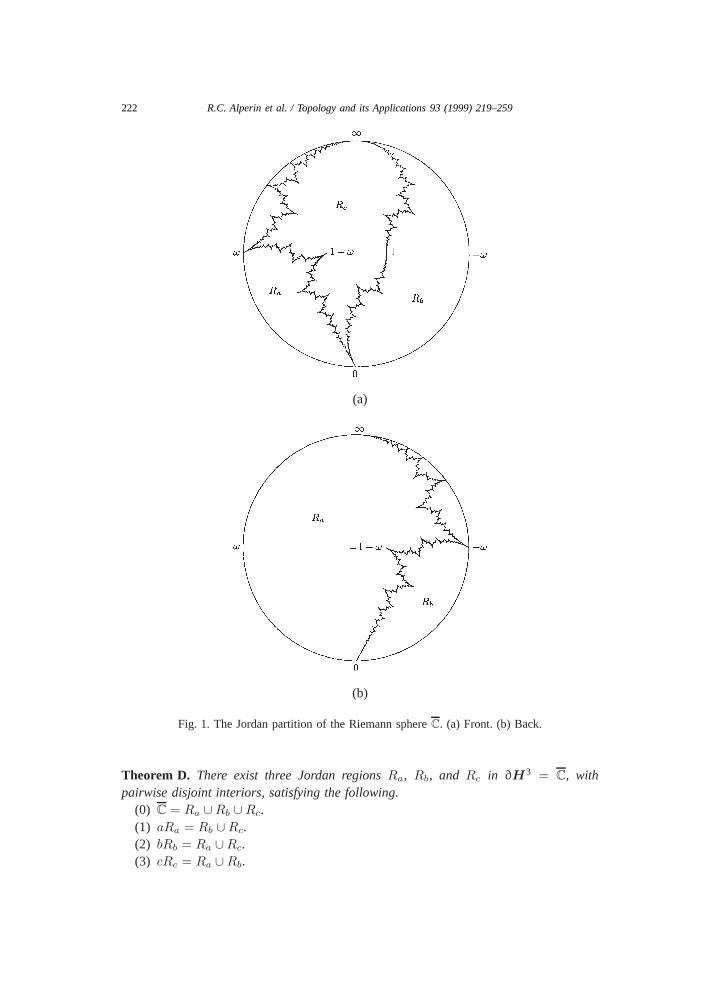
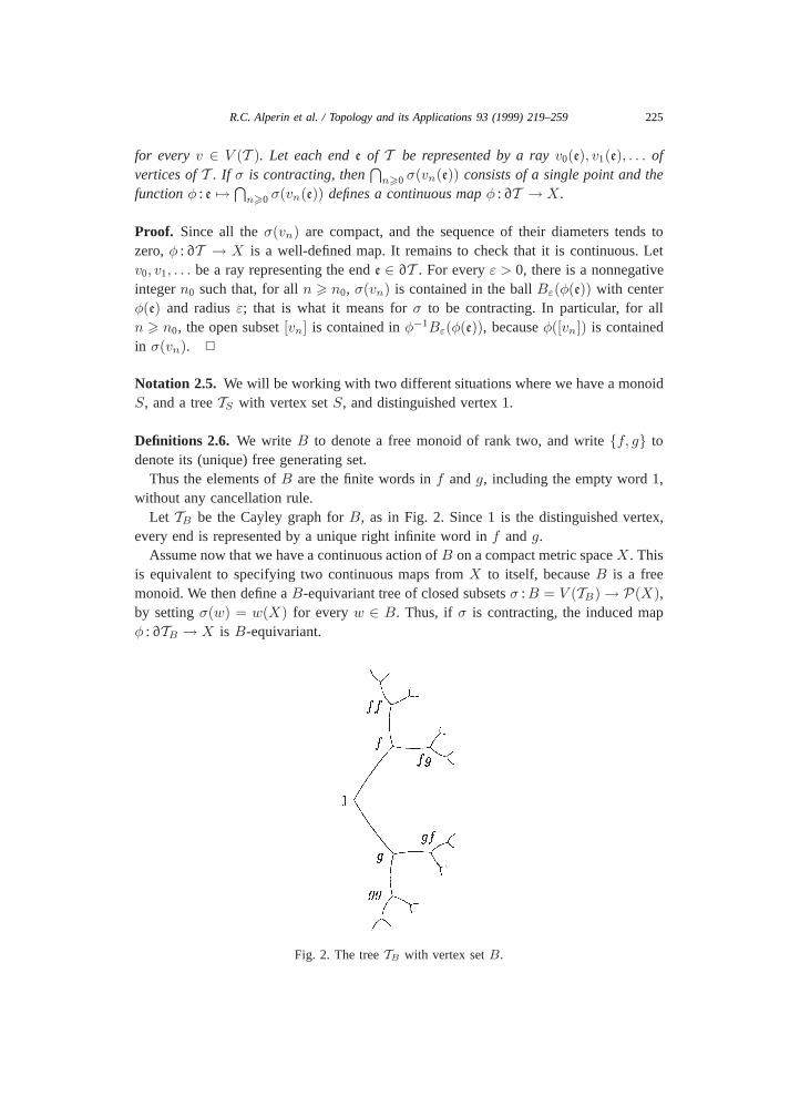
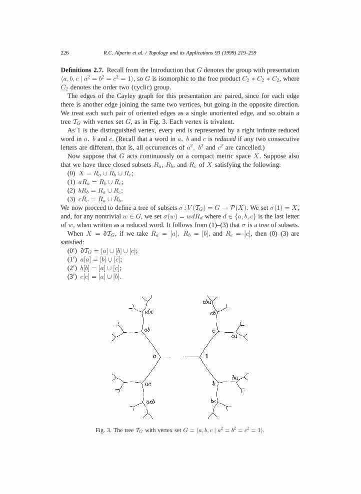
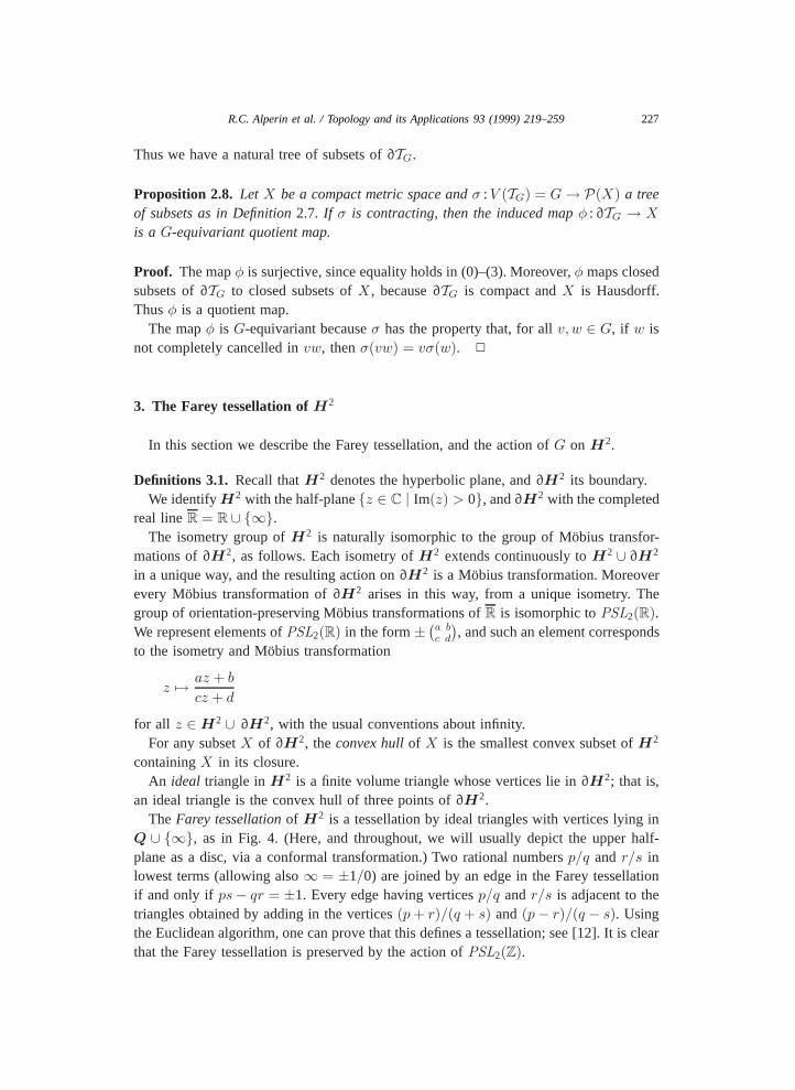
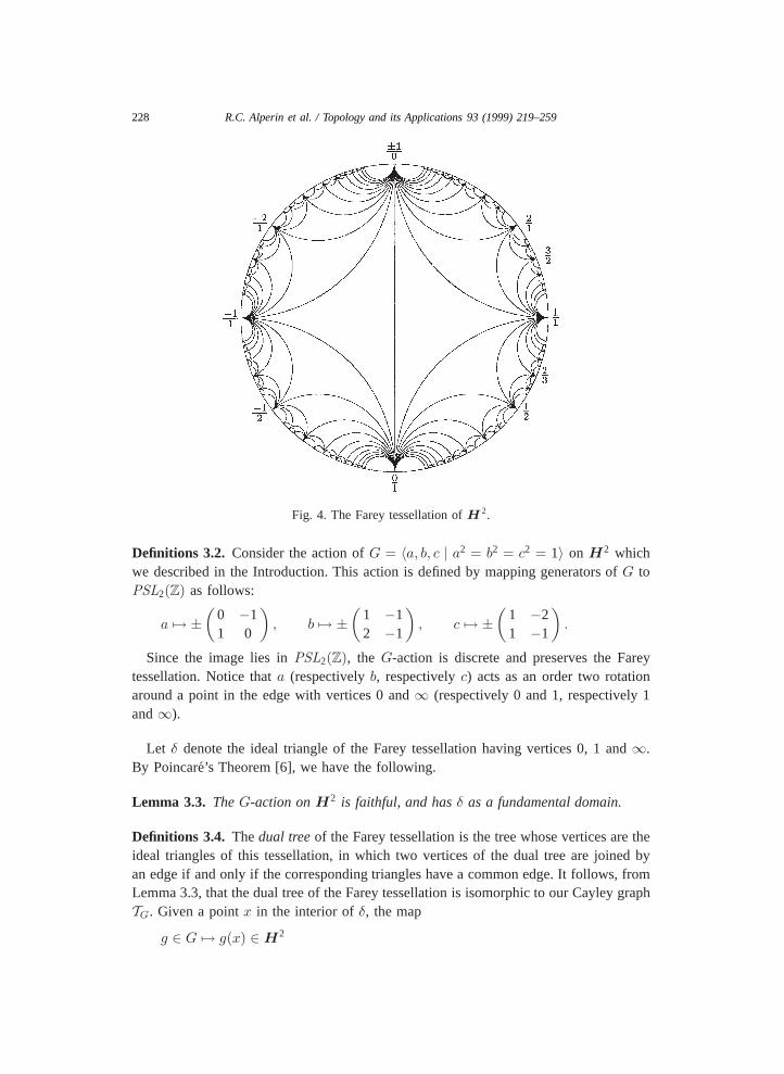
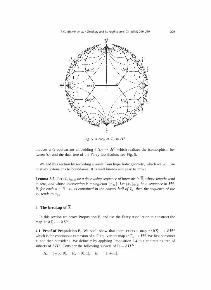
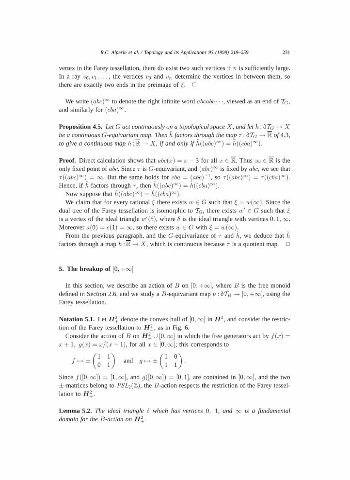
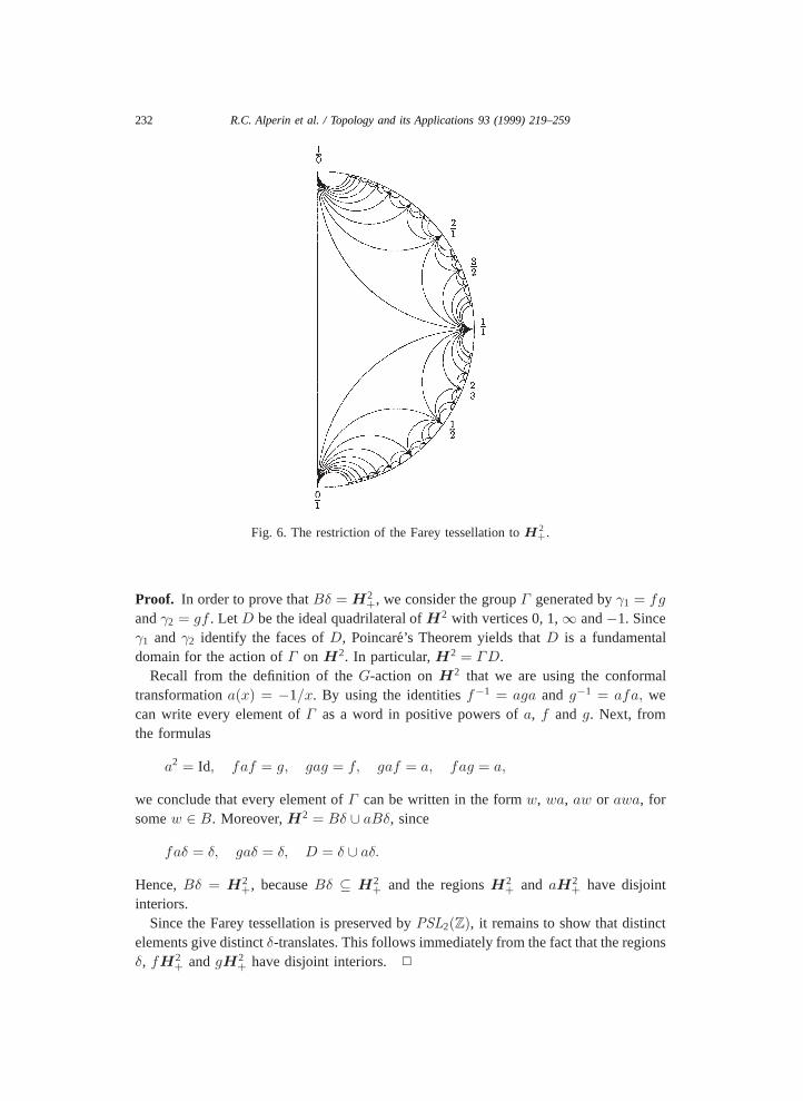
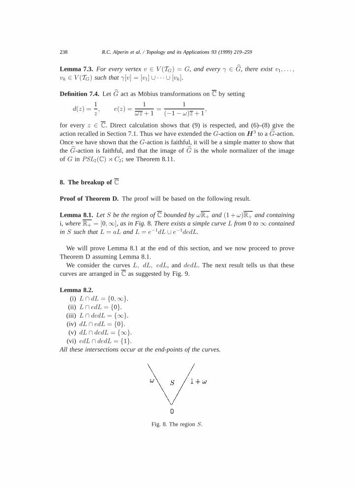
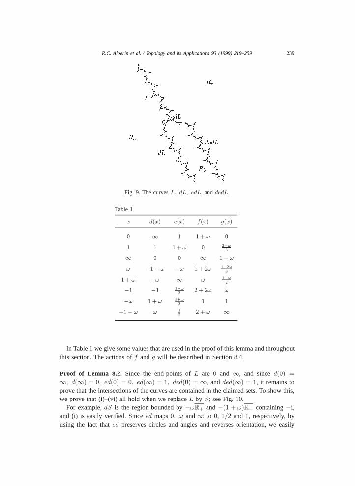
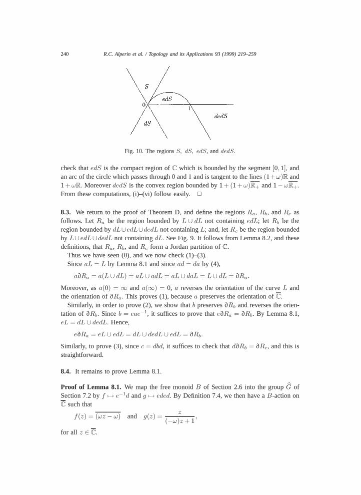
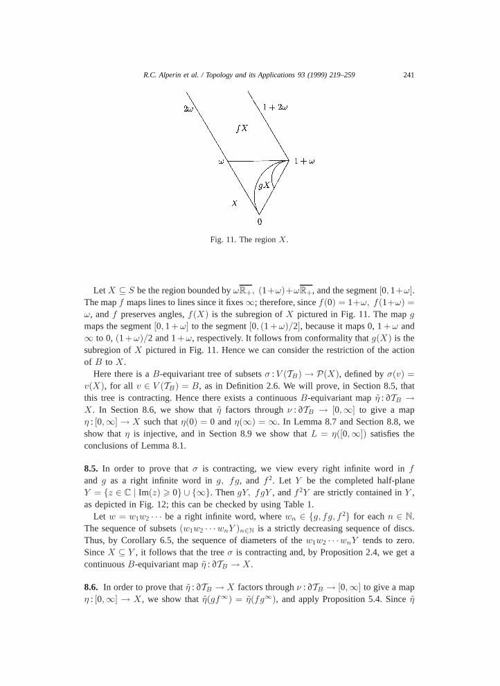
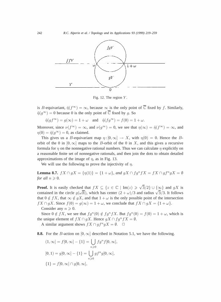
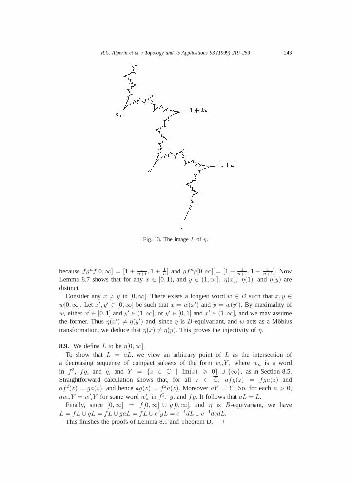
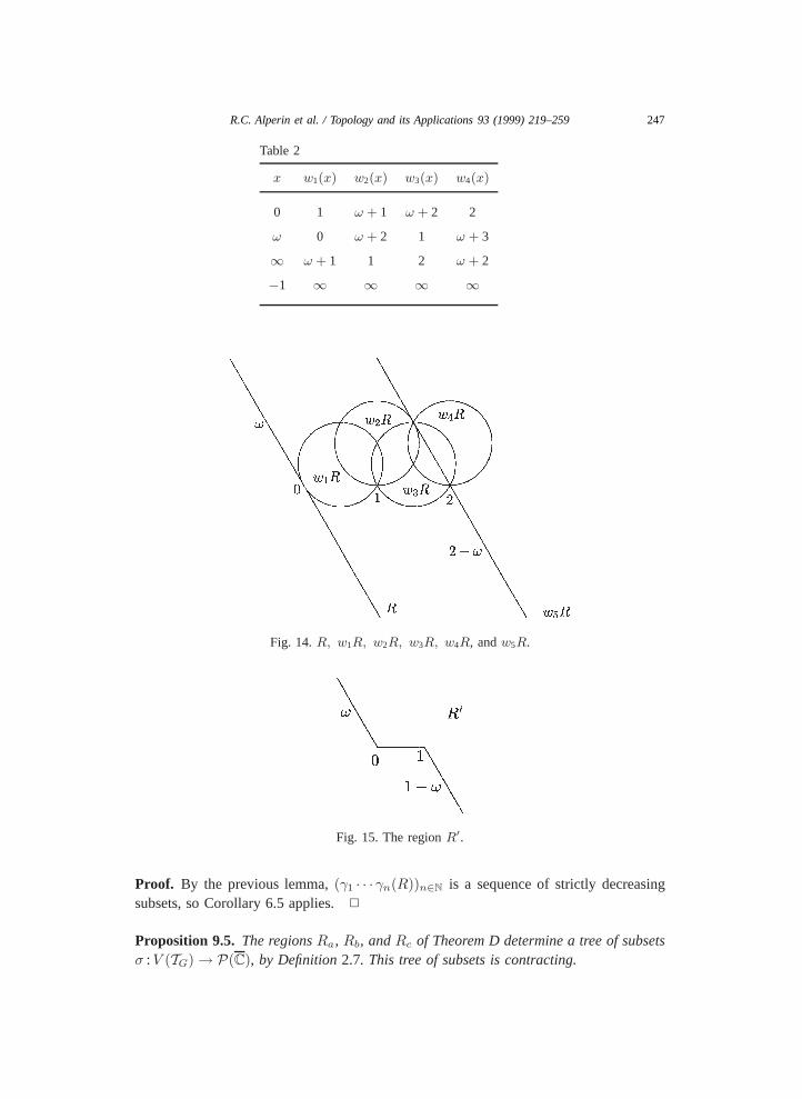
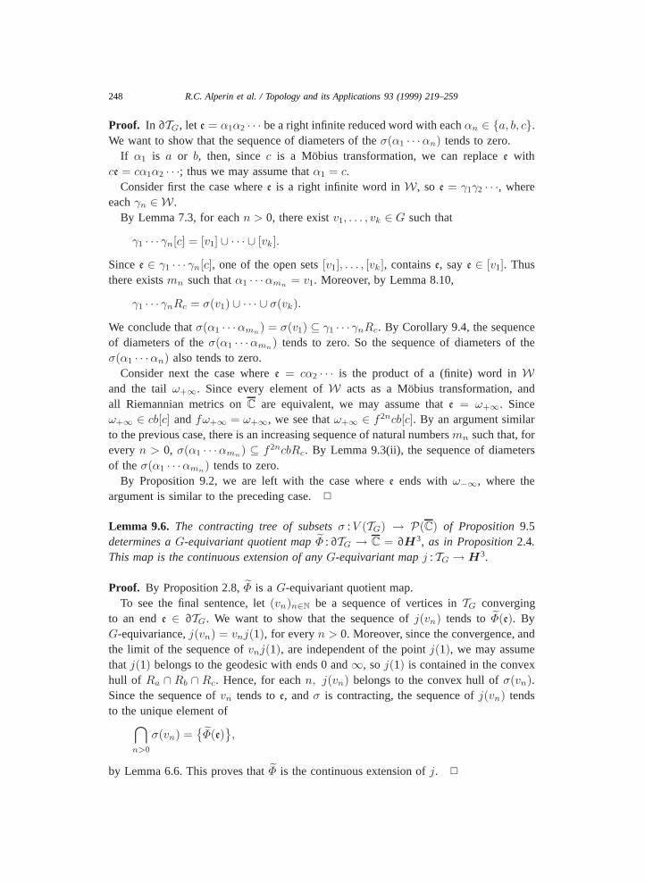

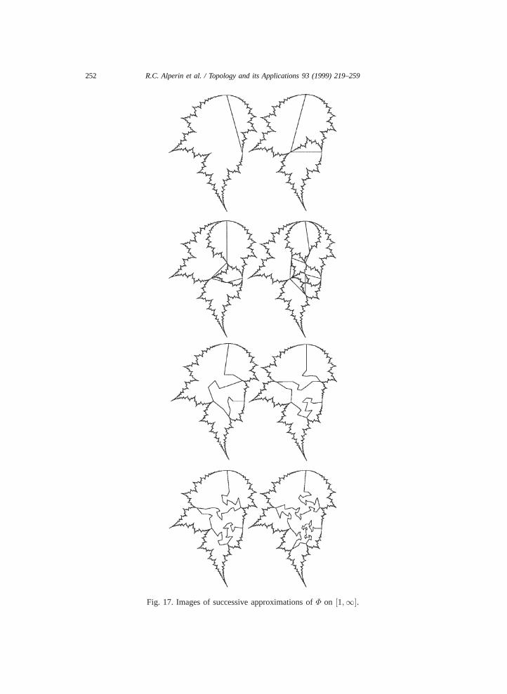
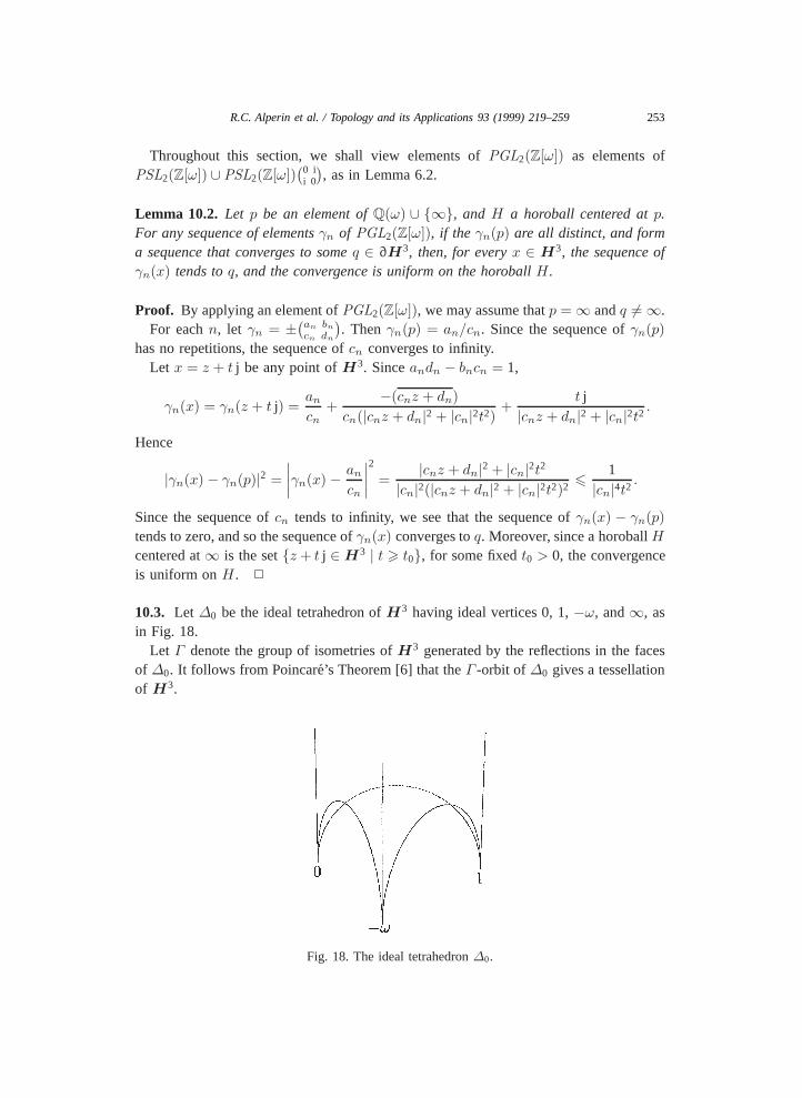


![files/Chamber/[Clarinet_Institute] Gieseking... · Created Date: 11/27/2007 9:27:20 AM](https://static.documents.pub/doc/80x56/5ae7cbb37f8b9a08778ed4fc/-clarinetinstitute-giesekingcreated-date-11272007-92720-am.jpg)


