This article was downloaded by: [Universitaets und Landesbibliothek]On: 27 August 2013, At: 07:47Publisher: Taylor & FrancisInforma Ltd Registered in England and Wales Registered Number: 1072954 Registered office: MortimerHouse, 37-41 Mortimer Street, London W1T 3JH, UK

Econometric ReviewsPublication details, including instructions for authors and subscription information:http://www.tandfonline.com/loi/lecr20

The coefficient of determination and its adjustedversion in linear regression modelsAnil K. Srivastava a , Virendra K. Srivastava a & Aman Ullah ba Department of Statistics, Lucknow University, Lucknow, Indiab Department of Economics, University of California, Riverside, CA, U.S.APublished online: 16 Feb 2011.

To cite this article: Anil K. Srivastava , Virendra K. Srivastava & Aman Ullah (1995) The coefficient ofdetermination and its adjusted version in linear regression models, Econometric Reviews, 14:2, 229-240, DOI:10.1080/07474939508800317

To link to this article: http://dx.doi.org/10.1080/07474939508800317

PLEASE SCROLL DOWN FOR ARTICLE

Taylor & Francis makes every effort to ensure the accuracy of all the information (the “Content”)contained in the publications on our platform. However, Taylor & Francis, our agents, and our licensorsmake no representations or warranties whatsoever as to the accuracy, completeness, or suitabilityfor any purpose of the Content. Any opinions and views expressed in this publication are the opinionsand views of the authors, and are not the views of or endorsed by Taylor & Francis. The accuracy ofthe Content should not be relied upon and should be independently verified with primary sources ofinformation. Taylor and Francis shall not be liable for any losses, actions, claims, proceedings, demands,costs, expenses, damages, and other liabilities whatsoever or howsoever caused arising directly orindirectly in connection with, in relation to or arising out of the use of the Content.

This article may be used for research, teaching, and private study purposes. Any substantial orsystematic reproduction, redistribution, reselling, loan, sub-licensing, systematic supply, or distribution inany form to anyone is expressly forbidden. Terms & Conditions of access and use can be found at http://www.tandfonline.com/page/terms-and-conditions

ECONOMETRIC REVIEWS, 14(2), 229-240 (1995)

THE COEFFICIENT OF DETERMINATION AND ITS ADJUSTED VERSION IN LINEAR REGRESSION MODELS

Anil K. Srivastava Virendra K. Srivastava Department of Statistics Lucknow University Lucknow, India

Aman Ullah Department of Economics

University of California Riverside, CA, U.S.A

Key Words and Phrases: regression models; quadratic forms; coefficient of determination (R2); bias; mean squared error; non-normal errors.

JEL classification: C1, C12, C13

ABSTRACT

This article presents a comparative study of the efficiency properties of the coefficient of determination and its adjusted version in linear regression models when disturbances are not necessarily normal.

1. INTRODUCTION

In applied work, the coefficient of determination (a2) is most commonly

used to judge the fit of a linear regression model. But an important and well

known limitation of R2 is that its value rises and approaches one as more

and more explanatory variables, be they relevant or not, are included in the

model. This is obviously an undesirable feature. In a bid to circumvent this

problem, a correction for the degrees of freedom is applied to R2 leading to

R i which is popularly known as adjusted R'.

Copyright 1995 by Marcel Dekker, Inc.

Dow

nloa

ded

by [

Uni

vers

itaet

s un

d L

ande

sbib

lioth

ek]

at 0

7:47

27

Aug

ust 2

013

230 SRIVASTAVA, SRIVASTAVA, AND ULLAH

In an interesting paper, observing that R2 and Rz have identical prob-

ability limits so that R2 and Ri can be regarded as consistent estimators

of certain population analogue, Cramer (1 987) obtained their exact means

and variances assuming normality of disturbances. A general finding which

emerges from his analysis is that Ri has relatively a smaller bias but has

a larger variance as compared to R2. However, he did not compare the

mean squared error (MSE) of R2 and Ri. In a recent paper, Ohtani and

Hasegawa (1993) obtained the exact moments of R2 and Ri when some re-

gressors in the regression model are proxy variables and the distrubances

follow a multivariate-t distribution. Since the exact results were extremely

complicated and no analytical comparison of the bias and MSE seemed pos-

sible, Ohtani and Hasegawa resorted to numerical calculations for specified

values of the parameters. Their results show that if the proxy variable is an

important variable, Ri can be more unreliable in small samples compared to

R2 from both the bias and MSE comparisons.

It is now well known that R2 can be expressed as a ratio of quadratic

forms. In view of this, the r- th order moments of R2, under normality, can

easily be written from the moments of the ratio of quadratic forms given

in Magnus (1986), Smith (1989, 1993) and Ullah (1990). Further, since R2

is scale invariant, these results will continue to be exact for any spherically

symmetric error density, the special cases of which are normal and multivari-

ate t densities. Furthermore, the exact moments of R2 can also be written

under the Edgeworth type density of disturbances from the results of, for ex-

ample, Peters (1989). However, these results, as in the case of Cramer (1987)

and Ohtani and Hasegawa (1993), will be extremely complicated functions of

unknown parameters and they will not be able to provide any meaningful an-

alytical comparisons of bias and MSE. One will have to resort to evaluating

the complicated expressions for specified values of parameters.

In this paper, we study the bias and MSE properties of R2 and R: for

the general set up, that is without imposing restrictions on the form of the

Dow

nloa

ded

by [

Uni

vers

itaet

s un

d L

ande

sbib

lioth

ek]

at 0

7:47

27

Aug

ust 2

013

COEFFICIENT OF DETERMINATION 23 1

distribution of disturbances. On the basis of the relationship between R2

and Rz, it has been shown that the exact bias of Rz will always be smaller

than that of R2. This result is straightforward and it does not need deriva-

tion of the exact means under specific distributions and their evaluations for

specified parameters. We also provide conditions under which R: dominates

R2 in the sense of having lower MSE. To analyse the analytical properties of

R2 and R: further we also develop the large-sample asymptotic expansions

of the bias and MSE of R2 and R: when the disturbances are i.i.d and non-

normal. These expansions provide simple expressions, and they give neat

analytical conditions of dominance of R: over R2. Such analytical results, as

far as the authors are aware, are not available in the literature. The perfor-

mance of the large-sample expansions is also examined. In an earlier paper,

Ullah and Srivastava (1994) gave the small-a approximate bias of R2 and

R:. However, neither the MSE expressions were given nor the dominance

condition obtained. Further, in general, the small-a approximations do not

povide results for the large-sample approximations. We also note that while

the i.i.d univariate t distribution is a special case of i.i.d non-normal distri-

butions considered for our approximate results, the multivariate- t considered

in Ohtani and Hasegawa (1993) is not a special case. In view of this and the

fact that Ohtani and Hasegawa (1993) c~nsider proxy variables, our analyti-

cal MSE results can not be directly comparable with their numerical results.

Also, they do not obtain any analytical dominance condition, which is the

main focus of this paper.

The plan of the paper is as follows. In the next section, we introduce

the model and estimators and their properties. Then the results presented

in this section are derived in the Appendix.

2. THE ESTIMATORS AND THEIR PROPERTIES

Let us postulate the following linear regression model

Dow

nloa

ded

by [

Uni

vers

itaet

s un

d L

ande

sbib

lioth

ek]

at 0

7:47

27

Aug

ust 2

013

232 SRIVASTAVA, SRIVASTAVA, AND ULLAH

where y is a n x 1 vector of n observations on the study variable, e is a n x 1

vector with all its elements unity, X is a n x p full column rank matrix of n

observations on p explanatory variables, cr and P are the associated regression

parameters and u is a n x 1 vector of disturbances with mean vector 0 and

variance-covariance matrix a2 I,, a2 being an unknown quantity.

Writing A = I, - n-lee', the goodness-of-fit measure R2 ( 0 5 R2 5 1 )

is given by

R2 = y l ~ ~ ( ~ l ~ ~ ) - l ~ t ~ y

Y' AY while the adjusted version of R2 is obtained by applying correction for the

loss of degrees of freedom in R2 and is given by

Cramer (1987; Sec. 3) has pointed out that R: has the same probability

limit as R2 provided all the explanatory variables in the model are asymptoti-

cally cooperative in the sense that the limiting form of matrix n- ' (X'AX) as

n + m is finite and non-singular. Consequently, both R2 and R: can be re-

garded as consistent estimators of their population counterpart @ (0 < @ < 1 )

defined by

which is a sort of 'population' measure of goodness-of-fit.

Let us, therefore, study the efficiency properties of R2 and R: for the

general setup, that is without imposing any restrictions on the distribution

of disturbances. For this purpose, we note from (3) that

Thus, E(Ri- R2) 5 0 which implies that E R ~ 5 ER2 or ER: -9 5 ER2-9.

That is the bias of R: is always smaller than that of R2,

Dow

nloa

ded

by [

Uni

vers

itaet

s un

d L

ande

sbib

lioth

ek]

at 0

7:47

27

Aug

ust 2

013

COEFFICIENT OF DETERMINATION 233

where B(R2) = ER2 - 0 is the bias of R2.

We note that the result in ( 6 ) is the exact result for any distribution

of distrubances. In the special cases of normality in Cramer (1987) and

multivariate-t in Ohtani and Hasegawa (1993) , the result in ( 6 ) is reflected

in their numerical calculations.

Next, as pointed out by Cramer (1987) , from (3)

That is, the exact variance of Rz is always larger than the variance of R2.

Now we turn to the MSE of R2 and R:. For this, we note from (3) that

Hence, squaring ( 8 ) and taking expectations on both sides we get

where M(R2) is the MSE of R2. It therefore follows from ( 9 ) that

provided D 2 0, that is

where we note that E(l - R2) 2 E(l - R2)2 because ( 1 - R2) 2 ( 1 - R2)2.

It is clear that the MSE comparison of Rz over R2 is not'as straightforward

as those of bias and variance, and it may be the case that in some situations

the MSE of Ri may behave well while in other situations the MSE of R2

Dow

nloa

ded

by [

Uni

vers

itaet

s un

d L

ande

sbib

lioth

ek]

at 0

7:47

27

Aug

ust 2

013

234 SRIVASTAVA, SRIVASTAVA, AND ULLAH

may perform better. This will be explored below by using large-sample

approximations.

In order to get further insight on the condition (11) and the bias and

MSE properties of R2 and R i , we assume that the elements of u are i.i.d with

first four finite moments as 0, u2, u3yl, and a4(y2 + 3) where yl and 72 are

Pearson's measures of skewness and kurtosis respectively of the distribution

of disturbances. Thus, we do not specify any form of the distribution of

disturbances. In a special case when the disturbances are normal, yl = y2 =

0.

Theorem: T h e large s a m p l e a s y m p t o t i c a p p r o x i m a t i o n s f o r t h e bias o f R2

a n d R: t o o r d e r O(n-l) are g i v e n b y

a n d t h e d i f f e rence in t h e i r respect ive m e a n squared errors , v i z . M(R2) a n d

M(R:), t o o r d e r O(n-2) i s g i v e n b y

These results are derived in the Appendix. We observe that the approx-

imate results in the above Theorem are for the normal (y2 = 0) as well as

for the non-normal disturbances (72 # 0).

From (12) and (13), it is observed that both R2 and R: are biased

estimators of 8. Also, though the bias approximations of both R2 and R i

are implicitly affected by p through the parameter 8, the bias approximation

of R i does not explicitly contain p while that of R2 does.

We also note that the bias of R2 and R: are not affected by the asym-

metry of the disturbances, though kurtosis does have its impact on the mag-

Dow

nloa

ded

by [

Uni

vers

itaet

s un

d L

ande

sbib

lioth

ek]

at 0

7:47

27

Aug

ust 2

013

COEFFICIENT OF DETERMINATION 235

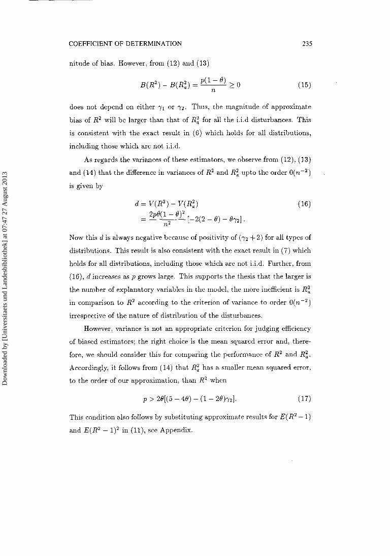
nitude of bias. However, from (12 ) and (13)

does not depend on either 71 or 72. Thus, the magnitude of approximate

bias of R2 will be larger than that of Rz for all the i.i.d disturbances. This

is consistent with the exact result in (6) which holds for all distributions,

including those which are not i.i.d.

As regards the variances of these estimators, we observe from (12), (13 )

and (14) that the difference in variances of R2 and R: upto the order O(n-2)

is given by

Now this d is always negative because of positivity of (72 + 2 ) for all types of

distributions. This result is also consistent with the exact result in (7) which

holds for all distributions, including those which are not i.i.d. Further, from

(16), d increases as p grows large. This supports the thesis that the larger is

the number of explanatory variables in the model, the more inefficient is R:

in comparison to R2 according to the criterion of variance to order O(n-2)

irrespective of the nature of distribution of the disturbances.

However, variance is not a n appropriate criterion for judging efficiency

of biased estimators; the right choice is the mean squared error and, there-

fore, we should consider this for comparing the performance of R2 and R:.

Accordingly, it follows from (14) that Rz has a smaller mean squared error,

to the order of our approximation, than R2 when

This condition also follows by substituting approximate results for E(R2 - 1)

and E(R2 - 1)2 in ( l l ) , see Appendix.

Dow

nloa

ded

by [

Uni

vers

itaet

s un

d L

ande

sbib

lioth

ek]

at 0

7:47

27

Aug

ust 2

013

236 SRIVASTAVA, SRIVASTAVA, AND ULLAH

Now if the disturbances are mesokurtic, that is, if they are normally

distributed (72 = O), the condition (17) reduces to

which holds true for all values of 6' so long as p exceeds 3; see the following

Table.

TABLE

Thus, we observe from (18) that when the distribution of disturbances

is mesokurtic (normal), R: is definitely superior to R2 as long as the number

of explanatory variables is four or more, in the sense that R: has not only

smaller bias but smaller mean squared error too. This result may hold for

three or less explanatory variables also provided 0 is small enough, with

6' 5 .2 two explanatory variables are enough.

When the distribution of disturbances departs from normality, it follows

from inequality (17) and the table given above that R: is more efficient

than R2 for all platykurtic distributions (-2 5 7 2 < 0), at least as long

as p exceeds three. This result continues to remain true for all leptokurtic

distributions (y2 > 0) also provided 0 does not fall below 0.5, i.e., the model

does not fit the data very poorly. When 6' is less than 0.5 so that the model

fits poorly, the condition (17) for superiority of R: over R2 may require

p to be somewhat larger depending upon the value of 7 2 for leptokurtic

distributions.

It is thus found that the adjusted R2(R:) is not that unreliable as it

emerges out to be from variance viewpoint alone.

Dow

nloa

ded

by [

Uni

vers

itaet

s un

d L

ande

sbib

lioth

ek]

at 0

7:47

27

Aug

ust 2

013

COEFFICIENT OF DETERMINATION 237

Now we look into the question of the limitations of the approximate

result. For this we make the following observations. It is interesting to

note that both the results B(R2) 2 B ( R ~ ) in (15) and V(R2) 5 V(Rz)

in (16), based on large-n approximations, are the same as the exact results

given in (6) and (7), respectively. Also, under the normality assumption, a

comparison of the exact bias of R2 given in the Table 1 of Cramer (1987)

with the corresponding calculations of approximate bias from (12) suggests

that the two results are quite close. For example, when p = 1 (5 = 2

in Cramer) and 0 = .9, we get the exact bias with approximate bias in

parenthesis as .036 (.034), .018 (.017), .006 (.006), .002 (.002) for n = 5,

10, 30, 100, respectively. For p = 2, 0 = .9 and the same n values, in

order, we get .057 (.054), .028 (.027), ,009 (.009), ,003 (.003). Though not

reported here, similar results were obtained for other values of 0 considered

in Cramer (1987). The same phenomenon occurred in the case of MSE

comparisons of the exact versus the approximate results. Again, when p = 1

and 0 = .9, the exact and approximate values of D = M(R2) - M(Rz)

were -.001 (-.0006), -.00018 (-.00015), .0000 (.0000) for n = 5, 10 and 30,

respectively. Note that while the approximate D is calculated by using (14),

the exact value of D is calculated by noting that we can rewrite D from (9) as

D = r[2(1- O)(r + 1)B(R2) - (2 + r ) M ( R 2 ) - r (1 -@)'I and using the results

in Table 1 of Cramer. It is thus clear that the approximate numerical results

in the normal case are very close to the corresponding exact results and

they are identical when n is thirty and above. Also, as indicated above, the

analytical comparisons of the approximate bias and variance, in the general

non-normal case, provide the same results as those based on the exact results.

Nevertheless, it remains the subject of a future study to see if the dominance

condition in (17) and (18), based on the approximate MSE, will go through

for the exact MSE case.

Dow

nloa

ded

by [

Uni

vers

itaet

s un

d L

ande

sbib

lioth

ek]

at 0

7:47

27

Aug

ust 2

013

SKIVASTAVA, SRIVASTAVA, AND ULLAH

APPENDIX

In order to derive the results given in the Theorem, we first state the

following results:

u - ~ E ( u ' B u u ' ) = ylel(In * B ) ( 2 )

u - ~ E ( u ' B u . U U ' ) = y2(In * B ) + ( t r B ) I n + 2 B ( i i )

where B is a n x n symmetric matrix with non-stochastic elements; see, e.g.,

Ullah, Srivastava and Chandra (1983, p. 398).

Now writing

w = (G - 2)

and substituting ( 1 ) in ( 2 ) , we observe that

P'X 'AXP + 2u'AXP + U ' A X ( X ' A X ) - ' X ' A U ( R 2 - 0 ) = - O

P 'X 'AXP + nu2 + ( n w + 2u1AXP) - n - l ( ~ ' e ) ~

-- - (' - O ) [2(1 - O ) U ' A X P - Onw + U ~ A X ( X ~ A X ) - ' X ~ A U nu2

+ n - ' ~ ( u ' e ) ~ ] .

Expanding the right hand side, we find

( R 2 - 0 ) = ( 1 - O ) ( f - + + 5-1) + 0 p ( n - 3 / 2 ) ( i i i )

where, denoting f - , as a term of O p ( n - T ) ,

1 f - 3 = - [2(1 - O)ulAXP - Onw]

nu2 1 6 4(1 - 0)2

f- l = z ~ ' [ ~ ~ ( ~ ' ~ ~ ) - l ~ ' ~ + -eel - n nu2 A X P P ' X A ] . u

+ (1-8)[On2w2 - 2(1 - 2O)nw . u 'AXP] . n2u4

Thus, the bias of R2 to order ~ ( n - l ) is given by

Dow

nloa

ded

by [

Uni

vers

itaet

s un

d L

ande

sbib

lioth

ek]

at 0

7:47

27

Aug

ust 2

013

COEFFICIENT OF DETERMINATION

Using (i) and (ii), it is easy to see that

which, when substituted in (iv) leads to result (12) of the paper.

For deriving the result (13), we observe from (3) and (iii) that

Thus, the bias of Ri to order O(n-l) is given by

Substituting the expectations, we obtain the result (13).

Finally, let us consider the difference in mean squared errors of R2 and

RZ, to order ~ ( n - ~ ) . Using (iii), we have

n - p - 1

- - 2p(l - q2 2 P

E (f-; +f-1 -f-i - -) +0(n-') (vii) n 2 2n

It is easy to verify that

8 (f!;) = ;(4 - 28 + 672) (viii)

Substituting it along with the expectations of f-l and f-l in (vii), we

obtain the result (14) of the paper.

Fianlly, we note that E(l - R2) = (1 - 0) - B(R2), and E(l - R2)2 =

(1 - B2 - 2(1 - 8)B(R2) + (1 - 8 ) 2 E f ~ l 1 2 upto O(n-l). Substituting these

values in (1 I ) , we can get the condition in (17).

Dow

nloa

ded

by [

Uni

vers

itaet

s un

d L

ande

sbib

lioth

ek]

at 0

7:47

27

Aug

ust 2

013

SRIVASTAVA, SRIVASTAVA, AND ULLAH

ACKNOWLEDGEMENTS

The authors are thankful to E. Maasourni and two referees for their

valuable suggestions and constructive comments. The third author gratefully

acknowledges the financial support from the Academic Senate, UCR.

REFERENCES

Cramer, J.S. (1987): Mean and Variance of R2 in Small and Moderate Sam- ples, Journal of Econometrics, 35, 253-266.

Magnus, J.R. (1986): The Exact Moments of a Ratio of Quadratic Forms in Normal Variables, Annales of Economie et de Statistique, 4, 95-109.

Ohtani, L. and H. Hasegawa (1993): On Small-Sample Properties of R2 in a Linear Regression Model with Multivariate t Errors and Proxy Variables, Econometric Theory, 9, 504-515.

Peters, T.A. (1989): The Exact Moments of OLS in Dynamic Regression Models with Non-normal Errors, Journal of Econometrics, 279-305.

Smith, M.D. (1989): On the Expectation of a Ratio of Quadratic Forms in Normal Variables, Journal of Multivariate Analysis, 31, 244-257.

Smith, M.D. (1993): Expectations of Ratios of Quadratic Forms in Nor- mal Variables: Evaluating Some Top-Order Invariant Polynomials, Aus- tralian Journal of Statistics, 271-282.

Ullah, A. (1990): Finite Sample Econometrics: A Unified Approach in R.A.L. Carter, J . Dutta and A. Ullah, eds. Contributions to Econometric The- ory and Application. Springer-Verlag, New York, 249-292.

Ullah, A. and V.K. Srivastava (1994): Moments of the Ratio of Quadratic Forms in Non-normal Variables with Econometric Examples, Journal of Econometrics, 62, 129-142.

Ullah, A., V.K. Srivastava and R. Chandra (1983): Properties of Shrinkage Estimators in Linear Regression when Disturbances are not Normal, Journal of Econometrics, 21, 389-402.

Dow

nloa

ded

by [

Uni

vers

itaet

s un

d L

ande

sbib

lioth

ek]

at 0

7:47

27

Aug

ust 2

013