The Contribution of Radiative Feedbacks to Orbitally Driven Climate Change

MICHAEL P. ERB AND ANTHONY J. BROCCOLI

Department of Environmental Sciences, Rutgers, The State University of New Jersey, New Brunswick, New Jersey

AMY C. CLEMENT

Rosenstiel School of Marine and Atmospheric Science, University of Miami, Miami, Florida

(Manuscript received 2 July 2012, in final form 5 February 2013)

ABSTRACT

Radiative feedbacks influence Earth’s climate response to orbital forcing, amplifying some aspects of the

response while damping others. To better understand this relationship, the GFDL Climate Model, version

2.1 (CM2.1), is used to perform idealized simulations in which only orbital parameters are altered while ice

sheets, atmospheric composition, and other climate forcings are prescribed at preindustrial levels. These

idealized simulations isolate the climate response and radiative feedbacks to changes in obliquity and

longitude of the perihelion alone. Analysis shows that, despite being forced only by a redistribution of

insolation with no global annual-mean component, feedbacks induce significant global-mean climate

change, resulting in mean temperature changes of 20.5K in a lowered obliquity experiment and 10.6K in

a NH winter solstice perihelion minus NH summer solstice perihelion experiment. In the obliquity ex-

periment, some global-mean temperature response may be attributable to vertical variations in the

transport of moist static energy anomalies, which can affect radiative feedbacks in remote regions by al-

tering atmospheric stability. In the precession experiment, cloud feedbacks alter the Arctic radiation

balance with possible implications for glaciation. At times when the orbital configuration favors glaciation,

reductions in cloud water content and low-cloud fraction partially counteract changes in summer insolation,

posing an additional challenge to understanding glacial inception. Additionally, several systems, such as the

Hadley circulation and monsoons, influence climate feedbacks in ways that would not be anticipated from

analysis of feedbacks in the more familiar case of anthropogenic forcing, emphasizing the complexity of

feedback responses.

1. Introduction

Paleoclimate modeling and data studies suggest that

large periodic variations in past global-mean tempera-

ture have been driven by cyclical changes in Earth’s ec-

centricity, obliquity, and longitude of the perihelion. By

dictating the earth’s orbital geometry, these three cycles

alter the seasonal and latitudinal distribution of inso-

lation, which (amplified by internal climate system feed-

backs) can result in global-mean climate change. The idea

that orbital cycles are responsible for glacial–interglacial

cycles and other Quaternary variations was championed

by Milankovitch (1941) and has since been expanded in

work by Hays et al. (1976) and numerous others in more

recent times (e.g., Imbrie et al. 1993; Raymo and

Nisancioglu 2003). For glacial–interglacial cycles, low

obliquity (axial tilt) and Northern Hemisphere (NH)

winter solstice perihelion encourage ice sheet expansion

by reducing NH summer insolation. This orbital theory

suggests that by allowing ice to survive through the less

intense melt season, additional ice may accumulate dur-

ing the winter, cooling the earth through a positive ice–

albedo feedback.

Orbital signals in the proxy record have been well

documented (e.g., Petit et al. 1999; Jouzel et al. 2007),

but uncertainties remain concerning the exact climatic

effects of orbital forcing. Hypotheses have been pro-

posed to answer unresolved questions such as why climate

variations dominantly occur with 100-kyr periodicity in

the late Pleistocene (Imbrie et al. 1993;Huybers 2006) and

why 40kyr is the dominant period in the early Pleistocene

(Raymo and Nisancioglu 2003; Huybers 2006; Huybers

and Tziperman 2008). Because global annual-mean

Corresponding author address: Michael P. Erb, Department of

Environmental Sciences, Rutgers, The State University of New

Jersey, 14 College Farm Road, New Brunswick, NJ 08901.

E-mail: mperb@envsci.rutgers.edu

15 AUGUST 2013 ERB ET AL . 5897

DOI: 10.1175/JCLI-D-12-00419.1

� 2013 American Meteorological Society

radiative forcing caused by orbital cycles is exceedingly

small, substantial climate feedbacks are necessary to

explain global-mean climate shifts.

General circulation models provide a useful way to

investigate the role of feedbacks in orbitally forced cli-

mate change. While much focus in modeling has been

placed on specific time periods such as the last glacial

maximum, last interglacial, and the mid-Holocene, at-

tribution of the influence of orbital signals in such simu-

lations is complicated by competing effects from changes

in ice sheets and atmospheric composition. Idealized

simulations in which only the orbital configuration is

changed can provide a clearer picture of the feedback

response.

Several studies using idealized simulations have al-

ready been completed, with early work being done by

Phillipps and Held (1994), who investigated the climate

response under various orbital configurations. More re-

cently, Jackson and Broccoli (2003) ran an atmosphere–

slab oceanmodel forced with only the accelerated orbital

forcing of the past 165 kyr and found that low obliquity

and late NH spring aphelion led to enhanced snow ac-

cumulation at times mostly consistent with the proxy re-

cord, largely influenced by storm activity and feedbacks

involving sea ice. Further analysis highlighted the im-

portance of atmospheric dynamics such as the northern

annular mode (Hall et al. 2005). Other idealized orbital

forcing studies have focused on the roles of vegetation

and sea ice (Tuenter et al. 2005a,b), the effect of pre-

cession at the last interglacial (Khodri et al. 2005), the

response of the tropical climate to orbital forcing

(Clement et al. 2004; Lee and Poulsen 2005; Timmermann

et al. 2007), the response of monsoons to orbital forcing

(Wyrwoll et al. 2007), and feedbacks in response to changes

in obliquity (Lee and Poulsen 2008; Mantsis et al. 2011).

In this study, a fully coupled atmosphere–ocean gen-

eral circulation model (AOGCM) is employed to fur-

ther explore the role of feedbacks in orbitally forced

climate simulations.While there have been other studies

that look at the climate response to orbital cycles, little

focus has been placed on the role of radiative feedbacks,

particularly with a fully coupled AOGCM. In addition,

a novel aspect of this research is the use of the kernel

method of feedback analysis, which has rarely been ap-

plied to paleoclimate simulations. Another novel aspect

of this research is the idealized experimental design, in

which the climate response to changes in obliquity and

longitude of the perihelion may be isolated and explored.

To better understand the feedback response, feedbacks

computed in these orbital experiments are also compared

with feedbacks from a doubled CO2 experiment. Pre-

vious studies have suggested that feedbacks operate

similarly in simulations driven by changes in different

forcing agents (e.g., CO2, solar irradiance, and organic

carbon), although the feedbacks do show some sensi-

tivity to the latitude and altitude of the imposed forcing

(Yoshimori and Broccoli 2008). The comparison of feed-

backs under orbital and anthropogenic forcing in the

present paper provides a test of this idea and will allow

us to identify which aspects of feedback remain con-

sistent under different forcings, and which are sensitive

to the type and distribution of forcing.

The design of the orbital forcing experiments is out-

lined in section 2. Section 3 explores the temperature

response in these orbital experiments. The roles of feed-

backs in producing the modeled climate change are

discussed in section 4, and section 5 compares feed-

backs under orbital forcings to those under anthropo-

genic forcing. Section 6 considers the potential effect of

cloud feedbacks on large-scale NH ice sheet growth,

and the paper’s conclusions are stated in section 7.

2. Experimental design

The AOGCM used for this study is the Geophysical

Fluid Dynamics Laboratory (GFDL) Climate Model,

version 2.1 (CM2.1), which has atmosphere, ocean, land,

and sea ice components coupled without flux adjust-

ments. Atmospheric resolution is 28 latitude by 2.58longitude with 24 vertical levels, and ocean resolution

is 18 by 18, becoming finer in the tropics to a meridio-

nal resolution of 1/38 with 50 vertical levels (Delworth

et al. 2006). Reichler and Kim (2008) compared sim-

ulations of preindustrial climate and found that CM2.1

performed the best among the models from phase 3

of the Coupled Modeling Intercomparison Project

(CMIP3).

To explore feedback mechanisms under obliquity-

and precession-only forcing, four idealized equilibrium

simulations have been conducted (Table 1). For obliq-

uity, two simulations set obliquity to the low (22.0798)and high (24.4808) extremes of the past 600 kyr with all

other variables, such as ice sheet extent and atmospheric

TABLE 1. Orbital values for obliquity and precession simula-

tions. Obliquity simulations (Hi and Lo) represent the high and low

obliquity of the past 600 kyr (Berger and Loutre 1991). Precession

simulations (WS and SS) represent opposite times on the precession

cycle, with increased eccentricity to amplify the signal. Numbers in

italics are preindustrial values.

Simulation

Name Eccentricity

Lon of

perihelion (8) Obliquity (8)

Lo 0.01671 102.932 22.079

Hi 0.01671 102.932 24.480

WS 0.0493 90 23.439

SS 0.0493 270 23.439

5898 JOURNAL OF CL IMATE VOLUME 26

composition, prescribed at preindustrial levels. To iso-

late precession, two simulations set perihelion to theNH

winter solstice (WS) and NH summer solstice (SS) with

all other variables prescribed to preindustrial levels ex-

cept eccentricity, which is increased to 0.0493, the maxi-

mum eccentricity of the past 600kyr (Berger and Loutre

1991). Because the effects of precession on insolation

scale with eccentricity, this value of eccentricity has

been chosen to raise the signal-to-noise ratio in the

precession results. A CMIP3 (Meehl et al. 2007) dou-

bled CO2 simulation, in which CO2 is increased from

preindustrial levels at 1% yr21 until doubling and sta-

bilized at that level thereafter (Stouffer et al. 2006), is

compared with a preindustrial control run. This dou-

bled CO2 experiment is used as the basis for comparing

feedbacks under orbital forcing with those estimated

from anthropogenic forcing. Because CM2.1 lacks dy-

namic ice sheets, dynamic vegetation, and a carbon cycle,

the analysis in this paper focuses on the fast radiative

feedbacks in the climate system (i.e., surface albedo,

water vapor, lapse rate, and clouds).

In the precession results, a calendar adjustment has

been made. Because of the elliptical shape of Earth’s

orbit, changes in longitude of the perihelion alter the

lengths of seasons according to Kepler’s second law.

When comparing precession results on a standard fixed-

day calendar, this causes dates to become offset from

each other, making comparison between simulations

problematic (Joussaume and Braconnot 1997). As a

remedy for this problem, precession results have been

converted to a common fixed-angular calendar where

each ‘‘month’’ corresponds to a 308 arc of orbit. The

conversion was made using the method outlined in

Pollard and Reusch (2002), which is one of several

proposed methods (Timm et al. 2008; Chen et al. 2010).

All of the orbital forcing simulations were run for

600 years, and the results presented in this paper use

the mean of years 501–600. The precession simulations

were run on a slightly updated version of CM2.1, which

implements some bug fixes and has a slightly different

value for snow albedo as well as some other minor

changes, but these adjustments do not appear to affect

the results. For analysis purposes, results of the orbital

forcing simulations are presented as low minus high

obliquity (the Lo–Hi experiment) and NH winter sol-

stice perihelion minus NH summer solstice perihelion

(theWS–SS experiment). This convention is undertaken

so both experiments reduce the NH summer insolation,

which is conducive to NH glaciation.

The Lo–Hi experiment discussed in this paper has also

been analyzed in Mantsis et al. (2011), which uses two

different methods to investigate feedbacks in response

to obliquity changes. The present paper expands upon

the work of Mantsis et al. (2011) by exploring feedbacks

computed with the kernel method in greater depth, with

a focus on the physical mechanisms that lead to the

feedback responses. The climate response and feed-

backs in theWS–SS experiment have not been previously

explored.

3. Insolation change and temperature response

The Lo–Hi experiment is defined by a decrease in

Earth’s axial tilt from 24.4808 to 22.0798. In an annual-

mean sense, this increases top-of-atmosphere (TOA) solar

radiation in the tropics by several watts per square meter

and decreases it at higher latitudes by up to ;15Wm22,

increasing the equator-to-pole insolation gradient (Fig. 1a).

Seasonally, the amplitude of the extratropical inso-

lation cycle is reduced in both hemispheres—winter

insolation increases by over 15Wm22 and summer

insolation decreases by up to;50Wm22. In comparison,

the WS–SS experiment consists of changing Earth’s

perihelion from NH summer solstice to NH winter sol-

stice, resulting in increased insolation during the half

year centered on NH winter solstice and decreased in-

solation for the rest of the year, with monthly insolation

differences as large as;100Wm22 (Fig. 1b). TheWS–

SS insolation anomalies reach their peak in mid- and

high-latitude summer when the magnitude of insolation

FIG. 1. Seasonal changes in zonal-mean insolation (Wm22) for the (a) Lo–Hi and (b) WS–SS experiments

as a function of latitude.

15 AUGUST 2013 ERB ET AL . 5899

is largest and result in a weakening of the NH but a

strengthening of the Southern Hemisphere (SH) annual

insolation cycle.

Responding to these changes, the seasonal- and annual-

mean surface air temperature changes DT are shown for

both experiments in Fig. 2. TheLo–Hi experiment exhibits

a slightly positive DT throughout most of the tropics, av-

eraging10.1K over the tropics, with decreases in DT over

themid- and high latitudes becoming greater inmagnitude

toward the poles. In the midlatitudes, winter DT is mostly

negative despite positive insolation changes during that

season. This is because of the large heat capacity of the

upper ocean, which acts as an integrator of forcing. On

the whole, the equator-to-pole temperature gradient is

increased. Other features of the temperature response

are discussed in Mantsis et al. (2011). Importantly, neg-

ative annual-mean DT extends equatorward of negative

annual-mean insolation change, suggesting that feed-

backs can overwhelm the direct effects of local inso-

lation forcing.

In the WS–SS experiment, DT exhibits much more

seasonal variation, with most latitudes experiencing

negative DT from approximately June to October and

positiveDT through the rest of the year, which is delayed

from the insolation changes by as much as several months

because of the thermal inertia of the climate system. In

Antarctica, which is more thermally isolated by virtue of

the Antarctic Circumpolar Current, DT remains positive

through almost all of the year. Spatially, annual-mean

DT is especially positive over the North African and

Indian Ocean monsoon regions, with negative DTmostly

confined to midlatitude continents. The reasons for these

changes are explored in the following section.

In both the Lo–Hi and WS–SS experiments, global

annual-mean insolation change is zero. A more accu-

rate measure of the change in insolation felt by the

climate system is radiative forcing, which is defined by

Ramaswamy et al. (2001) as ‘‘the change in net (down

minus up) irradiance (solar plus long-wave; inWm22) at

the tropopause after allowing for stratospheric tempera-

tures to readjust to radiative equilibrium, but with surface

and tropospheric temperatures and state held fixed at the

unperturbed values.’’ In the present paper, radiative

forcing does not include longwave radiation, and strato-

spheric temperatures are not allowed to adjust. Positive

values of radiative forcing represent a heating of the cli-

mate system. Despite the absence of a net change in

global annual-mean insolation, mean radiative forcing

is 10.10Wm22 for Lo–Hi and 20.11Wm22 for WS–SS

because of the spatial and temporal covariance of in-

solation anomalies and albedo. Although the radiative

forcing is small, global-mean DT is 20.5K for Lo–Hi and

10.6K for WS–SS. This disproportionate DT response

(which is opposite to the sign of the radiative forcing in

both cases) indicates the crucial role of radiative feedbacks

in determining climate response to orbital forcing.

FIG. 2. Change in (a),(b) zonal-mean surface air temperature (K) and (c),(d) annual-mean surface air temperature

(K) for the (left) Lo–Hi and (right) WS–SS experiments.

5900 JOURNAL OF CL IMATE VOLUME 26

4. Radiative feedbacks

The ‘‘fast’’ radiative feedbacks, which are the focus

of this research, involve changes in Earth’s surface al-

bedo as, atmospheric water vapor q, vertical tempera-

ture lapse rate G, and cloud optical properties c. These

four radiative feedbacks, plus the blackbody sensitivity

dF/dT, equal the total climate sensitivity dF/dT (which

is the change in radiative forcing per unit tempera-

ture change) in CM2.1, as expressed in the following

equation:

dF

dT5

dF

dT1

dF

das

das

dT1

dF

dq

dq

dT1

dF

dG

dG

dT1

dF

dc

dc

dT.

In the absence of vegetation and geological changes,

changes in surface albedo result from variations in sea

ice and continental snow cover, which tend to enhance

climate perturbations through melt or expansion. Water

vapor is an effective greenhouse gas, so its concentration

and distribution influence the atmosphere’s ability to

affect longwave (LW) radiation and, to a smaller extent,

shortwave (SW) radiation. A change in the lapse rate

(the rate at which temperature decreases with height)

affects the loss of LW radiation to space by affecting the

emitting temperature of the upper troposphere, which

emits to space more readily than the surface. Clouds

affect the radiation balance through the absorption

and scattering of SW radiation and the absorption and

emission of LW radiation in the atmosphere, so changes

in the amount, distribution, and water content of clouds

may amplify or diminish climate perturbations.

To isolate and quantify these feedbacks, the kernel

method outlined in Soden and Held (2006) and Soden

et al. (2008) is employed. This method uses a set of ra-

diative ‘‘kernels,’’ computed using a stand-alone radia-

tion code to quantify the net changes in TOA radiation

that result from unit changes in surface albedo, water

vapor, and lapse rate at each grid point and time of year.

The cloud feedback cannot be calculated explicitly with

this method because of strong nonlinearities in the cloud

feedback, but is instead calculated by adjusting the change

in cloud radiative forcing to account for the influence

of clouds in masking noncloud feedbacks (i.e., temper-

ature, water vapor, and surface albedo; Soden et al. 2004,

2008). The kernel method is convenient because it can

differentiate the effects of concurrent radiative feed-

backswithout the need to rerunmodel code, which can be

computationally expensive. In interpreting the following

results it should be noted that the results are here ex-

pressed as the effect of feedbacks on net TOA radiation

DRnet (Wm22), rather than as feedbacks (Wm22K21).

Doing so avoids dividing by the small values of global-

mean DT in the orbital experiments. Positive values of

DRnet indicate increased net downward radiation. In the

following subsections the role of each feedback under

orbital forcing is examined. A further analysis of some of

the mechanisms at work will follow in section 5.

a. Surface albedo feedback

The DRnet from the surface albedo feedback is shown

in Figs. 3a and 3b. In the Lo–Hi experiment, the sea ice

fraction increases in the Arctic Ocean, Greenland Sea,

Barents Sea, and Bering Sea, and snow cover increases

across much of the NH high-latitude continents, in-

creasing reflection of SW radiation primarily in the NH

summer when insolation values are high. SH changes

are characterized by increases in sea ice in much of the

Southern Ocean, but snow expansion is limited by a lack

of SH midlatitude continental areas and by the thermal

isolation of Antarctica, which sustains snow cover year-

round, causing SH changes to be less extensive than NH

ones. Global-mean DRnet for each feedback is given in

Table 2. The global-mean DRnet from the surface albedo

feedback in the Lo–Hi experiment is 20.27Wm22, in-

dicating a cooling effect.

In the WS–SS experiment, snow and sea ice changes

occur in largely the same regions as the Lo–Hi experi-

ment, but present a more seasonally varying response

because of the more seasonal nature of the forcing. In

the NH, snow cover retreats more during a warmer NH

spring and Arctic sea ice retreats less during a cooler

NH summer. Aided by the large size of NH midlatitude

continents, snow retreat has a larger total effect on al-

bedo than sea ice increase, so the total effect of these

two competing NH changes is a warming. In the SH,

Southern Ocean sea ice retreats farther than normal

during the warmer SH summer. However, because of

the limited area of SH midlatitude continents, SH snow

cover anomalies during SH spring are small despite cooler

temperatures. This imbalance in the land–sea distribution

allows sea ice reductions to dominate the SH albedo

response, leading to a warming effect. Global-mean DRnet

from the surface albedo feedback is 10.31Wm22 in the

WS–SS experiment, emphasizing the importance of

seasonality and surface type in determining feedback

responses.

b. Water vapor feedback

The DRnet from the water vapor feedback is given in

Figs. 3c and 3d and is characterized by both latitudinal

and seasonal variations for Lo–Hi and mostly seasonal

variations forWS–SS, generally having a warming effect

where DT is positive and a cooling effect where DT is

negative. To see what effect circulation changes have on

this feedback, the water vapor response is separated into

two components (Fig. 4): a thermodynamic component

15 AUGUST 2013 ERB ET AL . 5901

FIG. 3. Effect of feedbacks on zonal-mean DRnet (Wm22) caused by (a),(b) surface albedo, (c),(d) water vapor,

(e),(f) lapse rate, (g),(h) clouds, and (i),(j) the sum of all four for the Lo–Hi and WS–SS experiments, respectively.

Positive values represent increased net downward radiation. Global-mean values (Wm22) are given in the bottom

right of each panel.

5902 JOURNAL OF CL IMATE VOLUME 26

that corresponds to the change in specific humidity

that would result from DT according to the Clausius–

Clapeyron relation with a fixed RH and a dynamic

component resulting from changes in atmospheric eddies

and circulation patterns.

In the Lo–Hi experiment, thermodynamic changes

are characterized by increased water vapor in the tropics,

where DT is positive, and decreased water vapor else-

where, where DT is negative. Dynamic changes show

an additional increase in tropical water vapor associated

with an enhanced annual-mean Hadley circulation, with

enhanced dry zones in regions of subtropical descent.

Enhancement of the annual-mean Hadley circulation is

consistent with the increased equator-to-pole insolation

and temperature gradients, as previously found by Otto-

Bliesner and Clement (2004) and Rind and Perlwitz

(2004).

In the WS–SS experiment, thermodynamic changes

dominate at higher latitudes, but dynamic changes are

equally large in the tropics. These dynamic changes are

primarily associated with changes in monsoons. Pre-

cipitation differences in theWS–SS experiment (Table 3)

reveal diminished NH rainy seasons in North America,

northern Africa, and Asia and enhanced SH rainy sea-

sons in South America, southern Africa, and Australia.

Changes in monsoon intensity affect the amount of water

vapor transported into continental regions, with weakened

NH monsoons transporting less water vapor into NH

continents and strengthened SH monsoons transporting

more. Strengthening and weakening of monsoons in re-

sponse to precession forcing is a robust feature of both

proxy (e.g., Fleitmann et al. 2007;Wang et al. 2008; Ziegler

et al. 2010) and model (e.g., Prell and Kutzbach 1987;

Tuenter et al. 2003; Wyrwoll et al. 2007) studies. Monsoon

changes in the Lo–Hi experiment (not shown) are pres-

ent, but comparatively small, mostly being characterized

by weaker monsoons in most regions and equatorward

shift of areas of maximum rainfall. The Australian mon-

soon shows only a small dependence on obliquity changes

in the present WS–SS experiment, in contrast to larger

variations modeled by Wyrwoll et al. (2007).

TABLE 2. Global annual-mean values for the effect of each

feedback on DRnet (Wm22). Estimated values, which are discussed

in section 5, are given in parentheses for the sake of comparison.

Note that different lengths of months between NH winter and NH

summer solstice perihelion simulations may affect annual-mean

differences.

Lo–Hi WS–SS Doubled CO2

Surface albedo 20.27 (20.28) 0.31 (0.18) 0.61

Water vapor 20.20 (20.61) 0.19 (0.61) 4.02

Lapse rate 20.90 (20.12) 0.47 (20.24) 20.70

Cloud 20.67 (0.14) 0.74 (0.15) 1.06

Total 22.03 (20.87) 1.72 (0.69) 4.99

FIG. 4. Change in (a),(b) thermodynamic and (c),(d) dynamic components of specific humidity (g kg21) for the Lo–

Hi and WS–SS experiments. The thermodynamic component is calculated as the change in specific humidity that

would result from DT at a fixed RH. The dynamic component is approximated as the difference between the ther-

modynamic component and the actual change in specific humidity (Herweijer et al. 2005).

15 AUGUST 2013 ERB ET AL . 5903

When considered in terms of global-mean climate

response, the water vapor feedback is least important in

these experiments. Despite strong regional effects, it is

chiefly characterized by positive and negative effects of

nearly equal magnitude. It accounts for only about 10%

of the total global-mean DRnet in both Lo–Hi and WS–

SS experiments (Table 2).

c. Lapse rate feedback

The DRnet from the lapse rate feedback is shown in

Figs. 3e and 3f. The lapse rate feedback is related to

changes in the vertical thermal structure of the atmo-

sphere. At low latitudes, deep convection maintains

a nearly moist adiabatic lapse rate, amplifying DT at

higher altitudes through the transport of latent heat. At

higher latitudes, where synoptic systems play a larger

role and the lapse rate is not moist adiabatic, DT is

generally smaller aloft relative to the surface (Bony

et al. 2006).

In the Lo–Hi experiment, DRnet from the lapse rate

feedback is mostly negative at higher latitudes and near

zero in the tropics. This is partly consistent with the

latitudinal nature of the response mentioned above: at

higher latitudes the temperature decreases more at the

surface than aloft. Seasonally, a large reversal occurs in

the sign of the Arctic lapse rate feedback between NH

summer and fall. The reduced Arctic stability during

NH summer results frommelting ice keeping the surface

temperatures near freezing while temperatures cool

aloft. This happens because of the influence of sea ice.

Sea ice melting is reduced during NH summer but, be-

cause there is enough energy tomelt sea ice in both cases,

surface temperature stays near zero while temperatures

cool aloft, leading to reduced atmospheric stability. Af-

terward, in NH fall, increased sea ice better insulates the

surface air from the Arctic waters, allowing temperatures

to plummet more quickly at the surface and resulting in

increased atmospheric stability. Manabe and Stouffer

(1980), Robock (1983), and Hall (2004) observe the same

mechanism in increased CO2 and altered solar constant

experiments, noting that anomalous insolation largely

impacts sea ice melt rather than DT in NH summer, while

subsequent sea ice thickness anomalies affectDT through

changes in ocean insulation in NH fall and winter. This

dichotomy between the lapse rate feedback in Arctic

summer and fall also influences local clouds, discussed

in the next section. Additionally, the lapse rate feed-

back tends to be negatively correlated with the water

vapor feedback, which partially counteracts its effects

(Colman 2003; Bony et al. 2006).

In the WS–SS experiment, many of these same fea-

tures are observed, but like the water vapor response,

sign changes are more seasonal in nature. In the low

latitudes, where the lapse rate is closer to moist adia-

batic, the effect of the lapse rate feedback is generally

positive when DT is negative and negative when DT is

positive. In the Arctic, cooler summers lead to the same

dichotomy of summer and fall lapse rates that was seen

in the Lo–Hi experiment.

Of the four radiative feedbacks, the lapse rate feed-

back has among the largest effects in both the Lo–Hi

and WS–SS experiments, resulting in a global-mean

DRnet of 20.90Wm22 for Lo–Hi and 10.47Wm22 for

WS–SS.

d. Cloud feedback

Figures 3g and 3h showDRnet from the cloud feedback

in the Lo–Hi and WS–SS experiments. Because cloud

feedback can affect both the SW and LW radiation, it is

useful to view those effects separately (Fig. 5). In the

Lo–Hi experiment, the effect of clouds is manifested

most strongly in the SW component, with the LW effect

being smaller and opposite at most latitudes. Outside of

the tropics, the SW effect is dictated predominantly

by changes in cloud liquid water content. Since cloud

droplet concentration is held constant in the CM2.1

(Anderson et al. 2004), increased cloud liquid water

results in an unchanged concentration of larger droplets,

which increases cloud albedo. The modeled SW effect is

also affected by increases in low-cloud fraction through-

out much of the midlatitudes, especially over NH conti-

nental areas and the Southern Ocean (Fig. 6). The LW

effects are mostly caused by changes in high clouds (not

shown), with areas of positive LW DRnet generally being

associated with increased high cloud fraction. An anal-

ysis of interannual variability in a preindustrial CM2.1

simulation reveals that, with the exception of over

Greenland, Arctic cloud water content is positively cor-

related with stability in July (Fig. 7). This relationship

TABLE 3. Changes in summer precipitation (mmday21) for six

monsoon regions in the WS–SS experiment. Values are calculated

for respective summers in each hemisphere (June–August in the

NH and December–February in the SH). Monsoon regions are

defined as the land areas between the given latitudes and longitudes.

Results show a weakening of NH monsoons and a strengthening of

SH monsoons in the WS–SS experiment.

Monsoon

Change in summer

precipitation

(mmday21)

Region

Latitudes Longitudes

North American 20.28 08–408N 1308–608WSouth American 2.64 408S–08 908–308WNorth African 22.37 08–408N 208W–458ESouth African 2.55 408S –08 08–608EAsian 21.65 08–408N 608–1508EAustralian 3.00 408S–08 1008–1608E

5904 JOURNAL OF CL IMATE VOLUME 26

suggests that the decrease in Arctic cloud water content

during NH summer is associated with the decreased

stability during those months. In a more stable atmo-

sphere, the inhibition of vertical mixing allows mois-

ture to remain concentrated in the Arctic boundary

layer, resulting in greater cloud water content at low

levels. A decrease in stability is thus associated with

a reduction in the water content of low clouds in the

model. The cloud feedback accounts for about 33% of

the global-meanDRnet in the Lo–Hi experiment. Amore

FIG. 5. Effect of the cloud feedback on zonal-mean net TOA radiation (Wm22) broken down into (a),(b) SWand (c),

(d) LW effects in the Lo–Hi and WS–SS experiments.

FIG. 6. Change in (a),(b) zonal-mean low-cloud sky fraction (%) and (c),(d) vertically integrated cloud water

(kg m22) for the Lo–Hi and WS–SS experiments.

15 AUGUST 2013 ERB ET AL . 5905

detailed analysis of these cloud changes may be found

in Mantsis et al. (2011).

The cloud feedback in theWS–SS experiment is more

spatially complex and larger in magnitude than the Lo–Hi

experiment, contributing over 40% of the global annual-

mean DRnet. Annual-mean DRnet is positive over most

oceanic regions with negative values generally con-

fined to continental areas and limited oceanic areas

such as the band of ocean between;408 and 608S. As in

the Lo–Hi experiment, changes in DRnet from clouds

primarily result from SW effects, with LW effects gen-

erally being opposite sign and smaller. The exception to

this is near the equator, where changes in SW and LW

are comparable due primarily to two mechanisms. First,

weakened NH monsoons over northern Africa, India,

and parts of China result in reduced cloudwater content,

ice content, and cloud fraction over those areas during

NH summer. Strengthened SH monsoons over South

America, southern Africa, and Australia have an ap-

proximately opposite effect in those regions. Of the

monsoons, the North African monsoon has the largest

impact on cloud feedback, resulting in an annual-mean

DRnet over West Africa of more than 20Wm22. The

second mechanism is the cooling of the eastern equa-

torial Pacific of over 2K during NH summer, which is

associated with increases in low clouds at the expense of

mid- and high clouds. Unlike most of the other changes

in cloud fraction, this is accompanied by little change in

cloud water content and is simply a preferential increase

in low clouds. Similar preferential changes in cloudsmay

be seen in Clement et al. (2010). These cloud changes

are not the primary cause of the eastern equatorial

Pacific DT, but they contribute to DRnet by more

than 220Wm22 over much of the region during NH

summer. A warming of the eastern equatorial Pacific

during NH winter results in positive DRnet during that

time.

By far the largest effect of clouds in the WS–SS ex-

periment occurs in the NH high-latitude summer. Wide-

spread decreases in cloud water content at latitudes

poleward of 408N in the WS–SS experiment likely result

from decreased high-latitude summer stability. The as-

sociated reduction in cloud albedo, together with

a decrease in low-cloud fraction over the Arctic and

northern Atlantic and Pacific basins during July and

August (Fig. 6), allows a larger percentage of SW radi-

ation to the reach the surface. This results in a DRnet

from the cloud feedback between 115 and 120Wm22

in the NH high-latitude summer, partially counteracting

the direct radiative forcing. In these experiments, clouds

may be regarded as a negative feedback on orbital

forcing in this region and will be discussed further in

section 6.

Because clouds have long been considered one of the

major sources of uncertainty in climate modeling, it is

reasonable to wonder if the cloud responses described

above may be model dependent, particularly given that

much of the change comes from the effect of clouds on

SW radiation. Soden and Vecchi (2011) analyzed dou-

bled CO2 experiments in 12 coupled AOGCMs and

showed that while there is some spread among the

models, they do agree on many characteristics of cloud

feedback. A comparison of CM2.1 cloud feedbacks with

the multimodel analysis of Soden and Vecchi (2011)

indicates that the behavior of the GFDL CM2.1 is

broadly consistent with other AOGCMs (Fig. 8). The

main disagreement between models occurs in the rela-

tively small area poleward of 808N in the SW compo-

nent. The general agreement between these models

provides some confidence that the results obtained in

the present orbital forcing experiments may not be

model dependent.

e. Total feedbacks

The total effect of the surface albedo, water vapor,

lapse rate, and cloud feedbacks is shown in Figs. 3i and 3j

for the Lo–Hi and WS–SS experiments, respectively. In

the Lo–Hi experiment, the feedbacks generally result

in strongly negative DRnet at the mid- and high latitudes

and a weakly positive DRnet at the low latitudes. This

cools the mid- and high latitudes much more than it

warms the low latitudes, contributing to the modeled

temperature response. In the WS–SS experiment, DRnet

is mostly positive fromNovember to April, with a mix of

FIG. 7. Temporal correlation between cloud water content and

stability for July at 308–908N. The correlation is computed using

100 Julys of a preindustrial simulation and shows how water con-

tent varies with stability during Arctic Julys.

5906 JOURNAL OF CL IMATE VOLUME 26

positive and negative DRnet during the rest of the year,

contributing to the modeled annual-mean warming in

the WS–SS experiment.

When looking at global annual-mean values, the lapse

rate and cloud feedbacks contribute most strongly to the

total DRnet, together accounting for over 70% of the

total DRnet in each experiment (Table 2). Water vapor

accounts for the smallest mean changes in the orbital

experiments, which is in contrast to the doubled CO2

experiment, where it is the most important by far, and

the surface albedo feedback shows similar magnitude of

effects in the two experiments despite vastly different

forcings. Because obliquity and precession variations

result in equal areas of positive and negative TOA in-

solation anomalies, the global-mean importance of each

feedback becomes dependent on the spatial and tem-

poral distribution of the forcing, the nonlinearities of

each feedback’s response to positive and negative forc-

ing, and other large-scalemechanisms such as circulation

and monsoons. It is worth noting that all four feedbacks

work counter to the initial weak radiative forcing in both

orbital experiments. Total DRnet from these fast radia-

tive feedbacks is 22.03Wm22 in the Lo–Hi experiment

and 11.72Wm22 in the WS–SS experiment, leading to

DT of 20.5K and 10.6K, respectively. Even when given

no global annual-mean insolation change, feedbacks can

push the climate toward a colder (as in the Lo–Hi ex-

periment) or warmer (as in theWS–SS experiment) state.

5. Comparison with feedbacks under doubledCO2 forcing

To more fully understand the mechanisms responsi-

ble for feedbacks in the orbital experiments, feedbacks

computed for the Lo–Hi and WS–SS experiments with

the kernel method are compared with feedbacks esti-

mated from the CM2.1 doubled CO2 experiment. Three

questions are posed: 1) To what extent are feedbacks in

the orbital experiments consistent with those respond-

ing to doubled CO2? 2) Can feedbacks be understood as

a simple response to local DT, regardless of the type of

forcing, or are spatially and seasonally dependent re-

sponse mechanisms at play? 3) If these other mecha-

nisms do produce some of the regional climate change,

are they also important to the global-mean response?

To answer these questions, a calculation is performed

to estimate the effect feedbacks would have if the re-

lationship between each feedback and local DT was

exactly the same in the orbital experiments as it is in the

doubled CO2 experiment. Stated more explicitly, these

estimated feedbacks are calculated by dividing DRnet

from doubled CO2 feedbacks by the seasonally/spatially

varying surface DT in the doubled CO2 experiment to

normalize for temperature, then multiplying them by

the DT in each orbital experiment, as expressed below:

estimated effect of feedback5 dFCO2

DTorbital

DTCO2

!.

Values of DTCO2(not shown) are generally consistent

with DT from other doubled CO2 experiments, with

a global-mean DTCO2of12.4K. We compare the actual

effect of feedbacks in the orbital runs, calculated with

the kernel method (Fig. 3), with the estimated effect of

feedbacks as determined above (Fig. 9). If the actual and

estimated figures were identical, it would imply that the

effect of feedbacks on DRnet varied linearly with local

surface DT in the samemanner in both the doubled CO2

and orbital experiments, and that the feedbacks depend

only on the local temperature response. Differences

between the actual and estimated response indicate

a dependence on more complex response mechanisms.

Global-mean values for the estimated feedbacks are

given in parentheses in Table 2.

A shortcoming of this method is the overestimation of

feedback effects in areas where DTCO2is near zero. To

FIG. 8. Annual zonal-mean (a) SW and (b) LW cloud feedbacks

(Wm22K21) from the CM2.1 (solid black) and 13 other CMIP3

models in a doubled CO2 run (gray). Also shown is the ensemble of

the models (dashed black).

15 AUGUST 2013 ERB ET AL . 5907

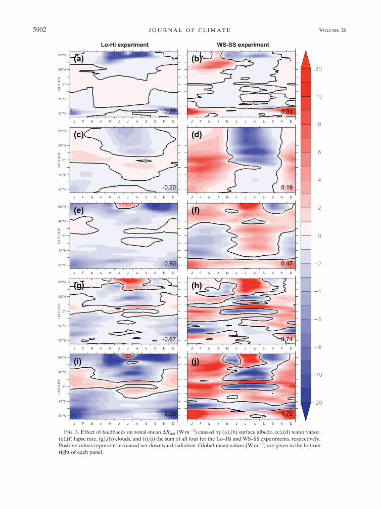
FIG. 9. Effect of feedbacks on zonal-mean DRnet (Wm22) estimated as the product of the doubled CO2 feedback

and the DT in each orbital experiment. As in Fig. 3, plots are shown for DRnet caused by (a),(b) surface albedo, (c),(d)

water vapor, (e),(f) lapse rate, (g),(h) clouds, and (i),(j) the sum of all four for the Lo–Hi and WS–SS experiments.

Positive values represent increased net downward radiation. Global-mean values (Wm22) are given in the bottom

right of each panel.

5908 JOURNAL OF CL IMATE VOLUME 26

account for this, areas where DTCO2is between20.5 and

10.5K have been masked out. However, the estimate is

still disproportionately affected by areas of low DTCO2,

so this section will focus primarily on differences in sign,

not magnitude, in the comparison of the actual (Fig. 3)

and estimated (Fig. 9) effect of feedbacks.

a. Lo–Hi experiment

Of the four feedbacks in the Lo–Hi experiment, the

surface albedo feedback shows the strongest similarities

between the actual and estimated response, suggesting

that changes in snow and sea ice are primarily associated

with local DT and do not rely heavily on other mecha-

nisms. While this is perhaps not surprising, it is inter-

esting to note that the actual and estimated responses

are similar, despite the opposite signs of high-latitude

DT in the Lo–Hi and CO2 experiments.

In the remaining feedbacks, differences are appar-

ent in the mid- to high latitudes during summer in both

hemispheres. The high-latitude changes stem from rel-

atively low DTCO2in the Southern Ocean and northern

Atlantic during their respective summers, where changes

in ocean circulation tend to reduce local warming in

global warming experiments (Stouffer et al. 2006) and in

the parts of Canada and Russia during NH summer,

where DTCO2is low because of increased precipitation

in the doubled CO2 experiment (Wetherald 2010). In-

creased precipitation throughout the year in these NH

high-latitude continental regions makes the soil wetter,

allowing increased evaporation during NH summer. This

decrease in the Bowen ratio diminishes local warming.

Because DT in the orbital experiments is not affected in

the same way in these regions, differences arise between

the actual and estimated feedback responses.

In the water vapor feedback, the calculated effect of

the water vapor feedback is larger at the equator and

smaller in the North African and Asian monsoon re-

gions than in the estimation. This difference is caused by

the enhanced Hadley circulation and a slight weakening

of those monsoons in the Lo–Hi experiment, both of

which rely more on the latitudinal temperature gradi-

ent than local DT alone. Monsoon changes also lead to

differences in the cloud feedback, as weaker NH mon-

soons result in local decreases in summer clouds. These

cloud feedbacks are not well reproduced in the estimated

response.

Outside of these regional variations, several wider-

scale differences should be addressed. In particular, the

calculated effects of the lapse rate and cloud feedbacks

are more negative than in the estimate, and the effect

of the water vapor feedback is more positive (Table 2).

One hypothesis to explain these differences involves the

transport of moist static energy (MSE) by the mean

meridional circulation. In theLo–Hi experiment, increases

in insolation at low latitudes produce positive MSE

anomalies through increases in surface air temperature

and specific humidity. Decreases in insolation at high

latitudes have the opposite effect. From a Lagrangian

perspective, the mean meridional circulation transports

low-latitude air upward and poleward, while air at the

poles is transported downward and equatorward. This

circulation should transport positive MSE anomalies

poleward in the upper troposphere and negative MSE

anomalies equatorward near the surface. This differen-

tial transport should have the effect of stabilizing the

atmosphere in the Lo–Hi experiment and affecting ra-

diative feedbacks in three important ways: 1) A de-

creased lapse rate emits more LW radiation to space,

cooling the climate; 2) a more stable atmosphere sus-

tains additional water vapor at height, increasing the

greenhouse effect and partially offsetting the primary

radiative effect of a decreased lapse rate; and 3) a more

stable atmosphere encourages increased cloud water

(Fig. 7), reflecting more insolation back to space. Thus,

despite potential changes in water vapor, the export of

high-latitude air with reduced MSE by the mean me-

ridional circulation may be responsible for pushing the

Lo–Hi experiment toward a colder global-mean climate.

This would allow regions of negative DT to be sustained

equatorward of the regions of negative insolation change,

as seen between approximately 208 and 408 latitude in

both hemispheres in the Lo–Hi experiment.

Outside of these important differences, however, many

aspects of the feedback responses remain relatively con-

sistent between the Lo–Hi and CO2 experiments. The

sign of the surface albedo and water vapor feedbacks is

consistent over most regions, as are the lapse rate and

cloud feedbacks outside of the midlatitudes, suggesting

that many aspects of the feedbacks depend upon the

local temperature change and are relatively insensitive

to the global distribution and type of forcing. Notably,

the dichotomy between the Arctic summer and fall

lapse rate responses in the Lo–Hi experiment is well

reproduced in the estimated feedback response, re-

inforcing the notion that this feature is a robust model

response largely dependent on local, rather than

global, processes.

This comparison between actual and estimated feed-

backs suggests that many aspects of feedbacks are a di-

rect response to local DT, but some aspects depend on

changes in atmospheric circulation. This is especially

apparent when comparing the total effect of feedbacks

(Figs. 3i, 9i), which show large-scale similarities as well

as some important differences. Table 2 lists global-mean

values of DRnet for both the actual and estimated re-

sponse. The surface albedo and water vapor responses

15 AUGUST 2013 ERB ET AL . 5909

are relatively similar, but the larger differences in the

lapse rate and cloud responses indicate complexities in

the relationship between feedbacks and the seasonal

and latitudinal pattern of temperature change.

b. WS–SS experiment

Comparing the actual and estimated responses in the

WS–SS experiment reveal large-scale similarities, but, as

in the Lo–Hi experiment, important differences become

apparent as well. For the water vapor feedback, the

greatest differences occur at low latitudes, mostly cor-

responding tomonsoonal changes, which are much larger

in the WS–SS experiment than the doubled CO2 experi-

ment. These large monsoonal changes in the WS–SS ex-

periment point to the importance of the seasonality of the

forcing. Because the thermal inertia of the ocean allows

the climate system to maintain a memory of forcing in

earlier seasons, previous seasonal changes may impact

later climate response. It is important to note, however,

that while NH and SHmonsoons produce changes in the

water vapor feedback that are of the opposite sign, these

anomalies are not of equal magnitude, making the ac-

tual DRnet from the water vapor feedback10.19Wm22,

while the estimated one is 10.61Wm22. Some of this

stems from the fact that changes in the North African

monsoon are more pronounced than changes in other

monsoons, significantly decreasing the water vapor over

northern Africa.

Monsoon changes also explain some of the differences

in the lapse rate and cloud feedbacks. In the lower lati-

tudes, less convectively active NH monsoons transport

less latent heat aloft, increasing the lapse rate over

northern Africa and the Indian subcontinent. The SH

monsoons have the opposite effect over South America,

southern Africa, and Australia during SH summer.

Monsoonal changes also reduce cloud water content

and cloud fraction over NH monsoon regions and in-

crease them over SH monsoon regions. These changes,

as well as the response of clouds to seasonal temperature

anomalies in the eastern equatorial Pacific, are not well

represented in the estimated response. This is apparent

when comparing the total effect of feedbacks (Figs.

3j, 9j), again pointing toward the importance of sea-

sonal variations in determining parts of the feedback

response.

Taking a step back, Table 2 shows that the latitudinal-

and seasonal-dependent response mechanisms outlined

above are important not just to aspects of localDRnet but

also to global DRnet. Therefore, the questions posed at

the beginning of this sectionmay be answered as follows:

1) There are many large-scale similarities between the

actual and estimated effect of the feedbacks, but also

crucial differences. 2) Important parts of the feedback

response cannot be understood as a simple response to

local DT. 3) Changes in systems such as the Hadley

circulation and monsoons are important to the global-

mean climate response.

6. Potential effect of feedbacks on expansionof NH ice sheets

According to orbital theory, low obliquity and peri-

helion at NH winter solstice (which are simulated sep-

arately in Lo–Hi and WS–SS) should promote NH ice

sheet growth by allowing high-latitude snow to survive

through cooler summers. Although the current experi-

ments cannot explicitly address the slow feedbacks that

are instrumental in amplifying the climate response to

orbital changes because of the absence of dynamic ice

sheets and biogeochemistry in CM2.1, the fast radiative

feedbacks can be evaluated to see whether they en-

courage high-latitude NH perennial snow cover in these

experiments or not.

Both Lo–Hi andWS–SS result in high-latitude cooling

during the NH summer, with Lo–Hi additionally cooling

at high latitudes year round (Fig. 2). Spatially, the NH

high-latitude summer DT is negative almost everywhere

in both experiments (Figs. 10a,b, shading), though the

WS–SS experiment has DT near zero over northern

ocean areas. Some of this pattern may be attributed

to the summer cloud feedback (Figs. 10a,b, contours),

which contributes positive DRnet over high-latitude

ocean regions and some continental regions in both

experiments. The total effect of feedbacks (not shown)

has the same sign as the cloud feedbacks over most lati-

tudes, enhancing cooling in some regions while dimin-

ishing it in others.

The NH high-latitude summerWS–SS cloud feedback

constitutes one of the largest feedbacks seen anywhere

in the orbital experiments and, as previously stated, in-

volves widespread decreases in cloud water content over

the majority of regions poleward of approximately 408Nassociated with decreased high-latitude summer stabil-

ity. Together with a decrease in low-cloud fraction over

the Arctic and northern ocean basins during July and

August (Fig. 6), this decrease in cloud water reduces

cloud albedo and allows a higher percentage of SW ra-

diation to reach the surface. The region of positiveDRnet

from the cloud feedback extends over parts of northern

Canada including Baffin Island, which remains one of

the most likely locations for past initiations of the Lau-

rentide Ice Sheet (Clark et al. 1993). This suggests that

the cloud feedback could partially counteract changes

in summer insolation at or near these regions at times

when the orbital configuration is favorable for ice sheet

expansion.

5910 JOURNAL OF CL IMATE VOLUME 26

However, despite the decreases in insolation and

continental temperature in both experiments, neither

experiment shows a widespread increase in perennial

snow cover, which would be the precursor to ice sheets.

Perennial snow cover remains confined to Greenland

and Antarctica, with the sole exception of a single point

over the Himalayas in the WS–SS experiment, which

maintains its snow throughout the cooler summer. An

analysis of melting degree-days, which indicate whether

snowmelt would increase or decrease over the course of

the year, shows that these experiments are still in agree-

ment with orbital theory. Figures 10c and 10d show that

melting degree-days are reduced over almost all conti-

nental regions poleward of 308N. Because continental

temperature can drop significantly below zero in winter,

melting degree-days are more affected by summer DT,which is negative in both experiments, than by winterDT,which is negative in the Lo–Hi experiment but positive in

the WS–SS experiment. These reductions in melting de-

gree-days should allow snow to remain on the ground

later in the melt season in both experiments.

Large-scale increases in perennial snow cover are not

expected in these experiments for several reasons: First,

the present experiments model low obliquity and NH

winter solstice perihelion forcing separately, while or-

bital theory suggests that both should be present to start

glaciations. Second, GFDL CM2.1 lacks the fine reso-

lution required to resolve the tall mountain peaks where

glaciations likely begin. Third, when comparing a mod-

ern run from GFDL CM2.1 against data from the

FIG. 10. (top) Mean June–August DT poleward of 308N in the (a) Lo–Hi and (b) WS–SS experiments (K; shaded).

Contours are the DRnet from the mean June–August cloud radiative feedback (Wm22). (bottom) Percent change in

annual melting degree-days over land for (c) Lo–Hi and (d) WS–SS. Melting degree-days are calculated from cli-

matological monthly values as the product of monthly temperature (for months that are above zero, in 8C) andnumber of days per month. White areas over Greenland remain below freezing year round, so they have no melting

degree-days in either simulation.

15 AUGUST 2013 ERB ET AL . 5911

Climatic Research Unit, version 2.1 (CRU v.2.1), temper-

ature dataset (Mitchell and Jones 2005), GFDL CM2.1

displays a warm bias of several degrees over northern

Canada and parts of northern Russia during NH sum-

mer. This warm bias increases the drop in temperature

needed to promote permanent snow cover in the CM2.1,

even if the first two reasons listed above are ignored.

As a final note, an open question remains regarding

how feedbacks may change as ice sheets grow. Changes

in surface type and elevation, both of which will happen

with expanding ice sheets, could have significant effects

on feedbacks. Snow feedbacks, which can be pronounced

over dark surfaces such as forests and grasslands, would

be much weaker over ice sheets, changing the regional

characteristics of the surface albedo feedback. The

lapse rate feedback will be affected by the much cooler

surface temperatures. Higher topography associated

with ice sheet growth may lead to a southward dis-

placement of the NH winter jet stream (Clark et al.

1999). Such changes in the atmospheric circulation and

topography may influence the cloud feedback. Because

of the complexity of these potential responses, feed-

backs that initially discourage or promote high-latitude

cooling may change with the growth of ice sheets. While

this topic deserves further research, analysis of those

potential responses is beyond the scope of the present

experiments.

7. Summary and conclusions

The role of orbital cycles in influencing past climate

variations has been the subject of much discussion over

the past decades, and understanding the role of feed-

backs in amplifying or damping that response remains

an intriguing question. To isolate and explore these

feedbacks, this study forced an AOGCM with idealized

orbital forcings, where obliquity and longitude of the

perihelion are varied without the competing effects of

changes in ice sheets and atmospheric composition. The

effects of feedbacks in these simulations were analyzed

and compared with those estimated from a doubled CO2

experiment to determine whether feedbacks behave con-

sistently under orbital and anthropogenic forcing. From

the results, the following statements may be made:

1) Global-mean climate change can result from a simple

redistribution of insolation, even when global-mean

insolation change is zero and radiative forcing is

small, because of the influence of radiative feed-

backs. Furthermore, DT does not have to be the

same sign as the radiative forcing, either locally or

globally, if the effects of feedbacks are sufficient to

overwhelm the direct radiative forcing.

2) The relative importance of each feedback to the

global-mean climate response is contingent on the

temporal and spatial distribution of the forcing.

While the water vapor feedback results in the largest

global-mean DRnet in the doubled CO2 experiment

(Table 2), it provides the smallest global-mean

DRnet in both orbital experiments. The lapse rate

and cloud feedbacks prove most important in both

orbital experiments, together accounting for over

70% of the global-mean DRnet from feedbacks.

3) While many aspects of the feedbacks may be consid-

ered a simple response to local DT, some are not,

especially in the water vapor, lapse rate, and cloud

feedbacks. Circulation changes, which are largely

dependent on the seasonal and spatial patterns of

forcing, affect regional feedbacks in important ways.

Monsoon circulations are especially important, play-

ing a large role in influencing WS–SS feedbacks

and a smaller role in influencing Lo–Hi feedbacks.

4) Vertical variations in themeridional transport ofMSE

anomalies may play a role in extending the reach of

local climate anomalies to more distant areas. In the

Lo–Hi experiment, increases in MSE in the tropics

may be transported poleward at altitude while neg-

ative MSE anomalies from the high latitudes are

transported equatorward near the surface, increas-

ing the large-scale stability of the atmosphere and

encouraging global-mean cooling through impacts

on the lapse rate and cloud feedbacks.

5) Cloud feedbacks partially counteract changes in sum-

mer insolation over someNH high-latitude ocean and

continental regions during times most favorable for

ice sheet expansion.However, it is unclear how clouds

would react to ice sheet expansion or reduction as the

CM2.1 lacks dynamic ice sheets.

These results emphasize the significant role of radiative

feedbacks in shaping orbitally forced climate change.

Undoubtedly, feedbacks have played a large role in in-

fluencing climate in the past and will continue to do so

in the coming century. Better understanding of how these

feedbacks operate under a variety of forcings may help us

understand what role feedbacks will play in the future.

Acknowledgments. This research was supported by

the Paleo Perspectives on Climate Change program of

the National Science Foundation (GrantATM0902735).

The authors would like to extend their thanks to F. Zeng

and J. Krasting for their help in conducting these simu-

lations; B. Soden for use of the radiative kernels and

CMIP3 calculations; D. Pollard for help with the cal-

endar conversion; V. Ghate, J. Kay, and N. Barton for

their cloud expertise; and the NOAAGeophysical Fluid

5912 JOURNAL OF CL IMATE VOLUME 26

Dynamics Laboratory at Princeton for use of their com-

puting resources. Additionally, we thank two anonymous

reviewers for their useful comments.

REFERENCES

Anderson, J. L., and Coauthors, 2004: The new GFDL global at-

mosphere and land model AM2–LM2: Evaluation with pre-

scribed SST simulations. J. Climate, 17, 4641–4673.

Berger, A., and M. F. Loutre, 1991: Insolation values for the cli-

mate of the last 10 million years. Quat. Sci. Rev., 10, 297–317.

Bony, S., and Coauthors, 2006: How well do we understand and

evaluate climate change feedback processes? J. Climate, 19,

3445–3482.

Chen, G.-S., J. E. Kutzbach, R. Gallimore, and Z. Liu, 2010: Cal-

endar effect on phase study in paleoclimate transient sim-

ulation with orbital forcing. Climate Dyn., 37, 1949–1960,

doi:10.1007/s00382-010-0944-6.

Clark, P. U., and Coauthors, 1993: Initiation and development of

the Laurentide and Cordilleran ice sheets following the last

interglaciation. Quat. Sci. Rev., 12, 79–114, doi:10.1016/

0277-3791(93)90011-A.

——, R. B. Alley, and D. Pollard, 1999: Northern Hemisphere ice-

sheet influences on global climate change. Science, 286, 1104–

1111, doi:10.1126/science.286.5442.1104.

Clement, A. C., A. Hall, and A. J. Broccoli, 2004: The importance

of precessional signals in the tropical climate. Climate Dyn.,

22, 327–341, doi:10.1007/s00382-003-0375-8.——,R. Burgman, and J. R. Norris, 2010: Response to comment on

‘‘Observational andmodel evidence for positive low-level cloud

feedback.’’ Science, 329, 277, doi:10.1126/science.1187667.Colman, R., 2003: A comparison of climate feedbacks in general

circulation models. Climate Dyn., 20, 865–873, doi:10.1007/

s00382-003-0310-z.

Delworth, T. L., and Coauthors, 2006: GFDL’s CM2 global cou-

pled climate models. Part I: Formulation and simulation

characteristics. J. Climate, 19, 643–674.

Fleitmann, D., and Coauthors, 2007: Holocene ITCZ and Indian

monsoon dynamics recorded in stalagmites from Oman and

Yemen (Socotra). Quat. Sci. Rev., 26, 170–188, doi:10.1016/

j.quascirev.2006.04.012.

Hall, A., 2004: The role of surface albedo feedback in climate.

J. Climate, 17, 1550–1568.

——, A. C. Clement, D. W. J. Thompson, A. J. Broccoli, and C. S.

Jackson, 2005: The importance of atmospheric dynamics in the

NorthernHemisphere wintertime climate response to changes

in the earth’s orbit. J. Climate, 18, 1315–1325.

Hays, J. D., J. Imbrie, and N. J. Shackleton, 1976: Variations in

the earth’s orbit: Pacemaker of the ice ages. Science, 194,

1121–1132.

Herweijer, C., R. Seager, M. Winton, and A. Clement, 2005: Why

ocean heat transport warms the global mean climate. Tellus,

57A, 662–675.

Huybers, P., 2006: Early Pleistocene glacial cycles and the in-

tegrated summer insolation forcing. Science, 313, 508–511,

doi:10.1126/science.1125249.

——, and E. Tziperman, 2008: Integrated summer insolation

forcing and 40,000-year glacial cycles: The perspective from

an ice-sheet/energy-balance model. Paleoceanography, 23,

PA1208, doi:10.1029/2007PA001463.

Imbrie, J., andCoauthors, 1993: On the structure and origin ofmajor

glaciations cycles 2. The 100,000-year cycle. Paleoceanography,

8, 699–735.

Jackson, C. S., and A. J. Broccoli, 2003: Orbital forcing of Arctic

climate: Mechanisms of climate response and implications

for continental glaciations. Climate Dyn., 21, 539–557,

doi:10.1007/s00382-003-0351-3.

Joussaume, S., and P. Braconnot, 1997: Sensitivity of paleoclimate

simulation results to season definitions. J. Geophys. Res., 102

(D2), 1943–1956.

Jouzel, J., and Coauthors, 2007: Orbital and millennial Antarctic

climate variability over the past 800,000 years. Science, 317,

793–796, doi:10.1126/science.1141038.

Khodri, M., M. A. Cane, G. Kukla, J. Gavin, and P. Braconnot,

2005: The impact of precession changes on the Arctic climate

during the last interglacial–glacial transition.Earth Planet. Sci.

Lett., 236, 285–304, doi:10.1016/j.epsl.2005.05.011.

Lee, S.-Y., and C. J. Poulsen, 2005: Tropical Pacific climate re-

sponse to obliquity forcing in the Pleistocene. Paleoceanog-

raphy, 20, PA4010, doi:10.1029/2005PA001161.

——, and ——, 2008: Amplification of obliquity forcing through

mean annual and seasonal atmospheric feedbacks. Climate

Past, 4, 515–534, doi:10.5194/cpd-4-515-2008.

Manabe, S., and R. J. Stouffer, 1980: Sensitivity of a global climate

model to an increase of CO2 concentrations in the atmo-

sphere. J. Geophys. Res., 85 (C10), 5529–5554.

Mantsis, D. F., A. C. Clement, A. J. Broccoli, and M. P. Erb, 2011:

Climate feedbacks in response to changes in obliquity. J. Cli-

mate, 24, 2830–2845.Meehl, G. A., C. Covey, T. Delworth, M. Latif, B. McAvaney, J. F.

B. Mitchell, R. J. Stouffer, and K. E. Taylor, 2007: TheWCRP

CMIP3 multimodel dataset: A new era in climate change re-

search. Bull. Amer. Meteor. Soc., 88, 1383–1394.Milankovitch, M., 1941: Kanon der Erdbestrahlung und seine An-

wendung auf das Eiszeitenproblem (Canon of Insolation and

the Ice-Age Problem). Royal Serbian Academy, Special Pub-

lication, Vol. 133, 633 pp.

Mitchell, T. D., and P. D. Jones, 2005: An improved method of

constructing a database of monthly climate observations and

associated high-resolution grids. Int. J. Climatol., 25, 693–712,

doi:10.1002/joc.1181.

Otto-Bliesner, B., and A. C. Clement, 2004: The sensitivity of the

Hadley circulation to past and future forcings in two climate

models. The Hadley Circulation: Present, Past and Future,H. F.

Diaz and R. S. Bradley, Eds., Advances in Global Change

Research Series, Vol. 21, Springer Verlag, 437–464.

Petit, J. R., and Coauthors, 1999: Climate and atmospheric history

of the past 420,000 years from the Vostok ice core, Antarctica.

Nature, 399, 429–436.

Phillipps, P. J., and I. M. Held, 1994: The response to orbital per-

turbations in an atmospheric model coupled to a slab ocean.

J. Climate, 7, 767–782.Pollard, D., and D. B. Reusch, 2002: A calendar conversion

method for monthly mean paleoclimate model output with

orbital forcing. J. Geophys. Res., 107, 4615, doi:10.1029/

2002JD002126.

Prell,W. L., and J. E. Kutzbach, 1987:Monsoon variability over the

past 150,000 years. J. Geophys. Res., 92 (D7), 8411–8425.

Ramaswamy, V., and Coauthors, 2001: Radiative forcing of cli-

mate change. Climate Change 2001: The Scientific Basis, J. T.

Houghton et al., Eds., Cambridge University Press, 349–416.

Raymo, M. E., and K. Nisancioglu, 2003: The 41 kyr world: Mi-

lankovitch’s other unsolved mystery. Paleoceanography, 18,

1011, doi:10.1029/2002PA000791.

Reichler, T., and J.Kim, 2008:Howwell do coupledmodels simulate

today’s climate? Bull. Amer. Meteor. Soc., 89, 303–311.

15 AUGUST 2013 ERB ET AL . 5913

Rind, D., and J. Perlwitz, 2004: The response of the Hadley circu-

lation to climate changes, past and future. The Hadley Circu-

lation: Present, Past and Future, H. F. Diaz and R. S. Bradley,

Eds., Advances in Global Change Research Series, Vol. 21,

Springer Verlag, 399–435.

Robock, A., 1983: Ice and snow feedbacks and the latitudinal and

seasonal distribution of climate sensitivity. J. Atmos. Sci., 40,

986–997.

Soden, B. J., and I. M. Held, 2006: An assessment of climate

feedbacks in coupled ocean–atmosphere models. J. Climate,

19, 3354–3360.

——, and G. A. Vecchi, 2011: The vertical distribution of cloud

feedback in coupled ocean-atmospheremodels.Geophys. Res.

Lett., 38, L12704, doi:10.1029/2011GL047632.

——, A. J. Broccoli, and R. S. Hemler, 2004: On the use of cloud

forcing to estimate cloud feedback. J. Climate, 17, 3661–

3665.

——, I. Held, R. Colman, K.M. Shell, J. T. Kiehl, andC. A. Shields,

2008: Quantifying climate feedbacks using radiative kernels.

J. Climate, 21, 3504–3520.

Stouffer, R. J., and Coauthors, 2006: GFDL’s CM2 global coupled

climate models. Part IV: Idealized climate response. J. Cli-

mate, 19, 723–740.Timm, O., A. Timmerman, A. Abe-Ouchi, F. Saito, and T. Segawa,

2008: On the definition of seasons in paleoclimate simula-

tions with orbital forcing. Paleoceanography, 23, PA2221,

doi:10.1029/2007PA001461.

Timmermann, A., S. J. Lorenz, S.-I. An, A. C. Clement, and S.-P.

Xie, 2007: The effect of orbital forcing on the mean climate and

variability of the tropical Pacific. J. Climate, 20, 4147–4159.

Tuenter, E., S. L. Weber, F. J. Hilgen, and L. J. Lourens, 2003: The

response of the African summer monsoon to remote and local

forcing due to precession and obliquity. Global Planet.

Change, 36, 219–235, doi:10.1016/S0921-8181(02)00196-0.——,——,——, and——, 2005a: Sea-ice feedbacks on the climatic

response to precession and obliquity forcing. Geophys. Res.

Lett., 32, L24704, doi:10.1029/2005GL024122.

——, ——, ——, ——, and A. Ganopolski, 2005b: Simulation of

climate phase lags in response to precession and obliquity

forcing and the role of vegetation. Climate Dyn., 24, 279–295,

doi:10.1007/s00382-004-0490-1.

Wang, Y., and Coauthors, 2008: Millennial- and orbital-scale

changes in the East Asian monsoon over the past 224,000

years. Nature, 451, 1090–1093, doi:10.1038/nature06692.

Wetherald, R. T., 2010: Changes of time mean state and vari-

ability of hydrology in response to a doubling and quadru-

pling of CO2. Climatic Change, 102, 651–670, doi:10.1007/

s10584-009-9701-4.

Wyrwoll, K.-H., Z. Liu, G. Chen, J. E. Kutzbach, and X. Liu, 2007:

Sensitivity of the Australian summer monsoon to tilt and

precession forcing.Quat. Sci. Rev., 26, 3043–3057, doi:10.1016/

j.quascirev.2007.06.026.

Yoshimori, M., and A. J. Broccoli, 2008: Equilibrium response of

an atmosphere–mixed layer oceanmodel to different radiative

forcing agents: Global and zonal mean response. J. Climate,

21, 4399–4423.Ziegler, M., E. Tuenter, and L. J. Lourens, 2010: The precession

phase of the boreal summer monsoon as viewed from the

eastern Mediterranean (ODP site 968). Quat. Sci. Rev., 29,

1481–1490, doi:10.1016/j.quascirev.2010.03.011.

5914 JOURNAL OF CL IMATE VOLUME 26