The cost of default in a cash-in-advance economy Kwangwon Ahn ∗ , Daeyong Lee † and Shasha Li ‡ 2018 May Abstract The 2008 global financial crisis and its aftermath caused the high default rate and thus many national central banks ran expansionary monetary policy. Under a Cash- In-Advance (CIA) framework, we examine the welfare cost of default and how the injection of cash affects welfare cost of default. Incorporating non-linear form of non- pecuniary default penalty into a CIA model, we find that default causes around 1% loss in consumption. The negative effects of default on welfare is significantly greater in an economy with higher money growth rate only in the long-run but not in the short-run. Keywords: Welfare cost; Default; Monetary Policy; Cash-In-Advance JEL Classification: E44; E52; G01; I30 ∗ Korea Advanced Institute of Science and Technology, [email protected]† Iowa State University, [email protected]‡ Bocconi University, [email protected]1
Transcript
The cost of default in a cash-in-advance economy
Kwangwon Ahn∗ , Daeyong Lee† and Shasha Li‡
2018 May
Abstract
The 2008 global financial crisis and its aftermath caused the high default rate andthus many national central banks ran expansionary monetary policy. Under a Cash-In-Advance (CIA) framework, we examine the welfare cost of default and how theinjection of cash affects welfare cost of default. Incorporating non-linear form of non-pecuniary default penalty into a CIA model, we find that default causes around 1% lossin consumption. The negative effects of default on welfare is significantly greater in aneconomy with higher money growth rate only in the long-run but not in the short-run.
1 IntroductionThe recent financial crisis in 2008 caused a high level of default rate. In 2009, Moody’s
global speculative-grade default rate peaked 13 percent, and it was followed by a globaleconomic downturn. For example, the U.S. personal consumption expenditure fell below92 percent of disposable personal income as of 2009. To escape from the Great Recessionin 2008, the US government implemented the expansionary monetary policy, known as“Quantitative Easing” during 2009 and 2010. It added around $2 trillion to the moneysupply. Although the coexistence of widespread default in the credit market and a largeinjection of cash was unprecedent in the U.S. financial crisis history, little studies have beendone evaluating the effects of both default and monetary policy on social welfare.
As such, we estimate the welfare cost of default and investigate how the welfare cost ofdefault varies with abnormal money injection. First, to assess the welfare cost of default, webuild a Dynamic Stochastic General Equilibrium (DSGE) model incorporating both Cash-In-Advance (CIA) constraints and endogenous default. The welfare cost is measured as thepercentage change in real consumption, to maintain the same level of utility with that inthe benchmark economy without default (Lucas, 1987; Cooley and Hansen, 1989). Second,we measure default rate as the probability of not repaying at all, and construct defaultpenalty as a non-linear form of utility loss. The default penalty increases non-linearly withthe default volume and credit-regulation level. Third, to model the money supply rule, weuse AR (1) process on money growth rates. This simplified monetary supply rule reflectsthe fact that the Federal Reserve Board implemented a policy by maneuvering quantitiessince interest rates were too low to drop (Adrian and Shin 2009).
Using the theoretical framework, we find that default reduces social welfare. Default riskreduces corporate loan volume, which leads to lower investment and output. As a result,households consume less. The presence of default causes social welfare loss by around 1% lossin consumption. Since firms bear the deadweight loss of default, stricter credit-regulationwill lower default rate and improve social welfare at the cost of lower firm profits.
In addition, we find that the welfare cost of default increases with money growth rate, andthis negative effect of the expansionary monetary policy on the welfare cost is nonnegligiblein the long-run. Because the time is long enough to accumulate the propagation effectcaused by default in credit market to significantly reduce the consumption. It is more socialwelfare costly for a CIA economy with higher money growth rate. However, in the shortrun, this propagation effect is small, and thus the welfare cost is not significant. This maylead to monetary policy inertia. The policy maker may not respond to the default behaviorquickly enough if they haven’t observed a significant welfare loss.
To our best of knowledge, this article is the first study that assesses the welfare costof default by incorporating with monetary policy. Since the 2008 global financial crisis,many governments have implemented expansionary monetary policy to recover the bustedeconomy. Thus, to incorporate the government monetary policy into a model providesthe more comprehensive understanding the welfare cost of default. In literature, mostresearch about cost of default emphasized the profit loss to individual firms (Warner, 1977;Altman, 1984; Weiss, 1990; Davydenko et al., 2012; Glover 2016). The welfare cost ofdefault haven’t been studied thoroughly, let alone how monetary policy affects welfare cost ofdefault. The findings in our study help policymakers consider in which way they implementtheir monetary policy to cope with a financial crisis with high default rates. Furthermore,this study contributes to the literature of CIA models to overcome the limitation of standardCIA models. Standard CIA models are not feasible to generate the positive response of
2
output to unexpected money growth shock. To overcome this limitation, we use a non-linearform of non-pecuniary default penalty. With the existence of non-linear default penalty,default rate is lower and lower default risk premium boosts lending in the corporate loanmarket and result in higher output.
The structure of this paper is as follows. Section 2 reviews past literature. Section 3presents our model, which forms the basis for our analysis. Section 4 lays down equilibriumanalysis such as market clearing conditions and optimality conditions. Section 5 explainscalibration of the model. Section 6 discusses our results based on quantitative analysis,including cyclical properties, steady states and estimation of welfare costs of default in oureconomy. Sections 7 provides conclusions.
2 Literature reviewThis paper relates to several streams of studies in the literature.
2.1 Monetary models with CIA constraintsThere’s a wide agreement in the macroeconomics literature that nominal or monetary
factors is important since Lucas (1972, 1973, 1975). To further theoretically study the roleof money, Lucas (1982) and Lucas and Stokey (1987) initiated the “cash-in-advance mod-els” where goods can be identified as distinctive “credit goods” or “cash goods” dependingon timing and agents hold money due to “cash-in-advance constraints” (Clower, 1967) forbuying “cash goods”. The Clower type CIA constraint implies that agents must have enoughcash balance before they can purchase “cash goods”, and it captures the role of money asa medium of exchange. Following basic framework of Lucas and Stokey (1987) and Hansen(1985), Cooley and Hansen (1989) introduced money into the “Real Business Cycle model”.It revealed the co-movements between real and nominal economic variables and claimedthat the anticipated inflation tax induced by money supply growth causes huge social wel-fare loss. After that, CIA models became a popular approach to model money in dynamicmacroeconomic framework because it is a simple way to model money demand and reflectany surprise in monetary policy.
But monetary RBC models with CIA constraints have some drawbacks in monetarypolicy effects analysis. According to Schorfheide (2000), monetary RBC models with CIAconstraints fail to generate positive response of real output to an unanticipated positiveshock in monetary policy. It suggests that in order to successfully account for the interactionbetween real and nominal variables, more sources of non-neutrality than just the inflationtax should be considered.
2.2 Financial frictions in macroeconomicsFinancial frictions came into macro economists’ view since Bernanke and Gertler (1989)’s
overlapping-generations model. Bernanke and Gertler (1989) started from informationasymmetry, to model financial friction. After that, there are mainly two approaches tointroduce financial frictions into the general equilibrium framework.
The first approach is explored by Kiyotaki and Moore (1997) which is based on collateralconstraints and emphasizes more on the quantity of loans. In their model, lenders are notallowed to force borrowers to fulfill their obligations, and borrowers cannot borrow moneyunless their debts are secured. Generally, durable assets are used as collateral for loans.
3
Financial markets have influence on real economic activities through interaction betweendurable asset prices and credit limitation. Many applications based on this frameworkappeared after that. Iacoviello (2005) introduced housing as collateral and more recentlyGerali et al. (2010) assumed that the inter-bank financing ability of banks is limited by theasset portfolio available for collateral to study the impact of financial frictions on monetarypolicy transmission.
The other approach is a continue of Bernanke-Gertler agency-costs economy which ac-centuates the role of external finance premium. Carlstrom and Fuerst (1997) extendedBernanke-Gertler model to infinite time horizon and later Bernanke et al. (1999) mergedthis approach with the New-Keynesian framework, which became a classical reference forfinancial frictions modelling. In this type model, borrowers and lenders are different withconflict of interest, leading to agency problem. Monitoring the credit market is costly,and agency costs are constructed as endogenous. Financial markets affects business cyclesmainly through the prices of loans in which credit risk premium is considered. Christianoet al. (2004), Christiano et al. (2007) and Christiano et al. (2008) further used the externalfinance premium setup to study the role of financial frictions in business cycles. In thispaper, the external finance premium approach is adopted to study the role of default.
2.3 Default and cost of defaultAmong all possible financial frictions, Goodhart et al. (2006) and Tsomocos (2003) sug-
gested to mainly concentrate on two factors, money and default, to study the monetarymechanism and financial stability. Shubik and Wilson (1977) first introduced the the possi-bility of default as equilibrium phenomenon that borrowers can choose the optimal fractionof debts to repay. Following this setup, Goodhart et al. (2006), Tsomocos (2003), and Tso-mocos and Zicchino (2005) modelled endogenous default into the economy to study the roleof default in monetary mechanism. Agents are allowed to choose their repayment rates,and thus equilibrium in such economy is compatible with complete or partial abrogation ofborrowers’ obligations. If it is not worthy to repay any of their debts, agents will rationallydefault all.
Then introduction of the cost of default is important. To fully define all possible out-comes in strategic market games, Shapley and Shubik (1977) introduced minimal institutionssuch as money, credit and default, and the rules of default penalties to be levied againstagents who choose to default. Geanakoplos (1997) proposed to model penalties of defaulton secured debts as pecuniary penalty based on the loss of collateral, which at least guar-antees partial payment; while default on unsecured debts are constructed as pecuniary lossor non-pecuniary loss. The pecuniary penalties can be considered as garnishing of futureincome or a search cost for new financial resources, and the non-pecuniary default can beconsidered as pangs of conscience, a prison term or reputation loss. In the field of non-pecuniary default penalty, Tsomocos (2003) is one of the papers that pioneer to incorporatedefault penalties on borrowers into general equilibrium framework and constructed the costof default as a default penalty that reduces the borrowers’ utilities. Dubey et al. (2005)imposed a default penalty in the form of reputation loss in a multi-period world which willmake agents keep their promises to pay back their debts. The default firms fear to lose newfinancing opportunities in the future. In addition, according to Dubey et. al (2005), thedefault penalty generally increases with the nominal amount of default.
Until now, there are very few articles that study the welfare cost of default and thewelfare consequences are ambiguous according to the literature. In Dubey et al. (2000)
4
and Dubey et al. (2005) default causes social benefit in the incomplete market setting byenlarging asset span. While in Barro (1976) default causes net social welfare loss due tothe asymmetric information between the borrower and lender. In their setting, default on aloan triggers the loss of collateral value to the borrower, making the lender valuation muchbelow borrower valuation during the negotiation.
The finding of this paper is consistent with the second stream of the literature (e.g.,Barro 1976) that default on a loan causes net social welfare loss and it contributes to theliterature by estimating the magnitude of the welfare consequence.
3 The modelThis section describes the established simple dynamic stochastic general equilibrium
(DSGE) model with infinite time horizon. This model is extracted and extended from theCIA monetary DSGE model in Schorfheide (2000). In this economy, there are two agents,representative households and firms. Each household is identical, and so is each firm. Therepresentative household and firm live forever. Households are endowed with labor, inheritthe entire money stock of the economy from last period, and obtain utility from enjoyingleisure and consumption. Firms use labor and capital to produce and sell final goods, andobtain utility from profits. Firms are owned by households, and thus in the end of eachperiod, firms distribute all their profits to households in the form of dividends.
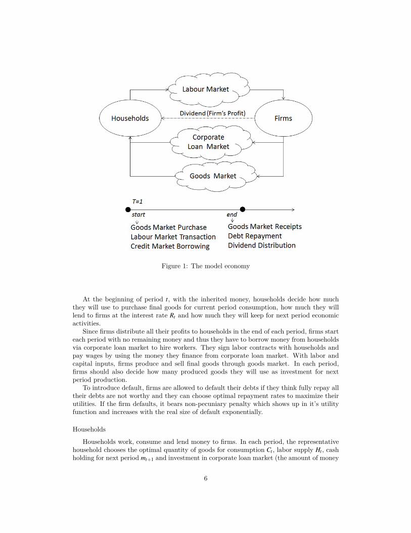
Households face CIA constraints. Before they purchase consumption goods, they shouldhave enough money (cash) in their hands. So consumption goods is “cash goods” in thiseconomy. The setup of CIA constraints enable the economy completely reflect the currentperiod’s surprise in technology and money supply growth. Money is fiat and thus holdingidle money in hand does not generate any utility for agents. They will lend all the idlemoney out to someone who need it. Figure 1 presents the diagram of the model economy.Households and firms play their roles in goods market, credit market, labor market andcorporate loan market. The nominal price level, Pt , is subject to the interplay of demandand supply in the final goods market.
5
Figure 1: The model economy
At the beginning of period t, with the inherited money, households decide how muchthey will use to purchase final goods for current period consumption, how much they willlend to firms at the interest rate Rt and how much they will keep for next period economicactivities.
Since firms distribute all their profits to households in the end of each period, firms starteach period with no remaining money and thus they have to borrow money from householdsvia corporate loan market to hire workers. They sign labor contracts with households andpay wages by using the money they finance from corporate loan market. With labor andcapital inputs, firms produce and sell final goods through goods market. In each period,firms should also decide how many produced goods they will use as investment for nextperiod production.
To introduce default, firms are allowed to default their debts if they think fully repay alltheir debts are not worthy and they can choose optimal repayment rates to maximize theirutilities. If the firm defaults, it bears non-pecuniary penalty which shows up in it’s utilityfunction and increases with the real size of default exponentially.
Households
Households work, consume and lend money to firms. In each period, the representativehousehold chooses the optimal quantity of goods for consumption Ct , labor supply Ht , cashholding for next period mt+1 and investment in corporate loan market (the amount of money
6
lend to firms) Dt to maximize the expected sum of discounted lifetime utility. As a result,it solves the optimization problem as follows,
max{Ct ,Ht ,mt+1,Dt}
E0
∞
∑t=0
βt {(1−ϕ) lnCt +ϕ ln(1−Ht)}
s.t.
PtCt ≤ mt −Dt +WtHt +(gt −1)Mt (1)0 ≤ Dt (2)
mt+1 = (mt −Dt +WtHt +(gt −1)Mt −PtCt)+νtRtDt +Ft (3)where E0(·) is the expectation operator conditional on date 0, β refers to the discount factor,ϕ is the preference shifter which reflects the marginal rate of substitution between leisureand consumption, νt is the repayment rate determined by the firm, Wt is the nominal wage,Ft is the dividend coming from firms, Mt denotes the per capita money supply in periodt −1, and the money stock in this economy follows a law of motion Mt+1 = gtMt .
The first constraint the household faces is the CIA constraint. The household hasmoney inflow from last period money stock inheritance mt , current period money injec-tion (gt −1)Mt , wage revenues WtHt . At the same time, s/he lends money Dt out to firmsand purchases consumption goods with expenditure PtCt . The money used for consumptioncannot exceed the household’s money balance mt −Dt +WtHt +(gt −1)Mt .
The second constraint means the representative household cannot borrow money fromfirms. Households have no debts outstanding.
The third constraint is the inter-temporal budget. Other than the remaining moneybalance after consumption, the household gets money from the firm in the end of eachperiod. As a creditor, the household gets repayment with the amount of νtRtDt from thefirm; as a owner, the household received cash dividend distribution from the firm with theamount of Ft .
Firms
Firms borrow money from households, hire workers and produce goods. They issuecorporate bond to hire workers in the beginning of each periods, and pay back optimalfraction of their debts outstanding in the end of each period. Specially firms are allowedto default at the cost of non-pecuniary penalty. To balance the benefits and costs of thedefault, firms will choose their optimal repayment rates.
Firms use labor and capital to produce goods. Final goods are produced following a“Cobb-Douglas production function”,
Yt = Kαt (AtNt)
1−α (4)where Kt denotes the capital stock which is predetermined at the beginning of period t, Atis a labor-augmenting technology and Nt represents the labor input. α and (1−α) representoutput elasticity of capital and output elasticity of labor respectively.
Capital is accumulated according to the law of motion Kt+1 = (1−δ)Kt + It (0 < δ < 1) ,where It is the new investment in current period.
In each period, the representative firm should make optimal decisions on labor demandNt , bond issued Lt , repayment rate νt , nominal cash dividends Ft , and the next period’scapital stock Kt+1. Since households receive the dividend in the end of each period, andthus value a unit of nominal cash dividend in terms of purchase power in next period.Firms distribute all their profits to households in the end of each period, so the current
7
period nominal dividends are discounted by marginal utility of consumption in next period.Moreover, firms care about the default penalties to be levied on them.
To be brief, the representative firm faces the optimization problem as follows,
max{Ft ,Kt+1,Nt ,Lt ,νt}
E0
∞
∑t=0
βt+1
{Ft
Ct+1Pt+1− ι
1+η
[(1−νt)Rt
Lt
Mt
]1+η}
s.t.WtNt ≤ Lt (5)
Ft = Lt +Pt
[Kα
t (AtNt)1−α −Kt+1 +(1−δ)Kt
]−WtNt −νtRtLt (6)
where ι and η denote the coefficient and the elasticity of non-pecuniary default for firms.When ι is higher, the regulation in the credit market is stricter and thus firms hesitate
more when they make a decision to default. When η is higher, the default penalty increasesmore quickly with the real size of default, and the firm cares more about negative effects ofdefault. To some extent, ι can be explained as the degree of default regulation and η canbe explained as the firm’s degree of risk-aversion.
The first constraint shows that the firm borrow money from households through corpo-rate bond to pay wages to workers at the beginning of each period.
The second constraint shows that the firm obtains the sales revenue, repays νtRtLt tohouseholds, invests more for next period production and distributes the remaining cash tohouseholds as the dividend.
Note that since money supply growth rate is greater than discount factor, CIA constraintsand budget constraints for both households and firms are binding.
Technology is assumed to follow a stationary AR(1) process,lnAt = ρA lnAt−1 +(1−ρA) ln A+σAεA,t (7)εA,t ∼ i.i.d. N(0,1)
ρA refers to the AR(1) coefficient of technology and A indicates the steady state of technology.The innovation εA,t follows a N(0,1) process where σA denotes the standard deviation ofinnovations to lnAt .
Monetary policy
The money growth rate in current period is defined as gt = Mt+1/Mt , where Mt is themoney supply in period t − 1. In each period, the central bank injects (gt −1)Mt moneyinto this economy. To make our analysis simple and straightforward, it is assumed that theinter-temporal money growth rate is stable in the long run and the log-linearized forms ofgt follows a stochastic AR(1) process,
Where g is unconditional mean, εg,t is the innovations to the monetary policy which follows astandard normal process, and σg measures the standard deviation of monetary innovations.Thus, the last term σgεg,t captures the unexpected monetary policy shock due to suddennominal policy making.
Equation (8) can be interpreted as a simple monetary policy rule without feedback. Themonetary policy shock is modeled as exogenous to investigate the transmission mechanism.
There are three markets in this economy: labor market, corporate loan market and finalgoods market. It is assumed that all markets are competitive. Thus, in the model economies,an equilibrium requires clearing all three markets.
For the labor market, the market clears when the supply of labor from households isequal to the demand of the labor from firms. Thus, Ht = Nt holds for ∀t ∈ T .
For the corporate loan market, the amount of money that households are willing to lendis equal to the amount of money that firms need for paying wages. Thus, Dt = Lt holds for∀t ∈ T .
Note that in equilibrium, the money supply equals to the money demand, mt = Mt .For the final goods market, the market clearing condition is that the demand for final
goods from consumption and investment equals to the supply of final goods produced byfirms. Thus, Ct + It = Yt holds for ∀t ∈ T . This market clearing condition can be derivedfrom the budget constraint of households (3) and the budget constraint of firms (6), alongwith labor and money market equilibrium conditions.
Recall all budget the constraints of households and firms are binding. In an equilibrium,when we combine budget constraints (1) and (5),
PtCt = mt −Lt +WtNt +(gt −1)Mt
WtNt = Lt
In equilibrium, money supply is epitomized, thus Mt = mt . Then it further implies theequilibrium condition in the money market,
PtCt = Mt+1 (9)According to the equation (9), the money demand which is denoted by nominal con-
sumption demand PtCt should be equal to money supply Mt+1, which can be represented bycurrent nominal balances mt and monetary injections (gt −1)Mt .
4.2 Optimality conditionsThis part shows the results of optimality conditions derived from the optimization prob-
lems of households and firms face to give us some characteristics of this cash-in-advanceeconomy with default.
According to the optimality condition for money market, PtCt = Mt+1, it shows that inthe long run money is neutral in this model economy, which is in line with the argument inreal business cycle (RBC) theory and New Keynesian literature. However, in the short run,money is not neutral in this artificial economy, which is in contrast with the standard RBCtheory.
One thing should be clarified here is that the mechanism leading to short run moneynon-neutrality in this artificial cash-in-advance economy differs from that in New Keynesianframework. In this economy, money non-neutrality is driven by transaction demands formoney and the financing channel where money and default have great influence; while underNew Keynesian framework, real frictions such as monopolistic or asymmetric informationare important.
According to the first order conditions (FOCs) derived from optimization problem ofhouseholds, we can easily get following equations:
9
ϕCtPt
(1−ϕ)(1−Ht)−Wt = 0 (10)
Et
(βνtRt
Ct+1Pt+1
)− 1
CtPt= 0 (11)
The optimality condition (10) shows that the marginal rate of substitution (MRS) be-tween consumption and leisure must be equal to the nominal wage rate. The optimalitycondition (11) represents the stochastic consumption Euler equation: the marginal utility ofconsumption in current period should be equal to the expected weighted marginal utility ofconsumption in next period. In other words, it means if they do not consume today and lendout the money, the marginal utility of consumption today is equivalent to the discountedmarginal utility of next period consumption enabled by the money received from repayment.
From this model, it also shows that the labor market optimality condition are closelyassociated with the credit market and households’ consumption decision. One possibleexplanation is that firms have to borrow money through credit market (corporate loanmarket) to pay wage bills. So their financing ability will affect the demand side of thelabor market. In detail, the optimality condition can be derived from combining the firm’sborrowing constraint Lt =WtNt , labor market equilibrium Ht = Nt and Dt = Lt and FOCs,
ϕCtPt
(1−ϕ)(1−Nt)− Lt
Nt= 0 (12)
Equation (12) suggests that when the ratio of money invest in corporate loan marketand expenditure used in consumption goods purchase increases, there will be more workersemployed in the labor market.
For the maximization problem of firms, we get following optimality conditions by comb-ing FOCs and equilibrium conditions:
Et
[Pt
Ct+1Pt+1− βPt+1
Ct+2Pt+2
(αKα−1
t+1 (At+1Nt+1)1−α +(1−δ)
)]= 0 (13)
(1−α)PtYt
Lt−Rt = 0 (14)
ι [(1−νt)RtLt ]η
M1+ηt
−Et
(1
Ct+1Pt+1
)= 0 (15)
The first condition (13) is the optimality condition for investment and consumption. Ittells the the trade-off the economy faces: invest more by delaying the consumption to nexttime, or consume today.
The second condition (14) tells that the equilibrium interest rate is determined by theborrowing of firms and consumption decisions of households. Firms make the nominal salesrevenue causing by labor inputs equal to the nominal cost of labor which is denoted by debtsand financing cost for wage bills.
The third condition (15) identifies how firms make the optimal default decision. Thereis pros and cons to default. On the one hand, when firms default, they escape from theirobligations and thus have more cash in their pockets. Firms will distribute more cashdividend to households, thus in turn enables households to consume more. On the otherhand, the default firms have to suffer certain amount of non-pecuniary default penalty whichnon-linearly increases with the real amount of default.
10
Proposition 1: Fisher Effect
For the artificial economy, suppose that economy works in both goods and corporateloan markets, i.e. the representative household’s consumption Ct > 0, the repayment rate0 ≤ νt ≤ 1 for ∀t ∈ T . Then we can get the following short-run equilibrium condition bytaking the logarithm for Euler equations (11) ,
lnRt = lnEt
(U ′
Ct
βU ′Ct+1
)+ lnEt (πt+1)+ ln
1νt
It says that logarithmic form of the nominal interest rate is equal to the real interestrate plus inflation and the risk premium. Note that other than inflation risk, default risk isconsidered in this model. The “Fisher Effect” proposition identifies there key factors thatare closely linked to the nominal variables: consumption, inflation and default risk premium.It also shows that when the nominal economic variables are affected, real variables will alsobe affected with regard to allocation.
Proposition 2: Quantity Theory of Money
In the model, the FOCs, binding CIA constraints and budget constraints imply thefollowing equilibrium condition,
PtCt = Mt+1
“Quantity Theory of Money” proposition verifies the long run money neutrality. In thelong time, the economy converges to steady state where PY
Mis constant.
However, in dynamic, we have the following condition derived from CIA constraints oftwo agents and goods market clearing conditions,
PtYt
Mt+1= 1+
Pt ItMt+1
It says that the investment decision is influenced by monetary policy and also this in-fluence is transmitted into real economic activities. The nominal or monetary factors havesignificant effects on real economic activities. Then it confirms the non-trivial role of moneyin business cycles. In the short run, the “Quantity Theory of Money” proposition does nothold and money is not neutral in this economy.
Corollary 1: Money Non-neutrality
Since money is fiat, agents hold money balances at the cost of foregone interest. Tomake corporate loan market work, interest rate is assigned to be positive which reduce theefficiency of trade and transaction. Thus, monetary policy is non-neutral.
Proposition 3: On-the-Verge Conditions
In any equilibrium of the artificial economy, the detrended form ∗ of the equations canbe derived from the optimality condition (11) for ∀t ∈ T ,
∗See Appendix A.
11
Et
(1
Ct+1Pt+1gt
)= ι
[(1−νt)Rt Lt
]ηThe “On-the-verge condition” implies that the firm chooses the the optimal repayment ratebased on the utility and the dis-utility of default. The behavior of default is double-edged.On the one hand, default enables the firm to escape from certain fraction of debts anddistribute more cash dividend to households, and as a result, household can consume more.On the other hand, default make the firm under stress and bear reputation loss. The non-pecuniary default penalty will reduce the utility of the firm. According to this obtainedcondition, the firm will increase the repayment rate until the marginal utility of defaultequals to the marginal dis-utility of default.
4.3 Default and punishmentIn standard general equilibrium framework, all agents keep their promises and repay all
their debts outstanding. This paper incorporates agency problem of broken promises in to adynamic general equilibrium model. In a economy where default is allowed, borrowers makerepayment decision based on the trade-off between potential benefit and cost of default.This section discusses about the introduction of default and construction of default penaltyin detail.
As mentioned before, Geanakoplos (1997) constructed default on secured debt as the lossof collateral, while generally default on unsecured debt induces pecuniary penalties or non-pecuniary penalties. This paper follows Tsomocos (2003) to incorporate endogenous defaultinto dynamic general equilibrium framework. Agents can determine their credit defaultbehavior. Furthermore, this paper adopts non-pecuniary form which shows up in borrowers’utility function initiated by Shubik (1973) and Shubik and Wilson (1977). As mentioned inDubey et al. (2005), the non-pecuniary default can be considered as a reputation loss. Ifborrowers default their current debs, it is harder for them to obtain new loans in the future.Default penalties in Tsomocos (2003) and Dubey et al. (2005) are modelled by subtractinga linear term from the objective funciton of the default agents. In Dubey et al. (2005),default penalty is proportional to the nominal size of the debt. But in Tsomocos (2003),the nominal value of default are deflated by the money stock in the whole economy. Thispaper follows the latter form but differently, default penalty is in non-linear form.
To begin with, it assumes that the default penalty is increase with “real’ amountof default (Tsomocos, 2003) and the non-pecuniary default penalty can be described asMUlt (1−νt)Rt Lt , where (1−νt)Rt Lt is the “real” value of default and MUlt is the marginaldis-utility of each ‘real’ dollar default on debts at time t. Following Dubey et al. (2005),default penalties are levied on borrowers who fail to keep their promises regardless of thereasons. So defaulters who fail to deliver due to ill fortune acquired the same amount ofpenalty as those who default due to fraud if their default levels are the same.
Moreover, the marginal dis-utility of each “real” dollar default on debts varies with timeand it assumes that MUlt is a function of the “real” amount of default. In this model,MUlt =
ι1+η
[(1−νt)Rt Lt
]η for firms where ι is the constant coefficient of default penalty.
Thus, the default penalty is constructed as ι1+η
[(1−νt)Rt Lt
]1+η for borrowers in thispaper. With such a form of default penalty, the marginal dis-utility of each “real” dollardefault is increasing with the “real” level of default. So the punishment of default is severerwhen the “real” level of default is higher.
12
In sum, this paper model the default as an equilibrium phenomenon and the defaultpenalty in non-pecuniary and non-linear form following Shubik and Wilson (1977), Tsomocos(2003) and Dubey et al. (2005). Following Tsomocos (2003), this study models the defaultpenalty which is associated with “real” value of default, but differently marginal defaultpenalty is constructed as MUlt =
ι1+η
[(1−νt)Rt Lt
]η.Moreover, by setting appropriate default penalty parameters (ι,η), this paper success-
fully addresses the limitation of standard CIA models in generating positive response ofoutput in the case of positive monetary shock.
5 CalibrationThis part discusses about the calibration for this model. The values of parameters in this
model are chosen based on estimation from actual data of the U.S. and standard literature.
5.1 Data descriptionThe data is mainly collected from FRED (Federal Reserve Economic Data) in quarterly
frequency. Thus one period in this economy is one quarter. The sample period is from1981Q4 to 2016Q4. For each series, there are 141 observations.
The U.S. time series reported on are Output, Consumption, Investment, Depreciation,Capital Stock, Labor, CPI, GNP Defaulter, Productivity and money growth rate. Accordingto standard literature, the data sources of Output, GNP deflator, Consumption, Investmentand Depreciation are chose as “Real Gross National Product”, “Gross National Product:Implicit Price Deflator ”, “Real Personal Consumption Expenditures ”, “Real Gross PrivateDomestic Investment” and “Real Consumption of Fixed Capital: Private” from U.S. Bureauof Economic Analysis respectively. The labor comes from “Index of Aggregate Weekly Hours:Production and Nonsupervisory Employees: Total Private Industries” of U.S. Bureau ofLabor Statistics. As for another indicator of price level, CPI comes from Organization forEconomic Co-operation and Development (OECD) database. The money supply data isrepresented by the U.S. M1 which comes from OECD database. All series are seasonallyadjusted.
Following the online appendix of Jermann and Quadrini (2009), the capital stock isconstructed by using the equation,
Kt+1 = Kt −Depreciation+ Investment
We start the recursion in the first quarter of 1950 and drop the values before 1981Q4. Sincethe initial value of Kt is important only for the early steady states, this is not relevant forour results based on the sub-period 1981Q4-2016Q4.
Productivity calculated by the production function Yt = Kαt (AtNt)
1−α. In detail, initiallabor-augmenting productivity factor can be calculated by
ln(At) =ln(Yt)−α ln(Kt)
1−α− ln(Nt) .
5.2 ParametersThis paper choose parameters mainly based on standard macroeconomics literature.
The discount factor in this economy is chose as β = 0.99, a default choice. In order to get
13
an reasonable capital-output ratio, this paper follows Fernández-Villaverde (2010) to setdepreciation rate as δ = 0.025, and follows Schmitt-Grohé and Uribe (2003) to set the U.S.capital share as α = 0.32 in the “Cobb-Douglas production” function. Following Nason andCogley (1994), the preference shifter which reflects marginal rate of substitution betweenlabor and consumption is ϕ = 0.773 in this economy. As for the ι, we use reverse engineeringto determine its value by fixing ν.
The parameters for stochastic process of labor-augmenting technology and money growthrate are estimated from simple regression using actual data (see Appendix). The AR(1) coef-ficient of labor-augmenting technology ρA is 0.8063 and the standard deviation of technologyinnovation σA is 0.0066. To simplify the analysis, the value of labor-augmenting technologyin the steady state is normalize as A= 1. As for AR(1) parameters of the money growth rate,the AR(1) coefficient is ρg = 0.3522, the standard deviation of monetary policy innovationis σg = 0.0168 and unconditional mean g is 1.0147. It also implies that the growth rate ofmoney injection in steady state is 1.0147.
Thus, all the calibrated values for parameters are well within the range of values instandard macroeconomics literature or comes from the features of the actual U.S. data.Table 1 reports all of these implied parameters.
⟨Insert table 1 here⟩
6 Quantitative analysisIn this section, the artificial economy mentioned above is used to study the interaction
between financial frictions and the real sector of the economy. This paper first describescyclical properties of the CIA economy with and without default under various conditions.Then, this paper investigates how the endogenous variables of the model respond to tech-nology and monetary shocks in the economy with default. Furthermore, this paper uses themodel to evaluate the impact of regulatory policy on default and measure the welfare costsof default. Finally, it confirms the implied steady-state behavior of economies with variousdefault rates.
6.1 Cyclical propertiesThis section mainly explains and summarizes the statistics with and without default and
study the impact of temporary technology and monetary shocks. The goal of this sectionis to check the cyclical properties of the economy and the transmission mechanism of thetechnology and monetary shocks in a CIA economy with default.
The analysis starts from check the statistics of the economic variables including output,consumption, investment, capital stock, labor, productivity and price level. In Table 2, westudy the performance of the recent U.S. economy, the CIA economy with default, and theCIA economy without default. The standard deviations of the main economic variables andthe correlations with the real output are listed in Table 2.
When study the U.S. economy, the sample period is from 1981Q4 to 2016Q4 and datais in quarterly frequency. When study the artificial CIA economy with default, the resultscomes from 50 times simulations. In each simulation, there are 141 periods, in line withactual data. When do the simulation, this paper simulates 241 periods and drops the first100 periods. In panel 2 and 3 of Table 2, the listed standard deviations and correlationswith the real output comes from taking the average of the results of 50 times simulations.
14
The sample standard deviations of the results from simulation are also listed in parentheses.Both the actual and simulated time series of the economic variables are logged and detrendedby using the HP (Hodrick-Prescott) filter before calculating the statistics.
Comparing the statistics of two artificial economies, it shows that the incorporation ofdefault does not affect the features of the business cycle. The signs and magnitudes arealmost the same, consistent with the results of actual data. The sample standard deviationsof simulated results in the CIA economy with default and without default look similar. Itindicates that default does not change the business cycle features of an economy.
⟨Insert table 2 here⟩
Then, this paper further checks the IRFs of temporary technological innovation in thefollowing part to study the role of default and cyclical properties of main Economic variables.
Positive technology shock
Since technology is treated as the most important factor causing economic fluctuations,we examine the IRFs of key macro-variables with respect to positive productivity shock inthe CIA economy with default. The results are reported in Figure 1.
Firstly, in the labor market, it generates a positive response of wage rate and laborsupply. A high level of productivity improves the marginal product of labor, thus thewage rate increases. With the higher wage rate, there are two competing effects. Oneis the substitution effect; the higher wage rate increases the opportunity cost of leisureand encourages people to work more, driving labor inputs up. The other is the incomeeffect; with a higher wage rate, households want to enjoy more leisure. Substitution effectdominates income effect and results in higher income of households.
Secondly, in goods market, the consumption increases and the price level decreases.To begin with, with higher income, households want to consume more. Even though thedemand effect pushes the price level up, positive technology shock directly increases outputand the strong positive supply effect finally induces the price level to go down. Moreover,people seek to smooth consumption over time, which implies that increases in output andconsumption will result in an increase in investment and therefore the capital stock. Afterthat, increased capital stock and labor used for production and higher investment of firmsall contribute to improve output again.
Thirdly, in the corporate loan market, the corporate loan increases and interest ratedecreases. In contrast with the case of no default, the interest rate responds strongly tothe technology shock. This can be explained by ‘On-the-Verge Conditions’ (Proposition 3)and ’Fisher Effect’ (Proposition 1). According to the analysis of goods market, householdsconsume more in the following several periods and the marginal utility of consumption inthe next period goes down. In addition, according to the analysis of the labor market, firmshave to borrow more to pay wages due to higher labor cost. The demand for corporate loanincreases and the pro-cyclical property of corporate loans is confirmed. For ‘On-the-VergeConditions’ (Proposition 3) to hold, with lower marginal utility of future consumption andhigher corporate loan, the repayment rate increases. It generates a counter-cyclical riskpremium. As a result, lower risk premium and marginal utility of consumption lead tolower interest rate based on ’Fisher Effect’ (Proposition 1). It further stimulates investmentand consumption.
It shows that the endogenous repayment rates generate a counter-cyclical risk premium.According to ’Fisher Effect’ (Proposition 1), the interest rate decreases due to lower marginal
15
utility of consumption and risk premium. Thus the demand for corporate loan increasesand investment investment increases. Firms want to hire more workers. Compared with theeconomy without default, the wage rate is higher.
Positive monetary shock
We investigate the effects of expansionary monetary policy, as illustrated in the impulseresponses to a money growth shock reported in Figure 3. We can observe that moneygrowth shock has real effects on output and consumption due to CIA constraint and financialfrictions. Thus, the non-trivial role of money and default is confirmed.
Recall that in standard CIA models, the output negatively respond to the positive mon-etary shock. But in this modified artificial economy, it successfully generates plausibleresponse of output to the monetary policy change.
To begin with, abnormal money injection brings inflation and higher price level. Themore inflation there is, the less money people would like to hold. Because inflation can beconsidered as a tax on the holders of money. However, since in equilibrium they cannot holdless money than the central bank prints, people try to get away from money (consumption)and into leisure, so consumption and employment all go down immediately. This effect lastsfor several periods.
Since the labor supply decreases, the wage rate in corporate loan market increases, evenmore than the percentage decrease of employment. Firms have to borrow more in corporateloan market to pay the wages. The nominal interest rate increases because the nominalinterest rate is approximately equal to the real interest rate plus expected inflation (“FisherEffect”, Proposition 1).
The repayment rate in this economy increases suddenly. Even though consumptiondecrease, the price level increases more. The utility of default decreases. While at thesame time, with higher nominal interest rate and real size of corporate loan, the dis-utilityof default tends to go up. For ‘On-the-Verge Conditions’ (Proposition 3) to hold, therepayment rate increases.
When the repayment rate increases, the real interest rate decreases (“Fisher Effect”,Proposition 1). The investment goes up and it pushes up the output. If the elasticity ofdefault penalty is big enough, the positive effects on the output from higher repayment ratecan dominate the negative effects on the output from lower labor supply. In this artificialeconomy, when firm’s default penalty parameters (η, ι) are in the parameter zone of figure2 (in red), it can generate positive response of output as illustrated in Figure 4. In thecalculation of steady state and dynamics, η = 2 and ι = 150.
6.2 Welfare costs of defaultIn this section, the welfare costs of default are presented by comparing steady states
of models with varies default levels. Cooley and Hansen (1989) take similar approach tomeasure the cost of the inflation tax. To study the short-run welfare effect, we also followLucas (1987) and calculate the welfare cost by simulating the dynamic.
6.2.1 Welfare cost of default: long run effect
Since as shown above the cyclical characteristics of this economy are unaffected by thedefault, we measure the welfare costs in the long run by comparing steady states. In detail,the welfare measure adopted is based on the increase in consumption that the representative
16
household would require in the economy with default to be as well off as in the basic CIAeconomy without default. First, we get △C from the following equation for further welfarecalculation,
U = [(1−ϕ) ln(C∗+△C)+ϕ ln(1−H∗t )]
where U is the maximized utility level in the steady state of the economy without default,while C∗ and H∗ are optimal consumption and labor (working time) in the steady state ofthe economy with default.
△C here can be considered as consumption compensation (loss) for the representativehousehold in the economy with default. If △C is positive, households in the economy withdefault should be compensated with positive consumption to be as well off as in the economywithout default, otherwise they are worse off. Then default option causes welfare loss. If△C is negative, households in the economy with default can be as well off as in the economywithout default even if they consume less than the current optimal consumption level. Thendefault option brings welfare improvement.
Furthermore, to consider the size of the economy, this paper follows Cooley and Hansen(1989) to take the ratio of consumption compensation to steady-state real consumption(△C/C) as the measure of the welfare cost.
Then we simulates three scenarios associated with varies money growth rates: low in-flation economy (g = 0.9965), mediate inflation economy (g = 1.0149) and high inflationeconomy (g = 1.0333). The three different values of money growth rate are chose based onthe basic statistics of actual U.S. M1 data (See the footnote of Table 3). In each scenario,this study sketches three sub-scenarios stretching from variation of default level: (1) lowlevel of default (v= 0.9941); (2) mediate level of default (v= 0.9968); (3) high level of default(ν = 0.9906).
⟨Insert table 3 here⟩
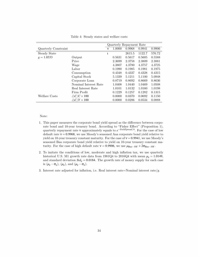
The results of welfare analysis are shown in the bottom rows of each panel of Table 4.Repayment rates are in quarterly frequency.
⟨Insert table 4 here⟩
Our estimate of the welfare cost of default is around 0.96% to 1.65% when g = 1.0149,which will be even higher if g = 1.024. While an estimate of roughly 1% of consumptionsounds small, at the consumption level of 2017Q2 it would amount to 118.397 billions ofchained 2009 dollars. Obviously this welfare loss due to default is non-negligible, comparingto the welfare cost of inflation estimated by Cooley and Hansen (1989) which is 0.52% ofthe consumption level when g = 1.024. This result emphasizes the important role of defaultin an economy.
As we can see, welfare costs increase with the severity of default in this artificial economy,which can also be confirmed by the results listed in panel 2 and 3 of Table 4. It canbe explained as follows: on the one hand, the decreased default penalty lowers marginalutility of consumption and thus pushes up consumption in optimal allocation; on the otherhand, firms will default more when they face loose regulation. According to “Fisher Effect”(Proposition 1), higher default rate requires higher risk premium which pushes up interestrate in corporate loan market. With higher financing cost, firms demand less corporate loanand thus reduce their investment and production, and it results in lower level of consumption.Higher marginal utility of consumption in turn pulls up default rate through “On-the-Verge
17
Conditions” (Proposition 3), which amplifies the effect of default penalty. In the end, thesecond effect dominates the first one.
Furthermore, it concludes that at the same default level, the cost of default is higherin the economy with higher money growth rate by comparing the results listed in penal 1,2 and 3 of Table 4. At the default level v = 0.9968, the welfare cost of default is 0.0244percentage of real output when expected inflation is low (g = 0.9965). When growth rate ofmoney supply is higher (g = 1.0149), the welfare cost correspondingly is increased to 0.0265percent of real output. Thus, the presence of default causes higher welfare loss at the samelevel of repayment rate when money growth rate is higher. When money growth rate ishigher, the nominal interest rate is higher at the same level of default rate.
It can be explained as follows. In “Fisher Effect” (Proposition 1), the change in inflationis greater than the change of real interest rate. Combining with the facts that more moneysupply pushes up price level and corporate loan is relatively constant, the level of con-sumption decreases (“On-the-Verge Conditions”, Proposition 3). Accordingly, with highermarginal utility of consumption, nominal interest rate in this economy increases, whichfurther press down consumption stream.
In section 6.1, cyclical properties show that at the same level of credit-regulation, whenmoney supply increases, the default rate will decreases. It explains why central bank injectedmoney into the economy during the financial crisis. But as discussed above, those policieslead the economy into financially more fragile regime which results in the greater loss ofsocial welfare with respect to the same level of default.
In this economy, markets are complete so each agent can completely hedge the risk.When firms are allowed to default, they face default penalties, causing social welfare loss.Detailed discussion abut social welfare analysis of default can be found in Dubey et al.(2000). According to their discussion, there are four drawbacks of the presence of default.First, creditors are less likely to lend when they rationally anticipating that they mightnot be paid. Second, borrowers may default on their promises regardless of their abilityto repay and contingencies that have been foreseen. Third, imposing default penalty is awelfare loss as it does not transfer social resources. Fourth, those agents who default imposean externality on those reliable agents who do not default. Due to information asymmetric,those agents who will fulfill their obligations cannot distinguish themselves from those whoare not reliable, and so reliable agents have to obtain the less favorable financing cost. Suchexternality problem can be modified by imposing penalties on defaulters (Akerlof, 1970).
But one thing needs to clarify here is that when the market is incomplete, it’s a totallydifferent story. According to Dubey et al. (2000), the social benefit of default option is likelyto outweigh social cost of default in incomplete market. To begin with, an individual agentwho decided to default at an optimal rate actually changes the given asset to a new one.Such a new asset is closer to his individual needs according to the benefit and cost causedby default. Moreover, it is a more desirable outcome in the perspective of the whole society.If individuals are not allowed to default, they only have the same given asset (fully repaytheir debts). But if there’s default option, each individual agent can change the given assetto a favorable on his idiosyncratic need. He/She can choose any repayment rate from 0 to1. Each agent can replace the given asset by a new one, thus one given asset is extended tomany. With a larger asset span, the social welfare is improved.
18
6.2.2 Welfare cost of default: short run effect
In order to estimate the short run welfare cost of default, we follow Lucas (1987) tocalculate the welfare cost of default as the gain from eliminating default. It is estimatedas the minimum percentage increase in the level of consumption in every period needed torender the agent indifferent between the economies with and without default.
We do 100 times simulations with 141 periods and take the mean as the welfare measures.The burn-up period is 100.
⟨Insert table 5 here⟩
As in the steady state, default causes social welfare loss. However, under the same levelof default regulation the sensitivity of default cost relative to the money growth rate is notsignificant. Thus, in the short run it may illude people that unconventional expansionarymonetary policies such as QE and Abenomics will not bring deterioration in terms of welfarecost of default. But as we showed in the long run effect, if these expansionary monetarypolicies last long, it actually leads to higher social welfare loss. The short run and long runeffects further confirm the propagation effect of the firm’s optimal repayment behaviour.
7 Concluding remarksIn sum, this paper employs an extended monetary “dynamic general equilibrium model”
(DSGE) with CIA constraints to analyze the impact of money and default on real economicactivities, especially default. It is the first attempt to clarify the role of endogenous discretedefault in infinite horizon CIA economy where positive response of output to monetaryshock holds. In addition, this study further estimates the welfare cost of default undervarious conditions based on this extended RBC model with CIA constraints and default.Finally, this paper studies the long-run effects of default on real business cycles by revealingsteady-state implications of this artificial economy.
Before welfare analysis, this study constructs non-pecuniary and non-linear defaultpenalty with certain parameters in a monetary DSGE model with CIA constraints to over-come the limitation of standard CIA models in generating positive relationship betweenoutput response and monetary shock. All the analysis in this paper is under the frameworkof the extended monetary DSGE model.
According to the quantitative analysis, endogenous default not only has significant in-fluence on the short-run economic fluctuations but also has long-run effects on the realeconomic activities. When default is considered as an equilibrium phenomena, the presenceof default alters the transmission mechanism of technology and monetary shock throughcredit market. The interest rate closely link the credit market with the real economic ac-tivities. On the one hand, the interest rate reflects the default risk premium in the creditmarket. When default rate is high, the interest rate is high due to high default risk premium(“Fisher Effect”, Proposition 1). And also, the interest rate itself will influence the defaultbehavior in this economy. On the other hand, the interest rate plays important role inreal economic activities because it reflects the financing cost of investment activities. Wheninterest rate is high, firms hesitate more to borrow money. Thus, in the economy withdefault, it generates financial accelerator effect due to interaction between financial frictionsand real economic activities. The presence of endogenous default amplifies and propagatesthe effects of shocks to real economy via credit market.
19
According to the welfare analysis, the default option induces social welfare loss. Thisstudy checks the welfare costs of default under different conditions and reveals that theamount of welfare cost induced by default varies with the levels of default rate and moneygrowth rate. First, the welfare cost of default increases with the severity of default. Whendefault rate is higher, the welfare cost caused by default is higher. Second, the welfare costof default increases with the money growth rate at a given level of default. In high inflationeconomy, given a certain repayment rate, the welfare cost of default is high. While in lowinflation economy, the welfare cost is low. Third, though the welfare cost of default is highin the long run, it is inconspicuous in the short run.
In the end, it is important to note the methodological limitations of the studies involvedin this thesis. First, most of parameters in this model are calibrated based on standardliterature and simple statistics of the U.S. historical data. The future research can useBayesian Estimation to adjust parameters based on the performance of the target economy.Second, to construct the monetary policy rule, it assumes a simple case where money growthrate in the steady state never changes, while in reality there are shifts in the steady state ofmoney growth rate corresponding to economic conditions. It’s more reasonable to investigatemore specific monetary policy rules such as the regime switching model. † Finally, this studymodels the cost of default as a reputation loss. With certain specific parameters of defaultpenalty, it can successfully generate hump-shaped positive response of output to positivemonetary shock. But the generalized methods to introduce default penalty is to be discussedin the future study.
†It would be perfectly possible to expand this exercise to include feedback rules in monetary policy, i.e.the nominal interest rate stipulated by the central bank via the money supply would positively respond tothe inflation and output gap. However, in this case, the growth rate of the money supply as monetary policyis modeled by an exogenous process whose log-linearized forms follow an AR(1) process, for examining theeffects of transitory monetary policy shocks.
20
ReferencesGeorge Akerlof. The market for “lemons”: Quality uncertainty and the market mechanism.
The quarterly journal of economics, pages 488–500, 1970.
Robert J Barro. The loan market, collateral, and rates of interest. Journal of money, Creditand banking, 8(4):439–456, 1976.
B Benanke and M Gertler. Agency costs, net worth, and business fluctuation. AER, 1989:14–31, 1989.
Ben Bernanke, Mark Gertler, and Simon Gilchrist. The financial accelerator in a quantitativebusiness cycle framework. Handbook of macroeconomics, 1:1341–1393, 1999.
Charles Carlstrom and Timothy Fuerst. Agency costs, net worth, and business fluctuations:A computable general equilibrium analysis. The American Economic Review, pages 893–910, 1997.
Lawrence Christiano, Roberto Motto, and Massimo Rostagno. The great depression and thefriedman-schwartz hypothesis. Technical report, National Bureau of Economic Research,2004.
Lawrence Christiano, Roberto Motto, and Massimo Rostagno. Financial factors in businesscycles. Mimeo, 2007.
Lawrence Christiano, Roberto Motto, and Massimo Rostagno. Shocks, structures or mon-etary policies? the euro area and us after 2001. Journal of Economic Dynamics andControl, 32(8):2476–2506, 2008.
Robert Clower. A reconsideration of the microfoundations of monetary theory. EconomicInquiry, 6(1):pp. 1–8, 1967.
Thomas Cooley and Gary Hansen. The inflation tax in a real business cycle model. TheAmerican Economic Review, pages 733–748, 1989.
Pradeep Dubey, John Geanakoplos, and Martin Shubik. Default in a general equilibriummodel with incomplete markets. Cowles Foundation for Research in Economics, 2000.
Pradeep Dubey, John Geanakoplos, and Martin Shubik. Default and punishment in generalequilibrium. econometrica, 73(1):1–37, 2005.
Jesús Fernández-Villaverde. The econometrics of dsge models. SERIEs, 1(1-2):3–49, 2010.
John Geanakoplos. Promises promises. The Economy as an Evolving Complex System II,eds, W. Brian Arthur, Steven Durlauf, and David Lane:285–320. Reading, MA: Addison–Wesley., 1997.
Andrea Gerali, Stefano Neri, Luca Sessa, and Federico Signoretti. Credit and banking ina dsge model of the euro area. Journal of Money, Credit and Banking, 42(s1):107–141,2010.
Charles Goodhart, Pojanart Sunirand, and Dimitrios Tsomocos. A model to analyse finan-cial fragility. Economic Theory, 27(1):107–142, 2006.
21
Gary Hansen. Indivisible labor and the business cycle. Journal of monetary Economics, 16(3):309–327, 1985.
Matteo Iacoviello. House prices, borrowing constraints, and monetary policy in the businesscycle. American economic review, pages 739–764, 2005.
Urban Jermann and Vincenzo Quadrini. Macroeconomic effects of financial shocks. Tech-nical report, National Bureau of Economic Research, 2009.
Nobuhiro Kiyotaki, John Moore, et al. Credit chains. Journal of Political Economy, 105(21):211–248, 1997.
Robert Lucas. Expectations and the neutrality of money. Journal of economic theory, 4(2):103–124, 1972.
Robert Lucas. Some international evidence on output-inflation tradeoffs. The AmericanEconomic Review, pages 326–334, 1973.
Robert Lucas. An equilibrium model of the business cycle. The Journal of Political Economy,pages 1113–1144, 1975.
Robert Lucas. Interest rates and currency prices in a two-country world. Journal of MonetaryEconomics, 10(3):335–359, 1982.
Robert Lucas and Nancy Stokey. Money and interest in a cash-in-advance economy. Econo-metrica, 55(3):491–513, 1987. ISSN 00129682.
James Nason and Timothy Cogley. Testing the implications of long-run neutrality for mone-tary business cycles. Journal of Applied Econometrics, 9:S37 – S70, 1994. ISSN 08837252.
Stephanie Schmitt-Grohé and Martın Uribe. Closing small open economy models. Journalof international Economics, 61(1):163–185, 2003.
F. Schorfheide. Loss function-based evaluation of dsge models. Journal of Applied Econo-metrics, 15(6):645–670, 2000.
Lloyd Shapley and Martin Shubik. Trade using one commodity as a means of payment. TheJournal of Political Economy, pages 937–968, 1977.
M Shubik and C Wilson. The optimal bankruptcy rule in a trading economy using fiatmoney. Journal of Economics, 37(3):337–354, 1977.
Martin Shubik. Commodity money, oligopoly, credit and bankruptcy in a general equilibriummodel. Economic Inquiry, 11(1):24–38, 1973.
D. Tsomocos. Equilibrium analysis, banking and financial instability. Journal of mathemat-ical economics, 39(5):619–655, 2003.
Dimitrios Tsomocos and Lea Zicchino. On modelling endogenous default. Discussion paper,548, 2005.
22
AppendicesAppendix A. List of detrended equations
Since money has stochastic trends and grows at a constant rate in the long run, theartificial economy is non-stationary. To begin with, all real variables qt = [Yt ,Ct , It ,Kt+1] andthe labor Nt are stationary because there is no technology or population growth. However,all nominal variables Qt = [Lt ,Wt ,Pt ] grow with the money supply Mt . Thus, all nominalvariables in the economy should be detrended to obtain a steady state. In detail, all thenominal variables should be divided by the money supply in this economy, i.e. Qt = Qt/Mt(Griffoli, 2007). The variables with hats represent stationary variables after detrending.Finally, the set of detrended equations of this model economy is listed as follows,
lnAt = ρA lnAt−1 +(1−ρA) ln A+σAεA,t
lngt = ρg lngt−1 +(1−ρg) ln g+σgεg,t
Et
(Pt
Ct+1Pt+1gt
)= Et
(βPt+1
Ct+2Pt+2gt+1
(α
Yt+1
Kt+1+(1−δ)
))Wt =
Lt
Nt
Lt
Nt=
ϕCt Pt
(1−ϕ)(1−Nt)(1−α) PtYt
Lt= Rt
1Rt
= βEt
(νtCt Pt
Ct+1Pt+1gt
)Ct +Kt+1 = (1−δ)Kt +Kα
t (AtNt)1−α
PtCt = gt
Yt = Kαt (AtNt)
1−α
Et
(1
Ct+1Pt+1gt
)= ι
[(1−νt)Rt Lt
]η
23
Appendix B. Basic CIA Economy without defaultThis part describes an basic CIA economy without default, which is the starting point
of the analysis in this paper. Default is not allowed in this economy and firms will pay backall their debts to households. There is no agency problem in this economy.
Optimization problem of households
Households solve the optimization problem as follows,
Firms in this economy face the optimization problem as follows,
max{Ft ,Kt+1,Nt ,Lt}
E0
∞
∑t=0
βt+1{
Ft
Ct+1Pt+1
}s.t.
WtNt ≤ Lt (19)
Ft = Lt +Pt
[Kα
t (AtNt)1−α −Kt+1 +(1−δ)Kt
]−WtNt −RtLt (20)
24
Appendix C. AR(1) process estimationIn this paper, external technology and monetary shocks are constructed as stochastic
AR(1) process. The AR(1) parameters are estimated from the time series data of thecalculated labor-augmenting technology factor and the money stock M1 for the U.S.
Money growth rate: In this model, the monetary policy follows stochastic AR(1) process,lngt = ρg lngt−1 +(1−ρg) ln g+σgεg,t (21)εg,t ∼ i.i.d. N(0,1)
where ρg represents smoothing coefficient of money supply growth rate, εg,t captures theunexpected monetary shock, and σg is the variance of the random shock.
To estimate AR(1) coefficient ρg and innovation variance σg , the money supply growthrate is calculated by divide the current period M1 by last period M1. Then take logarithmfor the M1 growth rate and run 1 lag auto-regression for log form of M1 growth rate.
According to the results of the AR(1) regression, the smoothing coefficient of moneysupply growth rate is ρg = 0.3522 and the variance of monetary shock is σg = 0.0168. Theunconditional mean of money growth rate is g = 1.0147.
Technology evolution process: In this model, the monetary policy follows stochastic AR(1)process,
where ρA represents smoothing coefficient of labor-augmenting technology factor, εA,tcaptures the unexpected technology shock, and σA is the variance of technology innovation.
To estimate AR(1) coefficient ρA and innovation variance σA , the labor-augmentingfactor data is derived from the “Cob supply growth rate is calculated by the “Cobb-Douglasproduction” function, Yt = Kα
t (AtNt)1−α, as follows,
ln(At) =ln(Yt)−α ln(Kt)
1−α− ln(Nt)
According to the results of the AR(1) regression, the smoothing coefficient of moneysupply growth rate is ρA = 0.8063 and the variance of monetary shock is σA = 0.0066. Thestationary technology is standardized to 1.
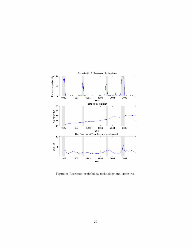
Figure 6: Recession probability, technology and credit risk
29
Tables
Table 1: Implied parameters
Description Parameter ValueOutput elasticity of capital α 0.3200Discount factor β 0.9900Consumption and leisure preference shifter ϕ 0.7730Depreciation rate δ 0.0250Coefficient of default penalty ι 150.00Elasticity of non-pecuniary default η 2.0000Steady state labor-augmenting technology factor A 1.0000Steady state money supply growth g 1.0147AR(1) coefficient of technology ρA 0.8063AR(1) coefficient of money supply growth ρg 0.3522Standard deviation of technology innovation σA 0.0066Standard deviation of monetary policy innovation σg 0.0168
30
Table 2: Statistics of U.S. and Artificial Economics
Standard Deviation Correlation(Percentage) with Output
U.S. time series Output 0.0168 1.0000Consumption 0.0091 0.8528Investment 0.0597 0.9109Capital Stock 0.0061 0.4195Hours 0.0177 0.8489Productivity 0.0112 0.0351CPI 0.0069 0.2608GNP Deflator 0.0046 0.2576
1. This paper measures the corporate bond yield spread as the difference between corpo-rate bond and 10-year treasury bond. According to “Fisher Effect” (Proposition 1),quarterly repayment rate ν approximately equals to e−YieldSpread/4. For the case of lowdefault rate ν = 0.9968, we use Moody’s seasoned Aaa corporate bond yield relative toyield on 10-year treasury constant maturity. For the case of ν= 0.9941, we use Moody’sseasoned Baa corporate bond yield relative to yield on 10-year treasury constant ma-turity. For the case of high default rate ν = 0.9906, we use µBaa−10Y +2σBaa−10Y .
2. To imitate the conditions of low, moderate and high inflation tax, we use quarterlyhistorical U.S. M1 growth rate data from 1981Q4 to 2016Q4 with mean µg = 1.0149,and standard deviation Stdg = 0.0184. The growth rate of money supply for each caseis (µg −σg), (µg), and (µg −σg).
3. Interest rate adjusted for inflation, i.e. Real interest rate=Nominal interest rate/g.