THE DESIGN AND CONTROL OF A BATTERY-SUPERCAPACITOR
HYBRID ENERGY STORAGE MODULE
FOR NAVAL APPLICATIONS
by
ISAAC J. COHEN
Presented to the Faculty of the Graduate School of
The University of Texas at Arlington in Partial Fulfillment
of the Requirements
for the Degree of
DOCTOR OF PHILOSOPHY
THE UNIVERSITY OF TEXAS AT ARLINGTON
May 2016
1
Acknowledgements
First and foremost I would like to thank my family for their support and encouragement
through my academic career. My wife, Bailey, my parents, Eli, Kelly, Cara, and Darryl,
and my siblings, Jesse and Brittany have all been sources of inspiration and a shelter
during stressful times.
I also want to thank my advisor, Dr. David Wetz, for not only his advice and mentorship
through this time, but also for his friendship. I would like to thank my mentors throughout
my academic career, Dr. Rasool Kenarangui, Dr. John Heinzel, and Dr. Qing Dong, for
all of their guidance and counsel. I would like to thank all of my committee members, Dr.
Wei-Jen Lee, Dr. William Dillon, and Dr. Ali Davoudi, for the invaluable suggestions and
comments that have helped me to shape my dissertation topic.
Finally, I would like to thank my lab mates over the years, Clint, Matt, Chris, Derek,
Caroline, Kendal, Calvin, Donald and Brian, for always offering a helping hand, allowing
me to bounce ideas off of you, and for telling me when those ideas were less than
intelligent.
Without all of your help and encouragement, none of this would have been possible and
for that, I thank all of you.
April 25, 2016
2
Abstract
THE DESIGN AND CONTROL OF A BATTERY-SUPERCAPACITOR HYBRID
ENERGY STORAGE MODULE FOR NAVAL APPLICATIONS
Isaac J. Cohen, PhD
The University of Texas at Arlington, 2016
Supervising Professor: David Wetz, PhD
As the Navy transitions to a more electrical fleet, the electrical architectures must
adapt to the changing load profiles. With the introduction of electrical propulsion and
new types of electrical energy based weapons, load profiles have become higher power
and more transient than ever seen before – especially during directed energy weapon
operation. One issue that has become apparent with the introduction of these transient
loads is the ability of traditional generation sources, such as fossil fuel generators, to
power them. Generators are stiff sources of power which suffer efficiency losses when
they deviate from operating at a constant maximum load. The logical answer to this
problem is to create a low-pass filter on the power flow by inserting an energy storage
device that is capable of both sinking and sourcing energy in order to keep the power
demand constant. In a Naval setting, the traditional approach to energy storage devices
would be lead acid batteries, but with recent developments in lithium-ion chemistries, it
would be preferable to utilize energy dense lithium-ion batteries to save precious space
and weight on board the ship. Although lithium-ion batteries offer many benefits, one
3
issue they face is a degradation of lifetime when the battery is cycled at high rates. One
solution that might come to mind is to simply use a power dense device that is relatively
unaffected by high rate usage such as a capacitor, but these devices typically do not
possess enough energy density to accommodate the system for long periods of time –
even sourcing power for periods of time where there may be a deficiency in generation.
One proposed method of overcoming these challenges is the integration of both energy
dense and power dense devices into a single module, referred to as a hybrid energy
storage module. In the case of a battery-supercapacitor hybrid energy storage module,
the voltage of each device is proportional to the energy stored. If these devices were
simply placed in parallel, as energy is drawn from the module, the voltage will drop on
the capacitor quicker than it will from the battery, leading to a situation where the battery
will source the majority of the current due to voltage dominance. In order to minimize
the current batteries, power electronic converters are placed in front of the battery to
actively control the amount of current flowing in and out of it. There are many
challenges when designing this type of system – especially when considering how to
integrate this into existing shipboard systems using commercial-off-the-shelf
components. The research presented here will delve into the design and control of a
hybrid energy storage module. The work presented here will present the mathematical
model of a hybrid energy storage module, it will show the simulation of this system
using the SimPowerSystems toolbox within MATLAB/Simulink, it will build this system
up on a tabletop testbed to validate the simulation results, and finally it will evaluate the
integration of this components using commercial-off-the-shelf components to mimic a
real-life implementation of such a system.
4
Table of Contents
Acknowledgements ......................................................................................................... 1
Abstract ........................................................................................................................... 2
List of Figures .................................................................................................................. 6
List of Tables ................................................................................................................. 10
Chapter 1: Introduction and Hypothesis ........................................................................ 11
Chapter 2: Mathematical Model of a HESM .................................................................. 19
Chapter 3: Simulink SimPowerSystems Model ............................................................. 34
Chapter 4: Tabletop HESM Experiment ........................................................................ 47
Chapter 5: COTS HESM Experiments .......................................................................... 60
DC Discharge Test ..................................................................................................... 60
DC Bi-Directional Test ............................................................................................... 64
AC Tests .................................................................................................................... 73
Generator Only Test ............................................................................................... 80
Generator with Recharge Test ................................................................................ 82
Generator and HESM Parallel Test ........................................................................ 86
Fuzzy Logic Control of COTS Equipment Test ....................................................... 90
Chapter 6: Summary and Conclusions .......................................................................... 98
Operation Manual for Controlling Xantrex XHR 33-33 for HESM Tabletop Tests .... 100
Operation Manual for HESM Tabletop Software ...................................................... 103
Operation Manual for COTS HESM Software .......................................................... 108
5
References .................................................................................................................. 112
Biographical Information .............................................................................................. 119
6
List of Figures
Figure 1: Circuit diagram of an example passive HESM [23] ........................................ 15
Figure 2: Circuit diagram of an example active HESM [20] ........................................... 15
Figure 3: Schematic of HESM for mathematical modeling ............................................ 20
Figure 4: Branch current designations for buck converter system ................................. 22
Figure 5: Branch current designations for boost converter system ............................... 27
Figure 6: Schematic of a generic battery/ultracapacitor HESM ..................................... 35
Figure 7: First input fuzzy membership function – the voltage of the output bus of the
HESM ............................................................................................................................ 38
Figure 8: Second input fuzzy membership function – the current flowing in or out of the
HESM ............................................................................................................................ 39
Figure 9: Output fuzzy membership function – the current direction and limit of the
battery ........................................................................................................................... 40
Figure 10: Fuzzy Logic Controller input vs. output relationship ..................................... 41
Figure 11: Block diagram of HESM experiment in SimPowerSystems toolbox ............. 42
Figure 12: Simulation results with if-then control ........................................................... 44
Figure 13: Simulation results using Fuzzy Logic Control ............................................... 45
Figure 14: Schematic of the Tabletop HESM ................................................................ 48
Figure 15: Photo of the tabletop setup .......................................................................... 52
Figure 16: Controller block diagram .............................................................................. 53
Figure 17: First input fuzzy membership function .......................................................... 55
Figure 18: Second input fuzzy membership function ..................................................... 55
Figure 19: Output fuzzy membership function ............................................................... 56
7
Figure 20: Surface plot depicting the fuzzy logic control inputs vs the output ............... 56
Figure 21 : Voltage Waveform of HESM Tabletop Experiment ..................................... 59
Figure 22: Current Waveforms of HESM Tabletop Experiment ..................................... 59
Figure 23: Hardware topology for DC discharge test of COTS devices......................... 61
Figure 24: COTS discharge only experimental setup for reproducing results achieved by
USC ............................................................................................................................... 62
Figure 25: Results from UTA experiment ...................................................................... 63
Figure 26: Results from USC experiment [24] ............................................................... 63
Figure 27: Experimental setup of the bi-directional test of a COTS HESM [25] ............ 67
Figure 28: Hardware topology for bi-directional DC test of COTS devices .................... 67
Figure 29: Overall current results from bi-directional test of a COTS HESM [25] .......... 71
Figure 30: Single pulse power results from DC bi-directional test of a COTS HESM [25]
...................................................................................................................................... 72
Figure 31: Hardware topology of the AC test of a COTS HESM [34] ............................ 75
Figure 32: Experimental setup of the AC test of a COTS HESM [34] ............................ 78
Figure 33: System power flow when only the generator is used to supply the load [34] 80
Figure 34: Fourier transform of power delivered to the load when only the generator is
used to supply the load [34] .......................................................................................... 81
Figure 35: RMS load voltage when only the generator is used to supply the load [34] . 82
Figure 36: System power flow when only the generator is used to supply the load and
the HESM loads the generator during recharge [34] ..................................................... 83
Figure 37: Fourier transform of power delivered to the load when only the generator is
used to supply the load and the HESM loads the generator during recharge [34] ........ 85
8
Figure 38: RMS load voltage when only the generator is used to supply the load and the
HESM loads the generator during recharge [34] ........................................................... 85
Figure 39: System power flow when the generator and HESM are simultaneously used
to supply the load and the HESM loads the generator during recharge [34] ................. 86
Figure 40: Fourier transform of power delivered to the load when the generator and
HESM are simultaneously used to supply the load and the HESM loads the generator
during recharge [34] ...................................................................................................... 88
Figure 41: RMS load voltage when the generator and HESM are simultaneously used to
supply the load and the HESM loads the generator during recharge [34] ..................... 88
Figure 42: Photo of Overall COTS HESM System ........................................................ 91
Figure 43: Close-up photo of the HESM ........................................................................ 92
Figure 44: Close-up of the NI Controller ........................................................................ 93
Figure 45: Bus voltage input membership function ....................................................... 94
Figure 46: HESM Current input membership function ................................................... 94
Figure 47: Battery Current output membership function ................................................ 95
Figure 48: Voltage plot from COTS HESM fuzzy logic control test ................................ 97
Figure 49: Current plot from COTS HESM fuzzy logic control test ................................ 97
Figure 50: VI of Xantrex XHR 33-33 GPIB Control ...................................................... 100
Figure 51: Simulink software for running the HESM tabletop ...................................... 103
Figure 52: PC104 target PC for HESM tabletop experiments ..................................... 104
Figure 53: PXI-QuickStart.vi Front Panel .................................................................... 108
Figure 54: RunLoadProfile.vi Front Panel ................................................................... 109
Figure 55: Main.vi Front Panel .................................................................................... 110
10
List of Tables
Table 1: Fuzzy Logic Rule-Base ................................................................................... 41
Table 2: Simulation values ............................................................................................ 43
Table 3: Numerical experimental results - comparison of if-then control with FLC ........ 45
Table 4: Fuzzy Logic Inputs and Outputs ...................................................................... 54
Table 5: Load Profile for HESM Tabletop Experiment ................................................... 57
Table 6: Load Profile for HESM Bi-Directional COTS Experiment ................................ 70
Table 7: Load Profile for HESM AC COTS Experiment ................................................. 78
Table 8: Numerical descriptions of membership functions ............................................ 95
Table 9: Load profile for the COTS HESM fuzzy logic control experiment .................... 96
11
Chapter 1: Introduction and Hypothesis
Traditionally, armed forces such as the United States Navy have relied upon fossil fuel
based energy generation to propel their ships and provide the electrical power needed
to operate their conventional and unique electrical loads, while weapon systems have
primarily relied on chemical combustion for propulsion and explosives to deliver damage
to the target. It is the near term desire of the US Navy to transition into a more electric
fleet, utilizing alternative forms of electrical energy generation to power both the
propulsion systems as well as a number of advanced electrical weapon systems
currently under development such as railguns, solid state lasers, and high power
microwave (HPM) generators, all of which rely on pulsed power sources [1, 2, 3]. With
this desire comes the need to integrate a large number of vastly different high power
electrical loads into a ship or forward operating base’s (FOBs) electrical generation grid.
Whether on a ship or on land, the power distribution grids being used are essentially
MicroGrids. These complex demands require that a number of different electrical
generation sources, such as fossil fuel generators, solar panels, fuel cells, flywheels,
wind turbines, batteries, and capacitors be installed and intelligently monitored and
controlled to ensure power delivery at all times to the critical loads. As one may expect,
this is not a trivial task.
The next generation naval destroyer, the Zumwalt class, is one example of the US
Navy’s shift towards implementing a more electric fleet. This class of ship features 78
MW of total distributed power generation as part of the next generation integrated power
systems (NGIPS). The NGIPS automatically adjusts power generation and distribution,
12
enabling future naval ships to more quickly adapt to changing combat conditions while
reliably engaging high power load systems [4, 5, 6, 7, 8].
Nearly all of the distributed generation sources discussed earlier are unregulated
sources which require the use of power electronic voltage converters, a point of
discussion later, to regulate their voltage before they are connected to a point of
common coupling. In islanded systems, such as on a naval vessel – where there is no
way to connect to a larger grid, the operation of high power loads can account for a
significant percentage of available power generation. As a result, they are capable of
forcing even fuel based power generation out of stiff operating conditions. To augment
the primary generation sources and maintain a stiff bus voltage, renewable energy
sources can be employed. These sources have trade-offs that must be properly
managed for success. Wind turbines and solar panels offer low power density and
intermittent operation, thereby reducing their usefulness and reliability as a direct form
of prime power generation for high continuous or pulsed power loads. Fuel cells offer
high energy density but low power density making them a bit more reliable but still not a
direct form of power generation in most cases. Flywheels offer a high combined power
and energy making them extremely useful for driving pulsed power systems, but their
cost and complexity often makes using them difficult [9, 10]. As will be shown later,
electrochemical batteries and capacitors, when used together, hold a great deal of
promise for use in driving pulsed power systems when combined together as batteries
are very energy dense and capacitors are power dense.
Historically, pulsed power research has been performed in large laboratories where size
and weight have not been the most pressing of concerns. Instead, the focus has been
13
on improving size, lifetime, reliability, and efficiency of high power switches,
intermediate energy storage systems, pulse forming lines and circuit topologies, and
new end use loads [11, 12, 13]. Before new advanced pulsed power systems, such as
those discussed earlier, can be implemented on either mobile or small footprint
stationary applications, the prime power source which drives them must be optimized
for both size and operational efficiency. While it would be ideal to have these loads
powered directly off of the same generation source used to propel the ship, the high
transient nature of the pulsed loads, coupled with the intermittent use of them, would
make the implementation of such a large generator extremely inefficient. This is where
alternative power sources, in particular electrochemical batteries and capacitors,
become vital for success.
Technological advancements in the field of electrochemistry have enabled the
development of batteries and capacitors with higher combined energy and power than
ever previously thought possible. Despite these advances, there is still no one cell
which possess the optimum power and energy density for all applications. Lithium-ion
batteries (LIBs) and electric-double-layer capacitors (EDLCs) with energy densities in
the range of 100 - 200 Wh/kg and 10 Wh/kg [14] respectively, are available
commercially off the shelf (COTS). COTS LIBs typically offer power densities in the
range of 0.1 – 0.5 kW/kg though specialty high power LIBs are available with power
densities as high as 28 kW/kg [15, 16, 17]. While these power densities, especially
those from the specialty cells, are very desirable, the usable capacity of the device can
often be significantly reduced when they are operated at their full power capabilities,
thereby reducing the operational efficiency and life span [18, 16, 19]. In addition to
14
these drawbacks, the expensive costs and commercial unavailability of many devices
causes them to be undesirable as the sole power source. Repetitive operation at high
power has been shown to significantly reduce a LIB’s cycle life, thereby increasing the
cost per ‘shot’ ratio of the system when more frequent battery replacement is required
[18]. While EDLCs do not offer high energy densities, they offer power densities as high
as 5 kW/kg and their long cycle life, up to 106 cycles, is not reduced when they are
operated at extreme power levels [20]. Therefore, the ability to utilize both of these
energy storage technologies within a single Hybrid Energy Storage Module (HESM)
provides the ability to optimize the power supply’s weight, volume, power density,
energy density, and cycle life.
The goal of the HESM is to maximize the operational and cycle life of the batteries by
limiting the currents which they discharge and recharge at. The capacitor is used to
supply the bulk of the transient currents and currents in excess of those which are
harmful to the battery. The battery is used as the main energy supply to recharge the
capacitor as well as supply a steady portion of the current to the load. Similarly, during
recharge the battery’s current can be limited while the capacitor absorbs a high rate of
recharge.
HESMs are not a new concept with the fundamental topologies having already been
developed, seen in Figure 1 and Figure 2. In its simplest form, the passive topology,
batteries and capacitors are simply connected in parallel with their load. In Figure 1, the
load is a two-quadrant DC/DC converter and a DC bus. In this configuration, the internal
equivalent series resistance (ESR) of each device drives where the energy supplied to
the load comes from. In the case of high transient loads, the capacitors lower ESR
15
enables them to supply the front end power while the batteries are used to supply the
steady energy [21]. [22] previously showed that the front end and steady state power
draw supplied by batteries is significantly reduced when capacitors are added.
Figure 1: Circuit diagram of an example passive HESM [23]
Figure 2: Circuit diagram of an example active HESM [20]
An active HESM topology is more complex, but this comes with increased
instantaneous power capabilities and longevity. With this topology, the focus is on
maintaining the system bus voltage and controlling the currents drawn out of the
distributed power sources. Notice in Figure 2 how the battery is independently regulated
16
using a boost converter. The output of the boost converter feeds the capacitor and then
the DC/DC converter, therefore the capacitor picks up whatever portion of the load is
not supplied by the battery.
Previous work has shown that Hybrid Energy Storage Modules (HESMs) can contribute
to not only improve the performance of an energy storage device (ESD), but also
overcome the limitations of the individual components of the architecture, such as the
power delivery limitations of a battery or the energy storage limitations of an
ultracapacitor [24, 25, 26]. While this topology has been verified, there are still some
questions on how to best control them. Many of the published efforts thus far have
focused on the development of control algorithms and mathematical models for
specialized, research based, reconfigurable power electronic converters. In these
cases, validations of the experimental control algorithms have been performed using
small proof of concept hardware setups. Voltages and currents are typically in the
vicinity of a few volts or amps, respectively, allowing the power electronic converter to
be the focus of the work. While the previously published works do a great job at
demonstrating the many advantages a HESM offers, significant time, effort, and money
is required to build up the capability to develop custom power electronics. This can be
prohibitive to the advancement of HESM research outside of the power electronics area.
[27] designed a low cost digital energy management system and an optimal control
algorithm was developed in [28] to coordinate slow ESDs and fast ESDs. While these
control developments have been very useful, they do not address the need for a
controller that is capable of interfacing with COTS products. Fuzzy logic control has
been used in many applications such as [29], who developed an intuitive fuzzy logic
17
based learning algorithm which was implemented to reduce intensive computation of a
complex dynamics such as a humanoid. Some, such as [30] have utilized fuzzy logic
control to drive a HESM, but in their case, they used the controller in order to eliminate
the need to constantly calculate resource intensive Riccati equations to assist in
choosing gains for an adaptive Linear-Quadratic Regulator controller. Others, such as
[31, 32] developed an energy-based split and power sharing control strategy for hybrid
energy storage systems, but these strategies are focused on different target variables
such as loss reduction, leveling the components state of charge, or optimizing system
operating points in a vehicular system.
When constructing a HESM for naval pulsed power load applications, several design
parameters must be considered to develop the controller. First, the HESM must be
responsible for supplying all load demands that it might encounter. Energy sizing
techniques such as shown in [33] should be applied in order to assist in meeting this
demand. Second, the HESM should add the benefit of becoming an additional source
during parallel operation with an existing shipboard power system, offering a reduction
in external power system sizing. Finally, the HESM should operate as a power buffer
during this parallel operation, offering improved power quality to the load from sluggish
generation sources, such as fossil-fuel generators, such as seen in [34].
There are many combinations of high power density and high energy density ESDs that
can be used to create a HESM, but a common topology that will be evaluated in this
paper is the combination of ultracapacitors and batteries. Although the Navy has
traditionally used lead-acid batteries as the go-to ESD, lithium-ion batteries (LIBs) offer
a higher energy and power density with respect to both volume and weight. In this
18
scenario, a HESM becomes even more necessary as previous research has shown that
while LIBs are capable of being cycled at high rates, they degrade much more quickly
[34] – necessitating the limiting of power to and from the battery to be as minimal as
possible. This limitation can be implemented through the introduction of intelligent
controls.
In the work presented here, an active HESM will be designed and developed using
COTS components. A challenge that will be presented by this system is how to offer a
form of system level control over the integrated components. To achieve this, steps will
be taken to mathematically model a HESM, design a controller, model and simulate the
controller, use the controller on a custom tabletop testbed implementation of a HESM,
and finally implement the controller on a real COTS integrated system. It is
hypothesized in this work that a system level control can be achieved to satisfy the
requirements of an equivalent energy storage device in a pulsed power naval setting
while offering the previously mentioned advantages that a HESM contributes. The result
of this work is a testbed, which can be utilized to easily evaluate different energy
storage chemistries and power system integration techniques.
19
Chapter 2: Mathematical Model of a HESM
The first step to developing a controller for the system is to mathematically model it.
Other researchers have spent time modeling this system mathematically such as [35],
which presented a detailed small-signal mathematical model that represents the
dynamics of the converter interfaced energy storage system around a steady-state
operating point. Their model considered the variations in the battery current,
supercapacitor current, and DC load bus voltage as the state variables, the variations in
the power converter’s duty cycle as the input, and the variations in the battery voltage,
supercapacitor voltage, and load current as external disturbances. Modeling this system
mathematically can be difficult for a multitude of reasons. Considerations must be made
with regards to the level of detail to include in the model and degree of linearizing
applied to the system. In the case of a HESM there is the additional problem of properly
representing the energy storage devices. Typically, when power electronics converters
are mathematically described in an entry level course, they utilize an ideal voltage
source as an input and a common resistor as a load, but with a HESM, energy storage
devices serve as both the source and the load and exhibit bi-directional power flow.
Alone, the system can be considered passive, but with the addition of power generation,
there are still opportunities to cause enormous instabilities. Approaching this system
mathematically, the ultracapacitor is simple to model in the idea that it is simply a
capacitor with a large capacitance and an equivalent series resistance, so it offers no
challenge in modeling, but the model of a battery is different. To make it simple for both
model description and for controller design, it was decided that the battery model to use
would be Saft’s RC model of a lithium-ion battery [36]. In this model, they use a bulk
20
capacitor to describe the large energy storage of the device and they use a few
resistors to model the ESR and chemical impedances along with a second capacitor to
emulate surface capacitance of the terminals. The HESM schematic that will be used to
mathematically model the system can be seen in Figure 3.
Figure 3: Schematic of HESM for mathematical modeling
Where,
Cb Bulk Capacitance S2 Boost Converter Switch Cc Surface Capacitance L Power Inductor Re Electrochemical Resistance RL ESR of Inductor Rc Double Layer Resistance Cu Ultracapacitor Rt Terminal Resistance Ru ESR of Ultracapacitor S1 Buck Converter Switch ζ Load and/or Generation Disturbance
Since there are two switches that can have binary states, this system is considered time
varying. The sets of equations that describe the system in each of the binary states are
shown below, splitting up into the different states of the system, based on the directions
of power flow of the system and the state of the switches.
21
In the equations shown below, the states are defined as:
[
1
2
3
4
] = [
𝑖𝐿𝑉𝑢
𝑉𝑏
𝑉𝑐
] ( 1 )
There are essentially two systems to consider when mathematically describing this
HESM. The first system is the buck converter system, where power flows from the
battery to the ultracapacitor. The second system is the boost converter system, where
the power flows from the ultracapacitor to the battery. These systems are used
separately and exist separately and therefore will be analyzed separately with different
designations for current flow and voltage polarities. The branch currents designated in
the buck converter system can be seen in Figure 4 and the designations made for the
boost converter system can be seen in Figure 5. Analysis will begin with analyzing the
power flow from the battery to the ultracapacitor and will then be followed with analyzing
the power flow from the ultracapacitor to the battery. MOSFET switches are considered
ideal in this analysis and therefore are assumed to have no voltage drop during
conduction. The body diodes of the MOSFETs are also considered to be ideal and
therefore will be assumed to have no forward breakdown voltage, no voltage drop
during conduction, and infinite reverse breakdown voltage.
22
Figure 4: Branch current designations for buck converter system
State 1: The power flows from the battery to the ultracapacitor; S1 is on and S2 is off
𝑉𝑐 + 𝑅𝑐𝑖𝑐 + 𝑅𝑡𝑖𝐿 + 𝑉𝐿 + 𝑅𝐿𝑖𝐿 + 𝑅𝑢𝑖𝑢 + 𝑉𝑢 = 0 ( 2 )
→ 1(𝐿) + 2(𝑅𝑢𝐶𝑢) + 4(𝑅𝑐𝐶𝑐) = 𝑥1(−𝑅𝐿 − 𝑅𝑡) − 𝑥2 − 𝑥4 ( 3 )
𝑖𝐿 − 𝑖𝑢 − 𝜁 = 0 ( 4 )
→ 2(−𝐶𝑢) = −𝑥1 + 𝜁 ( 5 )
𝑉𝑏 + 𝑅𝑒𝑖𝑏 − 𝑅𝑐𝑖𝑐 − 𝑉𝑐 = 0 ( 6 )
→ 3(𝑅𝑒𝐶𝑏) + 4(−𝑅𝑐𝐶𝑐) = −𝑥3 + 𝑥4 ( 7 )
𝑖𝑏 + 𝑖𝑐 − 𝑖𝐿 = 0 ( 8 )
→ 3(𝐶𝑏) + 4(𝐶𝑐) = 𝑥1 ( 9 )
These equations are in the form 𝑀 = 𝐴𝑥 + 𝐹𝜁. Where,
𝑀1 = [
𝐿 𝑅𝑢𝐶𝑢 0 𝑅𝑐𝐶𝑐
0 −𝐶𝑢 0 00 0 𝑅𝑒𝐶𝑏 −𝑅𝑐𝐶𝑐
0 0 𝐶𝑏 𝐶𝑐
] ( 10 )
𝐴1 = [
−𝑅𝐿 − 𝑅𝑡 −1 0 −1−1 0 0 00 0 −1 11 0 0 0
] ( 11 )
23
𝐹1 = [
0100
] ( 12 )
1 ≡ 𝑀1−1𝐴1
=
[ (
𝑅𝑒2
𝑅𝑐 + 𝑅𝑒− 𝑅𝑒 − 𝑅𝐿 − 𝑅𝑡 − 𝑅𝑢)
𝐿
−1
𝐿
−𝑅𝑐
𝐿(𝑅𝑐 + 𝑅𝑒)
−𝑅𝑒
𝐿(𝑅𝑐 + 𝑅𝑒)1
𝐶𝑈𝐶0 0 0
(1 −𝑅𝑒
(𝑅𝑐 + 𝑅𝑒))
𝐶𝑏0
−1
𝐶𝑏(𝑅𝑐 + 𝑅𝑒)
1
𝐶𝑏(𝑅𝑐 + 𝑅𝑒)𝑅𝑒
𝐶𝑐(𝑅𝑐 + 𝑅𝑒)0
1
𝐶𝑐(𝑅𝑐 + 𝑅𝑒)
−1
𝐶𝑐(𝑅𝑐 + 𝑅𝑒)]
( 13 )
1 ≡ 𝑀1−1𝐹1 =
[ 𝑅𝑢
𝐿−1
𝐶𝑢
00 ]
( 14 )
This mathematical model describes the relationship of the states of the system when
the switch of the “buck converter” is switched closed. To see the relationships of the
system while the switch is open, State 2 is considered.
State 2: The power flows from the battery to the ultracapacitor; S1 is off and S2 is off
𝑉𝐿 + 𝑅𝐿𝑖𝐿 + 𝑅𝑢𝑖𝑢 + 𝑉𝑢 = 0 ( 15 )
→ 1(𝐿) + 2(𝑅𝑢𝐶𝑢) = 𝑥1(−𝑅𝐿) − 𝑥2 ( 16 )
𝑖𝐿 − 𝑖𝑢 − 𝜁 = 0 ( 17 )
→ 2(−𝐶𝑢) = −𝑥1 + 𝜁 ( 18 )
𝑉𝑏 + 𝑅𝑒𝑖𝑏 − 𝑅𝑐𝑖𝑐 − 𝑉𝑐 = 0 ( 19 )
→ 3(𝑅𝑒𝐶𝑏) + 4(−𝑅𝑐𝐶𝑐) = −𝑥3 + 𝑥4 ( 20 )
24
𝑖𝑏 + 𝑖𝑐 = 0 ( 21 )
→ 3(𝐶𝑏) + 4(𝐶𝑐) = 0 ( 22 )
These equations are in the form 𝑀 = 𝐴𝑥 + 𝐹𝜁. Where,
𝑀2 = [
𝐿 𝑅𝑢𝐶𝑢 0 00 −𝐶𝑢 0 00 0 𝑅𝑒𝐶𝑏 −𝑅𝑐𝐶𝑐
0 0 𝐶𝑏 𝐶𝑐
] ( 23 )
𝐴2 = [
−𝑅𝐿 − 𝑅𝑡 −1 0 0−1 0 0 00 0 −1 10 0 0 0
] ( 24 )
𝐹2 = [
0100
] ( 25 )
2 ≡ 𝑀2−1𝐴2 =
[ (−𝑅𝐿 − 𝑅𝑢)
𝐿
−1
𝐿0 0
1
𝐶𝑢0 0 0
0 0−1
𝐶𝑏(𝑅𝑐 + 𝑅𝑒)
1
𝐶𝑏(𝑅𝑐 + 𝑅𝑒)
0 01
𝐶𝑐(𝑅𝑐 + 𝑅𝑒)
−1
𝐶𝑐(𝑅𝑐 + 𝑅𝑒)]
( 26 )
2 ≡ 𝑀2−1𝐹2 =
[
𝑅𝑢
𝐿
−1
𝐶𝑢
00 ]
( 27 )
To calculate the outputs, there are only really two values that are of any concern in this
system during this power flow direction. In this case, only the DC bus voltage and the
inductor current are of interest.
25
These values can be found with the equations,
𝑦 = 𝑅𝑢𝑖𝑢 + 𝑉𝑢 ( 28 )
→ 𝑅𝑢𝐶𝑢2 + 𝑥2 ( 29 )
From equation 5,
2 =𝑥1
𝐶𝑢−
𝜁
𝐶𝑢 ( 30 )
𝑦 = 𝑅𝑢𝑥1 + 𝑥2 − 𝑅𝑢𝜁 ( 31 )
This output is arranged in the format of 𝑦 = 𝐶𝑥 + 𝐺𝜁 where,
𝐶1,2 = [𝑅𝑢 1 0 01 0 0 0
] ( 32 )
𝐺1,2 = [
0−𝑅𝑢
00
] ( 33 )
Since this system is binary in nature and literally changes the plant during each state, it
can be represented as an average between these two states where the averaging
number is determined by the percentage of time during a cycle spent in each state.
Since these switches are driven by pulsed width modulation, the duty cycle of this signal
can be considered the percentage of time in a period that each state exists inside.
Another note is that there is no controllable input to this system besides the duty cycle
of each switch. This is an interesting problem to overcome and is a suggested topic of
research for future work.
26
For now, the combination of these two states for power flowing from the battery towards
the ultracapacitor can be described by the equations:
= (𝑑1 + (1 − 𝑑)2)𝑥 + 𝐹𝜁 ( 34 )
→ = (𝑑1𝑥 + 2𝑥 − 𝑑2𝑥) + 𝐹𝜁 ( 35 )
→ = (2𝑥 + 𝑑(1 − 2)𝑥) + 𝐹𝜁 ( 36 )
1 − 2 =
[ (
𝑅𝑒2
𝑅𝑐 + 𝑅𝑒− 𝑅𝑒 − 𝑅𝑡)
𝐿0 −
𝑅𝑐
𝐿(𝑅𝑐 + 𝑅𝑒)−
𝑅𝑒
𝐿(𝑅𝑐 + 𝑅𝑒)
0 0 0 0
(1 −𝑅𝑒
(𝑅𝑐 + 𝑅𝑒))
𝐶𝑏0 0 0
𝑅𝑒
𝐶𝑐(𝑅𝑐 + 𝑅𝑒)0 0 0
]
( 37 )
The next two states describe the system when power flows from the ultracapacitor to
the battery, in other words the boost converter system. Keeping this in mind, the branch
current designations change, as seen in Figure 5.
27
Figure 5: Branch current designations for boost converter system
State 3: The power flows from the ultracapacitor to the battery; S1 is off and S2 is on
𝑉𝑢 + 𝑅𝑢𝑖𝑢 + 𝑅𝐿𝑖𝐿 + 𝑉𝐿 = 0 ( 38 )
→ 1(𝐿) + 2(𝑅𝑢𝐶𝑢) = 𝑥1(−𝑅𝐿) − 𝑥2 ( 39 )
−𝑖𝐿 + 𝑖𝑢 + 𝜁 = 0 ( 40 )
→ 2(𝐶𝑢) = 𝑥1 − 𝜁 ( 41 )
−𝑉𝑐 − 𝑅𝑐𝑖𝑐 + 𝑅𝑒𝑖𝑏 + 𝑉𝑏 = 0 ( 42 )
→ 3(𝑅𝑒𝐶𝑏) + 4(−𝑅𝑐𝐶𝑐) = −𝑥3 + 𝑥4 ( 43 )
−𝑖𝑏 − 𝑖𝑐 = 0 ( 44 )
→ 3(−𝐶𝑏) + 4(−𝐶𝑐) = 0 ( 45 )
These equations are in the form 𝑀 = 𝐴𝑥 + 𝐹𝜁. Where,
28
𝑀3 = [
𝐿 𝑅𝑢𝐶𝑢 0 𝑅𝑐𝐶𝑐
0 𝐶𝑢 0 00 0 𝑅𝑒𝐶𝑏 −𝑅𝑐𝐶𝑐
0 0 −𝐶𝑏 −𝐶𝑐
] ( 46 )
𝐴3 = [
−𝑅𝐿 −1 0 01 0 0 00 0 −1 10 0 0 0
] ( 47 )
𝐹3 = [
0−100
] ( 48 )
3 ≡ 𝑀3−1𝐴3 =
[ (−𝑅𝐿 − 𝑅𝑢)
𝐿−
1
𝐿0 0
−1
𝐶𝑢0 0 0
0 0−1
𝐶𝑏(𝑅𝑐 + 𝑅𝑒)
1
𝐶𝑏(𝑅𝑐 + 𝑅𝑒)
0 01
𝐶𝑐(𝑅𝑐 + 𝑅𝑒)
−1
𝐶𝑐(𝑅𝑐 + 𝑅𝑒)]
( 49 )
3 ≡ 𝑀3−1𝐹3 =
[
𝑅𝑢
𝐿
−1
𝐶𝑢
00 ]
3 ≡ 𝑀3−1𝐹3 =
[
𝑅𝑢
𝐿
−1
𝐶𝑢
00 ]
( 50 )
This mathematical model describes the relationship of the states of the system when
the switch of the “boost converter” is switched closed. To see the relationships of the
system while the switch is open, State 4 is considered.
29
State 4: The power flows from the ultracapacitor to the battery; S1 is off and S2 is off
𝑉𝑐 + 𝑅𝑐𝑖𝑐 + 𝑅𝑡𝑖𝐿 + 𝑉𝐿 + 𝑅𝐿𝑖𝐿 + 𝑅𝑢𝑖𝑢 + 𝑉𝑢 = 0 ( 51 )
→ 1(𝐿) + 2(𝑅𝑢𝐶𝑢) + 4(𝑅𝑐𝐶𝑐) = 𝑥1(−𝑅𝐿 − 𝑅𝑡) − 𝑥2 − 𝑥4 ( 52 )
−𝑖𝐿 + 𝑖𝑢 + 𝜁 = 0 ( 53 )
→ 2(𝐶𝑢) = 𝑥1 − 𝜁 ( 54 )
𝑉𝑏 + 𝑅𝑒𝑖𝑏 − 𝑅𝑐𝑖𝑐 − 𝑉𝑐 = 0 ( 55 )
→ 3(𝑅𝑒𝐶𝑏) + 4(−𝑅𝑐𝐶𝑐) = −𝑥3 + 𝑥4 ( 56 )
−𝑖𝑏 − 𝑖𝑐 + 𝑖𝐿 = 0 ( 57 )
→ 3(−𝐶𝑏) + 4(−𝐶𝑐) = −𝑥1 ( 58 )
These equations are in the form 𝑀 = 𝐴𝑥 + 𝐹𝜁. Where,
𝑀4 = [
𝐿 𝑅𝑢𝐶𝑢 0 𝑅𝑐𝐶𝑐
0 𝐶𝑢 0 00 0 𝑅𝑒𝐶𝑏 −𝑅𝑐𝐶𝑐
0 0 −𝐶𝑏 −𝐶𝑐
] ( 59 )
𝐴4 = [
−𝑅𝐿 − 𝑅𝑡 −1 0 −11 0 0 00 0 −1 1
−1 0 0 0
] ( 60 )
𝐹4 = [
0−100
] ( 61 )
4 ≡ 𝑀4−1𝐴4 =
[ (
𝑅𝑒2
𝑅𝑐 + 𝑅𝑒− 𝑅𝑒 − 𝑅𝑡 − 𝑅𝑢)
𝐿
−1
𝐿
−𝑅𝑐
𝐿(𝑅𝑐 + 𝑅𝑒)
−𝑅𝑒
𝐿(𝑅𝑐 + 𝑅𝑒)1
𝐶𝑢0 0 0
(1 −𝑅𝑒
(𝑅𝑐 + 𝑅𝑒))
𝐶𝑏0
−1
𝐶𝑏(𝑅𝑐 + 𝑅𝑒)
1
𝐶𝑏(𝑅𝑐 + 𝑅𝑒)𝑅𝑒
𝐶𝑐(𝑅𝑐 + 𝑅𝑒)0
1
𝐶𝑐(𝑅𝑐 + 𝑅𝑒)
−1
𝐶𝑐(𝑅𝑐 + 𝑅𝑒)]
( 62 )
30
4 ≡ 𝑀2−1𝐹2 =
[ 𝑅𝑢
𝐿−1
𝐶𝑢
00 ]
( 63 )
To calculate the outputs, a similar approach is taken to the previous power flow
direction “system”. In this case, only the battery bus voltage and the inductor current are
of interest. The main difference in this case is that the battery voltage changes based
not only on the states of the system, but whether or not the battery is “conducting”. This
is due to the ESR drop dictated by Rt. During state 3, where the battery is not
conducting, the output is defined as,
𝑦 = 𝑅𝑐𝑖𝑐 + 𝑉𝑢 ( 64 )
→ 𝑅𝑐𝐶𝑐4 + 𝑥4 ( 65 )
From equation 43 and 45,
4 =−3𝐶𝑏
𝐶𝑐 ( 66 )
3 = −𝑥3
𝑅𝑒𝐶𝑏+
𝑥4
𝑅𝑒𝐶𝑏+
4𝑅𝑐𝐶𝑐
𝑅𝑒𝐶𝑏 ( 67 )
These equations can be rearranged to obtain,
4 =𝑥3 − 𝑥4
𝐶𝑐(𝑅𝑒 + 𝑅𝑐) ( 68 )
𝑦 =𝑅𝑐𝑥3
𝑅𝑒 + 𝑅𝑐−
𝑅𝑐𝑥4
𝑅𝑒 + 𝑅𝑐+ 𝑥4 ( 69 )
31
This output is arranged in the format of 𝑦 = 𝐶𝑥 + 𝐺𝜁 where,
𝐶3 = [0 0
𝑅𝑐
𝑅𝑒 + 𝑅𝑐1 +
𝑅𝑐
𝑅𝑒 + 𝑅𝑐
1 0 0 0
] ( 70 )
𝐺3 = 0 ( 71 )
This describes the battery bus and the inductor current while the battery is conducting in
a recharge state. To define the system during a non-conducting time the equations are,
𝑦 = 𝑅𝑡𝑖𝐿 + 𝑅𝑐𝑖𝑐 + 𝑉𝑢 ( 72 )
→ 𝑅𝑡𝑥1 + 𝑅𝑐𝐶𝑐4 + 𝑥4 ( 73 )
From equation 56 and 58,
4 =𝑥1
𝐶𝑐−
3𝐶𝑏
𝐶𝑐 ( 74 )
3 = −𝑥3
𝑅𝑒𝐶𝑏+
𝑥4
𝑅𝑒𝐶𝑏+
4𝑅𝑐𝐶𝑐
𝑅𝑒𝐶𝑏 ( 75 )
These equations can be rearranged to obtain,
4 =𝑅𝑒𝑥1 + 𝑥3 − 𝑥4
𝑅𝑒𝐶𝑐 + 𝑅𝑐𝐶𝑐 ( 76 )
𝑦 = 𝑥1 (𝑅𝑡 +𝑅𝑒𝑅𝑐
𝑅𝑒 + 𝑅𝑐) + 𝑥3 (
𝑅𝑐
𝑅𝑒 + 𝑅𝑐) + 𝑥4 (1 +
𝑅𝑐
𝑅𝑒 + 𝑅𝑐) ( 77 )
32
This output is arranged in the format of 𝑦 = 𝐶𝑥 + 𝐺𝜁 where,
𝐶4 = [𝑅𝑡 +
𝑅𝑒𝑅𝑐
𝑅𝑒 + 𝑅𝑐0
𝑅𝑐
𝑅𝑒 + 𝑅𝑐1 +
𝑅𝑐
𝑅𝑒 + 𝑅𝑐
1 0 0 0
] ( 78 )
𝐺4 = 0 ( 79 )
Again, this system is binary in nature and can be represented as an average between
these two states where the averaging number is determined by the percentage of time
during a cycle spent in each state. The combination of these two states for power
flowing from the ultracapacitor towards the battery can be described by the equations:
= (𝑑3 + (1 − 𝑑)4)𝑥 + 𝐹𝜁 ( 80 )
→ = (𝑑3𝑥 + 4𝑥 − 𝑑4𝑥) + 𝐹𝜁 ( 81 )
→ = (3𝑥 + 𝑑(3 − 4)𝑥) + 𝐹𝜁 ( 82 )
3 − 4 =
[ (
−𝑅𝑒2
𝑅𝑐 + 𝑅𝑒+ 𝑅𝑒 + 𝑅𝐿(−𝑅𝑡 − 1))
𝐿0
𝑅𝑐
𝐿(𝑅𝑐 + 𝑅𝑒)
𝑅𝑒
𝐿(𝑅𝑐 + 𝑅𝑒)−2
𝐶𝑢0 0 0
(𝑅𝑒
(𝑅𝑐 + 𝑅𝑒)− 1)
𝐶𝑏0 0 0
−𝑅𝑒
𝐶𝑐(𝑅𝑐 + 𝑅𝑒)0 0 0
]
( 83 )
Although it is fairly straight forward to mathematically describe this system in its
separate states, it is very difficult to design a controller for this system given its non-
linear and time varying qualities. There are many advanced methods of control that
have been developed to achieve control of these types of converters such as
backstepping control, slide mode control, or optimal control techniques such as the
Pontryagin’s Minimum Principle, but since it is intended to eventually transition the
33
controller design to a COTS system whose internals are either unknown or difficult to
obtain, for the purposes of the work presented here, it does not make sense to spend
time with these advanced control concepts when the time averaged model works just
fine with using a simple PI controller. Although this mathematical approach has given
insight to the system and provided a glimpse into the dynamics, it was decided at this
point to move forward with a circuit simulator such as Simulink’s SimPowerSystems,
which offers more dynamic electronic component models and a more robust
environment for implementing the desired system level controls that will be eventually
implemented on top of a COTS system.
34
Chapter 3: Simulink SimPowerSystems Model
While this work aims to address the need for a system level control for COTS devices,
in order to simulate the controller in MATLAB/Simulink, it is necessary to use a
simplified model of a HESM and its power converters. In the material below,
MATLAB/Simulink’s SimPowerSystems toolbox will be utilized instead of a
mathematical model.
A generic schematic of a HESM is shown in Figure 6. In this schematic, a simple buck-
boost converter is utilized in order to give the controller a method of bi-directional
voltage and current control. The load and the generator are tied together as one
variable current source/sink as the system which the HESM augments can be seen as a
generalized external power disturbance. When mathematically modeling this system, in
similar fashion to [35], C1 and C2, the output capacitors for each direction of power
flow, hold the state variables of the battery bus voltage and the DC load bus voltage and
L, the power inductor, holds the state variable of the power converter current, and the
combined current sourcing or sinking from the load and generation is the external
disturbance, denoted as ζ. For instance, when ζ > 0, the generator is producing more
current than the load is drawing, but when ζ < 0, the load is drawing more current than
the generation is producing. There are multiple equations to describe this circuit during
operation, based on the state of the switches. To demonstrate the variation of this
system over time, the mathematical equations that represent these states are shown
below. For simplicity, the system will be evaluated in each direction of power flow while
treating the load ESD as an omitted independent variable, shown in the circuit as V1
and V2.
35
Figure 6: Schematic of a generic battery/ultracapacitor HESM
1. State 1: When power flows from the battery towards the ultracapacitor and when
S1 is on and S2 is off,
𝐿𝑑𝑖𝐿𝑑𝑡
= 𝑉𝐶1 − 𝑉𝐶2 ( 84 )
𝐶1
𝑑𝑉𝐶1
𝑑𝑡= 𝑖𝐿 − 𝑖𝑉1 ( 85 )
𝐶2
𝑑𝑉𝐶2
𝑑𝑡= 𝑖𝐿 − 𝑖𝑉2 − 𝜁
( 86 )
2. State 2: When power flows from the battery towards the ultracapacitor and when
S1 is off and S2 is off,
𝐿𝑑𝑖𝐿𝑑𝑡
= −𝑉𝐶2 ( 87 )
𝐶1
𝑑𝑉𝐶1
𝑑𝑡= −𝑖𝑉1 ( 88 )
𝐶2
𝑑𝑉𝐶2
𝑑𝑡= 𝑖𝐿 − 𝑖𝑉2 − 𝜁
( 89 )
36
3. State 3: When power flows from the ultracapacitor towards the battery and when
S1 is off and S2 is on,
𝐿𝑑𝑖𝐿𝑑𝑡
= 𝑉𝐶2 ( 90 )
𝐶1
𝑑𝑉𝐶1
𝑑𝑡= −𝑖𝑉1 ( 91 )
𝐶2
𝑑𝑉𝐶2
𝑑𝑡= 𝑖𝑉2 − 𝑖𝐿 − 𝜁
( 92 )
4. State 4: When power flows from the ultracapacitor towards the battery and when
S1 is off and S2 is off,
𝐿𝑑𝑖𝐿𝑑𝑡
= 𝑉𝐶2 − 𝑉𝐶1 ( 93 )
𝐶1
𝑑𝑉𝐶1
𝑑𝑡= 𝑖𝐿 − 𝑖𝑉1 ( 94 )
𝐶2
𝑑𝑉𝐶2
𝑑𝑡= 𝑖𝑉2 − 𝑖𝐿 − 𝜁
( 95 )
These mathematical equations are presented here to reinforce the idea that this system
is time varying, with four different plant descriptions, depending on the state of 2
switches. Although there are mathematical methods in which these equations could be
combined to produce a time-average model in which the controller could be evaluated, it
was decided that a more accurate model could be created using MATLAB/Simulink’s
SimPowerSystems toolbox for controller evaluation in order to utilize the toolbox’s
lithium ion battery model and additional component values such as internal impedances.
This model would be used to evaluate the performance of system level control. In the
work presented here, two different controllers were evaluated. The block diagram for
this model can be seen in Figure 11. When designing a HESM, one of the largest
37
obstacles to overcome is the successful application of system level control. Fuzzy Logic
Control (FLC) employs an if-then rule-base with mathematical fuzzification and
defuzzification in order to achieve an expert response with a digital controller’s speed
and efficiency. In other words, it behaves exactly how a human would if they had expert
knowledge on the desired behaviors of the system. Fuzzy systems typically achieve
utility in assessing more conventional and less complex systems [37], but on occasion,
FLC can be useful in a situation where highly complex systems only need approximated
and rapid solutions for practical applications. FLC can be particularly useful in nonlinear
systems such as this HESM which shifts between 4 different operation states. One key
difference between crisp and fuzzy sets is their membership functions. The uniqueness
of a crisp set is sacrificed for the flexibility of a fuzzy set. Fuzzy membership functions
can be adjusted to maximize the utility for a particular design application. The
membership function embodies the mathematical representation of membership in a set
using notation Ω𝑖, where the functional mapping is given by 𝜇Ω𝑖(𝑥) ∈ [0,1]. The symbol
Ω𝑖(𝑥) is the degree of membership of element x in fuzzy set Ω𝑖 and 𝜇Ω𝑖(𝑥) is a value on
the unit interval which measures the degree to which 𝑥 belongs to fuzzy set Ω𝑖.
Two fuzzy input sets were defined as the DC bus voltage and the HESM current – these
inputs can be seen in Figure 7 and Figure 8. The first input, the DC bus voltage, was a
logical choice as maintaining this voltage is critical to all three tasks of the HESM, which
is to supply power under all scenarios and to act as a power buffer to transients, as
transients will cause deviations in the DC bus voltage. The second input, HESM current,
was chosen because of its proportional relativity to the differential change in the bus
voltage.
38
The HESM current can be defined as,
𝑖𝐻𝐸𝑆𝑀 = 𝑖𝐶2 + 𝑖𝐿 ( 96 )
which leads to,
𝑖𝐻𝐸𝑆𝑀 − 𝑖𝐿
𝐶2=
𝑑𝑉𝐶2
𝑑𝑡 ( 97 )
where 𝑉𝐶2 is the DC bus voltage. It is because of this proportional relationship that the
HESM current is able to give the controller sensory insight to the direction of the
demand for power, giving an increased ability to maintain the voltage of the DC bus,
similar to what a traditional PID controller would be able to offer.
Figure 7: First input fuzzy membership function – the voltage of the output bus of the HESM
39
Figure 8: Second input fuzzy membership function – the current flowing in or out of the HESM
The output fuzzy set was chosen to be the battery current limit as this gives a superb
amount of control over the HESM. The membership function describing this relationship
can be seen in Figure 9. With the battery being actively limited in the direction and
magnitude, all remaining HESM power must come from the ultracapacitor. This
essentially gives full, albeit indirect, control over the power flow to and from all ESDs
associated with the HESM.
40
Figure 9: Output fuzzy membership function – the current direction and limit of the battery
The controller’s inputs and outputs are mapped together using a rule-base. That is to
say that for a given set of input conditions, there should be a relative output condition.
Since it is possible for values to lie in-between conditions, there may be times when
multiple output conditions are met. In this case, the FLC determines the value by
computing the centroid of mass in the membership functions [38, 39]. The set of rules
being used in this controller is seen in Table 1. The process of relating these input
values to a rule-base is called fuzzification. Once the rule-base is in place, the
controller’s input versus output can be observed as seen in Figure 10. The plateau area
represents high discharge while the valley area represents high recharge. The process
of relating the output membership function to a value is called defuzzification.
41
Table 1: Fuzzy Logic Rule-Base
Bus Voltage
Very Low Low Good High Very High
HESM
Current
High In No Flow Low
Recharge High
Recharge High
Recharge High
Recharge
Low In Low
Discharge No Flow
Low Recharge
High Recharge
High Recharge
No Flow High
Discharge Low
Discharge No Flow
Low Recharge
High Recharge
Low Out High
Discharge High
Discharge Low
Discharge No Flow
Low Recharge
High Out High
Discharge High
Discharge High
Discharge Low
Discharge No Flow
Figure 10: Fuzzy Logic Controller input vs. output relationship
42
In order to test the controller an experiment was designed to mimic a typical naval
pulsed power load. In this case, a pulse train load profile of 5 seconds at high load
power draw and 1 second of low load power draw was simulated. To compare the FLC
to a traditional type of state-machine controller, the experiment introduces a shift in the
power demand halfway through the test.
Figure 11: Block diagram of HESM experiment in SimPowerSystems toolbox
Initial investigation into acquiring parts for hardware validations lead to the values
chosen for this simulation. This investigation occurred with the intention of validating this
controller with real hardware for future investigations. The values chosen for the
43
simulation can be seen in Table 2. The voltage selections of the devices were chosen
based on preliminary investigation into part availability to achieve a hardware validation,
which will be discussed further in the next section. The lithium-ion battery was initialized
at a 50% state-of-charge to ensure that it would both be able to provide power as well
as sink power during “recharge” periods. The load generation profile of 5 seconds on
and 1 second off is reflective of a typical pulsed power load seen in a naval setting. The
PI gains of the low level converter controllers were achieved by starting with the Zeigler-
Nichols method and then by slightly tuning to achieve the desired responses.
Table 2: Simulation values
Component Value
Lithium Ion Battery 36 Vnom, 15 Ahr, 50% SOC
Ultracapacitor 24 Vnom, 29 F, 44 mΩ ESR
Load/Generation 5 seconds on, 1 second off, variable currents
Switches Ron = 100 mΩ, fsw = 40 kHz
Inductor 3.4 mH, 1.5 mΩ ESR
Discharge PI Controller Voltage: kP = 0.2, kI = 10
Current: kP = 1, kI = 200
Recharge PI Controller Voltage: kP = 0.028, kI = 1.5
Current: kP = 5, kI = 1
For comparison, Figure 12 shows the results of the experiment when using a simple if-
then controller and Figure 13 shows the results of the experiment when using the FLC.
Positive currents indicate that a device is sourcing energy and negative currents
indicate that a device is sinking energy. By examination of Figure 12, it is clear to see
that the controller operates satisfactory for the first 30 seconds, where it was designed
to operate, but as soon as the system starts to exhibit behaviors outside of a pre-
determined need, the controller is no longer able to effectively maintain the DC bus
44
voltage. In addition to the presence of large voltage swings during the change in the
pulsed load power draw, there is an overall decay in voltage, which in a real system
would lead to a failure to maintain an effective power buffer and therefore lead to either
a cascading power failure throughout other components of the integrated power system
from over demand, or a larger sizing requirement to accommodate loads outside of pre-
determined profiles. In addition to these problems, the generator would also run in an
inefficient manner as a change in the voltage would inevitably lead to a change in power
generation. As a reminder, the goal of this system is to ensure that a generator’s output
power can remain relatively constant to improve both efficiency and power quality.
Figure 12: Simulation results with if-then control
45
Figure 13: Simulation results using Fuzzy Logic Control
Comparing the results in Figure 12 to Figure 13, it is clear to see that as the
load/generation shifts to a different region, the FLC is able to easily accommodate the
change. There are certainly some changes in the voltage swing through the pulsed
power load profile, but this can be fixed through more meticulous tuning of the FLC. A
numerical representation of the results can be seen in Table 3.
Table 3: Numerical experimental results - comparison of if-then control with FLC
If-Then Voltage Swing during Pulse 1.77 V
Voltage Sag over final 30 seconds 1.84 V
FLC
Voltage Swing during Pulse 0.66 V (62% improvement)
Voltage Sag over final 30 seconds 0.00 V (100% improvement)
46
To emphasize the fact that this successful level on control corresponds to a constant
power output of the generator, a plot showing the power level of the generator is shown
in Figure 14. It is clear to see in the plot that the generator’s power output remains very
constant during the first 30 seconds and has some small changes in the second 30
seconds of the test. This is a direct correspondence to the voltage level of the bus and
therefore from here on throughout the paper, it will be assumed that if a constant bus
voltage is maintained with this topology, so too will be the power output of the
generator.
Figure 14: Plot of Generator Power During Fuzzy Logic Test
These results clearly show that the fuzzy logic controller is a promising candidate for
system level control of a HESM. One drawback of the FLC is that it is only as accurate
as the knowledge of the expert creating it, but through meticulous tuning, even this
inadequacy can be overcome. Although these simulations show promise, it was
necessary to expand this work into the realm of real hardware in order to gain more
insight into the feasibility of this controller.
47
Chapter 4: Tabletop HESM Experiment
Although simulations can give a great amount of insight into problems, they alone
cannot indicate the behavior of a system with certainty. To assign credibility to a
simulation, researchers oftentimes undergo a process referred to as validation. In order
to validate a model, it is necessary to reconstruct the conditions of a simulation in a
physical way. It is important to note that a model is only validated to the degree that a
real-world system is evaluated. With this in mind, the next logical step in the process of
designing a HESM was to construct a real-world system that closely resembled the
simulation conditions. The schematic of the system to be implemented in these tests
can be seen in Figure 15. Starting from the left and moving to the right, the batteries
implemented in this tabletop testbed were two 12 V Enersys XE16 lead acid batteries
placed in parallel. These batteries serve as the energy dense device in the HESM
topology. It was originally intended to use 3 of these batteries in series to mimic the
simulation, but this was one of the first issues encountered with validating the results of
the model. In simulation, many components will act ideal unless you attribute specific
characteristics to them. In the real-world, there is no such luck. When constructing this
system, it was found that due to both the intrinsic inductances associated with the
MOSFET switches (which will be discussed below) and the inductive nature of the
“load” (from the power inductor) in each direction, there were significant spikes of
voltage that occurred from the drain to the source across the MOSFET switches. These
voltage spikes were destroying the MOSFETs and although it was possible to reduce
their impact, it was not possible to effectively reduce them enough while the system
48
operated at the nominal battery voltage of 36 V. Thus, it was decided to use two
batteries in parallel to maintain the bus voltage around 12 V.
Figure 15: Schematic of the Tabletop HESM
Moving to the right, the MOSFETs used as switches in this testbed were Semikron SKM
111AR power MOSFETs, which were driven by a Semikron SKHI 21A IGBT/MOSFET
driver. These MOSFETs are rated to operate at up to 50 kHz with a current rating of up
to 200 A and a voltage rating of up to 100 V. It is intended to use Q1 as the switch for
the buck converter and Q2 as the switch for the boost converter in the opposite
direction. The body diode of Q2 serves as the freewheeling diode for the buck operation
and the body diode of Q1 serves as the feed-forward diode for the boost converter.
Attached in parallel to both MOSFET switches are RC snubbers and transient voltage
suppression (TVS) diodes. To design the RC snubber, an application note written by
NXP was used [40].
49
To detail the steps that were used to size this RC snubber,
1. A capacitance was added in parallel with the switch and the ringing frequency
before and after the capacitor was added was recorded
𝐶𝑎𝑑𝑑𝑒𝑑 = 0.027𝜇𝐹 𝑓𝑟𝑖𝑛𝑔𝑖𝑛𝑔_𝑏𝑒𝑓𝑜𝑟𝑒 = 1.9 𝑀𝐻𝑧 𝑓𝑟𝑖𝑛𝑔𝑖𝑛𝑔_𝑎𝑓𝑡𝑒𝑟 =
737 𝑘𝐻𝑧
2. The leakage capacitance of the MOSFET was calculated
𝐶𝑙𝑒𝑎𝑘𝑎𝑔𝑒 =
𝐶𝑎𝑑𝑑𝑒𝑑
(𝑓𝑟𝑖𝑛𝑔𝑖𝑛𝑔_𝑏𝑒𝑓𝑜𝑟𝑒
𝑓𝑟𝑖𝑛𝑔𝑖𝑛𝑔_𝑎𝑓𝑡𝑒𝑟)2
− 1
= 4.782𝑛𝐹 ( 98 )
3. The leakage inductance of the MOSFET was calculated
𝐿𝑙𝑒𝑎𝑘𝑎𝑔𝑒 =𝐶𝑎𝑑𝑑𝑒𝑑
(2𝜋𝑓𝑟𝑖𝑛𝑔𝑖𝑛𝑔_𝑏𝑒𝑓𝑜𝑟𝑒)2𝐶𝑙𝑒𝑎𝑘𝑎𝑔𝑒
= 1.467𝜇𝐻 ( 99 )
4. The snubber resistor was calculated, with 𝜁 = 1 for critical damping
𝑅𝑠𝑛𝑢𝑏𝑏𝑒𝑟 =1
2𝜁√
𝐿𝑙𝑒𝑎𝑘𝑎𝑔𝑒
𝐶𝑙𝑒𝑎𝑘𝑎𝑔𝑒= 8.758Ω ( 100 )
5. The snubber capacitor was calculated
𝐶𝑠𝑛𝑢𝑏𝑏𝑒𝑟 =1
2𝜋𝑅𝑠𝑛𝑢𝑏𝑏𝑒𝑟𝑓𝑟𝑖𝑛𝑔𝑖𝑛𝑔_𝑏𝑒𝑓𝑜𝑟𝑒= 9564𝑝𝐹 ( 101 )
Obviously, there are some issues that are associated with obtaining exact values for
capacitors and resistors, so the closest values were chosen of 9100 pF and 9.1 Ω,
respectively. The time constant difference between the calculated and the obtainable
values changes by only 1.1%, which is negligible. After sizing the snubber, a sufficient
TVS diode was chosen to clamp the voltage after reaching 35 V. This allowed a bit of
50
head room due to the capabilities of the MOSFET, but also allowed the TVS diode to
greatly contribute in transferring the otherwise ringing energy that would be lost in the
switching dynamics to the power inductor. Moving to the right, the power inductors used
in this tabletop testbed were Schaffner 750 µH inductors that are rated up to 50 amps.
Two of these inductors were placed in series to achieve an equivalent inductance of 1.5
mH. The next components serve as the power dense device in the HESM topology, the
ultracapacitors. The two ultracapacitors used in this testbed are Maxwell BMOD0058
E016 B02 ultracapacitor modules. These modules are rated up to 16.2 V and have 58 F
of capacitance. Originally, this ultracapacitor bus was intended to operate at 24 V, so it
was necessary to stack them in series to be able to operate at that voltage level, but
after re-evaluation, the voltage level was dropped to 6 V. Despite this, it was decided to
keep them in a series configuration to try to keep the results similar to the simulation.
When thinking back to Figure 6, it is important to remember that the load and generator
can be seen as a general disturbance to the HESM. With this in mind, it was decided to
keep the load static and allow the power supply to change programmatically. The loads
were simple resistors that were on hand in the laboratory, 2 Ω and 1 Ω in parallel (to
keep within power ratings). The programmable power supply which mimics the
generator is a Xantrex XHR 33-33 power supply which is rated to supply up to 1 kW of
power with a voltage rating of up to 33 V and a current rating of up to 33 A while
allowing controllability from a GPIB bus. A simple LabVIEW program, which is
discussed further in Appendix A, was written in order to allow the user programming
capabilities to run the power supply as a pulsed load with different current levels to
represent different operational scenarios.
51
The next step in this process was to implement some level of control and data
acquisition for the system. In order to run the fuzzy logic controller that was used in the
simulations, it would either be necessary to program the fuzzy logic controller in by a
discrete method, or to use a controller that supports fuzzy logic control. Both
MATLAB/Simulink and LabVIEW come to mind as simple controller software
implementations that support a fuzzy logic control scheme. A PC104 was on hand and
supported Simulink’s Real Time Operating System (RTOS) and fuzzy logic control so it
made the choice a little simpler. The PC104 uses a Diamond Systems DMM-32X-AT
Analog input/output module with auto-calibration. This module was used for analog
inputs and supports up to 16 differential input channels with a voltage range of +/- 10 V.
In order to read the actual voltages on the testbed, 2 Teledyne LeCroy differential
probes, allow the user to measure up to 700 V at up to 15 MHz, were used to acquire
the voltages and step them down with a 10:1 ratio in order to shift the voltages into a
range that the analog input module can measure. In order to read the currents
throughout the HESM, LEM LA 55-P current transducers were used, which offer a
current conversion ratio of 1:1000 for reading currents up to 50 A. Using a 100 Ω
resistor on the output of the transducer, the differential voltage being measured over the
resistor ranges from +/- 5 V, which is, again, measured by the Diamond analog input
module. In order to exert control over the system, the PC104 utilizes an MPL PowerPC
controller Analog and Timing I/O Intelligence (PATI) module for generating a PWM
signal on each of the two MOSFET switches. The 5 V PWM signal goes through a
Semikron SKHI 21A IGBT/MOSFET driver, which produces a +15 V / -7 V gate drive
52
voltage with shoot-through protection, which is particularly helpful in this half-H switch
topology. A picture showing the setup can be seen in Figure 16.
Figure 16: Photo of the tabletop setup
After constructing the tabletop, the controller for this system had to be designed. As
mentioned before, the controller was a PC104 running Simulink RTOS with an analog
input module and a PWM module. Simulink not only supports deploying simulations to
the PC104, but also provides toolboxes for interfacing with the two modules attached to
the unit. The controls implemented in this system include four PI controllers and a fuzzy
logic controller. For both directions of power conversion, there are two PI controllers.
The first PI controller is responsible for regulating the voltage output and produces an
output that corresponds to a duty cycle between the ranges of 0-100%. The second PI
controller is responsible for exerting current limit on the power conversion by pulling
back the reference voltage as the current exceeds the limit. The Simulink block diagram
53
used in this experiment can be seen in Figure 17. Looking at the diagram, it is seen that
the PI controller outputs are either driven by the PI output or are held to a zero value
based on the sign of the value determined by the fuzzy logic controller. This is to ensure
that power only flows in one direction at a time and that the half-H switches never enter
a shoot-through configuration.
Figure 17: Controller block diagram
The fuzzy logic controller was designed to mimic the simulation setup, but scale the
values to a region that is more appropriate for the hardware that was used in this case.
There was also some time spent on smoothing the response by changing the
membership functions from triangles to Gaussian curves. The fuzzy logic membership
functions can be seen in Figure 18, Figure 19, and Figure 20. The rule-base used in this
case is the same as used previously in the simulations, which can be referred to in
Table 1. The input to output relationship between the fuzzy membership functions can
be seen in the surface plot in Figure 21. To describe the fuzzy logic inputs and outputs,
they can be seen in Table 4. These linguistic values chosen in this controller along with
their ranges were chosen based on both expert experience with HESM topologies and
54
generalized system requirements. They can be tweaked after verification if it is
necessary to achieve a slightly different response, but these values should be capable
of producing the desired results.
Table 4: Fuzzy Logic Inputs and Outputs
Input/Output Linguistic Value Range
Input 1 “Very Low” < ~5.7 V
Input 1 “Low” ~5.5 V – ~5.95 V
Input 1 “Good” ~5.7 V – ~6.3 V
Input 1 “High” ~6.05 V – ~6.5 V
Input 1 “Very High” > ~6.35 V
Input 2 “High In” < ~-8 A
Input 2 “Low In” ~-15 A – ~0 A
Input 2 “No Flow” ~-10 A – ~10 A
Input 2 “Low Out” ~0 A – ~15 A
Input 2 “High Out” > ~9 A
Output “High Recharge” < ~-17 A
Output “Low Recharge” ~-30 A – ~0 A
Output “No Flow” ~-3 A – ~3 A
Output “Low Discharge” ~0 A – ~14 A
Output “High Discharge” > ~7 A
55
Figure 18: First input fuzzy membership function
Figure 19: Second input fuzzy membership function
56
Figure 20: Output fuzzy membership function
Figure 21: Surface plot depicting the fuzzy logic control inputs vs the output
At this point it was necessary to define an electrical load profile that would emulate a
shipboard power architecture. One common load profile run in the naval community is
57
what is referred to as a “5 second – 1 second” load profile. This can be interpreted as
having a high power load for 5 seconds followed by a low power load for 1 second. This
pulse train is typically continued for the entirety of an experiment. With this – and the
constant load with a programmable power supply – in mind, it was decided to run the
following profile shown in Table 5. This profile utilizes two different settings through the
test to validate the simulation results from before. The first half of the test utilizes a
lower overall contribution from the programmable power supply to emulate a situation
where the HESM is required to contribute to powering the load. The second half of the
test utilizes a higher overall contribution from the programmable power supply to
emulate a situation where there is an excess of power available from the
load/generation component and there is power available to be used to recharge the
HESM’s batteries. This is a situation where a pulsed load may have dropped off for lack
of need.
Table 5: Load Profile for HESM Tabletop Experiment
Period Time Value
First half of test
High Power 5 seconds -9 A
Low Power 1 second 21 A
Second half of test
High Power 5 seconds 11 A
Low Power 1 second 21 A
58
The results from this experimental test can be seen in Figure 22 and Figure 23. Figure
22 shows a plot of the voltage vs time and Figure 23 shows a plot of current vs time.
When comparing these results to the simulation results shown in the previous chapter it
is clear that they both produce very similar outcomes.
One of the major differences is that there are larger spikes of voltage during the first half
of the test on the real-world validation and less spikes of voltage during the second half
of the test. This is opposite of the results achieved by the simulation results. This can be
attributed to a slight difference in fuzzy logic tuning and can honestly be disregarded as
a random error. Overall these results show that not only is fuzzy logic control a viable
method for controlling this type of system, but that the simulation results very closely
follow what would be seen in the real world as well. Although this custom testbed now
offered a hardware implementation of the simulated results, the next step was to
actually implement this with COTS equipment as this is the most similar to a real world
application.
59
Figure 22 : Voltage Waveform of HESM Tabletop Experiment
Figure 23: Current Waveforms of HESM Tabletop Experiment
60
Chapter 5: COTS HESM Experiments
In an ideal world, power systems would be individually designed from the ground up for
each and every application that they are intended for, but in reality, many systems are
comprised of an integration of previously designed components – referred to as
commercial-off-the-shelf products. When designing a system that places emphasis on
evaluating different control mechanisms, it is likely that the COTS components that are
utilized would be chosen for their controllability being at the forefront of system needs.
With this in mind, a COTS HESM was pieced together to observe the ability of these
components to achieve similar results to a custom designed system while also allowing
an investigation to proceed on the feasibility of different control mechanisms and to
observe the strengths and weaknesses of COTS devices. Since system integration can
be difficult and has many points of possible failure, a step-by-step approach was
developed to get to a point to test the system level control of the COTS HESM while
also validating the topology for usage in different scenarios.
DC Discharge Test
The first test run with COTS products was a simple validation test. Looking back at the
previous work completed by Gao et al. [24], it was a good starting point to try to
replicate the tests run with these small custom designed components with the larger
scale COTS devices.
For safety reasons, it was decided that lead acid batteries should be used in the
preliminary tests as the HESM was being constructed. In order to control the current out
of the battery during this test, it was necessary to insert a DC/DC converter. In this test,
a Zahn CH63250F-SS converter was used to step the nominally 48 V battery pack
61
down to 40 V [41]. These voltages were chosen arbitrarily just to determine if the COTS
devices were capable of reproducing the results seen in [24]. The ultracapacitor used in
this setup was a BMOD0083 P048 B01 83 F ultracapacitor, which is rated up to 48 V
[42]. The load used in this test was a Chroma 63803 AC/DC Programmable Load, which
is capable of sinking up to 35 A in a DC setting. Figure 24 shows this test setup
topology.
Figure 24: Hardware topology for DC discharge test of COTS devices
The load profile run in this experiment was designed to mimic that of the profile being
used in the experiment in [24]. In this experiment, it was necessary to slightly adjust the
time period of the test, but the duty cycle was kept at 20%. This is not very indicative of
a naval load but, again, this is just to ensure that the setup that was being used was
62
capable of reproducing similar results to previous work. A photograph of the
experimental setup can be seen in Figure 25.
Figure 25: COTS discharge only experimental setup for reproducing results achieved by USC
Comparing the results from UTA’s experiment in Figure 26 to the results achieved by
[24] in Figure 27, it is easy to see that the results follow a very similar trend. While the
exact numbers for the current are slightly different, the overall waveform is maintained.
In both tests, the battery maintains a relatively constant output current throughout the
test while the capacitor sources the bulk of the pulsed load during the pulsed load ‘on’
time and slowly recharges during the pulsed load ‘off’ time.
64
These results not only verify the work completed by [24], but they also show that COTS
devices are capable of accomplishing the task just as effectively as the custom
designed converter in their experiment. These COTS devices are particularly useful
because they can be operated at a much higher power level than was previously shown
in a laboratory setting. After verifying that these devices were capable of reproducing
the results achieved by [24], it was time to shift the focus to a device that would be
capable of bi-directional power flow to and from the main energy storage device, the
battery.
DC Bi-Directional Test
The next objective for the COTS devices was to implement some form of bi-directional
power flow as the ESD that they are intended to replace would need to both source and
sink power to and from a power network in order to act as a competent power buffer. It
is also necessary to add a recharge option as it doesn’t make sense to simply discharge
the batteries until they are empty and then start with new batteries.
This HESM used the previous test setup as a starting point, but built everything into a
cart as the components increased. A photograph of the experimental setup can be seen
in Figure 28 and the hardware topology can be seen in Figure 29. To describe the
system in detail, moving from left to right, this setup uses only 3 lead-acid batteries
connected in series to 36 V. The same buck converter used in the previous test was
used to buck down the 36 V battery voltage to 26 V, but now requires a diode to prevent
the back flow of current back into the battery when it is not desired. Above the buck
65
converter, two power converters can be seen. This is one of the first unique problems to
utilizing a COTS system. While it was possible to design a single converter that is
responsible for the bi-directional flow of power in the custom system, it wasn’t possible
to obtain a single unit with similar capabilities with COTS products. In this case, the
manufacturer makes buck converters that allow current limiting, which is essential for
the operation of this system, but they did not make boost converters with this option. To
circumvent this issue, a boost converter was placed in series with a buck converter. The
idea is to boost the voltage high and then buck it back down low to enable current
limiting. The boost converter used here is a Zahn CH15080F-SU and the buck converter
is a Zahn CH100105F-S. Under the power converters, there is the same 48 V Maxwell
EDLC module, which still sits passively on the DC load bus. The power supply is
installed to mimic a fossil fuel generator which may be installed in a Navy FOB or
shipboard installation. These types of generators have an optimum operational
condition at which they are most efficient. Therefore, it is best to operate them at this
level and have them fluctuate as little as possible. This means that they should supply
some constant base power to the load. The alternative sources, the batteries and EDLC
in this case, should supply the excess transient and steady state power demanded by
the load. In the event that the load is non-active, the energy storage should be used as
an energy sink allowing the generator to continue operation at its most efficient level.
This is of course beneficial to the energy storage as it gets recharged for future
operation. In the setup here, a Sorensen DCS40-75E 40 VDC – 75 ADC power supply
has been internally limited with voltage and current limits of 26 VDC and 25 ADC,
respectively. These values are also dynamically adjustable using the NI control system.
66
The load was a major change from the previous test. On the load side is an IGBT-
controlled resistor, the EDLC module, and a grid connected DC power supply. Initially,
the load was an adjustable, 1 Ω, Ohmite Powr-RIB® resistor. In the work presented
here, the resistance has been adjusted to ~0.4 Ω. Two 2400 A IGBT’s, ABB model
5SNA2400E170100 [24], are used to connect the ‘pulsed’ resistive load to the DC bus.
The three IGBTs of each module are connected in parallel and the two modules are
connected in anti-series. Accounting for the small conduction voltage drop of ~2 V
across the IGBTs, the resulting load requires roughly 60 A to be sourced to it when the
bus voltage is maintained at 26 V. The IGBTs are controlled digitally by the NI control
system using active high controls. Alternatively, a programmable load or DC/AC inverter
can be connected in place of the IGBT-controlled resistor in order to evaluate different
load types and profiles which possess more than two states. The resistive pulsed load
was chosen initially due to its quicker and more consistent response times to trigger
commands. Controlling this system is achieved by using a National Instruments
CompactRIO. Using an analog output module, the voltage and currents of the system
are dynamically changeable by the CompactRIO. One interesting aspect of this control
is that it only affects the output of the power converters. In other words, during the
discharge state, it is not possible to directly control the current coming out of the battery.
Instead, it is only possible to limit the output of the converter which is related to the
battery current with the equation,
𝑉𝑏𝑎𝑡𝑡𝑒𝑟𝑦𝐼𝑏𝑎𝑡𝑡𝑒𝑟𝑦 = 𝜂𝑉𝐷𝐶 𝐵𝑢𝑠𝐼𝐵𝑢𝑐𝑘 𝐶𝑜𝑛𝑣𝑒𝑟𝑡𝑒𝑟 ( 102 )
where η is the efficiency of the power converter. This means that the CompactRIO must
adjust its output to a level that achieves the desired battery current, which may change
67
throughout the test depending on either bus voltage, battery voltage and even changes
in efficiency during operation.
Figure 28: Experimental setup of the bi-directional test of a COTS HESM [25]
Figure 29: Hardware topology for bi-directional DC test of COTS devices
68
The COTS power converters used also need to be controlled via an enable/disable
control pin to impose a direction of current flow. When 0 VDC is fed from the control
system to the enable pin of the converter, the converter operates. When 5 VDC is sent
to the enable pin of the converter, its output is inhibited, but current is still allowed to
flow backward towards the input of the converter, therefore a diode was placed on the
output. The enable trigger pins operate on the order of ~5 ms.
In the current configuration, the EDLC is the only unregulated source in the HESM
though this too could be easily controlled using additional voltage or current regulation
to widen its usable voltage range. The EDLC used for the results presented here is a 48
V Maxwell BoostCap Module with a capacitance of 83 F and initial charge voltage of 26
V. The EDLC offers the ability to source high power to the load with nearly no impact to
its life. Therefore when 60 A is demanded from the HESM, 20 A are supplied from the
battery, 25 A are supplied by the power supply, and the rest comes from the EDLC.
Initially, the EDLC supplies a higher front end power as the slower power electronic
converters and DC power supply respond to the load.
In order to actively control the HESM components described above, a priority hierarchy
for both active-load operation and inactive-load operation had to be implemented. The
first priority during active-load operation is supplying the pulsed power load for which
the HESM was implemented. This includes not only supplying the current required by
the load, but also maintaining the bus voltage within the range of the system
requirements. The second priority is to maintain the maximum efficiency of generator
operation. In other words, the HESM should be able to compensate for the load
demands in excess of the generator’s optimal power output. In order to accomplish this,
69
the third priority must also be taken into account, which is to limit the current output of
the battery to prevent excess loading. By sizing the HESM components and controlling
the power flow, it is possible to augment the generator while fulfilling all of these
priorities.
In this configuration, the EDLC is the dominant voltage source on the DC load bus,
sourcing transients when the load exceeds the limits applied to the batteries or power
supply. Since the batteries and the power supply have current limitations enforced upon
them, their voltages can sag when the load demands more current than they are able to
supply. The voltage of the EDLC is determined by the energy it has stored, therefore the
DC bus voltage directly correlates with the amount of energy sourced by the EDLC
which is described below.
∆𝐸 =1
2𝐶(𝑉𝑖
2 − 𝑉𝑓2) ( 103 )
Where ΔE is the EDLC’s energy change in Joules, C is its capacitance in Farads, Vi is
its initial voltage in Volts, and Vf is its final voltage again in Volts. The energy change is
also the amount of energy needed to be returned to the EDLC during recharge to
maintain its voltage the next pulsed loading. Rearranging the equation to calculate the
voltage deviation, ΔV, of the bus yields equation 2:
∆𝑉 = 𝑉𝑖 − √𝑉𝑖2 −
2∆𝐸
𝐶 ( 104 )
where ∆𝑉 = 𝑉𝑖 − 𝑉𝑓.
Knowing the acceptable variation in the DC bus prior to operation allows the user to
properly regulate the battery and power supply currents.
70
It was decided to run a test similar to what was done in earlier experiments with the
tabletop setup and the simulations. Since this is still at a verification of topology and
integration stage, however, it is not necessary to change the system in the middle of the
test before implementing the fuzzy logic controller that was designed in the previous
tests. The load profile used in this test is described in Table 6.
Table 6: Load Profile for HESM Bi-Directional COTS Experiment
Period Time Value
First half of test
High Power 5 seconds 400 mΩ
Low Power 1 second Open Circuit
The overall test results can be seen in Figure 30. This displays plots of the system
currents recorded during the ten experimental cycles. While it may initially appear that
the nodal currents do not sum up to the pulsed load current, it should be noted that the
battery current plotted is that measured into the buck DC/DC converter. This current
was selected as it represents the current drawn from the batteries which is of higher
importance than the current supplied out of the DC/DC converter. It is also worth noting
that the power supply current never decreases. Even during the periods of inactivity, the
capacitor is directly connected to the power supply thereby sinking current from it even
when the load and recharge converters are disabled. Once the recharge converters are
enabled, the current into the capacitor decreases as current is diverted into the
batteries. Had the DC power supply been a fossil fuel generator, as it may be in a field
application, this type of topology enables the generator to continue sourcing power at its
peak efficiency while the energy storage devices are recharged. The high specific
71
power of the EDLC enables it to absorb high currents while limiting that supplied to the
batteries to rates within their rated recharge values.
Figure 30: Overall current results from bi-directional test of a COTS HESM [25]
A detailed view of the power waveforms during a single 5 second discharge is shown in
Figure 31. It can be seen that at the start of the pulsed loading, there is a spike in the
current sourced by the EDLC whereas the batteries have a quick but gentle rise up to
their full current sourcing level. This is exactly the desired result from this configuration.
The high power density of the EDLC enables it to respond very quickly to a pulsed load.
The buck converter and rate of reactions from the battery are a bit slower to respond.
While the converters do respond within microseconds of receiving an enable/disable
signal, the transition time of response to full power flow takes closer to 5 ms. The plots
72
show that an active HESM requires some time to charge internal control devices and
filters when enabled and this delay should be accounted for in the pulsed power system
deployment. Overall, this demonstrates the ability of the EDLC to peak shave the
battery based energy storage as well as reduce the stress on the battery’s internal
chemistry.
Figure 31: Single pulse power results from DC bi-directional test of a COTS HESM [25]
This configuration of a HESM topology shows that it is possible to both sink and source
power to and from a battery using commercially available products with the ability to
limit that specific amount of current in order to ideally preserve the lifetime of the
batteries. These results are particularly promising as they showed no real issues with
performance. The only concern of this entire test was the requirement of two power
73
converters on the recharge path of the batteries, but the results show that this addition
had negligible effects on the system. At this point, it was decided that the next logical
step for the COTS equipment was to verify the ability to perform in an AC setting as this
energy storage device could possibly encounter scenarios where the DC power would
be quickly inverted in order to send the power to other locations onboard the ship.
AC Tests
Moving to an AC setting could be more indicative of what would be encountered in a
shipboard setting, although it is unclear whether the power from the generators would
be combined with the HESM on a DC or AC bus. For the purposes of these
experiments, an AC bus coupling point will be evaluated. This portion of the work aims
to address the concern of whether the topology HESM can be injected into a shipboard
setting and perform as intended using COTS technologies. This will also give insight
into the effect the HESM has on the power quality of power generation when utilizing
traditional fossil-fuel driven generators as would be typically seen aboard a naval
vessel.
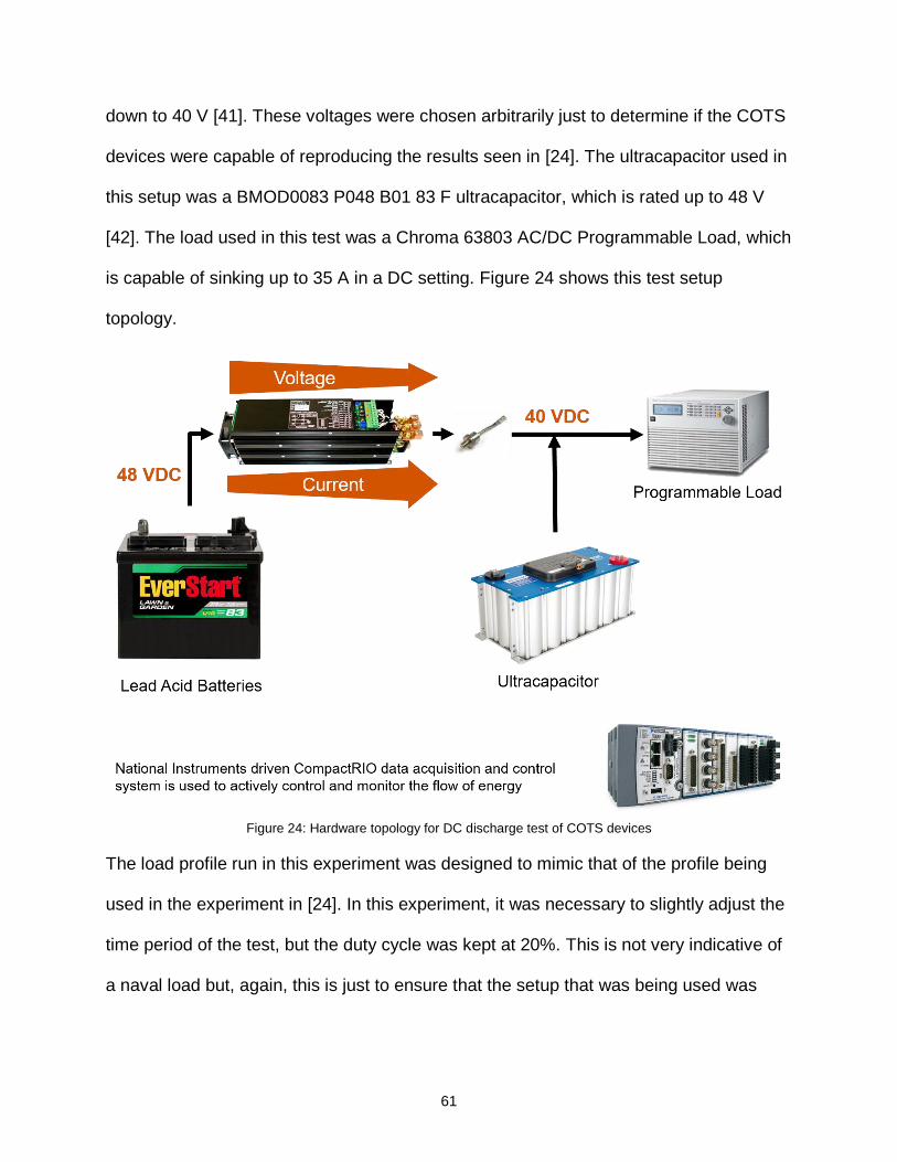
Using Figure 32 as a reference for the design, it is clear that the main changes on the
system come in the form of the loading and the power generation. For the load, there
was a shift to a Chroma 63803 AC programmable load with ratings of 3.6 kW / 36 A /
350 V, which is used to simulate the pulsed loads of interest. The AC load is controlled
dynamically using the GPIB protocol. In the results presented later, a 5 sec ‘on’ / 1 sec
‘off’ profile is run in which the AC programmable load varies its resistance from 9.6 Ω to
1 kΩ. To convert the DC power of the HESM into AC, a 4 kW Schneider Electric Conext
XW 4024 Inverter [43] is used. Its DC input voltage can vary from 20 – 32 VDC. One
74
feature heavily utilized is its ‘generator support’ feature that enables the system to draw
power from the generator up to a pre-specified current limit before starting to demand
power from the DC input. The generator is a 3000W Champion Power Equipment
gasoline generator. This generator outputs power in the form of a 120 VAC / 60 Hz
sinusoidal waveform. The frequency of the generator is dependent on the governor,
which compensates for loading effects to get the frequency as close as possible to 60
Hz. While the inverter technically has the ability to direct power flow from the generator
to the DC load bus, it takes a lengthy amount of time to switch between its charge and
discharge modes of operation. This is because the inverter was designed for residential
use and as such, changes in power flow tend to be made on the order of minutes rather
than milliseconds. In order to overcome this limitation, Xantrex XHR 33 VDC – 33 ADC
bench top power supplies are used to rectify the generator’s AC power and put it on to
the DC bus. The bench top DC power supplies are tied on to the DC load bus via an
IGBT switch. While the pulsed load is inactive, during the 1 sec ‘off’ time, the IGBT is
closed allowing the generator to remain base loaded as it puts power onto the DC load
bus. Once connected to the DC bus, the power supplies supply a recharge current back
to the batteries via the upper current path previously shown just to the right of the
batteries. Moving from the previous test to an AC setting required no changes on the
interactions between the batteries and the DC load bus, but the battery was swapped
out for a lithium-ion battery pack. The batteries being used are K2 LiFePO4 cells
arranged in a 12 series / 6 parallel configuration. They are 2.6 Ahr cells that have a
voltage range of 2.0 – 3.7 V [44]. By the transitive property, this means that the cells are
configured into 15.6 Ahr module with a voltage range of 24 – 43.8 V.
75
Figure 32: Hardware topology of the AC test of a COTS HESM [34]
At this point, it would be logical to think that the lithium-ion batteries might be suitable to
serve as a power dense module to either the lead-acid batteries or just to operate as a
standalone module, but in this scenario it is used as the energy dense device to keep
the current limited and the lifetime high. A Maxwell BMOD EDLC module is placed
across the DC load bus to serve as the power dense element capable of sourcing and
supplying any high power transients [42]. The module has an 83 F capacitance and a
voltage rating of up to 48 VDC. This was a module already owned by the lab and is not
optimized due to the vast spread between its maximum voltage ratings and that of the
DC bus. When used here, it typically remains within the range of 23 – 25 VDC.
76
This ultracapacitor has a maximum energy storage capability of
𝐸𝑛𝑒𝑟𝑔𝑦 =1
2𝐶𝑉2 =
1
2(83 𝐹)(48 𝑉)2 = 47.81 𝑘𝐽 ( 105 )
While Joules can be difficult to convert to Ahr on a capacitor due to its varying voltage
during operation, it could be assumed that the average voltage is the middle point of the
charged and discharged voltage, at 24 V.
𝐶𝑎𝑝𝑎𝑐𝑖𝑡𝑦 =
12𝐶𝑉𝑐ℎ𝑎𝑟𝑔𝑒𝑑
2
𝑉𝑎𝑣𝑒𝑟𝑎𝑔𝑒=
12
(83 𝐹)(48 𝑉)2
24 𝑉= 1.11 𝐴ℎ𝑟 ( 106 )
Although this is a considerable amount of capacity when compared to a traditional
capacitor, it is almost 15 times less energy than is stored in the lithium-ion battery pack.
On the other hand, while the K2 power cells have been experimentally shown to last up
to several hundred cycles during high rate cycling [19], the Maxwell Ultracapacitors are
rated up to 1,000,000 cycles at high rate cycling [42]. For these reasons, the HESM
uses the lithium-ion battery pack as the energy dense device and the ultracapacitor as
the power dense device. As before, since the EDLC is the only device on the load bus
without any current limitations placed on it, it dominates the voltage of the DC load bus.
If the EDLC loses charge, it follows that the DC load bus loses voltage. Therefore, the
purpose of the EDLC is to supply and absorb all transient currents without losing or
gaining a large amount of charge which might put the system outside of voltage
requirements dictated by the inverter.
Energy management is achieved using a National Instruments 9022 cRIO controller.
The cRIO has analog inputs, which are used to measure the power flow and voltage
points of the system in order to make a decision based on hierarchical importance. The
77
cRIOs are capable of altering the output voltages and current limits of the converters on
the fly as necessary. The priority hierarchy is as follows:
1. The control system’s highest priority is to maintain the charge voltage of the
batteries and EDLC. If the system detects that the battery voltage drops below a
preset value, it will shut down the HESM to protect the batteries. This is achieved by
sending a disable signal to all of the converters and all switches are open circuited. If
the EDLC module’s voltage drops below 20 VDC, the inverter will no longer accept
the DC load bus as a power input to the inverter. In an effort to get the HESM back
into operation, energy is fed from the batteries into the capacitor until its voltage is
restored.
2. The second highest priority of the control system is to deliver power to the load. Any
time power is demanded from the load, the HESM is automatically transitioned from
its current state into the discharge state so long as none of the safety conditions
listed in in Priority 1 above are violated.
3. The control system makes any attempt possible to recharge the batteries and/or
EDLC when power is available. This state of the system is only engaged when there
is a power supply available, there is no load demand, and none of the safety
conditions listed in in Priority 1 above are violated.
78
Figure 33: Experimental setup of the AC test of a COTS HESM [34]
The purpose of the experiments presented here is to demonstrate how a HESM may be
utilized in combination with a mechanical fossil fuel electrical generator to drive a high
power pulsed load. An load profile similar to the previous experiment was chosen and
can be seen in Table 7.
Table 7: Load Profile for HESM AC COTS Experiment
Period Time Value
First half of test
High Power 5 seconds 1500 W
Low Power 1 second 0 W
79
A few different scenarios will be explored in this report.
1. The first scenario utilizes the gasoline generator as the sole source in the
system. This scenario is hard on the generator as it is repetitively loaded and
unloaded.
2. In the second scenario, the generator is the sole power source, however instead
of being unloaded during the 1 second ‘off’ period, the HESM is employed as a
load to the generator keeping it base loaded as much as possible.
3. In the third scenario, the HESM and the generator simultaneously source power
to the load in a shared configuration and the HESM still sinks power from the
generator during the ‘off’ period in order to maintain the base loading of the
generator. This scenario ensures that the HESM is always able to accept charge
but if not properly configured, the HESM will source more capacity than it sinks
meaning that it will be depleted in the long run.
The intent is that these two latter scenarios will have a positive impact on the power
quality as opposed to that observed in the first scenario. Though not shown here,
additional scenarios are possible with a few being that the HESM is used alone to
source the load without a generator present or the HESM is used similar to the way it is
used in any of the scenarios listed but takes over the load only when a generator is
unavailable. The power quality delivered to the load, with regard to the frequency and
RMS voltage, will be presented.
80
Generator Only Test
The power flow of the system during the generator only experiment is seen in Figure 34.
In the plot, positive power implies that the source is supplying power while negative
power implies it is sinking power. The corresponding Fourier transform of the power
delivered to the load can be seen in Figure 35 and a plot of the RMS voltage delivered
to the load can be seen in Figure 36.
Figure 34: System power flow when only the generator is used to supply the load [34]
In Figure 34, it is clear that the HESM neither contributes nor accepts any power as the
generator handles the entire responsibility of powering the load. In Figure 35, it is shown
that two major frequencies are present during operation. Note that harmonics are also
measured, especially the third harmonic, however the focus will be placed on the shift in
fundamental frequency. The first dominant frequency is around 60.5 Hz and this is the
loading frequency. The unloaded frequency is around 62.5 Hz showing how the
81
transient nature of operation negatively affects the rotational speed of the generator.
The high frequency is observed less often simply because of the amount of time the
generator spends unloaded as opposed to the amount of time it spends loaded. For
comparison to standards, lines are drawn to show the constraints outlined in MIL-STD
1399 [45]. In Figure 36, the RMS voltage is shown along with the limits with which the
system must stay within in order to meet MIL-STD-1399. The system easily meets these
requirements with the only notable characteristics being the spikes of voltage when
there is a change in loading and the average voltage deviation during these periods.
During the ‘on’ period, the average voltage is around 120 V RMS while during the ‘off’
period, the average voltage is around 122.6 V RMS. This is a 2.6 V RMS difference
between these periods.
Figure 35: Fourier transform of power delivered to the load when only the generator is used to supply the load [34]
82
Figure 36: RMS load voltage when only the generator is used to supply the load [34]
Generator with Recharge Test
The power flow of the system during the second scenario experiment is seen in Figure
37. The corresponding Fourier transform of the power delivered to the load can be seen
in Figure 38 and the RMS voltage delivered to the load can be seen in Figure 39. Figure
37 shows how the generator sources the entire load during the ‘on’ period as well as the
HESM during the ‘off’ period. Note how there is a small amount of time between
transitions where the HESM switches states in reaction to the change in the load. Also
notice that despite the desire to base load the generator during the 1 second ‘off’
periods, this is not the case. This occurs for a couple of reasons. First, the current into
the batteries must be limited to 30 A corresponding to a 2C rating. This requires that the
buck converter output 1311 W, 43.7 V and 30 A.
83
Figure 37: System power flow when only the generator is used to supply the load and the HESM loads the generator during recharge [34]
The bench top power supplies are rated at 1 kW each making them ideally capable of
meeting the demand however their response is much slower than is needed to
accommodate the 1 second loading period. If they are fully loaded, the output current
quickly reaches 15 A, which is roughly half of their rated output current, however the
output slowly ramps up to the peak current over a duration of roughly a few seconds.
This means that the generator’s output is quickly reduced and then ramps up along with
them preventing its output from remaining as constant as desired. Before they reach the
demand required from them, the ‘off’ period has concluded and the HESM transitions
back into the sourcing state. In these tests, the power supplies were limited to 15 A so
that their output remained constant during the 1 second period therefore the generator
is also constant but less than that sourced by it to the load preventing it from being
84
equally loaded throughout the experiment. While the load power could have been
reduced to better demonstrate capability here, the experiment is presented as is to
show some of the tradeoffs that must be considered when designing such a system. In
the future, the power supplies will be replaced with a faster rectifier and the current will
be controlled using the recharge buck converter already in place. Another consequence
of the inability to base load the system is that the EDLC actually supplies the remaining
charge current to the batteries. This reduces their voltage prior to the next 5 second ‘on’
period which is undesirable. One proposed fix is to actively control the capacitor using
additional power electronics and this is also planned in future work.
Comparing Figure 38 to Figure 35, it is clear that the frequencies start to shift closer to
60.5 Hz however there are still times where the frequency is closer to 62.5 Hz. This shift
closer to 60.5 Hz is due to the HESM’s ability to more evenly balance the base loading
of the generator. As improvements are made to the system, it is expected that the
generator can be better base loaded and all frequencies away from the load frequency
can be reduced if not nearly eliminated. At first glance, it appears that the RMS voltages
in Figure 39 are identical to those in Figure 35. However, upon closer inspection it
becomes obvious that while there are still transient spikes during the transition phases,
the average voltages converge slightly. During the ‘on’ period, the average voltage is
around 121.5 V RMS while during the ‘off’ period, the average voltage is around 122.3 V
RMS. This is only a 0.8 V RMS difference, as opposed to the 2.6 V RMS difference
measured during the generator only experiment. As it did earlier, the RMS voltage
always stays within the constraints of MIL-STD-1399.
85
Figure 38: Fourier transform of power delivered to the load when only the generator is used to supply the load and the HESM loads the generator during recharge [34]
Figure 39: RMS load voltage when only the generator is used to supply the load and the HESM loads the generator during recharge [34]
86
Generator and HESM Parallel Test
The final experiment presented here is one in which the generator and the HESM are
simultaneously used to source power to the load and the HESM is used to absorb
energy from the generator during the load’s 1 second periods of inactivity. The flow of
power from each source during the experiment is plotted in Figure 40. The
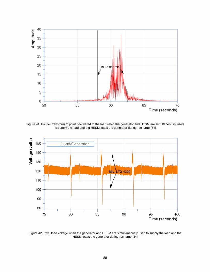
corresponding Fourier transform of the power delivered to the load is seen in Figure 41
and the RMS voltage delivered to the load is seen in Figure 42.
Figure 40: System power flow when the generator and HESM are simultaneously used to supply the load and the HESM loads the generator during recharge [34]
In parallel operation, the Xantrex inverter’s ‘generator support’ function is used to limit
the power flow from the generator and simultaneously source power from the inverter’s
DC input source. This is achieved by setting a limit on the RMS current that the inverter
draws from the generator. If the RMS current limit is exceeded, the inverter kicks in and
augments the generator with power from the DC source. Whenever the inverter’s load
87
transitions from an ‘off’ state to an ‘on’ state, the inverter immediately sources all of the
load’s demand by passing through power from the generator. Unfortunately, as it does
this the inverter does not quickly limit power from the generator meaning that if the load
immediately demands power in excess of the ‘generator support’ limit, the generator will
be stressed beyond the desired limits. Once the inverter detects that the ‘generator
support’ limit has been exceeded, it takes the inverter just over two seconds before it
fully limits the generator and augments it with power from the battery. While this is
acceptable in most steady state applications, it is not optimal when pulsed loads are
being operated. In the experiments presented here, roughly half of the pulsed load ‘on’
time has passed before the generator is limited and the batteries start to source power
to the load. This type of operation is seen in Figure 40 where the generator’s output
power quickly spikes up and then ramps down in just over two seconds while the HESM
slowly ramps up. Eventually both sources supply equal amounts of power, however it is
much later than is needed to maintain a stable base load on the generator. The
opposite is also true in that once the load turns off and DC power is no longer needed, it
takes the inverter some time to recognize this and stop drawing power from the DC
input. These are all consequences of using COTS components within the HESM design
rather than those which are custom designed.
Figure 41 shows that the frequencies are closer to 60 Hz, similar to the ‘Generator with
Recharge’ test. The spikes previously seen around 60.5 Hz and 62.5 Hz are still present
but there is a clear shift towards 60 Hz. These results aren’t completely representative
of what this setup is capable of providing if the inverter response is faster, but they are
still better than the results from the ‘Generator Only’ test.
88
Figure 41: Fourier transform of power delivered to the load when the generator and HESM are simultaneously used to supply the load and the HESM loads the generator during recharge [34]
Figure 42: RMS load voltage when the generator and HESM are simultaneously used to supply the load and the HESM loads the generator during recharge [34]
89
As seen in Figure 42, there is a glaring difference in the RMS voltage waveform with
presence of enormous voltage spikes and sags during transition when the load
transitions from an ‘on’ state to an ‘off’ state. The sags are due to the overloading of the
generator while it must source both the load and the HESM. The spikes are due to the
abrupt open circuit after removing both of these loads. It is important to note that these
voltage spikes and sags bring the system outside of the standards set by MIL-STD-
1399.
The work presented here provides a brief glimpse into the design of a HESM and shows
a few of the operational scenarios in which it will be utilized in the Navy’s future electric
fleet. The experiments showed how the operation of pulsed loads using a mechanical
generator alone imparts high stress on the generator and results in poor power quality.
They have also shown how a generator can be better base loaded if a HESM is used as
the generator’s load during periods of load inactivity. Similarly, it has been shown how a
HESM can be used to augment a generator to supply the load while maintaining a base
load on the generator. The latter set of results presented did not fully achieve the
desired results and give a false impression that a HESM actually negatively impacts
power quality. This is purely a result of two drawbacks introduced to the UTA system
through the use of COTS components. This problem can be overcome by simply
avoiding COTS software for integrating AC power sources and by rectifying the power
from the generator to join the two power sources together in a DC setting before
inverting them back to AC for transferring to another part of the ship. Now that the
topology of the HESM using COTS equipment has been verified, the final logical step in
this work is to analyze the ability of the fuzzy logic controller to impose a system level
90
control over the COTS equipment, solidifying the proposed hypothesis that it is a viable
solution to this application.
Fuzzy Logic Control of COTS Equipment Test
The final experiment presented here is one in which the entire work presented here has
built up to. It is easy to say that a system or a controller will work by designing and
simulating the results, but it may prove to be much more difficult to implement when
using real world products with their own internal control systems and dynamics to
account for. In a final effort to validate the candidacy of a fuzzy logic control for
implementing system level control over a Hybrid Energy Storage Module, it was decided
to utilize the controller on the COTS HESM.
The system was completely physically overhauled in order to clean up the wiring, place
the newer National Instruments 9118 CompactRIO Controller, and remove unnecessary
components such as pull-boxes and extra Anderson Connectors. Photos of the new
setup can be seen in Figure 43, Figure 44, and Figure 45. Figure 43 shows the overall
COTS HESM System. Starting from the left and moving to the right, the HESM utilizes a
PC with a fiber optic connection through the PCI-E slot to a National Instruments PXI-e
1078 chassis with NI PXI-e 6361 analog input modules for data acquisition. These
modules are capable of up to 2 GHz sample rates, but in these tests they will only be
used to sample at rates of about 1 KHz. The connections to these modules are attached
to the side of the PC cart as BNC connectors. To the right and front of the PC is the
energy storage cart. On the left of the cart are the battery packs in a blue shrink wrap.
This is the same K2 lithium-ion 12s/6p battery pack used in previous tests.
91
Figure 43: Photo of Overall COTS HESM System
The next device is the 500 F 16 V Ultracapacitor. This is not used in this test. The final
device is an 83 F 48 V Ultracapacitor which is the capacitor that sits on the 24 V DC
Load Bus in this test. Behind the energy storage cart is the actual HESM and can be
better seen in a close-up photo in Figure 44. On the top left of the photo, the National
Instruments 9118 CompactRIO Controller can be seen connected largely to the terminal
blocks below it. This can be seen much better in the close-up photo in Figure 45. To the
right of the controller, 5 separate black boxes can be seen which contain the switches
for the DC/DC power converters. These boxes connect to the green PCBs seen below
which are the LC filters for their respective power converters. Between the copper bus
bars, several yellow differential probes can be seen which are responsible for dividing
down the voltage of the busses for the data acquisition system.
92
Figure 44: Close-up photo of the HESM
At the bottom of the photo, several components can be seen. There are blue Anderson
Connectors which are used for connecting the energy storage devices, the inverter, and
the power supply to the HESM cart. Additionally, there are blue Automation Direct hall-
effect current sensors which return voltages between +/- 10 V proportional to the
amount of DC current flowing through the wires. Finally, there are grey DC contact
relays responsible for providing not only a controllable way to insert items to their
respective busses, but also as a quick emergency shutdown of the HESM cart. Looking
back at Figure 43 and moving to the right of the HESM, there is a Sorensen DCS40-75E
power supply capable of providing up to 40 V and 75 A of DC power. This is used to
93
mimic a generation source in the tests. Below the power supply is a Chroma 63803 AC
programmable load that receives power that is inverted through the Schneider Electric
Conext XW 4024 Inverter that is barely visible behind the HESM cart.
Figure 45: Close-up of the NI Controller
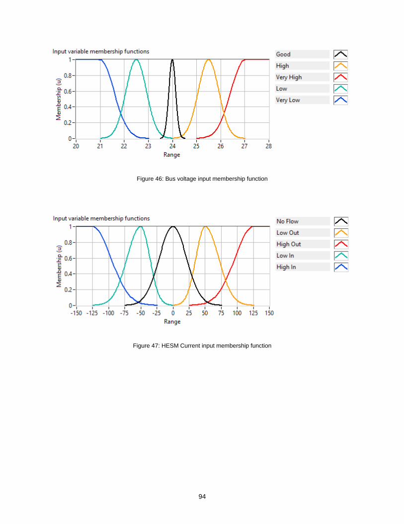
Another change in the experimental setup was the fuzzy logic controller. In this system,
it was necessary to use a 24 V DC load bus and a ~40 V battery bus with a much higher
current capacity so the controller was redesigned and can be seen in further detail in
Figure 46, Figure 47, and Figure 48. More detail about the specifics of each
membership function can be seen in Table 8.
94
Figure 46: Bus voltage input membership function
Figure 47: HESM Current input membership function
95
Figure 48: Battery Current output membership function
Table 8: Numerical descriptions of membership functions
Input/Output Linguistic Value Range
Input 1 “Very Low” < ~23 V
Input 1 “Low” 21 V – 24 V
Input 1 “Good” 23.5 V – 24.5 V
Input 1 “High” ~24 V – ~27 V
Input 1 “Very High” > 25 V
Input 2 “High In” < -25 A
Input 2 “Low In” -125 A – 0 A
Input 2 “No Flow” -75 A – 75 A
Input 2 “Low Out” 0 A – 125 A
Input 2 “High Out” > 25 A
Output “High Recharge” < -50 A
Output “Low Recharge” ~-100 A – 0 A
Output “No Flow” -25 A – 25 A
Output “Low Discharge” 0 A – 100 A
Output “High Discharge” > 50 A
96
To test this system, a similar profile was designed to replicate the results of the tabletop
experiments. In this case, the easiest way to use the programmable loads was to
command them to operate in a constant resistance setting for a specified amount of
time. The load profile run can be seen in Table 9.
Table 9: Load profile for the COTS HESM fuzzy logic control experiment
Period Time Value
First half of test
High Power 5 seconds 5 Ω
Low Power 1 second 1000 Ω
Second half of test
High Power 5 seconds 25 Ω
Low Power 1 second 1000 Ω
The results of the experiment can be seen in Figure 49 and Figure 50. These results
show that the fuzzy logic controller is excellent at maintaining the bus voltage as shown
in the tabletop tests. The current plots follow very similar results to the tabletop
experiments and this can be considered an overall successful implementation of the
controller.
97
Figure 49: Voltage plot from COTS HESM fuzzy logic control test
Figure 50: Current plot from COTS HESM fuzzy logic control test
98
Chapter 6: Summary and Conclusions
ESDs are becoming more and more crucial as integrated power systems evolve. Their
application in naval settings are becoming more desirable and the challenges
associated with individual ESDs can be overcome by utilizing a HESM topology. The
work presented here aimed to not only demonstrate the design of a Hybrid Energy
Storage Module, but to present a method of control for such a system, even while using
commercial-off-the-shelf components as might be seen in a real world application. This
work has shown that fuzzy logic control was capable of controlling this system through
each level of construction from a model, to a custom tabletop testbed, and finally to a
COTS system integration. While all of this has been demonstrated in a laboratory setup,
much of the design can be largely transferred to practical application designs in future
systems with very minor additional considerations. It is not expected that COTS
components will ever flawlessly achieve all of the unique demands of this type of
system, but the work shown here has identified some of the shortcomings of COTS
technologies while simultaneously showing many of the exciting benefits that a HESM
offers to future naval power application. This work will be used to ensure that a future
custom solution is able to meet all of any unique demands required of a shipboard naval
HESM.
100
Operation Manual for Controlling Xantrex XHR 33-33 for HESM Tabletop
Tests
1. Ensure that the GPIB to USB cable is connected to both the power supply and
the controlling computer
2. Ensure that the power supply is powered on
3. Open LabVIEW project file from Tabletop HESM > LabVIEW >
PowerSupplyControl-TabletopHESM.lvproj
4. Open PowerSupplyControl-TabletopHESM.vi
You will be presented with a VI that looks like Figure 51.
Figure 51: VI of Xantrex XHR 33-33 GPIB Control
5. Click the dropdown button and select the Xantrex XHR 33-33 GPIB resource.
101
This resource name may not be obvious. If you are confused and there are several
devices available to choose from, try to use NI MAX to get a better idea of which
resource is the power supply.
6. Type in a value for the voltage setpoint
7. Type in a value for the current limit high
8. Type in a value for the current limit low
9. Type in a value for the high time
10. Type in a value for the low time
11. Press play on the VI controls
12. When ready, press the enable power supply button
13. When test is complete, press the stop button
The descriptions of the buttons and indicators, starting from the top left and moving to
the bottom right, are as follows:
Stop button – Stops the VI when it is being run. This will also shut
down the visa connection.
Error # - This indicator shows the user what error code number is
being returned by the power supply (if one is present). Error codes can
be referenced in the XHR 33-33 user manual.
VISA Resource Name – Selects the GPIB connections to the power
supply.
Voltage Setpoint – this allows the user to select what level of voltage
they would like the power supply to attempt to achieve (keep in mind
102
that this voltage will be automatically rolled back by the power supply if
the current limits set in the next fields are exceeded).
Current Limit High – This allows the user to select how much current
the power supply should be limited to during “high” times.
Current Limit Low – This allows the user to select how much current
the power supply should be limited to during “low” times.
Enable Power Supply – This button allows the user to enable the
output of the power supply. If this button is not pressed, the power
supply will remain in standby mode.
High Time – This allows the user to select how much time, in seconds,
they would like the power supply to remain in “high” time (the total time
of a repeated period is the summation of “high” time and “low” time).
Low Time - This allows the user to select how much time, in seconds,
they would like the power supply to remain in “low” time (the total time
of a repeated period is the summation of “high” time and “low” time).
STATE – This indicates to the user the current state of the program
and flips between “High” and “Low” depending on the state.
103
Operation Manual for HESM Tabletop Software
1. Ensure that the PC104 is powered on and the Ethernet cable is connected to the
controlling computer
2. Open the Simulink file in Tabletop HESM > MATLAB > xPC >
xPC_HESMwithFuzzy_LPF.slx
You will be presented with a “model” that looks like Figure 52.
Figure 52: Simulink software for running the HESM tabletop
3. Press the “Build Model” button . This will compile the Simulink code into C
code and deploy it onto the PC104.
4. Press the “Connect to Target” button .
5. Press the “Play” button .
6. Use the power supply as described in the Operation Manual for Controlling
Xantrex XHR 33-33 for HESM Tabletop Tests section in Appendix A.
104
The PC104 being used in this tabletop testbed is seen in Figure 53. The top module is
the PC104 PC running Simulink RTOS. It contains an Intel Atom N455 1.66 Ghz Single
Core Processor and has 1 GB DDR3 800 MHz onboard memory. The second module
moving down is the MPL PATI-1 PWM board. This board has 32 PWM channels that
can operate independently of each other. The third module down is the Diamond DMM-
32X-AT Analog Input board. This board has channels for Analog I/O and Digital I/O, but
in this setup, only the Analog Inputs are being used. On the Analog Inputs, channel 1
and 2 are broken so everything is shifted over starting at channel 3.
Figure 53: PC104 target PC for HESM tabletop experiments
105
The color scheme of the software is as follows:
Grey blocks – These are blocks directly associated with the PC104
target PC. These are either settings blocks or direct I/O interfacing
blocks.
Green blocks – These blocks are associated with signal input and
conditioning. These blocks are responsible for filtering the signals,
applying their gains, and setting the variables to be used by other
blocks.
Orange blocks – These blocks are associated with reading variables.
They are used as control inputs and for indicators on the GUI for the
user to validate what they think they should be seeing. The indicators
do not update very quickly, so the important values are actually sent to
the PC104 for a virtual scope that is displayed on a VGA connected
monitor.
Purple blocks – These blocks are associated with controls. These
controls are not interactive with the user and are essential in voltage
control, current limiting, and fuzzy logic control of the tabletop.
Blue blocks – These blocks are associated with user interactive
controls. The constant blocks are used to set how many clock cycles
on a 10 MHz clock will be used for ‘on’ and ‘off’ times of the switch.
The percentage of ‘on’ time over ‘off’ time is the duty cycle of the
switching converter. These are only used if the Manual switch is in the
106
up position. If the manual switch is in the lower position, it will defer to
the purple control blocks.
The descriptions of the most important buttons and indicators, starting from the top left
and moving to the bottom right, are as follows:
MM-32 Diamond Analog Input – Direct access to the analog I/O pins
on the PC104. These analog values can range from -10 to 10 V and
they start at a base address of 0x300. This is configured as differential
inputs for pins 1-16 and the first channel used in this software is
channel 3.
Filters – These blocks are used as low-pass filters for all the signals
coming from the HESM tabletop. The time constant for the filter is set
at 10 ms.
PATI MPL Timebase Setup – This sets the frequency for the PWM
generator on the PATI board. For this software, only the TCR1 timer is
used, so the PATI board clock is set to 10 MHz so each period is 100
ns.
PATI MPL PWM Generate – This block is responsible for generating
the PWM signal for the switches. The H input on the blocks correspond
to the periods of the 10 MHz clock that the PWM signal will remain
high and the L input corresponds to the periods of the 10 MHz clock
that the PWM signal will remain low. High always comes before low.
They should add up to the desired period of the switching frequency.
107
Control blocks – These blocks are set up with two separate loops of
control. One loop is for buck converter control (top) and one is for
boost converter control (low). Only one loop can be active at a time,
which is dictated by the sign of the fuzzy logic controller output and
controlled with the software switches. Both of these controllers output
to a variable that is accessed by the PWM generator blocks, but also to
a target scope, which is responsible for outputting the waveform to a
VGA connected monitor on the PC104.
Measurement blocks – These blocks not only give a front panel read
out of the voltages and currents that update slowly, but also output all
voltages and currents to target scopes which, like above, output the
waveform to a VGA connected monitor on the PC104.
108
Operation Manual for COTS HESM Software
1. Turn on the PXI chassis
2. Turn on the control and data acquisition PC
3. Go to “E:\Dropbox\UTA PPEL Team Folder\Projects\COTS
HESM\LabVIEW\Newest HESM”
4. Open “HESM.lvproj”
5. Open “PXI-QuickStart.vi”, click run, and minimize the VI (seen in Figure 54)
Figure 54: PXI-QuickStart.vi Front Panel
6. Open “RunLoadProfile.vi”, select the file for the programmable load, and click run
(seen in Figure 55)
To edit the file:
a. Go to the file location (“E:\Dropbox\UTA PPEL Team
Folder\Projects\COTS HESM\LabVIEW\Chroma AC Control”)
b. Open the file using excel for ease, but the file can be edited in notepad
c. Follow convention to make edits
109
To change the file during operation
a. Select file from file browser
b. Click reload data file
Figure 55: RunLoadProfile.vi Front Panel
7. Press the “plus” button to the left of the cRIO target “newHESM”
8. Open “Main.vi” and click run (seen in Figure 56)
110
Figure 56: Main.vi Front Panel
9. Use the relay control box to insert the power sources desired
10. Set the current limiters if manual operation is desired
11. Enable the desired converters if manual operation is desired
12. Fill in the file name box, the sample rate, and the run time of the test in the Data
Acquisition box if data recording is desired
13. Select the control type if Fuzzy Logic Control is desired
a. Note: This mode does not utilize the active capacitor
14. Press record to initiate the test
a. Note: This button turns on and off the recording of the PXI chassis and it
initiates the programmable load profile all by network variables – it
requires no human intervention.
111
15. If anything causes great concern, the emergency stop button can be used to
open all relays and disable all converters without stopping the program, use this
only in emergencies as it can degrade the lifetime of the relays
16. When finished using, the stop vi button in the top right will also ensure that all
converters are disabled and that all relays are open before shutting down the VI
112
References
[1] D. Stoudt, "Naval Directed-Energy Weapons - No Longer a Future Weapon
Concept," Leading Edge, vol. 7, no. 4, pp. 6-11, 2012.
[2] H. Fair, "Progress in Electromagnetic Launch Science and Technology," IEEE
Transactions on Magnetics, vol. 43, no. 1, pp. 93-98, 2007.
[3] H. Fair, "Advances in Electromagnetic Launch Science and Technology and its
Applications," IEEE Transactions on Magnetics, vol. 45, no. 1, pp. 225-230, 2009.
[4] J. Kuseian, "Naval Power Systems Technology Development Roadmap PMS 320,"
May 2013. [Online]. Available:
http://www.navsea.navy.mil/Media/Forms/AllItems.aspx. [Accessed 2014].
[5] N. Doerry, "Next Generation Integrated Power System NGIPS Technology
Development Roadmap," November 2007. [Online]. Available:
http://www.dtic.mil/cgi-bin/GetTRDoc?AD=ADA519753. [Accessed 2014].
[6] W. Matthews, "Navy: Energy Weapons Ready for Ships," May 2013. [Online].
Available: http://seapowermagaizine.org/sas/stories/20130410-energy-
weapons.html. [Accessed 2014].
113
[7] J. Thongam, "All-electric ships - A review of the present state of the art," in 8th
International Conference and Exhibition on Ecological Vehicles and Renewable
Energies, 2013.
[8] Y. Chuan, G. Venayagamoorthy and K. Corzine, "AIS-Based Coordinated and
Adaptive Control of Generator Excitation Systems for an Electric Ship," IEEE
Transactions on Industrial Electronics, vol. 59, no. 8, pp. 3102-3112, 2012.
[9] J. Gully, "Investigation of an Alternator Charged Pulse Forming Network with
Flywheel Energy Storage," IEEE Transactions on Magnetics, vol. 29, no. 1, pp.
969-974, 1993.
[10] D. Swett and J. Blanche, "Flywheel charging module for energy storage used in
high-voltage pulsed and multi-mode mobility hybrid electric military vehicle power
system," in Conference Record of the 2004 Power Modulator Symposium and
2004 High Voltage Workshop, 2004.
[11] J. Ennis, "Recent Advances in High Voltage, High Energy Capacitor Technology,"
in 16th IEEE International Pulsed Power Conference, San Diego, 2007.
[12] H. Boenig, "Design and testing of high power reptitively pulsed, solid-state closing
switches," in Industry Applications Conference, Thirty-Second IAS Annual Meeting,
IAS '97, 1997.
114
[13] S. Balathandayuthapani, C. Edrington and S. Henry, "Study on converter
topologies for capacitive pulse forming network and energy storage units in electric
ship," in 2011 IEEE Electric Ship Technologies Symposium (ESTS), 2011.
[14] R. Kotz and M. Carlen, "Principles and Applications of Electrochemical
Capacitors," Electrochimica Acta, vol. 45, pp. 459-462, 2000.
[15] P. Novak, D. Wetz and B. Shrestha, "Cycling Fatigue induced on Electrochemical
Energy Storage Cells as a result of High C Pulsed Charging," Electrochemical
Society Transactions, vol. 50, no. 26, pp. 175-186, 2013.
[16] D. Wetz, B. Shrestha and P. Novak, "Pulsed Evaluation of High Power
Electrochemical Energy Storage Devices," IEEE Transactions on Dielectrics and
Electrical Insulation, vol. 20, no. 4, pp. 1040-1048, 2013.
[17] Saft America, Inc., "Rechargeable lithium-ion battery VL 5U - Ultra high power cell;
Doc. No. 54073-2-1009," 2009.
[18] B. Shrestha, D. Wetz and P. Novak, "The Impact of High Pulsed Loading on the
Fatigue of Electrochemical Energy Storage Devices," Electrochemical Society
Transactions, vol. 50, no. 26, pp. 187-196, 2013.
[19] D. A. Wetz, B. Shrestha, S. T. Donahue, D. N. Wong, M. J. Martin and J. M.
Heinzel, "Capacity Fade of 26650 Lithium-Ion Phosphate Batteries Considered for
Use Within a Pulsed-Power System's Prime Power Supply," Plasma Science,
IEEE Transactions on, vol. 43, pp. 1448-1455, 2015.
115
[20] M. Hantel, Graphite Oxie and Graphene Oxide Based Electrode Materials for
Electrochemical Double Layer Capacitors, Munich: Technische Universität
München, 2013.
[21] D. Shin, "Battery-Supercapacitor Hybrid System for High-Rate Pulsed Load
Applications," in Design, Automation & Test in Europe Conference & Exhibition,
2011, 2011.
[22] L. Baoquan, Z. Fang and B. Xianwen, "Control Method of the Transient
Compensation Process of a Hybrid Energy Storage System Based on Battery and
Ultracapacitor in Micro-grid," in IEEE International Symposium on Industrial
Electronics, 2012.
[23] A. Khaligh and Z. Li, "Battery, Ultracapacitor, Fuel Cell, and Hybrid Energy Storage
Systems for Electric, Hybrid Electric, Fuel Cell, and Plug-In Hybrid Electric
Vehicles: State of the Art," IEEE Transactions on Vehicular Technology, vol. 59,
no. 6, pp. 2806-2814, 2010.
[24] L. Gao, R. A. Dougal and S. Liu, "Power Enhancement of an Actively Controlled
Battery/Ultracapacitor Hybrid," Power Electronics, IEEE Transactions on, vol. 20,
no. 1, pp. 236-243, 2005.
[25] I. J. Cohen, J. P. Kelley, D. A. Wetz and J. Heinzel, "Evaluation of a Hybrid Energy
Storage Module for Pulsed Power Applications," Plasma Science, IEEE
Transactions on, vol. 42, no. 10, pp. 2948-2955, 2014.
116
[26] S. M. Lukic, S. G. Wirasingha, F. Rodriguez and J. Cao, "Power Management of
an Ultracapacitor/Battery Hybrid Energy Storage System in an HEV," in IEEE
Vehicle Power and Propulsion Conference, 2006. VPPC '06, Windsor, 2006.
[27] D. Carreira, G. D. Marques and D. M. Sousa, "Hybrid Energy Storage System with
a Low Cost Digital Control," in 2015 9th International Conference on Compatibility
and Power Electronics (CPE), Costa da Caparica, 2015.
[28] C. Jin, N. Lu, S. Lu, Y. Makarov and R. Dougal, "Coordinated Control Algorithm for
Hybrid Energy Storage Systems," in 2011 IEEE Power and Energy Society
General Meeting, 2011.
[29] V. B. Semwal, P. Chakraborty and G. C. Nandi, "Less computationally intensive
fuzzy logic (type-1)-based controller for humanoid push recovery," Robotics and
Autonomous Systems, vol. 63, no. 1, pp. 122-135, 2015.
[30] Y. Lu, H. L. Hess and D. B. Edwards, "Adaptive Control of an Ultracapacitor
Energy Storage System for Hybrid Electric Vehicles," in IEMDC '07, IEEE
International Antalya: Electric Machines and Drives Conference, 2007.
[31] C. H. Wu, P. Y. Chen and J. C. Ke, "On the Study of Energy-Based Control
Strategy for a Lithium Battery/Supercapacitor Hybrid Energy Storage System," in
2010 International Conference on Environmental Science and Information
Application Technology (ESIAT), Wuhan, 2010.
117
[32] Z. Yu, Z. Jiang and X. Yu, "Control Strategies for Battery/Supercapacitor Hybrid
Energy Storage Systems," in IEEE Energy 2030 Conference, Atlanta, 2008.
[33] D. G. Wilson, R. D. Robinett III and S. Y. Goldsmith, "Renewable Energy Microgrid
Control with Energy Storage Integration," in 2012 International Symposium on
Power Electronics, Electrical Drivers, Automation and Motion (SPEEDAM),
Sorrento, 2012.
[34] I. J. Cohen, D. A. Wetz, C. Storm and J. Heinzel, "Impact of a Hybrid Energy
Storage Module on Power Quality of a Fossil Fuel Generator," in Proceedings of
the 2014 American Society of Naval Engineers Electric Machines Technology
Symposium (EMTS), Philadelphia, 2014.
[35] Y. Zhang, J. Zhenhua and Y. Xunwei, "Small-Signal Modeling and Analysis of
Battery-Supercapacitor Hybrid Energy Storage Systems," in IEEE Power & Energy
Society General Meeting PES '09, Calgary, 2009.
[36] V. H. Johnson, A. A. Pesaran and T. Sack, "Temperature-Dependent Battery
Models for High-Power Lithium-Ion Batteries," in 17th Annual Electric Vehicle
Symposium, Montreal, 2000.
[37] T. J. Ross, Fuzzy Logic with Engineering Applications, McGraw-Hill, 1995.
[38] M. Sugeno, "An Introductory Survey of Fuzzy Control," Information Sciences, vol.
36, no. 1, pp. 59-83, 1985.
118
[39] C. C. Lee, "Fuzzy Logic in Control Systems: Fuzzy Logic Controller. II.," IEEE
Transactions on Systems, Man and Cybernetics, vol. 20, no. 2, pp. 419-435, 1990.
[40] NXP, "Designing RC snubbers - AN 11160," 2012.
[41] Zahn Electronics, Inc., "DC/DC Converters," 2015. [Online]. Available:
http://www.zahninc.com/dcdcsdsu1.html. [Accessed 22 September 2015].
[42] Maxwell Technologies, "48V Modules Datasheet," 2013. [Online]. Available:
http://www.maxwell.com/images/documents/hq_48v_ds10162013.pdf. [Accessed
22 September 2015].
[43] "Conext XW Inverters/Chargers," Schneider Electric, [Online]. Available:
http://www.schneider-electric.com/.
[44] K2 Energy, "High Capacity LFP26650P Power Cell Data," [Online]. Available:
http://liionbms.com/pdf/k2/LFP26650P.pdf. [Accessed 22 September 2015].
[45] MIL-STD-1399, Department of Defense, 2008.
[46] L. Gao, R. Dougal and S. Liu, "Active Power Sharing in Hybrid Battery/Capacitor
Power Sources," in Eighteenth Annual IEEE Applied Power Electronics
Conference and Exposition, 2003 (APEC '03), 2003.
119
Biographical Information
Isaac J. Cohen was born in Miami, Florida in 1988. He received the B.S. degree in
electrical engineering in 2013 from the University of Texas at Arlington and has spent
several summers serving as a research fellow at the Naval Surface Warfare Center in
Philadelphia, Pennsylvania. He served as Chair of the Student Branch of IEEE at UTA
in 2012, where he received several awards for his outstanding service. He currently
serves as Chair of the Young Professionals affinity group within the IEEE Fort Worth
Section. His research interests include applying control theory to power electronics in
microgrid, energy storage, and pulsed power settings.