+ All Categories
Home > Documents > THE DESIGN AND FABRICATION OF AN OMNI-DIRECTIONAL … · CHRISTOPHER ROBERT FULMER ... Craig and...

THE DESIGN AND FABRICATION OF AN OMNI-DIRECTIONAL … · CHRISTOPHER ROBERT FULMER ... Craig and...

Date post: 28-May-2019
Category:
Upload: dinhtruc
View: 219 times
Download: 0 times
Share this document with a friend
113
THE DESIGN AND FABRICATION OF AN OMNI-DIRECTIONAL VEHICLE PLATFORM By CHRISTOPHER ROBERT FULMER A THESIS PRESENTED TO THE GRADUATE SCHOOL OF THE UNIVERSITY OF FLORIDA IN PARTIAL FULFILLMENT OF THE REQUIREMENTS FOR THE DEGREE OF MASTER OF SCIENCE UNIVERSITY OF FLORIDA 2003
Transcript

THE DESIGN AND FABRICATION OF AN OMNI-DIRECTIONAL VEHICLE PLATFORM

By

CHRISTOPHER ROBERT FULMER

A THESIS PRESENTED TO THE GRADUATE SCHOOL OF THE UNIVERSITY OF FLORIDA IN PARTIAL FULFILLMENT

OF THE REQUIREMENTS FOR THE DEGREE OF MASTER OF SCIENCE

UNIVERSITY OF FLORIDA

2003

Copyright 2003

by

Christopher Robert Fulmer

ACKNOWLEDGMENTS

The author would like to thank all of those who made his years at the University of

Florida a memorable and interesting experience. In particular the author would like to

express his deepest gratitude to Dr. Carl Crane for the dedication he has for his students

and the engineering program as a whole.

The author would also like to thank Dr. John Zigert and Shannon Ridgway for their

guidance and many suggestions throughout the development of this project. Thanks go to

all the people of the Center for Intelligent Machines and Robotics for their help and

friendship.

The author would like to thank his parents, Craig and Patty Fulmer, for their

support and encouragement throughout the years. To his fiancee, Cindy, he wishes to

extend his most heartfelt love and gratitude for inspiring him to make the most out of this

opportunity.

iii

TABLE OF CONTENTS

page

ACKNOWLEDGMENTS ................................................................................................. iii

LIST OF TABLES............................................................................................................. vi

LIST OF FIGURES .......................................................................................................... vii

ABSTRACT....................................................................................................................... xi

CHAPTER

1 INTRODUCTION ........................................................................................................1

Omni-directional Vehicle Platforms............................................................................ 3 Special Wheel Designs ......................................................................................... 4 Conventional Wheel Designs ............................................................................... 6

Vehicle Criteria............................................................................................................ 7 Approach...................................................................................................................... 8 Background.................................................................................................................. 8

Permanent-Magnet Motors................................................................................... 8 Performance characteristics..........................................................................11 Cooling .........................................................................................................13 Position sensing............................................................................................14

Gearing ............................................................................................................... 15 Epicyclic gearing..........................................................................................15 Spur gears .....................................................................................................16

2 MOTOR AND GEAR TRAIN DESIGN ...................................................................21

Load ........................................................................................................................... 21 Motor Selection ......................................................................................................... 21 Controller Selection ................................................................................................... 24 Gear Train Design...................................................................................................... 25

Gear Backlash..................................................................................................... 27 Bearing Life........................................................................................................ 28 Motor Cooling .................................................................................................... 28 Gearing Features................................................................................................. 29

iv

3 DRIVE WHEEL HOUSING AND JOINT DESIGN.................................................32

Load Considerations .................................................................................................. 32 Joints .......................................................................................................................... 35

4 PERFORMANCE TESTING .....................................................................................39

Dynamometer ............................................................................................................ 39 Cooling ...................................................................................................................... 42 Data Acquisition ........................................................................................................ 43

5 RESULTS...................................................................................................................46

Speed/Torque Curves and Load Testing.................................................................... 46 Maximum Continuous Torque Testing...................................................................... 47 Acceleration............................................................................................................... 51 Energy Balance.......................................................................................................... 54 Thermal Resistance and Capacitance ........................................................................ 56 Motor Parameters and Constants ............................................................................... 58

6 SUMMARY AND CONCLUSIONS.........................................................................59

APPENDIX

A DIMENSIONAL DRAWINGS..................................................................................61

B GEAR DATA .............................................................................................................96

LIST OF REFERENCES.................................................................................................100

BIOGRAPHICAL SKETCH ...........................................................................................102

v

LIST OF TABLES

Table page 1-1 Epicyclic gear arrangements ...............................................................................16

1-2 Formulas for the dimensioning of spur gears .....................................................18

2-1 Thrust needed to translate a 400lb vehicle..........................................................21

2-2 Estimates for the physical properties of the wheel .............................................22

2-3 Manufacturing data for the 1st stage planetary arrangement...............................26

2-4 Manufacturing data for the 2nd stage planetary arrangement ...........................27

3-1 Maximum forces attainable for the wheel main bearings...................................35

5-1 Steady state averages for continuous torque test. ...............................................50

5-2 Drive wheel parameters ......................................................................................58

A-1 Bill of materials...................................................................................................94

B-1 Manufacturing data for 1st stage planetary arrangement.....................................96

B-2 Manufacturing data for 2nd stage planetary arrangement....................................97

B-3 Backlash considerations for 1st stage of the epicyclic gear train ........................98

B-4 Backlash considerations for 2nd stage of the epicyclic gear train .......................99

vi

LIST OF FIGURES

Figure page

1-1 Navigation test vehicle ...........................................................................................1

1-2 Vehicle coordinate system......................................................................................2

1-3 Mobility of Ackerman steered vehicle ...................................................................3

1-4 Universal wheel ......................................................................................................4

1-5 Universal wheel platform .......................................................................................5

1-6 Mecanum wheel .....................................................................................................5

1-7 Ball wheel...............................................................................................................6

1-8 Active castor wheel ................................................................................................7

1-9 Technology II .........................................................................................................7

1-10 Brushless DC motor types....................................................................................10

1-11 The three types of three phase designs.................................................................10

1-12 Effective torque ripple, three phase bipolar .........................................................11

1-13 Permanent magnet dc motor characteristics .........................................................13

1-14 Epicyclic gear train spur gears .............................................................................16

1-15 Spur gear terminology ..........................................................................................17

2-1 Gear train torque path schematic..........................................................................25

2-2 Main shaft and its expanding collet......................................................................30

2-3 First stage planets and second stage sun gear.......................................................30

2-4 First stage ring gear ..............................................................................................30

2-5 Second stage gearing ............................................................................................31

vii

3-1 Drive wheel ground contact forces.......................................................................32

3-2 Free body diagram of the drive train ....................................................................33

3-3 Internal drive train housings.................................................................................35

3-4 Carrier cover joint loading ...................................................................................36

4-1 Dynamometer calibration curves..........................................................................41

4-2 Bench dynamometer.............................................................................................42

4-3 Coolant panel........................................................................................................43

4-4 Amplifier and signal conditioning board..............................................................44

5-1 Speed/Torque curves for drive motor and load ....................................................48

5-2 Speed/Torque with a constant voltage supply 50% of the rated voltage..............48

5-3 Maximum continuous torque test .........................................................................49

5-4 Continuous torque without forced cooling...........................................................50

5-5 Speed-time, current-time plot #1..........................................................................51

5-6 Speed-time, current-time plot #2..........................................................................52

5-7 Speed-time, current-time plot #3..........................................................................52

5-8 Speed-time, current-time plot #4..........................................................................53

5-9 Speed-time, current-time plot #5..........................................................................53

5-10 Torque-acceleration plot to determine inertia and frictional torque.....................54

5-11 Energy balance schematic ....................................................................................55

5-12 Thermal capacity test with 1200 CCM coolant flow ...........................................57

A-1 Main shaft.............................................................................................................62

A-2 1st stage planet gear ..............................................................................................63

A-3 1st stage ring gear..................................................................................................64

A-4 1st stage carrier......................................................................................................65

A-5 2nd stage planet gear .............................................................................................66

viii

A-6 2nd stage ring gear.................................................................................................67

A-7 Carrier cover.........................................................................................................68

A-8 2nd stage carrier.....................................................................................................69

A-9 Motor housing 1 ...................................................................................................70

A-10 Motor housing 2 ...................................................................................................71

A-11 Motor housing 3 ...................................................................................................72

A-12 Motor housing 4 ...................................................................................................73

A-13 Motor cover 1 .......................................................................................................74

A-14 Motor cover 2 .......................................................................................................75

A-15 Encoder plate ........................................................................................................76

A-16 Outside plate.........................................................................................................77

A-17 Inside plate ...........................................................................................................78

A-18 Hub 1 ....................................................................................................................79

A-19 Hub 2 ....................................................................................................................80

A-20 Seal plate ..............................................................................................................81

A-21 Coolant pin ...........................................................................................................82

A-22 Motor retaining pin...............................................................................................83

A-23 Motor retaining sleeve..........................................................................................84

A-24 Grommet...............................................................................................................85

A-25 Motor housing/ring gear gasket............................................................................86

A-26 Outside plate gasket..............................................................................................87

A-27 Seal plate gasket ...................................................................................................88

A-28 1st Stage planet pin ...............................................................................................89

A-29 1st stage carrier spacer ..........................................................................................90

A-30 2nd stage carrier spacer .........................................................................................91

ix

A-31 Outside main bearing drawing .............................................................................92

A-32 Inside main bearing drawing ................................................................................93

x

Abstract of Thesis Presented to the Graduate School

of the University of Florida in Partial Fulfillment of the Requirements for the Degree of Master of Science

DESIGN AND FABRICATION OF AN OMNI-DIRECTIONAL VEHICLE PLATFORM

By

Christopher Robert Fulmer

August 2003

Chair: Dr. Carl D. Crane III Major Department: Mechanical and Aerospace Engineering

The recent development in the area of screw theory based vehicle control has

warranted the design of a new omni-directional vehicle. This novel approach to vehicle

control is not limited to tracked, steered or even land vehicles. The objective of this work

is to design and fabricate a high mobility vehicle (HMV) to serve as a test bed for this

ongoing research. This paper describes the design and development of this new vehicle

and focuses on the unique drive system that is being employed.

The drive system for the HMV consists of four independently driven and

independently steered wheels. Each wheel is driven by a brushless DC motor, which is

fabricated as part of a double stage epicyclic gear train in order to completely contain the

drive system within the hub of the wheel. The methodology used in the design of the

drive wheel will be summarized and its performance specifications will be given from a

series of load tests.

xi

CHAPTER 1 INTRODUCTION

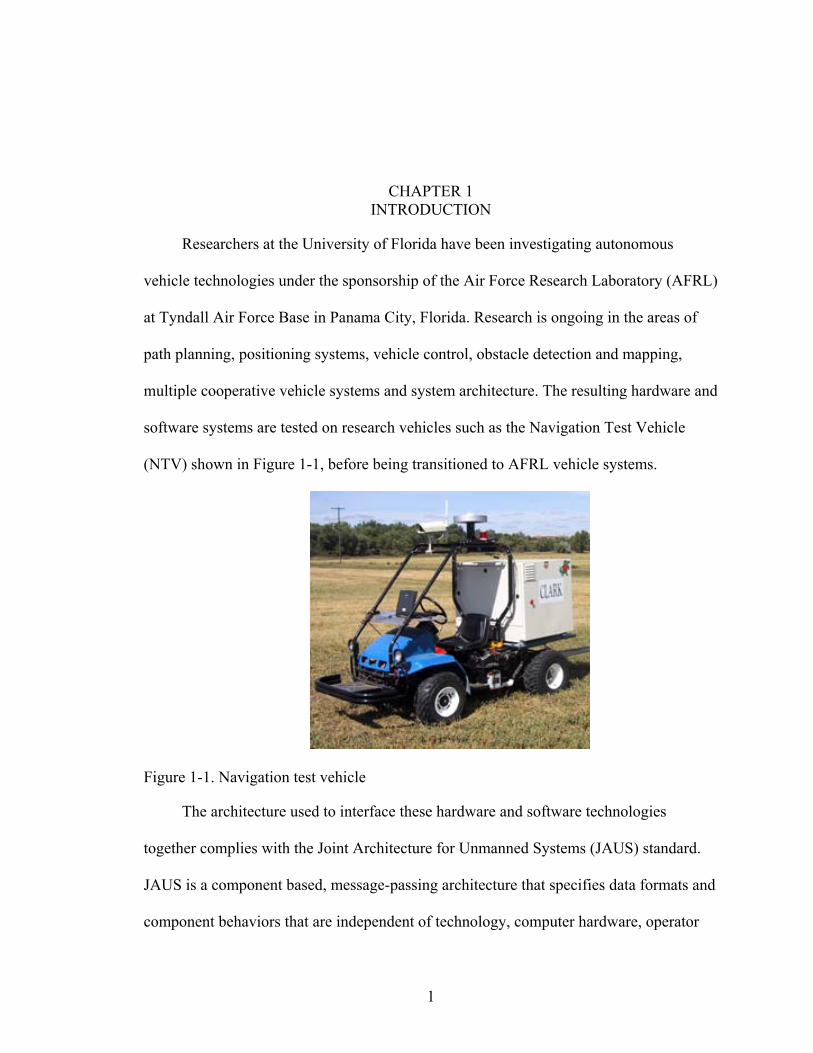
Researchers at the University of Florida have been investigating autonomous

vehicle technologies under the sponsorship of the Air Force Research Laboratory (AFRL)

at Tyndall Air Force Base in Panama City, Florida. Research is ongoing in the areas of

path planning, positioning systems, vehicle control, obstacle detection and mapping,

multiple cooperative vehicle systems and system architecture. The resulting hardware and

software systems are tested on research vehicles such as the Navigation Test Vehicle

(NTV) shown in Figure 1-1, before being transitioned to AFRL vehicle systems.

Figure 1-1. Navigation test vehicle

The architecture used to interface these hardware and software technologies

together complies with the Joint Architecture for Unmanned Systems (JAUS) standard.

JAUS is a component based, message-passing architecture that specifies data formats and

component behaviors that are independent of technology, computer hardware, operator

1

2

use, and type of vehicle platform. JAUS is designed to be used with any air, land, surface

or underwater unmanned system.

The flexibility of JAUS in regards to the vehicle platform is due to the generic

nature of the data string sent to the Primitive Driver Component. With this architecture

the vehicle is treated as a rigid body with an arbitrary system of forces and moments

acting upon it. These forces and moments yield an equivalent force and torque about the

vehicles origin that can be used to characterize the motion of the vehicle. The ability to

characterize the motion of any rigid body with six values becomes very important when

standardized messaging for all types of vehicles is needed. The equivalent set of forces

and moments that is passed to the Primitive Driver Component in this type of architecture

is known as a wrench.

The test vehicles currently used for the research and development of this system

architecture at the University of Florida are for the most part comprised of Ackerman

steered and tracked vehicles. These vehicle systems are limited in their mobility due to

the non-holonomic constraints of their wheels. In terms of the coordinate system in

Figure 1-2 these vehicles are constrained to a translation on the X-axis and a moment

about the Z-axis.

Figure 1-2. Vehicle coordinate system

3

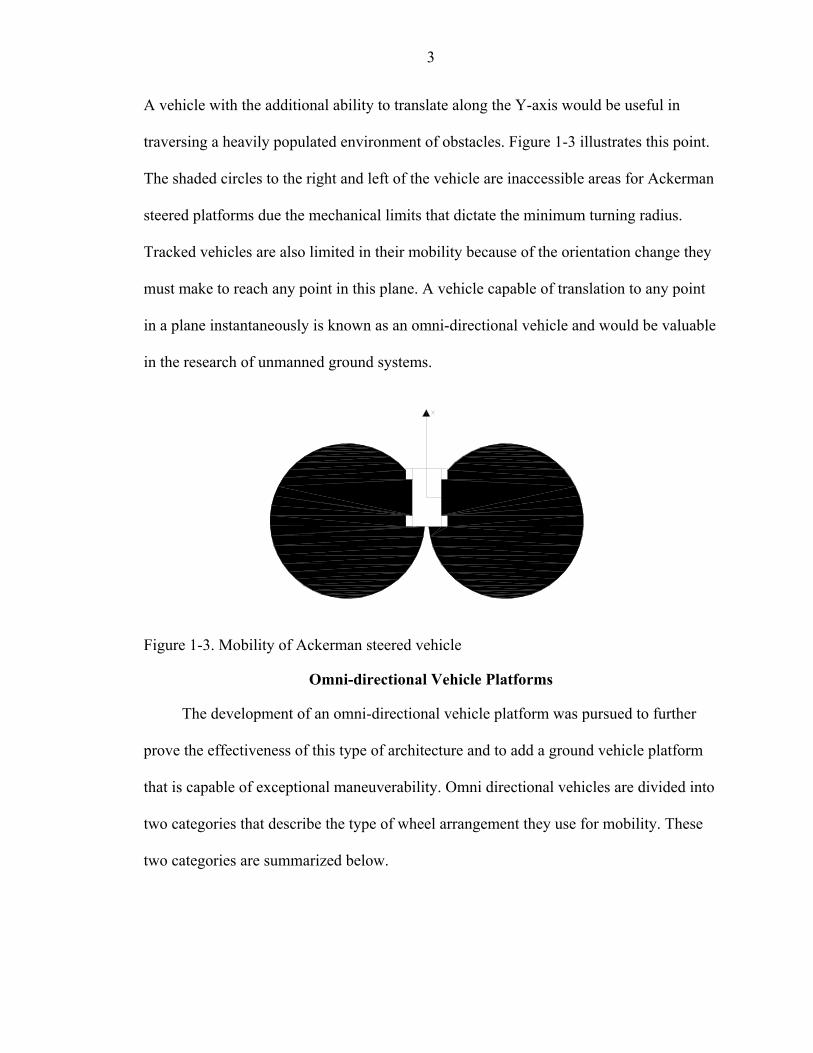
A vehicle with the additional ability to translate along the Y-axis would be useful in

traversing a heavily populated environment of obstacles. Figure 1-3 illustrates this point.

The shaded circles to the right and left of the vehicle are inaccessible areas for Ackerman

steered platforms due the mechanical limits that dictate the minimum turning radius.

Tracked vehicles are also limited in their mobility because of the orientation change they

must make to reach any point in this plane. A vehicle capable of translation to any point

in a plane instantaneously is known as an omni-directional vehicle and would be valuable

in the research of unmanned ground systems.

Figure 1-3. Mobility of Ackerman steered vehicle

Omni-directional Vehicle Platforms

The development of an omni-directional vehicle platform was pursued to further

prove the effectiveness of this type of architecture and to add a ground vehicle platform

that is capable of exceptional maneuverability. Omni directional vehicles are divided into

two categories that describe the type of wheel arrangement they use for mobility. These

two categories are summarized below.

4

Special Wheel Designs

Special wheel designs include the universal wheel, the Mecanum wheel, and the

ball wheel mechanism. The universal wheel provides a combination of constrained and

unconstrained motion during turning. The mechanism consists of small rollers located

around the outer diameter of a wheel to allow for normal wheel rotation, yet be free to

roll in the direction parallel to the wheels axis. The wheel is capable of this action

because the rollers are mounted perpendicular to the axis of rotation of the wheel. When

two or more of these wheels are mounted on a vehicle platform their combined

constrained and unconstrained motion allows for omni-directional mobility. Figure 1-4

and 1-5 illustrate the mechanics of the universal wheel and a sample platform with two

universal wheels. The traction wheel labeled (T) in the illustration is used to translate the

platform while the rudder wheel (R) is used for steering. The other two wheels mounted

parallel to the traction wheel are passive and provide platform stability.

Figure 1-4. Universal wheel (Yamashita et al., 2001)

5

Figure 1-5. Universal wheel platform

The Mecanum wheel is similar to the universal wheel in design except that its

rollers are mounted on angles as shown in Figure 1-6. This configuration transmits a

portion of the force in the rotational direction of the wheel to a force normal to the

direction of the wheel. The platform configuration consists of four wheels located

similarly to that of an automobile. The forces due to the direction and speed of each of

the four wheels can be summed into a total force vector, which allows for vehicle

translation in any direction (Diegel et al., 2000).

Figure 1-6. Mecanum wheel (Diegel et al., 2002)

Another special wheel design is the ball wheel mechanism. It uses an active ring

driven by a motor and gearbox to transmit power through rollers and via friction to a ball

that is capable of rotation in any direction instantaneously. An illustration of this type of

wheel is shown in Figure 1-7. Each of these previously mentioned designs achieve

6

excellent maneuverability, but are limited to hard even surfaces due to the small roller

diameters.

Figure 1-7. Ball wheel (Yu et al., 2000)

Conventional Wheel Designs

Conventional wheel designs have larger load capacities and a higher tolerance for

ground irregularities compared to the special wheel configurations. However, due to their

non-holonomic nature, they are not truly omni-directional wheels. These designs are not

truly omni-directional because when a move with a non-continuous curve is encountered

there is a finite amount of time before the steering motors can reorient the wheels to

match the projected curve. The time constant of this process is assumed much faster than

the gross vehicle dynamics for most applications. Therefore, it is assumed to be capable

of zero-radius trajectories and retains the term omni-directional. Most platforms that

contain conventional wheels and approximate omni-directional mobility incorporate at

least two independently steered and independently driven wheels. Active castor wheels

like the one shown in Figure 1-8 can be used to achieve this near omni-directional

mobility. An example of a platform that uses this type of wheel arrangement is given in

Figure 1-9. The platform shown in this figure was designed and built by Utah State

University and is known as Technology II. It achieves omni-directional mobility via six

independently steered and independently driven wheels.

7

Figure 1-8. Active castor wheel

Figure 1-9. Technology II (Utah State University)

Vehicle Criteria

Research in the area of highly mobile vehicle platforms that are capable of indoor

and all-terrain activities is necessary to further develop control and path planning systems

currently in use at the University of Florida. A conventional wheel arrangement with four

independently driven and independently steered wheels would provide the necessary

platform mobility to meet these research needs. The design of the drive system is critical

for this research vehicle due to the size constraints given for indoor mobility and the

power requirements needed for outdoor navigation. The focus of this paper is the design

of a motorized wheel that can meet these needs.

8

Approach

The concept is to have four drive wheels, where the commonly unused space within

the wheel hub of a wheel is used to mount a power train capable of propelling a 400 lb

vehicle at a continuous speed of 7.33 ft/sec (5mph). An overview of the technology

required to design and fabricate such a system is presented below. In the following

chapters the specifics of the design and fabrication process will be addressed. This is

concluded with a description of the method and apparatus used to test the drive unit and

the performance specifications determined from these tests.

Background

Permanent-Magnet Motors

The most fundamental decision in the design of the drive wheel is the selection of

the motor. The selection of the housings, bearings, gearing, cooling and motor control are

all contingent upon the specifications of the motor. The two distinct types of motors that

could be considered for this design are brushed and brushless permanent magnet DC

motors. A brushed motor uses a pair of brushes and a commutator to switch the polarity

of the windings in order to maintain a unidirectional torque. Some of the concerns with

these motors include wear on the brushes and arcing due to the mechanical contact

between the commutator and the brushes. This is dangerous in environments where

fumes from flammable materials could be present. Brushed motors suffer small voltage

losses due to the mechanical switching. They are also more difficult to cool in certain

situations due to the generation of heat on the rotor.

Brushless motors use power transistors to perform the polarity switching necessary

to produce a rotational motion. These switches excite the coils of the motor in

9

synchronism with rotor position. This type of motor is more costly but it is more efficient

and maintenance free and, therefore, was selected for this research.

There are three physical configurations of permanent magnet DC brushless motors.

The outer rotor configuration has a fixed armature winding on the stator with magnets

mounted to an outer disk. These motors are generally used on applications where a

constant rotational speed is desired. The large diameter rotor helps to increase the inertia

which smoothes out speed variations. Outer rotor motors are more difficult to cool than

other designs because there is very little conduction between the housing and heat-

generating armature. Axial-gap disc motors are used in applications where there is a need

for a thin low torque motor. The main advantage to this type of motor is their low cost,

their flat shape and capability for very smooth rotation. Inner rotor motors consist of a

rotating core spinning in the center of the stator. This configuration is common in servo

systems due to the low inertia of the rotor thus allowing for quicker acceleration and

deceleration. An iron core is used as a backing for the magnets. It is often enough to bond

the magnets to the iron rotor, but in some high-speed situations the interior rotor may

require a retaining can made out of stainless steel or some other high-resitivity alloy to

prevent the magnets from flying apart. Figure 1-10 illustrates the three distinct types of

brushless DC motors.

The DC brushless motor is basically a permanent magnet rotating past a series of

current-carrying conductors known as phases. Brushless motors are available in two,

three, and four phase configurations. The three phase motors are the most common and

will be discussed further. Figure 1-11 illustrates the three types of three phase designs:

delta bipolar, wye bipolar, and wye unipolar. It is shown from this figure how the

10

completion of the circuit through the transistor switches induces current flow in the

phases.

Figure 1-10. Brushless DC motor types (Hendershot and Miller, 1994)

Figure 1-11. The three types of three phase designs (BEI)

When this energizing of the phases is completed sequentially a rotational motion is

produced due to the desire of the permanent magnet to align itself with the zero torque

position. The motor is said to operate with squarewave excitation because the DC current

switches polarity in synchronism with the passage of alternate N and S magnet poles

(Hendershot and Miller). The resultant output torque of a three phase bipolar

configuration is shown in Figure 1-12.

11

Figure 1-12. Effective torque ripple, three phase bipolar (BEI)

Performance characteristics

The speed-torque curve of a motor represents the steady-state capacity of the motor

in driving various types of loads. The motor curve must be compatible with the speed

torque curve of the load to ensure that the motor has enough torque to accelerate the load

from standstill and maintain full speed without exceeding any thermal or electrical limits

(Hendershot and Miller). The thermal and electrical limits are characterized by the

boundary conditions on the curve.

When a motor rotates, a back electromotive force proportional to the speed of

rotation is produced that directly opposes the applied voltage. Equation 1-1 relates the

back-EMF ( and speed ()E )ω with the back-EMF constant ( )Ek .

ωEkE = (1-1)

The applied voltage ( in a DC motor is equal to the sum of the back-EMF and the

resistive volt-drop in the motor windings as shown in Equation 1-2.

)SV

V RIES += , (1-2)

where R is the resistance in the phases and I is the DC supply current. The maximum

speed achievable for a motor with a constant supply voltage occurs at no load. Equation

1-3 gives the no load speed ( )NLω by combining equations 1-1 and 1-2 and canceling out

12

the resistive voltage-drop due to the relationship between torque and current. The locked

rotor torque ( is calculated from Equation 1-4. The two constants used in the

following equations are given by the motor manufacture as the EMF constant and

the torque constant ( ) .

)

)

LRT

( Ek

Tk

E

SNL k

V=ω (1-3)

RV

kIkT STTLR == (1-4)

A motor speed-torque curve can be generated from the calculated values of the two

previous equations due to their approximately linear relationship. Equation 1-3 shows

that by adjusting the supply voltage to the motor the speed of the motor can be changed.

As a load torque is applied, the current draw from the supply increases thereby increasing

the resistive volt drop and decreasing the supply voltage available to the motor for

maintaining its rotational speed. This explains the linear nature of the speed-torque curve.

Figure 1-13 illustrates a sample speed-torque and power-torque curve where the

maximum power output is defined by ( )MAXP .

The ideal curve presented here cannot be obtained in a real motor but may be

closely approached. Some of the losses that contribute to the non-linearity of the speed-

torque curve include the core losses in the laminated iron, windage and bearing friction.

The ideal curve provides the maximum theoretical performance characteristics of a motor

at a constant supply voltage without taking into account any of the limiting factors such

as the temperature and current limits of the materials. Typically only 30% of the locked-

rotor torque may be obtained continuously due to these material limitations. Brief

operation is permitted at slightly higher load levels for a short period of time provided the

13

accumulated heating effect does not cause the temperature to rise above the long term

allowable temperature.

0100020003000400050006000700080009000

0 100 200 300 400 500

Torque

Spee

d

0100020003000400050006000700080009000

Pow

er

speed-torque curve

pow er-torquecurve

PmaxNo-loadspeed

PeakTorque

Figure 1-13. Permanent magnet dc motor characteristics

Cooling

Temperature limits the continuous load torque a motor is able to produce. If the

temperature rises above the allowable value the winding insulation will begin to burn off

and demagnetization of the permanent magnet will occur. Cooling increases the

performance characteristics and the life of the motor. Most designs take advantage of the

brushless motor’s ability to conduct heat between the armature and the motor housing.

Other modes of heat dissipation include natural convection and radiation. For high power

density motors an oil mist, refrigerant or liquid coolant may be used to increase the power

output without increasing the frame size. The life of the electrical insulation on the

windings of the motor can be determined through statistical methods. The relationship

between life and temperature is exponential and inversely related. For example, if the

motor maintains a sustained 50 increase in temperature the life of the motor windings F°

14

decreases by 50% (Hendershot and Miller). From this example, the importance proper

cooling and rating of the motor is shown.

Position sensing

The brushless servo amplifier controls the excitation of the phases in the motor. In

order for the amplifier to be in synchronization with the poles of the motor, the position

of the rotor must be known. The most common position sensors include the resolver,

encoder, and Hall-effect sensor. The resolver is an absolute position transducer that can

give the rotor’s position at any speed including zero. It provides a very fine resolution

shaft position signal with a two-phase (sine/cosine) curve at the rotor frequency.

Resolvers are very rugged and are similar in design to a brushless motor.

The second type of shaft position sensor is the optical encoder. Optical encoders

also provide a very fine resolution shaft position signal through the use of

phototransistors, photoemitters, and a code disk. Encoders can be purchased in both

absolute and incremental configurations. Incremental encoders generate a quadrature

output from the sensing of two out-of-phase tracks. They can only measure the relative

position of the shaft, but are useful in the velocity control of brushless motors due to their

high resolution. The absolute encoder is designed to produce a digital signal that

distinguishes N distinct positions of the shaft. This type of encoder is much more

expensive than the incremental encoder and is often unnecessary in servo applications

where a homing sequence can be performed or only relative position is needed. The Hall-

effect position sensor is the least expensive of the three sensors mentioned. This

transducer is also the simplest shaft position sensor used in the generation of

commutation pulses. A Hall switch is triggered by a magnetic field that is above a set

threshold value. A three-phase motor will contain three Hall-effect sensors spaced at

15

°60 or 120 electrical. Electrical degrees are simply mechanical degrees multiplied by the

number of pole pairs in the motor. These sensors give adequate rotor position to excite

the phases in the proper sequence.

°

Gearing

The use of gearing decreases the required motor size by converting the motor’s

high rotational speed and low torque to a torque and speed that match the load

requirements. For this application this can be accomplished through the use of harmonic

or epicyclic gearing. To simplify the drive wheel design a gearless system consisting of a

high torque, low speed motor could be employed. However, to meet the power and size

requirements it was decided to couple an epicyclic gear train to a high-speed motor.

Epicyclic gearing

Epicyclic gear trains (EGTs) are chosen for many applications due to their high

power to weight ratio. Figure 1-14 illustrates a typical EGT. EGTs are often called

planetary gear trains (PGTs) because of the orbiting motion the planet gears (elements

3,4,and 5 in Figure 1-14) have around the sun (element 1). The planets are connected by a

carrier sometimes called an arm or spider (element 7), which rotates about an axis

concentric to that of the sun and ring (element 6). Many applications make use of

multiple planets to achieve a high power to weight ratio. Power branching allows the

gears to share the tangential force evenly throughout the gear train. The advantage of this

type of arrangement is that the radial forces produced during the transmission of torque

across an involute gear pair are canceled out.

EGTs typically have a mobility of 2, which indicates that two inputs are needed to

define a unique output. For the simple case one element is fixed giving the overall ratios

16

defined in Table 1-1. Epicyclic gear trains are designed to use spur, helical, or double

helical gearing.

Figure 1-14: Epicyclic gear train spur gears

Table 1-1: Epicyclic gear arrangements (South and Mancuso, 1994) Fixed Input Output Overall Range of ratios

Arrangement Member Member Member ratio normally used

Planetary Ring Sun Carrier Nr/Ns+1 3:1 - 12:1 Star Carrier Sun Ring Nr/Ns 2:1 - 11:1 Solar Sun Ring Carrier Ns/Nr+1 1.2:1 - 1.7:1

Ns = Number of sun teeth Np = Number of planet teeth Nr = Number of Ring Teeth

Spur gears

Spur gearing is used in the transmission of power between parallel shafts.

Designers tend to use spur gears whenever application requirements permit due to their

simplicity of manufacture. Spur gears are also very tolerant to machining errors. Their

involute profile allows the center distance to change without altering the trueness of the

gear action. Spur gears are typically used in applications with pitch line velocities below

66 feet per second due to the noise generated from the teeth coming in and out of mesh.

The noise produced in gearing is a function of the speed of the gear pair. If noise were a

concern helical gearing would be a possible solution.

17

Spur gear dimensions. Spur gears are measured in the English system by their

diametral pitch, which is the number of teeth per inch of the gear pitch diameter. The

diametral pitch of a gear cannot be measured though it can be used as reference

dimension to calculate other size dimensions that are measurable. Some of these

measurable dimensions are illustrated in Figure 1-15. Most gears produced today have a

pressure angle of . Some designs incorporate or pressure angles but are not

as smooth running as the gears. In the past a 14 pressure angle was used but this

often lead to problems with undercutting. Undercutting is a concern with any pressure

angle. To reduce undercutting minimum tooth requirements must be maintained for each

of the pressure angles.

°20 °5.22

°5.

°25

°20

Figure 1-15. Spur gear terminology (Horton and Ryffel, 2000)

Table 1-2 provides an overview of involute spur gear dimensions. The equations in the

table are used to determine the manufacturing and operating dimensions of a gear pair.

18

Table 1-2. Formulas for the dimensioning of spur gears (Horton and Ryffel, 2000) Nomenclature:

φ = Pressure Angle

a = Addendum Ga = Addendum of Gear Pa = Addendum of Pinion

b = Dedendum c = Clearance C = Center Distance D = Pitch Diameter GD = Pitch Diameter of Gear PD = Pitch Diameter of Pinion

BD = Base Circle Diameter OD = Outside Diameter RD = Root Diameter

F = Face Width

kh = Working Depth of Tooth th = Whole Depth of Tooth

Gm = Gear Ratio

N = Number of Teeth GN = Number of Teeth in Gear PN = Number of Teeth in Pinion

p = Circular Pitch P = Diametral Pitch

Table 1-2 cont. Formulas for the dimensioning of spur gears (Horton and Ryffel, 2000)

Circular Pitch

Center Distance

Diametral Pitch

Gear Ratio

Addendum a = 1.000 / PDedendum (Preferred) b = 1.250 / P (Shaved or Ground Teeth) b = 1.350 / PWorking Depth 2.000 / PWhole Depth (Preferred) 2.250 / P (Shaved or Ground Teeth) 2.350 / PClearance (Preferred) c = 0.250 / P (Shaved or Ground Teeth) c = 0.350 / PPitch Diameter D = N / POutside Diameter (N+2) / PRoot Diameter (Preferred) (N-2.5) / P (Shaved or Ground Teeth) (N-2.7) / PCircular Thickness -- Basic t = 1.5708

Formulas for Dimensions of Standard Spur Gears

Formulas for Tooth Parts, 20-and 25-degree Involute Full-depth TeethANISI Coarse Pitch Spure Gear Tooth Forms

NDp π

=

PNN

C PG

2+

=

DNP =

P

GG N

Nm =

=kh

=th=th

=OD=OD=OD

Gear strength. A primary difficulty in gear design is the calculation of the gear

tooth stresses. The stresses calculated in gear design formulas are not necessarily true

19

stresses. For example, the load may be known but when this load is not uniformly

distributed across the face width the calculations only serve as an estimate in determining

the design parameters. Errors in tooth spacing also contribute to higher loads than

expected. The accelerations and decelerations of a gear due to these errors cause dynamic

overloads that cannot be accurately modeled in simple design formulas. Despite these

problems, gear stress formulas can approximate the performance of a new gear design. A

modified Lewis equation is defined in Equation 1-5. It assumes the load application at the

tip of the tooth, even though this is an approximation because more than one tooth is in

contact at any one time.

wYkPF

d

t=σ , (1-5)

where σ = Stress, lb 2/ in

tF = Tangential force, lbs

P = Diametral pitch, 1 in/

w = Face width, in

Y = Lewis form factor (Horton and Ryffel, 2000)

dk = Barth speed factor

The Barth speed factor is defined in the following equation. It partially accounts for the

kinetic loading effects on the gear pair.

rd va

ak+

= , (1-6)

where v = Pitch circle velocity, feet per minute (fpm) r

a = 600 for ordinary industrial gears and 1200 for precision cut gears

20

Lubrication. Lubrication is required in order to limit metal-to-metal contact

between two gear surfaces. Inadequate lubrication can lead to the scoring and pitting of

gear teeth. When designing a gear train for the transmission of power through the

analysis of gear, shaft, and bearing capacities it is also necessary to analyze the thermal

limits of the gearbox. Most small gear drives are splashed lubricated by a quantity of oil

in the gearbox. The surrounding air cools the gearbox and lubricant without the help of a

pump and heat exchanger. A common practice is to calculate the maximum power a

gearbox can carry for 3 hours without the oil temperature exceeding while having

an ambient temperature of less than 100 .

F°200

CHAPTER 2 MOTOR AND GEAR TRAIN DESIGN

Load

Before completing the drive wheel design the load requirements must be

determined. The torque output required for each of the four wheels on the omni-

directional vehicle was found through empirical methods. The torque cannot be estimated

by theoretical means due to the complexity of the tire ground contact and the

corresponding rolling resistance. Because the rolling resistance is highly dependent on

the tire dimensions, the tire inflation pressure and the ground characteristics, the load test

was completed with similar values for each of these variables. Table 2-1 gives the values

found for the load test.

Table 2-1. Thrust needed to translate a 400lb vehicle Concrete 45 lbLevel grass 60 lbGrass with 10 deg. Incline 130 lbGrass with 20 deg. Incline 197 lb

Motor Selection

Motor selection for the drive wheel is based on the characteristics of the

mechanical system coupled to the motor shaft. The combined selection of the motor and

gear train is a highly iterative process. The final estimated values for the drive wheel are

used to demonstrate the motor selection equations. The final design specifications are

given in Table 2-2 along with the estimates for the physical properties of the mechanical

system.

21

22

Table 2-2. Estimates for the physical properties of the wheel Load Vehicle weight 400 lb Rated speed of operation 5 mph Equivalent Inertia* 0.166 in-oz-sec^2 Rated acceleration* 444.7 rad/sec^2Tire size 4.10 - 3.50 - 6 Outer diameter 12.1 inch Inner diameter 6 inch Width 3.5 inchGear Box Reduction 30.333 Inertia estimate* 0.12 in-oz-sec^2 Efficiency 90 % Frictional torque estimate* 27 in-ozMotor DIP37-19-005Z DC Resistance 0.25 Ohms Torque sensitivity 10.6 oz-in/Amp Back EMF constant 0.075 Volts/(rad/sec) Peak torque 400 in-oz Continuous stall torque 120 in-oz Max Speed 8000 rpm

* Values taken at motor shaft

Selecting the right motor for an application requires knowledge of the peak torque

requirement, RMS torque requirement, and the speed of operation. The peak torque ( )PT

is the sum of the torque used to accelerate the inertia of the system , the torque to

move the load ( , and the torque to overcome friction

( JT )

)LT ( )FT . This relationship is given

in Equation 2-1.

FLJP TTTT ++= (2-1)

The torque required to accelerate the vehicle is a product of the inertia of the load

and the load acceleration ( MLJ + ) ( )α as given in Equation 2-2. The inertia in the system

is the sum of the inertia of the rotating bodies in the wheel and the equivalent inertia of

the vehicle relative to its mass and wheel diameter. From these calculations the peak

23

motor torque required to accelerate the vehicle at a rate of 7 is 258 in-oz. The

load and motor inertia are given in Table 2-2.

2sec/33. ft

32) tF

α⋅= +MLJ JT (2-2)

The Root-Mean-Square (RMS) torque is a value used to approximate the average

continuous torque requirement. It is a statistical approximation defined by Equation 2-3.

The traction type loading of the vehicle requires a constant torque over a prescribed speed

range, so for this application the vehicle is assumed to operate at a constant speed.

Therefore, the RMS torque is assumed to be equal to the sum of the torque needed to

move the load and the torque required to overcome friction. The RMS torque is

calculated to be 130 in-oz.

4321

22

12 ()(

ttttTTTtTTtT

T LJFLPRMS +++

−−+++= (2-3)

where =t Acceleration time, sec. 1

Dwell time, sec. =2t

Deceleration time, sec. =3t

Off time, sec. =4t

A motor candidate was selected according to the previous calculations and the

known size constraints. The motor specifications required to complete the analysis are

given in Table 2-2 and an extended list of these specifications is given in Appendix A

with the motor drawing. The next step in the verification of the motor for the drive wheel

was to analyze the motor winding parameters. The supply voltage available on the

vehicle is rated at 48 volts. The voltage drop due to the speed of the motor and the

corresponding back EMF is defined in Equation 2-4. The voltage found from Equation 2-

24

4 is used to determine the available current to produce torque. The current is equal to the

voltage divided by the motor winding resistance.

ωESOURCE kVV −= (2-4)

where =k Back EMF constant, E Ampozin /−

=ω Rotational speed of the motor shaft, rad/sec

From these calculations the voltage available to produce torque during 7.33 ft /sec (5

mph) operation of the vehicle is 15 V. The available current to produce torque is then

found to be 60 Amps. The current required by the load is defined by Equation 2-5 where

is the torque sensitivity constant. From these calculations, the current required for the

RMS torque is 12.26 amps and the current required for the peak torque is 24.34 amps

thus making this motor winding a good match for the drive wheel.

tK

t

S KTI = (2-5)

Controller Selection

A brushless DC servo amplifier is used to drive the brushless motor at a high

switching frequency. The amplifier excites the coils of the motor in synchronism with

rotor position. The rotor position is commutated to the amplifier through the Hall-effect

sensors built into the motor and a 1000 count encoder housed within the drive wheel. The

drive wheel needs the encoder for velocity control and to decrease the torque ripple

(cogging) at low speeds. These requirements along with the motor current and voltage

requirements are used to select an amplifier for the system. The amplifier selected for the

control of the drive wheel is model number BE40A8 that is produced by Advance Motion

Controls. The amplifier has an operating voltage range of 20 – 80 Volts, a continuous

25

supply current of 20 amps and a peak supply current of 40 amps. The current available to

the motor can be adjusted on the amplifier to prevent motor damage. From this

performance criterion it is shown that the amplifier meets the needs of the system.

Gear Train Design

Incorporated within the iterative motor selection process is the design of the gear

train. An exhaustive search methodology was used to optimize the gear train to meet the

size constraints and load capacities. Figure 2-1 depicts the schematic of the double stage

epicyclic gear train designed for the drive wheels.

Figure 2-1. Gear train torque path schematic

The first gearing stage is a planetary arrangement where the ring gear is fixed to ground

and the sun and carrier are the input and output respectively. The ratio for the first stage

is 4.67:1. The carrier from the first stage drives the sun gear for the second stage. This is

a one-piece unit allowing for a reliable transfer of power between the two stages of

gearing. The second stage is of the star configuration with a ratio of 6.50:1. The final

26

ratio of the dual epicyclic gear train is 30.3:1 allowing for 5 mph operation of the vehicle

with a motor speed of 4250 rev/min. Table 2-3 and Table 2-4 give the manufacturing data

for the two stages of gearing. The complete table of gear specifications is given in

Appendix B and dimensioned drawings for the gears can be found in Appendix A. This

data was acquired from the equations presented in Chapter 1.

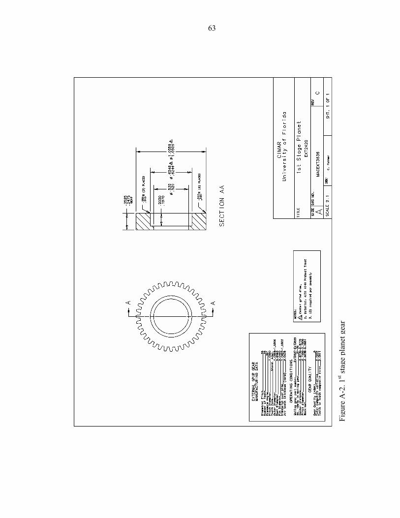
Table 2-3. Manufacturing data for the 1st stage planetary arrangement

Mesh 1 Mesh 2Sun Planets Ring

EXT3627 EXT3636 INT3699

Diametral Pitch 36 36 36Number of Teeth 27 36 99Pressure Angle 20 20 20Pitch Diameter 0.75 1 2.75Tooth Form Stand. Aden. Stand. Aden. Stand. Aden.Outer / Inner diameter 0.8056 0.8006 1.0556 1.0506 2.6944 2.6994Root Diameter 0.6793 0.9293 2.8207Pin Diameter 0.0480 0.0480 0.0400Dimension over pins 0.8105 0.8085 1.0622 1.0602 2.7176 2.7196Arc tooth thickness (norm) 0.0436 0.0436 0.0436

1st Stage Planetary Arrangement

Manufacturing Data

Due to constraints, the first stage epicyclic gearing has a non-standard diametral

pitch of 36 teeth/in. The second stage of the gear train has a diametral pitch of 24 teeth/in.

The selection of the pitch and the pitch diameter of each gear are critical. To assemble

each gear set Equation 2-6 has to hold true.

PSr NNN 2+= (2-6)

where Number of teeth on the sun gear =SN

Number of teeth on the planet gear =PN

Number of teeth on the ring gear =rN

27

Table 2-4. Manufacturing data for the 2nd stage planetary arrangement

Mesh 1 Mesh 2Sun Planets Ring

EXT2420 EXT2455 INT24130

Diametral Pitch 24 24 24Number of Teeth 20 55 130Pressure Angle 20 20 20Pitch Diameter 0.8333 2.2917 5.4167Tooth Form Stand. Aden. Stand. Aden. Stand. Aden.Outer / Inner diameter 0.9167 0.9117 2.3750 2.3700 5.3333 5.3383Root Diameter 0.7293 2.1877 5.5207Pin Diameter 0.0720 0.0720 0.0600Dimension over pins 0.9269 0.9249 2.3861 2.3841 5.3618 5.3620Arc tooth thickness (norm) 0.0655 0.0655 0.0655

2nd Stage planetary arrangement

Manufacturing Data

To evenly distribute multiple planet gears around the periphery of the sun gear, the

selection of the number of teeth on the ring, sun, and planet gears is not arbitrary (Dooner

and Seireg). Equation 2-7 is used to evenly space the planets around sun gear where n is

the number of planets in the epicyclic gear train.

IntegernNN Sr =

+ (2-7)

The modified Lewis equations presented in Chapter 1 were used to find the

maximum allowable tooth load for each the gears. A factor of safety of 3 was used in the

computation of the gear dimensions to account for the machining inaccuracies and

dynamic overloading present in the system.

Gear Backlash

Backlash is designed into the gear train to compensate for machining inaccuracies and

thermal expansion. Backlash is the play between mating teeth and is measured as the

amount of excess space between the tooth and the width of the tooth space of the

engaging gear on the pitch circle. Backlash prevents the jamming of gear teeth and

provides space for lubrication, which prevents overloading, overheating, and excessive

28

wear. The calculation of the center distance tolerance for the two epicyclic gear trains

was very important in the design of the drive wheel. The inaccuracies due to shaft,

bearing, and gear tolerances and their machining allowances were taken into account for

each gear mesh. The gear profile inaccuracies and the thermal expansion of the gears

were also taken into account to determine the amount of desired backlash. The

breakdown of the inaccuracies accounted for in the backlash calculations is given in

Appendix B.

Bearing Life

The planet bearings for the first and second stages of gearing are analyzed throughout

the design iteration to determine their expected operating life. The life of a bearing

refers to the life associated with 90% reliability and is defined in Equation 2-8.

10L

3

10

=PCL , (2-8)

where Life of the bearing in millions of revolutions =10L

C = Basic load rating, lb. (provided by bearing manufacture)

P = Equivalent radial load, lb

From Equation 2-8 it was found that all of the bearings within the gear train of the drive

wheel would exceed 50,000 hours of operation. The life of these bearings is high due to

the low radial loads produced by the planetary gearing. The planet bearings are used for

the calculations due to the load they carry for the transmission of torque.

Motor Cooling

Increasing the power density of the motor can be accomplished through the use of

forced cooling. Due to the sealed nature of the drive wheel the motor is unable to be

29

cooled by forced air. The motor housing contains 18 passages that circulate an ethylene

glycol and water mixture around the outer diameter of the stator. These passages yield

about 25 square inches of cooling area allowing for continuous duty operation at higher

torque levels than previously calculated. The coolant flows through each of the individual

drive hubs using a central pump and heat exchanger. The temperature of the motor

windings is continually monitored with a thermistor that is epoxied to the motor windings

with a thermally conductive epoxy.

The motor housing drawings depicting the coolant paths are given in Appendix A.

From the dimensions of the coolant path the maximum flow rate for laminar flow, the

pressure loss and the power dissipated are estimated.

Gearing Features

Throughout the gear train there are many unique features that allow the drive train

to fit within the hub of a wheel. Some of the features are illustrated below. Figure 2-2

illustrates the first stage sun gear and the motor shaft integrated as one unit. The slots in

the shaft act as an internal collet for joining the motor rotor and shaft. As the expanding

pin is threaded into the end of the shaft, the shaft expands creating an interference fit with

the rotor. Figure 2-3 illustrates the first stage carrier and the second stage sun gear

integrated as one unit to provide a reliable transfer of power between the two stages.

Figure 2-4 shows the first stage ring gear integrated as a part of the gear housing. Notice

the tooth relief groove separating the inner face of the housing and the ring gear teeth.

On the reverse side of this gear is a seal surface to keep the gear oil within the confines of

the gear train.

30

Figure 2-2. Main shaft and its expanding collet

Figure 2-3. First stage planets and second stage sun gear

Figure 2-4. First stage ring gear

31

Figure 2-5 depicts the second stage sun and planet gears. The planets are supported

by a fixed carrier, which is attached to the first stage ring gear.

Figure 2-5. Second stage gearing

CHAPTER 3 DRIVE WHEEL HOUSING AND JOINT DESIGN

Load Considerations

The tire is subjected to external forces due to the relative motion of the vehicle and

its weight. To determine if these loads cause failure within the design of the drive wheel

the maximum forces must be found. The forces the tire resists and their respective

directions are shown in Figure 3-1. The forces are assumed to load the tire at the center of

the tire contact area with the ground. The moment in Figure 3-1 is given as the

maximum turning moment needed to overcome the force distribution restricting the

wheel’s rotation about the z-axis. The reaction forces from the wheel clamp are also

shown in the figure and all are assumed positive.

zGM

Figure 3-1. Drive wheel ground contact forces

32

33

The vehicle is assumed to be a maximum of 400 lbs of equally distributed weight

as given by the design criteria. The maximum weight ( )W each wheel is assumed to

support is 150 lbs to account for the pitch and roll of the vehicle on inclines and in turns.

A maximum coefficient of friction ( )µ value of 0.8 is also assumed, therefore ( )W⋅µ is

the maximum force attainable in the XY plane. The loading on point G in Figure 3-1 is

used to obtain the 3 reaction forces and 3 reaction moments resulting from the wheel

clamp at point A. These reaction forces are then used to determine the forces placed on

the main bearings supporting the external wheel hub. The free body diagram in Figure 3-

2 was used to derive Equations 3-1 through 3-4. These equations describe the loading on

points B and C in the figure.

Figure 3-2. Free body diagram of the drive train

2

1

lRlMRF xAzA

xAxB⋅−

+−= (3-1)

2

21

llRlRM

F xAzAxAzB

⋅+⋅+−= (3-2)

2

1

lRlM

F xAzAxC

⋅−= (3-3)

34

2

21

llRlRM

RF zAzAxAxAzC

⋅+⋅++−= (3-4)

Due to the design of the housings and shaft that support bearings B and C, only one

bearing at a time can carry the force on the Y-axis. Bearing C carries the full load in the

Y direction if and the opposite is true when the reaction force . 0>yAR 0<yAR

In order to estimate the life of the main bearings and predict their failure the

maximum forces they experience must be calculated. The drive hub is designed to use

Reali-Slim bearings manufactured by Kaydon. The technical drawing of the bearings can

be found in Appendix A. The load capacity in the radial direction is lower than that of the

capacity in the axial direction of the selected bearings so, a function is created to

maximize the magnitude of the force exerted in the radial direction on bearing B. It was

found that the loading on bearing B would be greater than on C. The constraint was given

that the magnitude of the forces in the XY plane must not exceed ( )W⋅µ . The

magnitude of the forces in the X and Z direction and the force in the Y direction could

then be used to estimate the dynamic life of the bearings. Values obtained from the search

function are shown in Table 3-1. Knowledge of the exerted loads on the main bearings

allows the support housings that enclose the gears and motor to be analyzed for failure.

Figure 3-3 shows the complete assembly of the support housings and its related

components. The assembly in the figure is analyzed as a rigidly supported beam with two

load points. The internal shear and moment loads are determined for each point along the

Y-axis where a possibility of failure could occur.

35

Table 3-1. Maximum forces attainable for the wheel main bearings Fxg = -28.4609 lbs Fyg = -101.069 lbs Fzg = 150 lbs Rxa = 28.46095 lbs Rya = 101.0692 lbs Rza = -150 lbs Mxa = -172.915 in-lbs Mya = 170.7657 in-lbs Mza = -397.748 in-lbs Fxb = -106.155 lbs Fyb = 0 lbs Fzb = 202.3055 lbs Fxc = 77.69397 lbs Fyc = 101.0692 lbs Fzc = -52.3055 lbs

Figure 3-3. Internal drive train housings

Joints

The drive wheel joints are designed to carry the shear forces without placing a

significant amount of shear stress on the threaded fasteners. Each part contains features to

36

locate the mating part within the correct tolerances. This is critical in the design process

due to the integration of the motor, gear train and related housings. These features are

toleranced to allow for acceptable clearances throughout the operating temperature range

and to have the ability to be produced by conventional machining practices.

The threaded fasteners in the joints are assumed to only carry a tensile force due to

the moments about the X and Z-axes. The internal forces within the joint are treated like

those of a prismatic beam in bending. This approximation is assumed due to the

significant preload that is applied to the screws. Figure 3-4 illustrates the second stage

carrier cover and the forces internal to the joint. Only the reactions due to the moment

produced by the positive force in the Z-axis direction are shown in this figure.

Figure 3-4. Carrier cover joint loading

The center of gravity of the fastener group determines the neutral axis. Tension due to the

load state plus preload is seen in the bottom bolts while fastener preload is the only force

present in the top bolts. Equation 3-5 is used to determine the forces imposed upon the

bolts with the knowledge of the moments.

37

( ) ( )∑∑ ==

⋅+

⋅= n

i zi

zixn

i xi

xizi

rrM

rrM

P1

21

2, (3-5)

where and are the distances from the centerline of the plate to the center of the

threaded fastener parallel to their respective axes, is the force that the threaded

fastener supports, and M and are the moments about the X and Z-axes. Equation 3-

5 was optimized for each joint resulting in the maximum attainable load for each screw.

xir zir

iP ( )thi

x zM

Socket head bolts were used in the design of this drive wheel due to the ability to

counter bore the head of the fastener in the housing with minimal material removal. To

determine the ideal bolts for each of the joints, the suggested preload for the fastener size

is calculated. Equation 3-6 can be used to calculate these values for reusable connections.

pti SAF ⋅⋅= 75.0 (Horton and Ryffel, 2000) (3-6)

In the previous formula, is the bolt preload, is the tensile stress area of the

bolt, and S is the proof strength of the bolt. The variable is determined through the

use of screw thread tables located in most design handbooks. Proof strength for

commonly used fasteners can also be obtained from this reference, but for the socket

head bolts in use throughout this design, an approximation had to be made with Equation

3-7 where is the yield strength of the material.

iF tA

p

S

tA

y

(Horton and Ryffel, 2000) (3-7) yp SS ⋅= 85.0

Bolt preloads are desired in loaded joints due to their ability to keep the bolts tight,

increase joint strength, to create friction between parts to resist shear, and to improve the

fatigue resistance of the bolted connection. Equation 3-8 is used to estimate the torque for

tightening the fasteners to achieve this recommended preload.

38

dPKT i ⋅⋅= (3-8)

In this equation T is the wrench torque, K is the constant that depends on bolt

material and size, is the bolt preload and is the nominal bolt diameter. A value of

0.2 is used for

iP d

K (Horton and Ryffel, 2000).

Many of the joints use internal threads. Therefore knowledge of the strength of

these internal threads is of importance. It is more desirable to have an externally threaded

member fail than an internally threaded member. To prevent stripping of the internal

threads, the minimum length of engagement of the fastener must be calculated. These

calculations are not presented here, but when carrying them out dissimilar thread

materials must be accounted for to achieve an accurate value.

The joint between the first stage ring gear and motor housing contains a fiber

gasket to prevent oil from seeping beyond the seal plate. This joint is analyzed for bolt

strength as well but extended calculations are performed to analyze the failure modes of

the gasket. The gasket stiffness and the relative stiffness of the housings and threaded

fasteners are used to analyze the joint to prevent joint separation. The effective gasket

pressures are also determined to prevent gasket crushing and leaking.

CHAPTER 4 PERFORMANCE TESTING

The drive wheel was tested to gain further understanding of the concepts presented

in the previous chapters and to verify the design for the use of vehicle propulsion in an

omni-directional vehicle. At the time of this writing, only one drive wheel has been

fabricated, thus the wheel cannot be tested on the vehicle platform. Instead testing took

place on a bench dynamometer in a controlled environment. This chapter describes the

test equipment that was built to evaluate the performance characteristics of the drive

wheel.

The wheel was load tested similarly to the way it would be used on a vehicle

platform. A brake that allows the wheel to continue to rotate while applying a variable

resistive torque is used to simulate varying terrain conditions. This resistive torque is

logged along with the current draw on the motor, the speed of the motor, and the motor

winding temperature. To gain an understanding of the effect of forced cooling on the

motor, temperature sensors are located in the coolant inlet and coolant discharge lines.

This data is logged with the motor conditions and the room temperature to provide

performance statistics on the drive wheel. In the following sections the equipment used to

test the drive wheel will be described in further detail.

Dynamometer

In order to simulate the vehicle on the test bench, an arm that constrains the motion of the

wheel to a rotation about its axis and a linear motion that is approximately vertical is

used. The arm is sprung to force the tire into contact with the dynamometer roller. The

39

40

roller used for the testing is a solid steel mass 4.9 inches in diameter and 10 inches in

length. The large inertia of this roller effectively smoothes out torque variations in the

wheel. The roller then transmits the power from the wheel through a flexible coupling

and then to the variable braking system. The braking system for this dynamometer uses

an Ingersoll-Rand 7808-B pneumatic motor that was originally designed for industrial

manufacturing processes. This type of braking system is not common in dynamometers

but was used for this application because of its availability and cost. Dynamometers

typically use some type of hydrodynamic brake, friction brake or induction motor to

provide the resistive torque needed to load the test motor. These brakes dissipate power

by dissipating energy in the form of heat. Hydrodynamic systems get rid of this heat by

circulating the fluid through a reservoir and heat exchanger circuit. Heat removal for the

pneumatic motor is not quite as simple. The pneumatic motor used for the testing of the

wheel is back driven against the air pressure to provide a braking torque. An increase in

the air supply pressure proportionally increases the torque required to back drive the

motor. This type of braking system, however, does not remove the generated heat as well

as the fluid systems due to the differences in specific heats of the fluids. A set of fins was

attached to the air motor to help dissipate the heat generated within the motor housing.

The fins also act as a reservoir for bathing the motor in ice during load testing. A pan

with a drain was placed under the air motor to catch the water runoff.

Recording the amount of braking torque applied to the test motor can be

accomplished in different ways. The most common way is to support the brake by two

bearings, allowing it to freely rotate about its axis. A load-measuring device is then

placed between the brake support and ground to resist the rotation of the brake. This

41

device can be a torsion load cell or a linear load cell coupled to a moment arm off of the

brake support. For the dynamometer built to test the drive wheel, a linear tension spring

was attached between a torque reaction arm and a ground support. A potentiometer was

then used to measure the angular displacement of the brake. Calibration was necessary

for this type of load sensing system. The dynamometer was calibrated using a ratcheting

moment arm and a series of weights to develop a polynomial expression to relate the

voltage output of the potentiometer and the resistive torque placed on the wheel. The

conditions remained the same throughout the three calibration sequences except for the

order of the applied weights. Figure 4-1 illustrates the three calibration curves describing

the voltage torque relationship. The bench dynamometer is illustrated in Figure 4-2.

y = -254.29x2 + 696.43x + 9.2986

0

50

100

150

200

250

300

350

0 0.1 0.2 0.3 0.4 0.5 0.6

Voltage (Volts)

Torq

ue (i

n-lb

)

Calibration 1Calibration 2Calibration 3Poly. (Calibration 1)

Figure 4-1. Dynamometer calibration curves

42

Figure 4-2. Bench dynamometer

Cooling

A cooling unit was built to circulate an ethylene glycol and water mixture through

the drive wheel and heat exchanger. The cooling panel, shown in Figure 4-3, consists of a

pump, heat exchanger, cooling fan, flow meter, pressure gauge, and valve for flow

control. The components used in the cooling unit are not necessarily the optimum for the

application. They simply provided the necessary cooling for the benchmarking of the

drive wheel and were used due to their availability. To determine the heat dissipated

through the liquid cooling system the inlet and discharge coolant lines of the wheel were

fitted with thermistors. These temperatures were logged along with the temperature of the

room and motor windings to see the effects of varying the torque, speed, and coolant flow

rate.

43

Figure 4-3. Coolant panel

Data Acquisition

Voltages from the health sensors on the motor were acquired through digital data

acquisition equipment and converted into the units for each of the sensors. LabView was

used to convert and display the data from each of the sensors and append it to a

spreadsheet file specific to the test run. It was set up to acquire data at a rate of 10 Hz or

120 Hz depending on the type of test.

The brushless servo amplifier has signal output pins to monitor the speed of the

motor, the supply current sent to the motor, and the fault state of the system. These

voltages were run directly into the data acquisition board without any prior conditioning.

The velocity output from the amplifier is internally isolated, however the current output is

not isolated and requires data averaging to achieve a clean value. The thermistors are

wired with a shielded twisted pair and conditioned with a capacitor prior to acquisition to

44

cancel out the interference from the mechanical and electrical systems they monitor. The

potentiometer used for torque measurement was powered by a constant 5 Volt supply and

is wired as a voltage divider. Figure 4-4 illustrates the brushless servo amplifier,

thermistor power and conditioning board and the breakout box for the data acquisition.

The complete test system schematic is illustrated below in Figure 4-5.

Figure 4-4. Amplifier and signal conditioning board

45

Figure 4-5. Testing schematic

CHAPTER 5 RESULTS

Many performance issues have been detailed in the previous chapters to provide

justification for the drive wheel design. The performance of the fabricated wheel will be

presented in this chapter to evaluate the design decisions. In these performance tests the

continuous torque, acceleration, efficiency, and general temperature constants of the

wheel will be determined. Finally the wheel constants will be summarized to give the

relevant specifications required to control and apply the wheel to any vehicle platform.

Speed/Torque Curves and Load Testing

Studying the speed/torque curves is the best way to gain an understanding of a

brushless DC motor. The motor’s capabilities for various loading conditions are acquired

from this curve. As mentioned previously, it is necessary to match the speed/torque curve

of a motor to that of the load to obtain optimum performance in the system. The

speed/torque curve ensures that the motor is capable of accelerating a load from zero

speed to full speed without exceeding any thermal, mechanical, or electrical limits

(Hendershot and Miller, 1994). These limits are characterized by the boundary of regions

on the speed/torque curve.

It was mentioned in Chapter 2 that a traction type loading, like that of the drive

wheel, requires a constant torque over a prescribed speed range. The drive wheel was

load tested on a dynamometer in order to obtain the speed/torque curve needed to

compare to the load requirements but due to the design of the air braking system on the

dynamometer a constant torque test over the full speed range was impossible. At low

46

47

speeds, the braking force of the air motor pulses in succession with the vanes loading and

unloading. In a typical application for the drive wheel the controller operates in closed

loop mode to maintain a constant commanded velocity. This system was used to achieve

a speed/torque curve for a constant velocity that could be compared to the constant torque

curve of the load. Figure 5-1 illustrates the speed vs. torque curve for the drive wheel and

the estimated criteria to maneuver a 400lb vehicle over a series of terrain conditions.

These plots were overlaid to show the compatibility of the drive wheel and the given load

criteria. The continuous load criterion is met throughout the various load conditions. It is

only when an incline in excess of 15 is encountered that the speed drops below the

designed speed. The supply voltage to the system for this test is 48 Volts. The drop in

speed at 230 in-lbs of torque could be overcome by increasing the supply voltage. The

motor winding temperature was closely monitored throughout this test to ensure that the

thermal limits of the motor were not exceeded.

°

For completeness the drive wheel was also tested with a constant voltage supply to

show the speed/torque linearity commonly provided in most suppliers’ catalogs. The test

was performed at 50% of the rated voltage for the wheel as proof of the equations defined

in Chapter 1. This curve and the related current-torque curve are given in Figure 5-2.

Maximum Continuous Torque Testing

A load test was completed for an extended amount of time to determine the

maximum continuous torque the wheel is capable of producing. Data was gathered for a

period of 70 minutes from the various health sensors on the motor and controller as the

wheel was loaded. The loading was performed in a stepping method during the search for

the maximum continuous torque. The motor winding temperature was allowed to reach a

near steady state value before the next load step was performed. This is because, for this

48

application, the maximum allowable winding temperature given by the motor

manufacture limits the continuous torque. The data points from the test are plotted in

Figure 5-3.

Figure 5-1. Speed/Torque curves for drive motor and load

Figure 5-2. Speed/Torque with a constant voltage supply 50% of the rated voltage

49

Figure 5-3. Maximum continuous torque test

Figure 5-3 is divided into seven regions corresponding to seven different coolant

flow rates. Each region’s relevant data is given in Table 5-1 for comparison. This data

shows how decreasing the coolant flow rate increases the change in temperature between

the coolant inlet and discharge. As this difference becomes larger, the motor housing

temperature increases thus lowering the maximum continuous torque. A value of 1200

cubic centimeters per minute (CCM) was chosen as the maximum tested coolant flow

rate because it efficiently yielded the desired change in temperature of 5 . After this

test was completed the gear lubricant temperature was measured to be 109 .

°F

To test the effectiveness of the external cooling system for the wheel the maximum

continuous torque was found for no coolant flow. Figure 5-4 plots the data points

gathered during the test run. The continuous allowable torque generation by the wheel

without forced cooling is limited to 170 lbin ⋅ . The liquid cooling increases the allowable

output torque by 60% thus making this design an effective way of increasing the power

50

density of the drive system. The gear train lubricant temperature was measured after this

test as well and was found to be 150 . The difference of 41 between the two tests

shows the effectiveness of liquid cooling the motor to decrease the gear train temperature.

F° F°

Table 5-1. Steady state averages for continuous torque test. Average Steady State Values I II III IV V VI VII

Flow Rate (CCM) 1200 900 700 400 200 500 1200 Current (Amps) 18.21 18.08 17.92 *** 17.17 *** *** Speed (rpm) 127.52 127.15 126.72 *** 126.51 *** *** Torque (in-lb) 287.54 286.71 284.21 *** 273.27 *** *** Motor Winding Temp. (deg. F) 257.58 257.27 258.36 *** 256.57 *** *** Coolant Inlet Temp. (deg. F) 85.29 85.50 85.26 *** 81.66 *** *** Coolant Discharge Temp. (deg. F) 90.44 91.60 93.94 *** 104.85 *** *** Delta Coolant Temp. (deg. F) 5.14 6.10 8.69 *** 23.18 *** *** Room Temp. (deg. F) 76.60 76.58 76.90 *** 77.40 *** *** *** Did Not Reach Steady State

0

50

100

150

200

250

300

350

0 500 1000 1500 2000 2500 3000 3500

Time (sec)

Current (Amps) Speed (rpm)

Torque (in-lb) Motor Winding Temp. (deg. F)

Room Temp. (deg. F)

Figure 5-4. Continuous torque without forced cooling

51

Acceleration

The mass and inertia of the vehicle and drive components dictate the rate at which

the platform can accelerate and decelerate. To determine the theoretical acceleration of

the vehicle, the inertia of the wheel and the torque required to overcome friction must be

computed. A series of acceleration tests were conducted to acquire these values from the

physical system. The tests measured the acceleration of the wheel for ten different output

torques. The current available for the motor to accelerate the wheel was limited through

the use of the current limit potentiometer on the brushless servo amplifier. Varying the

supply current to the motor proportionally changed the torque the motor produced. Three

step functions were sent to the controller for each of the ten different potentiometer

values. This data was then analyzed to determine the average acceleration, deceleration

and corresponding torque for each step. The first five of these acceleration tests are

plotted in Figures 5-5 – 5-9. The relevant torque and acceleration data is also given in

each figure. The figures are listed in the order of minimum to maximum tested

acceleration.

-50

0

50

100

150

200

250

0 2 4 6 8 10 12 14 16 18 20

Time (sec)

Spee

d (r

pm)

-8

-6

-4

-2

0

2

4

6

Cur

rent

(Am

ps)

I

Acceleration = 23.25 rad/sec^2Torque = 91.7 in-lb

Deceleration = -46.50 rad/sec^2Torque = -52.1 in-lb

II

Acceleration = 23.25 rad/sec^2Torque = 90.7 in-lb

Deceleration = -52.15 rad/sec^2Torque = -48.9 in-lb

III

Acceleration = 23.88 rad/sec^2Torque = 92.1 in-lb

Deceleration = -45.24 rad/sec^2Torque = -53.2 in-lb

I II III

CURRENT

SPEED

Figure 5-5. Speed-time, current-time plot #1

52

-50

0

50

100

150

200

250

0 2 4 6 8 10 12 14 16 18 20

Time (sec)

Spee

d (r

pm)

-10-8-6-4-20246810

Cur

rent

(Am

ps)

I II III

I

Acceleration = 37.07 rad/sec^2Torque = 118.4 in-lb

Deceleration = -60.31 rad/sec^2Torque = -87.7 in-lb

II

Acceleration = 37.07 rad/sec^2Torque = 121.0 in-lb

Deceleration = -66.60 rad/sec^2Torque = -89.7 in-lb

III

Acceleration = 39.58 rad/sec^2Torque = 125.8 in-lb

Deceleration = -59.69 rad/sec^2Torque = -86.5 in-lb

CURRENT

SPEED

Figure 5-6. Speed-time, current-time plot #2

-50

0

50

100

150

200

250

0 2 4 6 8 10 12 14

Time (sec)

Spee

d (r

pm)

-15

-10

-5

0

5

10

15

Cur

rent

(Am

ps)

I II III

I

Acceleration = 59.06 rad/sec^2Torque = 152.7 in-lb

Deceleration = -77.91 rad/sec^2Torque = -143.9 in-lb

II

Acceleration = 60.95 rad/sec^2Torque = 158.0 in-lb

Deceleration = -72.88 rad/sec^2Torque = -134.1 in-lb

III

Acceleration = 58.43 rad/sec^2Torque = 154.5 in-lb

Deceleration = -80.42 rad/sec^2Torque = -119.7 in-lb

CURRENT

SPEED

Figure 5-7. Speed-time, current-time plot #3

53

-50

0

50

100

150

200

250

0 2 4 6 8 10 12 14

Time (sec)

Spee

d (r

pm)

-20

-15

-10

-5

0

5

10

15

20

Cur

rent

(Am

ps)

I II III

I

Acceleration = 85.45 rad/sec^2Torque = 213.8 in-lb

Deceleration = -122.52 rad/sec^2Torque = -198.2 in-lb

II

Acceleration = 82.94 rad/sec^2Torque = 213.5 in-lb

Deceleration = -114.98 rad/sec^2Torque = -194.9 in-lb

III

Acceleration = 89.22 rad/sec^2Torque = 228.1 in-lb

Deceleration = -114.35 rad/sec^2Torque = -197.1 in-lb

SPEED

CURRENT

Figure 5-8. Speed-time, current-time plot #4

-50

0

50

100

150

200

250

0 2 4 6 8 10 12 14 16 18 20

Time (sec)

Spee

d (r

pm)

-10-8-6-4-20246810

Cur

rent

(Am

ps)

I II III

I

Acceleration = 92.99 rad/sec^2Torque = 230.6 in-lb

Deceleration = -104.93 rad/sec^2Torque = -284.5 in-lb

II

Acceleration = 100.53 rad/sec^2Torque = 234.5 in-lb

Deceleration = -186.61 rad/sec^2Torque = -272.2 in-lb

III

Acceleration = 94.88 rad/sec^2Torque = 235.8 in-lb

Deceleration = -116.87 rad/sec^2Torque = -274.2 in-lb

CURRENT

SPEED

Figure 5-9. Speed-time, current-time plot #5

The average acceleration and torque for each step was then plotted in Figure 5-10

to show their correlation. Linear regression was used to determine the slope and Y-

intercept of these points. The rotational inertia of the drive system is defined as torque

divided by acceleration, which is the slope of this linear trend of points. The frictional

torque can also be found from this plot because as the acceleration goes to zero the torque

intercepts the Y-axis at some value above zero, equivalent to the torque needed to

54

overcome friction. The inertia of the drive system and the torque required to overcome

friction were found to be 1.975 in and 44.48 2sec⋅⋅ lb lbin ⋅ respectively. The torque lost

due to friction was used to compute an efficiency of 86% for the gear train, which is close

to the 90% norm for planetary gear heads. The acceleration of a 400 lb vehicle can now

be computed to determine the move profile available to the controller when the vehicle is

on level grass. The acceleration was found to be 27.58 thus allowing for a move

beginning at rest to the rated speed of 7 (5mph) in less than 0.27 seconds. These

values assume zero slippage between the tire and ground, which is impossible, especially

at this acceleration.

2sec/ft

sec/ft33.

-400

-300

-200

-100

0

100

200

300

-250 -200 -150 -100 -50 0 50 100 150

Acceleration (rad/sec^2)

Torq

ue (i

n-lb

)

Acceleration

Deceleration

Figure 5-10. Torque-acceleration plot to determine inertia and frictional torque

Energy Balance

An energy balance was completed for the system to quantify the losses at the wheel’s

maximum continuous torque. Figure 5-11 illustrates the input and output power for the

system. The power in and the power out values are used to calculate the efficiency for the

mechanical system, which is found to be 59%. This efficiency is a combination of the

55

amplifier, motor and gearbox efficiencies. The power dissipated to the environment

through natural convection and other means is calculated to be 57 Watts as shown in the

following calculations. A portion of the heat generated from the losses present in the

motor, gear train, and tire-ground contact account for this value.

Figure 5-11. Energy balance schematic

The energy balance is completed below.

WHEELAMPLIFIERRADIATOROUTIN QQQWW −−−−••

( )

( ) 0)()() =−−

WQWQ WHEELAMPLIFIER()()/(sec)/(

min45.84

)()()()(

°−°⋅⋅−

−−

⋅−−⋅

CTCTkgJckgm

WattlbinrpmlbinTVoltsVAmpsI

INOUTp

ω

( ) ( ) ( ) ( ) 0)(60)(189)(436)(745 =−−−− WHEELQWWWW

56

WattsQWHEEL ⋅= 57 ,

where W Work input, Watts =•

IN

W Work output, Watts =•

OUT

Thermal Resistance and Capacitance

Knowledge of the rate at which the wheel generates and stores heat is useful in

determining acceptable move profiles for the vehicle. The thermal resistance and thermal

capacity values combined provide the ability to determine the temperature rise during

intermittent loading. Thermal resistance is the temperature rise of the wheel during steady

state operation for the amount of work lost due to inefficiency. These losses can be

calculated from the power input to the amplifier and the given wheel system efficiency.

The thermal resistance value is defined by Equation 5-1 and is found to be

. Thermal capacity, as stated in Equation 5-2, is the amount of work

necessary to raise the temperature of the system by 1 . The system time value

WattC /332.0 °

C° τ is

found by loading the wheel to the maximum continuous torque while initially at room

temperature. The time value is the amount of time the system takes to reach the

maximum allowable temperature. From the test shown in Figure 5-12, the time value was

determined to be 920 seconds and the thermal capacity was then calculated to be

2770 . CJ °/

OUTIN

STHERM

WW

TTR ••

−= (5-1)

THERMTHERM RC τ

= (5-2)

where T Steady state stator temperature, =S C°

57

=∞T Ambient temperature, ° C

=τ Thermal time value, sec

Thermal resistance, ° =THERMR WattC /

C Thermal Capacity, =THERM CJ °/

0

50

100

150

200

250

300

350

0 100 200 300 400 500 600 700 800 900

Time (sec)

Current (Amps) Speed (rpm) Torque (in-lb)Motor Winding Temp. (deg. F) Coolant Inlet Temp. (deg. F) Coolant Discharge Temp. (deg. F)Room Temp. (deg. F)

Figure 5-12. Thermal capacity test with 1200 CCM coolant flow

58

Motor Parameters and Constants

Table 5-2 lists the winding constants and the motor parameters for the fabricated

drive wheel. These parameters were obtained from a combination of the motor

manufacture’s specifications and the load testing described previously.

Table 5-2. Drive wheel parameters

WINDING CONSTANTS UNITS TOLERANCE SYMBOL WDGZDC Resistance Ohms R 0.25Voltage @ Tp Volts Nominal Vp 9.43Current @ Tp Amperes Nominal Ip 37.8Torque Sensitivity in-lb/Amp Kt 19.2Back EMF Constant Volts/(Rev/Min) Kb 0.238Inductance Millihenry L 0.45

WHEEL PARAMETERS UNITS SYMBOL VALUEPeak Torque * in-lb Tp 758Continuous Stall Torque in-lb Tcs 290Wheel inertia in-lb-sec^2 Jw 12.41Acceleration no load rev/sec^2 Anl 32.8Max Allowable Speed RPM Sm 263Max Allowable Winding Temp. Mtemp 125Thermal Resistance Rt 0.438Thermal Capacity Ct 2100Frictional Torque in-lb TfPhases / Winding Type 3/YPoles 8Lubrication Type of oil 5W30 Fill amount ml 150Tire Tubeless type 4.10-3.50-6 Pressure psi 30System Efficiency*** % 59Weight lb Wt 18

%10±%10±%30±

%5.12±

WattC /°CJ °/

* 10 sec @ 25 Ambient Temp. C°

** Ambient, 125 Winding Temp, 1200 CCM Coolant Flow @ 29 C°25 C° C°

*** Including the amplifier and tire ground interface

CHAPTER 6 SUMMARY AND CONCLUSIONS

A compact high power drive unit was developed for use on autonomous vehicle

systems, specifically high mobility omni-directional vehicle platforms. A unique

approach was taken to the design of the drive system due to the many constraints placed

on the vehicle. The design was focused on an optimal drive system that would reside in

the commonly unused space in the rim of a wheel. Many different gearbox and motor

configurations were considered, but the final design was to integrate a double stage

epicyclic gear train, a liquid cooled frameless motor and the hub of a wheel to produce a

powerful compact solution for the mobility of omni-directional vehicles.

The drive wheels were designed to allow for navigation in highly populated

obstacle environments and varying terrain conditions including those with inclines as

steep as . The wheels were also designed to allow for a continuous 5 mph operation

throughout these terrain conditions. The drive wheels were designed for an omni-

directional platform that incorporates four independently driven and independently

steered wheels similar to the active castor wheels presented in Chapter 1. The hub

propulsion units are independent of steering and suspension systems and have the ability

to be adapted to other vehicle designs.

°20

The only process performed off campus throughout the fabrication of the drive

wheel was the shaping of the gear tooth profiles. The fabricated drive wheel was load

tested for the ability to meet the given criteria and to determine the characteristics of the

drive system. The drive wheel was found to provide 290 in lb− of torque continuously at

59

60

a speed of 4.5 mph for a supply voltage of 48 volts. These values require a coolant flow

rate of 1200 cubic centimeters per minute at an inlet temperature of 85 . These

characteristics can be used to further the research in intelligent vehicle control systems.

The drive wheel has proven that it offers the power needed for an omni-directional

vehicle to perform various tasks in indoor and outdoor environments. The completion of

three more units will allow for the implementation of this unique drive system on a

vehicle platform. The four drive units will be completed with a modified cooling system

designed to improve heat transfer and machinability of the motor housing. The vehicle

control unit (VCU) also needs to be completed for this vehicle. Some work has been done

in the area of transforming the wrench commands into wheel velocities and steering

angles but the testing and evaluation of the algorithms has yet to be performed. The

Primitive Driver Component will have the ability to monitor the state of each wheel and,

because the thermal characteristics of the wheels are known, it will have the capability to

modify the move profile sent to the wheels. For example when the vehicle is at or near its

maximum allowable winding temperature due to the previously commanded moves the

vehicle control unit could begin to react to the current terrain conditions and commanded

moves by allowing only a percentage of the commanded velocity and torque to be

transferred to the drive wheels.

APPENDIX A DIMENSIONAL DRAWINGS

Figure A-1. Main shaft

Figu

re A

-1. M

ain

shaf

t

62

63

Figure A-2. 1st stage planet gear

Figu

re A

-2. 1

st st

age

plan

et g

ear

64

Figure A-3. 1st stage ring gear

Figu

re A

-3. 1

st st

age

ring

gear

65

Figure A-4. 1st stage carrier

Figu

re A

-4. 1

st st

age

carr

ier

66

Figure A-5. 2nd stage planet gear

Figu

re A

-5. 2

nd st

age

plan

et g

ear

67

Figure A-6. 2nd stage ring gear

Figu

re A

-6. 2

nd st

age

ring

gear

68

Figure A-7. Carrier cover

Figu

re A

-7. C

arrie

r cov

er

69

Figure A-8. 2nd stage carrier

Figu

re A

-8. 2

nd st

age

carr

ier

70

Figure A-9. Motor housing 1

Figu

re A

-9. M

otor

hou

sing

1

71

Figure A-10. Motor housing 2

Figu

re A

-10.

Mot

or h

ousi

ng 2

72

Figure A-11. Motor housing 3

Figu

re A

-11.

Mot

or h

ousi

ng 3

73

Figure A-12. Motor housing 3

Figu

re A

-12.

Mot

or h

ousi

ng 4

74

Figure A-13. Motor cover 1

Figu

re A

-13.

Mot

or c

over

1

75

Figure A-14. Motor cover 2

Figu

re A

-14.

Mot

or c

over

2

76

Figure A-15. Encoder plate

Figu

re A

-15.

Enc

oder

pla

te

77

Figure A-16. Outside plate

Figu

re A

-16.

Out

side

pla

te

78

Figure A-17. Inside plate

Figu

re A

-17.

Insi

de p

late

79

Figure A-18. Hub 1

Figu

re A

-18.

Hub

1

80

Figure A-19. Hub 2

Figu

re A

-19.

Hub

2

81

Figure A-20. Seal plate

Figu

re A

-20.

Sea

l pla

te

82

Figure A-21. Coolant pin

Figu

re A

-21.

Coo

lant

pin

83

Figure A-22. Motor retaining pin

Figu

re A

-22.

Mot

or re

tain

ing

pin

84

Figure A-23. Motor retaining sleeve

Figu

re A

-23.

Mot

or re

tain

ing

slee

ve

85

Figure A-24. Grommet

Figu

re A

-24.

Gro

mm

et

86

Figure A-25. Motor housing/ring gear gasket

Figu

re A

-25.

Mot

or h

ousi

ng/ri

ng g

ear g

aske

t

87

Figure A-26. Outside plate gasket

Figu

re A

-26.

Out

side

pla

te g

aske

t

88

Figure A-27. Seal plate gasket

Figu

re A

-27.

Sea

l pla

te g

aske

t

89

Figure A-28. 1st Stage planet pin

Figu

re A

-28.

1st S

tage

pla

net p

in

90

Figure A-29. 1st stage carrier spacer

Figu

re A

-29.

1st st

age

carr

ier s

pace

r

91

Figure A-30. 2nd stage carrier spacer

Figu

re A

-30.

2nd

stag

e ca

rrie

r spa

cer

92

Figure A-31. Outside main bearing drawing

93

Figure A-32. Inside main bearing drawing

94

Table A-1. Bill of materials

Part Name Part Number Quantity

Main Shaft EXT3627 11st Stage Planet Gear EXT3636 31st Stage Ring Gear INT3699 11st Stage Carrier EXT2420 12nd Stage Planet Gear EXT2455 32nd Stage Ring Gear INT24130 1Carrier Cover HOS0001 12nd Stage Carrier HOS0002 1Motor Housing HOS0003 1Motor Cover HOS0004 1Encoder Plate HOS0005 1Outside Plate HOS0006 1Inside Plate HOS0007 1Hub HOS0009 1Seal Plate HOS0010 12nd Stage Carrier Spacer SPC0002 61st Stage Carrier Spacer SPC0001 3Motor Housing / Ring Gear Gasket GAS0001 1Outside Plate Gasket GAS0002 1Seal Plate Gasket GAS0003 1Motor Retaining Sleeve ELE0001 1Motor Retaining Pin ELE0002 1Grommet ELE0003 1Wire Ring ELE0004 1Coolant Pin COL0001 2Kaydon Bearing ID=3" OD=3.5" open KA030XP0 1Kaydon Bearing ID=3" OD=3.5" sealed JA030XP0 1Bearing ID = .375 OD = .875 open S3K 1Bearing ID = .375 OD = .875 double sealed S3PP 1Bearing ID=.25 OD=.7500 open S1K 5Bearing ID=.25 OD=.625 open S1K7 3.25 X .5 inch Dowel Pin (Unbrako) 67876722 3.25 X 1 inch Dowel Pin (Unbrako) 67876888 3Socket head cap screw SS 4-40 X 5/8" 92196A112 4Socket head cap screw alloy steel 6-32 X 1/2" 91251A148 6Socket head cap screw alloy steel 8-32 X 5/8" 91251A196 6Self locking Button head socket head screw 8-32 X .5 in. Alloy steel 92360A158 6Socket head cap screw low profile SS 6-32 X 1/4" 93615A210 2Socket head cap screw alloy steel 6-32 X 3/4" 91251A151 8Socket head cap screw SS 8-32 X 1 1/4" 92196A201 8Socket head cap screw SS 8-32 X 3/4" 92196A197 14

Bill of Materials

95

Table A-1 cont. Bill of materials Self locking socket head screw 4-40 X .25 in. Alloy steel 91205A105 12Retaining Clip Rings .25" shaft 67152801 31.5" oil seal 13125K11 1.375" oil seal 13125K66 1Encoder code wheel HEDS 6140-B08 11000 count encoder HEDS 9040 1BUNA-N O-Ring 9452K15 2Jam Nut Male Pin Bayonet Connector M83723/75R2028N 1

APPENDIX B GEAR DATA

Table B-1. Manufacturing data for 1st stage planetary arrangement

Mesh 1 Mesh 2Sun Planets Ring

EXT3627 EXT3636 EXT3699

Diametral Pitch 36 36 36Number of Teeth 27 36 99Pressure Angle 20 20 20Pitch Diameter 0.75 1 2.75Tooth Form Stand. Aden. Stand. Aden. Stand. Aden.Outer / Inner diameter 0.8056 0.8006 1.0556 1.0506 2.6944 2.6994Root Diameter 0.6793 0.9293 2.8207Pin Diameter 0.0480 0.0480 0.0400Dimension over pins 0.8105 0.8085 1.0622 1.0602 2.7176 2.7196Arc tooth thickness (norm) 0.0436 0.0436 0.0436

Addendum 0.0278 0.0278 0.0278Dedendum 0.0353 0.0353 0.0353Whole depth 0.0631 0.0631 0.0631Clearance 0.0076 0.0076 0.0076Circular pitch 0.0873 0.0873 0.0873Max and Min radial clearence 0.005 0.007 0.005 0.007 0.005 0.007

Mating gear part number EXT3636 ~~~~ EXT3627 EXT3699 EXT3636No. teeth in mating gear 36 27 99 36Center distance 0.873 0.877Pitch diameter 1 0.75 2.75 1Backlash 0.0036 0.0051 0.0036 0.0051 0.0036 0.0051

Gear Quality (AGMA) 8 8 8Total composite variation 0.0021 0.0022 0.0025Tooth to tooth composite error 0.0011 0.0011 0.0011

Gear Quality

1st Stage Planetary Arrangement

Manufacturing Data

Extra

Operating Conditions (Reference)

96

97

Table B-2. Manufacturing data for 2nd stage planetary arrangement

Mesh 1 Mesh 2Sun Planets Ring

EXT3627 EXT3636 EXT3699

Diametral Pitch 24 24 24Number of Teeth 20 55 130Pressure Angle 20 20 20Pitch Diameter 0.8333 2.2917 5.4167Tooth Form Stand. Aden. Stand. Aden. Stand. Aden.Outer / Inner diameter 0.9167 0.9117 2.3750 2.3700 5.3333 5.3383Root Diameter 0.7293 2.1877 5.5207Pin Diameter 0.0720 0.0720 0.0600Dimension over pins 0.9269 0.9249 2.3861 2.3841 5.3618 5.3620Arc tooth thickness (norm) 0.0655 0.0655 0.0655

Addendum 0.0417 0.0417 0.0417Dedendum 0.0520 0.0520 0.0520Whole depth 0.0937 0.0937 0.0937Clearance 0.0103 0.0103 0.0103Circular pitch 0.1309 0.1309 0.1309Max and Min radial clearence 0.006 0.008 0.006 0.008 0.0007 0.0009

Mating gear part number EXT2455 ~~~~ EXT2420 EXT24130 EXT2455No. teeth in mating gear 55 20 130 55Center distance 1.5605 1.5645Pitch diameter 2.2917 0.8333 5.4167 2.2917Backlash 0.0044 0.0058 0.0044 0.0058 0.0005 0.0007

Gear Quality (AGMA) 8 8 8Total composite variation 0.0025 0.0028 0.0032Tooth to tooth composite error 0.0013 0.0012 0.0012

Gear Quality

2nd Stage planetary arrangement

Manufacturing Data

Extra

Operating Conditions (Reference)

98

Table B-3. Backlash considerations for 1st stage of the epicyclic gear train Mesh 1 Mesh 2

Design Data Sun Planets RingBacklash sources Pitch Diameter 0.75 1 2.75

Min. Rad. C. Max. Rad. C. Min. Rad. C. Max. Rad. C. Min. Rad. C. Max. Rad. C.

0 0 ~~~~~~ ~~~~~~ ~~~~~~ ~~~~~~2. Gear size allowance 0 0 0 0 0 0

Group II. Major Tolerance1. Center Distance 0.002 0.002 ~~~~~ ~~~~~~~ ~~~~~~ ~~~~~~~2. Gear Size 0 0.0005 0 0.0005 0 0.0005

Group III. Secondary Sources1. Fixed - bearing eccentricities: a. Ball-bearing fixed race b. Sleeve - bearing runout2. Radial clearances: a. Ball-bearing radial play b. Clearance: Shaft and bearing bore (1) Shaft diameter tolerance 0.0001 0.0001 0.0001 0.0001 (2) Bearing bore tolerance 0 0.00015 0 0.0015 (3) Allowance 0 0.0001 0 0.0001 c. Clearance: Bearing OD housing bore (1) Bearing OD tolerance 0 0.0002 0 0.0002 (2) Housing bore tolerance 0.0001 0.0001 0.0001 0.0001 (3) Allowance 0 0.0001 0 0.00013. Component Error Sources a. Clearance: component mounting (1) Component - mounting pilot dia. Tolerance (2) Housing bore diameter tolerance (3) Allowance b. Component's mounting pilot eccentricity c. Component mounting pilot flatness and perp. d. Component shaft radial playGroup IV. Sources Variable with rotation1. Total composite error 0.001 0.001 0.0011 0.0011 0.00125 0.00125 a. Runout b. Tooth-to-tooth composite

Group V. Miscellaneous Sources1. Thermal 0.00022 0.00008 0.00029 0.00011 0.00025 0.000752. Deflections3. Other Sources

Row SUMS 0.00342 0.00383 0.00159 0.00331 0.0015 0.0025

Min Rad C. Max Rad C. Min Rad C. Max Rad C.0.00501 0.00714 0.00481 0.00409

1. Center Distance Allowance

Mesh1 Mesh2

Group I. Design Backlash Allowance

ALL DIMENSIONS IN INCHES

99

Table B-4. Backlash considerations for 2nd stage of the epicyclic gear train Mesh 1 Mesh 2

Design Data Sun Planets RingBacklash sources Pitch Diameter 0.833333333 2.291666667 5.416666667

Min. Rad. C. Max. Rad. C. Min. Rad. C. Max. Rad. C. Min. Rad. C. Max. Rad. C.

0 0 ~~~~~~ ~~~~~~ ~~~~~~ ~~~~~~2. Gear size allowance 0 0 0 0 0 0

Group II. Major Tolerance1. Center Distance 0.002 0.002 ~~~~~ ~~~~~~~ ~~~~~~ ~~~~~~~2. Gear Size 0 0.0005 0 0.0005 0 0.0005

Group III. Secondary Sources1. Fixed - bearing eccentricities: a. Ball-bearing fixed race b. Sleeve - bearing runout2. Radial clearances: a. Ball-bearing radial play b. Clearance: Shaft and bearing bore (1) Shaft diameter tolerance 0.0001 0.0001 0.0001 0.0001 0 0.0006 (2) Bearing bore tolerance 0 0.00015 0 0.0015 0.0003 0.0003 (3) Allowance 0 0.0001 0 0.0001 -0.00025 0 c. Clearance: Bearing OD housing bore (1) Bearing OD tolerance 0 0.0002 0 0.0002 0 0.0003 (2) Housing bore tolerance 0.0001 0.0001 0.0001 0.0001 0 0.0006 (3) Allowance 0 0.0001 0 0.0001 -0.00025 03. Component Error Sources a. Clearance: component mounting (1) Component - mounting pilot dia. Tolerance (2) Housing bore diameter tolerance (3) Allowance b. Component's mounting pilot eccentricity c. Component mounting pilot flatness and perp. d. Component shaft radial playGroup IV. Sources Variable with rotation1. Total composite error 0.00125 0.00125 0.0014 0.0014 0.0016 0.0016 a. Runout b. Tooth-to-tooth composite

Group V. Miscellaneous Sources1. Thermal 0.00025 0.00009 0.00065 0.00024 0.00145 0.000542. Deflections3. Other Sources

Row SUMS 0.0037 0.00409 0.00225 0.00374 0.00285 0.00444

Min Rad C. Max Rad C. Min Rad C. Max Rad C.0.00595 0.00783 0.00659 0.00669

Mesh1 Mesh2

1. Center Distance AllowanceGroup I. Design Backlash Allowance

ALL DIMENSIONS IN INCHES

LIST OF REFERENCES

Advanced Motion Controls. PWM Servo Amplifiers Technical Manual. Author, Camarillo, 2000.

American Gear Manufacturers Association. AGMA Design Manual for Fine-Pitch Gearing. Author, 1973.

BEI. Brushless DC Motors An Applications Guide. BEI Technologies, Inc., San Marcos.

Davidson, M., Bahl, V., and Wood, C,. "Utah State University's T2 ODV Mobility Analysis, In Unmanned round Vehicle Technology II," SPIE, Vol 4024, 2000, pp. 96-105.

Diegel, O., Badve, A., Bright, G., Potgieter, J., and Tlale, S., “Improved Mecanum Wheel Design for Omni-directional Robots,” Proceedings of the Australian Conference on Robotics Automation, Auckland, November 2002, pp.27-29.

Dooner, D.B., and Seireg, A. A., The Kinematic Geometry of Gearing, A Concurrent Engineering Approach. John Wiley & Sons, New York, 1995.

Dudley, D. W., Handbook of Practical Gear Design. Technomic Publishing Co. Inc., Lancaster, 1994.

Gieras, J. F., and Wing, M., Permanent Magnet Motor Technology: Design and Applications. Marcel Dekker, Inc., New York, 2002.

Hendershot, J. R. Jr., and Miller, T., Design of Brushless Permanent-Magnet Motors. Magna Physics Publishing and Clarendon Press, Oxford, 1994.

Histand, M. B., and Alciatore, D. G., Introduction to Mechatronics and Measurement Systems. McGraw-Hill, Boston.

Horton, H.L., and Ryffel H.H., Machinery’s Handbook. Industrial Press Inc., New York, 2000.

Incropera, F. P., and DeWitt, D. P., Fundamentals of Heat and Mass Transfer. John Wiley & Sons, New York, 1996.

Shigley, J. E., and Mischke, C. R., Mechanical Engineering Design, McGraw-Hill Inc., New York, 1989.

100

101

South, D.W., and Mancuso, J.R., Mechanical Power Transmission Components. Marcel Dekker, New York, 1994.

Wood, C., Davidson, M., Rich, S., Keller, J., and Maxfield, R., "T2 Omni-Directional Vehicle Mechanical Design," SPIE Conference on Mobile Robots, Boston, Massachusetts, Vol. 3838, September,1999, pp. 69-77.

Wood, C., Rich, S., Frandsen, M., Davidson, M., Maxfield, R., Keller, J., Day, B., Mecham, M., and Moore, K., "Mechatronic Design and Integration for a Novel Omni-Directional Robotic Vehicle," Mechatronics Conference, Alanta, September 6-9, 2000.

Yamashita, A., Asama, H., Kaetsu, H., Endo, I. and Arai, T., "Development of Step-Climbing Omni-Directional Mobile Robot,”Proceedings of the 3rd International Conference on Field and Service Robotics (FSR2001), Espoo (Finland), June 2001, pp.327-332.

Yu, H., Dubowsky, S., and Skwersky, A., "Omni-directional Mobility Using Active Split Offset Castors,” Proceedings ASME Design Engineering Technical Conferences, Baltimore, September 2000.

BIOGRAPHICAL SKETCH

Christopher Fulmer was born in Fort Pierce, Florida, where he received his

Associate of Arts degree from Indian River Community College in 1998. He transferred

to the University of Florida and graduated with a Bachelor of Science in Mechanical

Engineering in the spring of 2001. He then graduated from the University of Florida in

August of 2003 with a Master of Science degree in mechanical engineering.

102


Recommended