UC Berkeley Berkeley Program in Law and Economics, Working Paper Series Title The Deterrence Effect of Prison: Dynamic Theory and Evidence Permalink https://escholarship.org/uc/item/2gh1r30h Authors McCrary, Justin Lee, David S. Publication Date 2009-07-31 eScholarship.org Powered by the California Digital Library University of California
Transcript
UC BerkeleyBerkeley Program in Law and Economics, Working Paper Series
TitleThe Deterrence Effect of Prison: Dynamic Theory and Evidence
Using administrative, longitudinal data on felony arrests in Florida, we exploit the discontinu-ous increase in the punitiveness of criminal sanctions at 18 to estimate the deterrence effect ofincarceration. Our analysis suggests a 2 percent decline in the log-odds of offending at 18, withstandard errors ruling out declines of 11 percent or more. We interpret these magnitudes usinga stochastic dynamic extension of Becker’s (1968) model of criminal behavior. Calibrating themodel to match key empirical moments, we conclude that deterrence elasticities with respectto sentence lengths are no more negative than -0.13 for young offenders.
JEL Codes: D9, K4
∗ An earlier draft of this paper is NBER Working Paper # 11491, “Crime, Punishment, and Myopia”. Brett Allen,Diane Alexander, and Yan Lau provided excellent research assistance. We are grateful to Jeff Kling for detailedsuggestions on a previous draft. For useful comments we thank Josh Angrist, David Autor, David Card, KerwinCharles, Ken Chay, Gordon Dahl, John DiNardo, Michael Greenstone, Vivian Hwa, Christina Lee, Steve Levitt,Robert McMillan, Enrico Moretti, Daniel Parent, Dan Silverman, and seminar participants at UC Berkeley, theCenter for Advanced Study in the Behavioral Sciences, Chicago GSB, Columbia, London School of Economics, theNBER Summer Institute, MIT, Northwestern Law, the University of Illinois at Urbana-Champaign, the University ofRochester, the University of Toronto, University College London, and the University of Wisconsin. Sue Burton of theFlorida Department of Law Enforcement was instrumental in obtaining the data we use here. McCrary acknowledgesfunding from the Center for Local, Urban, and State Policy at the University of Michigan.
1 Introduction
Crime continues to be an important social and economic issue in the United States. While crime
rates have fallen in the recent past, the cost of controlling crime has not. From 1970 to 2006, crim-
inal justice system expenditures as a share of national income increased 112 percent, and the ratio
of criminal justice employees to the population grew 107 percent (LEAA 1972, DOJ 2006). Over
the same period, the incarcerated fraction of the population increased 373 percent, making the U.S.
incarceration rate the highest in the world (Maguire and Pastore, eds. 2001, Chaddock 2003).
Perhaps because of these trends, the economics of crime has emerged as an active area of re-
search. Recent studies have investigated a wide range of potential factors, including the effect of
police and incarceration (Levitt 1997, Di Tella and Schargrodsky 2004, Klick and Tabarrok 2005,
Levitt 1996, Levitt 1998, Helland and Tabarrok 2007, Drago, Galbiati and Vertova 2009), condi-
tions in prisons (Katz, Levitt and Shustorovich 2003), gun ownership (Lott 1998, Cook and Ludwig
2000, Duggan 2001, Ayres and Donohue 2003), parole and bail institutions (Kuziemko 2007b,
Kuziemko 2007a), education (Lochner and Moretti 2004), social interactions and peer effects (Case
and Katz 1991, Glaeser, Sacerdote and Scheinkman 1996, Gaviria and Raphael 2001, Kling, Lud-
wig and Katz 2005, Jacob and Lefgren 2003a, Bayer, Hjalmarsson and Pozen 2009), and family
circumstances and structure (Glaeser and Sacerdote 1999, Donohue and Levitt 2001). Economists
have also considered the returns to education among recent prison releasees (Western, Kling and
Weiman 2001), the impact of criminal histories on labor market outcomes (Grogger 1995, Kling
2006), the impact of wages and unemployment rates on crime (Grogger 1998, Raphael and Winter-
Ebmer 2001), the strategic interplay between violent and property crime (Silverman 2004), the
effect of incarceration on the supply of crime in the economy (Freeman 1996, 1999), and optimal
law enforcement (Polinsky and Shavell 2000, Eeckhout, Persico and Todd 2009).
One of the key questions for both the literature as well as policymakers is the extent to which
more punitive criminal justice sanctions can deter criminal behavior. This notion is at the core of
the seminal model of Becker (1968) and of many less formal treatments, such as the classic works
by Beccaria (1764) and Bentham (1789), widely cited in the law and economics and criminology1
literatures.
However, despite a good deal of empirical research, magnitudes of the deterrence effect of crim-
inal justice sanctions remain somewhat uncertain. Our own focus is on the deterrence effect of
long prison sentences. The most prominent research addressing this question yields a somewhat
wide range of elasticities. On the one hand, assuming exogeneity of changes in the punitiveness of
criminal sanctions across U.S. states, Levitt (1998) finds crime elasticities with respect to punish-
ments as large as -0.40, and assuming exogeneity of sentence enhancements given to early prison
releasees, Drago et al. (2009) find elasticities as high as -0.74 for a population of Italian offenders.
On the other hand, Helland and Tabarrok (2007) compare convicted defendants who become ex-
posed to the threat of the California “three-strikes” statute to observationally equivalent acquitted
defendants, and find elasticities of -0.06, an order of magnitude smaller.
In this paper, we use a different identification strategy to isolate the deterrence effects of long
prison sentences. Specifically, we take advantage of the following fact: when an individual is
charged with a crime that occurs before his 18th birthday, his case is handled by the juvenile
courts.1 If the offense is committed on or after his 18th birthday, however, his case must be handled
by the adult criminal court, which is known to administer more punitive criminal sanctions.2 Thus,
when a minor turns 18, there is an immediate increase in the expected cost of participating in crime.
We argue that while other determinants of criminal offending may change rapidly with age, they do
not change discontinuously at 18. This allows us to attribute any discontinuous drop in offense rates
at 18 to a behavioral response to adult criminal sanctions, relative to juvenile criminal sanctions.
Our identification strategy is conceptually distinct from a standard Regression Discontinuity
(RD) design, which relies on assumptions of imprecise control, and hence the smoothness of the
density of the RD “forcing variable” to identify treatment effects (Lee 2008, Lee and Lemieux
2009). Here, it is precisely the measured discontinuity in the density of age at offending that we
are attributing to a deterrence effect.
1While in principle the case may then be transferred to the adult criminal court, this is rare generally (Snyder andSickmund 1999). We examine juvenile transfer empirically below in Section 5.1.1.
2In Florida, our study state, the age of criminal majority is 18. This is typical of U.S. states, but some states havelegislated age cutoffs at 16 and 17 (Bozynski and Szymanski 2003).
2
Our analysis takes advantage of a large, person-level, longitudinal dataset covering the universe
of felony arrests in Florida between 1995 and 2002. This is a major improvement over publicly
available data sets, which only capture age in years and are not longitudinal. Publicly available
data sets thus make it difficult to distinguish deterrence from incapacitation: a lower arrest rate for
18-year-olds could be entirely driven by more offenders being imprisoned, and thus being unable
to commit crimes.3 In contrast, our data furnish information on exact dates of birth and offense.
We use the precise timing of arrests relative to 18 to isolate a pure deterrence effect, as opposed to
an incapacitation effect.
Our discontinuity analysis yields small, precise point estimates: a 1.8 percent decline in the log-
odds of offending at 18, with standard errors that can statistically rule out declines of 11 percent or
more. Our estimates are consistently small across crime categories and across types of jurisdictions
within Florida.
These findings can be interpreted as an evaluation of three different types of policy reforms:
(1) reducing the age of criminal majority, (2) increasing the rate at which juveniles are transferred
to the adult criminal court, thereby increasing the expected sanction that a juvenile faces, or (3)
increasing adult sentences, leaving juvenile sentences fixed. The first two of these policy reforms
have been enacted in recent years in multiple states and are currently part of ongoing criminal
justice policy discussions (National Research Council 2001, Snyder and Sickmund 2006), and the
third policy reform dominated the criminal justice landscape during the 1980s (Levitt 1998). Our
results suggest that these reforms have limited deterrence effects for youthful offenders.
To connect our empirical results to structural parameters of offender behavior, and to extrapo-
late our results to evaluate a broader range of policy reforms of interest, we develop a stochastic
dynamic model of crime. The model retains at its core the essence of the static Becker model of
criminal behavior, but places the individual in a dynamic setting. The model makes precise the
link between our discontinuity estimates of the intertemporal behavioral response to an anticipated
3Deterrence refers to the behavioral reduction in crime due to offender anticipation of punishment. Incapacitationrefers to the mechanical reduction in crime that occurs when offenders are incarcerated and unavailable to commitadditional crimes.
3
increase in punishments and other policy-relevant deterrence elasticities. We calibrate the model to
match easily attainable empirical quantities. This calibration exercise leads us to three additional
conclusions.
First, our model and estimates are somewhat inconsistent with “patient” time preferences (e.g.,
discount factors of 0.95) and suggest much smaller discount factors. Essentially, the small change
in behavior at 18 is consistent with offenders having short time horizons, leading them to perceive
little difference between nominally long and short incarceration periods. Second, a moderately-
sized (e.g., -0.25) elasticity of crime with respect to the probability of apprehension is consistent
with our estimates, but requires the discount factor to be extremely small, which in turn implies a
small elasticity with respect to sentence lengths. Finally, the most negative elasticity with respect
to sentence lengths that is consistent with our estimates and model is -0.13.
Additionally, we present regression discontinuity evidence on the incapacitation effect of adult
sanctions. We find that being arrested just after 18 leads to an immediate (within 30 days) subse-
quent reduction in offending, relative to being arrested just before 18. We interpret this as evidence
of the incapacitation effect of adult sanctions. Overall, from our main analysis as well as this sup-
plementary evidence on incapacitation, we conclude that if lengthening prison sentences leads to
significant crime reduction, it is likely operating through a direct, “mechanical” incapacitation
effect, rather than through a behavioral response to the threat of punishment.
The remainder of the paper is organized as follows. Section 2 discusses related studies on de-
terrence. Section 3 describes our identification strategy and approach to estimation, while Section
4 describes our data in detail. Section 5 presents our main results. In Section 6, we develop our
stochastic dynamic model, calibrate it, and interpret our reduced-form magnitudes through the lens
of this model. Section 7 concludes. Appendices provide further detail on our data and theoretical
model.
2 Existing Literature
This section briefly describes a number of prominent studies that are most related to our anal-
ysis. These recent studies attempt to address an important problem that arises in isolating the4
causal impact of more punitive criminal sanctions on criminal behavior: crime control policies
(e.g., policing, sentencing) are often suspected to be endogenous responses to current crime lev-
els and trends. The problem of policy endogeneity has long been recognized in the literature
(Ehrlich 1973, Ehrlich 1987, Nagin 1998, Levitt 2004, Donohue and Wolfers 2008). To circum-
vent policy endogeneity, recent studies exploit arguably exogenous variation in the punitiveness
of criminal sanctions (i.e., prison sentences).4 The elasticities resulting from these analyses range
from somewhat small (-0.06) to somewhat large (-0.74).
The largest magnitudes come from the analyses of Levitt (1998) and Drago et al. (2009). The
highly-cited study of Levitt (1998) is the most closely related to our own. The analysis uses a
state-level panel, regressing juvenile crime rates on a measure of punitiveness of the juvenile jus-
tice system (number of delinquents in custody per 1000 juveniles), including state and year effects,
as well as other control variables. It also disaggregates the data by age cohort, and implements a
difference-in-difference strategy, whereby the changes in adult-juvenile relative crime rates are
compared between states that had higher and lower increases in adult-juvenile relative punitive-
ness over time.5 Levitt (1998) concludes that juveniles are significantly responsive to criminal
sanctions, reporting effects that imply an elasticity of -0.40 for violent crime.6 The two approaches
assume that changes over time in either absolute or relative (adult-juvenile) punitiveness are ex-
ogenous and uncorrelated with unobservable determinants of crime.
Another study finding large elasticities of the deterrence effect of prison is that of Drago et al.
(2009), which examines the crime impact of a 2006 Italian clemency act. This statute led to the
release of prisoners whose crimes were committed prior to May of 2006, subject to some minor
4See, for example, Nagin’s (1978) criticisms of much of the older literature due to its failure to recognize problemswith endogeneity. See also the discussion in Freeman (1999) and Levitt and Miles (2007).
5Relative punitiveness is defined as the number of adult prisoners per adult violent crimes, relative to the numberof delinquents per juvenile violent crimes.
6On p. 1181, it is noted that “[b]etween 1978 and 1993, punishment per crime fell 20 percent for juveniles butrose 60 percent for adults. Over that same time period, rates of juvenile violent and property crime rose 107 and 7percent, respectively. For adults, the corresponding increases were 52 and 19 percent. On the basis of the estimatesof Table 2, if juvenile punishments had increased proportionally with those of adults, then the predicted percentagechanges in juvenile violent and property crime over this period would have been 74 and 2 percent.” In other words, ifpunishments rose 60 percent instead of falling 20 percent (a difference of 80 percent) crime would have risen by only74 percent rather than 107 percent (a difference of 33 percent), implying an elasticity of about −33/80 ≈ −0.41.
5
exceptions. Importantly, the statute contained a sentence enhancement provision: for releasees
who were re-arrested within five years of release and subsequently sentenced to more than two
years, their sentence would be augmented by the amount of time that was remaining on their first
sentence at the time of clemency. The paper documents the empirical relation between re-arrest
within 7 months of release and the time remaining on the sentence length at time of clemency, con-
trolling for other observables, such as the original sentence length. The results suggest an elasticity
of crime with respect to sentence length of -0.74 at 7 months follow-up and approximately -0.45
at 12 months follow-up.7 Because the identification strategy is based on sentence enhancements,
this quantity represents primarily a deterrence effect. Given that upon release, the difference in age
between those with little or much time remaining on their sentences are similar, the key identifying
assumption here is that those who are arrested earlier in life have the same propensity to commit
crime as those arrested later in life.
At the other end of the range of elasticities, Helland and Tabarrok (2007) and Iyengar (2008) find
generally small behavioral responses of criminals to California’s three-strikes law. This statute re-
quires that those previously convicted of two “strikeable offenses” who are subsequently convicted
of any felony must receive a prison sentence of 25 years to life, with a further requirement that pa-
role can begin no earlier than completion of 80 percent of the sentence.8 Helland and Tabarrok
(2007) assess the impact of the three-strikes law using data on prisoners released in 1994, the first
year the statute was in effect. The paper compares the recidivism pattern between those previ-
ously convicted of two strikeable offenses and those previously tried for two strikeable offenses,
but convicted for only one of those offenses. The estimates suggest that three-strikes lowered the
incidence of crime by about 20 percent. Since the increase in expected sentence lengths associated
with three-strikes is at least 300 percent, this implies an elasticity estimate on the order of -0.07.9
Using a different data set and approach Iyengar (2008) also studies the three-strikes statute and
7See Drago et al. (2009, pp. 273-274).8The statute details those offenses which are strikeable. Essentially, a strikeable offense is a felony that is serious
or violent.9Helland and Tabarrok (2007, pp. 327–328) argue that three-strikes increased expected sentences at 3rd strike
eligibility by 330 percent, or from about 60 months to at least 260 months.
6
arrives at a set of estimates that imply similar elasticity estimates, on the order of -0.10.10
Our approach differs from those in the previous literature by exploiting smoothness assumptions,
which, combined with our high-frequency data, allows us to separate deterrence from incapacita-
tion effects of sanctions. The use of annual data (cf., Levitt 1998) has the potential to conflate
deterrence and incapacitation effects. The scope for conflation of these concepts is large when dif-
ferences between adult and juvenile incarceration rates appear within a year of the 18th birthday.
In Section 5.2, we show empirically that differences in incapacitation rates emerge rapidly and are
evident within even 30 days after the 18th birthday.
It is important to note that our estimates are most relevant for individuals arrested, but not nec-
essarily convicted, on felony charges in Florida prior to age 17. These juveniles are likely to have
high propensities for crime, and thus our sample is likely to be more comparable to the Italian
ex-prisoners in Drago et al. (2009) or the Californian repeat offenders in Helland and Tabarrok
(2007), than to the aggregate data utilized in Levitt (1998), which also includes first-time and
low-propensity offenders.
Note that our approach is conceptually distinct from the standard RD design, which relies on an
assumption that individuals do not precisely manipulate their forcing variable around the threshold
of interest. In the standard RD context, a discontinuity in the density of the forcing variable consti-
tutes evidence against the validity of the RD design (McCrary 2008). In our main analysis, the dis-
continuity in the density of age at offense measures deterrence and is the object of interest. We uti-
lize a more standard RD analysis in our measurement of incapacitation, as discussed in Section 5.2.
The final distinctive feature of our analysis is that we interpret our reduced-form estimates
through the lens of a stochastic dynamic model of criminal behavior. We thus expand on Becker’s
(1968) model and explicitly consider the dynamic nature of the problem, much in the spirit of the
theoretical work of Lochner (2004).11
10Iyengar (2008) estimates a 16 percent decline in the incidence of crime at 2nd strike eligibility (associated witha statutorily required doubling of the sentence) and a 29 percent decline in crime at 3rd strike eligibility.
11Lochner (2004) provides references to the literature on dynamic models of criminal behavior. An important earlypaper in this literature is Flinn (1986) and a recent paper is Sickles and Williams (2008).
7
3 Identification and Estimation
Our identification strategy exploits the fact that in the United States, the severity of criminal sanc-
tions depends discontinuously on the age of the offender at the time of the offense. In all 50 U.S.
states, offenders younger than a certain age, typically 18, are subject to punishments determined by
the juvenile courts. The day the offender turns 18, however, he is subject to the more punitive adult
criminal courts. The criminal courts are known to be more punitive in a number of ways. Probably
the most important difference is that the expected length of incarceration is significantly longer
when the offender is treated as an adult, rather than as a juvenile. We quantify this difference in
Section 5, below.
To identify the deterrence effect of adult prison, we follow a cohort of youths from Florida lon-
gitudinally, and examine whether there is a discontinuous drop in their offense rates when they turn
18. Our data contain exact dates of birth and offense, allowing us to analyze the timing of offenses
at high frequencies. A high frequency approach is important, because it allows us differentiate
between secular age effects (Grogger 1998, Levitt and Lochner 2001) and responses to sanctions.
Our approach does not require the determinants of criminal behavior to be constant throughout
the individual’s life. Instead, it relies on the arguably plausible assumption that determinants of
criminal propensity other than the severity of punishments do not change discontinuously at 18.
We are arguing that on the day of the 18th birthday, there is no discontinuous change in the ability
of law enforcement to apprehend an offender; no “jump up” in wages; no discontinuous change
in the distribution of criminal opportunities; and so on. There are some exceptions to this (e.g.,
the right to vote and the right to gamble change discontinuously at 18), but we deem these to be
negligible factors in an individual’s decision whether to commit crime.
We emphasize that we only believe that “all other factors” are roughly constant when examining
offense rates in relatively short intervals (e.g., one day, or one week). Indeed, the determinants
of criminal behavior change significantly at a year-to-year frequency, as is apparent from the age
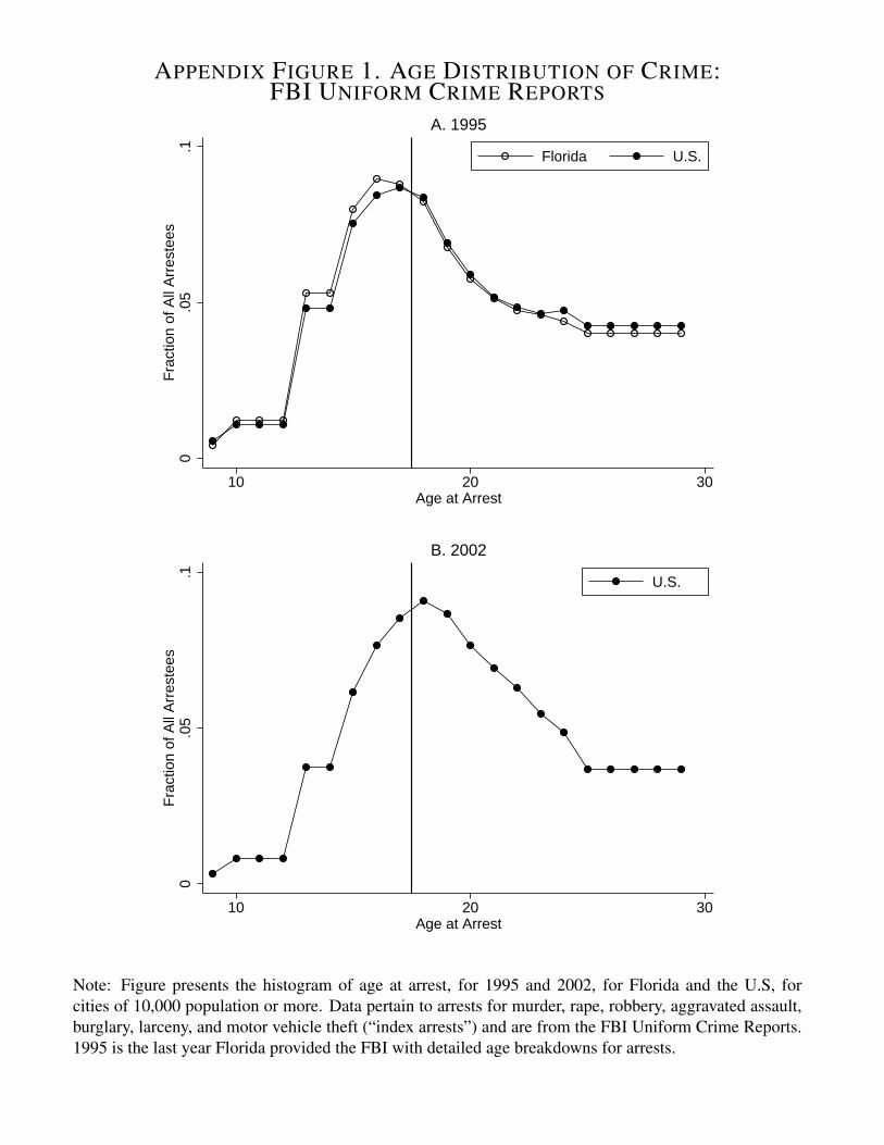
distribution of arrestees at annual frequencies (see Appendix Figure 1).12 In the age range of 17,
12Appendix Figure 1 plots the frequency distribution of age (measured in years), for those arrested for an index
8
18, or 19, for example, youth are graduating from high school, starting new jobs, and develop-
ing physiologically and psychologically in ways that could affect underlying criminal propensities
(Lochner 2004, Wilson and Herrnstein 1985)Since this research design relies heavily on the con-
tinuity of all factors aside from sanctions, in Sections 4 and 5, we assess a number of alternative
ways in which data issues or police discretion in reporting could affect our interpretation of the
discontinuity in arrest rates as a response to more punitive sanctions.
Implementing our research design is straightforward. Here we describe the basic idea behind
the estimation, and later describe minor adjustments to the estimation approach. Suppose we have
a sample of N individuals, and we can track their subsequent offending behavior, starting at age
17. Then for each week, we can calculate the number of individuals arrested for the first time
since 17, as a fraction of those who are still at risk of doing so. If n1, n2, and n3 are the number
of individuals who are arrested in the first, second, and third weeks after their 17th birthday, then
nonparametric estimates of the hazard of arrest are given by h (1) = n1/N , h (2) = n2/ (N − n1),
h (3) = n3/ (N − n1 − n2). We refer to these as local average estimates of the hazard of offense,
and the question is whether the hazard drops off precipitously at age 18.
It is convenient to summarize these averages and the corresponding discontinuity with a flexible
parametric form. To do this, we estimate a panel data logit model, as suggested in Efron (1988).
Specifically, we organize the data set into an unbalanced panel, with N observations for the first
period, N − n1 for the second, N − n1 − n2, and so on. We then estimate the logit
P (Yit = 1|Xt, Dt) = F (X ′tα +Dtθ) (1)
where Yit is the indicator for arrest for persion i in period t,Xt ≡ (1, t− t0, (t− t0)2, . . . , (t− t0)q)′,
q is the order of the polynomial, t0 is the week of the 18th birthday, Dt is 1 if t ≥ t0, and is 0 oth-
erwise, and F (z) = exp(z)/(1 + exp(z)).13 Below, we compare the predicted values from the
crimes (murder, rape, robbery, assault, burlgary, larceny, and motor vehicle theft), as computed using the FederalBureau of Investigation’s Uniform Crime Reports (UCR). Because our administrative data pertain to Florida duringthe period 1995-2002, we show the data for Florida and the U.S. for 1995 and for the U.S. in 2002.
13The vector Xt can also include interactions of the polynomial with the indicator for adulthood. Practically,because the regressors only vary at the level of the group, we estimate the model at the group level and avoid the
9
logit model to the local average hazard estimates h(t), and report a likelihood ratio test for the
restrictions imposed by the logit form.14 As will be clear from the empirical results below, these
models do a good job of providing a parsimonious but accurate fit to the functional form suggested
by the local averages. The reduced-form parameter of interest is θ, the discontinuous change in the
log-odds of committing an offense when the youth turns 18 and immediately becomes subject to
the adult criminal courts.
In a later section, we are also interested in evidence on the incapacitation effect of adult sanc-
tions. For this, we focus on the timing of the second arrest since the 17th birthday, viewed as a
function of age at first arrest since 17. Specifically, we compare how quickly a re-arrest occurs after
being arrested just before age 18, to how quickly it occurs if arrested just after 18. If the marginal
adult takes longer to re-offend, this provides some indirect evidence of an incapacitation effect at
work. While this is not the main target of our analysis, it nevertheless provides some information
on the incapacitation mechanism. This is particularly useful for quantifying the sentence length
elasticity and for calibrating the economic model that we develop below. The implementation of
this analysis follows a more standard regression discontinuity design, where the forcing variable
is the age at first arrest since 17, the “treatment” is whether that arrest occurred before or after age
18, and the dependent variable is whether the second arrest occurs within, for example, 30 days.
4 Data and Sample
In this Section we describe our data, our main analysis sample, and how various features of our
data affect our estimation. We also discuss why our sample is unlikely to be affected by differential
reporting at age 18. For ease of exposition, we defer to Section 5 a more detailed discussion of
expungement of juvenile records.
construction of the (large) micro data set.14That is, we can estimate a logit model with functional form F (W ′tπ), where Wt is a series of indicators for each
week.
10
4.1 Main Analysis Sample
Our analysis uses an administrative database maintained by the Florida Department of Law En-
forcement (FDLE). Essentially, the data consist of all recorded felony arrests in the state of Florida
from 1989 to 2002. The database includes exact date of birth, gender, and race for each person. For
each arrest incident, there is information on the date of the offense, the date of arrest, the county
of arrest, the type of offense, whether or not the individual was formally charged for the incident,
and whether or not the incident led to a conviction and prison term. Importantly, the data are lon-
gitudinal: each arrest incident is linked to a person-level identifier.15 The raw data, therefore, can
be described as a database of individuals, each with an associated arrest history.
From this database, we focus on three key arrest events that define our sample and outcomes of
interest: (1) the first arrest recorded in our administrative data, which we refer to as the “baseline
arrest”, (2) the first arrest since the 17th birthday (we call this the “first arrest”), and (3) the sec-
ond arrest since the 17th birthday (we call this the “second arrest”). Our main analysis sample is
defined by those whose baseline arrest occurs prior to the 17th birthday, for a total of N = 64, 073
individuals.16 To examine deterrence we examine the incidence of the “first arrest” at age 18, and
to provide some evidence on incapacitation, we examine the time between the “first arrest” and
“second arrest” as a function of the age at “first arrest”.
More specifically, for our analysis on deterrrence, we implement the estimation approach de-
scribed in Section 3, with the following modifications and considerations:
• Our last date of observation is December 31, 2002, leading to some individuals being cen-
sored. The standard way to adjust for this is to compute hazards as h(1) = n1/N , h(2) =
n2/ (N − n1 −m1), h(3) = n3/ (N − n1 − n2 −m1 −m2), and so on, where m1 and m2 are
the numbers of individuals who are 1 week and 2 weeks into their 17th year on December 31,
2002 (i.e. censored), respectively. Following Efron (1988), we construct the unbalanced panel
for the logit in an analogous way.
15A more detailed description of the database and its construction is provided in the Data Appendix.16The baseline arrest is allowed to be any arrest. The first and second arrests since 17 are restricted to be index
arrests unless otherwise specified.11
• We note that N = 64, 703 is larger than the true “at risk” population, since at any age a > 17, an
individual could still be incarcerated for the “baseline arrest” or could be incarcerated because of
a non-Index crime arrest that occurred between age 17 and a.17 This fact by itself will not gen-
erate a discontinuity in our estimated hazards, as long as the true “at risk” population is evolving
smoothly in age, particularly at age 18. There is an institutional reason for a discontinuity in the
number “at risk” at age 21; Florida law mandates that no individuals above age 21 can be held in
a juvenile correctional facility. However, there does not appear to be such a reason for an effect
at age 18.
• In terms of the estimated magnitude of our discontinuity, this means our logit estimate θ is ap-
proximately equal to ln(
ρh1−ρh
)− ln
(ρhJ
1−ρhJ
)= ln (h) − ln (hJ) + ln (1− ρhJ) − ln (1− ρh),
where h and hJ are the arrest hazards for an 18.02- and 17.98-year-old, respectively, and ρ ∈
(0, 1) reflects the over-estimation of the risk set. Thus if hJ > h, then ln(
hA1−hA
)− ln
(hJ
1−hJ
)≤
θ < ln (hA) − ln (hJ) < 0. In practice, there is little difference between the upper and lower
bounds.
• Our main analysis sample will include individuals who will more likely be affected by the in-
crease in sanctions. In particular, it seems likely that for this group, there is a positive net benefit
to criminal activity. After all, an individual in our sample has already been arrested at least
once by 17, suggesting that at least one crime was worthwhile to the juvenile. By contrast,
those who have not been arrested as of 17 could potentially include many youth who have vir-
tually no chance of committing a serious crime. For these near-certain law-abiders, it would be
mechanically impossible for their criminal activity to decline after 18.
• It is plausible that those who have already been arrested by age 17 are more likely to under-
stand that there is a difference between the juvenile and adult criminal justice systems; they may
even have been warned about this fact upon their “baseline arrest”. Glassner, Ksander, Berg and
Johnson (1983) provide anecdotal evidence to support this viewpoint.18
17Also, in our main analysis we focus on the incidence of Index felonies, and so at any post-17 age, the individualcould be incarcerated from a non-Index felony arrest.
18For example, responding to a question regarding how he knew that sanctions were more punitive after the ageof criminal majority, one twelve-year-old interviewed by the authors who was earlier arrested for stealing from cars
12
• Our main analysis sample is not likely to be affected by expungement or sealing of criminal
records. In Florida, as in most states, it is possible to have criminal records sealed or expunged.
If juvenile records were systematically missing relative to adult records, then we would be bi-
ased against finding a deterrence effect. But our sample, which requires having at least one
juvenile record, necessarily consists of those who have not expunged their entire juvenile arrest
record. We discuss this in greater detail in Section 5.
Table 1 reports some summary statistics for our main analysis sample. We begin with 64,073
individuals whose baseline arrest occurred prior to 17. As is common in criminal justice data sets,
80 to 90 percent of these arrestees are male, and roughly 50 percent are non-white. The first two
columns present information on the baseline arrest and the first arrest since 17. Age at the baseline
arrest is about 15, and the most common category of offense is property crime, followed by violent
crime. Individuals are distributed evenly among small, medium, and large counties.19 Slightly less
than half of our main analysis sample is observed reoffending after age 17. The sex and gender
composition of arrestees is similar at baseline arrest and first arrest since 17, as is the county-size
distribution. Offenses are distributed somewhat more evenly among the four crime types described
at first arrest since 17 than at baseline arrest. For comparison, the final column reports the same
statistics for all arrests where the individual was 17 or 18 years old at the time of arrest. From the
means, it is apparent that our main estimation sample is broadly representative of this larger arrest
population.
4.2 Measurement and Reporting Discontinuities
Our approach requires that criminality be measured in a smooth fashion near 18. There are some
potential threats to continuous measurement, which we now discuss. One issue is that crimes
are not necessarily defined similarly for juveniles and adults (e.g., truancy, corruption of a minor,
statutory rape, and so on).. To avoid problems with definitions, we consider only crimes that are
responded that the police had told him so: “Police come in our school and a lot of stuff, and I get caught and they tell[sic] me that” (p. 220).
19We classified counties according to total arrests in the FDLE data. Medium counties are Franklin, Palm Beach,Duval, Pinellas, Polk, Escambia, and Volusia. Large counties are Miami-Dade, Broward, and Orange. Remainingcounties are classified as small.
13
well-defined for both juveniles and adults, such as burglary.
Even for crimes that are defined the same way for juveniles and adults, it is still possible that
police officers could exercise discretion in executing an arrest that would lead to discontinuous
measurement. For example, a police officer might view possession of small amounts of marijuana
as forgivable for youth and might overlook the incident upon learning that the individual was still a
minor. This would result in a discontinuous increase at 18 in the probability of observing criminal-
ity in arrest records.20 Alternatively, one could imagine that the officer would view possession of
marijuana as forgivable, but would want to “teach a lesson” to the offender, as long as the cost of
the lesson were not too great. This would result in a discontinuous decrease at 18 in the probability
of observing criminality.
To avoid such problems with discontinuous measurement of criminality at 18, we focus on ar-
rests for so-called Index crimes: murder, rape, robbery, assault, burglary, and theft, including motor
vehicle theft. We are confident that these felonies are sufficiently serious that an arresting officer
would not overlook an offense. An additional benefit of focusing on Index crimes is that these are
the crimes most commonly studied in the literature.
Finally, even if police officers themselves do not exercise discretion regarding making an arrest,
administrative records may be more complete for adult arrests than juvenile arrests. The data from
Florida do not suffer from this problem for the post-1994 period, due to an important criminal jus-
tice reform, the 1994 Juvenile Justice Reform Act, which requires that police departments forward
records of serious juvenile felony arrests to the FDLE (see Section 5.1.2).
5 Evidence on Deterrence and Incapacitation
This section presents our main empirical results. We address two issues. First, we quantify the
deterrence effect of adult criminal sanctions, relative to juvenile criminal sanctions, by studying
the pattern of offending around the 18th birthday. Second, we quantify the incapacitation effect of
adult criminal sanctions, relative to juvenile criminal sanctions, by studying the change around the
20Another example that leads to the same prediction of an increase at 18 in the probability of observing criminalityis from Levitt (1998): there, a hypothetical officer desires to see an arrestee punished and deems that the punishmentaccorded a juvenile is not worth the paperwork required to complete the arrest.
14
18th birthday in durations between arrests.
5.1 Evidence on Deterrence
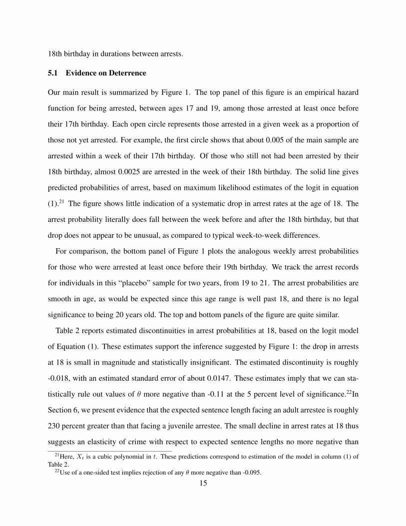
Our main result is summarized by Figure 1. The top panel of this figure is an empirical hazard
function for being arrested, between ages 17 and 19, among those arrested at least once before
their 17th birthday. Each open circle represents those arrested in a given week as a proportion of
those not yet arrested. For example, the first circle shows that about 0.005 of the main sample are
arrested within a week of their 17th birthday. Of those who still not had been arrested by their
18th birthday, almost 0.0025 are arrested in the week of their 18th birthday. The solid line gives
predicted probabilities of arrest, based on maximum likelihood estimates of the logit in equation
(1).21 The figure shows little indication of a systematic drop in arrest rates at the age of 18. The
arrest probability literally does fall between the week before and after the 18th birthday, but that
drop does not appear to be unusual, as compared to typical week-to-week differences.
For comparison, the bottom panel of Figure 1 plots the analogous weekly arrest probabilities
for those who were arrested at least once before their 19th birthday. We track the arrest records
for individuals in this “placebo” sample for two years, from 19 to 21. The arrest probabilities are
smooth in age, as would be expected since this age range is well past 18, and there is no legal
significance to being 20 years old. The top and bottom panels of the figure are quite similar.
Table 2 reports estimated discontinuities in arrest probabilities at 18, based on the logit model
of Equation (1). These estimates support the inference suggested by Figure 1: the drop in arrests
at 18 is small in magnitude and statistically insignificant. The estimated discontinuity is roughly
-0.018, with an estimated standard error of about 0.0147. These estimates imply that we can sta-
tistically rule out values of θ more negative than -0.11 at the 5 percent level of significance.22In
Section 6, we present evidence that the expected sentence length facing an adult arrestee is roughly
230 percent greater than that facing a juvenile arrestee. The small decline in arrest rates at 18 thus
suggests an elasticity of crime with respect to expected sentence lengths no more negative than
21Here, Xt is a cubic polynomial in t. These predictions correspond to estimation of the model in column (1) ofTable 2.
22Use of a one-sided test implies rejection of any θ more negative than -0.095.
15
-0.048. In Section 6, we compare these magnitudes to the predictions from a dynamic economic
model of criminal behavior.
The estimated discontinuity is robust to changes in specification, corroborating the smoothness
assumptions required for our approach. Moving from left to right in Table 2, we control for an
increasing number of factors. Column (1) gives our most parsimonious model, controlling only
for a juvenile/adult dummy and a cubic polynomial in age at current arrest; column (8) gives our
most complex model, adding controls for race, size of county in which the baseline arrest occurred,
offense type of baseline arrest, and a quintic polynomial in age at baseline arrest. In each column,
the added controls are good predictors of the probability of arrest, but in no case does including
additional controls significantly affect the estimated discontinuity.
Appendix Table 3 explores the sensitivity of the estimates to functional form. It reports the
estimated θ for different orders of the polynomial, ranging from a linear to a quintic polynomial
in time and allowing for interactions of the polynomial with the juvenile/adult dummy. The mod-
els are also tested against an unrestricted specification, where the polynomial and the dummy are
replaced with a full set of week-dummies. Overall, the linear and quadratic specifications are ap-
parently too restrictive, and can be statistically rejected by a test against the unrestricted model.
For richer specifications, including ones that include a linear term interacted with juvenile/adult
status, the point estimates range from -0.065 to 0.029, with none of the estimates being statistically
significant. A similar pattern is found when baseline covariates are included.
Below we consider some important potential threats to the validity of our interpretation of these
discontinuities as reflecting deterrence effects.
5.1.1 Transfers of Juveniles to the Adult Criminal Court
The first threat to the validity of our interpretation is the possibility of a lack of a discontinuity in
the “treatment”. That is, while all adults are handled by the criminal courts, and most minors are
handled by the juvenile courts, all states allow a juvenile offender to be transferred to the criminal
16
courts to be tried as an adult (Government Accounting Office 1995).23 In principle, prosecutors
could be more likely to request that a juvenile case be transferred to the criminal justice system
when the arrestee is almost 18. In the extreme case, all arrestees aged 17.8 or 17.9 could be
transferred to the adult court, which would result in no discontinuous jump in the punitiveness of
criminal sanctions and no “treatment”.
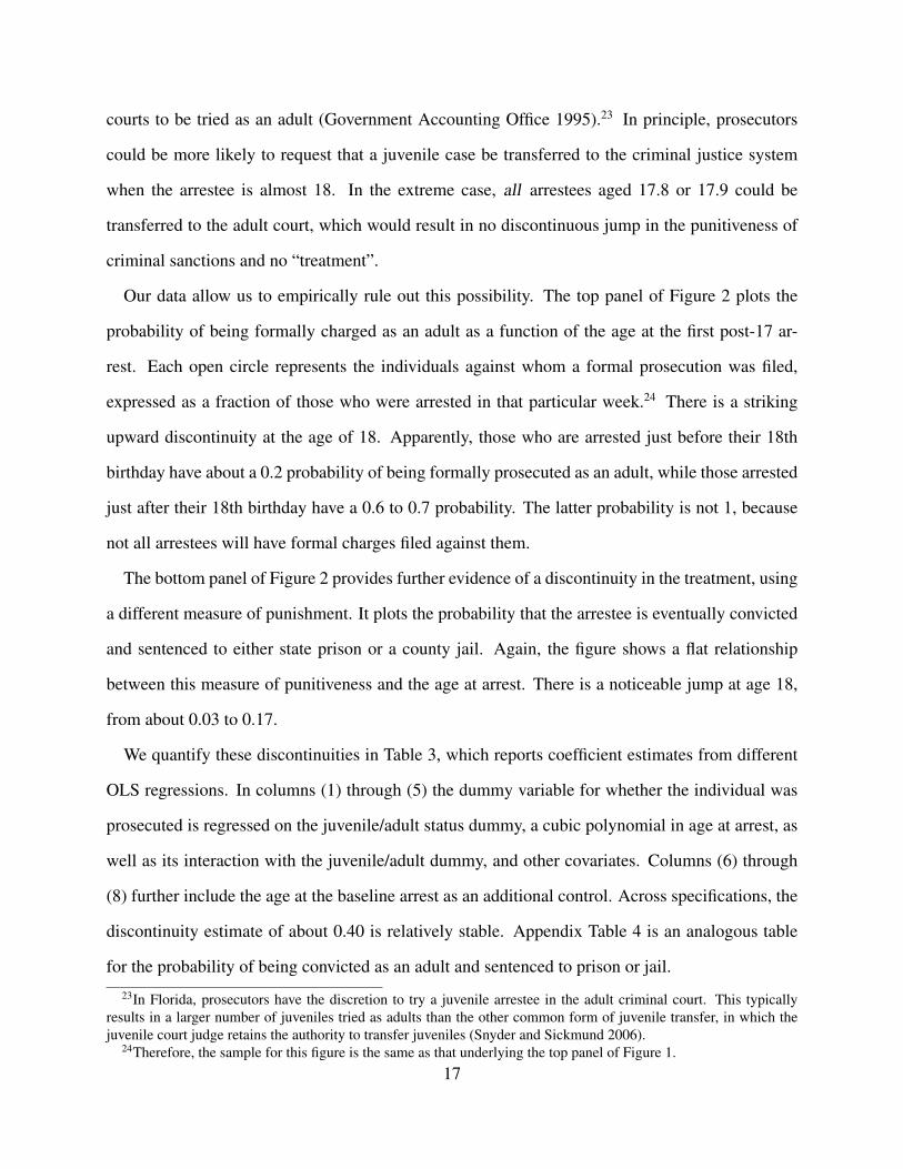
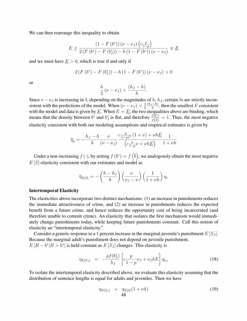
Our data allow us to empirically rule out this possibility. The top panel of Figure 2 plots the
probability of being formally charged as an adult as a function of the age at the first post-17 ar-
rest. Each open circle represents the individuals against whom a formal prosecution was filed,
expressed as a fraction of those who were arrested in that particular week.24 There is a striking
upward discontinuity at the age of 18. Apparently, those who are arrested just before their 18th
birthday have about a 0.2 probability of being formally prosecuted as an adult, while those arrested
just after their 18th birthday have a 0.6 to 0.7 probability. The latter probability is not 1, because
not all arrestees will have formal charges filed against them.
The bottom panel of Figure 2 provides further evidence of a discontinuity in the treatment, using
a different measure of punishment. It plots the probability that the arrestee is eventually convicted
and sentenced to either state prison or a county jail. Again, the figure shows a flat relationship
between this measure of punitiveness and the age at arrest. There is a noticeable jump at age 18,
from about 0.03 to 0.17.
We quantify these discontinuities in Table 3, which reports coefficient estimates from different
OLS regressions. In columns (1) through (5) the dummy variable for whether the individual was
prosecuted is regressed on the juvenile/adult status dummy, a cubic polynomial in age at arrest, as
well as its interaction with the juvenile/adult dummy, and other covariates. Columns (6) through
(8) further include the age at the baseline arrest as an additional control. Across specifications, the
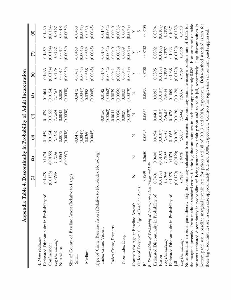
discontinuity estimate of about 0.40 is relatively stable. Appendix Table 4 is an analogous table
for the probability of being convicted as an adult and sentenced to prison or jail.
23In Florida, prosecutors have the discretion to try a juvenile arrestee in the adult criminal court. This typicallyresults in a larger number of juveniles tried as adults than the other common form of juvenile transfer, in which thejuvenile court judge retains the authority to transfer juveniles (Snyder and Sickmund 2006).
24Therefore, the sample for this figure is the same as that underlying the top panel of Figure 1.17
Overall, the evidence strongly suggests that juvenile transfers to the criminal court are not preva-
lent enough to eliminate a sharp discontinuity in the punitiveness of criminal sanctions at 18.
5.1.2 Age-based Law Enforcement Discretion
Another possibility is that offenses committed by juveniles and adults have different likelihoods of
being recorded in our data. For example, it is possible that law enforcement may exercise discre-
tion in formally arresting an individual, based on age. Suppose that the probability of arresting an
individual, conditional on the same offense, is substantially higher for an 18.1 year old than a 17.9
year old. Then it is theoretically possible that the small effects we observe are a combination of a
negative deterrence effect and a positive and offsetting jump in the arrest probability.
There are a number of reasons why we believe this is not occurring in our data. First, our anal-
ysis focuses on very serious crimes, where it seems unlikely that an officer would be willing to
release a suspect without an arrest, purely on the basis of the individual’s age. For example, all
Index crimes involve a victim. We suspect that the pressure to capture a suspect is too great for
officers to be willing to release an individual suspected of committing an index crime. By contrast,
for relatively less serious crimes such as misdemeanors or drug possession, it is more plausible
that officers might exercise discretion in making the arrest.
Second, each individual in our main estimation sample already has a recorded formal arrest as
of age 17, when we begin following their arrest experiences. Thus, it seems unlikely that the law
enforcement agency will exercise leniency in recording an arrest: if a juvenile is apprehended just
before his eighteenth birthday, it is too late to do anything to keep the youth’s felony arrest record
clean.
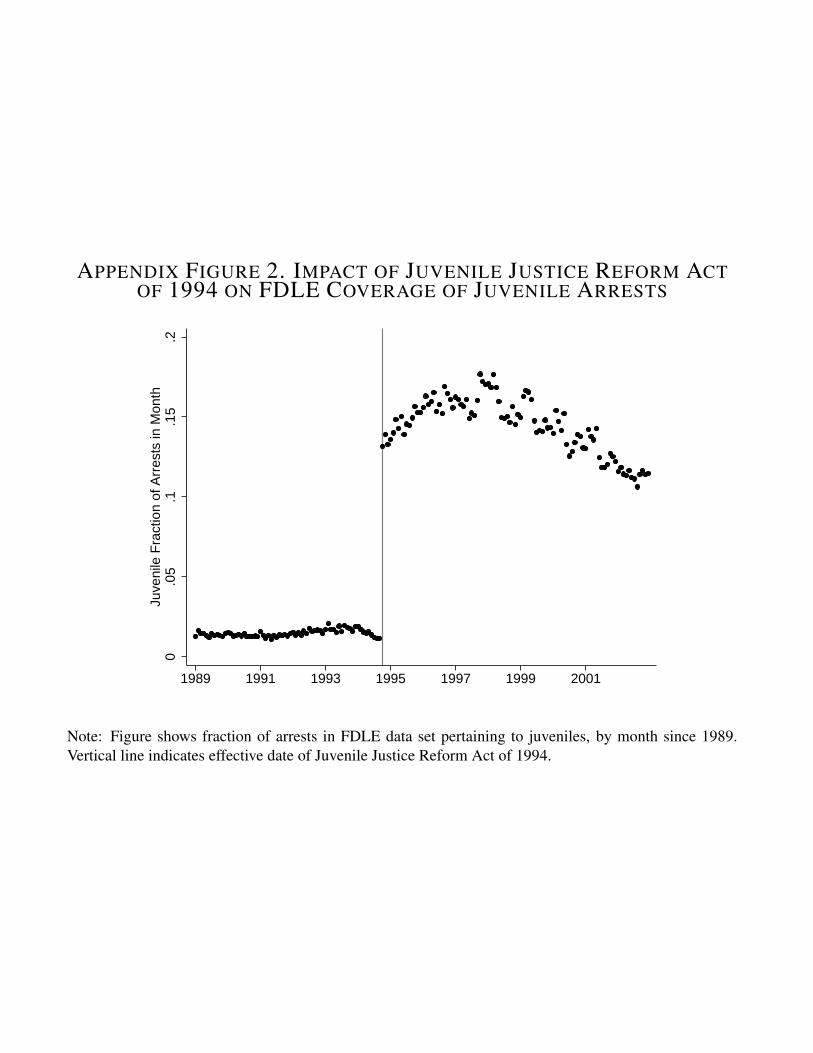
Third, our analysis focuses on arrests since 1994, the year of Florida’s Juvenile Justice Reform
Act (JJRA), which requires that felonies and some misdemeanors committed by juveniles be for-
warded to the state for inclusion in the criminal history records maintained by the FDLE.25 The
25The implication of this Florida law was summarized by a state attorney general opinion in 1995: “UnderFlorida law, crime and police records regarding crime have been a matter of public record. With limited exceptions,however, the identity of a juvenile who committed a crime has been protected. With the enactment of Chapter94-209, Laws of Florida, an omnibus juvenile justice reform measure, the Legislature has amended the confidentialityprovisions relating to juvenile offenders to allow for greater public dissemination of information. The clear goal of
18
impact of this law on the prevalence of juvenile records is shown in Appendix Figure 2. This figure
show the number of juvenile arrests as a proportion of all arrests in the FDLE arrest data, by month
from 1989 to 2002. There is a marked discontinuity in the ratio at October 1994, the month the
JJRA took effect.
Finally, if juvenile and adult arrests had different likelihoods of being recorded in our data, we
would expect to observe significant heterogeneity in the estimated θ, by different groups of in-
dividuals, and different crime types, since it is likely that any off-setting measurement problems
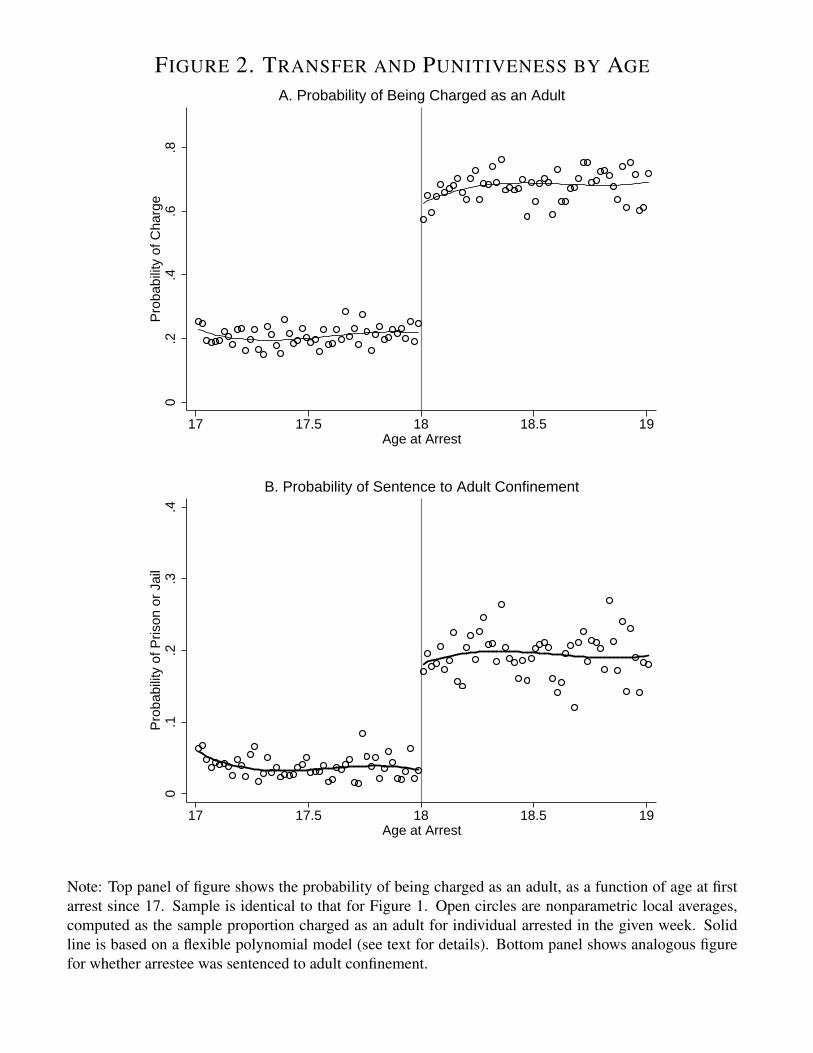
will vary by characteristics of the individual, as well as by crime type. Figure 3 provides evidence
contrary to this prediction. The top panel of the figure disaggregates the arrest probabilities from
the top panel of Figure 1 into two components: property and violent crime. The figure shows that
the estimated discontinuity is essentially the same for the two categories of crime.
We also estimate θ separately by sub-groups defined by key correlates of arrest propensities, and
find no evidence of significant negative effects for some groups being masked by positive effects of
other sub-groups. Table 4 reports estimates from interacting the juvenile/adult dummy with race,
size of county of the baseline arrest, and offense of the baseline arrest. The estimates for these
different sub-groups range from -0.07 to 0.09. These estimates are generally of small magnitude;
moreover, none of the 20 are statistically significant. Finally, we fail to reject the null hypothesis
that the interaction effects are all zero in Table 2, and this holds for all specifications considered.
Although our analysis focuses on index crimes, for completeness we show the results for all
remaining offenses in the bottom panel of Figure 3. We consider the potential for arrest discretion
to be the most serious for these non-index crimes, which include “victimless” offenses such as
drug possession. Here, the cubic polynomial predictions do show a small perverse discontinuity,
although the local averages do not reveal an obviously compelling jump at age eighteen. Still, if
law enforcement discretion is of particular concern, a conservative approach would be to discount
the results for non-index crimes.
the Legislature was to establish the public’s right to obtain information about persons who commit serious offenses,regardless of age” (Butterworth 1995, p. 274).
19
5.1.3 Expungement of Juvenile Records
A third possibility is that the ability of individuals to expunge and seal juvenile arrest records
could generate downward biased estimates of arrest rates for juveniles, and hence mask any true
deterrence effects. Florida law allows individuals who successfully complete a juvenile diversion
program to apply to have all juvenile records expunged (Fla. Stat. 943.0582). Apart from this
provision, Florida law also mandates that juvenile arrest histories be expunged when the individual
turns 24.26
Our choice of sample, however, circumvents these two expungement provisions in the following
ways. First, our estimation sample is restricted to those committing baseline crimes before age 17
but subsequent to January 1, 1995. Therefore, the individuals are not yet 24 by the end of our sam-
ple frame, and thus will not be subject to the time-activated expungement. Second, a requirement
for inclusion in our sample is an observed arrest record prior to age 17. Thus, by construction,
the individuals in our main estimation sample did not have their complete juvenile arrest history
expunged.
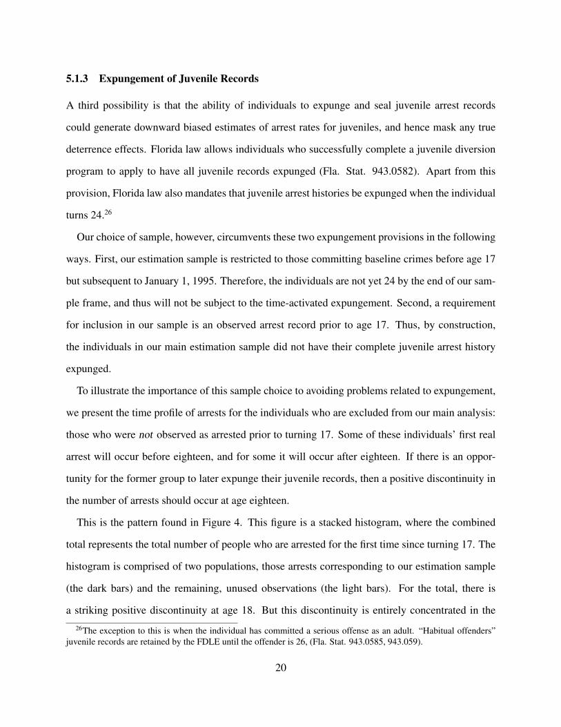
To illustrate the importance of this sample choice to avoiding problems related to expungement,
we present the time profile of arrests for the individuals who are excluded from our main analysis:
those who were not observed as arrested prior to turning 17. Some of these individuals’ first real
arrest will occur before eighteen, and for some it will occur after eighteen. If there is an oppor-
tunity for the former group to later expunge their juvenile records, then a positive discontinuity in
the number of arrests should occur at age eighteen.
This is the pattern found in Figure 4. This figure is a stacked histogram, where the combined
total represents the total number of people who are arrested for the first time since turning 17. The
histogram is comprised of two populations, those arrests corresponding to our estimation sample
(the dark bars) and the remaining, unused observations (the light bars). For the total, there is
a striking positive discontinuity at age 18. But this discontinuity is entirely concentrated in the
26The exception to this is when the individual has committed a serious offense as an adult. “Habitual offenders”juvenile records are retained by the FDLE until the offender is 26, (Fla. Stat. 943.0585, 943.059).
20
unused sample (the upper part of the stacked graph).27
5.2 Evidence on Incapacitation
Up to this point, we have examined the evidence for a deterrence effect of adult criminal sanctions,
relative to juvenile criminal sanctions. We now ask: What is the incapacitation effect of treating
an apprehended offender as an adult instead of a juvenile? To answer this, we use a standard re-
gression discontinuity design, where the “treatment” of adult status is a discontinuous function of
the forcing variable of age at “first arrest”. As described in Lee (2008), if there is imprecise sort-
ing around the age of majority, then being treated as an adult has statistical properties similar to a
randomized experiment.28 Indeed, in the analysis above we are unable to detect strong evidence of
such sorting behavior. In essence, our results on deterrence imply that this design passes the test
of manipulation of the forcing variable suggested in McCrary (2008).
The RD design is illustrated in Figure 5. The top panel of the figure plots the probability that
the “second arrest” occurs within a specific window of time since the “first arrest”, as a function
of the age at “first arrest”. Specifically, the leftmost open circle indicates that among those whose
“first arrest” occurs the week after their 17th birthday, the probability of re-arrest within the subse-
quent 30 days is about 15 percent. Among those whose “first arrest” occurs just before their 18th
birthday, the probability of re-arrest within the subsequent 30 days is about 20 percent.
There is a sharp discontinuity in the probability of re-arrest at age 18, with 18.02 year olds hav-
ing a probability of re-arrest within 30 days of about 10 percent. A natural explanation for this
difference is that being handled by the adult criminal court leads to a longer period of custody than
does being processed as a juvenile. The 17.98 year old is released earlier and hence has a greater
opportunity to re-offend within any short time window, compared to the 18.02 year old.
The solid circles and open triangles plot the same kind of graph, except that we examine the
probability of a re-arrest occurring within 120 and 365 days after the “first arrest”. The probabilities
27The dark bars represent the values used in the upper panel of Figure 1, except that Figure 1 normalizes each valuewith the at-risk population at each point in time to provide a probability value.
28By “imprecise sorting” we mean that for each individual, the density function of age at arrest is continuous at 18.See Lee (2008) for further discussion.
21
are higher for 120 and 365 days, since the probability of re-arrest increases with the window width.
The length of the follow-up period is arbitrary. The bottom panel of Figure 5 plots the profile
of discontinuity estimates using follow-up lengths ranging from 1 to 500 days. For example, the
estimates at 30, 120, and 365 days in the bottom panel, emphasized with large solid triangles,
correspond to the discontinuity estimates from the top panel of the figure. Overall, the bottom
panel shows that already by 20 days, there is a large divergence in the cumulative number of arrests
between those who are arrested as a 17.98 year-old and those arrested at age 18.02, for example.29
This divergence continues to grow, slowing down at around 100 days after the initial arrest.30
6 Predicted Effects from a Dynamic Model of Crime
In this Section we interpret the magnitudes of our estimated deterrence effects through the lens
of an economic model of criminal behavior. We develop a dynamic extension of Becker’s (1968)
model of crime. We first consider how large of a discontinuity we should expect given our model,
which can be calibrated to readily available sample means, and standard assumptions.We then use
our model to draw a precise link between our discontinuity estimates and policy-relevant deter-
rence elasticities of interest. Under some fairly mild assumptions, we calculate the most negative
policy-relevant deterrence elasticities consistent with both our model and our estimates.
6.1 A Dynamic Model of Criminal Behavior
The essence of Becker’s model of crime is that an individual weighs the expected benefits (e.g.
monetary or otherwise) against the expected costs (e.g. fines, disutility from being incarcerated).
This basic notion can be captured in a discrete-time dynamic model, in which the individual faces
a criminal opportunity every period and chooses between committing the offense and abstaining.
29It is worth noting that by Florida law, juvenile pre-trial detention cannot be longer than 21 days. No suchrestriction applies to adult pre-trial detention. Investigation of the juvenile hazard of re-offense indicates a strongspike near 21 days.
30Note also that an incapacitation interpretation is not the only one consistent with the data. Alternatively, thesedata are also consistent with no difference between juvenile and adult lengths of incarceration. This could occurif being incarcerated in the adult criminal justice system had a negative causal effect on criminal propensities uponrelease. This notion is sometimes referred to as “specific deterrence”, particularly in the criminology literature. SeeCook (1980) for discussion of the concept and Hjalmarsson (2009) for a recent empirical approach. This alternativeinterpretation requires a mechanism by which the quality of the experience of being incarcerated as an adult inducesindividuals to be more law-abiding upon release.
22
If he commits the offense, there is a chance that he will be apprehended and incarcerated for a
random number of periods before being released.
The model described below closely resembles a canonical job search model (McCall 1970). The
elements of the model are as follows:
• In each period, a “criminal opportunity” B is drawn from a distribution with cumulative distri-
bution function F (b) and density f (b). Criminal opportunities are assumed to be positive.31
• The individual chooses to offend or abstain. In period t, if he abstains, he receives flow utility
ut = a. If he offends, with probability 1 − p, he obtains the flow utility ut = a + B. With
probability p, he is apprehended and will be incarcerated for the next S periods (inclusive of
the current period t). While incarcerated, he receives flow utility ut, ut+1, . . . , ut+S−1 = a − c,
where c is a positive per-period utility cost of being incarcerated.
• S is a random draw from a distribution given by the probabilities {πs}∞s=1
• The individual chooses to offend or abstain in each period to maximize Et [∑∞τ=t δ
τ−tut], where
Et is the expectation operator conditional on information available as of period t, δ is the dis-
count factor, and ut is one of a − c, a, or a + B, depending on the agent’s choices, whether he
has been apprehended for any crimes committed, and whether he is currently detained.
The Bellman equation for this problem is
V (b) = max
{a+ δE[V (B)], p
∞∑s=1
πs
[(a− c) 1− δs
1− δ+ δsE[V (B)]
]+ (1− p)
[a+ b+ δE[V (B)]
]}(2)
The first argument of the max function is the payoff from abstaining. The second argument is an
expected payoff from committing the offense. If caught and incarcerated for s periods, the payoff is
(a−c) (1 + δ + δ2 + . . .+ δs−1)+δsE [V (B)]. If not apprehended, the payoff is a+b+δE[V (B)].
The individual’s optimal strategy is characterized by a “reservation” threshold, b∗, such that
when B > b∗, he commits the crime, and when B < b∗ he abstains.32 Equating the two arguments31An earlier draft (Lee and McCrary 2005) considered a model in which there was heterogeneity in p, the
probability of apprehension.32This mimics the standard “reservation wage” property of a job search model. See, for example, the textbook
treatments in Adda and Cooper (2003) and Ljungqvist and Sargent (2004).23
of the max function above leads to an expression for the reservation benefit:
b∗ = cp
1− p
[1 +
∞∑s=1
πsδ − δs
1− δ
(1 +
(1− δ)E [V (B)]− ac
)](3)
We make the following observations about this expression:
• When δ = 0, it becomes b∗ = c p1−p , which implies that the crime will be committed whenever
the ratio of the net benefit to net cost, Bc
, exceeds the odds ratio of apprehension, p1−p . This is
precisely the notion put forth in a standard (and static) Becker model of crime. It is intuitive that
when the individual completely discounts the future, the length of incarceration, S, is irrelevant.
• Similarly, b∗ = c p1−p if the punishment is only 1 period long (π2, π3, . . . = 0).
• The second term inside the square braces thus captures the increased expected cost to offending
due to a period of incarceration longer than 1 period. During incarceration, the offender bears
the per-period cost c, but also is not able to exercise the option of committing offenses during
this period. This lost option value is contained in the term (1−δ)E[V (B)]−ac
. The Appendix shows
that the annuitized value of the dynamic program can be expressed as
It is intuitive that the option value, the second term, is the probability of an arrival of a worth-
while crime times the probability of not being apprehended times the expected benefit condi-
tional on it being optimal to commit the offense.
We obtain the following intuitive comparative statics (proof in Appendix). The crime rate, which
is given by 1− F (b∗), decreases with:
• Higher discount factor, δ. As the individual places more weight on future utility, the penalty of
incarceration poses a higher cost.
• Higher per-period direct utility cost to incarceration, c.
• Higher apprehension rates, p.
24
• Longer sentence lengths. Any rightward shift in the distribution of the incarceration length S
(i.e., the new distribution first-order stochastically dominates the old) decreases offending.
6.2 Benchmark Model Calibration and Predicted Values for θ
In this section, we calibrate the above model to produce predictions on the size of the reduced-form
estimates of θ from our logit estimation. This exercise answers the question “In this economic
model of crime, how large of a θ would we have expected to observe?” We have
θ = ln
(Pr18.02 [Arrest]
1− Pr18.02 [Arrest]
)− ln
(Pr17.98 [Arrest]
1− Pr18.98 [Arrest]
)(5)
= ln
(1− (1− p (1− F (b∗)))7
(1− p (1− F (b∗)))7
)− ln
(1− (1− p (1− F (b∗J)))
7
(1− p (1− F (b∗J)))7
)
where Pr17.98 [Arrest], for example, is the probability of a juvenile being arrested one week prior to
his 18th birthday. In the calibration of our model, we take each period to be a single day. The daily
probability of arrest for an adult is p (1− F (b∗)). For a 17.98-year-old, it is p (1− F (b∗J)), where
b∗J is the juvenile reservation benefit, defined below. For our calibration exercise, we let a = 0 and
c = 1 , two normalizations that are innocuous as long as we interpret the benefit B as the ratio of
the net benefit to the per-period cost of being incarcerated.33
Combining Equations (3) and (4) yields an implicit equation for b∗, and a similar approach
delivers an implicit equation for b∗J :
b∗ =p
1− p
[1 +
∞∑s=1
πsδ − δs
1− δ{1 + (1− F (b∗))(1− p)E[B − b∗|B > b∗]}
](6)
b∗J =p
1− p
[1 +
∞∑s=1
πJsδ − δs
1− δ{1 + (1− F (b∗))(1− p)E[B − b∗|B > b∗]}
](7)
The only difference in these two expressions is the distribution of sentence lengths.
In our benchmark calibration, we (1) let S and SJ be distributed as a discretized exponential,
withE [S] = 207 (days) andE [SJ ] = 63, (2) let p = 0.08 and δ = .95(1/365), and (3) letB be expo-
33Maximizing Et [∑∞τ=t δ
τ−tut] is equivalent to maximizing Et[∑∞
τ=t δτ−t (ut−a
c
)]. Thus, no matter the values
of a and c, the solution will be equivalent to considering a problem where the flow utility takes the values of −1, 0,or Bc .
25
nentially distributed with parameter λ = 4.56. With these magnitudes and parameterization, Equa-
tions (6) and (7) are used to solve for b∗ and b∗J , which yields daily arrest hazards p (1− F (b∗))
and p (1− F (b∗J)), which are then used to produce a predicted θ using Equation (5).34
The magnitudes we use for these parameters have some empirical backing:
• Our model suggests that we can use the evidence from Figure 5 to estimate the gap E [S] −
E [SJ ]. Specifically, we compute the time between “first arrest” and “second arrest” for 17.98-
and 18.02-year olds. According to our model, that difference is an estimate of E [S]−E [SJ ].35
Using the same data and similar approach as the RD analysis in Figure 5, we estimate a Weibull
duration model, where the duration is a function of a cubic in age and a dummy variable for
adulthood.36 This yields estimated durations of approximately 962 and 818, for adults and juve-
niles, respectively, and a gap of E [S]− E [SJ ] = 144 days.
• We obtain E [SJ ] = 9.05 × 7 ≈ 63 from Appendix Table 1, which reports average incar-
ceration lengths from a completely different data source (see Data Appendix for discussion).
This approach suggests E [S] = 63 + 144 = 207. We note that this different data source yields
E [S] = 46.48×7 ≈ 325 days, which implies a differenceE [S]−E [SJ ] of 262; we take a more
conservative view of the power of our research design by choosing the smaller gap of 144 days.
• Appendix Table 2 provides estimates of clearance rates and reporting rates for Index crimes in
2002. These numbers suggest p = 0.08.37
• Finally, we choose the λ such that the implied b∗, via Equation (6), is consistent with our esti-
mate of the adult arrest hazard p (1− F (b∗)) of 0.0013, which is computed as follows. Using
34As noted in Subsection 4.1, ln(
h1−h
)− ln
(hJ
1−hJ
)≤ θ < ln (h) − ln (hJ) < 0, where h and hJ are the true
arrest hazarads for the marginal adult and juvenile. In our calibrations, we report the smaller (in magnitude) of thetwo, ln (hA)− ln (hJ), but in practice, there is very little difference between the bounds.
35According to our model, the average duration between arrests as an adult is E [S] + 1p(1−F (b∗)) ; that is, once an
adult is arrested, the time until the next arrest is given by the period of incarceration S plus the time between being re-leased and the next arrest, which is exponentially distributed with hazard p (1− F (b∗)) (and hence mean 1
p(1−F (b∗)) ).Similarly, the time until next arrest for a juvenile arrested just before his 18th birthday is given byE [SJ ]+ 1
p(1−F (b∗)) .36Specifically, we model the juvenile and adult durations as separate Weibull models, allowing both the shape and
scale parameters to depend on a cubic in age at initial arrest.37Clearance rates are the fraction of offenses known to police for which an individual has been arrested and handed
over to prosecutors. These rates are estimated using the UCR data. Reporting rates are the fraction of index offensesreported to police and are based on the NCVS. The aggregate clearance rate is 20 percent, and the aggregate reportingrate is 42 percent, for an approximate 0.2× 0.42 = 0.08 probability of apprehension.
26
the same Weibull estimates from above, we have 1p(1−F (b∗))
= 962− E [S] = 962− 207 = 755.
The implied daily arrest hazard is p (1− F (b∗)) = 1755
, or about 0.0013.
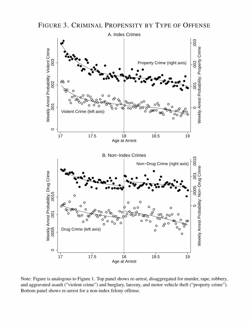
The results of these calculations are presented in the first row of Table 5, which shows that this
set of parameters would predict a discontinuity estimate of -2.76. As noted above, our standard
errors are small enough to statistically rule out values of θ more negative than about -0.11. Thus,
in the context of the model outlined, a benchmark calibration suggests that the data are at odds
with long time horizons. The rest of Table 5 reports our exploration of the sensitivity of the pre-
dicted θ to different parameter values for the model. We vary each parameter one at a time, while
maintaining the values for the other parameters in the benchmark calibration in the top row.
While the predicted θ increases in magnitude with increasing p, from -2 to -3.74 as p ranges
from 0.025 to 0.400, none of the predicted θs are close to our point estimate of -0.018. Indeed,
none are close to the outer edge of our confidence region for θ, -0.11. Note that the extreme values
of p that we consider, 0.025 and 0.400, are at odds with the evidence summarized in Appendix
Table 2. The conclusion that our estimates are much smaller than the benchmark prediction seems
robust to assumptions regarding p.
We next consider the distribution of sentence lengths. Our benchmark calibration assumes sen-
tences are distributed as a discretized exponential. The exponential distribution is a special case
of the Weibull distribution, with the shape parameter of the Weibull equal to 1. To explore the
sensitivity of the predicted θ to the assumed shape of the distribution, we vary the shape parame-
ter for the juvenile and adult sentence length distribution over 0.25, 0.40, 2.0, and 4.0. For each
such shape parameter, kJ and kA, we adjust the Weibull scale parameters to match the means
E [SJ ] = 63 and E [S] = 207. To gain intuition about these changes, note that when the shape
parameter is 0.25, the density is more convex and skewed, while when the shape parameter is 4,
the shape of the distribution is more akin to that of the chi-square distribution. The table shows that
the shape of the sentence length distribution affects our predictions only negligibly. For example,
with the shape parameter for the juvenile distribution, kJ , equal to 0.25, the predicted θ is -2.95
and with a shape parameter of 4.0, the predicted θ is -2.76. Results for the impact of the adult27
shape parameter, kA, are similar.38
The effect of different discount factors is shown in the last row of Table 5. When the discount
factor declines from 0.95 to 0.01 on an annual basis, the magnitude of the predicted θ falls from
-2.50 to -1.57. This is a notable pattern, because – unlike the case of p or E [S] and E [SJ ] – we
have no independent information on the discount factor. The relevant discount factor is that for
the marginal offender, and could be much smaller than 0.95. We note that in some settings, such
as the market for subprime loans, the literature has documented behaviors that are consistent with
extremely small discount factors (Adams, Einav and Levin 2009).39 Most importantly, discount
factors could be much smaller when arrestees are drug-users, a common pattern. For example,
there is evidence from urinanalysis that a large fraction of arrestees test positive for drug use. In
2000, 61.8 percent of Fort Lauderdale and 62.8 percent of Miami arrestees tested positive for at
one or more of the following: cocaine, marijuana, opiates, methamphetamine, or PCP (National
Institute of Justice 2003). This suggests the prevalence of short time horizons and low discount
factors among the relevant subpopulation. In our model, when the discount factor is arbitrarily
small, the predicted θ is arbitrarily close to zero.
Finally, we consider the impact of changes in the shape of the criminal benefit distribution, the
other element of the model for which we have no independent information. In the benchmark cal-
ibration, this distribution was assumed to be exponential. Generalizing to a Weibull distribution,
we vary the shape parameter, k, over 0.25, 0.40, 2.0, and 4.0. When k = 4.0, many individuals are
on the margin of the crime participation decision, but when k = 0.25, few individuals are on the
margin. We see that as the shape parameter falls from 4.0 to 0.25, the predicted θ falls in magnitude
from -3.84 to -1.03.
We conclude from this analysis that a reasonable benchmark parametric model with standard
“patient” discount factors predicts much larger discontinuities in offending at age 18 than we ob-
38This robustness to distributional assumptions on the sentencing side is due to the fact that the distribution ofsentences only matters to the extent that it affects the expectation of δ−δS
1−δ , which is nearly unchanged by changes tothe shape of the underlying distribution, assuming that sentences are somewhat long.
39Similarly, in states without interest rate regulations, pawnbrokers charge interest rates implying annual discountfactors of 0.3 (Caskey 1996).
28
serve in our data. Given that the predictions seem somewhat sensitive to the discount factor and the
shape of the benefit distribution, when we consider the policy implications of our estimates below,
we relax the parametric assumptions on the benefit distribution, and present a bounding analysis.
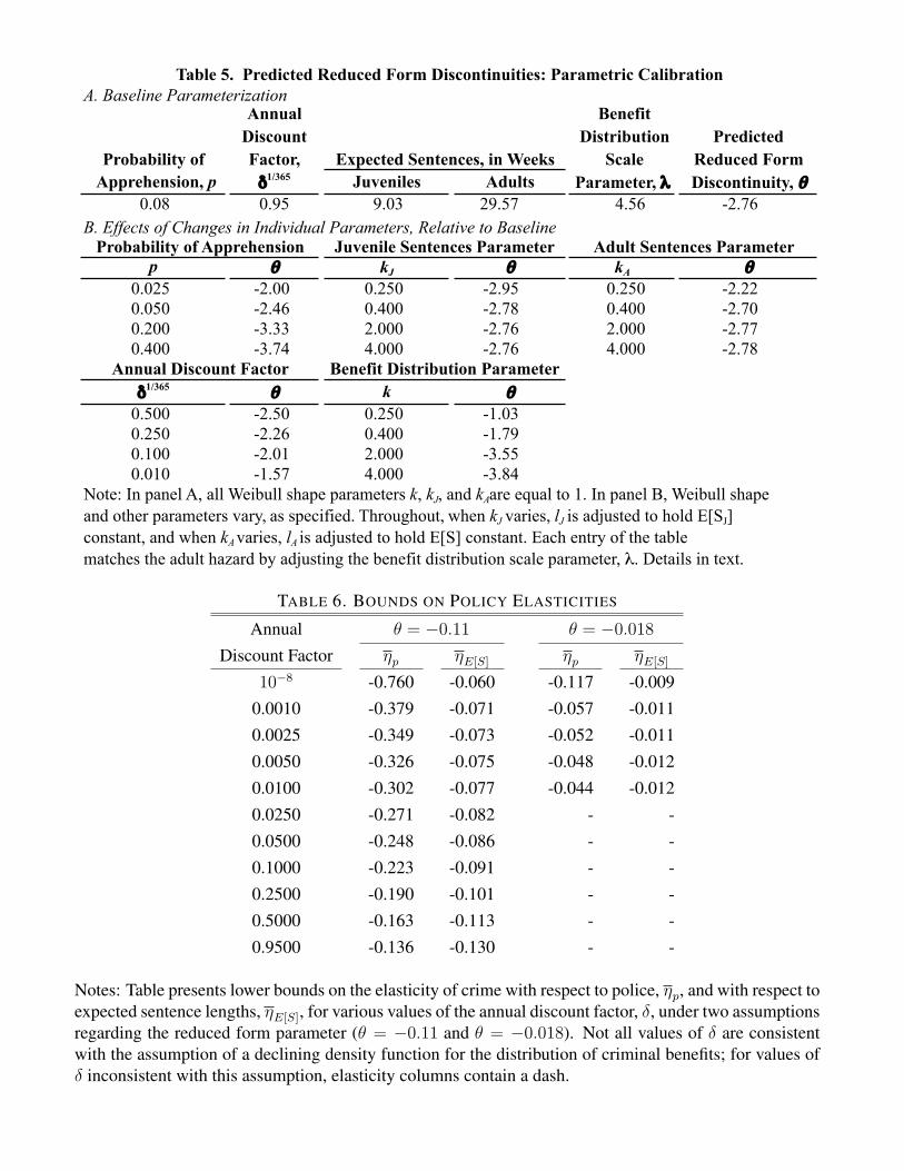
6.3 Policy Implications
We use our model to consider the decline in crime associated with two key criminal justice policy
reforms: increases in the expected sentence length facing offenders, and increases in the probabil-
ity of apprehension. In elasticity terms, the responsiveness of the crime rate to these policy reforms
can be derived as
ηE[S] ≡ ∂(1−F (b∗))∂E[S]
E[S]1−F (b∗)
= −pf(b∗)h
E [S] ∂b∗
∂E[S]= −
[(hJ−hh
)/(ν−νJν
)]ην(
11+νh
)f(b∗)
f(b)
ηp ≡ ∂(1−F (b∗))∂p
p1−F (b∗)
= −pf(b∗)h
p∂b∗
∂p= −
[(hJ−hh
)/(ν−νJν
)]κ(
11+νh
)f(b∗)
f(b)
where h = p (1− F (b∗)), hJ = p (1− F (b∗J)), ν =∑∞s=1 πs
δ−δs1−δ , νJ =
∑∞s=1 π
Jsδ−δs1−δ , ην ≡
∂ν∂E[S]
E[S]ν
, κ ≡c p
(1−p)2(1+ν)+νhE[B−b∗|B>b∗]
c p1−pν+νhE[B−b∗|B>b∗] , and b ∈ (b∗J , b
∗) is such that f(b)
=F (b∗)−F(b∗J)
b∗−b∗J(see
Appendix for detailed derivation).
Since θ ≈ −hJ−hh
, these formulas show that our discontinuity estimate is proportional to the
policy relevant elasticities ηE[S] and ηp. The second component of these formulas, ν−νJν
, gives the
percent increase in the expected discounted number of periods of incarceration when crossing the
age 18 threshold. This term reflects the influence of δ as well as the distributions of S and SJ . For
patient individuals, ν−νJν
is approximately equal to E[S]−E[SJ ]E[S]
.
The third components are unique to each elasticity. In the case of ηE[S], ην reflects the percentage
change in ν brought on by a percentage change in the expected number of periods of incarceration.
In the case of ηp, κ is a quantity that reflects the percentage change in p that has the equivalent
impact as a percentage change in ν.
The fourth term 11+νh
is an offsetting adjustment that accounts for the following effect: when the
expected costs of offending rise, the option value of being free is reduced, which in turn dampens
29
the per-period cost of incarceration.40 Finally, the fifth term f(b∗)
f(b)reflects the shape of the benefit
distribution: f(b∗)
f(b)= 1 if the density of B is flat between b∗J and b∗, but more generally this ratio
may differ from 1.
We can calibrate our benchmark model to ask what policy elasticites our estimates imply. For
example, we can adjust the discount factor so that the predicted θ matches -0.11, the outer edge of
our confidence interval. This yields a daily discount factor of 0.71, which predicts elasticities of
ηE[S] = −0.049 and ηp = −4.44. We could have alternatively kept δ fixed and attempted to match
the predicted θ to the observed θ by adjusting the shape parameter k of the benefit distribution.
Since it is arbitrary which parameter to adjust, in the next Subsection, we consider a wide range of
δ, while relaxing the parametric restriction on the benefit distribution.
6.4 Nonparametric Bounds on Policy Elasticities
We now explore the range of policy elasticities that are consistent with our discontinuity estimates,
relaxing the parametric restriction on the shape of the criminal benefit distribution.
We first note that it is always possible to construct a distribution forB that is both consistent with
any negative value of θ, yet yields policy elasticities of zero or −∞. One needs to simply set the
density f (b∗) to zero or arbitrarily large. This fact is not unique to our dynamic model: this will be
the case with any model that has a distribution of criminal activity and a minimum-cost threshold.
It is thus more informative and plausible to consider some mild restrictions on the benefit distri-
bution. We focus on the assumption that the density of benefits is weakly declining in B. This as-
sumption has some economic justification, going back at least to Stigler (1970) and Viscusi (1986).
Intuitively, as these authors have argued, by the nature of crime, opportunities that are valuable to
the offender are costly for the victim. This provides incentives for victims to take greater precau-
tion regarding more valuable criminal opportunities (e.g., deadbolt locks, car alarms, and mace).
It is thus plausible to assume that more valuable opportunities are scarce, relative to less valuable
opportunities.
We show in the Appendix that the assumption of a declining density of B delivers an upper
40See Appendix for discussion.
30
bound on the magnitude of the policy elasticities ηE[S] and ηp. In particular, we show that
ηE[S] > ηE[S] ≡ −[(hJ − hh
)/(ν − νJν
)]ην
(1
1 + νh
)
ηp > ηp ≡ −[(hJ − hh
)/(ν − νJν
)]κ(
1
1 + νh
)
where ην ≡ ∂ν∂E[S]
E[S]ν
, and κ ≡c p
(1−p)2(1+ν)+νhE
(c p1−pν+νhE)
.41 Both ηE[S] and ηp can be computed using infor-
mation on discount factors, the distribution of sentence lengths, and our empirical findings on arrest
rates for youthful offenders at age 17.98 and 18.02. Other than assuming a declining density, no fur-
ther information regarding the distribution of criminal benefits is required to obtain these bounds.
Table 6 reports our estimates of the elasticity bounds ηp and ηE[S] for our point estimate of
θ = −0.018 and for the edge of our 95 percent confidence interval, θ = −0.11, using various
values of the discount factor. Using the most negative value of θ = −0.11, the sentencing elastic-
ity ranges from -0.130 to -0.060, and the probability of apprehension elasticity ranges from very
large negative values to -0.136. If we use our point estimate, the sentencing elasticity ηE[S] varies
only slightly, from -0.013 to -0.010, while the probability of apprehension elasticity ηp varies from
-0.117 to -0.044.
Interestingly, for the case of θ = −0.018, there are some δs that cannot be rationalized within
the framework of the model. That is, as we show in the Appendix, we find that if θ = −0.018,
then there exists no E [B − b∗|B > b∗] that is consistent with both the model and the restriction of
a weakly declining density.
Overall, the table points to two policy conclusions. First, if one believes that the probability of
apprehension elasticity is large, then this implies very low discount factors, and consequently very
low sentence length elasticities. Second, across the entire range of permissable discount factors,
all of the sentence length elasticities are generally small in magnitude.
41E is a (strictly positive) lower bound for E [B − b∗|B > b∗] which we derive in the Theory Appendix under theassumption of a declining density.
31
7 Conclusion
Over the past 40 years, the incarceration rate in the United States has soared, from 161 persons
in prisons or jails per 100,000 in 1972 to 761 persons per 100,000 in 2006. Indeed, despite the
declining crime rates of recent years, prison and jail populations continue to climb, as the full
impact of sentencing reforms from previous years becomes felt (Raphael and Stoll 2009).42 For
economists, it is natural to wonder if more severe prison sentences deter crime by a sufficient
amount to make paying for them worthwhile. Furthermore, can a lower level of crime be attained
by an expenditure-neutral reallocation of funds from prisons to alternative uses, such as social
programs (Donohue and Siegelman 1998) or policing. These questions have recently acquired a
renewed policy relevance, as state and local governments scramble to lower costs in the face of the
current financial crisis.
A key input to these considerations is the magnitude of the deterrence effect of prison sentences.
In this paper, we use a quasi-experimental approach to identify the deterrence effect of adult crim-
inal sanctions, relative to juvenile criminal sanctions. Standard economic models of crime imply
that participation in crime should drop discontinuously at 18, when sanctions become more puni-
tive. Our central empirical finding is that the rate of criminal involvement of young offenders is
generally a smooth function of age, with only a small change at 18. Our findings are based on a
high frequency, longitudinal administrative data set on arrests in Florida.
Our focus on the pattern of criminal involvement around 18 years of age yields two key ben-
efits. First, under mild smoothness assumptions, our estimated effects are unlikely to be tainted
by omitted variables bias. Second, our estimated effect reflects purely a deterrence effect, rather
than a conflation of deterrence and incapacitation – which may well be contributing to the larger
estimated deterrence elasticities in the some of the existing literature.
The point estimates from our discontinuity analysis indicate an approximately 2 percent decline
42Since 1993, the most recent peak of criminal activity, violent crime has fallen by 26 percent and property crimehas fallen by 18 percent, whereas the jail and prison populations have increased 68 and 64 percent, respectively. SeeSourcebook of Criminal Justice Statistics Online, Tables 3.106.2007, 6.1.2006, and 6.28.2007, and Sourcebook ofCriminal Justice Statistics, 1975, Table 1.131.
32
in the rate of criminal offending when a juvenile turns eighteen, when the expected incarceration
length conditional on arrest jumps discontinuously by roughly 230 percent. This suggests a small
“reduced-form” elasticity of -0.007.43 This elasticity is directly relevant to three types of criminal
justice policy reforms that impact youthful offenders when they cross the age of criminal majority:
(1) reducing the age of criminal majority, (2) increasing the rate at which juveniles are tried in the
adult criminal court, and (3) marginal increases in the juvenile-adult gap in punishments. These
policies are relevant to recent and ongoing criminal justice discussions: (1) three states have re-
duced the age of majority in recent years (Snyder and Sickmund 2006), (2) all 50 states and the Dis-
trict of Columbia had by 1995 adopted provisions for juvenile transfer to the adult criminal court
(Government Accounting Office 1995), and (3) during the 1980s and 1990s, many states increased
the punitiveness of adult sentencing regime by much more than that for juveniles (Levitt 1998).44
Our estimates imply that these policies may have limited deterrence effects for youthful offenders.
Investigating the implications of our estimates for broader policies of interest requires imposing
some structural assumptions on criminal behavior. We develop a Becker-type stochastic dynamic
model of crime and calibrate it to match key empirical quantities. We recognize that our forward-
looking, rational-expectations, rational-agent model may indeed be too restrictive. For example,
although aggregate statistics give us a reasonably objective estimate of both the average probabil-
ity of apprehension and expected incarceration lengths, potential offenders may not accurately per-
ceive, and may vastly underestimate, those risks and punishments (Lochner 2007). Furthermore,
it may well be that criminal offending is better described by a hyperbolic discounting model, or
some alternative model of time preferences, rather than time-consistent exponential discounting.45
Nevertheless, with the caveat that our theoretical framework is one particular lens through which
to view the results, we are led to three conclusions. First, the magnitudes of our point estimates are
consistent with impatient or even myopic behavior on the part of criminal offenders. Intuitively,
43When we consider the smallest negative effects consistent with our confidence intervals, -0.11, this elasticity isinstead -0.047.
44For further background on these institutional changes, see National Research Council (2001).45In our ongoing research, we are exploring the implications of hyperbolic discounting (Strotz 1955) for criminal
behavior and optimal crime control policies, along the lines discussed in an earlier draft (Lee and McCrary 2005).
33
an increase in expected sentences from 1 to 5 years can hardly be an effective deterrent for an indi-
vidual who dramatically discounts his welfare even 6 months ahead. Our benchmark calibrations
show that our estimated magnitudes are inconsistent with standard discount factors of 0.95 and
suggest much smaller discount factors. With our most flexible specifications, our reduced-form
findings provide suggestive evidence of impatience. Our point estimates rule out annual discount
factors larger than 0.022. Strictly speaking, however, we cannot statistically rule out larger dis-
count factors.
Second, within the range of discount factors consistent with both our empirical findings and our
theoretical model, our predicted elasticities can be reconciled with previous estimates of the elas-
ticity of crime with respect to the probability of apprehension (e.g., Evans and Owens 2007, Klick
and Tabarrok 2005). Interestingly, the model indicates that large elasticities, such as the -0.75
estimate of Di Tella and Schargrodsky (2004), requires a discount factor that implies an elasticity
with respect to sentence lengths to be no more negative than -0.06. Generally, there is a trade-off
between these two elasticities, if one stipulates to both our model and our empirical results.
Third, no matter the discount factor, the most negative sentence length elasticity consistent with
our data and model is -0.13. This is several times smaller than the larger elasticities from the liter-
ature, but is consistent with the magnitudes from Helland and Tabarrok (2007) and Iyengar (2008).
We conclude by noting that while our findings point to small deterrence effects of prison, this
does not mean that prison is ineffective in reducing the overall incidence of crime. Indeed, we
show that once arrested, the marginal juvenile transfered from the juvenile to adult criminal justice
system is less likely to recidivate. We suspect that this is occurring through an incapacitation mech-
anism, which could be quite important, as suggested by the work of Jacob and Lefgren (2003b). A
fruitful avenue for future research would thus be an investigation of optimal sentencing structure
and the optimal mix of police and prisons when incapacitation is the primary mechanism for crime
reduction.
34
References
Adams, William, Liran Einav, and Jonathan Levin, “Liquidity Constraints and Imperfect Information in
Subprime Lending,” American Economic Review, January 2009, 99 (1), 49–84.
Adda, Jerome and Russell W. Cooper, Dynamic Economics: Quantitative Methods and Applications,
Cambridge: MIT Press, 2003.
Ayres, Ian and John J. Donohue, “The Latest Misfires in Support of the More Guns, Less Crime
Hypothesis,” Stanford Law Review, 2003, 55, 1371.
Bayer, Patrick, Randi Hjalmarsson, and David Pozen, “Building Criminal Capital Behind Bars: Peer
Effects in in Juvenile Corrections,” Quarterly Journal of Economics, February 2009, 124 (1).
Beccaria, Cesare, On Crimes and Punishments, Oxford: Clarendon Press, 1764.
Becker, Gary S., “Crime and Punishment: An Economic Approach,” Journal of Political Economy,
March/April 1968, 76 (2), 169–217.
Bentham, Jeremy, An Introduction to the Principles of Morals and Legislation, Oxford: Clarendon Press,
1789.
Bozynski, Melanie and Linda Szymanski, “National Overviews,” State Juvenile Justice Profiles, 2003,
Pittsburgh: National Center for Juvenile Justice,.
Butterworth, Bob, Annual Report of the Attorney General of the State of Florida, Tallahassee: Attorney
General’s Office, 1995.
Case, Anne C. and Lawrence F. Katz, “The Company You Keep: The Effects of Family and Neighborhood
on Disadvantaged Youths,” NBER Working Paper #3705, 1991.
Caskey, John P., Fringe Banking, New York: Russell Sage, 1996.
Donohue, John J. III and Justin Wolfers, “Uses and Abuses of Empirical Data in the Death Penalty Debate,”
in Steven D. Levitt and Thomas J. Miles, eds., Economics of Criminal Law, Northampton, MA:
Edward Elgar, 2008.
and Peter Siegelman, “Allocating Resources among Prisons and Social Programs in the Battle
against Crime,” Journal of Legal Studies, January 1998, 27 (1), 1–43.
Donohue, John J., III and Steven J. Levitt, “The Impact of Legalized Abortion on Crime,” Quarterly
Journal of Economics, May 2001, 116 (2), 379–420.
Drago, Francesco, Roberto Galbiati, and Pietro Vertova, “The Deterrent Effects of Prison: Evidence from
a Natural Experiment,” Journal of Political Economy, 2009, 117 (2), 257–280.
Duggan, Mark, “More Guns, More Crime,” Journal of Political Economy, October 2001, 109 (5),
1086–1114.
Eeckhout, Jan, Nicola Persico, and Petra Todd, “A Theory of Optimal Random Crackdowns,” American
Economic Review, forthcoming 2009.
Efron, Bradley, “Logistic Regression, Survival Analysis, and the Kaplan-Meier Curve,” Journal of the
American Statistical Association, June 1988, 83 (402), 414–425.
Ehrlich, Isaac, “Participation in Illegitimate Activities: A Theoretical and Empirical Investigation,” Journal
of Political Economy, May/June 1973, 81 (3), 521–565.
, “On the Issue of Causality in the Economic Model of Crime and Law Enforcement: Some
Theoretical Considerations and Experimental Evidence,” American Economic Review, May 1987, 77
(2), 99–106.
Evans, William N. and Emily G. Owens, “COPS and Crime,” Journal of Public Economics, 2007, 91 (1),
181–201.
Federal Bureau of Investigation, Uniform Crime Reporting Handbook, 2004, Washington, D.C.: Federal
Bureau of Investigation, 2004.
Flinn, Christopher, “Dynamic Models of Criminal Careers,” in Alfred Blumstein, Jacqueline Cohen,
36
Jeffrey A. Roth, and Christy A. Visher, eds., Criminal Careers and “Career Criminals”, Vol. 2,
Washington, D.C.: National Academy Press, 1986, pp. 356–379.
Freeman, Richard B., “The Labor Market,” in James Q. Wilson and Joan Petersilia, eds., Crime, Oakland:
Institute for Contemporary Studies, 1995, pp. 171–191.
, “Why Do So Many Young American Men Commit Crimes and What Might We Do About It?,”
Journal of Economic Perspectives, Winter 1996, 10 (1), 24–42.
, “The Economics of Crime,” in Orley Ashenfelter and David E. Card, eds., Handbook of Labor
Economics, Vol. 3C, New York: Elsevier-North Holland, 1999, pp. 3529–3571.
Gaviria, Alejandro and Steven Raphael, “School-Based Peer Effects and Juvenile Behavior,” Review of
Economics and Statistics, May 2001, 83 (2), 257–268.
Glaeser, Edward L. and Bruce Sacerdote, “Why is There More Crime in Cities?,” Journal of Political
Economy, December 1999, 107 (2, Part 2), S225–S258.
, , and Jose A. Scheinkman, “Crime and Social Interactions,” Quarterly Journal of Economics,
May 1996, 111 (2), 507–548.
Glassner, Barry, Margret Ksander, Bruce Berg, and Bruce Johnson, “A Note on the Deterrent Effect of
Juvenile vs. Adult Jurisdiction,” Social Problems, December 1983, 31 (2), 219–221.
Government Accounting Office, “Juvenile Justice: Juveniles Processed in Criminal Court and Case
Dispositions,” Washington, DC: U.S. General Accounting Office, August 1995.
Grogger, Jeff, “The Effect of Arrests on the Employment and Earnings of Young Men,” Quarterly Journal
of Economics, February 1995, 110 (1), 51–72.
, “Market Wages and Youth Crime,” Journal of Labor Economics, October 1998, 16 (4), 756–791.
Helland, Eric and Alex Tabarrok, “Does Three Strikes Deter: A Non-Parametric Investigation,” Journal of
Human Resources, Spring 2007, 42 (2), 309–330.
Hjalmarsson, Randi, “Juvenile Jails: A Path to the Straight and Narrow or Hardened Criminality?,” Journal
of Law and Economics, forthcoming, November 2009.
Iyengar, Radha, “I’d Rather Be Hanged for a Sheep Than a Lamb: The Unintended Consequences of
Three-Strikes’ Laws,” NBER Working Paper #13784, February 2008.
Jacob, Brian A. and Lars Lefgren, “Are Idle Hands the Devil’s Workshop? Incapacitation, Concentration,
37
and Juvenile Crime,” American Economic Review, December 2003, 93 (5), 1560–1577.
and , “Are Idle Hands the Devil’s Workshop? Incapacitation, Concentration, and Juvenile
Crime,” American Economic Review, December 2003, 93 (5), 1560–1577.
Katz, Lawence F., Steven D. Levitt, and Ellen Shustorovich, “Prison Conditions, Capital Punishment and
Deterrence,” American Law and Economics Review, Fall 2003, 5 (2), 318–343.
Klick, Jonathan and Alexander Tabarrok, “Using Terror Alert Levels to Estimate the Effect of Police on
Crime,” Journal of Law and Economics, April 2005, 48.
Kling, Jeffrey R., “Incarceration Length, Employment, and Earnings,” American Economic Review, June
2006, 96 (3), 863–876.
, Jens Ludwig, and Lawrence F. Katz, “Neighborhood Effects on Crime for Female and Male Youth:
Evidence from a Randomized Housing Voucher Experiment,” Quarterly Journal of Economics,
February 2005, 120 (1), 87–130.
Kuziemko, Ilyana, “Going Off Parole: How the Elimination of Discretionary Prison Release Affects the
Social Cost of Crime,” September 2007. NBER Working Paper #13380.
, “Optimal Bail and the Value of Freedom: Evidence from the Philadelphia Bail Experiment,”
University of Pennsylvania 2007. Unpublished manuscript.
LEAA, U.S., Expenditure and Employment Data for the Criminal Justice System: 1969-1970, Washington,
D.C.: U.S. Government Printing Office, 1972.
Lee, David S., “Randomized Experiments from Non-random Selection in U.S. House Elections,” Journal
of Econometrics, February 2008, 142 (2).
and Justin McCrary, “Crime, Punishment, and Myopia,” NBER Working Paper # 11491, July 2005.
and Thomas Lemieux, “Regression Discontinuity Designs in Economics,” NBER Working Paper
# 14723, February 2009.
Levitt, Steven D., “The Effect of Prison Population Size on Crime Rates: Evidence from Prison
Overcrowding Litigation,” Quarterly Journal of Economics, May 1996, 111 (2), 319–351.
, “Using Electoral Cycles in Police Hiring to Estimate the Effect of Police on Crime,” American
Economic Review, June 1997, 87 (3), 270–290.
, “Juvenile Crime and Punishment,” Journal of Political Economy, December 1998, 106 (6),
38
1156–1185.
, “Understanding Why Crime Fell in the 1990s: Four Factors that Explain the Decline and Six that
Do Not,” Journal of Economic Perspectives, Winter 2004, 18 (1), 163–190.
and Lance Lochner, “The Determinants of Juvenile Crime,” in Jonathan Gruber, ed., Risky Behavior
Among Youths: An Economic Analysis, Chicago: University of Chicago Press, 2001, pp. 327–374.
and Thomas J. Miles, “Empirical Study of Criminal Punishment,” in A. Mitchell Polinsky and Steve
Shavell, eds., Handbook of Law and Economics, Vol. 1, North-Holland, 2007, chapter 7, pp. 455–498.
Ljungqvist, Lars and Thomas J. Sargent, Recursive Macroeconomic Theory, Cambridge: MIT Press, 2004.
Lochner, Lance, “Education, Work, and Crime: A Human Capital Approach,” International Economic
Review, August 2004, 45 (3), 811–843.
, “Individual Perceptions of the Criminal Justice System,” American Economic Review, March 2007,
97 (1), 444–460.
and Enrico Moretti, “The Effect of Education on Crime: Evidence from Prison Inmates, Arrests, and
Self-Reports,” American Economic Review, March 2004, 94 (1), 155–189.
Lott, John, More Guns, Less Crime, Chicago: University of Chicago Press, 1998.
Maguire, Kathleen and Ann L. Pastore, eds., Sourcebook of Criminal Justice Statistics, 2000, Washington,
D.C.: U.S. GPO, 2001.
McCall, John J., “Economics of Information and Job Search,” Quarterly Journal of Economics, 1970, 84
(1), 113–126.
McCrary, Justin, “Manipulation of the Running Variable in the Regression Discontinuity Design: A
Density Test,” Journal of Econometrics, February 2008, 142 (2).
Nagin, Daniel, “General Deterrence: A Review of the Empirical Evidence,” in Alfred Blumstein, Jacqueline
Cohen, and Daniel Nagin, eds., Deterrence and Incapacitation: Estimating the Effects of Criminal
Sanctions on Crime Rates, Washington, D.C.: National Academy of Sciences, 1978, pp. 95–139.
, “Criminal Deterrence Research at the Outset of the Twenty-First Century,” in Michael Tonry, ed.,
Crime and Justice: A Review of Research, Vol. 23, Chicago: University of Chicago Press, 1998,
pp. 1–42.
National Institute of Justice, “2000 Arrestee Drug Abuse Monitoring: Annual Report,” April 2003.
39
National Research Council, Juvenile Crime, Juvenile Justice, Washington, D.C.: National Academy Press,
2001.
Polinsky, A. Mitchell and Steven Shavell, “The Economic Theory of Public Enforcement of Law,” Journal
of Economic Literature, March 2000, 38 (1), 45–76.
Raphael, Steven and Michael A. Stoll, “Why Are So Many Americans in Prison?,” in Steven Raphael and
Michael A. Stoll, eds., Do Prisons Make Us Safer?: The Benefits and Costs of the Prison Boom, New
York: Russell Sage Foundation, 2009, pp. 27–72.
and Rudolf Winter-Ebmer, “Identifying the Effect of Unemployment on Crime,” Journal of Law and
Economics, April 2001, 44 (1), 259–284.
Sickles, Robin C. and Jenny Williams, “Turning from Crime: A Dynamic Perspective,” Journal of
Econometrics, 2008, 145 (1-2), 158–173.
Silverman, Dan, “Street Crime and Street Culture,” International Economic Review, August 2004, 45 (3),
761–786.
Snyder, Howard N. and Melissa Sickmund, Juvenile Offenders and Victims: 1999 National Report,
Washington, D.C.: Office of Juvenile Justice and Delinquency Prevention, 1999.
and , Juvenile Offenders and Victims: 2006 National Report, Washington, D.C.: Office of
Juvenile Justice and Delinquency Prevention, 2006.
Stigler, George J., “The Optimum Enforcement of Laws,” Journal of Political Economy, May/June 1970,
78 (3), 526–536.
Strotz, R.H., “Myopia and Inconsistency in Dynamic Utility Maximization,” Review of Economic Studies,
1955, 23 (3), 165–180.
Viscusi, W. Kip, “The Risks and Rewards of Criminal Activity: A Comprehensive Test of Criminal
Deterrence,” Journal of Labor Economics, July 1986, 4 (3), 317–340.
Western, Bruce, Jeffrey R. Kling, and David F. Weiman, “The Labor Market Consequences of Incarcera-
tion,” IR Section Working Paper, Princeton University, 2001, 450.
Wilson, James Q. and Richard J. Herrnstein, Crime and Human Nature, New York: Simon and Schuster,
1985.
40
A. Data Appendix
Arrest-level Database
Our data set is constructed using four electronic files maintained by the FDLE. The FDLE refers tothese files as the arrest, date of birth, judicial, and identifier files. They constitute the key elementsof Florida’s Computerized Criminal History (CCH) system, which is maintained by the CriminalJustice Information System (CJIS) division of the FDLE. We obtained from the FDLE records onall felony arrests for the period 1989 to 2002.
1. Construction of Data Set
We construct our data set as follows. First, we begin with the arrests file, which contains a per-son identifier 46, the offense date, the arrest date, the charge code, and the arresting agency. Eachrecord in the arrest file pertains to a separate offense. 47 The total number of records in the arrestfile we received is 4,498,139. Because a single arrest event may result in multiple records (due tomultiple offenses), we collapse the data down to the level of the (1) person identifier and (2) arrestdate, coding the offense as the most serious offense with which the individual was charged on thatdate, using the FBI hierarchy (Federal Bureau of Investigation 2004, p. 10). There are 3,314,851unique arrest-person observations.48
We similarly collapse the judicial file down to the person-arrest-date level. The judicial file rep-resents all arrests that result in a formal prosecution. For each collapsed observation, if any of thepotentially multiple arrests led to a conviction and prison or jail sentence, a prison or jail sentencewas associated with the person-arrest-date. The collapsed judicial and arrest files were then mergedon the unique person-identifier-arrest-date pair. Then, using the person identifier, which is presentin all four files, race from the identifier file was merged on, and birthday was merged on from thebirth date file.
2. Date Variables
The key variables we utilize from the arrest file are the person identifier, the arrest date, and theoffense code. The offense date is missing for many observations, so we use the arrest date to proxyfor the date of crime commission. This is due primarily to a reporting problem—officers do notalways submit information on the offense date. On the other hand, there are no missing values forthe arrest date. Among the 1,948,096 records with information on offense date, every one of thoserecords has an associated arrest date. 90% of those arrest dates are equal to the offense date, andover 93% of those arrest dates occur within the first week subsequent to the stated offense date.
To further assess the validity of date of arrest as a proxy for date of offense, we obtained datafrom the Miami Police Department, which recorded arrest and offense dates for all charges pertain-ing to arrests made between July 1999 and December 2002. For the 272,494 arrests we obtained,
46This person identifier is constant across the various FDLE files.47Roughly speaking, a record of the arrest file corresponds to the triple of (1) person identifier, (2) arrest date,
and (3) charge code. Conceptually, the named triple will not uniquely identify a record due to the possibility ofmultiple arrest events for the same crime on the same day. Practically, there also appear to be some minor errors withdouble-counting in the file (e.g., two such triples, one with a missing offense date and another with an offense dateequal, as usual, to the arrest date). However, the number of unique triples in the data is 94.3% of the total recordcount. We conclude that neither the conceptual distinction nor the double-counting issue is important empirically.
48Thus, the average arrest event is associated with 1.36 charges.41
257,263 have a valid offense date, and 91.3% of those have offense and arrest dates that are identi-cal, and with 95.8% of arrests occurring within the first week after the offense date. Focusing onlyon felony arrests, we find that of the 33,698 felony arrests, 32,033 have valid offense dates, andof these 78.9% have identical arrest and offense dates, and 90.6% have associated arrest dates thatfall within a week of the offense date.
Average Incarceration Lengths: E [S] and E [SJ ]
To estimate the average number of weeks that an arrestee can expect to spend incarcerated, weobtain the cumulative number of person-weeks that are spent incarcerated for a given year, anddivide by the total number of arrests that occur within the year. As long as jail/prison populationsand arrest numbers are reasonably stable, this should provide the average number of weeks spentincarcerated per arrest.
Our estimates of the jail and prison populations are complied from the 1999 Census of Jails,the 2000 Census of State and Federal Correctional Facilities, and the 1999 Census of Juveniles inResidential Placement. Our estimates of the number of arrests come from the 1999 FBI UniformCrime Reports.
The first two numbers in column (1) of Appendix Table 1 provide the number of arrests for ju-veniles (younger than 18 years old) and adults (18 and older). Column (2) provides the stock of ju-veniles and adults incarcerated in jail awaiting court proceedings.49 Provided that these populationnumbers are reasonable estimates of the average daily population throughout the year, this numbermultiplied by 52 gives the number of person-weeks spent incarcerated in “jail” throughout the year.
The next column takes the ratio of the first two columns to produce an average duration of in-carceration conditional on an arrest. For juveniles, it is about 0.59 weeks, and for adults it is about2.21 weeks. The ratio of these is given in the same column (3.77).
Column (3) provides the prison populations of both juveniles and adults, and the subsequentcolumn divides by the number of arrests to give the average length of incarceration in juvenile oradult prison—2.06 and 6.09—conditional on an arrest. It is important to note that this averagewill include many zeroes, for those who are not convicted/committed, or for whom formal chargesare dropped. The penultimate column adds the two averages. Overall, the expected length ofincarceration conditional on an arrest is about 2.65 weeks for a juvenile, and 8.30 for adults.
The final column of Appendix Table 1 adjusts the figures in the penultimate column for juveniletransfer, assuming that 20 percent of juveniles are tried as juveniles, 50 percent are tried as adults,and that the remainder have no charges brought against them (cf., Figure 2). To understand theadjustment calculations we use, we introduce some new notation. We observe NA individuals inadult prisons and jails, NJ individuals in juvenile facilities, MA adult arrestees, and MJ juvenilearrestees. Some of the individuals in adult prisons and jails are adults, and some are juveniles.
49In the juvenile courts, a serious criminal offender will be placed in secure “detention” (the rough equivalent ofjail), where they await an adjudication by the juvenile court judge. If they are found to be guilty, they are committedto a residential placement facility (the rough equivalent of a prison). In the table, column (2) (labeled “jail”) includesjuveniles in secure detention awaiting an adjudication as well as adults who are unconvicted, but awaiting courtproceedings. Note that in the United States, jails not only incarcerate those awaiting hearings and trials, but also thosewho have been convicted to short prison terms. Therefore, the prison population includes adults in a state correctionalfacility as well as those incarcerated in jail who are serving a sentence. For juveniles, the prison population (column(3)) includes those in juvenile residential placement.
42
Decompose
NA = NAA +NJ
A (8)
whereNAA is the number of adults in adult facilities andNJ
A is the number of juveniles in adult facil-ities. Then note that we would ideally approximate expected sentences for adults and juveniles as
E[S] =PAMA
(9)
E[SJ ] =PJMJ
(10)
where PA = NAA is the number of adults incarcerated and PJ = NJ
A+NJ is the number of juvenilesincarcerated. Let the number of juveniles in adult facilities, relative to the number of incarceratedjuveniles, be denoted by
α =NJA
PJ(11)
and note that
1
1− α=
PJNJ
(12)
α
1− α=
NJA
NJ
(13)
If 20 percent of juveniles are tried as adults, and 50 percent are tried as juveniles, and if juvenilestried as adults receive adult sentences, then we can approximate α = 2/7. Then we have
E[S] =NA −NJ
α1−α
MA
(14)
E[SJ ] =NJ
11−α
MJ
(15)
These are the quantities reported in the final column of Appendix Table 1.Our analysis focuses on Index crimes. More minor crimes are likely to lead to very short periods
of custody, and many offenders—particularly for misdemeanors—may be released almost imme-diately after a formal arrest. Thus, the numbers in the first set of rows are probably a lower boundon the incarceration lengths, conditional on an Index arrest.
To obtain an upper bound, the second set of rows re-computes the average durations using thenumber of Index Crime arrests as the denominator. This is an upper bound since surely somenon-Index Arrests lead to a positive incarceration length.
Probability of Apprehension
p is the expected probability of being apprehended, conditional on committing a crime. We pro-vide a rough estimate of this quantity using so-called “clearance rates” from the FBI UniformCrime Reports. A reported crime is “cleared by arrest” when an incident is followed up by law
43
enforcement, and results in the arrest of an alleged offender who is then charged with the offense.Column (2) of Appendix Table II reports clearance rates for all FBI Index Crimes, and the var-
ious sub-categories. The overall rate is 0.20, which is probably an upwardly biased estimate of p.This is because not all criminal incidents are reported to the police, and therefore the denominatorof Column (2) is probably too small. To address this, we obtained estimates of the rate of reportingvictimizations to the police from the National Criminal Victimization Survey. By multiplying theserates (Column 3) by Column 2, we obtain an arguably more accurate estimate of the probability ofarrest conditional on committing an Index crime. The average for all Index crimes is about 0.08,with the lowest for larceny (0.06), and the highest for assault (0.26) and murder (0.49).
44
B. Theory Appendix
Expressions for E [V (B)], b∗, and Comparative statics
First, note that for b < b∗, V (b) = a + δE [V (B)], and for b > b∗, V (b) is linear in b with slope1 − p. If the individual is indifferent when b = b∗, then V (b) must be continuous at b = b∗. Wethus have
Substituting Equation (17) into Equation (3), the reservation benefit is thus given by the b∗ whichsatisfies the equation
G (p, δ, c, b∗) ≡ cp
1− p
[1 +
∞∑s=1
πsδ − δs
1− δ
(1 +
(1− F (b∗))(1− p)E[B − b∗|B > b∗]
c
)]− b∗ = 0
The implicit function theorem can be then used to compute the various partial derivatives.Specifically:
• ∂b∗
∂δ= − ∂G/∂δ
∂G/∂b∗> 0, becuase ∂G
∂b∗can be shown to be equal to p
(∑∞s=1 πs
δ−δs1−δ
)∂(1−F (b∗))E[B−b∗|B>b∗]
∂b∗−
1, and the first term can be shown to be negative, and ∂G∂δ
is equal to(∑∞s=1 πs
∂( δ−δs
1−δ )∂δ
)c p
1−p
(1 + (1−F (b∗))(1−p)E[B−b∗|B>b∗]
c
)which is positive.
• ∂b∗
∂c= − ∂G/∂c
∂G/∂b∗> 0, because as shown above, ∂G
∂b∗is negative, and ∂G
∂cis equal to p
1−p +(∑∞s=1 πs
δ−δs1−δ
) (p
1−p
), which is positive.
• ∂b∗
∂p= − ∂G/∂p
∂G/∂b∗> 0, because as shown above, ∂G
∂b∗is negative, and ∂G
∂pis equal to c
∂( p1−p)∂p
+(∑∞s=1 πs
δ−δs1−δ
)(c∂( p
1−p)∂p
+ (1− F (b∗))E[B − b∗|B > b∗])
, which is positive.
• ∂b∗
∂E[S]= ∂b∗
∂ν∂ν
∂E[S], where ν ≡ ∑∞
s=1 πsδ−δs1−δ , because changes in E [S] affect b∗ only through ν.
∂b∗
∂ν= − ∂G/∂ν
∂G/∂b∗> 0, because as shown above, ∂G
∂b∗is negative, and
∂G∂ν
= c p1−p
(1 + (1−F (b∗))(1−p)E[B−b∗|B>b∗]
c
)is positive. ∂b∗
∂E[S]will be positive as long as ∂ν
∂E[S]
is positive, which will be true, for example, if there is a first-order stochastically dominatingrightwards shift in S, which results in an increase in E [S] and an increase in ν (since δ−δs
1−δ isstrictly increasing in s).
Elasticities of Crime with Respect to p and E [S]
Here we give expressions for the elasticities of the offending rate with respect to p and E [S].Let ν ≡ ∑∞
s=1 πsδ−δs1−δ , νJ ≡
∑∞s=1 π
Jsδ−δs1−δ , h ≡ p (1− F (b∗)), hJ ≡ p (1− F (b∗J)), E ≡
E [B − b∗|B > b∗], ην ≡ ∂ν∂E[S]
E[S]ν
45
• ηp ≡ ∂(1−F (b∗))∂p
p1−F (b∗)
= − f(b∗)p1−F (b∗)
∂b∗
∂p, where
∂b∗
∂p= −
∂G∂p∂G∂b∗
= −c∂( p
1−p)∂p
+(∑∞
s=1 πsδ−δs1−δ
)(c∂( p
1−p)∂p
+ (1− F (b∗))E)
p(∑∞
s=1 πsδ−δs1−δ
)∂(1−F (b∗))E[B−b∗|B>b∗]
∂b∗− 1
= −c 1
(1−p)2 + ν(c 1
(1−p)2 + (1− F (b∗))E)
−pν (1− F (b∗))− 1
p
p
= −c p
(1−p)2 + ν(c p
(1−p)2 + p(1− F (b∗))E)
−pν (1− F (b∗))− 1
1
p
=c p
(1−p)2 (1 + ν) + νhE
1 + νh
1
p
Note now that by the mean value theorem,
(1− F (b∗))− (1− F (b∗J)) = f(b)· (b∗J − b∗)
where b is a value between b∗ and b∗J . We thus have
ηp = − f (b∗) p
1− F (b∗)
∂b∗
∂p
= − f (b∗) p
1− F (b∗)
f(b)
f(b) ∂b∗∂p
= −f (b∗)
f(b) p
1− F (b∗)
(1− F (b∗))− (1− F (b∗J))
b∗J − b∗∂b∗
∂p
= −f (b∗)
f(b) h− hJ
1− F (b∗)
1
b∗J − b∗∂b∗
∂p
Subsutituting Equations (6) and (7) yields
ηp = −f (b∗)
f(b) h− hJ
1− F (b∗)
1
(νJ − ν)(c p
1−p + hE) ∂b∗∂p
= −f (b∗)
f(b) hJ − h
h
ν
(ν − νJ)c p
(1−p)2 (1 + ν) + νhE(c p
1−pν + νhE) 1
1 + νh
• Since changes inE [S] are only associated with changes in ν, we have ηE[S] ≡ ∂(1−F (b∗))∂ν
ν1−F (b∗)
ην =
46
− f(b∗)ν1−F (b∗)
∂b∗
∂νην , where
∂b∗
∂ν≡ −
∂G∂ν∂G∂b∗
= −c p
1−p
(1 + (1−F (b∗))(1−p)E[B−b∗|B>b∗]
c
)−pν (1− F (b∗))− 1
=c p
1−p + hE
1 + νh
Using a parallel derivation to that above, we obtain
ηE[S] = − f (b∗) ν
1− F (b∗)
∂b∗
∂νην
= − f (b∗) ν
1− F (b∗)
c p1−p + hE
1 + νhην
= −f (b∗)
f(b) h− hJ
1− F (b∗)
1
b∗J − b∗ν
p
c p1−p + hE
1 + νhην
= −f (b∗)
f(b) h− hJ
1− F (b∗)
1
(νJ − ν)(c p
1−p + hE) νp
c p1−p + hE
1 + νhην
= −f (b∗)
f(b) (h− hJ
h
)(ν
νJ − ν
)(1
1 + νh
)ην
Implications of Non-increasing Density f (·)Suppose now that the density of B is such that f (·) is non-increasing when B > b∗J . ηp is the most
negative when the product f(b∗)
f(b)
c p
(1−p)2(1+ν)+νhE
(c p1−pν+νhE)
is as large as possible. First, consider the smallest
possible E (sincec p
(1−p)2(1+ν)+νhE
(c p1−pν+νhE)
is positive and decreasing with respect to E) consistent with
the model and the non-increasing f (·).50 A non-increasing f (·) beginning at b = b∗J requires the
following inequalities: (1) E ≥ 1−F (b∗)2f(b∗)
(using the definition of E), and (2) f (b∗) ≤ F (b∗)−F(b∗J)b∗−b∗J
.Using the expressions for b∗ and b∗J from Equations (6) and (7), we have
E ≥ 1− F (b∗)
2f (b∗)≥ (1− F (b∗)) (b∗ − b∗J)
2 (F (b∗)− F (b∗J))=
(1− F (b∗)) (ν − νJ)(c p
1−p + hE)
2 (F (b∗)− F (b∗J))
E ≥(1− F (b∗)) (ν − νJ)
(c p
1−p + hE)
2 (F (b∗)− F (b∗J))
50If the offending rate is positive, E cannot be exactly equal to zero, but it can be arbitrarily small.
47
We can then rearrange this inequality to obtain
E ≥(1− F (b∗)) (ν − νJ)
(c p
1−p
)2 (F (b∗)− F (b∗J))− h (1− F (b∗)) (ν − νJ)
≡ E
and we must have E > 0, which is true if and only if
2 (F (b∗)− F (b∗J))− h (1− F (b∗)) (ν − νJ) > 0
orh
2(ν − νJ) <
(hJ − h)h
.
Since ν− νJ is increasing in δ, depending on the magnitudes of h, hJ , certain δs are strictly incon-sistent with the predictions of the model. When (ν − νJ) < 2
h(hJ−h)
h, then the smallestE consistent
with the model and data is given byE. WhenE = E, the two inequalities above are binding, whichmeans that the density between b∗ and b∗J is flat, and therefore f(b∗)
f(b)= 1. Thus, the most negative
elasticity consistent with both our modeling assumptions and empirical estimates is given by
ηp = −hJ − hh
ν
(ν − νJ)c p
(1−p)2 (1 + ν) + νhE(c p
1−pν + νhE) 1
1 + νh
Under a non-increasing f (·), by setting f (b∗) = f(b), we analogously obtain the most negative
E [S]-elasticity consistent with our estimates and model as
ηE[S] = −(h− hJh
)(ν
νJ − ν
)(1
1 + νh
)ην
Intertemporal Elasticity
The elasticities above incorporate two distinct mechanisms: (1) an increase in punishments reducesthe immediate attractiveness of crime, and (2) an increase in punishments reduces the expectedbenefit from a future crime, and hence reduces the opportunity cost of being incarcerated (andtherefore unable to commit crime). An elasticity that isolates the first mechanism would immedi-ately change punishments today, while keeping future punishments constant. Call this notion ofelasticity an “intertemporal elasticity.”
Consider a generic response to a 1 percent increase in the marginal juvenile’s punishmentE [SJ ].Because the marginal adult’s punishment does not depend on juvenile punishment,E [B − b∗|B > b∗] is held constant as E [SJ ] changes. This elasticity is
ηE[SJ ] = −pf(b∗J)
hJ
[c
p
1− pνJ + νJhE
]ηνJ (18)
To isolate the intertemporal elasticity described above, we evaluate this elasticity assuming that thedistribution of sentence lengths is equal for adults and juveniles. Then we have
ηE[SJ ] = ηE[S](1 + νh) (19)48
The resulting analogue to ηE[S] becomes
ηE[SJ ] = −(h− hJh
)(ν
νJ − ν
)ην .
This discussion clarifies that the term 11+νh
reflects the fact that an increase in punishments re-duces the expected benefit from a future crime, and hence reduces the opportunity cost of beingincarcerated.
49
FIGURE 1. CRIMINAL PROPENSITY ESTIMATES BY AGE
0.0
01.0
02.0
03.0
04.0
05.0
06W
eekl
y A
rres
t Pro
babi
lity
17 17.5 18 18.5 19Age at Arrest
A. First Arrest Since 17
0.0
01.0
02.0
03.0
04.0
05.0
06W
eekl
y A
rres
t Pro
babi
lity
19 19.5 20 20.5 21Age at Arrest
B. First Arrest Since 19
Note: Top panel of figure shows estimates of the hazard for index crime arrest for all those arrested at leastonce for any felony prior to 17 between 1995 and 1998. Open circles are weekly nonparametric estimatesof the hazard, computed as the number offending in the given week, as a fraction of those who have neitherreoffended nor been censored, as of the given week. Solid line presents a smoothed estimate based on alogit model, allowing for a jump at 18 (see text for details). Bottom panel of figure presents a falsificationanalysis pertaining to the arrest hazard for all those arrested at least once prior to 19 between 1995 and1998.
FIGURE 2. TRANSFER AND PUNITIVENESS BY AGE
0.2
.4.6
.8P
roba
bilit
y of
Cha
rge
17 17.5 18 18.5 19Age at Arrest
A. Probability of Being Charged as an Adult
0.1
.2.3
.4P
roba
bilit
y of
Pris
on o
r Ja
il
17 17.5 18 18.5 19Age at Arrest
B. Probability of Sentence to Adult Confinement
Note: Top panel of figure shows the probability of being charged as an adult, as a function of age at firstarrest since 17. Sample is identical to that for Figure 1. Open circles are nonparametric local averages,computed as the sample proportion charged as an adult for individual arrested in the given week. Solidline is based on a flexible polynomial model (see text for details). Bottom panel shows analogous figurefor whether arrestee was sentenced to adult confinement.
FIGURE 3. CRIMINAL PROPENSITY BY TYPE OF OFFENSE
Violent Crime (left axis)
Property Crime (right axis)
0.0
01.0
02.0
03W
eekl
y A
rres
t Pro
babi
lity:
Pro
pert
y C
rime
0.0
01.0
02.0
03W
eekl
y A
rres
t Pro
babi
lity:
Vio
lent
Crim
e
17 17.5 18 18.5 19Age at Arrest
A. Index Crimes
Drug Crime (left axis)
Non−Drug Crime (right axis)
0.0
005
.001
.001
5W
eekl
y A
rres
t Pro
babi
lity:
Non
−D
rug
Crim
e
0.0
005
.001
.001
5W
eekl
y A
rres
t Pro
babi
lity:
Dru
g C
rime
17 17.5 18 18.5 19Age at Arrest
B. Non−Index Crimes
Note: Figure is analogous to Figure 1. Top panel shows re-arrest, disaggregated for murder, rape, robbery,and aggravated asault (“violent crime”) and burglary, larceny, and motor vehicle theft (“property crime”).Bottom panel shows re-arrest for a non-index felony offense.
FIGURE 4. NUMBER OF ARRESTS BY AGE:MAIN SAMPLE VERSUS UNUSED OBSERVATIONS
020
040
060
0N
umbe
r A
rres
ted
17 17.5 18 18.5 19Age at Arrest
Main SampleUnused Observations
Note: Figure is a stacked histogram (shaded and light rectangles sum to total). Heights refer to the numberof individuals arrested. “Main sample” refers to the sample underlying Figure 2 and pertains to thosearrested at least once for any offense prior to 17 between 1995 and 1998. “Unused observations” pertainsto all other felony arrests.
FIGURE 5. INCAPACITATION EFFECTS OF ADULT SANCTIONS
30 Days
120 Days
365 Days0
.2.4
.6P
roba
bilit
y of
Re−
arre
st
17 17.5 18 18.5 19Age at First Arrest Since 17
by Age at First Arrest Since 17A. Probability of Re−arrest within Follow−up Window,
30 Days
120 Days
365 Days
−.2
−.1
0D
isco
ntin
uity
in P
roba
bilit
y of
Re−
arre
st
0 100 200 300 400 500Days Subsequent to First Arrest Since 17
B. Discontinuity Estimates, by Length of Follow−up Window
Note: Top panel presents probability of re-arrest within 30, 120, and 365 days of first arrest since 17, byage in weeks. Local averages by week, computed as sample proportions, are accompanied by a smoothedestimate based on a flexible polynomial model (see text for details). Bottom panel plots estimated discon-tinuity in probability of re-arrest, for follow-up lengths ranging from 1 to 500 days, with twice pointwisestandard error bands.
Variable Young Arrestees
(2) (3)
Non-white 0.42 0.52 0.48
Male 0.80 0.88 0.88
Age 14.93 18.39 18.14
(1.39) (1.24) (0.56)
Arrested in Small County 0.28 0.31 0.31
Arrested in Medium County 0.36 0.35 0.35
Arrested in Large County 0.36 0.34 0.34
Index Crime, Violent 0.26 0.25 0.24
Index Crime, Property 0.51 0.33 0.39
Non-index Crime, Drug 0.07 0.22 0.20
Non-index Crime, Non-drug 0.15 0.19 0.17
Number of Persons 64,073 30,938 163,037
Note: Standard deviations in parentheses. Young arrestees are those arrested between
17 and 19. Number of arrests observed for young arrestees is 247,037.
Notes: Table presents lower bounds on the elasticity of crime with respect to police, ηp, and with respect toexpected sentence lengths, ηE[S], for various values of the annual discount factor, δ, under two assumptionsregarding the reduced form parameter (θ = −0.11 and θ = −0.018). Not all values of δ are consistentwith the assumption of a declining density function for the distribution of criminal benefits; for values ofδ inconsistent with this assumption, elasticity columns contain a dash.
APPENDIX FIGURE 1. AGE DISTRIBUTION OF CRIME:FBI UNIFORM CRIME REPORTS
0.0
5.1
Fra
ctio
n of
All
Arr
este
es
10 20 30Age at Arrest
Florida U.S.
A. 1995
0.0
5.1
Fra
ctio
n of
All
Arr
este
es
10 20 30Age at Arrest
U.S.
B. 2002
Note: Figure presents the histogram of age at arrest, for 1995 and 2002, for Florida and the U.S, forcities of 10,000 population or more. Data pertain to arrests for murder, rape, robbery, aggravated assault,burglary, larceny, and motor vehicle theft (“index arrests”) and are from the FBI Uniform Crime Reports.1995 is the last year Florida provided the FBI with detailed age breakdowns for arrests.
APPENDIX FIGURE 2. IMPACT OF JUVENILE JUSTICE REFORM ACTOF 1994 ON FDLE COVERAGE OF JUVENILE ARRESTS
0.0
5.1
.15
.2Ju
veni
le F
ract
ion
of A
rres
ts in
Mon
th
1989 1991 1993 1995 1997 1999 2001
Note: Figure shows fraction of arrests in FDLE data set pertaining to juveniles, by month since 1989.Vertical line indicates effective date of Juvenile Justice Reform Act of 1994.