1

THE EFFECT OF OWN LIFE EVENTS ON

OWN MENTAL HEALTH

Cindy Mervin*

School of Economics, University of Queensland, Brisbane, Australia

and Paul Frijters

6th June 2011

Abstract

In this paper, we use seven years of data (Waves 2 to 8 for the period 2002-2008) from

the Household, Income and Labour Dynamics in Australia survey to estimate the effect of

nine life-events on mental health for individuals aged 15 and over. Our analysis has three

focal points: whether individuals adapt to life events, the one-off income required to

compensate individuals for experiencing a life event, and the investigation of the effects

of measures of social support, with a particular focus on marital status, kids, friends, and

social network. To investigate these issues we use fixed effect models. There is no

adaptation to having a serious illness and being a victim of violence. As a result, the

monetary compensations required for constant utility are higher for these events

compared to other events where adaptation is complete. Being married significantly

buffers against the adverse effect of having a serious illness (e.g. reduces it by 12 per cent)

and being a victim of violence (e.g. reduces it by 10.7 per cent).

Keywords: mental health; life events; valuation; Australia.

JEL classification: I0

* Corresponding author’s name: Cindy Mervin, Address: School of Economics, University of Queensland, Brisbane St Lucia QLD 4072, email address: c.mervin@uq.edu.au

2

1 Introduction

What are the mental health effects of social shocks, health shocks, labour shocks, and

financial shocks? Do individuals adapt to these shocks? What are the monetary values of

the shocks? Can social support buffer against adverse mental health impacts of stressful

life events? These are the questions that this paper addresses.

The significance of these questions is obvious. Individuals are confronted with many

ups and downs throughout their life and the effects of these events on mental health are

still unknown. The psychology literature has shown that individuals adapt to shocks in a

hedonic treadmill. After a while, individuals usually come back to the level of wellbeing

they were before the shock occurred. Common events which have been investigated

include marriage, bereavement, household dynamics, financial shocks, and labour shocks.

From these studies, it generally appears that adaptation to unemployment is bad and

remains negative (Clark et al. 2008); there is an anticipation to marriage (Zimmermann

and Easterlin 2006); and financial shocks are at best incomplete (Frijters, Johnston, &

Shields 2011). Finally, there appears to be full adaptation to divorce (Oswald and

Gardner 2006).

Here we focus on nine life events that are of general interest to policy makers and

health researchers. These include health shocks, labour market shocks, social shocks, and

financial shocks. The literature on the determinants of mental health has shown strong

associations between financial hardship and depression (Butterworth, Rodgers, &

Windsor 2009; Bridges and Disney 2010), lottery wins and mental wellbeing1 Gardner

and Oswald 2007

(

), stroke and depression (Bergensen et al. 2010), violence and mental

health (Vinck and Pham 2010), and unemployment and mental health (Mandal, Ayyagari,

& Gallo 2010; Mandal 2010). However, very few studies have investigated how people

adapt to these events2

1 This finding also relates to the wide literature on income and wellbeing. For discussion on this topic, see, for example, Diener & Oishi (2000), Easterlin (2001), Frey & Stutzer (2002), and Boes & Winkelman (2004).

using a measurement of mental health.

2 We found papers on adaptation to stressful events in the life satisfaction literature. See Easterlin (2001) for adaptation to income, Oswald and Powdthavee (2008b) for adaptation to disability, Frijters, Johnston, & Shields (2011) for the effects of various events on life satisfaction, and Clark et al. (2008) for adaptation to unemployment.

3

One of the practical implications of using longitudinal statistical techniques to

investigate adaptation is in courts of law (Oswald and Powdthavee 2008b). For instance,

one may ask the compensation required to award an individual who has had a bad life

event. If adaptation occurs, then the sums required to compensate people for stressful

events will be lower.

The papers closest to the present study are Clark et al. (2008), Powdthavee (2009),

and Frijters, Johnston, & Shields (2011)3 2008. Clark et al. ( ) look at lags and leads in life

satisfaction using data from the German panel data. They measure the life satisfaction

effects of yearly life events by including a series of dummies in a fixed-effect regression,

with a focus on unemployment. Similarly, Powdthavee (2009) investigates what happens

to different areas of life before and after disability using yearly data from the British

panel data. However the author expands on Clark et al. (2008) paper by proposing a two-

layer model to examine lead and lag effects of disability on seven satisfaction domains.

Of interest here, Powdtavee (2009) finds no adaptation to severe disability in health

satisfaction and significant lead effect to becoming disabled. Frijters, Johnston, & Shields

(2011) go through a similar exercise, but they consider all life events in a single fixed-

effect regression and use quarterly life events data. The current study expands on these

three papers by looking at the mental health effects of similar life events, by seeking

evidence of adaptation to these events, and by estimating monetary values of these effects

using the ‘life satisfaction’ valuation method as presented in Frijters, Johnston, & Shields

(2011).

Our empirical analysis uses data from the Household, Income and Labour Dynamics in

Australia (HILDA) survey. Our measure of mental health is an aggregate of four domains:

role-emotional, social-functioning, vitality, and mental health4

3 We also found a study that looks at the effect of crime on life satisfaction and estimates the monetary values of these effects using the life satisfaction approach. See Cohen (2008). However, this study uses multiple sources of data and did not look at adaptation to crime in a systematic way, unlike Clark et al. (2008) and Frijters, Johnston, & Shields (2011).

. Subjective measures of

4 Please note the double notation of mental health. The SF-36 is a questionnaire that consists of items or questions organized across eight dimensions. These are physical functioning, role physical, bodily pain, general health perceptions, vitality, social functioning, role-emotional, and mental health. These eight dimensions can further be grouped in two summary measures: physical health and mental health.

4

wellbeing have been increasingly used over the past decades with more studies using

self-reported outcomes such as satisfaction with life (Blanchflower and Oswald 2008;

Clark et al. 2008; Easterlin and Pagnol 2008; Oswald and Powdthavee 2008a; 2008b;

Frijters, Johnston, & Shields 2011), self-assessed health (Contonyannis, Jones, & Rice

2004), and happiness (Easterlin 2001) rather than objective measures such as GDP per

capita.

Here, we also want to consider the process through which social support has a

beneficial effect on mental health. Specifically, we investigate whether self-reported level

of social support can attenuate negative health impacts of stressful live events. Numerous

studies have shown that the existence of close relationships (e.g. spouse, friends and

family members) and the extent to which one’s interpersonal relationships provide

particular resources result in healthier individuals than those with few supportive social

contacts. In this study, we define four forms of social support (e.g. marital status, number

of own resident children, perceived circle of friends, and social network) and assess

whether their presence in individuals’ living environment can buffer the adverse impacts

of stressful life events on mental health.

The rest of the paper is organized as follows. Section 2 presents the data and definitions

used in this empirical analysis. Section 3 presents the models used to assess the mental

health effects of life events. Section 4 presents the empirical results. Section 5 presents

the method for valuing life events. Section 6 presents the empirical results for the buffer

model before concluding.

2 Data and definitions The data used in this analysis are drawn from waves 2-8 of the Household, Income and

Labour Dynamics in Australia (HILDA) survey 5

We use the summary measure of mental health which is the aggregate measure of the four aforementioned domains.

. The HILDA is a multidisciplinary

database first conducted in 2001 on a representative sample of 7,682 households and

19,914 individuals (aged 15 and more). It comprises information on health-related

5 As more waves become available, new results can be generated from the models presented here.

5

variables, e.g. self-reported health, physical functioning, role-emotional, general health,

mental health, and health-related behaviour (e.g. smoking); labour-market variables, e.g.

current and past work activity, job characteristics, retirement age; and economic variables,

e.g. sources and composition of current income, wealth and consumption. Other variables

include education, housing, and social support variables, e.g. transfers of income and

assets, and family benefits. Of particular interest for the present study is that the HILDA

provides detailed information on each respondent’s health and life-course events. These

are collected via the Short-Form 36 questions (SF-36 henceforth) which is part of the

Self-Completion Questionnaire (SCQ).

Our sample covers the period 2002-2008. It consists of all individuals who

completed a self-completion questionnaire in Waves 2 to 8 inclusive6

The key variable here is mental health defined as the aggregate of 1) vitality, e.g.

feeling tired, feeling worn out, feeling full of life, and having a lot of energy; 2) social

functioning, e.g. how emotional problems interfere with social activities; 3) role-

emotional, e.g. changes in amount of time spent on work as a result of any emotional

problems; and 4) mental health, e.g. being a nervous person, being calm and peaceful,

feeling down, being a happy person, and feeling so down in the dumps

. Our pooled sample

has 74,003 year-person observations.

7

Brazier, Roberts, &

Deverill 2002

. The dependent

variable ‘mental health’ ranges from zero to 400, where higher scores imply frequent

positive affect, absence of psychological distress and limitations in usual social/role

activities due to emotional problems. For more on the SF-36 see (

; Ware 2007).

Our prime objective is to examine how mental health scores move around the time of a

number of stressful life events. Nine different life events were addressed in this study:

6 While Wave 1 and Wave 9 were available at the time of writing, Wave 1 is not considered in here as it did not include life events variables and this work is in the process of incorporating data from Wave 9.

7 Social functioning consists of two items, vitality consists of four items, role emotional consists of three items, and mental health consists of five items. These four dimension scores are transformed onto a 0-100 scale and our key variable is just the sum of these four components. Thus, these four components are of equal importance.

6

1. Serious illness or injury,

2. Death of a friend,

3. Victim of physical violence (e.g. assault),

4. Victim of property crime (e.g. theft, housebreaking),

5. Promoted,

6. Retired from the workforce,

7. Fired or made redundant by an employer,

8. Major improvement in financial situation (e.g. won lottery, received an

inheritance), and

9. Major worsening in financial situation (e.g. bankrupt).

In the SCQ, respondents are told:

“We now would like you to think about major events that have happened in your

life over the past 12 months. For each statement cross either the YES box or the

NO box to indicate whether each event happened during the past 12 months. If

you answer “YES”, then also cross one box to indicate how long ago the event

happened or started”.

Information for these events is collected quarterly as followed: 0-3 months ago, 3-6

months ago, 6-9 months ago, and 9-12 months ago.

As we are using a fixed-effect approach, we require that each individual be

observed before and after the event occurs. Here, we consider occurrences of life events

on a 6-month basis. For example, if the individual had a serious illness in the six months

preceding the interview, then 1=tILLNESS ; alternatively if the individual had a serious

illness in the past 6-12 months, then 11 =−tILLNESS and 0=tILLNESS . Longer lags are

defined analogously. The same procedure is applied to the eight other life events.

The nature of the HILDA dataset allows us to follow individuals’ mental health

both before and after the event occurs. We use data from seven waves of the HILDA

dataset and could potentially follow individuals for up to six years before or after the

event occurred. However, due to attrition, most individuals can only be followed for a

shorter period. Thus, in our empirical analysis, we focus on two years preceding the event

for anticipation, and two years following the event for adaptation. Further, we define two

7

other dummies, more than two years and more than two years from now to capture events

that happen outside the 4-year period. If individuals did not participate in four

consecutive waves, we use missing variables to indicate that data on life events were not

available for those periods. In the regressions we control for gender (female vs. male),

age and age squared, and education (total years of education). Finally, the reference

period for the fixed-effect regression is any time two years from now.

The second objective is to assess which form of social support buffers against the effect

of adverse events on mental health. Social support has been measured in a variety of

ways: involvement in community-based activities (Fletcher and Shaw 2000), having

someone to confide in (Tan 2007), quality of the communication between family

members (Almgren, Magarati, & Mogford 2009), marital support (Wyke and Ford 1992;

Joutsenniemi et al. 2006; Dolan, Peasgood, & White 2008), number of supportive friends

(Waxler-Morrison et al. 1991; Cornwell and Waite 2009), and social network (Lee and

Robbins 1998). There is a general agreement that individuals with high levels of

connectedness and greater social support are less likely to experience anxiety. Here, we

consider four variables for social support: being married, having kids living in the

household, having friends, and social network.

The marital status should qualify as a buffering variable since married individuals

are consistently found to have higher life satisfaction and wellbeing (Waxler-Morrison et

al. 1991; Wyke and Ford 1992; Lund et al. 2002; Joutsenniemi et al. 2006; Dolan,

Peasgood, & White 2008). We define marital status as a dummy variable that equals 1 if

the individual is currently married. In the pooled panel, 51.56% of the sample is married.

Other members in the household such as kids are also expected to provide moral support

to individuals. Thus we define a quantitative variable that accounts for the number of kids

living in the household at the time of interview. In the pooled panel, the number of kids

residing in the household ranges from 0 (62.06%) to 12; 14.02% of individuals have one

child and 15.53% have two children living in the household. Further in the SCQ,

respondents are asked to rate the following statements:

I seem to have a lot of friends.

When I need someone to help me out, I can usually find someone.

8

Thus we define ‘friendship’ as a seven-point scale indicator for whether or not the

respondent currently has a lot of friends., where 1 = Strongly disagree (4.66%) and 7 =

Strongly agree (13.41%). In the pooled panel, the average score is 4.59. We define ‘social

network’ analogously, e.g. whether the respondent has a some form of social support

where 1 = Strongly disagree (2.22%) and 7 = Strongly agree (33.28%). In the pooled data

the average score is 5.61.

Descriptive statistics

Table 1 provides the number of occurrences in the resulting sample for each life event

used in the ensuing analyses. For each of these events we have a number of occurrences,

with death of a friend being the most common event followed by having a serious illness

or injury, being promoted, and being victim of crime. In Table 1 we also provide the

mean characteristics of individuals, conditional on having experienced a life event. Most

mean outcomes appear consistent with our expectations. As one can see, the average age

of respondents who had a serious illness is 48 while of those whose friend past away is

50. This is consistent with the fact that older adults are more likely to experience

bereavement and encounter health problems (Cornwell and Waite 2009). Also, the mean

household income of those who were promoted is around $91,600 while that of those

who were retired is roughly $23,000. Finally, the average age in the pooled data is 43,

with more female (53%) than male (47%), more employed (66%) than non-employed,

and with an average household income of $59,000.

Figure 1 displays the relationship between mental health and life shocks by showing the

empirical cumulative density functions of mental health by number and type of shocks,

pooled over seven waves. The y-axis shows the proportion of observations with mental

health score below the values given on the x-axis. We consider the following events as

negative shocks: serious illness or injury, death of a friend, victim of violence victim of

crime, being fired, and worsening in finances; and positive shocks: being promoted,

retired from the workforce, and improvement in finances. If a positive relationship exists

between mental health and positive shocks, we would expect the proportion of

9

observations with mental health below a particular level to be higher when there is no

positive shock (i.e. compared to having at least one positive shock). Alternatively, we

would expect the cumulative density functions for numerous negative shocks to be

successively above those for positive shocks. This is observable in Figure 1. If we

compare the distribution of mental health across the number of negative and positive

shocks, we can observe stochastic dominance.

Figure 1 - Empirical cumulative density function of mental health by shocks for the pooled sample, 2002-08

0

.2

.4

.6

.8

1

0 100 200 300 400Mental health

at least 3 negative shocks two negative shocksone negative shock no positive shockat least one positive shock

Note: The lines represent the cumulative density functions of mental health for a given number of positive and negative shocks.

10

Table 1 - Occurrences of the nine life events in the pooled sample

Life events Age Female Employed HH income Number of kids Kids in the HH Married Friends Social supportSerious illness or injury 5,669 48.17 0.50 0.52 45.993 1.79 0.57 0.48 4.42 5.36Death of a friend 6,923 50.40 0.53 0.53 43.362 1.94 0.57 0.52 4.90 5.68Victim of violence 1,163 31.23 0.52 0.60 51.001 1.05 0.57 0.18 4.37 5.01Victim of crime 3,458 38.41 0.49 0.71 60.544 1.36 0.72 0.41 4.52 5.47Retired 1,169 56.43 0.50 0.16 23.595 2.25 0.40 0.64 4.43 5.53Promoted 4,437 33.34 0.46 0.98 91.667 0.96 0.67 0.41 4.69 5.71Fired 1,987 35.41 0.42 0.65 57.489 1.12 0.63 0.35 4.36 5.33Finances improve 2,103 42.89 0.52 0.74 67.534 1.59 0.72 0.51 4.66 5.70Finances worsen 1,850 41.86 0.52 0.58 38.985 1.76 0.82 0.40 4.07 4.88Total sample 73,731 43.51 0.53 0.66 59.233 1.65 0.73 0.52 4.59 5.61

Notes: 1. Values for female, employed, and being married are in percentages. 2.'HH income' denotes household disposable income in '000$ 3.Friends and social support are scores out of 7. 4. Means for the total sample are unconditional.

Number of occurences

Means - Conditional on Occurrence of Life Event

11

3 Methodology

In our empirical analysis, we choose to investigate the effects of events on mental health

on a biannual basis and thus create new life events dummy variables that indicate the

number of 6-month periods before or after the event occurred.

The least squares model

We have the following OLS model:

∑ ∑∑∑∑

∑∑

= = =++

=

−

−=++

= −=++

+′+′+′+′+′+=

++′+′+=

9

1

*9

1

5

1

*,,

9

1

*,,

4

4

*,,

*2

*1

*0

9

1

*5

4

*,,

*2

*1

*0

kit

k sstkstik

ktktik

sstkstikiitit

kit

sstkstikiitit

uXXXZMH

uXZMH

βββαγαα

βαγαα ( 1)

Where itMH is the mental health of individual i in period t; iZ is a vector of fixed

individual characteristics, such as gender; itγ is a vector of time-varying individual

characteristics such as age and education; itu is iid noise. The time period s runs in 6-

month. Therefore the term ∑=

′9

1,,

ktktikX β contains the life events of individual i occurring

in the six months preceding the interview (i.e. anywhere in the last six months);

∑∑=

−

−=++′

9

1

4

1,,

k sstkstikX β contains the life events that occurred in 6-month period preceding the

current one and the term ∑∑= =

++′9

1

5

1,,

k sstkstikX β contains events that will occur in future time-

periods (e.g. next 6 months, next 6-12 months, etc.).

The fixed effect model

In the fixed effect model, we effectively follow the individual over time. The fixed

effects estimation allows the individual intercept to be correlated with other regressors

and implies that the remaining coefficients pick up variation with the same person over

time.

12

The fixed effect model is as follows:

∑ ∑∑∑∑

∑∑

= = =++

=

−

−=++

= −=++

+′+′++′+=

++′+=

9

1

9

1

4

1,,

9

1,,

4

4,,1

9

1

4

4,,1

kit

k sstkstik

ktktik

sstkstikitiit

kit

sstkstikitiit

uXXXvMH

uXvMH

βββγα

βγα ( 2)

The item iv is a fixed individual effect and all the others are defined as above. Our

reference period is any time two years after the time of interview.

The difference between the first and the second equation is the individual fixed effect iv

which is only included in the second equation. We will also exploit the difference

between the two equations to get at the question of the selectivity of the events and will

follow the methodology presented in Frijters, Johnston, & Shields (2011):

The anticipation effect of a life event is defined as the effect of having an event

happening in the future. This is in essence the effect of unobserved variables

relevant to the event that the respondent already has and reacts to. Thus, we can

define the anticipation effect as 4,1, ++ − tktk ββ

The adaptation effect after a life event is defined as the decline in mental health

effect over time after the event has occurred. If we define tk ,β as the ‘full’ effect

of an event k in the period it happens, and if we see the long-run effect 4, −tkβ of

an event k as the effect still remaining long after it occurred, then we can define

the adaptation effect after an event k as tktk ,4, ββ −−

The selection effect of a life event refers to the principle that such events do not

happen randomly across the population but that some individuals are more prone

to them than others. If we compare the effect of an event k a long time before it

occurs for the equation without the fixed effects *4, +tkβ versus the one with fixed-

effects 4, +tkβ , then we can define the selection effects as 4,*

4, ++ − tktk ββ .

13

Cross-restriction on the vector of parameters

Model 1 and Model 2 consider all nine life events in a single model. We can create a

model that instead compares individuals who experienced a specific life event jL to

those who experienced that specific life event jL and all other life events kL where

jk ≠ .

To eliminate the fixed individual effect iv in equation (2), we take the first difference of

both the dependent variable itMH and the set of all independent variables. Thus we

obtain:

( ) ( ) ( )1,,

9

1

4

41,,1, −+

= −=−++− −+−=− ∑∑ tiitstk

k sstikstiktiit XXMHMH εεβ

itstkk s

stikit XDMHD ωβ += += −=

+∑∑ ,

9

1

4

4,

Where 1, −−= tiitit MHMHMHD

1,,, −+++ −= stikstikstik XXXD

We choose a specific life event jXD and run the following model on the remaining life

events kXD where jk ≠ and perform the regression for all life events.

Thus we have the following model:

itk s

stkstjks

stjstijit XDDXMHD ωβαβα +

+′+= ∑ ∑∑

= −=++

−=++

8

1

4

4,,

4

4,,0

( 3)

Where kα is the effect of having a life event k as a proportion of experiencing life event

j , jk ≠∀ .

4 Empirical results We present the results of models 1-3 using data from Waves 2-8 of the HILDA dataset

for the period running 2002-08. The matrix of estimated OLS coefficients are shown in

Table 5, the matrix of estimated fixed effect coefficients are shown in Table 2, and the

results of model 3 are shown in Table 6. For ease of presentation, we present our method

14

in detail for the fixed effect model above, followed by the summary results for the cross-

restriction model.

Main results

The first five rows of Table 2 (Table 5) deal with the lagged effects of each life event for

the pooled sample. These include a set of five dummy variables of different durations for

each life event: for instance, these indicate whether the individual had a serious illness or

injury in the last 6 months preceding the interview, 6-12 months ago, and so on. The next

four (five) rows in Table 2 (Table 5) present the lead effects of the nine life events on

mental health.

The estimated fixed effect coefficients in Table 2 show that having a serious illness or

being victim of violence are significantly associated with lower mental health, regardless

of their duration. The separate coefficients on victim of violence of different duration

( 5ˆ−tβ to tβ̂ in model 2) are increasing as we move forward in time presenting larger

effect if the event happened in the 6 months preceding the interview. Serious illness and

victim of violence of 2 or more year duration are significantly associated with lower

mental health, showing no evidence of adaptation to these events. Conversely, estimated

fixed effect coefficients of worsening in finances show evidence of complete adaptation

to negative financial shocks within 18 months while those of victim of crime, being fired

and being promoted show that these events have a sharp impact effect all which however

largely dissipate after 6 months. Last we find no lag effect for death of a friend on mental

health in the HILDA data.

15

Table 2- Fixed-effects estimates of the effect of life events on mental health

<-24 -7.120*** (-6.02) 1.922* (1.77) -6.034** (-2.24) -1.394 (-0.91) -0.819 (-0.35) -0.630 (-0.33) 0.984 (0.74) 3.295* (1.85) -2.833 (-1.44)-18 to -24 -10.65*** (-7.57) -1.307 (-0.94) -7.902** (-2.26) -0.211 (-0.11) -4.650* (-1.76) 0.728 (0.30) 1.288 (0.74) 3.923* (1.72) -2.763 (-1.14)-12 to -18 -6.970*** (-5.31) -0.103 (-0.09) -8.320*** (-2.80) -0.947 (-0.58) 0.701 (0.23) -0.916 (-0.42) -0.00368 (-0.00) 4.426** (2.17) -6.385*** (-2.73)-6 to -12 -22.58*** (-17.13) -1.805 (-1.38) -21.59*** (-6.61) -1.896 (-1.00) -8.527*** (-3.47) -1.325 (-0.57) 1.834 (1.12) 1.487 (0.69) -24.54*** (-10.86)0 to -6 -31.21*** (-25.59) -0.893 (-0.87) -23.93*** (-8.58) -5.347*** (-3.48) 2.346 (0.81) -4.311** (-2.08) 4.238*** (3.30) 2.296 (1.21) -25.16*** (-11.89)

Next 6 mths -2.841** (-2.20) 0.0599 (0.06) -8.253*** (-2.72) -4.391*** (-2.65) 1.589 (0.51) -1.067 (-0.48) 4.023*** (2.95) 0.194 (0.10) -7.791*** (-3.42)Next 6-12 mths -10.63*** (-7.48) -0.390 (-0.28) -11.84*** (-3.29) 0.00744 (0.00) -9.866*** (-3.74) -9.760*** (-3.80) 1.647 (0.93) -2.145 (-0.92) -3.696 (-1.49)Next 12-18mths 1.007 (0.71) 1.739 (1.46) -8.916*** (-2.58) -4.876*** (-2.65) -2.300 (-0.68) 2.826 (1.15) 0.265 (0.17) -0.489 (-0.22) 1.223 (0.48)Next 18-24mths 1.884 (1.19) 0.387 (0.25) -4.774 (-1.16) 0.692 (0.28) 1.894 (0.65) -5.841** (-2.01) 0.377 (0.19) -5.023* (-1.96) -3.006 (-1.06)

Years of education 0.908* (1.66)Age 2.967*** (6.91)Age sq./100 -2.115*** (-6.62)

N =74,003t statistics in parentheses* p < 0.10, ** p < 0.05, *** p < 0.01

Finances worsen6-month period Serious illness or injury Death of a friend Victim of violence

Additional variables:

Finances improveVictim of crime Retired Fired Promoted

16

The lead fixed effect estimates in Table 2 show that individuals who will be confronted to

a negative shock within the next 6 months usually report significantly lower mental

health (e.g. serious illness, victim of crime, victim of violence, worsening in finances)

and those who will be promoted within the next 6 months report significantly higher

mental health. There are substantial lead effects for serious illness but mostly for being

victim of violence, with the latter up to 18 months in the future significantly reducing

mental health.

Figure 2 presents smoothed graphs of the estimated coefficients obtained in model 1 and

model 2. Each graph has two lines. The dashed line shows the coefficients from the OLS

model while the solid line shows the coefficients from the fixed-effects model. The

graphs show that the fixed effect estimates are usually higher than the OLS estimates for

negative events (e.g. serious illness, death of friend, victim of violence, victim of crime,

and worsening in finances) and generally lower for positive events (e.g. retiring from the

workforce and improvement in finances). This is clear evidence of a significant degree of

selection.

Our conclusions from the analysis of anticipation, adaptation and selection to various life

events are therefore threefold:

1. Negative shocks reduce mental health while positive shocks improve mental

health, as it is typically found;

2. There is no evidence of habituation to major negative events such as having a

serious illness or injury and being a victim of physical violence in the HILDA

data; and

3. Future occurrence of these same events significantly reduces individuals’ current

mental health.

17

Figure 2- Effects of life events on mental health (Dashed line = OLS)

-40-30-20-10

0

-4 -2 0 2 4t

Serious illness

-6-4-202

-4 -2 0 2 4t

Death of a friend

-40-30-20-10

0

-4 -2 0 2 4t

Victim of violence

-8-6-4-20

-4 -2 0 2 4t

Victim of crime

-15-10

-505

10

-4 -2 0 2 4t

Retired

-15-10

-505

-4 -2 0 2 4t

Fired

012345

-4 -2 0 2 4t

Promoted

-5

0

5

10

-4 -2 0 2 4t

Finances improved

-40-30-20-10

0

-4 -2 0 2 4t

Finances worsened

Note: Period t indicates the 6 months preceding the interview, period 4−t represents the period more than 2 years ago, and period

4+t indicates that the event k happens 18-24 months after the interview. The lines represent the smooth values of the estimated coefficients of model 1 and model 2. The dashed line represents the OLS estimates and the solid line represents the fixed effect estimates.

18

Cross-restriction results

In model 3, we choose to estimate the effects of eight life events as a proportion of the

effects of the life event of ‘having a serious illness or injury’. Estimates in Table 6 show

that the effect of being victim of violence is 62 per cent that of having a serious illness.

Also, the effect of a major worsening in finances is 76.7 per cent that of having a serious

illness. From these estimates, it appears that having a serious illness has the largest

impact on mental health.

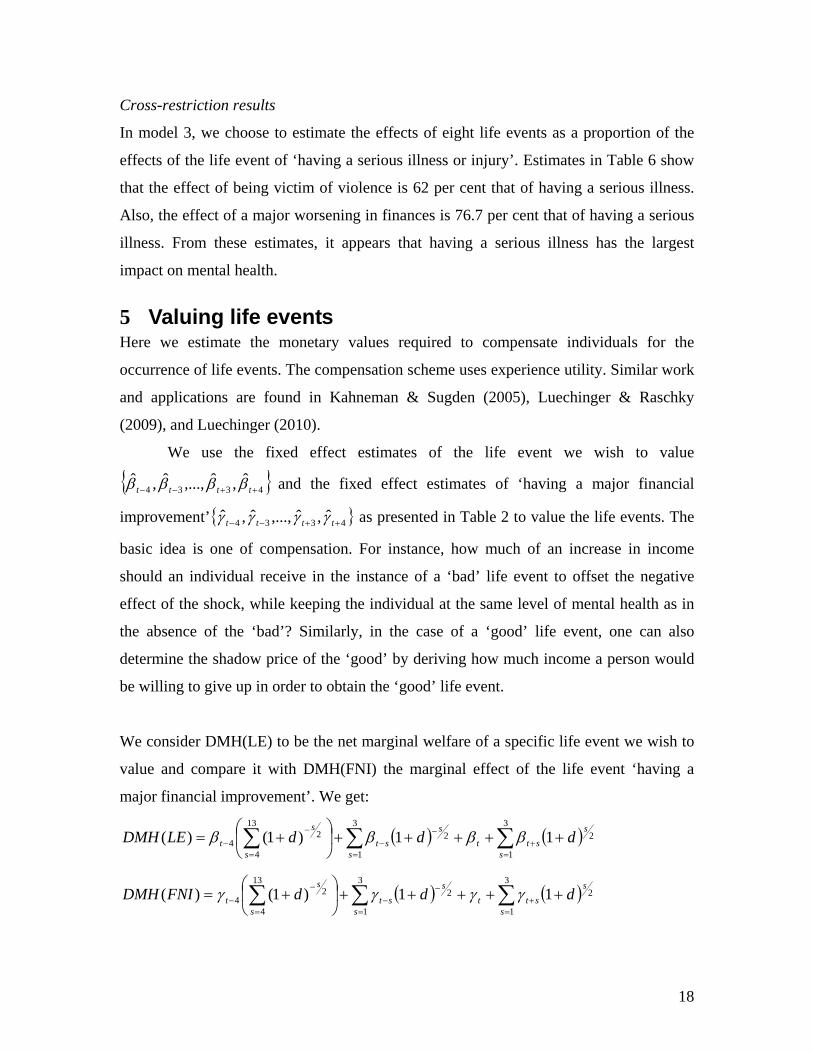
5 Valuing life events Here we estimate the monetary values required to compensate individuals for the

occurrence of life events. The compensation scheme uses experience utility. Similar work

and applications are found in Kahneman & Sugden (2005), Luechinger & Raschky

(2009), and Luechinger (2010).

We use the fixed effect estimates of the life event we wish to value

}{ 4334ˆ,ˆ,...,ˆ,ˆ++−− tttt ββββ and the fixed effect estimates of ‘having a major financial

improvement’ }{ 4334 ˆ,ˆ,...,ˆ,ˆ ++−− tttt γγγγ as presented in Table 2 to value the life events. The

basic idea is one of compensation. For instance, how much of an increase in income

should an individual receive in the instance of a ‘bad’ life event to offset the negative

effect of the shock, while keeping the individual at the same level of mental health as in

the absence of the ‘bad’? Similarly, in the case of a ‘good’ life event, one can also

determine the shadow price of the ‘good’ by deriving how much income a person would

be willing to give up in order to obtain the ‘good’ life event.

We consider DMH(LE) to be the net marginal welfare of a specific life event we wish to

value and compare it with DMH(FNI) the marginal effect of the life event ‘having a

major financial improvement’. We get:

( ) ( )∑∑∑=

+=

−−

=

−− +++++

+=

3

1

23

1

213

4

24 11)1()(

s

sstt

s

sst

s

s

t dddLEDMH ββββ

( ) ( )∑∑∑=

+=

−−

=

−− +++++

+=

3

1

23

1

213

4

24 11)1()(

s

sstt

s

sst

s

s

t dddFNIDMH γγγγ

19

( ) ( )

( ) ( )∑∑∑

∑∑∑

=+

=

−−

=

−−

=+

=

−−

=

−−

+++++

+

+++++

+

=3

1

23

1

213

4

24

3

1

23

1

213

4

24

11)1(

11)1(

)()(

s

sstt

s

sst

s

s

t

s

sstt

s

sst

s

s

t

ddd

ddd

FNIDMHLEDMH

γγγγ

ββββ

This ratio essentially indicates how many financial improvements are required to

offset another life event (Frijters, Johnston, & Shields 2011). The above compensation

scheme assumes that the estimates 4−tβ and 4−tγ reflect persistent effect on the length of

the study period (2002-2008). We do the calculations for an annual discount rate d of 10

per cent. We use the mean windfall income derived from a major improvement in

finances to assign a monetary value to these ratios. The mean windfall income for a major

financial improvement is $86,885.98 for the whole sample. Here we also calculate the

probabilities that the ratios are positive using the bootstrap method over 1,000

replications. The complement gives us the probability that the ratios are negative.

Results for valuation of life events

The estimated compensations for each life event on the whole sample and on different

sub-samples are presented in Table 3. The first column shows the discounted mental

health ratios of each event relative to that of a major financial improvement. The largest

estimate is for ‘being victim of violence’ and equals -5.599. This estimate indicates that

the mental health effect from being a victim of violence is 5.599 times larger than the

positive discounted mental health effect from a major improvement in finances.

The second column of Table 3 shows the probability that the discounted mental

health ratios are positive. As expected, the probabilities of a positive ratio when the DMH

ratio is positive is generally greater than 0.5, and the probabilities of a positive ratio when

the DMH ratio is negative is usually less than 0.5.

The last column of Table 3 shows the one-off windfall income needed to

compensate individuals for experiencing the life event under consideration. The highest

compensations required are for being a victim of violence ($486,000) and having a

serious illness ($451,000). These are the two events that had significant long run effects

on mental health and no adaptation. In the sub-samples, we find that the one-off windfall

required for constant utility increases for individuals with higher household income and is

generally greater for men than women.

20

Table 3 - Valuing life events

Life event of individual i Value(a) allFinancial improvement 1.000 86,885.98$ Serious illness - 5.198 0.131 (451,643.06)$ Friend died 0.457 0.697 39,701.20$ Victim of violence - 5.599 0.131 (486,470.08)$ Victim of crime - 1.100 0.210 (95,555.46)$ Retired - 0.988 0.250 (85,876.60)$ Fired - 1.047 0.252 (90,988.30)$ Promoted 0.837 0.802 72,699.31$ (b) Below mean HH incomeFinancial improvement 1.000 87,556.72$ Serious illness - 2.117 0.09 (982,663.08)$ Friend died 0.536 0.84 20,541.67$ Victim of violence - 1.701 0.13 (1,238,215.75)$ Victim of crime - 0.539 0.20 (210,148.39)$ Retired - 0.493 0.22 (561,590.12)$ Fired - 1.235 0.11 (42,661.71)$ Promoted 0.569 0.83 173,945.87$ (c) Above mean HH incomeFinancial improvement 1.000 86,128.70$ Serious illness - ##### 0.44 (1,141,070.05)$ Friend died - 3.992 0.38 (343,825.08)$ Victim of violence - ##### 0.42 (2,085,606.47)$ Victim of crime - 0.479 0.52 (41,224.59)$ Retired - 7.160 0.44 (616,657.12)$ Fired ##### 0.56 1,320,567.43$ Promoted 2.880 0.62 248,023.09$ (d) WomenFinancial improvement 1.000 103,219.40$ Serious illness - 4.028 0.18 (415,803.35)$ Friend died 0.534 0.56 55,151.13$ Victim of violence - 3.712 0.16 (383,198.10)$ Victim of crime - 0.822 0.32 (84,880.51)$ Retired 0.481 0.56 49,649.50$ Fired - 1.279 0.18 (132,059.31)$ Promoted 0.603 0.82 62,198.34$ (e) MenFinancial improvement 1.000 74,318.41$ Serious illness - ##### 0.366 (834,087.41)$ Friend died 0.235 0.482 17,435.83$ Victim of violence - ##### 0.369 (1,051,001.29)$ Victim of crime - 2.400 0.386 (178,374.59)$ Retired - 6.414 0.373 (476,679.40)$ Fired - 0.487 0.485 (36,211.39)$ Promoted 1.987 0.591 147,645.78$

Income shockDMH of

selfProbability for positive ratio

21

6 Further analysis To test the ‘buffering hypothesis’, we add a series of control variables in our fixed-effect

model 2. These include: being married, number of own-resident children, having lots of

friends and ability to find someone when in need of help. Table 7 presents the fixed effect

estimates of life events on mental health with the control variables. We find that all

control variables are highly significant and positive for most (e.g. married, friends and

social support) but negative for own resident children. Also estimates for the effects of

life events are usually lower when the control variables are included. This is true for the

following events: serious illness or injury, victim of crime, retirement, being fired and

worsening in finances. However, the estimates for the life events ‘victim of violence’ and

‘promoted’ are slightly larger when the control variables.

Further models

Alternatively, we can write a model that investigates by how much a form of social

support buffers against the adverse effect of a life event. We define a new least square

model for a life event k :

}{ 9,...,1*4

1

5

4,

*,

*,

5

4

*,,

*0 ∈∀+

++= ∑ ∑∑

= −=+

−=++ kuYXMH it

m stimstktm

sstkstikit βφββ

We then take the first difference to obtain the fixed-effect. We would anticipate that

0, tmφ if the variable for social support m buffers the adverse impacts of the life event

k under consideration.

The resulting sample is 57,027 person-year observations and the fixed effect

estimates are presented in Table 4. We find that the effect of serious illness on mental

health is lower for married individuals than for non-married individuals (i.e. reduced by

12 per cent) and for individuals with a larger social group (as defined by friends and

social network). Similarly, being married reduces the effects of being a victim of violence

by roughly 11 per cent and the effects of a major worsening in finances by 13 per cent.

Interestingly, having more kids in the household has no buffering effect. In some

instances, the estimate of this latter tm.,φ is positive (although insignificant),

demonstrating that having kids may worsen the effects of negative life events such as a

‘major worsening in finances’.

22

Table 4 - Cross-restrictions with control variables

Serious illness -0.120*** 0.0281 -0.0363*** -0.0494***Death of a friend 2.218 -0.160 0.665 0.912Victim of violence -0.107*** 0.0180 -0.0327*** -0.0447***Victim of crime -0.896 0.0982 -0.270 -0.371Retired -0.379 0.0816 -0.114 -0.156Promoted 0.389 -0.0619 0.117* 0.160*Fired -0.274 0.0322 -0.0822 -0.113Finances improve 0.369 -0.299 0.110 0.152Finances worsen -0.128*** 0.0266 -0.0398*** -0.0546***

N=57,027="* p<0.10 ** p<0.05 *** p<0.01"

Life events Married Kids in the household Friends Social Network

7 Concluding remarks In this paper, we have investigated the effects of nine life events on mental health using

data from seven waves (2002-08) of the Household, Income and Labour Dynamics in

Australia (HILDA) survey. The length of the panel enables us to follow the same

individual over time and to derive models that measure the adaptation and anticipation

effects of these events. This is particularly relevant when estimating implicit utility-

constant trade-offs between the experience of a given life event and a major financial

improvement.

Here, we have considered financial shocks, labour shocks, health shocks, and

social shocks. We have estimated the effects of these events on a biannual basis, up to

two year before the event occurs and up to two year after the event occurs. This enables

us to estimate the full effect of a life event and is crucial in the valuation of non-traded

goods based on experience utility.

The events that have the greatest impact in terms of mental health are having a

serious illness, a major worsening in finances, and being victim of violence. Further

analysis revealed that the effects of a major worsening in finances are roughly 77 per cent

of being seriously ill while those of being a victim of violence are around 62 per cent.

While we found complete adaptation to a major worsening in finances within 18

months and adaptation within 6 months to the following events: being a victim of crime,

being fired and being promoted, there is no evidence of adaptation to having a serious

23

illness and being victim of violence. These findings are reflected in the estimated

monetary compensation for these events. When there is full adaptation to a given event,

the income compensation for that particular event is lower than if there was no adaptation.

The largest compensations are for having a serious illness and being a victim of violence.

This shows that studies which have failed to consider anticipation and adaptation have

less than optimal results.

Finally, we found that being married reduces the effects of having a serious illness

by 12 per cent and the effects of a major worsening in finances by almost 13 per cent.

Acknowledgements “This paper uses unit record data from the Household, Income and Labour Dynamics in Australia (HILDA) Survey. The HILDA Project was initiated and is funded by the Australian Government Department of Families, Housing, Community Services and Indigenous Affairs (FaHCSIA) and is managed by the Melbourne Institute of Applied Economic and Social Research (Melbourne Institute). The findings and views reported in this paper, however, are those of the author and should not be attributed to either FaHCSIA or the Melbourne Institute.”

References

Almgren, G., Magarati, M., & Mogford, L. (2009). "Examining the influences of gender, race, ethnicity, and social capital on the subjective health of adolescents." Journal of Adolescence

Bergensen, H., Froslie, K., Sunnerhagen, K., & Schanke, A. (2010). "Anxiety, Depression, and Psychological Well-being 2 to 5 years Poststroke."

32: 109-133.

Journal of Stroke and Cerebrovascular Diseases

Blanchflower, D., & Oswald, ,A. (2008). "Hypertension and happiness across nations."

19(5): 364.

Journal of Health EconomicsBoes, S., & Winkelmann, R. (2004). Income and Happiness: New results from

Generalized Threshold and Sequential Models.

27: 218-233.

Working Paper No. 0407

Brazier, J., Roberts, J., & Deverill, M. (2002). "The estimation of a preference-based measure of health from the SF-36."

, University of Zurich. Socioeconomic Institute.

Journal of Health EconomicsBridges, S., & Disney, R. (2010). "Debt and depression."

21: 271-292. Journal of Health Economics

Butterworth, P., Rodgers, B., & Windsor, T. (2009). "Financial hardship, socio-economic position and depression: Results from the PATH Through Life Survey."

28: 388-403.

Social Science and Medicine 69: 229-237.

24

Clark, A., Diener, E., Geogellis, Y., & Lucas, R. (2008). "Lags and Leads in life satisfaction: A test of the baseline approach." Economic Journal

Cohen, M. (2008). "The effect of crime on life satisfaction." 118: F222-F239.

Journal of Legal Studies

Contonyannis, P., Jones, A., & Rice, N. (2004). "The dynamics of health in the British Household Panel Survey."

37: S325.

Journal of Applied EconometricsCornwell, E., & Waite, L. (2009). "Social disconnectedness, perceived isolation, and

health among older adults."

19: 473-503.

Journal of Health and Social Behavior

Diener, E., & Oishi, S. (2000). Money and Happiness: Income and Subjective Well-Being Across Nations.

50(March): 31-48.

Culture and Subjective Well-being

Dolan, P., Peasgood, T., & White, M. (2008). "Do we really know what makes us happy? A review of the economic literature on the factors associated with subjective well-being."

. E. Diener, Suh, E., The MIT Press: 185-218.

Journal of Economic PsychologyEasterlin, R. (2001). "Income and happiness: Towards a unified theory."

29: 94-122. The Economic

JournalEasterlin, R., & Plagnol, A. (2008). "Life satisfaction and economic conditions in East

and West Germany pre- and post-unification."

111(473): 465-484.

Journal of Economic Behaviour & Organization

Fletcher, A., & Shaw, R. (2000). "Sex differences in associations between parental behaviors and characteristics and adolescent social integration."

68: 433-444.

Social Development

Frey, B., & Stutzer, A. (2002). 9(2): 133-148.

Happiness and EconomicsFrijters, P., Johnston, D., & Shields, M. (2011). "Life Satisfaction Dynamics with

Quarterly Life Event Data."

, Princeton University Press.

Scandinavian Journal of EconomicsGardner, J., & Oswald, A. (2007). "Money and mental wellbeing: A longitudinal study of

medium-sized lottery wins."

113(1): 190-211.

Journal of Health EconomicsGreen, F. (2010). "Unpacking the misery multiplier: how employability modifies the

impacts of unemployment and job insecurity on life satisfaction and mental health."

26: 49-60.

Journal of Health EconomicsJoutsenniemi, K., Martelin, T., Martikainen, P., Pirkola, S., & Koskinen, S. (2006).

"Living arrangements and mental health in Finland."

.

Journal of Epidemiology and Community Health

Kahneman, D., & Sugden, R. (2005). "Experienced utility as a standard of policy evaluation."

60: 468-475.

Environmental & Resource EconomicsLee, R., & Robbins, S. (1998). "The relationship between social connectedness, anxiety,

self-esteem and social identity."

32: 161-181.

Journal of Counselling Psychology

Luechinger, S. (2010). "Life satisfaction and transboundary air pollution."

45(3): 338-345.

Economics Letters

Luechinger, S., & Raschky, P. (2009). "Valuing flood disasters using the life satisfaction approach."

107: 4-6.

Journal of Public EconomicsLund, R., Due, P., Modvig, J., Holstein, B., Damsgaard, T., & Andersen, P. (2002).

"Cohabitation and marital status as predictors of mortality an eight year follow-up study."

93: 620-633.

Social Science and MedicineMandal, B., Ayyagari, P., & Gallo, W. (2010). "Job loss and depression: The role of

subjective expectations."

55(4): 673-679.

Social Science and Medicine xxx(1-8).

25

Oswald, A., & Gardner, J. (2006). "Do divorcing couples become happier by breaking up?" Journal of the Royal Statistical Society. Series A

Oswald, A., & Powdthavee, N. (2008a). "Death, happiness, and the calculations of compensatory damages."

169: 319-336.

Journal of Legal StudiesOswald, A., & Powdthavee, N. (2008b). "Does happiness adapt? A longitudinal study of

disability with implications for economists and judges."

37: S217.

Journal of Public Economics

Powdthavee, N. (2009). "What happens to people before and after disability? Focusing effects, lead effects, and adaptation to different areas of life."

92: 1061-1077.

Social Science and Medicine

Tan, M. (2007). The effects of family cohesion and personality on the mental health of young Australians, ANU.

69: 1834-1844.

Vinck, P., & Pham, P. (2010). "Association of exposure to violence and potential traumatic events with self-reported physical and mental health status in the Central African Republic." Journal of The American Medical Association

Ware, J. (2007). "SF-36 Health Survey Update." Retrieved 27th July 2010, from

304(5): 544-552.

http://www.sf-36.org/tools/sf36.shtml. Waxler-Morrison, N., Hislop, G., Mears, B., Kan, L. (1991). "Effects of social

relationships on survival for women with breast cancer: A prospective study." Social Science and Medicine

Wyke, S., & Ford, G. (1992). "Competing explanations for associations between marital status and health."

33(2): 177-183.

Social Science and Medicine Zimmermann, A., & Easterlin, R. (2006). "Happily ever after? Cohabitation, marriage,

divorce, and happiness in Germany."

34(5): 523-532.

Population and Development Review

32: 511-528.

26

Appendix

Table 5 - OLS estimates of the effect of life events on mental health

<-24 -20.46*** (-20.62) 0.755 (0.83) -19.97*** (-9.90) -2.485** (-2.30) 0.211 (0.12) 1.132 (0.78) 3.288***(2.92) 6.758*** (5.06) -23.72*** (-15.28)-18 to -24 -28.75*** (-16.98) -4.469*** (-2.62) -21.77*** (-5.51) -6.104*** (-2.67) -10.57*** (-3.36) -1.534 (-0.54) 2.836 (1.31) 8.374*** (3.06) -18.86*** (-6.51)-12 to -18 -17.91*** (-11.80) -2.259* (-1.77) -24.44*** (-7.49) -5.081*** (-2.88) 7.880** (2.12) 0.130 (0.05) 0.431 (0.27) 4.230* (1.83) -24.91*** (-9.21)-6 to -12 -40.90*** (-27.49) -5.551*** (-3.70) -32.43*** (-9.72) -5.986*** (-2.90) -14.91*** (-5.35) -3.050 (-1.20) 4.408** (2.32) 4.207* (1.72) -39.51*** (-15.45)0 to -6 -44.29*** (-33.50) -4.254*** (-3.79) -38.37*** (-13.71) -7.917*** (-5.07) 5.005 (1.52) -4.833** (-2.25) 5.254***(3.78) 3.281 (1.59) -43.94*** (-19.18)

Next 6 mths -15.60*** (-10.31) -1.963 (-1.53) -20.00*** (-5.82) -7.519*** (-4.07) 12.07*** (3.16) -0.746 (-0.29) 5.047***(3.16) 1.357 (0.57) -26.56*** (-9.87)Next 6-12 mths -26.05*** (-15.19) -1.231 (-0.71) -20.49*** (-4.90) -2.488 (-0.99) -11.80*** (-3.69) -12.86*** (-4.22) 4.084* (1.87) 0.367 (0.13) -16.62*** (-5.47)Next 12-18mths -11.88*** (-6.80) 0.423 (0.29) -22.53*** (-5.41) -7.706*** (-3.48) 6.922 (1.64) 1.826 (0.61) 1.119 (0.61) 1.594 (0.58) -20.67*** (-6.62)Next 18-24mths -12.56*** (-6.31) 1.577 (0.79) -9.521* (-1.87) -2.744 (-0.87) -0.103 (-0.03) -8.764** (-2.40) 2.185 (0.87) -5.186 (-1.60) -14.93*** (-4.17)

24months+ -11.41*** (-9.17) 3.652*** (3.26) -11.55*** (-3.90) -0.953 (-0.57) 6.145*** (2.70) -1.459 (-0.69) 1.265 (0.91) 2.778 (1.55) -15.67*** (-7.60)

Years of education 2.476*** (16.07)Age 0.0438 (0.56)Age sq./100 -0.256*** (-3.13)

N =74,003t statistics in parentheses* p < 0.10, ** p < 0.05, *** p < 0.01

Victim of violence

Additional variables

6-month period Serious illness or injury Death of a friend Finances worsenVictim of crime Retired Fired Promoted Finances improve

27

Table 6 - Cross-restrictions on the vector of parameters

<-24 -3.727** (-2.34)-18 to -24 -5.874*** (-3.78)-12 to -18 -4.586*** (-2.95)-6 to -12 -21.07*** (-12.21)0 to -6 -29.61*** (-17.43)

Next 6 mths -2.602* (-1.66)Next 6-12 mths -8.158*** (-4.81)Next 12-18mths 1.347 (0.98)Next 18-24mths 2.714* (1.77)

RestrictionsSerious illnessDeath of a friend 0.0338 (1.16)Victim of violence 0.623*** (7.95)Victim of crime 0.101** (2.49)Retired 0.0598 (0.81)Fired 0.0677 (1.24)Promoted -0.0645* (-1.74)Finances improve -0.0379 (-0.75)Finances worsen 0.767*** (11.71)

N = 57,027t statistics in parentheses* p<0.10 ** p<0.05 *** p<0.01

Time periods Serious illness of violence

28

Table 7 - Fixed effects estimates with control variables of social network

<-24 -6.870*** (-5.88) 2.055* (1.92) -4.376 (-1.64) -1.284 (-0.85) -0.945 (-0.41) -0.330 (-0.17) 0.900 (0.69) 3.385* (1.92) -2.943 (-1.51)-18 to -24 -10.67*** (-7.69) -1.507 (-1.10) -6.314* (-1.83) -0.379 (-0.20) -5.078* (-1.95) 1.600 (0.67) 1.148 (0.67) 3.981* (1.77) -2.651 (-1.11)-12 to -18 -6.471*** (-4.99) -0.193 (-0.18) -6.358** (-2.17) -0.595 (-0.37) 0.261 (0.08) -0.758 (-0.35) -0.173 (-0.13) 4.369** (2.16) -6.717*** (-2.91)-6 to -12 -22.25*** (-17.09) -2.228* (-1.73) -20.27*** (-6.28) -1.526 (-0.82) -7.776*** (-3.20) -1.238 (-0.54) 1.480 (0.92) 1.806 (0.85) -23.08*** (-10.34)0 to -6 -31.02*** (-25.76) -1.014 (-1.00) -22.47*** (-8.16) -5.029*** (-3.32) 2.403 (0.84) -4.079** (-1.99) 3.911*** (3.08) 1.883 (1.01) -24.44*** (-11.69)

Next 6 mths -2.548** (-2.00) 0.272 (0.25) -8.122*** (-2.71) -3.994** (-2.45) 1.211 (0.39) -0.811 (-0.37) 3.962*** (2.94) 0.448 (0.22) -8.228*** (-3.66)Next 6-12 mths -10.78*** (-7.68) -0.693 (-0.50) -10.80*** (-3.04) -0.225 (-0.11) -9.753*** (-3.74) -9.998*** (-3.94) 1.629 (0.93) -1.766 (-0.77) -3.957 (-1.61)Next 12-18mths 1.170 (0.83) 1.887 (1.61) -7.496** (-2.20) -4.634** (-2.55) -2.775 (-0.84) 2.621 (1.08) 0.182 (0.12) -0.0749 (-0.03) 0.920 (0.37)Next 18-24mths 1.779 (1.14) 0.372 (0.24) -3.540 (-0.87) 0.704 (0.29) 2.072 (0.72) -6.131** (-2.13) 0.577 (0.30) -5.390** (-2.13) -3.272 (-1.17)

No. yrs of education 0.868 (1.61)Age 3.035*** (7.08)Age sq./100 -2.307*** (-7.16)No. own resident children -1.659*** (-3.01)Married 4.655*** (4.18)Friend 3.725*** (20.61)Social support 4.841*** (27.60)

N =74,003t statistics in parentheses

Promoted

Control variables:

6-month periodSerious illness or

injury Death of a friend Victim of violence

* p < 0.10, ** p < 0.05, *** p < 0.01

Finances improve Finances worsen

Additional variables:

Victim of crime Retired Fired