JRER Vol. 34 No. 3 – 2012 The Estimation and Determinants of the Price Elasticity of Housing Supply: Evidence from China Authors Songtao Wang, Su Han Chan, and Bohua Xu Abstract This paper provides a first look at estimates of the price elasticity of the housing supply in China at both the national and city levels. Using a panel dataset consisting of 35 cities in China from 1998 to 2009, the findings show that the implied national price elasticity of housing supply is between 2.8 and 5.6. The city- level analysis reveals that geographic, economic as well as regulatory factors are significant determinants of the variation in the observed price elasticity of housing supply. The study of a different regulatory and economic environment contributes to the growing literature on supply elasticity and helps explain the seemingly wide variation in supply elasticities observed across cities and countries. The rapid growth in housing prices in many cities around the world since the late 1990s has motivated a growing number of studies (Jud and Winkler, 2002; Glaeser, Gyourko, and Saiz, 2008; Goodman and Thibodeau, 2008; Wheaton and Nechayev, 2008; and Shi, Young, and Hargreaves, 2010) to examine the variation in housing price dynamics across cities or regions. Although strong economic growth and intensified housing financial support along with other demand-side factors may have played a role in the recent run-up in housing prices, these demand-side factors alone are insufficient to capture the variations in the regional price dynamics. Hence, an increasing number of supply-side studies have started to surface to shed light on the role housing supply plays in housing price dynamics. One focus of such housing supply studies is on estimating the price elasticity of housing supply, a parameter that measures the responsiveness of housing supply to a change in housing price. This parameter is important for housing market and policy analyses as it has implications to the relation between house price fluctuations and demand shocks. The magnitude of housing price changes as well as the time taken to restore a new level of price equilibrium due to an unexpected shock in housing demand are greatly affected by the price elasticity of housing supply. Prior studies used different models to analyze data at the national or city
Transcript
J R E R � V o l . 3 4 � N o . 3 – 2 0 1 2
T h e E s t i m a t i o n a n d D e t e r m i n a n t s o f t h e
P r i c e E l a s t i c i t y o f H o u s i n g S u p p l y :
E v i d e n c e f r o m C h i n a
A u t h o r s Songtao Wang, Su Han Chan, and Bohua Xu
A b s t r a c t This paper provides a first look at estimates of the price elasticityof the housing supply in China at both the national and citylevels. Using a panel dataset consisting of 35 cities in China from1998 to 2009, the findings show that the implied national priceelasticity of housing supply is between 2.8 and 5.6. The city-level analysis reveals that geographic, economic as well asregulatory factors are significant determinants of the variation inthe observed price elasticity of housing supply. The study of adifferent regulatory and economic environment contributes to thegrowing literature on supply elasticity and helps explain theseemingly wide variation in supply elasticities observed acrosscities and countries.
The rapid growth in housing prices in many cities around the world since the late1990s has motivated a growing number of studies (Jud and Winkler, 2002; Glaeser,Gyourko, and Saiz, 2008; Goodman and Thibodeau, 2008; Wheaton andNechayev, 2008; and Shi, Young, and Hargreaves, 2010) to examine the variationin housing price dynamics across cities or regions. Although strong economicgrowth and intensified housing financial support along with other demand-sidefactors may have played a role in the recent run-up in housing prices, thesedemand-side factors alone are insufficient to capture the variations in the regionalprice dynamics. Hence, an increasing number of supply-side studies have startedto surface to shed light on the role housing supply plays in housing pricedynamics.
One focus of such housing supply studies is on estimating the price elasticity ofhousing supply, a parameter that measures the responsiveness of housing supplyto a change in housing price. This parameter is important for housing market andpolicy analyses as it has implications to the relation between house pricefluctuations and demand shocks. The magnitude of housing price changes as wellas the time taken to restore a new level of price equilibrium due to an unexpectedshock in housing demand are greatly affected by the price elasticity of housingsupply. Prior studies used different models to analyze data at the national or city
3 1 2 � W a n g , C h a n , a n d X u
level over selected time periods, finding a wide range of empirical estimates ofthis supply parameter. However, there is yet to be a consensus on the method toestimate the price elasticity of housing supply. In addition, the bulk of the evidencefocuses on the housing market in the United States, with only limited evidenceon non-U.S. markets.
In general, the literature on supply elasticity addresses two related researchquestions. The first concerns the extent to which supply elasticity impacts housingprice dynamics. Prior studies on this issue (Wheaton, 2005; Glaeser, Gyourko,and Saks, 2008; and Grimes and Aitken, 2010) generally confirm an inverserelationship, that is, a more elastically supplied housing market tends to have lowerprice levels as well as smaller price volatilities than a market with less elasticsupply. The second question concerns the sources of variation in the estimatedprice elasticity of housing supply across different countries (Mayo and Sheppard,1996; Malpezzi and Mayo, 1997; Malpezzi and Maclennan, 2001; and Vermeulenand Rouwendal, 2007) or different cities/regions within a country (Harter-Dreiman, 2004; and Green, Malpezzi, and Mayo, 2005). However, while some ofthe papers include one or two factors (regulatory, economic, and geographic) intheir analyses, none of them analyzed all the three factors simultaneously.
The aim of this study is twofold. First, it seeks to estimate an aggregate or nation-wide price elasticity of the housing supply in China to throw light on thecomparative responsiveness of the housing supply in China relative to othercountries. Second, it seeks to estimate the price elasticity of the housing supplyat the city-level as well as identify the key determinants of variations in housingsupply responsiveness across cities/regions in China. An examination of theregulatory, economic, and geographic related factors may help shed light on therelative importance of the factors in explaining differences in housing supplyelasticity.
China, similar to the U.S., exhibits significant local variation in land availability,population density, infrastructure, and regulatory practices. However, it is anemerging economy with a recently liberalized private housing market. Its supplyenvironment is unique in that all urban land in China is collectively owned by thepeople through the National People’s Congress of the People’s Republic of China.The central as well as the local governments in China exert a strong influence onthe development process through the timing of land supply [see Lai and Wang(1999) and Chan, Fang, and Yang (2011) for a discussion of land supply policieson developers’ housing supply strategies]. In addition, the prevalent use of apresale system in China to sell development projects is a unique featureinfluencing the supply decisions of developers [see Lai, Wang, and Zhou (2004),Chan, Fang, and Yang (2008, 2012), and Fang, Wang, and Yang (2012) for adiscussion of this issue]. Given the above unique features of China, the currentstudy certainly adds a new dimension to the international comparative literatureon housing supply elasticity as well as provides additional insights into theunderlying forces shaping the heterogeneous housing supply responsiveness acrosscities or regional markets. The latter results may have implications to thedifferential house price sensitivities to demand shocks observed across cities.
P r i c e E l a s t i c i t y o f H o u s i n g S u p p l y � 3 1 3
J R E R � V o l . 3 4 � N o . 3 – 2 0 1 2
This study examines the 35 largest cities in China (most of which are provincialcapital cities) over a 12-year period from 1998 to 2009. Using a modified versionof Malpezzi and Maclennan’s (2001) stock adjustment model to estimate theaggregate price elasticity of supply, we find that the estimated elasticity for Chinafalls in the range of 2.82 to 5.64. Relative to other countries, this estimate putsChina in a moderately elastic supply category together with postwar U.S. andprewar U.K. The estimate for China is lower than that for countries with liberalregulatory environments (such as prewar U.S. and Thailand) but higher than thatfor countries with stringent regulatory environments (such as postwar U.K., theNetherlands, Korea, and Malaysia). The finding adds to existing evidence thatseems to indicate that the price elasticity of supply is correlated with the stringencyof the regulatory environment.
Further, we directly estimate the price elasticity of the housing supply at the citylevel [as in Green, Malpezzi, and Mayo (2005) and Grimes and Aitken (2010)]and explore the sources of variation in those estimates across the 35 cities inChina, finding the key determinants to be the availability of developable land, theaverage urban built-up area, the growth rate of population, and the regulatoryrestrictions on land use and/or land supply. Of those determinants, geographicalconstraint affecting the availability of developable land seems to be the mostimportant. Overall, the findings help enrich our understanding of China’s housingmarket from the supply side and fill a gap in the literature on China’s housingmarket that, in general, has largely overlooked housing supply elasticity as anexplanatory variable in housing price dynamics.
The remainder of the paper is organized as follows. The next section provides abrief overview of China’s evolving housing market, followed by a review of therelated literature in section three. Section four discusses the estimation model, thedata, and the estimates for the national price elasticity of housing supply. Sectionfive estimates city-level housing supply elasticities, identifies their determinants,and discusses the results, while the final section concludes.
� A B r i e f O v e r v i e w o f C h i n a ’s H o u s i n g M a r k e t
The replacement of the welfare housing system in China in 1998 with one that ismarket-oriented has led to a gradual release of pent-up demand for privatehousing. Over the decade from 1998 to 2009, the number of new immigrants tothe major cities in China grew substantially and the rate of urbanization increasedfrom 30% to about 47%. Under such demand shifts and a booming economy,many of the urban housing markets across China experienced a sustained priceincrease. The average price appreciation rates over this period were 36%, 24%,and 20% in the East, West, and Central regions, respectively.1 It is noteworthythat throughout the period, housing price levels in the East were substantiallyhigher than the national average and the levels in the West and Central regions.
Such price appreciations occurred despite the fact that, in mid-2003, the centralgovernment of China began to launch a wide range of regulatory policies
3 1 4 � W a n g , C h a n , a n d X u
(including mortgage and reserve rates adjustments, tax rate adjustments, housingprice regulation, land-use rights transaction reform and supply structure regulation)to restrain the rising residential prices (see Wang and Yang, 2010).2 The supply-side policy measures, in particular, are aimed at improving housing supplyresponsiveness to demand shocks as well as providing more affordable housingfor low and medium income households. Given that demand-side regulations werefound to have rather limited effects in curbing house price appreciations,increasing attention has shifted to supply-side policies in the later years.
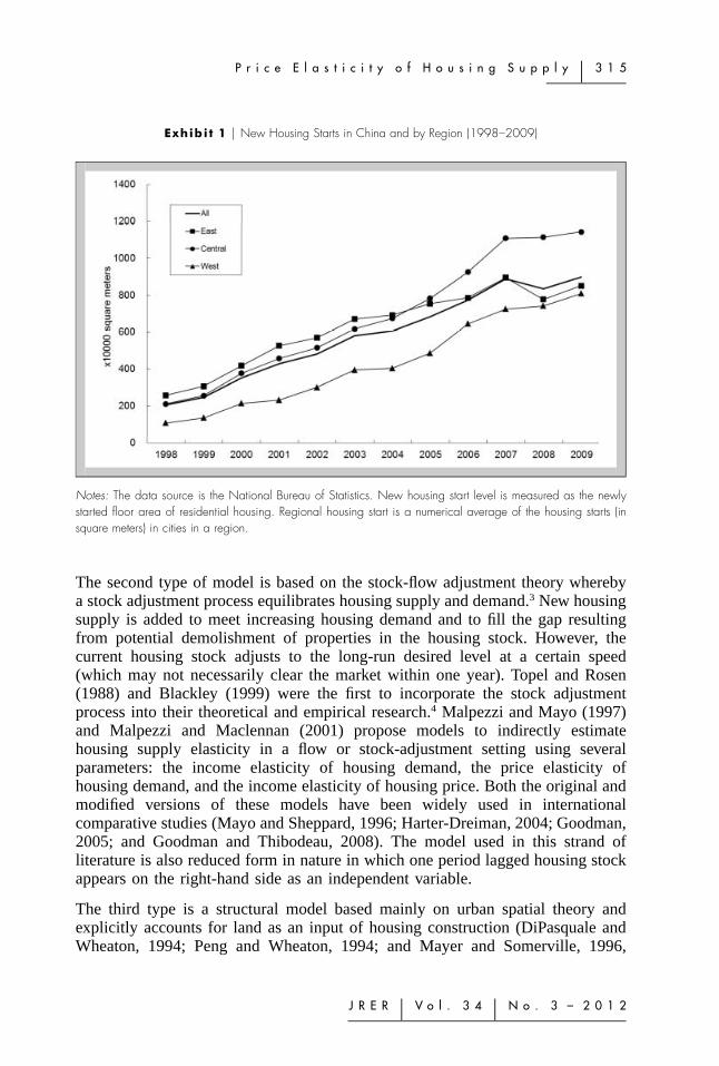
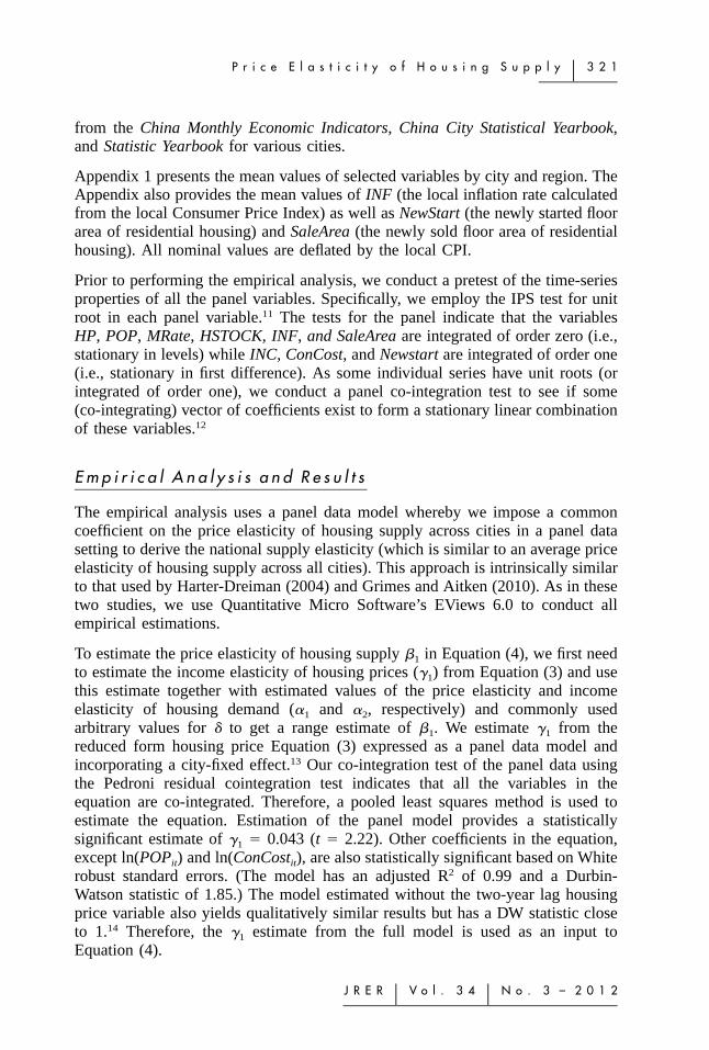
While price appreciation rates differ across regions, new housing supply alsoexhibits distinctive trends across regions during the 1998 to 2009 period (Exhibit1). Of note is the general increase in housing starts across all regions over theperiod, with the level of housing starts in the East consistently higher than theCentral and West regions up until around 2004, after which the levels in the Eastfell below that of the Central region and began to approach that of the West.Recognizing that variations in housing supply would likely be larger across citiesthan across regions, our prior is that such variations are possibly correlated withthe regulatory, economic and geographic features unique to each region/city.
� P r i o r R e s e a r c h o n H o u s i n g S u p p l y E l a s t i c i t y
There is a growing literature on housing supply elasticity focusing mainly on theU.S. housing market with only a handful of studies examining non-U.S. housingmarkets. These studies, however, vary in their estimation methods and produce awide range of supply elasticities (Kim, Phang, and Wachter, 2012). To date,although there is a fair degree of agreement on the fundamental factors affectinghousing supply, there is yet to be a consensus as to which estimation method ofthe price elasticity of supply is best. The reason could be related to problems withdata availability and aggregation bias in the data (DiPasquale, 1999; and Harter-Dreiman, 2004). This section reviews the estimation methods used in the literatureand the results obtained.
E s t i m a t i o n M e t h o d s
Prior studies use one of three main types of models, each involving differenteconometric techniques, to estimate the price elasticity of housing supply (anumerical measure of the responsiveness of the housing supply to a change inhousing price). The first type is based on the Tobin’s q theory, which posits thatthe level of housing investment is a positive function of the ratio of housing pricesto construction costs. Studies using this approach include Muth (1960), Follain(1979), Green, Malpezzi, and Mayo (2005), Vermeulen and Rouwendal (2007),and Grimes and Aitken (2010). Most of empirical settings in the above studiesare reduced form equations with price and cost shifters (typically, land cost,material cost, labor cost, and various interest costs) on the right-hand side.
P r i c e E l a s t i c i t y o f H o u s i n g S u p p l y � 3 1 5
J R E R � V o l . 3 4 � N o . 3 – 2 0 1 2
Exhibi t 1 � New Housing Starts in China and by Region (1998–2009)
Notes: The data source is the National Bureau of Statistics. New housing start level is measured as the newlystarted floor area of residential housing. Regional housing start is a numerical average of the housing starts (insquare meters) in cities in a region.
The second type of model is based on the stock-flow adjustment theory wherebya stock adjustment process equilibrates housing supply and demand.3 New housingsupply is added to meet increasing housing demand and to fill the gap resultingfrom potential demolishment of properties in the housing stock. However, thecurrent housing stock adjusts to the long-run desired level at a certain speed(which may not necessarily clear the market within one year). Topel and Rosen(1988) and Blackley (1999) were the first to incorporate the stock adjustmentprocess into their theoretical and empirical research.4 Malpezzi and Mayo (1997)and Malpezzi and Maclennan (2001) propose models to indirectly estimatehousing supply elasticity in a flow or stock-adjustment setting using severalparameters: the income elasticity of housing demand, the price elasticity ofhousing demand, and the income elasticity of housing price. Both the original andmodified versions of these models have been widely used in internationalcomparative studies (Mayo and Sheppard, 1996; Harter-Dreiman, 2004; Goodman,2005; and Goodman and Thibodeau, 2008). The model used in this strand ofliterature is also reduced form in nature in which one period lagged housing stockappears on the right-hand side as an independent variable.
The third type is a structural model based mainly on urban spatial theory andexplicitly accounts for land as an input of housing construction (DiPasquale andWheaton, 1994; Peng and Wheaton, 1994; and Mayer and Somerville, 1996,
3 1 6 � W a n g , C h a n , a n d X u
2000a, 2000b). Poterba (1984) and Saiz (2010) are two other studies thatincorporate land into their housing supply estimation.
In the above studies, housing starts (or changes in the stock of housing, net ofremovals), new residential constructions or housing permit issuances are generallyused as a measure of new housing supply (a flow variable). However, in the modelto estimate the price elasticity of housing supply, some studies specify thevariables in levels (e.g., Topel and Rosen, 1988; Malpezzi and Maclennan, 2001;and Grimes and Aitken, 2010) while others specify the variables in differences(e.g., Mayer and Somerville, 2000b; and Goodman and Thibodeau, 2008).
Mayer and Somerville (2000b) argue that, since housing price is a stock variablewhile new housing supply is a flow variable, it is proper to use price change (aflow variable) to explain the dynamics of housing supply. (Note that this argumentfocuses on the time-series properties of the data to avoid spurious regression.)Grimes and Aitken (2010), however, justify the use of a price levels modelingapproach by pointing out that the existence of a co-integration relationshipbetween housing supply and its explanatory variables should be the keyconsideration rather than how the variables are specified. Hence, it is necessaryto perform a co-integration test on the variables to check the appropriateness oftheir specification in the model.
E m p i r i c a l E s t i m a t e s o f t h e P r i c e E l a s t i c i t y o f H o u s i n gS u p p l y
With different models, econometric techniques, data (national or MSA level), andtime periods used, prior studies generate a wide range of estimates for the priceelasticity of housing supply. At the national level, Muth (1960), using a reducedform model, finds that the U.S. has highly elastic housing supply between theFirst and the Second World Wars. Follain (1979), using data from 1947 to 1975,obtains a similar estimation of high elasticity for the U.S. However, Poterba(1984), using a structural asset-market model data from 1963 to 1982, obtains anestimate between 0.5 and 2.9. Topel and Rosen (1988) find a short-run (one-quarter) and longer-run supply elasticity of 1.0 and 3.0, respectively, but note thatmost of the difference vanishes within one year. DiPasquale and Wheaton (1994),using an urban spatial model and U.S. data from 1963 to 1990, find an elasticityestimate ranging from 1.0 to 1.2 for new housing construction and 1.2 to 1.4 forhousing stock, while Blackley (1999), using 1950 to 1994 U.S. data, obtainsestimates ranging from 1.6 to 3.7 for new residential constructions. Malpezzi andMaclennan (2001) obtain estimates ranging from 4 to 10 (prewar) and 6 to 13(postwar) using a flow model and estimates ranging from 1 to 6 (postwar) usinga stock adjustment model.
More recently, Harter-Dreiman (2004) uses a VEC model to estimate housingsupply elasticities for 76 MSAs in the U.S. and finds the range to be from 1.8 to3.2. Green, Malpezzi, and Mayo (2005) also find a wide distribution of supply
P r i c e E l a s t i c i t y o f H o u s i n g S u p p l y � 3 1 7
J R E R � V o l . 3 4 � N o . 3 – 2 0 1 2
elasticity estimates for 45 U.S. cities, with the city-level estimates ranging from�0.30 to 29.9. Goodman (2005), using data on 317 U.S. suburban areas in the1970s, 1980s, and 1990s, obtains supply elasticity estimates in the range of 1.26to 1.42 while Goodman and Thibodeau (2008), examining 133 U.S. MSAs from1990 to 2000, find the range to be from �1.37 to 2.98. Saiz (2010), usingtopographically-derived estimates of developable land ratio along with the localregulation data from the literature, obtains housing supply elasticity estimates inthe range of 0.6 to 5.45 for 95 U.S. MSAs.
In addition, several studies estimate the housing supply elasticity for countriesoutside the U.S. For the U.K., Malpezzi and Maclennan (2001) find the elasticityestimate based on a flow model to be between 1 and 4 (prewar) and between 0and 1 (postwar) and the estimate based on a stock adjustment model to be between0 and 0.5 (postwar). Mayo and Sheppard (1996) find Malaysia’s supply elasticityto be between 0 and 1.5, Korea’s to be between 1 and 1.5, and Thailand’s to benear infinite. In another study, Malpezzi and Mayo (1997) find Malaysia’s supplyelasticity to be between 0 and 0.35, Korea’s to be between 0 and 0.17, andThailand’s to be near infinite. Peng and Wheaton (1994) find the supply elasticityto be 1.1 in Hong Kong while Vermeulen and Rouwendal (2007) find zeroelasticity in the Netherlands, both in the short run and the long run.
In summary, the above studies offer a wide range of estimates on housing supplyelasticity across different countries and even for the same country. This variationmay be attributed partially to differences in methodologies employed and partiallyto differences in regulatory, economic, and/or geographic features unique to eachcountry or city.
S o u r c e s o f Va r i a t i o n
A large number of the studies exploring the sources of differences in housingsupply elasticities across countries or cities focus on the relative stringency ofregulatory policies on land and housing development in those countries or cities.These studies use a variety of regulation indices [such as that from Gyourko, Saiz,and Summers (2008)], the number of governing bodies, the number of regulationpolicies, months to receive subdivision approval, the number of growthmanagement policies instituted by a local authority or a development fee(Manning, 1996; Mayer and Somerville, 2000a; Green, Malpezzi, and Mayo,2005; and Quigley and Raphael, 2005). Generally, these studies find a statisticallysignificant negative effect of regulatory stringency on housing supply elasticity.In addition, Green, Malpezzi, and Mayo (2005) find that factors such as populationdensity, population levels, population change, and house price levels are alsoimportant in influencing regional/city-level housing supply elasticity.
To date, Saiz (2010) is the only study in the literature that uses satellite-generateddata on terrain elevation and the presence of water bodies to testify that physicalland constraint (in addition to regulatory constraint) is important in explaining
3 1 8 � W a n g , C h a n , a n d X u
housing supply elasticity. Saiz proposes a model that links geography with housingsupply directly through constraints on land availability and indirectly throughregulatory constraints, the latter of which are endogenous to prices and pastgrowth. His main finding is that the amount of undevelopable land in U.S.metropolitan areas is a key factor impacting housing supply elasticity in the areasexamined.
From these studies, it is evident that regulatory, economic, and geographic factorsaffect the supply elasticity of housing. To date, however, no research has examinedthe impact of all the three groups of factors simultaneously on housing supplyelasticity. This paper fills this gap and examines the influence of these threefactors, as well as their relative importance, in determining the price elasticitiesof housing supply across China’s urban cities.
� A g g r e g a t e E s t i m a t e o f t h e P r i c e E l a s t i c i t y o f H o u s i n g� S u p p l y i n C h i n a
T h e M o d e l a n d E m p i r i c a l S p e c i f i c a t i o n s
The model for estimating the price elasticity of housing supply at the aggregatedlevel builds upon the simple stock adjustment model presented by Malpezzi andMaclennan (2001). However, the accuracy of the estimates of supply elasticityalso hinges on the specification of the reduced-form house price equation andestimates of the demand elasticities (Meen, 2005; and Kim, Phang, and Wachter,2012). To address this issue, we embellish the Malpezzi and Maclennan (2001)model to include a real cost of homeownership variable in the demand equationto capture its influence on housing demand, two period lagged housing prices inthe supply equation to examine the possibility of lags in the housing supplyadjustment given a lengthy housing construction process, and construction costand capital cost in the housing supply equation given that both are importantindicators influencing the housing supply decision.5
The embellished version of Malpezzi and Maclennan’s (2001) stock adjustmentmodel is as follows:
Q � �(K* � K )dt t t�1
K* � � � � HP � � INC � � POP � � OwnCostt 0 1 t 2 t 3 t 4 t
Q � � � � HP � � HP � � HP � � ConCostst 0 1 t 2 t�1 3 t�2 4 t
� � MRate5
Q � Q (1)dt st
P r i c e E l a s t i c i t y o f H o u s i n g S u p p l y � 3 1 9
J R E R � V o l . 3 4 � N o . 3 – 2 0 1 2
where, Qd (Qs) is the log quantity of housing demanded (supplied), K* is the logof the desired housing stock, Kt�1 is the log of the housing stock in the previousperiod, and � is the housing stock adjustment per period. In this setting, Qd is afunction of the difference between the desired stock and the stock in the previousperiod. HP is the log of the price level of standard housing, INC is the log ofurban household disposable income per capita, POP is the log of total residentialpopulation, OwnCost is the cost of home ownership, ConCost is the log ofconstruction cost, and MRate is the mortgage interest rate that serves as a proxyfor the development loan rate in the supply equation. The t subscript denotes year.As in Malpezzi and Maclennan (2001), we interpret the coefficients as elasticities.Therefore, �1 is the price elasticity of housing supply.
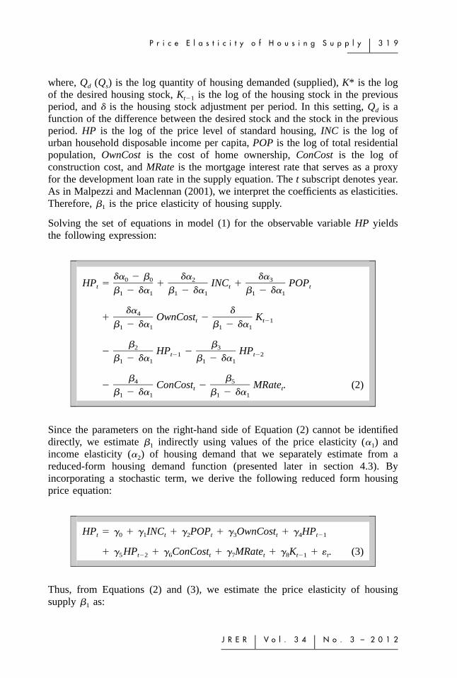
Solving the set of equations in model (1) for the observable variable HP yieldsthe following expression:
Since the parameters on the right-hand side of Equation (2) cannot be identifieddirectly, we estimate �1 indirectly using values of the price elasticity (�1) andincome elasticity (�2) of housing demand that we separately estimate from areduced-form housing demand function (presented later in section 4.3). Byincorporating a stochastic term, we derive the following reduced form housingprice equation:
HP � � � � INC � � POP � � OwnCost � � HPt 0 1 t 2 t 3 t 4 t�1
� � HP � � ConCost � � MRate � � K � � . (3)5 t�2 6 t 7 t 8 t�1 t
Thus, from Equations (2) and (3), we estimate the price elasticity of housingsupply �1 as:
3 2 0 � W a n g , C h a n , a n d X u
�2� � � � � , (4)� �1 1�1
where �1 is the estimated elasticity of housing price with respect to income and� is the parameter of stock adjustment speed that can be assigned artificially (asin prior studies). A higher (lower) � would imply a more (less) responsiveenvironment in which a larger (smaller) portion of the gap between the desiredand actual stock will be filled through the construction process. Malpezzi andMaclennan (2001) set the parameter value of � in their stock adjustment modelfor the U.S. and the U.K. as 0.3 or 0.6, depicting a moderate speed of adjustment.Note that a � value of one would imply that the gap is fulfilled within a singleperiod, which is the assumption underlying the flow model used by Mayo andSheppard (1996), Malpezzi and Mayo (1997), and Malpezzi and Maclennan(2001).6 Given the likelihood of construction lags in the housing market, the mainresults we report are based on the stock adjustment model.
D a t a S o u r c e s a n d D e s c r i p t i o n
The data covers macro-economic indicators as well as housing market variablesin 35 major Chinese cities from 1998 to 2009. Due to the limited length of time-series data available, major cities are pooled to create a panel dataset thatcomprises of 35 cross-sections over a 12-year period, with a total count of 420observations for each pooled variable.
HP (housing price level) is calculated using the Real Estate Price Index of 35major cities published by the National Bureau of Statistics and the NationalDevelopment and Reform Commission.7 This index is transaction-based and isthe best available annual housing price data in China for its wide coverage ofsample cities as well as its length.8 HSTOCK (housing stock K) is estimated bymultiplying per capita floor area and residential population in the year 1999. Weuse 1999 because the China City Statistical Yearbook only reports the averagefloor area in 1999 and in some other selected years. Using the newly completedfloor area in each year as the flow amount, the housing stock in each of thefollowing years is estimated accordingly.9
INC is the urban household disposable income per capita and POP is the totalresidential population. MRate is a five-year lending rate, which we use to proxyfor the development loan rate. It can also serve as a proxy for OwnCost (the realcost of homeownership) if we ignore expected housing price appreciation.10 Thus,for our empirical analysis, we use MRate in place of OwnCost in Equation (3).Lastly, ConCost (the construction cost of housing development) is measured bydividing the material costs of completed housing units by the annual completedfloor area. Thus this measure serves as a rough proxy of structure cost (excludingland and labor costs). The data for INC, POP, MRate, and ConCost are sourced
P r i c e E l a s t i c i t y o f H o u s i n g S u p p l y � 3 2 1
J R E R � V o l . 3 4 � N o . 3 – 2 0 1 2
from the China Monthly Economic Indicators, China City Statistical Yearbook,and Statistic Yearbook for various cities.
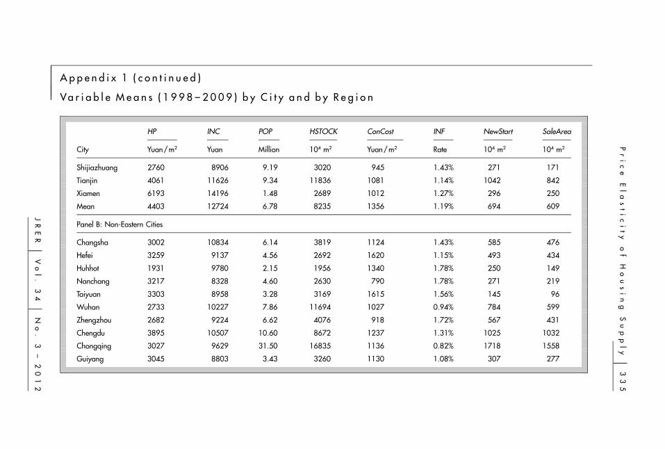
Appendix 1 presents the mean values of selected variables by city and region. TheAppendix also provides the mean values of INF (the local inflation rate calculatedfrom the local Consumer Price Index) as well as NewStart (the newly started floorarea of residential housing) and SaleArea (the newly sold floor area of residentialhousing). All nominal values are deflated by the local CPI.
Prior to performing the empirical analysis, we conduct a pretest of the time-seriesproperties of all the panel variables. Specifically, we employ the IPS test for unitroot in each panel variable.11 The tests for the panel indicate that the variablesHP, POP, MRate, HSTOCK, INF, and SaleArea are integrated of order zero (i.e.,stationary in levels) while INC, ConCost, and Newstart are integrated of order one(i.e., stationary in first difference). As some individual series have unit roots (orintegrated of order one), we conduct a panel co-integration test to see if some(co-integrating) vector of coefficients exist to form a stationary linear combinationof these variables.12
E m p i r i c a l A n a l y s i s a n d R e s u l t s
The empirical analysis uses a panel data model whereby we impose a commoncoefficient on the price elasticity of housing supply across cities in a panel datasetting to derive the national supply elasticity (which is similar to an average priceelasticity of housing supply across all cities). This approach is intrinsically similarto that used by Harter-Dreiman (2004) and Grimes and Aitken (2010). As in thesetwo studies, we use Quantitative Micro Software’s EViews 6.0 to conduct allempirical estimations.
To estimate the price elasticity of housing supply �1 in Equation (4), we first needto estimate the income elasticity of housing prices (�1) from Equation (3) and usethis estimate together with estimated values of the price elasticity and incomeelasticity of housing demand (�1 and �2, respectively) and commonly usedarbitrary values for � to get a range estimate of �1. We estimate �1 from thereduced form housing price Equation (3) expressed as a panel data model andincorporating a city-fixed effect.13 Our co-integration test of the panel data usingthe Pedroni residual cointegration test indicates that all the variables in theequation are co-integrated. Therefore, a pooled least squares method is used toestimate the equation. Estimation of the panel model provides a statisticallysignificant estimate of �1 � 0.043 (t � 2.22). Other coefficients in the equation,except ln(POPit) and ln(ConCostit), are also statistically significant based on Whiterobust standard errors. (The model has an adjusted R2 of 0.99 and a Durbin-Watson statistic of 1.85.) The model estimated without the two-year lag housingprice variable also yields qualitatively similar results but has a DW statistic closeto 1.14 Therefore, the �1 estimate from the full model is used as an input toEquation (4).
3 2 2 � W a n g , C h a n , a n d X u
We estimate �1 and �2 from a reduced-form housing demand function as specifiedbelow:
ln(SaleArea ) � � � � ln(HP ) � � ln(INC ) � � ln(POP )it 0 1 it 2 it 3 it
� � MRate � � FE � � FE � � ,4 it 5i i 6t t it (5)
where SaleAreait is the sold floor area in city i at year t, which serves as a proxyfor housing demand. FEi is a city-fixed effect, FEt is a year-fixed effect, and �it
is the error term for city i at year t. The other independent variables (in city i atyear t) are as previously defined.15 There are 420 observations (35 cities over 12years: 1998–2009). Estimation of Equation (5) using a pooled least squaresmethod provides statistically significant estimates of �1 � �0.765 (t � �4.94)and �2 � 0.437 (t � 3.04). The coefficients, �3 and �4, are also statisticallysignificant based on White standard errors.
It is noteworthy that the estimated values of �1 and �2 lie within the rangesassumed in the literature. Malpezzi and Maclennan (2001) assume �1 and �2 tobe in the intervals (�0.5, �0.1) and (0.5, 1), respectively, for the U.S. and theU.K. Mayo and Sheppard (1996) assume �1 and �2 lie in the interval (�0.2, �0.5)and (0.5, 1), respectively, for Malaysia, Korea, and Thailand while Malpezzi andMayo (1997) assume �1 and �2 lie in the interval (�0.5, �1) and (1, 1.5),respectively, for the same three countries.
Using the estimated value of �1 (0.043), the estimated values of �1 and �2 (�0.765and 0.437, respectively) and arbitrary values of � [set as 0.3 and 0.6 followingMalpezzi and Maclennan, (2001)], we find from Equation (4) the implied priceelasticity of supply �1 to be 2.82–5.64.16 Alternatively, using assumed values of�1 and �2 from Malpezzi and Mayo (1997) and Malpezzi and Maclennan (2001),we obtain estimates of �1 of 3.3–13.9.
As a robustness check, we estimate an alternative model similar to the factor price-excluded reduced form housing price model used in Malpezzi and Maclennan(2001). This model has ln(HP) as the dependent variable and only ln(INC),ln(POP), and ln(Kt�1) as explanatory variables. We estimate the model withCochrane–Orcutt correction (including both AR(1) and AR(2) to eliminate serialcorrelation).17 The estimation yields �1 � 0.091 while the estimated �1 and �2 are�0.901 and 0.482, respectively. Setting � to be 0.3 and 0.6, the implied priceelasticity of the housing supply �1 is 1.32–2.64.18 �1 is 1.5–6.5 using assumedvalues from Malpezzi and Mayo (1997) and Malpezzi and Maclennan (2001).Estimates from this alternative model are generally lower than those derived fromthe embellished model.
Exhibit 2 compares the elasticity estimates with that of other countries, whilerecognizing the broad ranges and imprecision of the estimates. Given that we
Pr
ic
eE
la
st
ic
it
yo
fH
ou
si
ng
Su
pp
ly
�3
23
JR
ER
�V
ol
.3
4�
No
.3
–2
01
2
Exhibi t 2 � Comparison of Supply Elasticity Estimates Across Countries
Countries Period Data Source Elasticity Estimate Category
U.S. Prewar National Malpezzi and Maclennan (2001) 4.40�10.40 (flow) ElasticPostwar �1994 National Malpezzi and Maclennan (2001) 5.60�12.70 (flow) ElasticPostwar �1994 National Malpezzi and Maclennan (2001) 1.20�5.60 (stock) Moderately Elastic
U.K. Prewar National Malpezzi and Maclennan (2001) 1.40�4.30 (flow) Moderately ElasticPostwar �1995 National Malpezzi and Maclennan (2001) 0.00�0.50 (flow) InelasticPostwar �1995 National Malpezzi and Maclennan (2001) 0.00�0.50 (stock) Inelastic
Korea 1970�1986 National Malpezzi and Mayo (1997) 0.00�0.17 (flow) Inelastic
Malaysia 1970�1986 National Malpezzi and Mayo (1997) 0.07�0.35 (flow) Inelastic
Thailand 1970�1986 National Malpezzi and Mayo (1997) � (flow) Highly Elastic
China 1998�2009 Aggregatedacross cities
This paper 2.82�5.64 (stock)5.96 (flow)
Moderately Elastic
Notes: Flow stands for flow model while stock stands for stock adjustment model.
3 2 4 � W a n g , C h a n , a n d X u
derived our aggregate elasticity estimate for China using the stock adjustment (aswell as flow) models, Exhibit 2 only reports the comparative estimates fromstudies that use either of those two models. Studies (not reported in Exhibit 2)that use alternative estimation methods obtain a supply elasticity estimate of 1.1for Hong Kong (Peng and Wheaton, 1994), near zero for the Netherlands(Vermeulen and Rouwendal, 2007), 0–0.84 for the U.K. (Meen, 2008), and 0.01for New Zealand (Grimes and Aitken, 2010).
Comparing across countries (Exhibit 2), the price elasticity of the housing supplyin China in 1998–2009 appears to be moderate and somewhat in line with thesituation in postwar U.S. and prewar U.K. At the extremes, Thailand exhibits ahighly elastic housing supply environment while Korea, Malaysia, and postwarU.K. exhibit inelastic housing supply. The Netherlands and New Zealand (notshown in Exhibit 2) also exhibit inelastic housing supply.
Prior comparative studies (Mayo and Sheppard, 1996; Malpezzi and Mayo, 1997;and Malpezzi and Maclennan, 2001) attribute the substantial variations in supplyelasticities across countries to restrictive land use policies. Such internationalvariations in supply elasticities and their correlation to regulatory practices holdtrue across cities in the U.S. as well (Green, Malpezzi, and Mayo, 2005). Theimplication of these findings is that the regulatory environment is an importantdeterminant of the spatial variation in supply responsiveness.
� C i t y - S p e c i f i c E s t i m a t e s a n d t h e i r D e t e r m i n a n t s
In this section we estimate supply elasticities at the city-level and identify theirsources of variations. Note that cities across China exhibit significant localvariation in topology, housing market maturity, and regulatory practices. Theanalysis proceeds in two stages. We first estimate the price elasticity of supplyfor each of the 35 cities using a variable-coefficient panel data model. In thesecond stage, we analyze their determinants by regressing the estimated supplyelasticities on a set of explanatory variables.
S t a g e I A n a l y s i s a n d R e s u l t s
To estimate the city-level supply elasticity, we estimate new housing starts inresponse to changes in housing prices, while controlling for important cost shiftersin a panel data model. The stock adjustment model (that we use to estimatenational-level supply elasticity) has two limitations if used for estimating supplyelasticity at the city-level. The first is the need to estimate or assign a speed ofstock adjustment parameter � for each city in order to obtain a point estimate(rather than a range of estimates) of supply elasticity for our cross-sectionalregression analysis. (The point estimates of different cities are used as dependentvariables in stage II.) Given that the speed of adjustment is affected by marketfundamentals, which vary greatly across cities, it is unrealistic to impose an
P r i c e E l a s t i c i t y o f H o u s i n g S u p p l y � 3 2 5
J R E R � V o l . 3 4 � N o . 3 – 2 0 1 2
identical � for all cities or to artificially assign a value for � to estimate the supplyelasticity of a city. Second, the length of the dataset (12 observations for eachcity) relative to the number of explanatory variables makes the stock adjustmentmodel unsuitable for estimating city-level supply elasticity.19
Using the panel data set of 420 observations (35 cities over 12 years: 1998–2009),we estimate the price elasticity of supply at the city-level using a panel data model[as in Grimes and Aitken (2010)]. The equation is specified as follows:
� � ln(ConCost ) � � MRate � � FE � � ,3 it 4 it 5i i it (6)
where the variables (in city i at year t) are as previously defined. �0 is an overallconstant term, �1i is the price elasticity of supply for city i, �5i incorporates cityfixed-effects for city i, and �it is the error term. The coefficients of ConCost,MRate, and HPt�1 are restricted to be identical across cities.20 Hence, the equationhas only one unrestricted coefficient, �1i, which reflects city-specific conditions.In other words, not only the intercepts would vary with city, the slope for ln(HPit)would also vary according to the city.21 Given the short time series, we assumeno significant temporal effects and, therefore, do not include a year-fixed effectin the model to conserve degrees of freedom in the estimation. The inclusion ofa one-year lagged housing price variable in the model is consistent with thehousing supply specification in Equation (1) and also helps alleviate theautocorrelation problem.22 The inclusion of cost shifters (ConCost and MRate) inthe housing supply equation is in line with prior studies (Topel and Rosen, 1988;Mayer and Somerville, 2000; and Meen, 2005).23
As before, a pretest of the panel data reveals that there is at least one co-integratedvector between the pooled variables in the equation. We estimate equation (6) bypooled least squares with White period standard errors, which are robust to serialcorrelation within cross-section and time-varying variances in the disturbances,and report the estimation results in Exhibit 3. (In Section 5.2, we discuss theresults of a robustness check where we estimate the model using instrumentalvariables to address potential errors in variables problem as well as potentialendogeneity problem between housing supply and housing prices.)24
As Panel A of Exhibit 3 shows, the signs of the coefficients of ConCost andMRate are in line with expectations. Panel B presents the key estimate, �1i, whichis the price elasticity of housing supply for city i. As the panel shows, all butthree cities—Beijing, Shenzhen, and Kunming—exhibit significantly positiveprice elasticity of housing supply estimates.25 The elasticity estimate isinsignificant and close to zero for Beijing and Shenzhen while that for Kunmingis significantly negative. The estimate for Shanghai is a low (but significantlypositive) 1.52. It is noteworthy that Beijing, Shenzhen, and Shanghai (the three
3 2 6 � W a n g , C h a n , a n d X u
Exhibi t 3 � Housing Supply Elasticity Estimates by City
Panel A: Estimates for Control Variables
Variable Coefficient
ln (HPt�1) �1.61**
ln (ConCost) �0.07
MRate �7.10***
Panel B: Estimates of the Price Elasticity of Housing Supply by City (�1i)
City Elasticity Estimate City Elasticity Estimate
Xining 37.05*** Tianjin 5.10***
Yinchuan 21.98*** Lanzhou 4.90***
Changsha 17.14*** Wuhan 4.66***
Urumqi 16.71*** Chongqing 4.51***
Zhengzhou 16.50*** Dalian 4.41***
Hefei 13.03*** Chengdu 4.36***
Guangzhou 12.62*** Fuzhou 3.85***
Nanning 11.45*** Xiamen 3.47***
Guiyang 9.71*** Nanjing 3.42***
Huhhot 9.63*** Qingdao 2.89***
Taiyuan 9.16*** Jinan 2.68***
Haikou 8.83*** Hangzhou 2.65***
Xi’an 8.04*** Ningbo 2.27***
Shijiazhuang 7.89*** Shanghai 1.52**
Nanchang 6.78*** Beijing 0.53
Harbin 6.30*** Shenzhen 0.49
Shenyang 5.75*** Kunming �7.70***
Changchun 5.40***
Panel C: Statistics
Adj. R2 0.88 F-Statistics 40.78***
Notes: The table reports results from the estimation equation:
ln(NewStart ) � � � � ln(HP ) � � ln(HP ) � � ln(ConCost ) � � MRate � � FE � � .it 0 1i it 2 i,t�1 3 it 4 it 5i i it
Equation is estimated using a pooled least squares method. City-fixed effects are included butnot reported. There are 385 observations (35 cities over 11 years: 1999–2009). Statisticalsignificance tests are based on White period standard errors. Cities in italics are the Eastern cities.**Significant at the 5% level.***Significant at the 1% level.
P r i c e E l a s t i c i t y o f H o u s i n g S u p p l y � 3 2 7
J R E R � V o l . 3 4 � N o . 3 – 2 0 1 2
biggest housing sub-markets in China in terms of existing housing stock) exhibitrather large housing price appreciations but relatively small increases in housingstarts during the sample period. At the extremes are Kunming (in the Westernregion) and Xining (in the Central region) with elasticity estimates of �7.70 and37.05, respectively. Kunming is the only city in the sample experiencing a negativereal housing price change (�4.6%) from 1998 to 2009 while Xining’s phenomenalgrowth in housing development is fueled by the central government’s ‘‘Go West’’development policy implemented in early 2000 rather than by a change in demandfor housing. Thus, we treat Kunming and Xining as outliers and exclude themfrom the stage II regression analysis.
The overall mean of the 33 city-level supply elasticity estimates (excludingKunming and Xining) reported in Exhibit 3 is a significant 7.23 (t � 7.90).[Interestingly, this mean estimate is close to the mean of the 45 U.S. city-levelsupply elasticity estimates reported by Green, Malpezzi, and Mayo (2005), whoalso used a direct estimation approach to estimate the price elasticity of supply atthe city-level.] A univariate comparison of the mean supply elasticities betweenthe 18 Eastern cities and the 15 non-Eastern cities reveals that the housing supplyresponsiveness of the Eastern sub-group (mean elasticity � 4.45) is about halfthat of the non-Eastern sub-group (mean elasticity � 10.57). This difference insupply responsiveness may well reflect the difference in economic and regulatoryfeatures associated with Eastern versus non-Eastern cities. Generally, Eastern citiesare economically more vibrant (with higher income and higher housing pricelevels) and have a more mature housing market (with a higher level of housingstocks) than non-Eastern cities (Appendix 1). In addition, the housing markets inthe Eastern cities are generally subject to more stringent governmental regulations.
S t a g e I I A n a l y s i s a n d R e s u l t s
The Empirical Model and Data. In this section we identify the sources of variationin supply elasticities across cities. We regress the estimated city-level supplyelasticities on a set of explanatory variables classified under one of threecategories: geographic, economic, and regulatory. The full regression model (withcity-specific proxy variables from each category) is:
� � � � � DevelopableLandRatio � � EAST1i 0 1 i 2 i
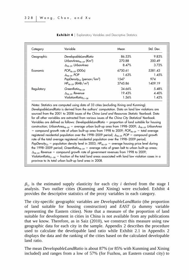
Notes: Statistics are computed using data of 33 cities (excluding Xining and Kunming).DevelopableLandRatio is derived from the authors’ computation. Data on land law violations aresourced from the 2001 to 2008 issues of the China Land and Resources Statistic Yearbook. Datafor all other variables are extracted from various issues of the China City Statistical Yearbook.Variables are defined as follows: DevelopableLandRatio � proportion of land suitable for housingconstruction; UrbanArea98–09 � average urban built-up area from 1998–2009; �98–09 UrbanArea� compound growth rate of urban built-up area from 1998 to 2009; POP98–09 � total averageregistered residential population over the 1998–2009 period; �98–09 POP � compound growthrate of the total average registered residential population over the 1998–2009 period;PopDensity03 � population density level in 2003; HP98–09 � average housing price level duringthe 1998–2009 period; GreenRatio98–09 � average ratio of green belt to urban built-up areas;�98–09 Revenue � compound growth rate of government revenues from 1998 to 2009;ViolationRatio01–08 � fraction of the total land areas associated with land law violation cases in aprovince to its total urban built-up land area in 2008.
�1i is the estimated supply elasticity for each city i derived from the stage Ianalysis. Two outlier cities (Kunming and Xining) were excluded. Exhibit 4provides the descriptive statistics of the proxy variables in each category.
The city-specific geographic variables are DevelopableLandRatio (the proportionof land suitable for housing construction) and EAST (a dummy variablerepresenting the Eastern cities). Note that a measure of the proportion of landsuitable for development in cities in China is not available from any publicationsthat we know. Therefore, as in Saiz (2010), we construct this measure using rawgeographic data for each city in the sample. Appendix 2 describes the procedureused to calculate the developable land ratio while Exhibit 2.1 in Appendix 2displays the data and the ranking of the cities based on the calculated developableland ratio.
The mean DevelopableLandRatio is about 87% (or 85% with Kunming and Xiningincluded) and ranges from a low of 57% (for Fuzhou, an Eastern coastal city) to
P r i c e E l a s t i c i t y o f H o u s i n g S u p p l y � 3 2 9
J R E R � V o l . 3 4 � N o . 3 – 2 0 1 2
a high of 99% (for Yinchuan, a Central inland city). From Exhibit 3, Fuzhou hasa housing supply elasticity estimate (3.85) that is about half that of the samplemean (7.23) while Yinchuan’s estimate (21.98) is the second highest among the35 cities. This observation conforms somewhat to our expectation of a positivecorrelation between the ratio of developable land and the price elasticity ofhousing supply.
The next six variables in the model are city-specific economic variables.UrbanArea98–09 is the average urban built-up area and �98–09 UrbanArea isthe annual compound growth rate of urban built-up area from 1998 to 2009.POP98–09 and �98–09 POP are the total average registered residential populationand its annual compound growth rate, respectively, over the 1998–2009 period.PopDensity03 is the population density level in 2003.26 HP98–09 is the averagehousing price level during the 12-year period. Data for these economic variablesare extracted from various issues of the China City Statistical Yearbook.
Generally, a city with a larger built-up urban area will have a lower potential landsupply. Thus we would expect that as an urban built-up area increases, housingsupply elasticity falls. Similarly, as the growth rate of urban built-up area rises,we would expect that the price elasticity of the housing supply falls. Followingthe theoretical model presented in Green, Malpezzi, and Mayo (2005), as thepopulation of a city rises, the price elasticity of supply falls and as housing pricesrise, so does the supply elasticity. However, as the authors note, the latter tworelationships are somewhat ambiguous given the possibility of two-way causalflows between housing supply elasticity and the two variables. The rate ofpopulation growth, however, may influence builders’ expectations and hence theirsupply decisions. Therefore, it is reasonable to expect that as population growthrate increases, so does supply responsiveness.
The last three variables are the city-specific regulatory variables. GreenRatio98–09
is the average ratio of greenbelt to urban built-up areas. �98–09 Revenue is thecompound growth rate of government revenues from 1998 to 2009 andViolationRatio01–08 is the fraction of the total land areas associated with land lawviolation cases in a province to its total urban built-up land area in 2008. Datafor the green ratio and government revenues are extracted from various issues ofthe China City Statistical Yearbook while data on land law violations in eachprovince are sourced from the 2001–2008 issues of the China Land and ResourcesStatistic Yearbook. Since there is no regulation index constructed for China, weuse these three variables to proxy for government restrictions on land use andland transactions in each city. Generally, we would expect that as governmentrestrictions on land use or land supply rises, housing supply elasticity falls.
The green ratio is part of a city’s urban development policy. Although it may bepossible to convert the usage of greenbelts to increase the supply of land fordevelopment, the political cost of such conversions could be rather high. As such,we would expect that as the green ratio rises, less land will be available fordevelopment and, hence, housing supply elasticity falls. The growth in municipal
3 3 0 � W a n g , C h a n , a n d X u
government revenues (�98–09 Revenue) may serve as an indicator of governmentrestrictions on land supply given that revenues from land granting comprise alarge share of the total government revenues. (For example, in 2009, China’sgovernment revenues from land granting comprise about 21% of the totalrevenues.) Thus, a higher growth in government revenues would imply lowergovernment restrictions on land supply and, hence, higher supply elasticity. Theincidence of land law violations (ViolationRatio01–08) serves as an indicator ofgovernment restrictions on land transactions. Thus, a higher violation ratio wouldimply lower government restrictions and, hence, higher housing supply elasticity.
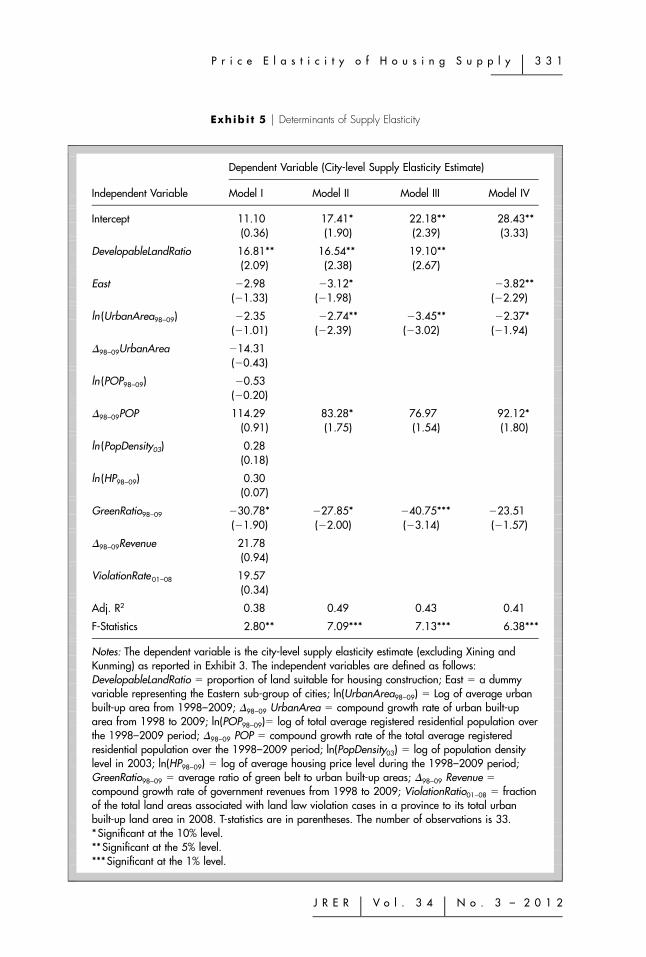
Regression Results. Exhibit 5 presents the results from four specifications of theregression model (7).27 Model I incorporates all the variables specified in Equation(7), while the other three models include only selected explanatory variables fromeach of the three categories.
The Model I results show that only DevelopableLandRatio and GreenRatio98–09
have a statistically significant relationship with supply elasticity and in thedirection conforming to our expectations. Model II excludes selected insignificantvariables and shows an improved adjusted R2 over Model I. In this model, anadditional three variables (East, urban built-up area, and population growth rate)are statistically significant and display their predicted signs. Excluding the Eastvariable from Model II reduces the adjusted R2 of the model from 49% to 43%and population growth rate becomes statistically insignificant, as shown in theModel III result. Instead, when DevelopableLandRatio is excluded from ModelII, the adjusted R2 of the model drops even further (from 49% to 41%) and theGreenRatio98–09 becomes insignificant, as shown in Model IV result. The latterresult lends some support to Saiz’s (2010) finding that geography is a keydeterminant of housing supply elasticity.
We also perform a robustness check by generating a new set of supply elasticityestimates from an alternative specification of Equation (6) and use them asdependent variables in Equation (7). Specifically we estimate Equation (6) usinga two-stage least squares approach in a panel data setting (as in Grimes andAitken, 2010), whereby a one-year lagged (log) population, lagged (log) income,and lagged mortgage rate serve as instruments for the concurrent (log) housingprice while the other exogenous variables serve as their own instrumentalvariables. The results (in terms of relative ranking of the cities based on theirestimated supply elasticities) from the above specifications are qualitatively similarto those in Exhibit 3. Re-running Equation (7) using elasticity estimates from thisspecification shows DevelopableLandRatio, East, and UrbanArea98–09 to besignificant explanatory variables (adjusted R2 of model � 38.4%). Excluding Eastfrom the regression model, DevelopableLandRatio, GreenRatio98–09, POP98–09, andHP98–09 are significant explanatory variables (adjusted R2 of model � 36.5%).Note that in comparison to Model II in Exhibit 5, these models have a muchlower adjusted R2, although the overall results are generally in line with that inModel II.
P r i c e E l a s t i c i t y o f H o u s i n g S u p p l y � 3 3 1
Notes: The dependent variable is the city-level supply elasticity estimate (excluding Xining andKunming) as reported in Exhibit 3. The independent variables are defined as follows:DevelopableLandRatio � proportion of land suitable for housing construction; East � a dummyvariable representing the Eastern sub-group of cities; ln(UrbanArea98–09) � Log of average urbanbuilt-up area from 1998–2009; �98–09 UrbanArea � compound growth rate of urban built-uparea from 1998 to 2009; ln(POP98–09)� log of total average registered residential population overthe 1998–2009 period; �98–09 POP � compound growth rate of the total average registeredresidential population over the 1998–2009 period; ln(PopDensity03) � log of population densitylevel in 2003; ln(HP98–09) � log of average housing price level during the 1998–2009 period;GreenRatio98–09 � average ratio of green belt to urban built-up areas; �98–09 Revenue �compound growth rate of government revenues from 1998 to 2009; ViolationRatio01–08 � fractionof the total land areas associated with land law violation cases in a province to its total urbanbuilt-up land area in 2008. T-statistics are in parentheses. The number of observations is 33.*Significant at the 10% level.**Significant at the 5% level.***Significant at the 1% level.
3 3 2 � W a n g , C h a n , a n d X u
To summarize, the main regression result (based on Model II of Exhibit 5)suggests that generally cities in the non-Eastern region and those with higherdevelopable land ratios, less built-up urban areas, higher population growth rates,and less restrictive land use regulations (as evidenced by a lower green ratio)display higher price elasticities of housing supply. The findings on populationgrowth and land use regulation are consistent with Green, Malpezzi, and Mayo(2005), who examine regulatory and economic factors as potential determinantsof supply elasticities across 45 U.S. cities.
It is important to note that the empirical results demonstrate that geographic,economic, and regulatory factors determine housing supply elasticity across cities.If this also holds true across countries, then the large variance in supply elasticityobserved across countries could be a reflection of underlying differences in thegeographic, economic, and regulatory environments in the different countries.
We estimated the average developable land ratio for 35 China’s urban cities to bearound 85%, which is higher than the 74% estimated by Saiz (2010) for U.S.metro areas.28 Therefore, on average, China’s cities seem to be less landconstrained than U.S. cities, which would imply that China’s supply environmentshould be more price elastic than that of the U.S. (holding other factors constant).However, regulatory and economic factors may also be at work. Compared to theU.S., China has more restrictive policies for housing and land transactions andalso displays a more rapid rate of growth of built-up urban areas during the periodexamined. Therefore, considering all factors—geographic, regulatory, andeconomic—together, we find China’s price elasticity of supply to be moderatelyelastic and somewhat in line with that in the U.S. Similar analysis could beextended to explain the variations in supply elasticities between other countriesas well.
Note that the findings also have implications to our comprehension of the leveland volatility of house prices observed in cities across China. Casual observationinforms us that many of the cities in China that exhibit high house priceappreciations are associated with low supply responsiveness (e,g., Beijing,Shanghai, and Shenzhen). Analyzing our data on 33 cities (excluding Kunmingand Xining), we find a negative correlation of about 0.49 between the meanhousing price level (from Appendix 1) and the housing supply elasticity in eachcity (from Exhibit 3).
� C o n c l u d i n g R e m a r k s
Using data on 35 major cities in China, we estimate the price elasticities ofhousing supply at both the aggregated and city levels, as well as identify thefactors that matter in determining supply elasticity. The findings reveal that, at theaggregated level, China’s housing supply is moderately elastic (somewhat in linewith postwar U.S. and prewar U.K.) but is less (more) price elastic than countrieswith liberal (highly restrictive) regulatory environments.
P r i c e E l a s t i c i t y o f H o u s i n g S u p p l y � 3 3 3
J R E R � V o l . 3 4 � N o . 3 – 2 0 1 2
The analysis at the city-level reveals that geographical constraint, the averagebuilt-up urban area, the rate of population growth, and regulatory restrictions onland use matter in determining housing supply elasticities. These determinants,some of which are in line with past research, shed light on the reasons for thevariations in housing supply responsiveness across cities and possibly acrosscountries as well.
We calculate a developable land ratio from satellite-generated data for each of the35 major cities in China and confirm a positive and significant relationshipbetween the availability of developable land and housing supply elasticity. Thisgeographical factor is also found to be one of the most important determinants ofthe price elasticity of housing supply. This finding suggests that housing supplyelasticity is determined not only by housing market factors (such as built-up urbanareas, house price levels, and regulatory constraints), but also by factors (such aspre-existing geographical constraints) that are exogenous to the housing market.This result should serve to motivate future studies to link geography to housing-related issues.
One shortcoming of our study is the limited length of the time-series data availableon China. As more data become available, future studies could test the stabilityof the estimated parameters over a longer time horizon that encompasses upturnsand downturns in the economy.
33
4�
Wa
ng
,C
ha
n,
an
dX
u
� A p p e n d i x 1�� Va r i a b l e M e a n s ( 1 9 9 8 – 2 0 0 9 ) b y C i t y a n d b y R e g i o n
HP INC POP HSTOCK ConCost INF NewStart SaleArea
City Yuan/m2 Yuan Million 104 m2 Yuan/m2 Rate 104 m2 104 m2
� A p p e n d i x 1 ( c o n t i n u e d )�� Va r i a b l e M e a n s ( 1 9 9 8 – 2 0 0 9 ) b y C i t y a n d b y R e g i o n
HP INC POP HSTOCK ConCost INF NewStart SaleArea
City Yuan/m2 Yuan Million 104 m2 Yuan/m2 Rate 104 m2 104 m2
Kunming 2877 8910 4.94 4164 1204 1.91% 382 426
Lanzhou 2562 7719 3.05 2583 1239 1.13% 149 128
Nanning 2639 9479 6.49 2660 1131 1.19% 306 291
Urmuqi 2775 9072 1.91 3001 976 1.13% 175 243
Xian 3747 9480 7.23 5591 1408 0.71% 494 448
Xining 2031 7194 1.96 1432 1211 2.03% 88 70
Yinchuan 2538 7998 1.28 1633 1041 1.77% 136 161
Mean 2899 9134 6.33 4698 1185 1.38% 463 414
Notes: The data sources are various issues of China Monthly Economic Indicators, the China City Statistical Yearbook, and the Statistic Yearbook of differentcities. Data shown are in nominal values. HP is the price level of standard housing service, INC is the urban household disposable income per capita, POP isthe total residential population, HSTOCK is housing stock, ConCost is the construction cost, INF is the local inflation rate calculated from the local ConsumerPrice Index, NewStart is the newly started floor area of residential housing, and SaleArea is the newly sold floor area of residential housing.
P r i c e E l a s t i c i t y o f H o u s i n g S u p p l y � 3 3 7
J R E R � V o l . 3 4 � N o . 3 – 2 0 1 2
� A p p e n d i x 2�� C o m p u t i n g t h e D e v e l o p a b l e L a n d R a t i o o f 3 5 C h i n a� C i t i e s
As in Saiz (2010), we process satellite-generated data on terrain elevation andpresence of water bodies to precisely estimate the amount of developable land ineach Chinese city. We use the ASTER Global Digital Elevation Model (ASTERGDEM) generated by the Ministry of Economy, Trade, and Industry of Japan(METI) and the National Aeronautics and Space Administration (NASA). ASTERGDEM is the newest and most integrated DEM data that is acquired by a satellite-borne sensor ‘‘ASTER’’ to cover all the land on earth updated to June 30, 2009.
Using ArcGIS 9.2 software, we generate slope maps for the 35 Chinese cities.Once we know the built-up area of each city, we can calculate the conceptual cityradius (i.e., the radius that makes a circle have a similar area as an urban built-up area) accordingly. The real city radius we use to calculate the developable landratio is three times the conceptual city radius since not every city is mono-centric.We assume that three times the conceptual city radius could well encompass mostof the built-up urban area. The average real radius for the 35 cities is 30.50kilometers, a little smaller than the 50 kilometers that Saiz (2010) applies to allU.S. metropolitan areas.
To obtain the developable land ratio, we need to calculate the proportion of landareas that has a slope below 15%. Saiz (2010) believes that such a site conditionis suitable for real estate development. Exhibit 2.1 shows the inputs we use tocalculate the developable land ratio for the 35 cities in our sample. Since theArcGIS 9.2 software can automatically calculate the slope of a cell and report thenumber of cells with certain conditions, we just have to multiply the ‘‘number ofcells � 15%’’ by 900m2 to get the ‘‘area of cells � 15%.’’ (A cell is a square onthe earth surface with 30 meters long on each side. The grid map of each city’surban area consists of a lot of cells.)
For greater precision, we use the remote-sensing interpretation ETM data tocalculate the urban areas that are covered by inland water such as wetlands, rivers,or lakes. In addition, we use digital contour maps to calculate the area within thecity radius that is lost to oceans and then delete these areas from the total urbanareas to get the urban area with ocean adjustment. The last column in Exhibit 2.1shows the developable land ratio, which is equal to unity minus the proportion ofcells�15% (column 2 divided by column 6).
33
8�
Wa
ng
,C
ha
n,
an
dX
u
Exhibi t 2.1 � Inputs to Calculate the Developable Land Ratio of 35 Chinese Cities
Notes: An asterisk denotes cities with ocean part within its city radius. The areas of these cities exclude the ocean area. Cities in italics are the Eastern cities.A cell is a square on the earth surface with 30 meters (resolution of ASTER GDEM) long on each side.
3 4 0 � W a n g , C h a n , a n d X u
� E n d n o t e s1 The statistics are calculated from housing price level data (published by the National
Bureau of Statistic and National Development and Reform Commission) on the 35 citiesin China we study. We categorize these 35 cities into East, West, and Central regionsand then compute the average housing price appreciation rates in each region.
2 The land-use right transaction reform launched in March 2004 in China specifies thatall state-owned urban land for real estate development can be granted only throughtender, oral or listing auctions while the supply structure policy launched in May 2006requires units with floor area less than 90 square meters to cover 70% of the total floorarea in all newly registered or constructed projects.
3 This type of model has also been applied to retail space investment (e.g., Benjamin,Jud, and Winkler, 1998a, 1998b).
4 Although Topel and Rosen’s (1988) theoretical model is based on the stock-flow theory,their empirical model does not include a housing stock proxy, thus making it moresimilar to a q theory empirical model.
5 This specification is in line with prior studies such as Topel and Rosen (1988), Mayoand Sheppard (1996), and Jud and Winkler (2002).
6 Comparing to Equation (1) of the stock adjustment model, the flow model is a threeequation model without the terms K*, Kt�1, and �, and has Qd in place of K* in theequation.
7 The housing price level is used rather than the index for the analysis as it contains morecross-city information than the index. In 2005, the National Bureau of Statistics and theNational Development and Reform Commission published the price level of each city,enabling us to transform the price index to price level.
8 The China Real Estate Index System (CREIS) also provides transaction-based housingprice index data but it covers only ten major cities in China prior to 2000.
9 In other words, the series after 1999 is computed by adding newly built floor areas tothe figure in the previous year. To simplify computation, we assume no deterioration inthe housing stock.
10 Note that OwnCost � Nominal MRate � Maintenance cost � Property tax � Inflation �HPe/HP, where HPe is the expected housing price. In China, maintenance cost does notvary much across time and region. Also, there is no enacted property tax during thesample period. If we assume a constant rate of expected housing price appreciationacross time and region, then the real rate of lending (MRate � Nominal MRate �Inflation) will fully capture the dynamics of home ownership cost (OwnCost).
11 The IPS test, put forth by Im, Pesaran, and Shin (2003), claims to be particularly usefulfor situations involving a short time series and a large number of cross-sections.
12 Co-integration refers to co-movements of variables in the long run and co-integratedvariables would have a stable long-run relationship.
13 The specification of the panel data model is:
HP � � � � INC � � POP � � MRate � � HP � � HPit 0 1 it 2 it 3 it 4 i,t�1 5 i,t�2
� � ConCost � � K � � FE � � ,6 it 7 i,t�1 8i i it
P r i c e E l a s t i c i t y o f H o u s i n g S u p p l y � 3 4 1
J R E R � V o l . 3 4 � N o . 3 – 2 0 1 2
where FEi is a city-fixed effect and �it is the error term for city i at year t. The othervariables (in city i at year t) are as previously defined. All the variables are in naturallogarithms. There are 350 observations (35 cities over 10 years: 2000–2009) for theabove model with two lags in housing price.
14 We also examined a three-year lag in housing prices but find the coefficient of thisvariable to be insignificant.
15 The Pedroni test reveals that the five variables in Equation (5) are co-integrated. Thedetailed test results are available upon request.
16 We also estimate a flow version of this model and obtain an estimate of �1 � 0.065.Using the same estimates of �1 and �2 as that used for the stock adjustment model, weobtain a price elasticity of housing supply measure of 5.96 (reported in Exhibit 2).
17 Malpezzi and Maclennan (2001) use the Cochrane–Orcutt correction to solve the serialcorrelation problem by adding AR(1) into the model. Note that, in our embellishedmodel, the incorporation of lagged values of housing prices into the price equation tookcare of the serial correlation problem.
18 We obtain an estimate of �1 � 0.165 for the flow version of this model. Using the sameestimates of �1 and �2 as that used for the stock adjustment model, we obtain a priceelasticity of the housing supply measure of 2.02 for this flow model.
19 For example, when we incorporate two lags of housing price into the supply equationin the stock adjustment model (see Equation (1)), we have 14 regression coefficients foreach city.
20 The bank lending mortgage rate, which is modulated by the People’s Bank of China, isidentical across different regions. Although construction costs may vary in level acrossregions, they share a common trend and account for a similar percentage of the totalhousing price. HPt�1 is assumed to share a similar correlation pattern within a nationalhousing investment market.
21 We estimate Equation (6) using EViews 6.0. EViews estimates the equation by internallycreating interaction variables between each city i (i � 1, 2, ...., 35) and the cross-sectionspecific regressor ln(HPit), and use them in the regression. In other words, the regressionoutput has 35 slope coefficients, �1i, one for each of the 35 cities in the sample.
22 Including a lagged (log) HP variable in the equation results in an improvement in theDurbin-Watson (DW) statistics from 1.17 (without the lagged HP variable) to 1.31.Further adding lagged MRate and lagged (log) ConCost into the equation yields aslightly higher DW statistic (1.43) but the regression results are qualitatively similar tothose we report.
23 Some studies (e.g., Apgar and Masnick, 1991) also suggest examining factors thatdetermine long-term construction costs when forecasting housing starts.
24 Note, however, that the simultaneous response of prices to supply is unlikely to be aserious problem because new constructions or starts are usually such a small fraction ofthe existing stock.
25 It is noteworthy that Green, Malpezzi, and Mayo (2005) obtain significant positivesupply elasticity estimates in 48.9% of 45 U.S. MSAs while Goodman and Thibodeau(2008), using a one-tailed test, find significant positive supply elasticities in 63.2% forthe 133 U.S. cities they study.
26 We use the value in 2003 (in the middle of the 12-year period) as the proxy for thisvariable as data for this variable are not available for more recent years. Also, the datashow little variation in population density during the sample period.
3 4 2 � W a n g , C h a n , a n d X u
27 We have only two insignificant elasticity estimates with values close to zero (Exhibit 3)that we use in the regression. Note that Green, Malpezzi, and Mayo (2005) use all theirelasticity estimates (including negative as well as insignificant values) in their regressionanalysis.
28 We compute the average developable land ratio for U.S. metro areas using the estimatesof undevelopable land areas for 95 U.S. MSAs presented in Table 1 of Saiz’s (2010)paper. We average the ratios and treat the average as representative of the developableland ratio in U.S. urban areas.
� R e f e r e n c e s
Apgar, Jr., W.C. and G.S. Masnick. Some Simple Facts about the Demand for NewResidential Construction in the 1990s. Journal of Real Estate Research, 1991, 6, 267–92.
Benjamin, J., G.D. Jud, and D.T. Winkler. The Supply Adjustment Process in Retail SpaceMarkets. Journal of Real Estate Research, 1998, 15, 297–307.
——. A Simultaneous Model and Empirical Test of the Demand and Supply of RetailSpace. Journal of Real Estate Research, 1998, 16, 1–14.
Blackley, D.M. The Long-Run Elasticity of New Housing Supply in the United States:Empirical Evidence for 1950 to 1994. Journal of Real Estate Finance and Economics,1999, 18, 25–42.
Chan, S.H., F. Fang, and J. Yang. Presales, Financing Constraints and Developers’Production Decisions. Journal of Real Estate Research, 2008, 30, 345–75.
Chan, S.H., K. Wang, and J. Yang. A Rational Explanation for Boom-and-Bust PricePatterns in Real Estate Markets. International Real Estate Review, 2011, 14, 257–82.
——. Presale Contract and its Embedded Default and Abandonment Options. Journal ofReal Estate Finance and Economics, 2012, 44, 116–52.
DiPasquale, D. Why Don’t We Know More about Housing Supply? Journal of Real EstateFinance and Economics, 1999, 18, 9–25.
DiPasquale, D. and W.C. Wheaton. Housing Market Dynamics and the Future of HousingPrices. Journal of Urban Economics, 1994, 35, 1–27.
Fang, F., K. Wang, and J. Yang. Presales, Leverage Decisions and Risk Shifting. WorkingPaper, Baruch College, 2012.
Follain, J.R. The Price Elasticity of the Long Run Supply of New Housing Construction.Land Economics, 1979, 55, 190–99.
Glaeser, E.L., J. Gyourko, and R.E. Saks. Urban Growth and Housing Supply. Journal ofEconomic Geography, 2006, 6, 71–89.
Glaeser, E.L., J. Gyourko, and A. Saiz. Housing Supply and Housing Bubbles. Journal ofUrban Economics, 2008, 64, 198–217.
Goodman, A.C. The Other Side of Eight Mile: Suburban Population and Housing Supply.Real Estate Economics, 2005, 33, 539–69.
Goodman, A.C. and T.G. Thibodeau. Where Are the Speculative Bubbles in U.S. HousingMarkets? Journal of Housing Economics, 2008, 17, 117–37.
Green, R.K., S. Malpezzi, and S.K. Mayo. Metropolitan-Specific Estimates of the PriceElasticity of Supply of Housing, and Their Sources. American Economic Review, 2005, 95,334–39.
P r i c e E l a s t i c i t y o f H o u s i n g S u p p l y � 3 4 3
J R E R � V o l . 3 4 � N o . 3 – 2 0 1 2
Grimes, A. and A. Aitken. Housing Supply, Land Cost and Price Adjustment. Real EstateEconomics, 2010, 38, 325–53.
Gyourko, J., A. Saiz, and A. Summers. A New Measure of the Local RegulatoryEnvironment for Housing Markets: The Wharton Residential Land Use Regulatory Index.Urban Studies, 2008, 45, 693–729.
Harter-Dreiman, M. Drawing Inferences about Housing Supply Elasticity from House PriceResponses to Income Shocks. Journal of Urban Economics, 2004, 55, 316–37.
Im, K.S., M.H. Pesaran, and Y. Shin. Testing for Unit Roots in Heterogeneous Panels.Journal of Econometrics, 2003, 115, 53–75.
Jud, G.D. and D.T. Winkler. The Dynamics of Metropolitan Housing Prices. Journal ofReal Estate Research, 2002, 23, 29–45.
Kim, K.H., S.Y. Phang, and S.M. Wachter. Supply Elasticity of Housing. InternationalEncyclopedia of Housing and Home. Elsevier, Forthcoming, 2012.
Lai, R.N. and K. Wang. Land-Supply Restrictions, Developer Strategies and HousingPolicies: The Case in Hong Kong. International Real Estate Review, 1999, 2, 143–59.
Malpezzi, S. and S.K. Mayo. Getting Housing Incentives Right: A Case Study of the Effectsof Regulation, Taxes, and Subsidies on Housing Supply in Malaysia. Land Economics,1997, 73, 372–91.
Malpezzi, S. and D. Maclennan. The Long-Run Price Elasticity of Supply of NewResidential Construction in the United States and the United Kingdom. Journal of HousingEconomics, 2001, 10, 278–306.
Manning, C.A. Intercity Differences in Home Price Appreciation. Journal of Real EstateResearch, 1996, 1, 45–66.
Mayer, C.J. and C.T. Somerville. Regional Housing Supply and Credit Constraints. NewEngland Economic Review, 1996, Nov/Dec, 39–51.
——. Land Use Regulation and New Construction. Regional Science and UrbanEconomics, 2000a, 30, 639–62.
——. Residential Construction: Using the Urban Growth Model to Estimate HousingSupply. Journal of Urban Economics, 2000b, 48, 85–109.
Mayo, S. and S. Sheppard. Housing Supply under Rapid Economic Growth and VaryingRegulatory Stringency: An International Comparison. Journal of Housing Economics, 1996,5, 274–89.
Meen, G. On the Economics of the Barker Review of Housing Supply. Housing Studies,2005, 20, 949–71.
Muth, R.F. The Demand for Non-Farm Housing. In: Arnold C. Harberger, (ed.). TheDemand for Durable Goods. Chicago, IL: University of Chicago Press, 1960.
Peng, R. and W. Wheaton. Effects of Restrictive Land Supply on Housing in Hong Kong:An Econometric Analysis. Journal of Housing Research, 1994, 5, 263–91.
Poterba, J.M. Tax Subsidies to Owner Occupied Housing: An Asset Market Approach.Quarterly Journal of Economics, 1984, 99, 729–52.
Quigley, J.M. and S. Raphael. Regulation and the High Cost of Housing in California.American Economic Review, 2005, 95, 323–28.
Saiz, A. The Geographic Determinants of Housing Supply. Quarterly Journal ofEconomics, 2010, 125:3, 1253–96.
Shi, S., M. Young, and B. Hargreaves. House Price-Volume Dynamics: Evidence from 12Cities in New Zealand. Journal of Real Estate Research, 2010, 1, 75–99.
3 4 4 � W a n g , C h a n , a n d X u
Topel, R. and S. Rosen. Housing Investment in the United States. Journal of PoliticalEconomy, 1988, 96, 718–40.
Vermeulen, W. and J. Rouwendal. Housing Supply and Land Use Regulation in theNetherlands. Tinbergen Institute Discussion Paper 07-058/3, CPB Netherlands Bureau ofEconomic Policy Analysis and VU University Amsterdam, 2007.
Wang, S. and Z. Yang. Housing Price Dynamics and Effects of Government Regulationsin China: Empirical Evidence from Beijing and Shanghai. Working Paper, TsinghuaUniversity, 2010.
Wheaton, W.C. Resort Real Estate: Does Supply Prevent Appreciation? Journal of RealEstate Research, 2005, 27, 1–16.
Wheaton, W.C. and G. Nechayev. The 1998–2005 Housing ‘Bubble’ and the Current‘Correction’: What’s Different This Time? Journal of Real Estate Research, 2008, 30, 1–26.
Sincere thanks to two anonymous referees, Jiajin Chen, Yalan Feng, Kyung-HwanKim, Mariya Letdin, Hongyu Liu, Stephen Malpezzi, Rongrong Ren, Jing Yang,Zhibang Zhou, and participants at the 2010 Global Chinese Real Estate Congressannual meeting for their helpful comments on the paper.
Songtao Wang, Tsinghua University, Beijing 100084, P.R. China or [email protected].
Su Han Chan, Baruch College, City University of New York, New York, NY 10010 [email protected].
Bohua Xu, University of Southern California, Los Angeles, CA 90007 or [email protected].