THE EVOLUTION OF EDUCATION: A MACROECONOMIC ANALYSIS

INTERNATIONAL ECONOMIC REVIEWVol. 54, No. 3, August 2013

THE EVOLUTION OF EDUCATION: A MACROECONOMIC ANALYSIS∗

BY DIEGO RESTUCCIA AND GUILLAUME VANDENBROUCKE1

University of Toronto, Canada; University of Southern California, U.S.A.

Between 1940 and 2000 there was a substantial increase in educational attainment in the United States. What causedthis trend? We develop a model of human capital accumulation that features a nondegenerate distribution of educationalattainment in the population. We use this framework to assess the quantitative contribution of technological progressand changes in life expectancy in explaining the evolution of educational attainment. The model implies an increasein average years of schooling of 24%, which is the increase observed in the data. We find that technological variablesand in particular skill-biased technical change represent the most important factors in accounting for the increase ineducational attainment. The strong response of schooling to changes in income is informative about the potential roleof educational policy and the impact of other trends affecting lifetime income.

1. INTRODUCTION

One remarkable feature of the 20th century in the United States is the substantial increase ineducational attainment of the population. Figure 1 illustrates this point. In 1940, 61% of whitemales aged 25–29 had not completed high school education, 31% had a high school degree butdid not enroll in or finish college, and 8% completed a college degree.2 The picture is remarkablydifferent in 2000, when only 8% of the same population did not complete high school, 62%completed high school, and 30% completed college. Although our focus is on white males,Figure 1 shows that these trends are broadly shared across genders and races. The questionwe address in this article is: What caused this substantial and systematic rise of educationalattainment in the United States? Understanding the evolution of educational attainment isrelevant given the importance of human capital on the growth experience of the United Statesas well as nearly all other developed and developing countries.

There are several potential explanations for the trends in educational attainment. Our ob-jective is to assess the quantitative relevance of a subset of these, namely, the changes in thereturns to schooling induced by technical change and life expectancy.3 This focus is motivatedby empirical evidence that has identified systematic changes in the returns to education between1940 and 2000 in the United States as well as by quantitative research showing a substantialresponse of educational attainment to changes in educational policy.4 To illustrate the changesin the returns to schooling we use the IPUMS samples for the 1940 to 2000 U.S. Census to

∗Manuscript received August 2010; revised September 2012.1 We are grateful for helpful comments from Ken Wolpin and two anonymous referees as well as from Daron

Acemoglu, Larry Katz, Gueorgui Kambourov, Burhan Kuruscu, Lutz Hendricks, Richard Rogerson, and seminarparticipants at several seminars and conferences. Restuccia acknowledges financial support from the Social Sciencesand Humanities Research Council of Canada. All remaining errors are our own. Please address corresspondence to:Guillaume Vandenbroucke, Department of Economics, University of Southern California, 3260S, Vermont Ave., KAP300, Los Angeles, CA 90089. Phone: +1 213 740 2098. Fax: +1 213 740 8543. E-mail: [email protected].

2 In what follows we refer to the detailed educational categories simply as less than high school, high school, andcollege.

3 We acknowledge that other potential explanations such as changes in the direct or indirect costs of schooling,changes in credit constraints, and changes in social norms can be important and deserve a quantitative assessment.However, we abstract from these potential alternative explanations in this article.

4 See Heckman et al. (2003) for empirical evidence and Keane and Wolpin (1997), Restuccia and Urrutia (2004), andthe references therein for quantitative analysis.

915C© (2013) by the Economics Department of the University of Pennsylvania and the Osaka University Institute of Socialand Economic Research Association

916 RESTUCCIA AND VANDENBROUCKE

White Men White Women

Non-white Men Non-white Women

SOURCE: IPUMS samples from the 1940–2000 Census. The education variable is “educ.” We define the less-than-high-school level as an educational achievement between nursery school and grade 11. The high school or some college levelis from grade 12 to 3 years of college. The college level is defined as at least 4 years of college.

FIGURE 1

EDUCATIONAL ATTAINMENT IN THE UNITED STATES, 1940–2000

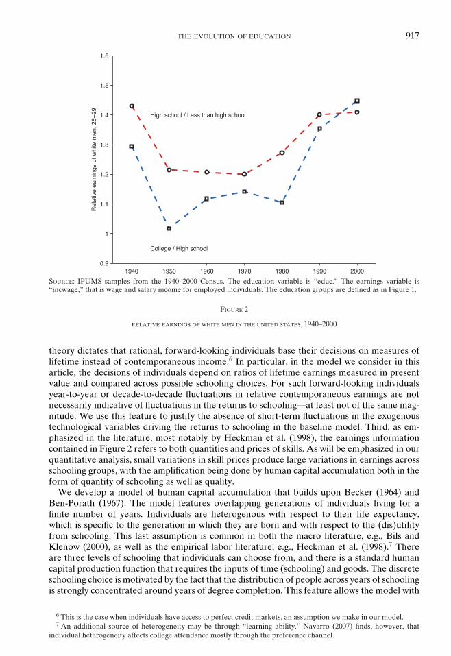
compute labor earnings of employed white males of a given cohort across three educationalgroups: less than high school, high school, and college. Figure 2 shows the corresponding relativelabor earnings between college and high school and between high school and less than highschool.

Figure 2 deserves a few comments. First, there is a noticeable decrease in both measures ofrelative earnings during the 1940s, followed by an upward trend until 2000. The decline duringthe 1940s has been documented elsewhere. Acemoglu (2002, figure 1) shows a similar patternfor the college premium, and Goldin and Katz (2008, figure 8.1) show a decline in the collegegraduate and high school graduate premia that started as early as 1915 and lasted until 1950.Kaboski (2009, figure 1) reports that the Mincerian returns to schooling exhibit the same patternas our measure of relative earnings. In addition, other measures of inequality show a U-shapeover the course of the 21st century. For instance, the share of income received by the top 1% (5and 10) of the income distribution was 16% (30 and 40) in 1919. It declined to 11% (23 and 33)in 1949 and increased to 15% (30 and 41) in 1998.5 Finally, Kopczuk et al. (2010, figure 1) showthat the Gini coefficient for earnings of workers, gathered from Social Security data since 1937,exhibits a U-shape too. Second, Figure 2 shows relative contemporaneous earnings, which pro-vide relevant information, but are only indirect measures of the returns to schooling. Economic

5 See the Historical Statistics of the United States, Millennial Edition, series Be27-29.

THE EVOLUTION OF EDUCATION 917

SOURCE: IPUMS samples from the 1940–2000 Census. The education variable is “educ.” The earnings variable is“incwage,” that is wage and salary income for employed individuals. The education groups are defined as in Figure 1.

FIGURE 2

RELATIVE EARNINGS OF WHITE MEN IN THE UNITED STATES, 1940–2000

theory dictates that rational, forward-looking individuals base their decisions on measures oflifetime instead of contemporaneous income.6 In particular, in the model we consider in thisarticle, the decisions of individuals depend on ratios of lifetime earnings measured in presentvalue and compared across possible schooling choices. For such forward-looking individualsyear-to-year or decade-to-decade fluctuations in relative contemporaneous earnings are notnecessarily indicative of fluctuations in the returns to schooling—at least not of the same mag-nitude. We use this feature to justify the absence of short-term fluctuations in the exogenoustechnological variables driving the returns to schooling in the baseline model. Third, as em-phasized in the literature, most notably by Heckman et al. (1998), the earnings informationcontained in Figure 2 refers to both quantities and prices of skills. As will be emphasized in ourquantitative analysis, small variations in skill prices produce large variations in earnings acrossschooling groups, with the amplification being done by human capital accumulation both in theform of quantity of schooling as well as quality.

We develop a model of human capital accumulation that builds upon Becker (1964) andBen-Porath (1967). The model features overlapping generations of individuals living for afinite number of years. Individuals are heterogenous with respect to their life expectancy,which is specific to the generation in which they are born and with respect to the (dis)utilityfrom schooling. This last assumption is common in both the macro literature, e.g., Bils andKlenow (2000), as well as the empirical labor literature, e.g., Heckman et al. (1998).7 Thereare three levels of schooling that individuals can choose from, and there is a standard humancapital production function that requires the inputs of time (schooling) and goods. The discreteschooling choice is motivated by the fact that the distribution of people across years of schoolingis strongly concentrated around years of degree completion. This feature allows the model with

6 This is the case when individuals have access to perfect credit markets, an assumption we make in our model.7 An additional source of heterogeneity may be through “learning ability.” Navarro (2007) finds, however, that

individual heterogeneity affects college attendance mostly through the preference channel.


three levels of schooling to capture distribution statistics such as those presented in Figure 1.At the aggregate level, the consumption good is produced with a constant-returns-to-scaletechnology requiring the input of human capital from workers of all generations and all levelsof schooling. The human capital of workers with different levels of schooling is an imperfectsubstitute in production; therefore there are three different wage rates, one for each schoollevel, clearing the labor markets. The exogenous variables are life expectancy, which increasesfrom one generation to the next, total factor productivity (TFP), and skill-biased productivityparameters in the production function.

We implement a quantitative experiment to assess the importance of changes in TFP andskill-biased productivity, as well as life expectancy, on the rise of educational attainment. Weuse data on life expectancy to discipline its model counterpart. TFP and skill-biased technicalchange are not directly observable. To discipline their paths we observe that earnings data arethe empirical counterparts of the product of human capital and wages per unit of human capital,both being endogenous objects determined in an equilibrium of our model. Thus, earnings datacan be used to discipline the paths of the neutral and skill-biased productivity variables in themodel. More generally, we choose the paths of these variables and other parameters so thatthe model’s equilibrium wages and schooling choices match a set of key statistics: educationalattainment in 1940, the trend in relative earnings across schooling levels from 1940 to 2000, andthe average growth rate of gross domestic product (GDP) per worker between 1940 and 2000.This quantitative strategy follows the approach advocated by Kydland and Prescott (1996). Inparticular, we emphasize that the parameter values are not chosen to fit the data on educationalattainment from 1940 to 2000; instead, they are chosen to mimic the trends in relative earnings,which, as mentioned earlier, provide some relevant information about the returns to schooling.

Our findings can be summarized as follows. First, our baseline experiment shows that changesin life expectancy, TFP, and skill-biased technical variables generate a substantial increase ineducational attainment. Specifically, the model implies a substantial increase in college attain-ment while underpredicting the decrease in the less than high school group and underpredictingthe increase in the high school group. In terms of the average years of schooling attained bygenerations reaching 25–29 between 1940 and 2000, the model generates an increase of 24.3%,from 10.8 years in 1940 to 13.4 in 2000, which is the same as the corresponding statistics com-puted using U.S. data. Second, we conduct a set of counterfactual experiments revealing thatthe most relevant driving variables generating the rise in educational attainment are, in or-der of importance, the “college-biased” technical variable, the “high-school-biased” technicalvariable, and life expectancy. If the college-biased technology did not rise as in our baselineexperiment, average years of schooling would increase by 14.2% instead of 24.3% in the base-line. Interestingly, if the high-school-biased technology did not rise as in the baseline, averageyears of schooling would increase faster than in the baseline (26.8%). The reason for this resultis that the lack of productivity growth at the high school level implies large returns to collegeversus high school, driving a strong increase in college attainment. When life expectancy re-mains constant, educational attainment still increases by 22.8% between 1940 and 2000 versus24.3% in the baseline. Hence, changes in life expectancy only explain about 6% of the increasein average years of schooling in the model. We show that the strong quantitative response ofschooling to skill-biased technical change is robust to other plausible forms of expectations,with a conservative scenario still accounting for 40% of the increase in average years of school-ing.8 Overall, we find that schooling responds strongly to skill-biased technical change, a resultdriven by a large change in relative earnings and not from an implausibly large elasticity ofeducational attainment. This response of schooling is informative for educational policy and forthe evaluation of related trends. For instance, the effect on educational attainment of the gapsin lifetime earnings associated with racial or gender differences or of rising costs of education.

8 As discussed earlier, we recognize the issues surrounding the reliability of the 1940 data for relative earnings, notingthe decline in relative earnings from 1940 to 1950 for both college and high school groups. However, we emphasize thatstarting the analysis in 1950 would strengthen the quantitative impact of skill-biased technical change as the impliedtrends in technology would be steeper (see Figure 2), especially so for the college group.


Our article contributes to a literature on human capital, schooling, and income inequality.9

It complements this literature by analyzing the trends in schooling in a model that remainsconsistent with the general trends in wage inequality, whereas the existing literature’s mainfocus is on explaining rising wage inequality. As discussed earlier, certain patterns of wageinequality are not as relevant for schooling decisions. To the best of our knowledge therehas been no systematic attempt to quantify and decompose the forces that lead to changesin educational attainment since 1940. Prominent papers such as Heckman et al. (1998) andGuvenen and Kuruscu (2009) focus on the determinants of rising wage inequality since the late1960s or early 1970s instead of on educational attainment itself. Lee and Wolpin (2006) andLee and Wolpin (2010) propose and estimate dynamic equilibrium models of the labor marketwith schooling and occupational choices. The main focus in these papers is on accounting forintersectoral mobility and the evolution of wages and employment structure in the UnitedStates between 1968 and 2000. Although the models have also implications for the evolutionof schooling, there is no explicit decomposition of the causes of the changes in schooling overtime.10

Our work also contributes to a literature in macroeconomics assessing the role of technicalprogress on a variety of trends.11 It also relates to the labor literature emphasizing the connec-tion between technology and education such as Goldin and Katz (2008) and the literature onwage inequality emphasizing skill-biased technical change.12 We recognize that changes in thereturns to education may not be the only explanation for rising education during this period.For instance, Glomm and Ravikumar (2001) emphasize the rise in public-sector provision ofeducation. We also recognize that educational attainment was rising well before 1940 and thatchanges in the returns to education may not be a contributing factor during the earlier period.Our focus on the period between 1940 and 2000 follows from data restrictions and the emphasisin the labor literature on rising returns to education as the likely cause of rising wage inequality.In the broader historical context, other factors may be more important such as the developmentof educational institutions and declines in schooling costs.13

The rest of the article proceeds as follows. In the next section we describe the model. InSection 3, we calibrate the model and conduct the main quantitative experiments. Section 4discusses our main results in the context of various alternative specifications and experiments.We conclude in Section 5.

2. MODEL

2.1. Environment. Time is discrete. We use t to refer to calendar time. The economy isinhabited by overlapping generations of individuals living for a finite number of periods. Thesize of each generation is normalized to one. We use τ to refer to a generation, i.e., generationτ is composed of individuals of age 1 at date t = τ. Individuals of the same generation areheterogeneous with respect to the intensity of their (dis)taste for schooling, which is representedby a ∈ R and is distributed according to the time-invariant cumulative distribution functionA.14 Individuals of different generations differ by their life expectancy, T (τ). Define A = R ×{0, 1, . . . ,∞} as the set of individual types, i.e., pairs composed of a schooling taste parameter,

9 For a review of the evidence on inequality, see Topel (1997) and Acemoglu (2002).10 He and Liu (2008) propose a model of skill accumulation to study rising wage inequality but do not explicitly model

schooling, but rather the accumulation of the stock of skills (human capital). He (2011) considers a model of discreteschooling choices with a focus on separating the contribution of demographic and technological factors in understandingthe patterns of wage inequality. Moreover, the model in He (2011), although consistent with the evolution of wageinequality, produces only a small increase in educational attainment compared to the data.

11 See Greenwood and Seshadri (2005) and the references therein.12 See, for instance, Juhn et al. (1993) and Katz and Author (1999).13 See, for instance, Goldin and Katz (2008) and Kaboski (2004).14 We abstract from ability to learn and earn across individuals as another potential source of differences in educa-

tional attainment. We recognize, however, that ability may be important for schooling choices. There are three mainmotivations for our abstraction. First, there is no complete agreement in the literature as to how ability is actually


a ∈ R, and a generation index τ ∈ {0, 1, . . . ,∞}. We assume that a and T (τ) are observed byindividuals before any decisions are made. We also assume that there is no uncertainty and thatcredit markets are perfect. We use r to denote the gross rate of interest, which is exogenouslygiven and equals the inverse of the subjective discount factor.

An individual can accumulate human capital through schooling before entering the labormarket. Let h(s, e) denote human capital once the individual starts working. It is a function ofs, the number of years spent in school, and e, which represents services affecting the qualityof education purchased by the individual while in school. Both s and e are choice variables.There are three levels of schooling labeled 1, 2, and 3. To complete level i an individual has tospend si ∈ {s1, s2, s3} periods in school and, therefore, cannot work before reaching age si + 1.We assume s1 < s2 < s3. Thus, level 1 is the model’s counterpart to the less than high schoolcategory discussed in Section 1. Similarly, level 2 corresponds to the high school category andlevel 3 to college.

There is a single consumption good produced with a constant-returns-to-scale technologyusing three inputs: the human capital of workers who completed s1 years of schooling, thehuman capital of workers who completed s2 years of schooling, and, finally, the human capitalworkers who completed s3 years. The three types of human capital are not perfect substitutesin production; thus the wage rate per unit of human capital is specific to each schooling level:wt(s) at date t.

2.2. Individuals. Preferences are defined over consumption sequences and time spent inschool. They are represented by the following utility function for an individual of type (a, τ):

τ+T (τ)−1∑t=τ

βt−τ ln (ct) − as,

where β ∈ (0, 1) is the subjective discount factor, ct is consumption during period t, and srepresents years of schooling. Note that a can be positive or negative, so that schooling provideseither a utility benefit or a cost. The distribution of a is normal with mean μ and standarddeviation σ:

A(a) = �

(a − μ

σ

),

where � is the cumulative distribution function of the standard normal distribution.The optimization problem of an individual of type (a, τ) is as follows:

maxs∈{s1,s2,s3}

{Vτ(s) − as},(1)

where Vτ(s), the lifetime utility from consumption conditional on a schooling choice, is definedby

Vτ(s) = maxe,{ct}τ+T (τ)−1

t=τ

⎡⎣τ+T (τ)−1∑

t=τ

βt−τ ln(ct)

⎤⎦ ,(2)

changing over time for the different schooling groups. Depending upon assumptions, the mapping of ability and school-ing may imply that, over time, average ability decreases, stays constant, or even increases. Second, empirical estimatesfrom structural models that have included both preference variation and ability variation seem to find that ability selec-tion is less relevant in determining schooling choices than the preference variation (see, for instance, Navarro, 2007).Third, for the type of experiment we perform in the article, namely, that we infer growth in technology to reproducepaths of earnings, changes in average ability would require different growth in technology variables, mitigating thepotential different impact on schooling over time.


subject to

τ+T (τ)−1∑t=τ

(1r

)t−τ

ct + e = h(s, e)Wτ(s),(3)

where

Wτ(s) =τ+T (τ)−1∑

t=τ+s

(1r

)t−τ

wt(s),(4)

and

h(s, e) = sηe1−η,(5)

where η ∈ (0, 1). Note that lifetime income, in the right-hand side of the intertemporal budgetconstraint (3), stipulates that labor income is earned from age s + 1 onward. Thus, this optimiza-tion program summarizes the various costs associated with acquiring education: the utility cost,the time cost, and the resource cost. We assume that s and e are chosen once and for all at thebeginning of an individual’s life. Therefore, e is the present value of educational expenditures.

Define Iτ(s), the lifetime income net of the cost of educational expenditures for an individualof generation τ conditional on schooling level s:

Iτ(s) = maxe

{h(s, e)Wτ(s) − e}.(6)

Given our assumption that the rate of interest and the subjective rate of discount are the same,i.e., βr = 1, the optimal consumption sequence is constant throughout an individual’s life andequal to Iτ(s)(1 − β)/(1 − βT (τ)). Hence,

Vτ(s) = ln(

Iτ(s)1 − β

1 − βT (τ)

)1 − βT (τ)

1 − β.

We can now turn to the characterization of an individual’s optimal choice of schooling. Notethat the value functions Vτ(s) − as are decreasing in a with slopes that are increasing (in absolutevalue) in s. Figure 3 displays these functions and describes the schooling choice of individualsfrom generation τ. Specifically, an individual of type (a, τ) chooses schooling level i over j (i > j)whenever the utility cost of schooling is low enough, that is, whenever a < aij,τ; where aij,τ isthe threshold value of a for which the individual is indifferent between i and j :

Vτ(si) − aij,τsi = Vτ(sj ) − aij,τsj .

Given the form of Vτ(s), the threshold values aij,τ are

aij,τ = 1 − βT (τ)

1 − β× 1

si − sj× ln

(Iτ(si)Iτ(sj )

).(7)

The infinite support for a ensures that each pair of value functions has a single intersectionand that there are always nonempty sets of individuals choosing the first and third level ofschooling. It is possible, however, that no individual finds it optimal to choose the second level.This situation is illustrated in Figure 3 (panel B). The schooling decision of an individual of type


aa32,τ a21,τ

Vτ (s3) − as3

Vτ (s2) − as2

Vτ (s1) − as1

A (a)

attainedcollege

attainedhigh school

attainedless than high school

Panel A – Standard case where each level of schooling is chosen by some individuals

aa31,τ

Vτ (s3) − as3

Vτ (s2) − as2

Vτ (s1) − as1

A (a)

attainedcollege

attainedless than high school

Panel B – Case where no individual chooses high school

FIGURE 3

THE DETERMINATION OF EDUCATIONAL ATTAINMENT FOR GENERATION τ


(a, τ) is therefore described as

s(a, τ) =

⎧⎪⎪⎨⎪⎪⎩

s3 if a ≤ min{a32,τ, a31,τ}s1 if a ≥ max{a21,τ, a31,τ}s2 otherwise.

(8)

In summary, the optimal choices of an individual of type (a, τ) are a schooling choice s(a, τ),an educational expenditure e(a, τ), and a consumption sequence {ct(a, τ)}τ+T (τ)−1

t=τ solving theoptimization problem (1)–(5). The specific form of the schooling choice is described in (8); theeducational expenditure is the maximizer of (6), i.e.,

e(a, τ) = s(a, τ) ((1 − η)Wτ(s(a, τ)))1/η,(9)

implying that the human capital of the individual is

h(s(a, τ), e(a, τ)) = s(a, τ) ((1 − η)Wτ(s(a, τ)))(1−η)/η ;(10)

finally, the consumption sequence satisfies

ct(a, τ) = Iτ(s(a, τ))1 − β

1 − βT (τ).

2.3. Technology. At each date, there is a single good produced with a constant returns toscale technology. We specify the production technology along the lines suggested by Goldinand Katz (2008, p. 294). That is, we assume a CES production function between college humancapital and a CES aggregate of high school and less than high school human capital:

F (H1t, H2t, H3t) = zt

((z1,tHθ

1,t + z2,tHθ2,t

)ρ/θ + z3,tHρ

3,t

)1/ρ

,

where Hi,t is the demand, at date t, for human capital supplied by individuals who completedthe ith level of schooling. The parameters ρ and θ govern the elasticity of substitution betweeninputs. Specifically, the elasticity of substitution between H1,t and H2,t is 1/(1 − θ), whereas theelasticity of substitution between H3,t and the aggregate (z1,tHθ

1,t + z2,tHθ2,t)

1/θ is 1/(1 − ρ). Theparameters zit (i = 1, 2, 3) are school-specific, exogenous productivity terms. We label the termzt as TFP, but we note that if ρ is different than θ, changes in zt are not neutral because theyaffect the marginal products of the Hi,t’s differently. Since our focus is on long-run trends, weassume constant rates of growth. Thus,

zi,t = zi,0 × gti for i = 1, 2, 3 and zt = z0 × gt,

where the gi’s are the (gross) rates of growth of the zi,ts, and the zi,0s are initial conditions.The firm’s objective is to maximize its profit:

maxH1t,H2t,H3t

F (H1t, H2t, H3t) −∑

i=1,2,3

wt(si)Hit,

implying that the following three first order conditions must hold at each date t

0 = ∂

∂HitF (H1t, H2t, H3t) − wt(si) for i = 1, 2, 3.(11)


2.4. Equilibrium. An equilibrium of the labor market involves equating the supply anddemand for human capital of individuals with schooling level i. To specify these market-clearingconditions, note that the youngest individual employed at t with s years of schooling is of age 1at date t − s; hence, this individual is from generation t − s. Thus, with a utility cost of schoolingof a, human capital of this individual at date t is h(s, e(a, t − s)). The oldest worker at date t isof age 1 at a date τ∗(t) such that τ∗ + T (τ∗) − 1 = t. Hence, the total human capital supplied atdate t by individuals having completed schooling level i is

t−si∑τ=τ∗(t)

∫h(si, e(a, τ))I{s(a, τ) = si}A(da),

where I is the indicator function. In this expression the discrete summation aggregates overgenerations working at date t whereas the integral aggregates over the taste for schoolingwithin each generation. The labor market clearing conditions are then

Hit =t−si∑

τ=τ∗(t)

∫h(si, e(a, τ))I{s(a, τ) = si}A(da) for i = 1, 2, 3.(12)

DEFINITION (1). Given r, a competitive equilibrium of the labor market is composed of (i)allocations for individuals of each type: {{ct(a, τ)}τ+T (τ)−1

t=τ , e(a, τ), s(a, τ)}(a,τ)∈A, and allocationsfor firms: {H1t, H2t, H3t}∞t=0; (ii) prices: {wt(s1), wt(s2), wt(s3)}∞t=0; such that

(1) Optimization:(i) The allocations {{ct(a, τ)}τ+T (τ)−1

t=τ , e(a, τ), s(a, τ)}(a,τ)∈A solve the optimization prob-lem of each individual (a, τ) ∈ A given prices.

(ii) The allocation {H1t, H2t, H3t}∞t=0 solves the firm’s optimization problem given prices.(2) Market clearing:

(i) Equations (12) hold at each t.

It is useful to define a notation for the educational attainment of generation τ. Let then pi,τ

be the proportion of members of generation τ having completed schooling level i:

pi,τ =∫

I{s(a, τ) = si}A(da).(13)

pi,τ is the model counterpart of the educational attainment statistics of Figure 1.15

2.5. Discussion. Equations (7) and (8) establish that the schooling decision of an individualdepends upon the semi-elasticity of net lifetime income across schooling levels. For instance,an increase in the lifetime income from college relative to high school, Iτ(s3)/Iτ(s2), raises thethreshold utility cost of entering college, a32,τ, and, therefore, increases college attainment. Themagnitude of the increase depends upon the magnitude of the change in the threshold as wellas the shape of the distribution of utility-schooling costs, A, as can be seen from Figure 3. More

15 Note that for a given level of schooling the education expenditures are constant across members of the samegeneration regardless of their taste parameter a—see Equation (9). This implies that the human capital of individualsof the same generation with the same level of schooling is also constant across individuals regardless of their taste forschooling—see Equation (10). Thus the labor market clearing condition can also be written as

Hit =t−si∑

τ=τ∗(t)

pi,τh

(si, si

((1 − η)

Wτ(si)qτ

)1/η)

for i = 1, 2, 3.


specifically, the proportion of individuals from generation τ completing college can be written,using Equation (13), as p3,τ = A(a32,τ), which implies that the evolution of college attainmentthrough time is given by

dp3,τ

dτ= A′(a32,τ)

da32,τ

dτ,(14)

and similarly, p1,τ = 1 − A(a21,τ), so that

dp1,τ

dτ= −A′(a21,τ)

da21,τ

dτ.(15)

Equations (14) and (15) deserve a few comments. First, the distribution of schooling-utilitycost, A, is relevant for the quantitative impact of changes in income on educational attainment.Given this, one concern may be our assumption that A is a Normal distribution. We have exper-imented with more flexible distributions and found that our quantitative results are essentiallyunchanged when the parameters of the distribution are calibrated as we do in Section 3.16

Second, changes in the critical values a32,τ and a21,τ are driven by changes in life expectancyand relative lifetime incomes. The relative lifetime income Iτ(si)/Iτ(sj ) for an individual ofgeneration τ contemplating school levels i and j is written, after some algebra, as

Iτ(si)Iτ(si)

= si

sj

⎛⎜⎜⎜⎜⎜⎜⎝

τ+T (τ)−1∑t=τ+si

(1r

)t−τ

wt(si)

τ+T (τ)−1∑t=τ+sj

(1r

)t−τ

wt(sj )

⎞⎟⎟⎟⎟⎟⎟⎠

1/η

.

This expression differs from one generation to the next, implying different schooling choices,because life expectancy and the future path of wages per unit of human capital differ acrossgenerations. Skill-biased technical change has a first order effect on educational attainmentbecause it can change disproportionately the wages wt(si) and wt(sj ). However, our model rulesout the possibility that skill-neutral technical change matters. To see this, imagine that wt(si)and wt(sj ) are both multiplied by the same number for each t; then the ratio Iτ(si)/Iτ(sj ) remainsconstant and educational attainment is unchanged. Whether the wt(s)’s, which are endogenous,actually behave in such a way as to generate changes in educational attainment in line with thedata is a quantitative question that we address in the next section.

3. QUANTITATIVE ANALYSIS

3.1. Calibration. The first stage of our calibration strategy is to assign values to some pa-rameters using a priori information. We let a period represent 1 year. We set the gross interestrate to r = 1.04 and the subjective discount factor to β = 1/r. For the number of years required

16 We performed these experiments using the Beta distribution for two reasons. The first is because the Beta has twoparameters, allowing us to maintain our calibration strategy. The second is because the density of the Beta distributioncan accommodate many different shapes such as uniform, bell-shaped or U-shaped and is not necessarily symmetric.Our main finding is that when we let A be a Beta distribution our calibration procedure implies parameters such thatits density is numerically very close to the normal density we calibrate in Section 3; see Restuccia and Vandenbroucke(2010).


by each level of education we use s1 = 9, s2 = 13, and s3 = 16.17 Following Bils and Klenow(2000), we choose η = 0.9.

For T (τ), the life expectancy of generation τ, we add Hazan’s (2009) measure of years spenton the market by cohort to Goldin and Katz’s (2008) figures for years of schooling achieved bycohort. We find T (1900) = 47 and T (2000) = 64 and assume a linear time trend to determinethe life expectancy of other generations.

Our specification of the production function followed Goldin and Katz (2008). These authorsprovide estimates to the required elasticity parameters. They consider three values for theelasticity of substitution between the first and second level of schooling: 2, 3, and 5. We use theintermediate value 3 so that θ = 1 − 1/3. They also consider three values for the elasticity ofsubstitution between the third level of education and the aggregate of the first two levels: 1.4,1.64, and 1.84. We use the intermediate value 1.64 so that ρ = 1 − 1/1.64.

The list of remaining parameters is

θ = (μ, σ, z1,0, z2,0, z3,0, g, g1, g2, g3) ,

which consists of the distribution parameters for the utility cost of schooling and initial levelsand growth rates for the productivity variables. We normalized the initial level of z to 1:

z0 = 1.

To assign a value to θ we build a measure of the distance between statistics generated by themodel and their empirical counterparts in the U.S. data. We target the following statistics:

1. The educational attainment of the 25–29-year-olds in the 1940 Census, that is 61% ofindividuals attaining less than high school and 31.2% of individuals attaining a highschool education. The model counterpart to these statistics is educational attainment ofthe 1921 generation, which corresponds to individuals reaching age 25 in 1940 in the U.S.data.

2. The time path of relative earnings from 1940 to 2000, displayed in Figure 2.3. The growth rate of GDP per worker from 1940 to 2000, which was on average 2%. This

target ensures that the growth rate of productivity does not imply unreasonable levels ofeconomic growth.

Even though the parameter values are chosen simultaneously to match the data targets, eachparameter has a first-order effect on some target. The levels of the technology parameters andtheir growth rates are important in matching the time path of relative earnings across schoolinggroups. The growth rate of TFP is important in matching growth in average labor productivity,but because TFP is not neutral it also matters for matching relative earnings. The distributionparameters, μ and σ, are critical in matching the distribution of educational attainment in 1940.

Formally, the calibration strategy can be described as follows. Given a value for θ we computean equilibrium trajectory and define the following objects. First,

Eij,t(θ) = wt(si)h(si, t − 25)wt(sj )h(sj , t − 25)

is the ratio of earnings between members of group i and j at the age of 25 at date t in the model.The empirical counterpart of E32,t(θ) is the relative earnings between college and high-schoolfor white males between the age of 25 and 29, denoted by E32,t. Similarly, E21,t(θ) is the model

17 Using the IPUMS samples for the 1940 and 2000 U.S. Census, we find that the average number of years spent inschool was 8.9 and 12.9 for individuals with less than high school and with high school completion. Since to solve ourmodel we need to compute discrete sums of the form given in Equation (4), we rounded these figures to s1 = 9 ands2 = 13. We assume s3 = 16 for all years.


TABLE 1CALIBRATION

Preferences β = 1/1.04, μ = 0.72, σ = 0.66Life expectancy Linear trend with T (1900) = 47 and T (2000) = 64Technology η = 0.9Productivity z0 = 1 (normalization), g = 1.012

z1,0 = 0.41, g1 = 0.996z2,0 = 0.20, g2 = 1.001z3,0 = 0.05, g3 = 1.027

counterpart of E21,t, the relative earnings between high school and less than high school. Second,we define

M(θ) =

⎡⎢⎢⎢⎣

p1,21 − 0.61

p2,21 − 0.31

Y00/Y40 − 1.0260

⎤⎥⎥⎥⎦.

Then, to assign a value to θ we solve the following minimization problem:

minθ

∑t∈T

(E32,t(θ)/E32,t − 1)2 + (E21,t(θ)/E21,t − 1)2 + M(θ)M(θ),

whereT ≡ {1940, 1950, . . . , 2000}. The first part of the objective function is the distance betweenthe relative contemporaneous earnings implied by the model and their empirical counterpart atCensus dates between 1940 and 2000. The second part of the function is the distance betweenthe model and the rest of the targets in our procedure: educational attainment in 1940 and thegrowth rate of the economy between 1940 and 2000.

At this stage it is important to describe the computational experiment leading to the deter-mination of a particular equilibrium trajectory of our model. First, observe that the decisionsof generation τ depend on the path of wages from date τ onward, as summarized in Wτ(s) inEquation (4). These wages depend on the stocks of aggregate human capital at each date which,in turn, depend on the decisions of generations prior to τ—see Equations (11) and (12). Tocircumvent this we make two assumptions. First, we assume that the economy is in a steadystate until date 0 (corresponding to 1860 in the data). That is, the first step in the determinationof an equilibrium trajectory is to determine educational attainment and human capital whenthe exogenous parameters (productivity and life expectancy) are constant at their initial values.Under this assumption we can solve for wages at any date t by assuming that the human capital,at t, of individuals born prior to date 1 is the steady-state human capital. Second, we assumethat exogenous variables start growing from date 50 (corresponding to 1910 in the data). Themotivation for this second assumption is to avoid a discontinuity in the schooling and humancapital choices between the generations up to to date 0 and date 1 and subsequent generations.Thus exogenous variables are constant from t = −∞ to t = 50 and then start growing at therate prescribed by the gi’s for productivity and as prescribed by the linear trend of T for lifeexpectancy.

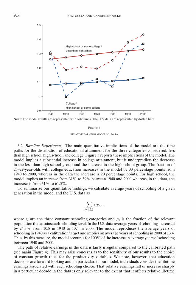
The calibrated parameters are presented in Table 1. The model is able to match well itscalibration targets. The growth rate of output per worker is 2% per year. Also, the model impliesa smooth path of relative earnings that captures the trend observed in the data as illustratedin Figure 4. In the initial steady state, 2% of a generation completed college education, 11%completed high school, and 87% attained less than high school.


1940 1950 1960 1970 1980 1990 20000.9

1

1.1

1.2

1.3

1.4

1.5

High school or some college /

Less than high school

College /

High school or some college

NOTE: The model results are represented with solid lines. The U.S. data are represented by dotted lines.

FIGURE 4

RELATIVE EARNINGS MODEL VS. DATA

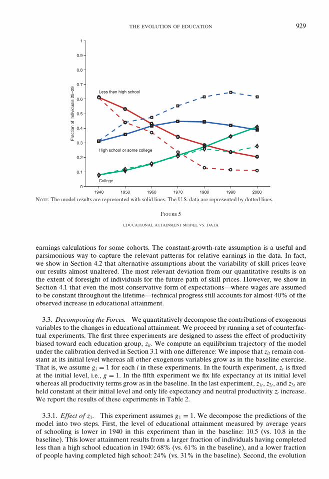
3.2. Baseline Experiment. The main quantitative implications of the model are the timepaths for the distribution of educational attainment for the three categories considered: lessthan high school, high school, and college. Figure 5 reports these implications of the model. Themodel implies a substantial increase in college attainment, but it underpredicts the decreasein the less than high school group and the increase in the high school group. The fraction of25–29-year-olds with college education increases in the model by 33 percentage points from1940 to 2000, whereas in the data the increase is 20 percentage points. For high school, themodel implies an increase from 31% to 39% between 1940 and 2000 whereas, in the data, theincrease is from 31% to 61.5%.

To summarize our quantitative findings, we calculate average years of schooling of a givengeneration in the model and the U.S. data as

∑i=1,2,3

si pi,τ,

where si are the three constant schooling categories and pi is the fraction of the relevantpopulation that attains each schooling level. In the U.S. data average years of schooling increasedby 24.3%, from 10.8 in 1940 to 13.4 in 2000. The model reproduces the average years ofschooling in 1940 as a calibration target and implies an average years of schooling in 2000 of 13.4.Thus, by this measure, the model accounts for 100% of the increase in average years of schoolingbetween 1940 and 2000.

The path of relative earnings in the data is fairly irregular compared to the calibrated path(see again Figure 4). This may raise concerns as to the sensitivity of our results to the choiceof constant growth rates for the productivity variables. We note, however, that educationdecisions are forward looking and, in particular, in our model, individuals consider the lifetimeearnings associated with each schooling choice. That relative earnings fall or increase sharplyin a particular decade in the data is only relevant to the extent that it affects relative lifetime


NOTE: The model results are represented with solid lines. The U.S. data are represented by dotted lines.

FIGURE 5

EDUCATIONAL ATTAINMENT MODEL VS. DATA

earnings calculations for some cohorts. The constant-growth-rate assumption is a useful andparsimonious way to capture the relevant patterns for relative earnings in the data. In fact,we show in Section 4.2 that alternative assumptions about the variability of skill prices leaveour results almost unaltered. The most relevant deviation from our quantitative results is onthe extent of foresight of individuals for the future path of skill prices. However, we show inSection 4.1 that even the most conservative form of expectations—where wages are assumedto be constant throughout the lifetime—technical progress still accounts for almost 40% of theobserved increase in educational attainment.

3.3. Decomposing the Forces. We quantitatively decompose the contributions of exogenousvariables to the changes in educational attainment. We proceed by running a set of counterfac-tual experiments. The first three experiments are designed to assess the effect of productivitybiased toward each education group, zit. We compute an equilibrium trajectory of the modelunder the calibration derived in Section 3.1 with one difference: We impose that zit remain con-stant at its initial level whereas all other exogenous variables grow as in the baseline exercise.That is, we assume gi = 1 for each i in these experiments. In the fourth experiment, zt is fixedat the initial level, i.e., g = 1. In the fifth experiment we fix life expectancy at its initial levelwhereas all productivity terms grow as in the baseline. In the last experiment, z1t, z2t, and z3t areheld constant at their initial level and only life expectancy and neutral productivity zt increase.We report the results of these experiments in Table 2.

3.3.1. Effect of z1. This experiment assumes g1 = 1. We decompose the predictions of themodel into two steps. First, the level of educational attainment measured by average yearsof schooling is lower in 1940 in this experiment than in the baseline: 10.5 (vs. 10.8 in thebaseline). This lower attainment results from a larger fraction of individuals having completedless than a high school education in 1940: 68% (vs. 61% in the baseline), and a lower fractionof people having completed high school: 24% (vs. 31% in the baseline). Second, the evolution


TABLE 2DECOMPOSITION

Baseline Exp. 1 Exp. 2 Exp. 3 Exp. 4 Exp. 5 Exp. 6Years of schooling

1940 10.8 10.5 10.2 10.4 10.7 11.9 9.62000 13.4 13.0 13.0 11.9 13.2 14.7 9.7% change 24.3 23.8 26.8 14.2 23.8 22.8 0.2

% change in relative earnings 2000–1940College/HS 4.46 5.09 5.45 − 2.84 3.79 9.21 − 0.74HS/Less HS 5.35 4.96 2.40 7.05 4.03 15.65 − 1.26

Annual growth ofGDP per worker (%) 2.00 2.05 1.63 1.29 1.06 2.52 0.95

NOTE: In the first experiment z1,t is kept constant at its initial level whereas all overexogenous variables are growing asin the baseline experiment. In the second experiment z2,t is constant whereas other exogenous are growing. In the thirdexperiment z3,t is constant. In the fourth zt is constant. In the fifth experiment T (τ) is constant. In the sixth experimentz1,t , z2,t , and z3,t are kept constant.

of educational attainment (from a lower initial value) is quite similar to the baseline. Averageyears of schooling increase by 23.8% between 1940 and 2000 (vs. 24.3% in the baseline). Thesmall role of growth in z1 on educational attainment is due to the fact that g1 = 0.996 in thebaseline calibration is fairly close to 1 as in this counterfactual experiment. The growth rate ofthe economy is 2.05% per year.

3.3.2. Effect of z2. This experiment assumes g2 = 1. The level of educational attainment in1940 in this experiment is lower than in the baseline and in the previous experiment: 10.2 (vs.10.8 in the baseline). This is due to a large number of individuals having completed less than highschool: 76% (vs. 61% in the baseline), and a low number of individuals having completed highschool: 16% (vs. 31% in the baseline). Through time, however, educational attainment increasesfaster in this experiment than in the baseline: average years of schooling increase by 26.8%between 1940 and 2000 (vs. 24.3% in the baseline). This increase is driven mostly by the fact thatholding z2,t constant produces an increase in the college to high school earnings ratio whereasreducing the change in the high school to less than high school earnings ratio. Specifically, in thebaseline experiment the college to high school earnings ratio increased by 4.46% between 1940and 2000 whereas in this experiment it increases by 5.45%. The high school to less than highschool earnings ratio, which increased by 5.35% in the baseline increases by only 2.40% in thisexperiment. As a result college attainment increases from 8% to 50% whereas the fraction ofindividuals with less than high school falls from 76% to 38% (vs. 61% to 20% in the baseline),driving the strong increase in average years of schooling. The growth rate of the economy is1.63% per year (vs. 2% in the baseline). This lower growth rate relative to the baseline despitea stronger increase in years of schooling is the result of lower productivity growth.

3.3.3. Effect of z3. This experiment assumes g3 = 1. The level of educational attainmentmeasured by average years of schooling in 1940 in this experiment is similar to that of the firstexperiment: 10.5 (vs. 10.8 in the baseline). The fraction of individuals having completed collegeeducation is lower than in the baseline: 2% (vs. 8% in the baseline), whereas the proportionsof those with less than high school and high school are slightly higher than in the baseline: 65%and 33% (vs. 61% and 31% in the baseline). Through time, the college to high school earningsratio decreases by 2.84% between 1940 and 2000, implying a stagnation of college attainment:2% in 2000 as in 1940. The increase in the high school to less than high school earnings ratiois 7.05%, and, as a consequence, average years of schooling increases thanks to high schoolenrollment. But the increase in average years of schooling between 1940 and 2000 is noticeablysmaller than in the baseline: 14.2% (vs. 24.3% in the baseline).

3.3.4. Effect of z. This experiment assumes g = 1. There is little effect on educational at-tainment. In 1940 average years of schooling is 10.7 (vs. 10.8 in the baseline). The difference is


due to the smaller high school and college attainment: 30% and 7% (vs. 31% and 8% in thebaseline). The evolution of educational attainment is quite similar to the baseline, with averageyears of schooling increasing by 23.8% between 1940 and 2000 (vs. 24.3% in the baseline).

3.3.5. Effect of T. When T remains constant at its initial level, educational attainment in1940 is higher than in the baseline: 11.9 years (vs. 10.8). This difference with the baseline is theresult of stronger growth in relative earnings through equilibrium effects. Unlike in the baselinemodel where increases in productivity are mitigated in equilibrium by increases in populationsize due to increasing life expectancy, in this experiment there is no offset of the productivityeffects. Through time, however, the effect of T is moderate. Between 1940 and 2000 averageyears of schooling increases by 22.8% (vs. 24.3% in the baseline). The constant populationimplies that the economy grows faster in this experiment: 2.52% (vs. 2% in the baseline).

3.3.6. Effect of z1, z2, and z3. The previous experiments suggest that T and z make a smallcontribution to the change in educational attainment over time. To assess the joint contributionof the productivity parameters biased toward various educational groups, that is z1, z2, and z3,we conduct an experiment where these three are set constant to their initial levels whereas Tand z behave as in the baseline model. First, we observe that the level of educational attainmentin 1940 is much lower than in the baseline: 9.6 years instead of 10.8. Second, the increase ineducational attainment through time is almost null since average years of schooling increase by0.2% over the 1940–2000 period (vs. 24.3% in the baseline). This is the result of the decrease inrelative earnings implied by the absence of productivity growth combined with the increase inhuman capital due to growing life expectancy.

4. DISCUSSION

4.1. Expectations. In our model, lifetime income is a critical determinant of educationalattainment and human capital accumulation as illustrated in Equations (7) and (8). One as-sumption in our quantitative assessment of skill-biased technical change in the baseline modelis that individuals have perfect foresight about the evolution of wages and hence the lifetimeincome at each schooling level. To the extent that part of the observed changes in income isdifficult to forecast, a reasonable question to ask is whether our quantitative assessment hingescritically on the perfect-foresight assumption. Hence, our aim in this section is to provide reason-able alternatives that illustrate the quantitative importance of the perfect-foresight assumption.There are in principle many alternatives to perfect foresight, but some of these have limitedapplicability in our analysis. First, in our model, individuals make once-and-for-all educationaldecisions at the beginning of their lives, taking into account the future evolution of wages andtheir impact in lifetime income in each of the educational choices. This prevents us from usingvarious forms of learning and/or adaptive expectations as alternatives to our perfect-foresightassumption. We acknowledge, however, that when schooling is modeled as a sequential choice,e.g., in each year individuals decide whether or not to stay in school for one additional year,learning and/or adaptive expectations can have an effect on the quantitative results, especiallywhen focusing on short- and medium-run episodes. Second, our focus is on long-run trends. Asa result, our analysis focuses only on alternative assumptions about the perceived path of wagesthat individuals use in comparing educational choices.

Before we describe what we do, it is important to note that individuals in our model needinformation on wages, whereas in the data, we have data on earnings that combines wages andhuman capital. The solution to our baseline model has predictions for earnings and humancapital from which we extract wage information. We use these paths for wages to constructalternative assumptions about lifetime income for individuals. More concretely, we assume thatindividuals make educational decisions from an estimate of lifetime income that is based on


TABLE 3EDUCATIONAL ATTAINMENT AND LIFETIME INCOME IN THE BASELINE MODEL WITH

PERFECT FORESIGHT AND IN THE MODEL WITH “HISTORY-BASED” EXPECTATIONS

Baseline n = 100 n = 1

Years of schooling1940 10.8 9.6 9.62000 13.4 11.5 10.5% change 24.3 20.6 9.3

% change in relative lifetime income, 1940–2000College/HS (actual) 10.6 10.6 10.6College/HS (expected) 10.6 9.8 4.6HS/Less HS (actual) 12.8 12.8 12.8HS/Less HS (expected) 12.8 15.0 7.7

past wages; we denote this estimate of lifetime income Iτ(s) given by

Iτ(s) = maxe

⎧⎨⎩h(s, e)W τ(s) − qτe : W τ(s) = wτ(s)

τ+T (τ)−1∑t=τ+s

(gs,τ,n

r

)t−τ

⎫⎬⎭ ,(16)

where gs,τ,n is a constant annual gross growth rate of wages in education level s for an individualof generation τ that is based on wages in the last n periods. Current wages across educationalcategories are observed before educational decisions are made for each generation τ. Note thatthis estimate of lifetime income differs from the lifetime income assumed in the baseline modelwith perfect foresight Iτ(s) implied by Equations (4)–(6). The estimated growth rates of wagesis a historical average over the n previous periods:

gs,τ,n =

⎧⎪⎨⎪⎩(

wτ(s)wτ−n(s)

)1/n

for n > 0

1 for n = 0.

We refer to these expectations as “history based.” Individuals make educational decisions asbefore, dictated by Equations (7) and (8), where the ratio of lifetime income Iτ(si)/Iτ(sj ) inthose equations is replaced now by the estimate Iτ(si)/Iτ(sj ) in Equation (16). In what follows,we generically refer to these ratios of lifetime income across educational categories as returnsto education.

We compute educational attainment for each generation under different specifications of nfor the history-based expectations but otherwise assuming the same parameter values as in thebaseline model. We compare the implications on educational attainment against the baselinemodel. We start by computing the case where individuals use a long historical time series ofwages to predict future income. We assume n = 100. Table 3 reports the results for averageyears of schooling in 1940 and 2000 as well as the rate of change during the period. We alsoreport the implied returns to education in each case. We emphasize that although average yearsof schooling increase at a slower pace in this experiment relative to the baseline model, thereis still a substantial increase in schooling, an increase of 20.6% between 1940 and 2000 versusthe 24.3% increase in the baseline model. We note that in this experiment average years ofschooling in 1940 is 9.6 years compared to 10.8 years in the baseline model and data. The reasonfor this discrepancy is the fact that the model is not recalibrated to the targets in the baselinemodel, and, as a result, the expected increase in lifetime income is systematically lower than the


baseline increase in lifetime income (on average expected increases in lifetime income in thisexperiment are 9% lower than in the baseline).18

For completeness, we also conduct an experiment where individuals assume that wages remainconstant throughout their lifetime, that is, we compute the case for n = 0. Table 3 reports theresults for this case. Not surprisingly, individuals underestimate the returns to schooling bothfor college and high school relative to the baseline and this has implications for the levelsof educational attainment. In this experiment, average years of schooling increase by 9.3%between 1940 and 2000 (vs. 24.3% in the baseline). Even though individuals expect wages toremain constant throughout their lifetime, each new cohort observes current relative wageswhen making educational decisions that affect their choices. This effect alone explains 38%(9.3/24.3) of the increase in average years of schooling between 1940 and 2000.19

We conclude that although the extent of foresight of future wages is important for thecontribution of skill-biased technical progress to the increase in educational attainment, in themost conservative scenario where individuals assume constant wages throughout, the impactof skill-biased technology still implies a substantial increase in educational attainment, almost40% of the observed increase in average years of schooling.

4.2. Time-Series Variability in Relative Earnings. Another potentially relevant feature in thetime series of relative earnings across schooling groups is the decade-to-decade variation (seeagain Figure 4). Although in the baseline model we captured the long-run path for these series, arelevant question is whether fluctuations in relative earnings around these trends are importantfor the overall contribution of skill-biased technological progress to the increase in schooling.To the extent that educational decisions by individuals are made based on measures of lifetimeincome, we expect that variability around the trend does not have a first-order impact on theoverall contribution of skill-biased technical progress to the increase in schooling. Nevertheless,the objective in this section is to assess the quantitative importance of the fluctuations in relativeearnings for the results.

As discussed earlier, there is not a simple decomposition of relative earnings in the databetween wages and human capital. Broadly speaking, to circumvent this issue, we feed in aseries of wages in the model such that the implied optimal human capital decisions of individualsgenerate the relative earnings we observe in the data. We emphasize two main findings. First,we find, perhaps not so surprisingly, that we need small deviations in trend growth for wagesto capture the fluctuations in relative earnings seen in the data. Second, educational attainmentimplied by the model is fairly close to the baseline. For instance, in 1940, 63% of individualsattained less than high school (vs. 61% in the baseline) and 28% attained high school (vs. 31%in the baseline), implying 10.75 years of schooling in 1940 (vs. 10.8 in the baseline). The modelalso implies an increase in average years of schooling between 1940 and 2000 of 25.5% (vs.24.3% in the baseline).

We conduct the same experiments related to the perfect-foresight assumption as in theprevious section to assess the impact of fluctuations in relative earnings. In the long history casewhere n = 100, that is when individuals use a long time series of data to evaluate the growth rateof wages, educational attainment measured by average years of schooling increases by 20.5%(vs. 20.6% with trend wages and 24.3% in the baseline). When individuals expect no changes in

18 To the extent that the level of educational attainment is useful in pinning down the elasticity of schooling onincome changes, as discussed previously, we find it of interest to also evaluate the implications of the same experimentbut with a recalibration of the distribution of schooling costs (μ and σ) to match the average years of schooling in 1940in the data. We note that the ratio of lifetime income in the model is independent of μ and σ, and, as a result, theimplications on lifetime income in this experiment are the same as in the model without the recalibration. We find inthis case that the experiment generates an increase in average years of schooling of 23.3%, which is larger than the onewithout recalibration and closer to the baseline experiment.

19 When adjusting the parameters of the cost-of-schooling distribution to match the average years of schooling in1940, this experiment produces an increase in average years of schooling of 12.6% compared to the 9.3% withoutrecalibrating and 24.3% in the baseline.


relative earnings, the case where n = 0, average years of schooling increases by 9% (vs. 9.3%with trend wages).

We conclude that although decade-by-decade fluctuations in relative earnings may be poten-tially important for educational decisions, these fluctuations are not quantitatively importantin reducing the overall contribution of skill-biased technical change on schooling in the perfectforesight case as well as the more conservative type of expected income.

4.3. Other Items. The model delivers an elasticity of educational attainment to changes inlifetime income that is driven mostly by skill-biased technical change. As argued previously,a critical aspect of the discipline of this elasticity in our calibration is from the utility cost ofschooling to match the distribution of educational attainment. We discuss the reasonablenessof the implied elasticity by looking at closely related empirical and model-based evidence. Wealso connect the implications of the implied elasticity for educational policy and other trendsthat may affect relative incomes. Next, we discuss the relevance for our results of consideringhuman capital accumulation on the job.

4.3.1. The elasticity of educational attainment. There is a large empirical literature assessingthe impact of educational policy on schooling. The typical focus is on assessing the responseof college attainment to changes in subsidies or other factors that alter lifetime incomes suchas Dynarski (2002, 2003), van der Klaauw (2002), and Keane and Wolpin (1997). Althoughthere is no complete agreement on the exact magnitude of these elasticities, the evidencesuggests that they are large, and we use this evidence to provide a benchmark against which toassess the magnitude implied by our quantitative results. For instance, Keane and Wolpin (1997)estimate a life-cycle model of schooling and career choices. Their structural estimates imply thatsubsidizing college costs by about 50% increases college completion from 28.3% to 36.7%. Toconstruct an elasticity, we calculate that the subsidy represents about 1% of lifetime income.20

This implies an elasticity of college completion of ln(36.7/28.3)/ln(1.01) = 26. We calculate thatin our model a subsidy of the same size, that is 1% of the lifetime income from college for the 1981generation (the generation whose educational attainment is measured in 2000) yields an increasein college attainment from 40.8 to 45.5, that is, an elasticity of ln(45.5/40.8)/log(1.01) = 11.

Dynarski (2003) studies an exogenous change in education policy—namely, the elimination ofthe Social Security Student Benefit program in the United States in 1981—that affected somestudents but not others. Dynarski found that $1,000 (dollars of year 2000) in college subsidygenerates an increase in college enrollment of 3.6 percentage points. We can also relate to thisfinding by performing the same policy experiment. To obtain an increase in college enrollmentof 3.6 percentage points in 2000 in the model, a subsidy to college equivalent to 0.8% oflifetime income is needed, which, we argue, is a larger number than $1,000. We concludefrom these experiments that the strong effect of skill-biased technical change on educationalattainment in the baseline model comes from strong changes in relative earnings and not froman implausibly large elasticity of educational attainment. The quantitative magnitude of theresponse of schooling to changes in relative lifetime income is relevant for educational policyand for the impact evaluation of other related trends. For example, it is often viewed that theracial gap in schooling is related primarily to underinvestments in education in the early part oflife. Our results suggest that another important factor is the gap in lifetime earnings associatedwith racial differences. Similarly, there have been recent discussions on the rising costs of collegein explaining a recent slowdown in college enrolment. In the context of our model, rising costs ofeducation can have implications for schooling to the extent that they affect the relative lifetimeearnings (net of educational costs).

20 Keane and Wolpin’s (1997) subsidy is $2,000 per year for four years. The present value of a $35,000 annual incomefor 40 years, discounted at 4%, is about $730,000. So, we found 2000 × 4/730,000 = 0.01.


4.3.2. Experience. Our model abstracts from human capital accumulated on the job. Thedata suggest that there are considerable returns to experience. The age profile of earnings, forexample, is increasing in the data, whereas our baseline model implies that they are decreasing.Returns to experience may affect educational decisions. First, if they increase with education—as has been documented is the case in the data—then this provides an additional return toschooling, reinforcing the effects of skill-biased technical change. Second, substantial returns toexperience imply that, other things being equal, individuals would have an incentive to enter thelabor market sooner. Because of these opposing effects, it is a quantitative question whetheron-the-job human capital accumulation affects the evolution of educational attainment overtime. We have experimented adding on-the-job human capital accumulation to the model andfound that under a reasonable calibration of the returns to experience, our baseline resultsremain after adding experience.21

5. CONCLUSION

We developed a model of human capital accumulation to address the role of changes in thereturns to education on the rise of educational attainment in the United States between 1940and 2000. The model features discrete schooling choices and individual heterogeneity so thatpeople sort themselves into the different schooling groups. In the model, skill-biased technicalchange increases the returns to schooling, thereby creating an incentive for more people toattain higher levels of schooling. We find that changes in the returns to education generate asubstantial increase in educational attainment and that this quantitative importance is robust torelevant variations in the model. We also found that the substantial changes in life expectancyin the data turn out to explain a small portion of the change in educational attainment in themodel.

There are several issues that would be worth exploring further. First, we have not addressedthe factors that may contribute to the slowdown in college attainment since the late 1970s. As-sessing the contribution of rising college costs together with tighter borrowing constraints maybe important. Second, it would be interesting to assess the role of changes in the returns to edu-cation on educational attainment in other contexts such as across genders, races, and countries.For instance, it would be relevant to investigate changes in the returns to schooling in countrieswith different labor-market institutions. Institutions that compress wages may reduce the in-centives for schooling investment and, perhaps, holding other institutional aspects constant, thiswage compression may explain the lower educational attainment in some European countriescompared to the United States. Similarly, it is relevant to explore the changes in the returns toeducation for women in conjunction with the observed increase in labor market participationand the reduction in the gender wage gap. A glance at the data suggests that changes in thereturns to schooling for women have been similar to that of men. Hence, together with fasteroverall wage growth and an increase in labor market hours for women may explain the largerincrease in educational attainment observed for women between 1940 and 2000. Third, ouranalysis has taken the direction of technical change as given. It would be interesting to studyquantitatively the process of human capital accumulation allowing for endogenous technicalchange in the spirit of Galor and Moav (2000). We leave all these relevant explorations forfuture research.

REFERENCES

ACEMOGLU, D., “Technical Change, Inequality, and the Labor Market,” Journal of Economic Literature40 (2002), 7–72.

BECKER, G., Human Capital: A Theoretical and Empirical Analysis with Special Reference to Education(Chicago: The University of Chicago Press, 1964).

21 For more details on these experiments see Restuccia and Vandenbroucke (2010).


BEN-PORATH, Y., “The Production of Human Capital and the Life-Cycle of Earnings,” Journal of PoliticalEconomy 75 (1967), 352–65.

BILS, M., AND P. J. KLENOW, “Does Schooling Cause Growth?”American Economic Review 90 (2000),1160–83.

DYNARSKI, S., “The Behavioral and Distributional Implications of Aid for College,” American EconomicReview 92 (2002), 279–85.

———, “Does Aid Matter? Measuring the Effect of Student Aid on College Attendance and Completion,”American Economic Review 93 (2003), 279–88.

GALOR, O., AND O. MOAV, “Ability-Biased Technological Transition, Wage Inequality, and EconomicGrowth,” Quarterly Journal of Economics 115 (2000), 469–97.

GLOMM, G., AND B. RAVIKUMAR, “Human Capital Accumulation and Endogenous Public Expenditures,”Canadian Journal of Economics 34 (2001), 807–26.

GOLDIN, C., AND L. KATZ, The Race between Education and Technology (Cambridge, MA: The BelknapPress of Harvard University Press, 2008).

GREENWOOD, J., AND A. SESHADRI, “Technological Progress and Economic Transformation,” in P. Aghionand S. N. Durlauf, eds., Handbook of Economic Growth (Amsterdam: Elsevier, 2005), 1225–73.

GUVENEN, F., AND B. KURUSCU, “A Quantitative Analysis of the Evolution of the U.S. Wage Distribution:1970–2000,” in D. Acemoglu, K. Rogoff and M. Woodford, eds., NBER Macroeconomics Annual(Chicago: The University of Chicago Press, 2009), 227–76.

HAZAN, M., “Longevity and Lifetime Labor Supply: Evidence and Implications,” Econometrica 77 (2009),1829–63.

HE, H., “What Drives the Skill Premium: Technological Change or Demographic Variation?” Workingpaper, University of Hawaii, 2011.

———, AND Z. LIU, “Investment-Specific Technological Change, Skill Accumulation, and Wage Inequal-ity,” Review of Economic Dynamics 11 (2008), 314–34.

HECKMAN, J. J., L. LOCHNER, AND C. TABER, “Explaining Rising Wage Inequality: Explorations with aDynamic General Equilibrium Model of Labor Earnings with Heterogeneous Agents,” Review ofEconomic Dynamics 1 (1998), 1–58.

———, L. J. LOCHNER, AND P. E. TODD, “Fifty Years of Mincer Earnings Regressions,” NBER WorkingPaper No. 9732.

JUHN, C., K. MURPHY, AND B. PIERCE, “Wage Inequality and the Rise in Returns to Skill,” Journal ofPolitical Economy 101 (1993), 410–42.

KABOSKI, J., “Supply Factors and the Mid-Century Fall in the Skill Premium,” Working Paper, Ohio StateUniversity, 2004.

———, “Education, Sectoral Composition, and Growth,” Review of Economic Dynamics 12 (2009), 168–82.

KATZ, L., AND D. AUTHOR, “Changes in the Wage Structure and Earnings Inequality” in O. Ashenfelterand D. Card, eds., Handbook of Labor Economics (Amsterdam: Elsevier, 1999), 1463–555.

KEANE, M., AND K. WOLPIN, “The Career Decisions of Young Men,” Journal of Political Economy 105(1997), 473–522.

KOPCZUK, W., E. SAEZ, AND J. SONG, “Earnings Inequality and Mobility in the United States: Evidencefrom Social Security Data since 1937,” The Quarterly Journal of Economics 125 (2010), 91–128.

KYDLAND, F. E., AND E. C. PRESCOTT, “The Computational Experiment: An Econometric Tool,” TheJournal of Economic Perspectives 10 (1996), 69–85.

LEE, D., AND K. WOLPIN, “Intersectoral Labor Mobility and the Growth of the Service Sector,” Economet-rica 74 (2006), 1–46.

———, AND ———, “Accounting for Wage and Employment Changes in the US from 1968–2000: ADynamic Model of Labor Market Equilibrium,” Journal of Econometrics 156 (2010), 68–85.

NAVARRO, S., “Using Observed Choices to Infer Agent’s Information: Reconsidering the Importanceof Borrowing Constraints, Uncertainty and Preferences in College Attendance,” Working paper,University of Wisconsin, Madison, 2007.

———, AND C. URRUTIA, “Intergenerational Persistence of Earnings: The Role of Early and CollegeEducation,” American Economic Review 94 (2004), 1354–78.

RESTUCCIA, D., AND G. VANDENBROUCKE, “The Evolution of Education: A Macroeconomic Analysis,”Working Paper 388, Department of Economics, University of Toronto, 2010.

TOPEL, R., “Factor Proportions and Relative Wages: The Supply-Side Determinants of Wage Inequality,”The Journal of Economic Perspectives 11 (1997), 55–74.

VAN DER KLAAUW, W., “Estimating the Effect of Financial Aid Offers on College Enrollment: ARegression-Discontinuity Approach,” International Economic Review 43 (2002), 1249–87.

Date post:	13-Feb-2017
Category:	Documents
Upload:	dodang
View:	223 times
Download:	1 times

THE EVOLUTION OF EDUCATION: A MACROECONOMIC ANALYSIS

Documents