THE EXPLICIT SOLUTIONS OF LINEAR LEFT-INVARIANT SECOND ORDER STOCHASTIC EVOLUTION EQUATIONS ON THE 2D-EUCLIDEAN MOTION GROUP REMCO DUITS AND MARKUS VAN ALMSICK Abstract. We provide the solutions of linear, left-invariant, 2nd-order sto- chastic evolution equations on the 2D-Euclidean motion group. These solu- tions are given by group-convolution with the corresponding Green’s functions that we derive in explicit form in Fourier space. A particular case coincides with the hitherto unsolved forward Kolmogorov equation of the so-called di- rection process, the exact solution of which is required in the field of image analysis for modeling the propagation of lines and contours. By approximating the left-invariant base elements of the generators by left-invariant generators of a Heisenberg-type group, we derive simple, analytic approximations of the Green’s functions. We provide the explicit connection and a comparison be- tween these approximations and the exact solutions. Finally, we explain the connection between the exact solutions and previous numerical implementa- tions, which we generalize to cope with all linear, left-invariant, 2nd-order stochastic evolution equations. 1. Introduction Pixel-independent image analysis usually starts with the sampling of an image f ∈ L 2 (R 2 ) by a function ψ ∈ L 2 (R 2 ) via f → (ψ,f ) L2(R 2 ) . To probe an image at every location x ∈ R 2 and in every direction e iθ ∈ T one translates and rotates an anisotropic test function by means of a representation g →U g of the Euclidean motion group U g ψ(y)= ψ(R -1 θ (y - x)), g =(x,e iθ ). The result of such an image sampling is a function U f ∈ L 2 (G) on the Euclidean motion group manifold G = R 2 T, which is given by U f (g)=(U g ψ,f ). Throughout this article we refer to function U f as the orientation score of image f . The generation of orientation scores and the reconstruction of images thereof has been the subject of previous publications. The subsequent section 2 will provide a brief overview and an embedding in wavelet theory. For the remainder of the article we assume the orientation score as given and focus on operations on U f that are inspired by stochastic processes modeling the propagation of lines and contours. As a class of left invariant operators we consider in section 3 all linear, second order, left-invariant evolution equations and their resolvents on L 2 (R 2 T), which correspond to Forward Kolmogorov equations of left-invariant stochastic processes on the Euclidean motion group. Date : March 28, 2006 and, in revised form ?? 2000 Mathematics Subject Classification. Primary 22E25, 37L05, 68U10 ; Secondary 34B30, 47D06 . Key words and phrases. Lie Groups, Stochastic Evolution Equations, Image Analysis, Direc- tion Process, Completion Field. The Netherlands Organization for Scientific Research is gratefully acknowledged for financial support. 1
Transcript
THE EXPLICIT SOLUTIONS OF LINEAR LEFT-INVARIANTSECOND ORDER STOCHASTIC EVOLUTION EQUATIONS ON
THE 2D-EUCLIDEAN MOTION GROUP
REMCO DUITS AND MARKUS VAN ALMSICK
Abstract. We provide the solutions of linear, left-invariant, 2nd-order sto-chastic evolution equations on the 2D-Euclidean motion group. These solu-
tions are given by group-convolution with the corresponding Green’s functions
that we derive in explicit form in Fourier space. A particular case coincideswith the hitherto unsolved forward Kolmogorov equation of the so-called di-
rection process, the exact solution of which is required in the field of image
analysis for modeling the propagation of lines and contours. By approximatingthe left-invariant base elements of the generators by left-invariant generators
of a Heisenberg-type group, we derive simple, analytic approximations of the
Green’s functions. We provide the explicit connection and a comparison be-tween these approximations and the exact solutions. Finally, we explain the
connection between the exact solutions and previous numerical implementa-tions, which we generalize to cope with all linear, left-invariant, 2nd-order
stochastic evolution equations.
1. Introduction
Pixel-independent image analysis usually starts with the sampling of an imagef ∈ L2(R2) by a function ψ ∈ L2(R2) via f 7→ (ψ, f)L2(R2). To probe an imageat every location x ∈ R2 and in every direction eiθ ∈ T one translates and rotatesan anisotropic test function by means of a representation g 7→ Ug of the Euclideanmotion group Ugψ(y) = ψ(R−1
θ (y − x)), g = (x, eiθ). The result of such an imagesampling is a function Uf ∈ L2(G) on the Euclidean motion group manifold G =R2 o T, which is given by Uf (g) = (Ugψ, f). Throughout this article we refer tofunction Uf as the orientation score of image f .
The generation of orientation scores and the reconstruction of images thereof hasbeen the subject of previous publications. The subsequent section 2 will provide abrief overview and an embedding in wavelet theory. For the remainder of the articlewe assume the orientation score as given and focus on operations on Uf that areinspired by stochastic processes modeling the propagation of lines and contours.As a class of left invariant operators we consider in section 3 all linear, secondorder, left-invariant evolution equations and their resolvents on L2(R2 o T), whichcorrespond to Forward Kolmogorov equations of left-invariant stochastic processeson the Euclidean motion group.
Date: March 28, 2006 and, in revised form ??2000 Mathematics Subject Classification. Primary 22E25, 37L05, 68U10 ; Secondary 34B30,
47D06 .Key words and phrases. Lie Groups, Stochastic Evolution Equations, Image Analysis, Direc-
tion Process, Completion Field.The Netherlands Organization for Scientific Research is gratefully acknowledged for financial
support.
1
2 REMCO DUITS AND MARKUS VAN ALMSICK
First we show that the solutions of these partial differential equations are givenby a convolution with the corresponding Green’s function. Then we provide explicitformulas for these Green’s functions. To cope with the cyclic boundary conditionsin θ we follow two separate approaches. In the first approach, we expand theGreen’s kernel in series of Mathieu functions as described in the literature aboutthe Mathieu equation [31]. The resulting series of Mathieu functions convergesonly slowly for group elements near the unity element, but we utilize this solutionfor a generalization of a numerical algorithm of direction process by August [3]and derive a new and exact computation scheme1. In the second approach, weunwrap the torus T in θ and solve the partial differential equations for absorbingθ-boundaries at infinity to eventually map the solution back onto the torus T.Adding all mapped branches of the solution renders the Green’s function for cyclicboundaries as a sum of rapidly decaying terms. Both approaches are describedfor the special case of the direction process in section 4 and for all other cases insection 5.
In section 4.3 we approximate the left invariant base elements of the Euclideangroup generators by left-invariant generators of a Heisenberg-type group. The re-sulting equations render simple, analytic approximations of the exact Green’s func-tions and provide explicit and simple formulas for the modes of so-called completionfields, which are the probability distributions of stochastic processes on R2 oT withgiven source and given sink.
The numeric algorithm that solves all linear, left-invariant, 2nd-order stochasticevolution equations on a discrete grid in Fourier space and its relation to our firstanalytic approach is the subject of the last section 6.
2. Orientation Scores
In many image analysis applications an object Uf ∈ L2(G) defined on the 2D-Euclidean motion group G = R2 o T is constructed from a 2D-grey-value imagef ∈ L2(R2). Such an object provides an overview of all local orientations in animage. This is important for image analysis and perceptual organization, [27], [19],[30], [15], [13], [41], [34], [4] and is inspired by our own visual system, in whichreceptive fields exist that are tuned to various locations and orientations, [37], [6].In addition to the approach given in the introduction other schemes to constructUf : R2 o T → C from an image f : R2 → R exist, but only few methods putemphasis on the stability of the inverse transformation Uf 7→ f .
In this paragraph we provide an example on how to obtain such an object Uffrom an image f . This leads to the concept of invertible orientation scores, which wedeveloped in previous work, [9], [13], [11], and which we briefly explain here. An ori-entation score Uf : R2 o T → C of an image f : R2 → R is obtained by means of ananisotropic convolution kernel ψ : R2 → C via Uf (g) =
∫R2 ψ(R−1
θ (x− y))f(y) dy,g = (x, eiθ) ∈ G = R2 o T, Rθ ∈ SO(2). This differs from standard contin-uous wavelet theory, see for example [28] and [2], where the wavelet transformis constructed by means of a quasi-regular representation of the similitude groupRd o T× R+, which is unitary, irreducible and square integrable (admitting the ap-plication of the more general results in [21]), in the sense that we do allow a stablereconstruction already at a single scale orientation score for a proper choice of ψ. In
1We provide the complete bi-orthogonal base of eigenvectors of the matrix in this linearalgorithm.
LINEAR LEFT-INVARIANT EVOLUTIONS ON THE 2D-EUCLIDEAN MOTION GROUP 3
standard wavelet reconstruction schemes it is not possible to obtain an image f in awell-posed manner from a “fixed scale layer”, that is fromWψf(·, ·, σ) ∈ L2(R2oT),for fixed σ > 0.2 The general wavelet reconstruction results [21] do not apply tothe transform f 7→ Uf , since the left regular representation of the Euclidean mo-tion group on L2(R2) is reducible. In earlier work we therefore provided a generaltheory [9], [7], [8], to construct wavelet transforms associated with admissible vec-tors/ distributions.3 With these wavelet transforms we construct orientation scoresUf : R2 o T → C by means of admissible line detecting vectors4 ψ ∈ L2(R2) suchthat these transforms are unitary in a reproducing kernel Hilbert space CGK , whichis a closed subspace of L2(G).
With this well-posed, unitary transformation between the space of images andthe space of orientation scores at hand, we can perform image processing via orien-tation scores, see [11], [13], [27]. For the remainder of the article we assume that theobject Uf is some given function in L2(R2 oT) and we write U ∈ L2(R2 oT) ratherthan Uf ∈ CGK . For all image analysis applications where an object Uf ∈ L2(R2oT)is constructed from an image f ∈ L2(R2), operators on the object U ∈ L2(R2 o T)must be left invariant to ensure Euclidean invariant image processing [9]p.153. Thisapplies also to the cases where the original image cannot be reconstructed in a stablemanner as in channel representations [18] and steerable tensorvoting [20].
3. Left Invariant Evolution Equations on the Euclidean MotionGroup
In order to construct the left invariant evolution equations on the EuclideanMotion group and to understand their structure we first compute the left invariantvector fields and their commutators on the Euclidean motion group. This struc-ture has more or less been overlooked in previous work on the forward Kolmogorovequation of the well-known direction process, [32], [36], [42] and [3]. This struc-ture will be relevant for our derivation of the solution of this evolution equation.Moreover, it provides a full overview on linear second order left invariant evolutionequations on the Euclidean motion group and thereby it provides more general andalternative left invariant stochastic processes on the Euclidean motion group.
Let G = R2 o T be the Euclidean Motion group with group product
g g′ = (x, eiθ)(x′, eiθ′) = (x +Rθx′, ei(θ+θ
′)) , g = (x, eiθ), g′ = (x′, eiθ′) ∈ R2 o T,
with unity element e = (0, 1) and Rθ =(
cos θ − sin θsin θ cos θ
). Let ex, ey be a
positively oriented orthonormal base in R2. Let eθ be a unit tangent vector at theunit element of T. Then the tangent space at the unity element Te(G) is spannedby
(3.1) Te(G) = A1, A2, A3 := eθ, ex, ey.
2The same problem arises in linear scale space theory where it is impossible to reconstruct theoriginal image in a stable L2-preserving matter from a fixed scale restriction uα
f (·, s) of a scale
space representation uαf : Rd × R+ → R obtained by an evolution equation on Rd generated by
−(−∆)α, 0 < α ≤ 1, [12].3Depending whether images are assumed to be band-limited or not, for details see [8].4Or rather admissible distributions ψ ∈ H−(1+ε),2(R2), ε > 0 if one does not want a restriction
to bandlimited images.
4 REMCO DUITS AND MARKUS VAN ALMSICK
As we will see this basis yields the following left invariant vector fields on G,eθ, eξ, eη which are defined by
(3.2)eθ(x, eiθ) = eθ,eξ(x, eiθ) = cos θ ex + sin θ ey ,eη(x, eiθ) = − sin θ ex + cos θ ey ,
where we identified Tg=(x,eiθ)(R2, eiθ) with Te(R2, ei0) and Tg=(x,eiθ)(x,T) withTe(0,T), by means of parallel transport (on R2 respectively T). The tangent spaceTe(G) is a 3D Lie algebra equipped with Lie product
[A,B] = limt↓0
a(t)b(t)(a(t))−1(b(t))−1 − e
t2,
where t 7→ a(t) resp. t 7→ b(t) are any smooth curves in G with a(0) = b(0) = eand a′(0) = A and b′(0) = B. The Lie products of the base elements in (3.1) are
[A1, A2] = A3, [A1, A3] = −A2, [A2, A3] = 0 .
The left respectively right regular representations of G onto L2(G) are given byL : G → B(L2(G)) : g 7→ Lg and R : G → B(L2(G)) : g 7→ Rg, where Lg andRg are given by LgΦ(h) = Φ(g−1h) and RgΦ(h) = Φ(hg), for all g, h ∈ G andΦ ∈ L2(G). An operator Φ on L2(G) is called left invariant if it commutes with theleft-regular representation, that is ΦLg = Lg Φ for all g ∈ G. A vector field (nowconsidered as differential operators) A on G is called left invariant if it satisfies
Agφ = Ae(φ Lg) = Ae(h 7→ φ(g h)) ,
for all infinitely differentiable functions φ ∈ C∞c (Ωg) where Ωg is an open set around
g within G and with the left multiplication Lg : G→ G given by Lg(h) = g h.Recall that the linear space of left-invariant vector fields L(G) equipped with the
Lie product [A, B] = AB−BA is isomorphic to Te(G) by means of the isomorphism
In this article we will derive exact analytic solutions and close analytic approxima-tions which are much more tangible/easier to compute of the following 2nd orderlinear left invariant evolution equations
(3.4)
∂t℘ = A ℘ ,limt↓0
℘(·, t) = U(·) , in L2(R2 o T).
LINEAR LEFT-INVARIANT EVOLUTIONS ON THE 2D-EUCLIDEAN MOTION GROUP 5
where the negative definite generator A acting on L2(G) is given by
(3.5) A = −3∑i=1
aiAi +3∑
i,j=1
DijAiAj ai, Dij ∈ R, i = 1, . . . , 3.
where we are only interested in the case where the constant matrix D is a semi-positive diagonal matrix, i.e. Dij = Diiδij , with Dii ≥ 0, i = 1, . . . 3 in which casethe generator becomes
(3.6) A =[−a1∂θ − a2∂ξ − a3∂η +D11(∂θ)2 +D22(∂ξ)2 +D33(∂η)2
].
The first order part of the generator takes care of transport (convection) and thesecond order part takes care of diffusion in the Euclidean motion group G. Notethat the non-commutative nature of the Euclidean motion group, recall (3.3) makesthese evolution equations complicated. Furthermore we note that these evolutionequations are indeed left invariant as their generator is left-invariant (since it isconstructed by linear combinations of products of left invariant vector fields).
The motivation for considering these left invariant evolution equation comes fromprobability theory. Consider the following stochastic equation on R2 o T
with ξ = (ξ1, ξ2, ξ3), where the components are independent random variables ξi
which are Gaussian white noise distributed. The solution of which is given by
(3.8) g(t) = g0 +∫ t
0
a(g(s), s)ds +∫ t
0
B(g(s), s)ξ(s)ds.
For the exact meaning of the Stochastic differential equation (3.7) and the corre-sponding stochastic integral (3.8) and further details on stochastic processes see[33]. In this article we shall only consider the case where B(g(s), s) and a(g(s), s)are left invariant and not explicitly dependent on s. In this case it does not matterwhether one uses Stranovitch or Ito calculus for the stochastic integrals and byIto’s formula for functions on the process t 7→ (t, g(t)) we obtain the following leftinvariant evolution equation for the transition densities
(3.9) ∂tp(g, t |g0, t0) = −∑i=1
Aiaip(g, t|g0, t0) +12
3∑i,j=1
AiAj [BBT ]ijp(g, t|g0, t0)
which is known as the Forward Kolmogorov equation of the stochastic process givenby (3.7). In equation (3.9) we omitted the dependence of ai and Bij on g becausewe have shown that to ensure left-invariance of the generator the components ofa and B with respect to the basis Ai3i=1 must be constant, [38]. The ForwardKolmogorov equations of left invariant stochastic processes (with constant a, B,D = 1
2BTB) are given by (3.4) and (3.5). These transition densities (3.9) are to be
considered as limiting distributions of conditional probability densities of discreteprocesses (random walks) on the Euclidean motion group. Consider for examplethe special case of the well-known direction process [32], [4], [41] where a randomwalker moves in the spatial plane along its current direction in the spatial plane(that is along ξ = x cos θ+ y sin θ) and where the average curvature of its path5 is
5That is κ = 1L
R L0 k(s) ds = 1
L
R L0 |θ(s)| ds ∼ N (0, σ2), which explains the N in (3.10).
6 REMCO DUITS AND MARKUS VAN ALMSICK
Gaussian distributed with variance σ2 = 2D11
(3.10)
eiθ(sk+∆s) = ei(θ(sk)+∆s η), Var(η) = N σ2
x(sk + ∆s) = x(sk) + ∆s(
cos θ(sk)sin θ(sk)
)∆s = L
N , with L ∼ NE(α), k = 0, . . . , N − 1.
The corresponding forward Kolmogorov equation is a special case (namely puta1 = a3 = D22 = D33 = 0) of (3.4) and (3.5).
In Section 4 we shall consider these evolution equations and provide the exactanalytic solutions (and even more tangible analytic approximations) of both theevolution equations and their resolvent equations, which were strongly required(but not yet found) in the fields of applied mathematics and image analysis.
In Section 5 we also derive explicit solutions for other cases such as D22 =D33 = D11 = 0 (convection without diffusion), a1 = a3 = 0 and D22 = D33 > 0 (aforward-Kolomogorov equation of a direction process including isotropic diffusion inthe plane), and the case a1 = a2 = a3 = 0, Dii > 0, i = 1, 2, 3 (only diffusion). Fur-thermore in Section 6 we discuss an efficient method to compute the exact Green’sfunctions in all cases (with periodic boundary conditions), where we explicitly putthe connection with the exact solutions (with periodic boundary conditions) in thespecial cases above. We also point to Appendix A where we use Fourier transformon the Euclidean motion group R2 o T rather than Fourier transform on R2 toobtain alternative (but analogue) formulas for the solutions.
In Sections 4 & 5 we shall use the following conventions:
• The unit-step function u : R → R is given by u(x) = 1 if x > 0 and u(x) = 0if x < 0 and u(0) = 1
2 .• Fourier transform F : L2(R2) → L2(R2), is almost everywhere defined by
[F(f)](ω) = f(ω) =1
(2π)
∫R2f(x) e−iω·x dx .
We use the following notation for Euclidean/polar coordinates in spatial andFourier domain, respectively: x = (x, y) = (r cosφ, r sinφ), ω = (ωx, ωy) =(ρ cosϕ, ρ sinϕ), with φ, ϕ ∈ [0, 2π), r, ρ>0.
• Let G = R2 o T be the Euclidean motion group, then D(G) represents thevector space consisting of all infinitely differentiable functions with com-pact support within G. Let a be a point on the manifold G The Diracdistribution δa : D(G) → C is given by 〈δa, φ〉 = δa(φ) = φ(a). Note thatD(G) = D(R2)⊗D(T) and we write6
δg′ = δ(x′,y′,eiθ′ ) = δxx′ ⊗ δyy′ ⊗ δθθ′ .
• The Gaussian kernel Gds : Rd → R+ at scale s = 12σ
2 is given by
(3.11) Gds(x) =1
(4πs)d/2e−
‖x‖24s .
6The upper indices in the Dirac distributions in the right hand side are indices to clarify thedomain of the test functions on which these Dirac distributions apply.
LINEAR LEFT-INVARIANT EVOLUTIONS ON THE 2D-EUCLIDEAN MOTION GROUP 7
4. The Special Case of the Direction process
In this section we consider the following evolution process7
(4.1)
∂t℘ = A℘ =
(−∂ξ +D11(∂θ)2
)℘
℘(·, ·, 0, t) = ℘(·, ·, 2π, t) for all t > 0.℘(·, ·, ·, 0) = U(·)℘(·, t) ∈ L2(G), for all t > 0.
which is the forward Kolmogorov equation of the direction process, with probabilitydensity ℘ : G×R+ → R+, traveling time T and initial condition U ∈ L2(G). How-ever if T is negatively exponentially distributed8 T ∼ NE(α), i.e. the probabilitydensity of the Random variable T is given by t 7→ αe−αt, with expected travelingtime E(T ) = 1
α then the unconditional probability density p of finding an orientedparticle with orientation θ and position b is given by
p(g) = p(b, θ) =∫∞0℘(b, θ|T = t)p(T = t) dt
= α∫∞0
[etAU ](b, θ)e−tα dt = −α[(A− αI)−1U ](b, θ).
So by application of the Laplace transform with respect to traveling time we obtainfor the unconditional probability density p
(4.2)
(∂ξ −D11(∂θ)2 + α
)p = αU, U ∈ L2(G)
p(·, ·, 0) = p(·, ·, 2π)p ∈ L2(G),
which is the resolvent equation of the strongly continuous (cf. Jørgensen [26], lemma3.4 and more detailed in [14]IV.4.5), semi-group on L2(G) given by (4.1).
The problem (4.1) was first formulated (in the context of elastica in computervision) by Mumford, cf.[32]p.297 who conjectured from further results in his paperthat the solution may be expressed in elliptic functions of some kind, but did notprovide it. In image analysis Thornber, Williams and Jakobs [41], [36] claimedto have found the analytic solution of this problem, but this claim is misleading:We show that their kernels are Green’s functions of left-invariant evolution equa-tions on a group of Heisenberg-type rather than Green’s functions of Left-invariantevolution equations on the Euclidean motion group! Consequently they obtainedapproximations of the true problem and we will analyze the quality of these usefulapproximations for different parameter values and we provide generalizations andimprovements (see Appendix B).
Here we shall present the exact solution of both (4.2) and (4.1) in an explicitform by means of Fourier expansions (in theta direction we use cosine elliptic func-tions, i.e. even Mathieu functions), which coincides with Mumford’s conjecture[32] p.497 on the existence of such a solution. At first sight these exact solutionsmay not seem very useful from the engineering point of view (but appearancesare deceptive as their practical relevance become clear in section 6). Therefore, insection 4.2 we unwrap the torus yielding much more tangible solutions. Then werelate these solutions to the exact ones, yielding extremely accurate and tangibleapproximations of the exact solutions. Moreover in section 4.3 we will considerlocal Heisenberg-group approximations of the Euclidean motion group and solvefor the Green’s functions of the involved resolvent equations in spatial and Fourier
7We use short notation for partial derivatives ∂θ = ∂∂θ
.8Which must be the case in a Markov proces, as the only continuous memoryless distribution
is the negatively exponential distribution.
8 REMCO DUITS AND MARKUS VAN ALMSICK
domain, yielding somewhat more practical approximations of solutions for Green’sfunctions of the resolvent equations. Finally we use these solutions to computeso-called completion fields.
Both the generator A and the operators A−αI and A−∂t of the evolution system(4.1) are Hormander operators of the second type. By the results of Hebisch [22] itnow follows that the solution is a G-convolution in distributional sense:
(4.3) ℘(·, t) = δexp(−t∂ξ) ∗ Kt ∗ U,
where the kernels Kt ∈ L2(H) (for Gaussian estimates on Kt and more detailssee [22] Theorem 1.2, p.3), with H the Lie group generated by the Lie algebragenerated by Yj,k = adk(∂ξ)∂θ = ∂θ, ∂η, k = 0, 1, so H = G and if we defineKt = δexp(−t∂ξ) ∗ Kt we get an ordinary9 G-convolution with this kernel which issmooth on G\e due to hypo-ellipticity of A− ∂t. So we have
℘(g, t) = (Kt ∗G U)(g),
for all g ∈ G and all t > 0. Furthermore, the solution of (4.2) is a G-convolutionwith a Green’s function Sα,D11 within L1(G) ∩ L2(G) which is (by a theorem ofHormander, cf.[24]) smooth on G \ e:
(4.4)
p(g) = (Sα,D11 ∗G U)(g) =∫G
Sα,D11(h−1g)U(h) dµG(h)
= 12π
∫R2
2π∫0
Sα,D11(R−1θ′ (x− x′), ei(θ−θ
′)) U(x′, eiθ′) dx′dθ′
for all g = (x, eiθ) ∈ G, where µG denotes the left invariant Haar measure ofthe Euclidean motion group, for details see [9]p.164. This Green’s function g 7→Sα,D11(g), g = (x, y, eiθ) ∈ R2 o T satisfies
Notice that the Green’s functions Kt and Sα,D11 are connected via Laplace trans-form: Sα,D11 = αL(t 7→ Kt)(α).
4.1. Explicit Exact Solution of the Direction process . As the solution of(4.2) is given by a G-convolution with the Green’s function Sα,D11 , recall (4.4), itsuffices to derive the unique solution of (4.5).
The first step is to perform a Fourier transform only with respect to the spatialpart ≡ R2 of G = R2 o T, which yields Sα,D11 ∈ L2(G) ∩ C(G) given by
Sα,D11(ω1, ω2, θ) = F [Sα,D11(·, ·, θ)](ω1, ω2).
9This is due to the fact that ∂θ, ∂η (are not commutative and) generate the full Lie algebraof G. Consider for example the case where G = R2 and A = (∂x)2 + ∂y , then H = (R, 0) 6= G and
(4.3) reads (etAf)(x, y) =R
R Gt(x− v)f(v, y− t)dv = δexp(−t∂y) ∗Gt ∗ f(x, y), which is a singular
convolution. Notice that in this case the Green’s function of the resolvent is only singular at theorigin as we have −λ(A−λI)−1f = Sλ ∗f , where Sλ(x, y) = λL(t 7→ (δexp(−t∂y) ∗Gt)(x, y))(λ) =
λGy(x)e−λy u(y).
LINEAR LEFT-INVARIANT EVOLUTIONS ON THE 2D-EUCLIDEAN MOTION GROUP 9
Then Sα,D11 satisfies
(4.6)
(cos θ(iωx) + sin θ(iωy)−D11(∂θ)2 + α
)Sα,D11(ωx, ωy, ·) = 1
2π δθ0 ,
Sα,D11(ωx, ωy, 0) = Sα,D11(ωx, ωy, 2π), for all (ωx, ωy) ∈ R2
Sα,D11 ∈ L2(G) ∩ C(G),
where we notice that F(δe) = 12π 1R2⊗δ0. Furthermore, we notice that the operator
Bωx,ωy= cos θ(iωx) + sin θ(iωy)−D11(∂θ)2 + α,
for (ωx, ωy) ∈ R2 fixed is not a normal (so in particular not self-adjoint) operatoron L2(T). However, it does satisfy
(4.7) B∗ωx,ωyΘ = Bωx,ωyΘ for all Θ ∈ L2(T).
The second step is to determine the complete base of bi-orthogonal eigenfunctionswithin L2(T) of operator Bωx,ωy
with Θ(0) = Θ(2π). Let ϕ ∈ [0, 2π) be the polar angle in the Fourier domain, i.e.ϕ = arg(ωx + iωy) and cosϕ = ωx
‖ω‖ , sinϕ = ωy
‖ω‖ so then we have
i‖ω‖ cos(θ − ϕ) = i(ωx cos θ + ωy sin θ)
and thereby (4.8) can be written (∂2θ − i‖ω‖
D11cos(θ − ϕ)− α
D11
)Θ(θ) = − λ
D11Θ(θ)
Θ(0) = Θ(2π) .
Now set
z =θ − ϕ
2∈ [0, π) and y(z) = y
(θ − ϕ
2
)= Θ(θ),
then we have (14∂
2z − i‖ω‖
D11cos(2z)− α
D11
)y(z) = − λ
D11y(z)
y(0) = y(π) .
or equivalently
(4.9)y′′(z)− 2h2 cos(2z)y(z) + a y(z) = 0, a = 4(−α+λ)
D11, h2 = 2‖ω‖
D11i,
y(0) = y(π) .
which is the well-known equation of Mathieu, cf.[31] and [1](Chapter 20). A com-plete system of eigenfunctions consists of cosine elliptic functions cen given by(4.10)
cen(z;h2) = 212
∞∑r=−∞
(1+δr0)−1cn2r(h2) cos((n+2r)z), with lim
r→∞|c2r|
1r = 0, n ∈ N∪0,
where the Floquet exponent ν ∈ N∪0, recall Floquet’s Theorem10 [31] p.101. Analternative complete system of eigen functions are the Mathieu elliptic functions
(4.11) me2n(z;h2) =∞∑
r=−∞cν=2n2r (h2)ei(2n+2r)z
10Due to the periodicity constraint the only allowed exponents are ν ∈ N ∪ 0
10 REMCO DUITS AND MARKUS VAN ALMSICK
which satisfies men(z;h2) = 212 cen(z;h2) for n ∈ N ∪ 0 and me−n(z;h2) =
i−1 212 sen(z;h2), where se2n(z;h2) denotes the sine-elliptic function (for details see
[31]) for n ∈ N. By setting
A2n0 (h2) = 2−
12 c2n−2n(h
2)Amr (h2) = 2
12 cmr−m(h2) for r 6= 0,m = 0, 1, 2, . . .
the Floquet-solutions (4.10) can be rewritten into
ce2n(z;h2) =∞∑r=0
A2n2r (h
2) cos(2rz)
ce2n+1(z;h2) =∞∑r=0
A2n+12r+1 (h2) cos((2r + 1)z)
The coefficients c2n2r and Amr are determined by the 2-fold recursion systems:11
(4.12)(a2n(h2)− 4r2)c2n2r − h2(c2n2r+2 + c2n2r−2) = 0, r ∈ Z, n ∈ Zlim
r→±∞|c2n2r |
1r = 0,
a2n(h2)A2n0 − h2A2n
2 = 0,(a2n(h2)− 4)A2n
2 − h2(2A2n0 +A2n
4 ) = 0,(a2n(h2)− 4r2)A2n
2r − h2(A2n2r−2 +A2n
2r+2) = 0, r ∈ N\1, n ∈ N ∪ 0(a2n+1(h2)− 1− h2)A2n+1
1 − h2A2n+13 = 0,
(a2n+1(h2)− (2r + 1)2)A2n+12r+1 − h2(A2n+1
2r−1 +A2n+12r+3 ) = 0, r ∈ N, n ∈ N ∪ 0
where the corresponding eigenvalues an(h2), n = 0, 1, . . ., are the countable solu-tions12 of the characteristic equations containing continued fractions:
(4.13)0 = −a+−2h4//(22 − a) +−h2//(42 − a) + . . . for ν even0 = 1 + h2 − h4//(32 − a)− h4//(52 − a)− . . . for ν odd .
Since these eigenvalues are analytical with respect to h2 (with convergence radiusρn) they can be expanded in Taylor expansions in h2 (the cases n 6= 1 even in h4),see [31] p.120-121 or [1] p.730. Here we only give the expansions for n 6= 1, 2 (forthe cases n = 1, 2, see [1] p.730)
(4.14) an(h2) = n2 +1
2(n2 − 1)h4 +
5n2 + 732(n2 − 1)3(n2 − 4)
h8 +O(h12)
The convergence radius ρ0 ≈ 1.4688 and ρ2 ≈ 3.7699 is limited by the radius of thebranching points of the analytic functions ρ 7→ a(ρ) and
(4.15) lim infn→∞
ρnn2
≥ 2.041823,
11These recursions follow directly by substitution of (4.10) in the Mathieu-equation (4.9).12The numeration in n is rather a numeration over the eigenfunctions than a numeration over
the Floquet exponents. As the only different relevant solutions are ν = 1 (the odd cases) and
ν = 0 (the even cases).
LINEAR LEFT-INVARIANT EVOLUTIONS ON THE 2D-EUCLIDEAN MOTION GROUP 11
cf. [5] and [40]. The eigenfunctions cenn∈N∪0 and me2nn∈Z both form acomplete bi-orthogonal system in L2([0, π)):
Moreover if a function f is Lebesgue-integrable on the interval [0, π], we have forevery ν > 0 and corresponding non-singular value of h2 that
(4.17)f(z) =
∞∑n=0
1π
π∫0
f(τ)meν+2n(−τ ;h2)dτ meν+2n(z;h2),
f(z) =∞∑n=0
2π
π∫0
f(τ)ceν+n(τ ;h2)dτ ceν+n(z;h2)
where for h = 0 the resulting Fourier series respectively Fourier cosine series
f(z) =∞∑n=0
1π
π∫0
f(τ)e−i(ν+2n)τdτ ei(ν+2n)t,
f(z) =∞∑n=0
2π(1+δn0)
π∫0
f(τ) cos((ν + 2n)τ)dτ cos((ν + 2n)τ)
are uniformly converging on [0, π], from which it can be deduced that all convergenceand summation properties (including the Gibss phenomenon) on standard Fourierseries is carried over to the Mathieu series expansions, see [31] Satz 16, page 128.Note that the bi-orthogonality of the eigenfunctions follows from property (4.7):
(Θn,Θm) =1λn
(Bωx,ωyΘn,Θm) =
1λn
(Θn,Bωx,ωyΘm) =
(λmλn
)(Θn,Θm),
so we have
(4.18) either 1− λmλn
= 0 or (Θn,Θm) = 0 ,
where we notice that operator Bωx,ωyis coercive even for α = 0, so λn 6= 0 for
all n ∈ N. We stress that the bi-orthogonality only holds for eigenfunctions withdifferent eigenvalues. For Mathieu-equations with real-valued parameter h, it iswell-known that the corresponding real-valued eigenvalues are distinct. For the caseof purely imaginary h2 however, there exist countable many distinct singular values(ρn)i = h2
2n, n = 0, 1, 2, . . . of purely imaginary h2 ∈ R+i where the characteris-tic equation has double branching points where the two eigenvalues a4n(h2) anda4n+2(h2) merge, leading to two linearly independent eigenfunctions ce4n(·;h2
2n)and ce4n+2(·;h2
2n) with the same eigen value. According to (4.18) these eigenfunc-tions need not be bi-orthogonal to each other. Moreover, at these points (4.16) isno longer valid for m = n.The singular values h2
2n = (ρ2n)i are the only branchingpoints on the imaginary axis, and by (4.15) the series h2
2nn∈N∪0 does not con-tain a density point. The other branching points where a2n+1(h2) and a2n+3(h2)coincide do not lie on the imaginary (nor real) axis, for a complete overview via as-ymptotic analysis we refer to [25], for precise numerical computation of the branch-ing points we refer to [5]. Although the odd branching points do not lie on theimaginary axis they do provide the convergence radii ρ2n+1 = |h2
2n+1| of the Taylorexpansions in (4.14). If the purely imaginary h2 passes a branching point h2
n the
12 REMCO DUITS AND MARKUS VAN ALMSICK
eigenvalues a4n and a4n+2 become complex conjugate and in these cases one canuse the following asymptotic formulae (for derivation see [25] p.117-119)
(4.19) a2m+2(q) = a2m(q) ∼ 2q+2(2m+1)√−q− 1
4(2m2+2m+1)+O
[(−q)
−12
],
with q = h2 and m = 2n and where the real part of (−q) 12 is positive, by placing a
branch cut on the positive real axis, so√−ti = e
12 (log t−π
2 i) for t > 0. For example,this asymptotic formula (m = 2) gives a4(20i) = a6(20i) = 28.37 + 8.38i whereasthe exact eigenvalues are (to given precision) 28.96 ± 8.35i, where we notice thatthe branching point where a4 and a6 coincide is given by q = h2 ≈ 17.3831 i. Recallthat the convergence radii grow with the order of n2, so the asymptotic formulawill become much more accurate for higher values of n.
So we conclude that a complete set of solutions of the eigen value problem (4.8)is given by
Θn(θ) = cen( θ−ϕ2 , h2) h2 = i 2ρD11
, ρ = ‖ω‖,−λn(h2) = −α− an(h2)D11
4 < 0 n = 0, 1, 2 . . .
and that Θn form a complete bi-orthogonal base on L2([0, 2π]) (or rather L2(T))as long as h2 is unequal to the branching points h2
2n.
Theorem 4.1. The Green’s function Sα,D11 ∈ C∞(G\e) of the direction process,i.e. the unique solution of
with ω = (ρ cosϕ, ρ sinϕ) and where the series converges in L2−sense. The Green’sfunction Sα,D11 is indeed a probability kernel as we have
Sα,D11 ≥ 0 and ‖Sα,D11‖L1(G) = 1 for all α > 0
Proof. Because Θn forms a complete bi-orthogonal system on L2([0, 2π]) we have
(4.21) 2−1 δ0 =∞∑n=0
Θn(0)Θn(·)π
in the distributional sense on D([0, 2π)), i.e. we have
2−1〈δ0, φ〉 = limN→∞
(1π
N∑n=0
Θn(0)Θn(·), φ) = 2−1φ(0),
for all φ ∈ D([0, 2π)).Now by the above derivations and (4.21) we have
Bωx,ωy
∞∑n=0
Θn(0)Θn(·)πλn
=∞∑n=0
λnλn
Θn(0)Θn(·)π
= 2−1 δ0 = 2−1 δ0,
LINEAR LEFT-INVARIANT EVOLUTIONS ON THE 2D-EUCLIDEAN MOTION GROUP 13
for all ωx ∈ R and all ωy ∈ R and thereby we indeed get
〈(∂ξ −D11(∂θ)2 + α
)Sα,D11 , φ 〉 = 〈 F
(∂ξ −D11(∂θ)2 + α
)Sα,D11 ,F [φ] 〉
= 〈ω 7→ Bωx,ωySα,D11(ω, ·),F [φ1]⊗ φ2 〉
= 〈 12π ⊗ 2α
∞∑n=0
λn
λn
Θn(0)Θn(·)π ,F [φ1]⊗ φ2 〉
= φ2(0) α2π∫
R2
F [φ1](ω) dω = αφ2(0)φ1(0) = αφ(e)
for all test functions φ = φ1 ⊗ φ2 ∈ D(R2) ⊗ D(T). Now since D(R2)⊗D(T) =D(R2 o T) the result follows. Note that the series in (4.20) converges both inL2−sense and uniformly on all compact sub-domains of [0, π] × R2 that do notcross the lines
(4.22) ‖ω‖ =D11h
22n
2i=D11ρ2n
2,
where the series is not defined, as cen is uniformly bounded and λn = O(an) =O(n2), recall (4.14). Further, we note the rings (4.22) are a set of zero measure,so initially the solution Sα,D11 is almost everywhere given by (4.20), and since(Hormander) it must be smooth on G \ e it is everywhere given by (4.20).
Finally we notice that α > 0 and −A + αI > 0 imply that −α(A − αI)−1 > 0and thereby13 Sα,D11 > 0, moreover a simple calculation yields∫
G
Sα,D11(g) dg = 2π2π∫0
Sα,D11(0, 0, θ)dθ = α2π
2π∫0
( ∞∑n=0
e+ϕn ie(θ−ϕ)n i
n2+α
)dθ
= α2π
∞∑n=0
2π∫0
ei nθ
n2+αdθ = αα = 1 .
Remark 4.2. In stead of using the bi-orthogonal base (4.10) we may as well use thebi-orthogonal base (4.11) in which case the solution can be written
(4.23) Sα,D11(ω, θ) =α
4π2
∑n∈Z
me2n
(−ϕ2 , 2iρ
D11
)me2n
(−θ+ϕ
2 , 2iρD11
)α+ a2n(q)D11
4
, q =2iρD11
.
Analogue to the above we can construct the analytic solution of the time evolu-tion process (4.1) which follows from Theorem 4.1 and inverse Laplace transform.
Theorem 4.3. The Green’s function SD11 = etAδe of the direction process (4.1) isgiven by
SD11(x, y, θ, t) = F−1
ω 7→∞∑n=0
e−t an(h2)D11
4
2π2cen
(−ϕ2,
2ρiD11
)cen
(θ−ϕ
2,
2ρiD11
) (x, y),
with SD11 > 0 and ‖SD11(·, ·, ·, t)‖L1(G) = 1 for all t > 0. This solution has theproperty that the solutions of the direction process (4.1) depend continuously onD11 ≥ 0, i.e.
SD11 → δxt ⊗ δy0 ⊗ δθ0in distributional sense as D11 ↓ 0.
13These positive operators satisfy both ∀U∈L2(G)(AU,U) > 0 and U > 0 ⇒ AU > 0.
14 REMCO DUITS AND MARKUS VAN ALMSICK
Proof. The first part follows from Theorem 4.1 by means of inverse Laplace trans-form. With respect to the second part we mention that if D11 = 0 we obviouslyhave Sα,D11=0 = δxt ⊗ δ0, i.e. the distributional Green’s function of the directionprocess with D11 is a deterministic unit speed transport of the δ-distribution in Galong the direction ξ which is along the x-axis at θ = 0.
Now we consider the case D11 > 0 with D11 tending to zero, then by means ofthe asymptotic formula for an(q) for |q| large, [1]p.726 we have an(q) ∼ −2q, so
(4.24) e−tan(h2)D11
4 → eiρt ,
where we recall that h2 = 2iρD11
, and by (4.16) we have that
∞∑n=0
cen(−ϕ
2 ,2ρ iD11
)cen
(θ−ϕ
2 , 2ρ iD11
)= π
2 δθ0
for all ρ,D11 > 0, in distributional sense on D([0, 2π)). Now limD11↓0
SD11(ωx, ωy, θ) is
independent of ωy and therefore it follows by the asymptotic behavior (4.24) that
SD11 → F−1
[e−iωxt ⊗ 1
2π⊗ δθ0
]= δxt ⊗ δy0 ⊗ δθ0
in distributional sense on D(R2 o T) as D11 ↓ 0.
4.2. Unwrapping the Torus . From the computational point of view there ex-ist several disadvantages of the exact solutions in Theorem 4.1 and Theorem 4.3.First it requires a lot of samplings from various periodic Mathieu-functions withimaginary parameters and the standard expansions of the coefficients in h2 = i 2ρ
D11
are only valid before the first branching point. Secondly, the bi-orthogonal seriesexpansion slowly converges close to unity element where the Green’s function hasa singularity.
To overcome these computational deficiencies we firstly assume θ ∈ R rather thanθ ∈ [0, 2π) and replace the periodic boundary conditions in (4.2) by the condition
(4.25) p(·, θ) → 0 unformly on compact domains within R2 as |θ| → ∞,
and secondly we can expand the exact Green’s function Sα,D11 as an infinite sumover 2π-shifts of the solution S∞α,D11
for the unbounded case:
(4.26) Sα,D11(x, y, eiθ) = lim
N→∞
N∑k=−N
S∞α,D11(x, y, θ − 2kπ)
Typically, D11/α is small and this sum may be truncated at k = 0: For D11/αsmall the homotopy number of the path of an orientation of the random walker ismost likely to be 0. However, theoretically the further D11/α > 0 increases, thelarger the probability that the orientation of the random walker makes one or morerounds on the torus, that is the more terms are required in the series expansionin (4.26). For parameter ranges relevant for image analysis applications the seriescan already be truncated at N = 0, 1 or at the most at N = 2 for almost exactapproximation.
The following lemma will be used to construct the unique solution S∞D11,α:
R2 × R → R+ which satisfies (4.25).
LINEAR LEFT-INVARIANT EVOLUTIONS ON THE 2D-EUCLIDEAN MOTION GROUP 15
Lemma 4.4. Let β > 0 and let a, c ∈ R. Then the unique Green’s functionG ∈ C∞(R \ 0, 0, 0,C) that satisfies
(4.27)
(−i a sin θ + (∂θ)2 − i c cos θ − β)G = δ0G(θ) → 0 as |θ| → ∞
is given by
(4.28)G(θ) = 1
iW−4β,2iR
[meν
(γ2 , 2iR
)me−ν
(γ−θ
2 , 2iR)
u(θ)
+me−ν(γ2 , 2iR
)meν
(γ−θ
2 , 2iR)
u(−θ)]
with R =√a2 + c2 > 0, with γ = arg(c+ i a) and where the non-periodic complex-
valued Mathieu function are given by
me±ν(z, 2iR) = ceν(z, 2iR)± iseν(z, 2iR) =∞∑
r=−∞c±ν2r (2iR)ei(±ν+2r)z
with ν the Floquet exponent14 of the Mathieu equation15 ν = ν(−4β, 2iR) and whereW−4β,2iR equals the Wronskian of z 7→ ceν(z, 2iR) and z 7→ seν(z, 2iR).
Proof. The system (4.27) is equivalent to((∂θ)2 − i R cos(θ − γ)− β)G = δ0G(θ) → 0 as |θ| → ∞
The linear space of infinitely differentiable solutions of
G′′(θ)− (i R cos(θ − γ) + β)G(θ) = 0
is spanned by θ 7→ meν(γ−θ
2 , 2iR), θ 7→ me−ν
(γ−θ
2 , 2iR). Now we notice
that ν = ν(−4β, 2iR), for β > 0, R > 0 lies on the positive imaginary axis,and as a result the only solutions that vanish as θ → +∞ are given by θ 7→meν
(γ−θ
2 , 2iR), whereas the only solutions that vanish as θ → −∞ are given by
θ 7→ me−ν(γ−θ
2 , 2iR). Furthermore by the Hormander theorem it follows that G
must be infinitely differentiable outside the origin, so we must have
(4.29) G(θ) = C1meν
(γ − θ
2, 2iR
)u(−θ) + C2me−ν
(γ − θ
2, 2iR
)u(θ),
where we recall that u is the unit step function (or Heaviside’s distribution). Byapplying Fourier transform with respect to θ it directly follows that G ∈ L1(R) andthereby it follows that G must be a continuous function vanishing at infinity. NowG is continuous at θ = 0 iff C1 = λ me−ν
(γ2 , 2iR
), C2 = λ meν
(γ2 , 2iR
)for some
λ 6= 0, to be determined. The constant λ directly follows by substitution of (4.29)
14Since the Floquet exponents come in conjugate pairs and since the Mathieu exponent ν(a, q)is purely imaginary for purely imaginary q (for proof see [10] Appendix A Lemma A.3 ) we mayassume that the Floquet exponent for imaginary parameter q lies on the positive imaginary axis.
This convention is used throughout this article. For details on how to compute the Floquetexponent ν(a, q) of Mathieu’s equation, see [1]p.727-728.
15Since we dropped the periodicity constraint we no longer have ν ∈ N.
where the Wronsky determinant is given by W [p, q] = pq′ − qp′ from which theresult follows.
Now by setting γ = ϕ, R = ρD11
and β = αD11
(recall that ρ and ϕ are thepolar coordinates in the Fourier domain, i.e. ω = (ρ cosϕ, ρ sinϕ)) we obtain thefollowing result:
Theorem 4.5. The solution S∞α,D11: R3 \ 0, 0, 0 of the problem
(∂ξ −D11(∂θ)2 + α
)S∞α,D11
= αδe,
S∞α,D11(·, ·, θ) → 0 uniformly on compacta as |θ| → ∞
S∞α,D11∈ L1(R3),
is given by
S∞α,D11(x, y, θ) = F−1[(ωx, ωy) 7→ S∞α,D11
(ωx, ωy, θ)](x, y)
where
S∞α,D11(ωx, ωy, θ) = −α
2πD11
1iW−4α
D11,
2iρD11
[meν
(ϕ2 , i
2ρD11
)me−ν
(ϕ−θ2 , i 2ρ
D11
)u(θ)
+ me−ν(ϕ2 , i
2ρD11
)meν
(ϕ−θ2 , i 2ρ
D11
)u(−θ)
].
with Floquet exponent ν = ν(−4αD11
, 2iρD11
)Notice that S∞α,D11
has a much simpler form than the Fourier transform of thetrue Green’s function with periodic boundary conditions (4.20) and clearly (4.26)together with Theorem 4.5 is preferable over Theorem 4.1 as the series convergesmuch faster and now we no longer have numerical problems nearby the branchingpoints on the imaginary axis, that is on the circles ρ = ‖ω‖ = D11%2n
2 (recall (4.22)).
4.2.1. Singularities of the Green functions at the unity element. The function S∞α,D11(·, θ)
vanishes at ‖ω‖ → ∞ for all θ ∈ R, but rather slowly and S∞α,D11has a singularity
at its origin (the unity element e). This singularity has disadvantages in computervision applications and can be avoided by applying some extra spatial isotropicdiffusion s > 0:
(4.31)es∂
2ξ+s∂2
ηS∞α,D11(x, y, θ) = (es∆S∞α,D11
)(x, y, θ)= F−1[(ωx, ωy) 7→ e−s ρ
2S∞α,D11
(ωx, ωy, θ)](x, y),
with diffusion constant s > 0, see for example Figure 7 where we plotted the Green’sfunctions and the corresponding Gaussian window in the Fourier domain. In generalwe notice that the left invariant operators
U 7→ −αesB(A− αI)−1U
LINEAR LEFT-INVARIANT EVOLUTIONS ON THE 2D-EUCLIDEAN MOTION GROUP 17
or U 7→ −αesBetAU with A =∑3i=1−αiAi + Dii(Ai)2 and B =
∑3i=1 Dii(Ai)2,
with s Dii relatively small, are more suitable for image analysis purposes since theirGreen’s functions do not have singularities at the unity element.
In the next section we shall derive a nice approximation Tα,D11(·, θ) of the un-wrapped Green’s function S∞α,D11
(·, θ) in closed form in both spatial and Fourier do-main. The Fourier transform of this nice approximation Tα,D11(·, θ) again does notconverge quickly to zero at infinity, but the difference S∞α,D11
(·, θ)−Tα,D11(·, θ) does.This can be used to evaluate the true Green’s function Sα,D11 recall (4.26) near itssingularity without introducing extra diffusion. So the approximation Tα,D11 is usedto obtain accurate sampling of the exact Green’s function by means of a discreteFourier transform, without introducing any extra spatial isotropic diffusion. Weused this idea to obtain Figure 8. See also Figure 9.
4.3. Analytic Approximations . The base element of the generator: Ai3i=1
simply by approximation cos θ ≈ 1 and sin θ ≈ θ. At first sight this approximationmay seem rather crude, but as we will clearly show at the end of this section it leadsto a close approximation of the true the Green’s function of the direction processas long as D11/α is small. In section B in the Appendix we summarize a furtherimprovement of this approximation using polar coordinates, see also [38]. Here weexplicitly derive the Green’s functions (in spatial and Fourier domain) obtainedby approximation (4.32) which are easier to compare with the exact solutions.The explicit form of these Green’s function in the spatial domain (for the specialcase κ0 = 0), as will be given in Theorem 4.6, is already given in [36], (withoutproof) where the authors incorrectly claim that this solution is the exact analyticGreen’s function of the direction process. By Theorem 4.6 (with explicit proof andderivation) we provide important insight from a group theoretical point of view.For more details concerning these analytic approximations we refer to subsection4.9.1, Theorem 22, and to the first author’s thesis [9] [Ch. 4.9.2] .
do generate a finite dimensional nil-potent Lie algebra of Heisenberg type, in con-trast to the Lie algebra of the true generators of the direction process(!), which isspanned by
Theorem 4.6. Let Tα,κ0,D11 : G→ R be the Green’s function of the operator
(4.35) α−1(αI − A) := α−1
(αI −D11(A1)2 +
3∑i=1
aiAi
),
with (a1, a2, a3) = (κ0, 1, 0), i.e. it is the unique solution of
(4.36)
(αI −D11(A1)2 +
3∑i=1
aiAi
)Tα,κ0,D11 = α δe
18 REMCO DUITS AND MARKUS VAN ALMSICK
which is infinitely differentiable on G \ e. It is a strictly positive function, with16
(4.37) ‖Tα,κ0,D11‖L1(G) ≈ ‖Tα,κ0,D11‖L1(R2×R) = 1
for all α,D11, κ0 > 0, and is given by
(4.38) Tα,κ0,D11(x, y, θ) = α
√3
2D11πx2e−αxe
− 3(xθ−2y)2+x2(θ−κ0x)2
4x3D11 u(x).
Proof. First we notice that by means Hormander’s Theorem, [24]Theorem 1.1, p.149that the operator given in (4.35) is hypo-elliptic and consequently Tα,κ0,D11 is in-finitely differentiable on G \ e.
for all rapidly decaying test functions φ ∈ S(G). In particularly for φ = η ⊗ φ,φ(x, y, θ) = η(x)φ(y, θ), with φ ∈ S(R × S1) arbitrary and η ∈ S(G) with η(x) =2∫∞xGε(z)dz for x ≥ 0, recall (3.11), which gives us by taking the limit ε ↓ 0 that
for all φ ∈ S(R × S1). So we conclude that Tα,κ0,D11 , for x > 0, satisfies thefollowing evolution system
(4.44)
∂xTα,κ0,D11 = B Tα,κ0,D11
limx↓0
Tα,κ0,D11(x, ·, ·) = α δ0,0.
Moreover, B lies within the nil-potent Lie algebra spanned by17
αI, x∂θ, x2∂y, xθ∂y, x∂2θ , x
2∂θ∂y, x3∂2y.
As a result by cf. [39]Theorem 3.18.11,p.243, or by the Campbell-Baker-Hausdorffformula, there exist a sequence of constants ci6i=1 such that
exBδe = e−αxe−c6x∂θe−c5x2∂ye−c1xθ∂yec2x∂
2θ ec3x
2∂θ∂yec4x3∂2
yδ(0,0)
and thereby we haveTα,κ0,D11 (x, y, θ) =
αe−αx
4πx
rc2(c4x2)−(c3x)2
2
e
− 14πx
θ−c6x y−c1x(θ−c6x)−c5x2
c2c32 x
c32 x c4x2
! θ−c6x
y−c1x(θ−c6x)−c5x2
!
16The approximation is very accurate for D11α
is small, which is usually the case in applications.17The base elements all have the same physical dimension: Length.
LINEAR LEFT-INVARIANT EVOLUTIONS ON THE 2D-EUCLIDEAN MOTION GROUP 19
for x > 0. Substitution of this expression in (4.40) yields
c1 =12, c2 = D11, c3 = 0, c4 =
D11
12, c5 =
κ0
2, c6 = κ0,
which completes the proof of Theorem 4.6.
In order to compare this approximation to the exact solution we would like to getthe Fourier transform (with respect to the spatial variables (x, y)) of the Green’sfunction. Since this not easily obtained by direct computation, we follow the sameapproach as in subsection 4.2 for the exact solution where we unwrapped the torus.
Lemma 4.7. Let β > 0 and let a ∈ R and let c ∈ C. Then the unique (continuous)Green’s function G ∈ C∞(R,C) which satisfies
(4.45)
(−i a θ + (∂θ)2 − c)G = δ0G(θ) → 0 as |θ| → ∞
is given by G(θ) = e−√
c|θ|
2√c
for a = 0 and for a 6= 0 it is given by
(4.46)G(θ) = −2π
3√a isgn(a)−1
[Ai(
c
(ia)23e
i sgn(a)2π3
)Ai(c+iaθ
(ia)23
)u(θ)
+Ai(
c
(ia)23
)Ai(c+iaθ
(ia)23e
i sgn(a)2π3
)u(−θ)
], θ 6= 0,
with Ai(z) the Airy function of the first kind given by
Ai(z) =1π
√z
3K1/3(
23z
32 ),
where K1/3 is the modified Bessel function of the second kind. Integration of theGreen’s function yields
Proof. We only consider the non-trivial case a 6= 0. It is sufficient to consider thecase c ∈ R, since the general case c ∈ C follows by analytic continuation. Noticewith this respect that z 7→ Ai(z) is an entire analytic function on C. For c real-valued we have that if θ 7→ f(θ) is a solution of
(4.48) (−a θ i− (∂θ)2 − c)f = 0
then so is θ 7→ f(−θ) a solution of (4.48). This is easily verified by substitutionand conjugation. The general solution of (4.48) is given by
f(θ) = c1Ai(c+ i a θ
(ia)23
)+ c2Ai
(c+ i a θ
(ia)23e
i sgn(a)2π3
)where we notice that the Wronskian
(4.49) W [Ai(z),Ai(zei sgn(a)2π
3 )] =12πesgn(a) πi
6 ,
20 REMCO DUITS AND MARKUS VAN ALMSICK
cf. p.446 [1]. Furthermore, for c real-valued we have
Ai(c− i a θ
(ia)23
)= Ai
(c+ i a θ
(ia)23
)= Ai
(c+ i a θ
(ia)23e
i sgn(a)2π3
).
Since Ai(c+i a θ
(ia)23
)is the only solution of (4.48) with the property f(θ) → 0 as
θ →∞ we must have
(4.50) G(θ) = c1Ai(c+ i a θ
(ia)23
)u(θ) + c2Ai
(c + i a θ(ia)
23
ei sgn(a)2π
3
)u(−θ).
It follows by means of Fourier transform that F [G] ∈ L1(R) and as result Gis a continuous function vanishing at infinity, and thereby we must have c1 =
λAi(
c
(ia)23e
i sgn(a)2π3
)and c2 = λAi
(c
(ia)23
), for some 0 6= λ ∈ C which we again
determine by means of substitution of (4.50) in (4.48) yielding
λ(i a)13
[Ai(
c
(ia)23e
i sgn(a)2π3
)Ai′(
c
(ia)23
)−Ai′
(c
(ia)23e
i sgn(a)2π3
)Ai(
c
(ia)23
)]δ0 = δ0,
from which we deduce together with (4.49) that λ = 2π3√a i(sgn(a)−1)
. Finally we noticethat (4.47) follows by direct computation where we notice that z 7→ Ai(z) is entireanalytic, which allows us to change the path of integration.
By setting a = wy
D11and c = i wx+α
D11in Lemma 4.7 we obtain the following result,
which is similar to Theorem 4.5 and enables us to compare the exact solution S∞α,D11
with its Heisenberg approximation Tα,D11 via the Fourier domain.
Theorem 4.8. The solution Tα,D11 : R3 \ 0, 0, 0 of the problem
(4.51)
(∂x + θ∂y −D11(∂θ)2 + α
)Tα,D11 = αδe,
Tα,D11(·, ·, θ) → 0 uniformly on compacta as |θ| → ∞Tα,D11 ∈ L1(R3),
is given by Tα,D11(x, y, θ) = F−1[(ωx, ωy) 7→ Tα,D11(ωx, ωy, θ)](x, y) where Tα,D11 ∈C(R,C) is given by
Tα,D11(ωx, ωy, θ) = αD11
3
√D11
ωy isgn(ωy)−1 [
Ai(
13√D11
i wx+α
(i ωy)23e
i sgn(ωy)2π
3
)Ai(
13√D11
i ωx+α+i ωyθ
(i ωy)23
)u(θ)
+ Ai(
13√D11
i wx+α
(i wy)23
)Ai(
13√D11
i wx+α+i ωyθ
(i wy)23
ei sgn(wy)2π
3
)u(−θ)
]which holds for ωy 6= 0 and for ωy = 0 we have and
Tα,D11(ωx, 0, θ) =14π
√α
D11(α−1 iωx + 1)−1/2e
−q
iωx+αD11
|θ|
Remark 4.9. By means of straightforward computation and an asymptotic expan-sion of the Airy function, see [1]p.448, formula 10.4.59:
Ai(z) ∼ 12√πz−
14 e−ξ
∞∑k=0
(−1)kckξ−k with ξ =23z
32 , ck =
Γ(3k+ 12 )
54kk!Γ(k+ 12 ), | arg(z)| < π,
LINEAR LEFT-INVARIANT EVOLUTIONS ON THE 2D-EUCLIDEAN MOTION GROUP 21
it follows that Tα,D11 is everywhere continuous, since(4.52)
limωy↓0
Tα,D11(ωx, ωy, θ) =14π
√α
D11(α−1 iωx + 1)−1/2e
−q
iωx+αD11
|θ| = Tα,D11(ωx, 0, θ),
with in particular
Tα,D11(0, 0, θ1) = 12π‖T (·, ·, θ1)‖L1(R2)
= 12π
∞∫0
∞∫−∞
Tα,D11(x, y, θ1) dxdy = 14π
√αD11
e−√
αD11
|θ1|,
which is the probability density that a random walker (with initial orientation θ = 0)of the approximative direction process stays in the plane θ = θ1. Notice that thelarger D11, the smaller the probability-density that the random walker stays withinthe plane θ = 0, and also the larger its expected lifetime E(T ) = (1/α) the smallerthe probability that the oriented particle remains in the plane θ = 0.
Figures 5, 7 give an illustration of the quality of the approximation in respec-tively Fourier and spatial domain. See Figure 8 for illustrations of (and comparisonbetween) the Green’s functions in the spatial domain. For plots of the marginals ofthe error between the exact Sα,D11,κ0 and approximative Green’s function Tα,D11,κ0 ,see Figure 9
These figures show that for D11/α > 0 sufficiently small Tα,D11 is a good ap-proximation of S∞α,D11
, which is (for D11 > 0 reasonably small) extremely close(differences can be neglected) to a periodic function in θ. Nevertheless for largeD11/α, say D11/α > 5, the tails of the Green’s functions behave differently, whichis to be expected as in the Heisenberg-type approximation the random walker mustprogress in positive x direction x > 0, whereas in the exact case random walkers areallowed to turn around in negative x-direction (although very unlikely), see Figure6 and Figure 7. In the Heisenberg-type approximation the traveling time of theunit speed random walker is negative exponentially distributed along the x-axis,whereas in the exact case the unit speed random walker is negative exponentiallydistributed along its path (parameterized by the arc-length parameter s > 0). IfD11/α is sufficiently small the total length of the path is close to the length of itsprojection on the x-axis.
4.4. Computation of Completion fields. The concept of a completion field iswell-known in image analysis, see for example [36], [42], [4], [11]. The idea is simple:Consider two left-invariant stochastic processes on the Euclidean motion group,one with forward convection say its forward Kolmogorov equation is generated byA and one with the same stochastic behavior but with backward convection, i.e.its forward Kolmogorov equation is generated by the adjoint of A∗ of A. Then wewant to compute the probability that random walker from both stochastic processescollide. This collision probability density is given by
Φ(U) = (A− αI)−1U(A∗ − αI)−1W U,W ∈ L2(G) ∩ L1(G)
where U,W are initial distributions. This collision probability is called a completionfield as it serves as a model for perceptual organization in the sense that elongatedlocal image fragments are completed in a more global coherent structure. Theseinitial distributions can for example be obtained from an image by means of awell-posed invertible wavelet transform constructed by a reducible representation
22 REMCO DUITS AND MARKUS VAN ALMSICK
0 1 2
0.0
0.5
0 1 2
0.0
0.5
0 1 2
0.0
0.5
0 1 2
0.0
0.5
0 1 2
0.0
0.5
0 1 2
0.0
0.5
0 1 2
0.0
0.5
0 1 2
0.0
0.5
0 1 2
0.0
0.5
θ0
θ1
x
y
x
y
x
y
x
y
x
y
x
y
x
y
x
y
x
y
θ0
θ1
θ0
θ1
θ0
θ1
θ0
θ1
θ0
θ1
θ0
θ1
θ0
θ1
θ0
θ1
Figure 1. The shading in these plots denotes the marginalof the analytic completion field approximation (4.53) obtainedvia integration over θ for x ∈ (0, 2), y ∈ (−0.2, 0.8)i.e.
∫R T
x0=0,y0=0,θ0D11=0.5,θ0=2,κ0=0(x, y, θ)T
x1=2,y1=0.5,θ1D11=0.5,θ1=2,κ1=0(−x, y,−θ)dθ
for θ0 = 0, 15, 30 from top to bottom, and for θ1 = −15, 0, 15
from left to right. The lines drawn on top of these completion fieldsare the modes (4.54), the optimal connecting lines.
of the Euclidean motion group as explained in [11]. Alternatives are lifting usingthe interesting framework of curve indicator random fields [3] or (more ad-hoc) byputting a limited set of delta distributions after tresholding some end-point detectoror putting them simply by hand [42]. Here we do not go into detail on how theseinitial distributions can be obtained, but only consider the case U = δ(0,0,θ0) andW = δ(x1,y1,θ1), x1, y1 ∈ R. In this case we obtain by means of Theorem 4.6 thefollowing approximations of the completion fields:
(4.53)
(α (A− αI)−1δx0,θ0
)(x, y, θ)
(α (A∗ − αI)−1δx1,θ1
)(x, y, θ)
= Tα,κ0,D11 ;x0,θ0(x, y, θ)Tα,κ1,D11 ;−x1,θ1(−x, y,−θ),with corresponding modes, which neither depends on D11, nor on α and only onthe difference κ0 − κ1, given by
(4.54)
y(x) = xθ0 + x3
x31(−2y1 + x1(θ0 − θ1)) + x2
x21(3y1 + x1(θ1 − 2θ0)),
+x(κ0−κ1)2x3
1
(−2x4 + 5x3x1 − 4x2x2
1 + x31x)
θ(x) = θ0 + 2 xx21(3y1 + x1(θ1 − 2θ0))− 3x
2
x31(2y1 + x1(θ1 − θ0))
+ (κ0−κ1)x31
(−3x4 + 6x3x1 + xx3
1 − 4x21x
2),
where x ∈ [0, x1] and y(0) = 0, θ(0) = θ0 and y(x1) = y1, θ(x1) = −θ1 anddydx (0) = θ0 and dy
dx (x1) = −θ1. See Figure 1.
5. The Explicit Green’s Functions for the other Cases
5.1. The Convection Case: D11 = D22 = D33 = 0. This case is relativelysimple as there is no diffusion/stochastic behavior, a random walker starting at
LINEAR LEFT-INVARIANT EVOLUTIONS ON THE 2D-EUCLIDEAN MOTION GROUP 23
(x0, y0, eiθ0) will follow the exponential curves parameterized by
(5.1)
t 7→ exp(t(3∑i=1
aiAi)) = (x0 + a3a1
(cos(a1t+ θ0)− cos θ0) + a2a1
(sin(a1t+θ0)− sin θ0),
y0+ a3a1
(sin(a1t+θ0)− sin θ0)− a2a1
(cos(a1t+θ0)−cos θ0), ei(a1t+θ0)),
for a1 6= 0 which is a circular spiral with radius√a22+a
23
a1and central point
(−a3
a1cos θ0 −
a2
a1sin θ0 + x0,
a2
a1cos θ0 −
a3
a1sin θ0 + y0),
These curves are well-known, for formal derivation of the exponential map we referto [9]Appendix 7.6 p.228. For a1 = 0 we get a straight line in the plane θ = θ0:
t 7→ exp(t(a2A2+a3A3)) = (x0+t a2 cos θ0−t a3 sin θ0, y0+t a2 sin θ0+t a3 cos θ0, eiθ0),
which also follows by taking the limit a1 → 0 in (5.1).
5.2. The Diffusion Case: a1 = a2 = a3 = 0: The Heat kernels on the2D Euclidean Motion Group. First we consider the case a1 = a2 = a3 =0, where the first diffusion coefficient does not vanish, i.e. D11 > 0 this meansthat we explicitly compute the diffusion kernels Kt (and their Laplace transformsKα = α
∫∞0e−αtKtdt) on the 2D-Euclidean motion group. Again we first consider
θ ∈ R and apply the boundary condition that solutions must uniformly vanish asr =
√x2 + y2 →∞.
Theorem 5.1. The solution K∞α,D11,D22,D33
: R3 \ 0, 0, 0 of the problem
(5.2)
(−D11(∂θ)2 −D22(∂η)2 −D33(∂ξ)2 + α I
)K∞α,D11,D22,D33
= −α δe,K∞α,D11,D22,D33
(·, ·, θ) → 0 uniformly on compacta as |θ| → ∞K∞α,D11,D22,D33
∈ L1(R3),
is given by
K∞α,D11,D22,D33
(x, y, θ) = F−1[(ωx, ωy) 7→ K∞α,D11,D22,D33
(ωx, ωy, θ)](x, y)
where
K∞α,D11,D22,κ0
(ωx, ωy, θ) = −α2πD11
1iW−(α+(1/2)(D22+D33)ρ2)
D11,(D22−D33)ρ2
4 D11[meν
(ϕ, (D22−D33)ρ
2
4D11
)me−ν
(ϕ− θ, (D22−D33)ρ
2
4D11
)u(θ)
+ me−ν(ϕ, (D22−D33)ρ
2
4D11
)meν
(ϕ− θ, (D22−D33)ρ
2
4D11
)u(−θ)
].
with ω = (ρ cosφ, ρ sinφ) and Floquet exponent ν(−(α+(1/2)(D22+D33)ρ
2)D11
, (D22−D33)ρ2
4D11
).
Proof. The calculations below show us that we arrive in a similar problem as inthe direction process case and consequently the rest of the proof of this theorem isan analogue matter as the proof of Corollary 4.5 and its corresponding lemma 4.4.For all α > 0, D11 > 0, D22 > 0, D33 > 0 we have
to finding the Green’s function of a Mathieu equation. Nevertheless we notice thatthe parameter q now lies on the real-axis rather than on the imaginary axis.
Now we consider the case θ ∈ [0, 2π] again with periodic boundary conditionsand compute the heat-kernels on the Euclidean motion group:
Theorem 5.2. Let D11, D22, D33 > 0, then the heat kernels KD11,D22,D33t on the
Euclidean motion group which satisfy
(5.3)
∂tK =
(D11(∂θ)2 +D22(∂ξ)2 +D33(∂η)2
)K
K(·, ·, 0, t) = K(·, ·, 2π, t) for all t > 0.K(·, ·, ·, 0) = δeK(·, t) ∈ L1(G), for all t > 0.
and an(q) the Mathieu Characteristic (with Floquet exponentn) and with the property that KD11,D22,D33
t > 0 and
‖KD11,D22,D33t ‖L1(G) =
2π∫0
KD11,D22,D33t (0, eiθ) dθ =
∞∑n=0
(2π)−1
2π∫0
einθdθe−t n2D11 = 1.
Consider the case where D11 ↓ 0, then again an(q) ∼ −2q as q →∞ and
limD11↓0
KD11,D22,D33t (ω, eiθ) = e−
t2 (D22+D33)(ω
2x+ω2
y)e−t2 (D22−D33)(ω
2x−ω
2y)δθ0
= e−t(D22ω2x+D33ω
2y)δθ0 = K0,D22,D33
t (ω, eiθ)δθ0 .
Finally we notice that the case D11 = 0 yields the following operation on L2(G):
(K0,D22,D33t ∗GU)(g) =
∫R2
GD22,D33t (R−1
θ (x−x′))U(x′, eiθ)dx′ =(ReiθGD22,D33t ∗R2f)(x)
g = (x, eiθ), where GD22,D33t (x, y) = Gd=1
tD22(x) Gd=1
tD33(y) equals the anisotropic
Gaussian kernel, recall (3.11), and where Reiθφ(x) = φ(R−1θ x) is the left regular
action of SO(2) in L2(R2), which corresponds to anisotropic diffusion in each fixedorientation layer U(·, ·, θ) where the axes of anisotropy coincide with the ξ andη-axis. This operation is for example used in image analysis in the frameworkof channel smoothing [16], [11]. We stress that also the diffusion kernels withD11 > 0 are interesting for computer vision applications such as the frameworksof tensor voting, channel representations and invertible orientation scores as theyallow different orientation layers to interfere.
LINEAR LEFT-INVARIANT EVOLUTIONS ON THE 2D-EUCLIDEAN MOTION GROUP 25
5.3. The Generalized Direction Process: The cases a2 6= 0, a3 = 0, D11 > 0,D22 = D33 > 0 .Consider the case a1 = κ0 ≥ 0, a2 6= 0, a3 = 0, D11 > 0, D22 = D33 > 0, this meansthat we add extra isotropic diffusion and an angular drift κ0 ≥ 0 into the directionprocess. Again we consider θ ∈ R with the boundary condition that solutions mustuniformly vanish as r =
√x2 + y2 →∞.
Theorem 5.3. The solution S∞α,D11: R3 \ 0, 0, 0 of the problem
(5.4)
(∂ξ + κ0∂θ −D11(∂θ)2 −D22(∂η)2 −D22(∂ξ)2 + α I
)S∞α,D11
= αδe,
S∞α,D11(·, ·, θ) → 0 uniformly on compacta as |θ| → ∞
S∞α,D11∈ L1(R3),
is given by
S∞α,D11,D22,κ0(x, y, θ) = F−1[(ωx, ωy) 7→ S∞α,D11,D22,κ0
(ωx, ωy, θ)](x, y)
where
S∞α,D11,D22,κ0(ωx, ωy, θ) = −α
2πD11iW−4(α+D22ρ2)D11
−κ20
D211
,i2ρ
D11
[
eκ0θ2D11 meν
(ϕ2 , i
2ρD11
)me−ν
(ϕ−θ2 , i 2ρ
D11
)u(θ)
+ eκ0θ2D11 me−ν
(ϕ2 , i
2ρD11
)meν
(ϕ−θ2 , i 2ρ
D11
)u(−θ)
].
with Floquet exponent ν = ν(−4 (α+D22ρ
2)D11
− κ20
D211, i 2ρD11
).
Proof. As we generalize the results in Lemma 4.4 and Corollary 4.5, we follow thesame construction. First we notice that the linear space of solution of
(5.5)((∂θ)2 + k∂θ − iR cos(ϕ− θ)− β
)G(θ) = 0 , R ∈ R, k ∈ R, β > 0,
is spanned by the two Floquet solutions:
e kθ2 meν(
d− θ
2, 2iR), e
kθ2 me−ν(
d− θ
2, 2iR)
where ν = ν(−k2 − 4β, 2iR) equals the Floquet exponent. Now again we searchfor the unique direction within that span that vanishes at θ → ∞. Since ν(−k2 −4β, 2iR) is positively imaginary, the only candidate is θ 7→ e
kθ2 me−ν(ϕ−θ2 , 2iR).
The question remains whether meν(ϕ−θ2 , 2iR) dominates the exploding factor ekθ2
as θ → +∞. This only holds if
(5.6)k
2+ i
ν(−k2 − 4β, 2iR)2
< 0.
which indeed turns out to be the case
k
2+iν(−k2 − 4β, 2iR)
2<k
2+iν(−k2 − 4β, 0)
2=k
2+i
√−k2 − 4β
2=k
2−√k2 + 4β
2< 0.
Similarly all solution of (5.5) that converge for θ → −∞ are spanned by ekθ2 me−ν(ϕ−θ2 , 2iR).
Again we obtain the Green’s function by continuous connection of the two solutionsfor θ < 0 and θ > 0, where we put k = κ0
D11, β = α+D22ρ
2
D11and R = ρ
D11. What
26 REMCO DUITS AND MARKUS VAN ALMSICK
remains is the calculation of the scaling factor λ, recall the proof of Lemma 4.4.Analogue to (4.30) we get
α2πD11
δ0 = λ[−κ0
2 me−ν(ϕ2 , i
2ρD11
)meν
(ϕ2 , i
2ρD11
)+ κ0
2 me−ν(ϕ2 , i
2ρD11
)meν
(ϕ2 , i
2ρD11
)− 1
2
(meν
(ϕ2 , 2iR
)me′−ν
(ϕ2 , 2iR
)−me−ν
(ϕ2 , 2iR
)me′ν
(ϕ2 , 2iR
))]δ0
so −iλW−4β′,2iR δ0 = αD112π δ0, so λ = −αD11
2πiW−4β′,2iR, with β′ = −4(α+D22ρ
2)D11
− κ20
D211
.
6. Numerical Scheme for the General Case ai > 0, Dii > 0 and itsrelation to the exact analytic solutions
The following numerical scheme is a generalization of the numerical scheme pro-posed by Jonas August for the direction process, [3]. As explained in [9] thisscheme is preferable over finite element methods. The reason for this is the non-commutativity of the Euclidean motion group in combination with the fact thatthe generator contains both a convection and diffusion part.18 Another advantageof this scheme over others, such as the algorithm by Zweck et al. [42], is that it isdirectly related to the exact analytic solutions presented in this paper as we willshow explicitly for the Direction process case a2 = 1, a1 = a3 = 0, D22 = D33 = 0.
The goal is to obtain a numerical approximation of the exact solution of
(6.1) α(αI −A)−1U = W ,U ∈ L2(G),
where the generator A is given in the general form (3.6) without further assumptionson the parameters ai > 0, Dii > 0. As explained before the solution is given bya G-convolution with the corresponding Green’s function. After explaining thisscheme, we focus on the Direction process case to show the connection with theexact solution (4.1). We give the explicit inverse of the matrix to be inverted withinthat scheme and we provide the full system of eigen functions of this matrix, whichdirectly correspond to the exact solution (4.1). Although not considered here wenotice that exactly the same can be done for the other cases where we provide exactsolutions. First we write
(6.2)F [W (·, eiθ)](ω) = W (ω, eiθ) =
∞∑l=−∞
W l(ω)eilθ
F [U(·, eiθ)](ω) = U(ω, eiθ) =∞∑
l=−∞U l(ω)eilθ
Then by substituting (6.2) into (6.1) we obtain the following 4-fold recursion
(6.3)
(α+l2D11+i a1l + ρ2
2(D22 + D33))W
l(ω) +a2(i ωx+ωy)+a3(i ωy−ωx)
2W l−1(ω)
+a2(i ωx−ωy)+a3(i ωy+ωx)
2W l+1(ω)− D22(i ωx+ωy)2+D33(i ωy−ωx)2
4W l−2(ω)
−D22(i ωx−ωy)2+D33(i ωy+ωx)2
4W l+2(ω) = α U l(ω)
which can be rewritten in polar coordinates
(6.4)(α+ ila1 +D11l
2 + ρ2
2 (D22 +D33)) W l(ρ) + ρ2 (ia2 − a3) W l−1(ρ)+
ρ2 (ia2 + a3) W l+1(ρ) + ρ2
4 (D22 −D33) (W l+2(ρ) + W l−2(ρ)) = α U l(ρ)
18If one insists on using a finite element method a sensible approach is to alternate the non-
commuting diffusion and convection part with very small step-sizes such that the CBH-formulacan be numerically truncated, es(Diff+Conv) ≈ esDiffesConv, which is the rationale behind the
algorithm presented by Zweck[42].
LINEAR LEFT-INVARIANT EVOLUTIONS ON THE 2D-EUCLIDEAN MOTION GROUP 27
for all l = 0, 1, 2, . . . with W l(ρ) = eilϕW l(ω) and U l(ρ) = eilϕU l(ω), with ω =(ρ cosϕ, ρ sinϕ). Notice that equation (6.4) can easily be written in matrix-form,where a 5-band matrix must be inverted. For explicit representation of this 5-band matrix where the spatial Fourier transform in (6.2) is replaced by the discreteFourier Transform we refer to [9]p.230. Here we stick to a Fourier series on T andthe continuous Fourier transform on R2 and obtain after truncation of the series atN ∈ N the following (2N + 1)× (2N + 1) matrix equation:(6.5)
p−N q + t r 0 0 0 0q − t p−N+1 q + t r 0 0 0
r. .
.. .
.. .
. r 0 0
0... q − t p0 q + t r 0
0 0 r. . .
. . .. . . r
0 0 0 r q − t pN−1 q + t0 0 0 0 r q − t pN
W−N (ρ)
W−N+1(ρ)
.
.
.
W0(ρ)
.
.
.
W N−1(ρ)
W N (ρ)
=4αD11
U−N (ρ)
U−N+1(ρ)
.
.
.
U0(ρ)
.
.
.
UN−1(ρ)
UN (ρ)
where pl = (2l)2 + 4α+2ρ2(D22+D33)+4ia1l
D11, r = ρ2(D22−D33)
D11q = 2ρa2i
D11and t = 2a3ρ
D11
For the sake of simplicity and illustration we will only consider the directionprocess case with a2 = 1, a1 = a3 = 0, D22 = D33 = 0 (although we stress thatthe other cases can be treated similarly). In this case we have pl = (2l)2 + 4α
D11,
r = 0 q = 2ρiD11
and t = 0 and thereby the recursion (6.3) is 2-fold and the equationrequires the inversion of a 3-band matrix, the complete eigen system (for N →∞)of which is given by
vl = c2n2l (q)Nn=−N N →∞λl = a2l(q) + 4α
D11l ∈ Z,
where a2l(q) and c2n2l (q) are respectively the Mathieu Characteristic and Mathieucoefficients, recall (4.12) which can considered as an eigenvalue problem of a 3-band matrix. The eigen vectors form a bi-orthogonal base in `2(Z) and the basistransforms between the orthogonal standard basis ε = ell∈Z in `2(Z) (which cor-responds to θ 7→ eilθl∈Z ∈ L2([0, 2π))) and the bi-orthogonal basis of eigenvectorsβ = vll∈Z (which corresponds to θ 7→ me2n(ϕ−θ2 , q)l∈Z) is
Sεα = 1√2π
(v1 | v2 | v3 | . . .
)Sαε = 1√
2π(Sεα)T ,
where we stress that the transpose does not include a conjugation so Sαε = (Sεα)−1 =(Sεα)†. To this end we notice that
∑∞l=−∞ c2r2l (q)c
2s2l (q) = δrs ,which directly follows
from the bi-orthogonality of the corresponding Mathieu-functions in L2([0, π]). Now
w =4αD11
(SεαΛSαε )−1u =4αD11
(SεαΛ−1Sαε )u
where Λ = diag(λl) and where w = W ll∈Z and u = U ll∈Z, so the generalsolution of (6.5) is given by
W l(ρ) = 12π
4αD11
(Sαε )lm δmn
1a2n(q)+ 4α
D11
(Sεα)np Up(ρ) = α
2π
∑n∈Z
∑p∈Z
c2n2l (q)c2n
2p (q)
λn(ρ) Up(ρ),
28 REMCO DUITS AND MARKUS VAN ALMSICK
with λn(ρ) = α+a2n
2ρiD11
D11
4 where we used the summation convention for doubleindices. As a result we have
(6.6)
W (ω, θ) =∑l∈Z
W l(ω)eilθ =∑l∈Z
eil(θ−ϕ)W l(ρ)
= α2π lim
N→∞
N∑n=−N
(N∑
l=−N
c2n2l (q)eil(θ−ϕ)
λn(ρ)
)(N∑
p=−Nc2n2p (q) e
ipϕ Up(ρ)
)= α
2π
∑n∈Z
me2n( θ−ϕ2 ,q)
λn(ρ)
∑p∈Z
c2n2p (q) eipϕ Up(ρ) ,
with q = 2ρiD11
and ω = (ρ cosϕ, ρ sinϕ). Now if we put Up = 12π for all p ∈ Z (i.e.
U = δe) we get the impuls response, i.e. the Green’s function
Sα,D11(ω, θ) =α
(2π)2∑n∈Z
me2n
(ϕ2 ,
2ρiD11
)me2n
(θ−ϕ
2 , 2ρiD11
)λn(ρ)
,
which is indeed the exact solution (4.23) in Theorem 4.1, where we recall thatW = Sα,D11 ∗G U . The advantage of (6.6) is that it is efficient and does not requireorientation interpolations. For some examples of Green functions for various setsof parameters see Figure 2.
Acknowledgements. The authors wish to thank dr.A.F.M. ter Elst (Departmentof Mathematics, Eindhoven University of Technology) for pointing us to the Eu-clidean motion group structure within the direction process and prof. J. de Graaf(Department of Mathematics, Eindhoven University of Technology) for his crucialreminder on the computation of the Green’s function of the resolvent of the 1D-Laplace operator. Furthermore the authors wish to thank dr.ir. L.M.J.Florack forhis suggestions after carefully reading this article.
Appendix A. Simple Expressions for the Exact Solutions in terms ofthe Fourier transform on the Euclidean Motion Group.
In this section we will use the Fourier transform on the Euclidean Motion group,rather than the Fourier transform on R2 as done in Theorem 4.1 and Theorem5.3, to get explicit expressions for the Green’s functions on the Euclidean Motiongroup. Although these expressions are similar to the ones we previously derived, thisapproach provides further insight in the underlying group structure and moreover itprovides a short-cut to Mathieu’s equation. For the sake of illustration we restrictourselves to generalized direction process as discussed in subsection 5.3. Howeverthe same can be achieved for the general case ai3i=1 ∈ R3, Dii3i=1 ∈ (R+)3.
According to [35] all unitary irreducible representations of the 2D-EuclideanMotion group G = R2 o T are defined on L2(S1) and they are given by
Vpg f(y) = e−ip(x,y)f(A−1y), f ∈ L2(S1), g = (x, eiθ) ∈ G, p > 0,
for almost every y = (cosφ, sinφ) ∈ S1. Notice that each such unitary representa-tion can be identified with its matrix-elements
(A.1) (ηn,Vpg ηm) = V pmn(g) = in−me−i(nθ+(m−n)φ)Jn−m(ρa)
LINEAR LEFT-INVARIANT EVOLUTIONS ON THE 2D-EUCLIDEAN MOTION GROUP 29
-16 0 16 32 48-16
0
16
32
48
x
y f’
-16 0 16 32 48-16
0
16
32
48
x
y d’
-16 0 16 32 48-16
0
16
32
48
x
y e’
-16 0 16 32 48-16
0
16
32
48
x
y f
-16 0 16 32 48-16
0
16
32
48
x
y e
-16 0 16 32 48-16
0
16
32
48
x
y d
-16 0 16 32 48-16
0
16
32
48
x
y c
-16 0 16 32 48-16
0
16
32
48
x
y b
-16 0 16 32 48-16
0
16
32
48
x
y a
Figure 2. Left-invariant evolutions on the Euclidean Motiongroup yields graphical sketching for image analysis. Computationof the xy-marginals (integration over θ from 0 to 2π) of the Greenfunction Sa1,a2,a3,x0,y0,θ0
α,D11,D22,D33= es∆α(−A + αI)−1δ(x0,y0,θ0), where A
is the generator in its general form (3.6) for different parametersettings. We used Fast Fourier Transform-on a 64 × 64 × 64grid in the algorithm of section 6 (we put s = σ2
2 > 0 (4.31) withσ > 0 in the order of magnitude of 1 pixel). Respective (from(a) to (f)) parameter settings are (α; a1, a2, a3;D11, D22, D33) =( 164 ; 0, 1, 0; ( 2π
128 )2, 0, 0), ( 164 ; 0, 1, 0; ( 2π
128 )2, 0, 0), ( 164 ; 0.1, 1, 0; ( 2π
128 )2, 0, 0),( 140
; 132
, 1, 0; 0, 0.1, 0.4), ( 140
; 132
, 1, 0; 0, 0.4, 0.1), ( 140
; 132
, 1, 0;
2π128
2, 0.4, 0.1).
In all cases the initial condition is U = δe, except for the case (b)where U = δx0 ⊗ δy0 ⊗ δθθ0 with θ0 = π/6. The top row illustratesthe left-invariance of the evolution equations, the bottom 2 rows(last row is a contour plot of the same Greens functions (d,e,f))show spatial and angular diffusion. Figures (e) and (f) reveal thenon-commutativity of angular and anisotropic spatial diffusion.
30 REMCO DUITS AND MARKUS VAN ALMSICK
with respect to the orthonormal base ηnn∈Z := θ 7→ ei nθn∈Z. Consequently, theFourier transform on the Euclidean motion group FG : L2(G) → L2(T2(L2(S1)), pdp),where T2 = A ∈ B(L2(S1)) | ‖A‖22 = trace(A∗A) <∞, is given by
[FGf ](p) =∫G
f(g)V pg−1dµG(g),
and its inverse is almost everywhere given by [F−1G f ](g) =
∫∞0
tracef(p)V pg pdp.This Fourier transform is unitary as by Parceval’s identity we have
‖f‖2L2(G) =
∞∫0
‖FGf(p)‖22pdp = ‖FGf‖2L2(T2(L2(S1)),pdp).
Now it is straightforward (use left invariance of the Haar-measure and switch theorder of integration) to show that
FG(f1 ∗G f2) = FGf1 FGf2.
As a result the solution of the generalized direction process W = (A − αI)−1U isgiven by
(A.2) W = F−1G [FGSa1,a2,D11,D22,α FGU ].
where Sa1,a2,D11,D22,α equals the Green’s function. So (A.2) together with (A.1)provide a simple alternative (but as we will see similar) algorithm to the algorithmdiscussed in section 6 if we are able to compute the matrix-coefficients of the Fouriertransform of the Green’s function. We shall need the following lemma
Lemma A.1. For all p > 0 and all h ∈ G and all f ∈ L2(G), we have
[FGRhf ](p) = V ph [FGf ](p)
Consequently we have
FG[dR(A)f ](p) = dV p(A)[FGf ](p)
for all A ∈ Te(G), f ∈ L2(G) and p > 0. So in particular
and we obtain the following equation for the approximation Tα,κ0,D11 of the Green’sfunction Sα,D11 (or rather S∞α,D11
) of the resolvent of the forward Kolmogorov equa-tion:
(B.4)(
1 ∂r +1r(θ − φ)∂φ + κ0∂θ −D11(∂θ)2 + αI
)Tα,κ0,D11 = α δe .
Notice that the approximation Tα,κ0,D11 ≈ S∞α,κ0,D11is better than the approxima-
tion Tα,κ0,D11 ≈ S∞α,κ0,D11. Especially for high angular drifts, see figure 3, where
we plotted the projections of the corresponding exponential curves on top of thexy-marginals of Sα,κ0,D11 , Tα,κ0,D11 , Tα,κ0,D11 . For example the characteristics cor-responding to Tα,κ0,D11 are given by
(B.5)
θ = κ0
φ = 1r (θ − φ)
r = 1⇒
x(s) = s cos(κ0s2
)y(s) = s sin
(κ0s2
)θ(s) = κ0s
The substitutionv(r) = rw(r) = rφ
⇒
ddr Tα,κ0,D11 =
(1 ddv + φ d
dw
)Tα,κ0,D11(w, v, θ)
∣∣∣w=rφ,v=r
ddφ Tα,κ0,D11 = r d
dw Tα,κ0,D11(w, v, θ)∣∣∣w=rφ,v=r
32 REMCO DUITS AND MARKUS VAN ALMSICK
-2 2 6 10 14-202468
-2 2 6 10 14-202468
-2 2 6 10 14-202468
x x x
yy y CBA
-2 2 6 10 14-2
2
6
10
14
-2 2 6 10 14-2
2
6
10
14
-2 2 6 10 14-2
2
6
10
14
x x x
yy y FED
Figure 3. A comparison between the xy-marginals of the exact so-
lution Sα,κ0,D11 of the direction process with angular drift (bottom
row a1 = κ0 = 0.2, top row κ0 = 0.05), with D11 = σ2
2, σ = 0.1,
((a2, a3) = (1, 0), D33 = D22 = 0) (see C, F) and the xy-marginal
of the cartesian Tα,κ0,D11 (see A, D) and polar Tα,κ0,D11 (see B, E)
Heisenberg approximation. In fact the xy-marginal of these Heisen-
berg approximations are analytically given byR
R Tα,κ0,D11(r, φ, θ) dθ =
34πD11r3 e
−−12θ2−12rθκ0+r2(3κ2
0+16αD)16rD11 and
RR Tα,κ0,D11(x, y, θ) dθ =
34πD11x3 e
−(1/2)y2−12x2yκ0+x4(3κ2
0+16αD11)
16x3D11 . For comparison the cor-
responding exponential curves t 7→ (κ−10 sin κ0t, κ
−10 (1−cos κ0t), κ0t),
t 7→ (t, κ02
t2, κ0t), t 7→ (t cos(κ0t2
), t sin(κ0t2
), κ0t) are plotted on top.
Note that for processes with angular drift κ0 6= 0 the Heisenberg ap-
proximation in polar coordinates yields a better approximation.
-12π -8π -4π 0 4π 8π 12π-12π
-8π
-4π
0
4π
8π
12π
θ = 0°
ωy
ωx
45°-12π -8π -4π 0 4π 8π 12π
-12π
-8π
-4π
0
4π
8π
12π
θ =
ωy
ωx
Figure 4. Contour plots of the θ = 0 and θ = π/2slice of the Fourier transformed analytic Green functionS∞,a1,a2,a3α,D11,D22,D33
(ωx, ωy, θ) for α = 1/20, D11 = 1/2 and a2 = 1.Other parameters are 0. Contour lines are at increments of 0.1.
with Tα,κ0,D11(r, rφ, θ) = Tα,ai,D11(r cosφ, r sinφ, θ) gives(∂v + θ∂w + κ0∂θ −D11∂
2θ + α
)Tα,κ0,D11 = αδe
and thereby by means of Theorem 4.6 we obtain the solution:
LINEAR LEFT-INVARIANT EVOLUTIONS ON THE 2D-EUCLIDEAN MOTION GROUP 33
0 π/6 π/3 π/2
1
2
3
4
ωx
Ŝ
0 π/6 π/3 π/2
1
2
3
4
ωy
Ŝ
0 π/6 π/3 π/2
1
2
3
4
ωx
Ŝ
0 π/6 π/3 π/2
1
2
3
4
ωy
Ŝ
Figure 5. Top row: The solid line denotes the real componentof the analytic Green function Sα,D11(ωx, ωy, 0) for α = 1/20,D11 = 1/2 and a2 = 1 along the ωx-axis on the left and alongthe ωy-axis on the right. The line with long dashing represents thereal component of S∞,a1,a2,a3
α,D11,D22,D33(ωx, ωy, 0). The line with short
dashing stands for the approximation Tα,D11(ωx, ωy, 0), where werecall (4.52). For these extreme parameter settings the approxi-mations are relatively poor, see also Figure 6. Bottom row: samesettings as top row, but now for D11 = 1/2 and α = 1/10. Notethat the smaller D11/α, the better the approximations.
0 π/4 π/2 3π/4 π
1
2
3
4Ŝ
θ
Figure 6. The solid line denotes the real part of the Fouriertransform of the true Green function Sα,D11(0, 0, θ) for α = 1/20,D11 = 1/2 and a2 = 1 along the θ-axis. The dashed linerepresents the real component of S∞α,D11
(0, 0, θ) and equivalentlyTα,D11(0, 0, θ) with their components outside the θ-interval [−π, π]mapped back onto the torus domain to ensure periodic boundarycondition at θ = ±π. In this extreme case the series (4.26) can betruncated at N = 4 to obtain a close approximation.
References
1. M. Abramowitz and I. A. Stegun, editors. Handbook of Mathematical Functions with Formu-las, Graphs, and Mathematical Tables. Dover Publications, Inc., New York, 1965. Originally
published by the National Bureau of Standards in 1964.
34 REMCO DUITS AND MARKUS VAN ALMSICK
-π 0
-π
0
π 0 4 8 12
-4
0
4
θ x
y
θ
-π 0
-π
0
π 0 4 8 12
-4
0
4
θ x
y
θ
Figure 7. A comparison of the level curves of the marginals ofTα,κ0,D11 and S∞α,κ0,D11
, for α = 110 , D11 = 1
32 . Top row κ0 = 0.Bottom row κ0 = 0.1. Dashed lines denote the level sets of theHeisenberg approximation Tα,κ0,D11 . Note that the difference isvery small. Nevertheless, the difference is best seen in the iso-contours close to zero. For example for κ0 = 0 in the exact casethere is a very small probability that the random walker turnsaround, whereas in the approximate case the random walker mustmove forward.
LINEAR LEFT-INVARIANT EVOLUTIONS ON THE 2D-EUCLIDEAN MOTION GROUP 35
-π 0
-π
0
π 0 4 8 12
-4
0
4
θ x
y
θθx
y
-π 0
-π
0
π 0 4 8 12
-4
0
4
θ x
y
θθx
y
Figure 8. Top: Contour-plots of the marginals (obtained fromSα,κ0,D11 by integration over x, θ and y.) of the exact Green’sfunction Sα,κ0,D11 of the direction process (κ0 = 0, a2 = 1, D11 =132 , α = 1
10 )but now including a positive angular drift a1 = κ0 = 1
10 . The otherparameters a3, D22, D33 have been put to zero. In the lower leftcorners of both figures: Contour-plot of Sα= 1
10 ,κ0,D11=132
in R2 oT.
36 REMCO DUITS AND MARKUS VAN ALMSICK
-π 0
-π
0
π 0 4 8 12
-4
0
4
θ x
y
θ
-π 0
-π
0
π 0 4 8 12
-4
0
4
θ x
y
θ
Figure 9. Contour-plots of the marginals of the differenceSα,κ0,D11 − Tα,κ0,D11 of the exact Green’s function Sα,κ0,D11 andits Heisenberg approximation Tα,κ0,D11 of the direction process(a2 = 1, D11 = 1
32 , α = 110 , without angular drift κ0 = 0 (top
figure) and with angular drift κ0 = 0.2 (bottom figure) . Same pa-rameter settings as Figure 8. The black-lines show where Tα,κ0,D11
and Sα,κ0,D11 are equal. The whiter areas are the parts where theexact solution Sα,κ0,D11 is larger than the approximation Tα,κ0,D11 .
LINEAR LEFT-INVARIANT EVOLUTIONS ON THE 2D-EUCLIDEAN MOTION GROUP 37
2. J.P. Antoine. Directional wavelets revisited: Cauchy wavelets and symmetry detection in
patterns. Applied and Computational Harmonic Analysis, 6:314–345, 1999.
3. J. August. The Curve Indicator Random Field. PhD thesis, Yale University, 2001.4. J. August and S.W. Zucker. The curve indicator random field and markov processes. IEEE-
PAMI, Pattern Recognition and Machine Intelligence, 25, 2003. Number 4.
5. G. Blanch and D. S. Clemm. The double points of mathieu’s equation. Math.Comp., 23:97–108, 1969.
6. W.H. Bosking, Y. Zhang, B. Schofield, and D. Fitzpatrick. Orientation selectivity and the ar-
rangement of horizontal connections in tree shrew striate cortex. The Journal of Neuroscience,17(6):2112–2127, March 1997.
7. M. Duits. A functional hilbert space approach to frame transforms and wavelet transforms.
September 2004. Master thesis in Applied Analysis. Dep. Mathematics and Computer Sciende,Eindhoven University of Technology
8. M. Duits and R. Duits. Unitary wavelet transforms based on reducible representations of theaffine group. Recently submitted to the Journal of Mathematical Physics, 2006.
9. R. Duits. Perceptual Organization in Image Analysis. PhD thesis, Eindhoven Univer-
sity of Technology, Department of Biomedical Engineering, The Netherlands, 2005.A digital version is available on the web URL: http:// www.bmi2.bmt.tue.nl/Image-
Analysis/People/RDuits/THESISRDUITS.pdf.
10. R. Duits and M. van Almsick, The explicit solutions of the left invariant evolution equationson the Euclidean motion group. Technical Report CASA 05-43, Department of Mathematics
and Computer science, Eindhoven University of Technolgy, the Netherlands, December 2005.
A digital version is available on the web URL: http://yp.bmt.tue.nl/pdfs/6321.pdf.11. R. Duits, M. Felsberg, G. Granlund, and B.M. ter Haar Romeny. Image analysis and recon-
struction using a wavelet transform constructed from a reducible representation of the eu-
clidean motion group. International Journal of Computer Vision. Accepted for publication.To appear in 2006.
12. R. Duits, L.M.J. Florack, J. de Graaf, and B. ter Haar Romeny. On the axioms of scale spacetheory. Journal of Mathematical Imaging and Vision, 20:267–298, May 2004.
13. R. Duits, M. van Almsick, M. Duits, E. Franken, and L.M.J. Florack. Image processing via
shift-twist invariant operations on orientation bundle functions. In Niemann Zhuralev et al.Geppener, Gurevich, editor, 7th International Conference on Pattern Recognition and Image
Analysis: New Information Technologies, pages 193–196, St.Petersburg, October 2004. Ex-
tended version is to appear in special issue of the International Journal for Pattern Recognitionand Image Analysis MAIK.
14. N. Dungey, A. F. M. ter Elst, and D. W. Robinson. Analysis on Lie groups with polynomial
growth, volume 214. Birkhauser-Progress in Mathematics, Boston, 2003.15. M. Felsberg, P.-E. Forssen, and H. Scharr. Efficient robust smoothing of low-level signal fea-
tures. Technical Report LiTH-ISY-R-2619, SE-581 83 Linkoping, Sweden, August 2004.
16. M. Felsberg, P.-E. Forssen, and H. Scharr. Channel smoothing: Efficient robust smoothing oflow-level signal features. IEEE Transactions on Pattern Analysis and Machine Intelligence,
2005. accepted.
17. G. Floquet. Sur les equations differentielles lineaires a coefficients periodiques. Ann. Ecole
norm. sup., 12(47), 1883.18. P.-E. Forssen and G. H. Granlund. Sparse feature maps in a scale hierarchy. In G. Sommer
and Y.Y. Zeevi, editors, Proc. Int. Workshop on Algebraic Frames for the Perception-Action
Cycle, volume 1888 of Lecture Notes in Computer Science, Kiel, Germany, September 2000.
Springer, Heidelberg.19. P.E. Forssen. Low and Medium Level Vision using Channel Representations. PhD thesis,
Linkoping University, Dept. EE, Linkoping, Sweden, March 2004.20. E. Franken, M.van Almsick, P.Rongen, L.M.J.Florack and B.M. ter Haar Romeny An Effi-
cient Method for Tensor Voting using Steerable Filters Proceedings European Congress on
Computer Vision 2006, 288–240, 200621. A. Grossmann, J. Morlet, and T. Paul. Integral transforms associated to square integrable
22. W. Hebisch. Estimates on the semigroups generated by left invariant operators on lie groups.Journal fuer die reine und angewandte Mathematik, 423:1–45, 1992.
38 REMCO DUITS AND MARKUS VAN ALMSICK
23. G. W. Hill. On the part of motion of the lunar perigee, which is a function of the mean motions
of the sun and the moon. Acta Mathematica, 1, 1886.
24. L. Hormander. Hypoellptic second order differential equations. Acta Mathematica, 119:147–171, 1968.
25. C. Hunter and B. Guerrieri. The eigenvalues of Mathieu’s equation and their branch points.
Studies in Applied Mathematics, 64:113–141, 1981.26. P. E. T. Jorgensen. Representations of differential operators on a lie group. Journal of Func-
tional Analysis, 20:105–135, 1975.
27. S. N. Kalitzin, B. M. ter Haar Romeny, and M. A. Viergever. Invertible apertured orientationfilters in image analysis. International Journal of Computer Vision, 31(2/3):145–158, April
1999.
28. T. S. Lee. Image representation using 2d gabor wavelets. IEEE-Transactions on Pattern Anal-ysis and Machine Inteligence, 18(10):959–971, 1996.
29. W. Magnus and S. Winkler. Hill’s equation. Dover, New York, 1979.30. Gerard Medioni, Mi-Suen Lee, and Chi-Keung Tang. A Computational Framework for Seg-
mentation and Grouping. Elsevier, Amsterdam.
31. J. Meixner and F. W. Schaefke. Mathieusche Funktionen und Sphaeroidfunktionen. Springer-Verlag, Berlin-Gotingen-Heidelberg, 1954.
32. D. Mumford. Elastica and computer vision. Algebraic Geometry and Its Applications.
Springer-Verlag, pages 491–506, 1994.33. B. Øksendahl. Stochastic differential equations: an introduction with applications. Springer,
Berlin, 1998.
34. N. Petkov and M. Kruizinga. Computational models of visual measures specialized in thedetection of periodic and a-periodic orientation visual stimuli and grating cells. Biological
Cybernetics, 76:83–96, 1997.
35. Suigiura, M. Unitary representations and harmonic analysis North-Holland, 2nd Edition,Mathematical Library 44, Amsterdam, Kodansha, Tokyo, 1990
36. K.K. Thornber and L.R. Williams. Analytic solution of stochastic completion fields. BiologicalCybernetics, 75:141–151, 1996.
37. D. Y. Ts’0, R. D. Frostig, E. E. Lieke, and A. Grinvald. Functional organization of primate
visual cortex revealed by high resolution optical imaging. Science, 249:417–20, 1990.38. M. A. van Almsick, R. Duits, E. Franken, and B.M. ter Haar Romeny. From stochastic comple-
tion fields to tensor voting. In Proceedings DSSCC-workshop on Deep Structure Singularities
and Computer Vision, pages –, Maastricht the Netherlands, June 9-10 2005. Springer-Verlag.39. V.S. Varadarajan. Lie Groups, Lie-Algebras and Their Representations. Springer-Verlag, New
York, Berlin, Heidelberg, Tokyo, 1984.
40. H. Volkmer. On the growth of convergence radii for the eigen values of the mathieu equation.Math. Nachr., 192:239–253, 1998.
41. L. R. Williams and J.W. Zweck. A rotation and translation invariant saliency network. Bio-
logical Cybernetics, 88:2–10, 2003.42. J. Zweck and L. R. Williams. Euclidean group invariant computation of stochastic comple-
tion fields using shiftable-twistable functions. Journal of Mathematical Imaging and Vision,21(2):135–154, 2004.
Department of Mathematics/Computer Science and Department of Biomedical En-
gineering, Eindhoven University of Technology, Den Dolech 2, P.O. Box 513, 5600MBEindhoven, The Netherlands.
Current address: Department of Mathematics/Computer Science and Department of Biomed-
ical Engineering, Eindhoven University of Technology, Den Dolech 2, P.O. Box 513, 5600MB


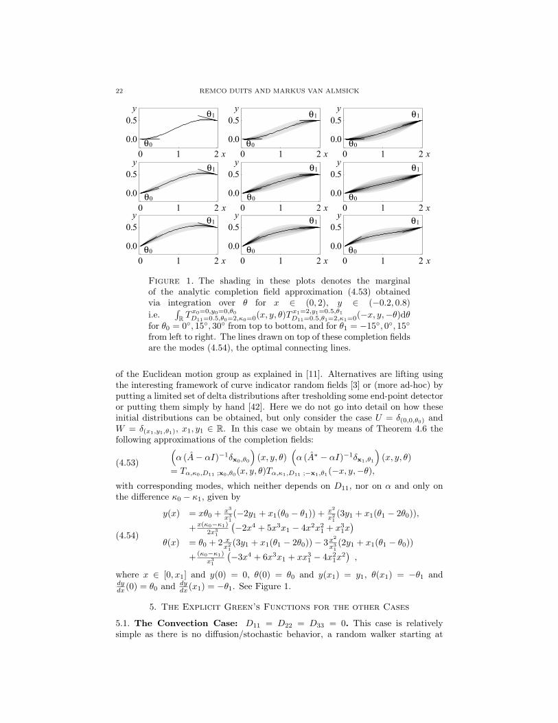


![Free – Boundary Linear Parameterization of 3D …sjg/papers/nonConv.pdfthat of Desbrun et al. [1] that works only for triangle meshes. In this method, explicit linear conditions](https://static.documents.pub/doc/80x56/5f744cf8a26ac43c1f7838d4/free-a-boundary-linear-parameterization-of-3d-sjgpapersnonconvpdf-that-of-desbrun.jpg)


