The future of health and long-term care spending - OECD.org · OECD Journal: Economic Studies...

OECD Journal: Economic Studies

Volume 2014

© OECD 2015

61

The future of healthand long-term care spending

by

Christine de la Maisonneuve and Joaquim Oliveira Martins*

This paper proposes a new set of public health and long-term care expenditureprojections until 2060, following up on the previous set of projections publishedin 2006. It disentangles health from long-term care expenditure as well as thedemographic from the non-demographic drivers, and refines the previousmethodology, in particular by better identifying the underlying determinants ofhealth and long-term care spending and by extending the country coverage toinclude BRIICS countries. A cost-containment and a cost-pressure scenario areprovided together with sensitivity analysis. On average across OECD countries,total health and long-term care expenditure is projected to increase by 3.3 and7.7 percentage points of GDP between 2010 and 2060 in the cost-containment andthe cost-pressure scenarios, respectively. For the BRIICS over the same period, it isprojected to increase by 2.8 and 7.3 percentage points of GDP in the cost-containment and the cost-pressure scenarios, respectively.

JEL classification codes: H51, I12, J11, J14.

Keywords: Public health expenditures, long-term care expenditures, ageingpopulations, longevity, demographic and non-demographic effects, projectionmethods.

* The authors are, respectively, members of the Economics Department and the Directorate for PublicGovernance and Territorial Development. Correspondence: [email protected] [email protected]. They would like to thank Jørgen Elmeskov, Fabrice Murtin,Giuseppe Nicoletti and Jean-Luc Schneider as well as their colleagues from the Health Division ofthe Directorate for Employment, Labour and Social Affairs for their valuable comments on an earlierdraft of the paper. They are also grateful to Luca Lorenzoni, Fabio Pammolli and Yuki Murakami fortheir thorough reading of the paper and their useful suggestions. Special thanks go toInes Gomez Palacio for excellent technical and editing assistance. The views expressed in this paperare those of the authors and do not necessarily reflect those of the OECD and its member countries.

The statistical data for Israel are supplied by and under the responsibility of the relevant Israeliauthorities. The use of such data by the OECD is without prejudice to the status of the Golan Heights,East Jerusalem and Israeli settlements in the West Bank under the terms of international law.

http://mailto:[email protected]

http://mailto:[email protected]

THE FUTURE OF HEALTH AND LONG-TERM CARE SPENDING

OECD JOURNAL: ECONOMIC STUDIES – VOLUME 2014 © OECD 201562

1. IntroductionSpending on health and long-term care (henceforth LTC) is a first-order policy issue for

most governments in OECD countries. These expenditures are putting pressure on public

budgets, adding to that arising from other social spending programmes and, once interest

rates normalise, servicing of higher debt levels than in the past. The ratio of public health

and LTC expenditure to GDP1 has been rising steadily for several decades. Since 1970, on

average across OECD countries, the expenditure to GDP ratio has increased by

3.5 percentage points to reach around 7 percentage points in 2010. Interestingly, this ratio

tends to increase during recession periods meaning that health expenditure keeps on

rising while GDP stagnates or decreases (Figure 1). Despite a recent slowdown, as a share of

GDP, public health and long-term care expenditure have still increased by slightly less than

1 percentage point from the level prior to the crisis.

Looking towards the future, the OECD (2006) public health and LTC spending

projections highlighted the growing pressures over the next 50 years. In an upside “cost-

pressure” scenario, average health and LTC expenditure was projected to almost double

again, to reach approximately 13% of GDP by 2050. But, even in the so-called “cost-

containment” scenario, spending was still projected to rise to approximately 10% of GDP on

average across OECD countries over the next 50 years. Comparing the 2006 OECD

projections with actual data up to 2010 (Figure 2, panel A), the observed increase in the

ratio of public health and LTC spending to GDP was above even the pessimistic “cost-

pressure scenario”. On average for OECD countries, these expenditures have represented

an increasing share of total public expenditures (Figure 2, panel B).

Figure 1. Evolution of public health and long-term care expenditure1

As a % of GDP

1. Unweighted average of available OECD countries.Source: OECD Health Database (2012).

8.0

7.5

7.0

6.5

6.0

5.5

5.0

4.5

4.0

3.5

3.0

1970

1972

1974

1976

1978

1980

1982

1984

1986

1988

1990

1992

1994

1996

1998

2000

2002

2004

2006

2008

2010


OECD JOURNAL: ECONOMIC STUDIES – VOLUME 2014 © OECD 2015 63

The projections in this paper update and refine the OECD (2006) analysis by extending

the country coverage and improving the method of estimating future developments in

health and LTC expenditure. In addition to the 34 OECD countries, health and LTC

expenditure is also projected for Brazil, China, India, Indonesia, Russia and South Africa

(henceforth BRIICS). Concerning the methodology, as in 2006, the new projections separate

health and LTC and, within each type of expenditure, demographic from non-demographic

drivers. For health care, the main difference concerns the non-demographic drivers, with

an attempt to better understand the residual expenditure growth by determining which

share can be explained by the evolution of health prices and technology effects. Regarding

LTC, a more precise estimation of the determinants of the number of dependants (people

needing help in their daily life activities) is provided. In particular, the current set of

projections treats health expenditure itself as a determinant of the dependency ratios

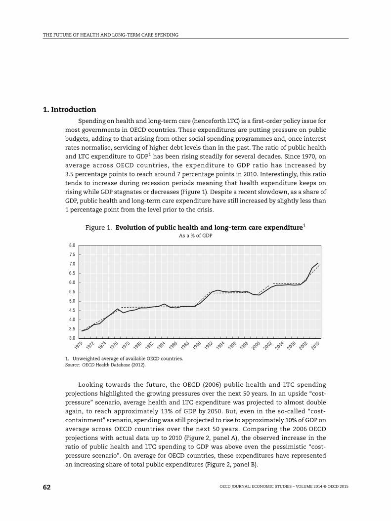
Figure 2. Evolution of public health and long-term care expenditures1

1. Unweighted average of available OECD countries.2. The trend GDP was derived from the OECD Economic Outlook Database.Source: OECD Health Database (2011), OECD (2006), OECD Economic Outlook Database, No. 91.

6.9

6.7

6.5

6.3

6.1

5.9

5.7

5.5

2000

2001

2002

2003

2004

2005

2006

2007

2008

2009

2010

16.0

15.5

15.0

14.5

13.5

14.0

13.0

12.5

12.0

2000

1990

1991

1992

1993

1994

1995

1996

1997

1998

1999

2001

2002

2003

2004

2005

2006

2007

2008

2009

2010

OECD average 2006 cost-containment scenario 2006 cost-pressure scenario

A. Comparison of actual development and OECD (2006) projectionsIn % of trend GDP2

B. Share of health and LTC spending in total public spendingIn % of total public expenditure



(number of dependent people in total population) by age groups. Finally, the new

projections extend to 2060.

The projections are provided for public expenditure only. Nonetheless, the cross-

country differences in treatment of tax expenditures,2 which can be large in some cases, may

introduce serious bias in the split between public and private expenditures. Indeed,

countries interpret differently the OECD manual on the System of Health accounts on how to

deal with tax expenditures. Australia and Germany, for instance, deduct tax expenditures

from private insurance expenditures and report it as public expenditure. But, in the United

States, tax expenditures are not considered as public expenditure (OECD, 2010).

The paper is set out as follows. In Section 2, the main demographic and non-

demographic drivers of public health expenditure are analysed and projected over the next

half century. Cost-containment (with implicit policy actions) and cost-pressure (without

policy actions) scenarios are presented, followed by a discussion of the sensitivity of the

results to key assumptions. In Section 3, the same sequence applies to public LTC

expenditures. In Section 4, different health and LTC expenditure scenarios are combined in

order to provide a range of estimates for total expenditure. Section 5 concludes.

2. Health care

2.1. The determinants of public health care expenditure

The drivers of public health care expenditure are demographic and non-demographic

(Figure 3). Demographic drivers relate broadly to the age structure of the population and

the evolution of its health status, while a non-demographic driver is income. The

relationship between health expenditures and income remains an unsettled issue, but

independent of the precise income elasticity (measure of the responsiveness of health

expenditure to a change in income) the combination of demographic and income effects

fails to explain a large part of the total growth in public health-care expenditure in the past.

Thus, a residual unexplained growth remains. Relative prices, technological progress and

the underlying health policies and institutions are the most likely candidates for

explaining this residual (see Box 3 in de la Maisonneuve and Oliveira Martins, 2013).

To quantify the relative contribution of each driver over the past 15 years, a simple

accounting analysis was carried out (for data sources and methodology, see Annex A). The

analysis accounts for changes in the population structure during the period 1995-2009, and

assumes an income elasticity of health spending of either 0.8 or 1 (see below for a

discussion of this hypothesis). Based on these assumptions an expenditure residual was

derived. As can be seen from Table 1, demographic drivers explain relatively little of past

Figure 3. The determinants of public health expenditure

Health careexpenditure

Demography

Agestructure

Healthby age

Income Residual

Relativeprices Technology

Institutionsand policies



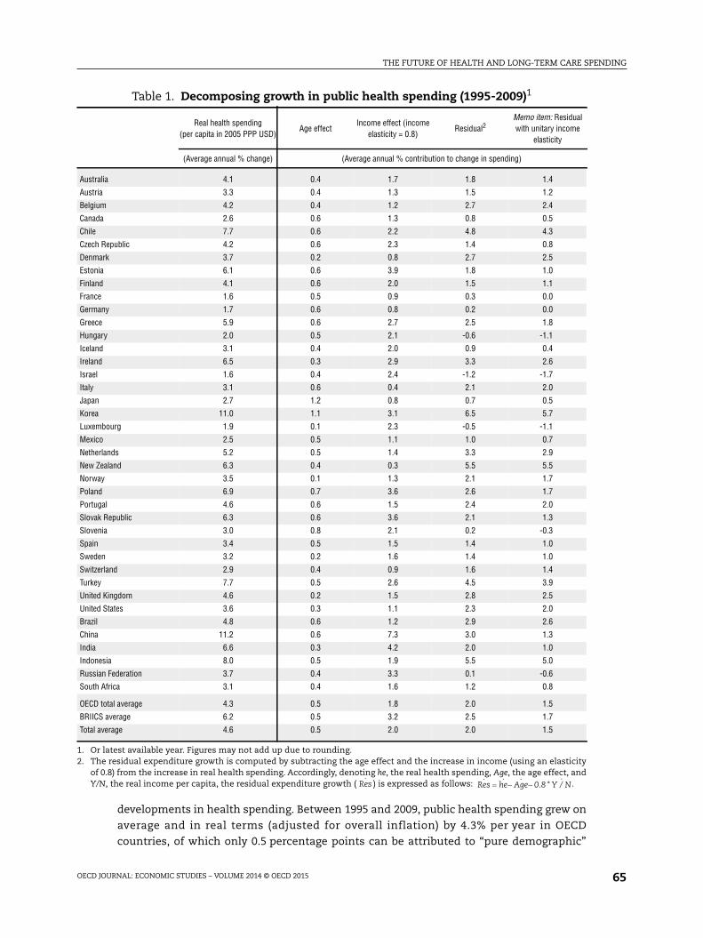
developments in health spending. Between 1995 and 2009, public health spending grew on

average and in real terms (adjusted for overall inflation) by 4.3% per year in OECD

countries, of which only 0.5 percentage points can be attributed to “pure demographic”

Table 1. Decomposing growth in public health spending (1995-2009)1

Real health spending(per capita in 2005 PPP USD)

Age effectIncome effect (income

elasticity = 0.8)Residual2

Memo item: Residualwith unitary income

elasticity

(Average annual % change) (Average annual % contribution to change in spending)

Australia 4.1 0.4 1.7 1.8 1.4

Austria 3.3 0.4 1.3 1.5 1.2

Belgium 4.2 0.4 1.2 2.7 2.4

Canada 2.6 0.6 1.3 0.8 0.5

Chile 7.7 0.6 2.2 4.8 4.3

Czech Republic 4.2 0.6 2.3 1.4 0.8

Denmark 3.7 0.2 0.8 2.7 2.5

Estonia 6.1 0.6 3.9 1.8 1.0

Finland 4.1 0.6 2.0 1.5 1.1

France 1.6 0.5 0.9 0.3 0.0

Germany 1.7 0.6 0.8 0.2 0.0

Greece 5.9 0.6 2.7 2.5 1.8

Hungary 2.0 0.5 2.1 -0.6 -1.1

Iceland 3.1 0.4 2.0 0.9 0.4

Ireland 6.5 0.3 2.9 3.3 2.6

Israel 1.6 0.4 2.4 -1.2 -1.7

Italy 3.1 0.6 0.4 2.1 2.0

Japan 2.7 1.2 0.8 0.7 0.5

Korea 11.0 1.1 3.1 6.5 5.7

Luxembourg 1.9 0.1 2.3 -0.5 -1.1

Mexico 2.5 0.5 1.1 1.0 0.7

Netherlands 5.2 0.5 1.4 3.3 2.9

New Zealand 6.3 0.4 0.3 5.5 5.5

Norway 3.5 0.1 1.3 2.1 1.7

Poland 6.9 0.7 3.6 2.6 1.7

Portugal 4.6 0.6 1.5 2.4 2.0

Slovak Republic 6.3 0.6 3.6 2.1 1.3

Slovenia 3.0 0.8 2.1 0.2 -0.3

Spain 3.4 0.5 1.5 1.4 1.0

Sweden 3.2 0.2 1.6 1.4 1.0

Switzerland 2.9 0.4 0.9 1.6 1.4

Turkey 7.7 0.5 2.6 4.5 3.9

United Kingdom 4.6 0.2 1.5 2.8 2.5

United States 3.6 0.3 1.1 2.3 2.0

Brazil 4.8 0.6 1.2 2.9 2.6

China 11.2 0.6 7.3 3.0 1.3

India 6.6 0.3 4.2 2.0 1.0

Indonesia 8.0 0.5 1.9 5.5 5.0

Russian Federation 3.7 0.4 3.3 0.1 -0.6

South Africa 3.1 0.4 1.6 1.2 0.8

OECD total average 4.3 0.5 1.8 2.0 1.5

BRIICS average 6.2 0.5 3.2 2.5 1.7

Total average 4.6 0.5 2.0 2.0 1.5

1. Or latest available year. Figures may not add up due to rounding.2. The residual expenditure growth is computed by subtracting the age effect and the increase in income (using an elasticity

of 0.8) from the increase in real health spending. Accordingly, denoting he, the real health spending, Age, the age effect, andY/N, the real income per capita, the residual expenditure growth ( ) is expressed as follows: .Res

.Res he Age Y N

. . . . 0 8. * /



developments. Assuming an income elasticity equal to 0.8, income effects add

1.7 percentage points of growth on top of the 0.5 percentage points attributable to

demographics. Therefore, a residual growth can be estimated at around 2 percentage

points per year on average across OECD countries, with the BRIICS experiencing even more

important residual growth effects. With an income elasticity of one, the residual on

average for the OECD would still be around 1.5% per year. Only with a somewhat unrealistic

income elasticity of 1.8, demographic and income effects could explain most of the

observed expenditure growth.

The calculated expenditure residual growth displays large differences across countries

(Figure 4). It ranges from above 5% per year for countries such as Korea and New Zealand,

to values well below 0.5% for France, Germany, Slovenia and Russia, and is even negative

for Israel. Extrapolating these country-specific idiosyncrasies over the next 50 years may

generate unreliable results as most of them would lead to unsustainable expenditure

ratios. For this reason, in this study, it was preferred to use a common average residual

growth (see below).

2.2. Projection framework

The framework used to project public health expenditure combines both the

demographic and non-demographic drivers described above. The evolution of each driver

is first projected separately, and subsequently combined to compute the future growth of

total health expenditure. Thus, the evolution of the future share of public health care

spending in GDP depends on demographic and real income per capita projections, as well

as on the extrapolated residual growth component. The demographic driver includes three

elements – death-related costs, pure age effects based on population projections drawn

from different sources and a healthy-ageing effect – which are described below. Future GDP

is based on projections published in the OECD Economic Outlook, No. 91.3 As in the historical

Figure 4. Health care residual expenditure growth by country (1995-2009)Annual average growth rates in %

1. Unweighted average.Source: OECD Health Database (2011) and authors’ calculations.

6.8

5.8

4.8

3.8

2.8

1.8

0.8

-0.2

-1.2

%

Korea

New Ze

aland

Indon

esia

Chile

Turke

y

Irelan

d

Netherl

andsChin

aBraz

il

United

Kingdo

m

Denmark

Belgium

Poland

Greece

BRIICS av

erag

e1

Portug

al

United

States

Slovak

Rep

ublic Ita

ly

Norway

India

OECD av

erag

e1

Austra

lia

Eston

ia

Switzerl

and

Finlan

d

Austri

a

SwedenSpa

in

Czech

Rep

ublic

South

Africa

Mexico

Icelan

d

Canad

aJa

pan

Franc

e

German

y

Sloven

ia

Russia

n Fed

eratio

n

Luxe

mbourg

Hunga

ryIsr

ael



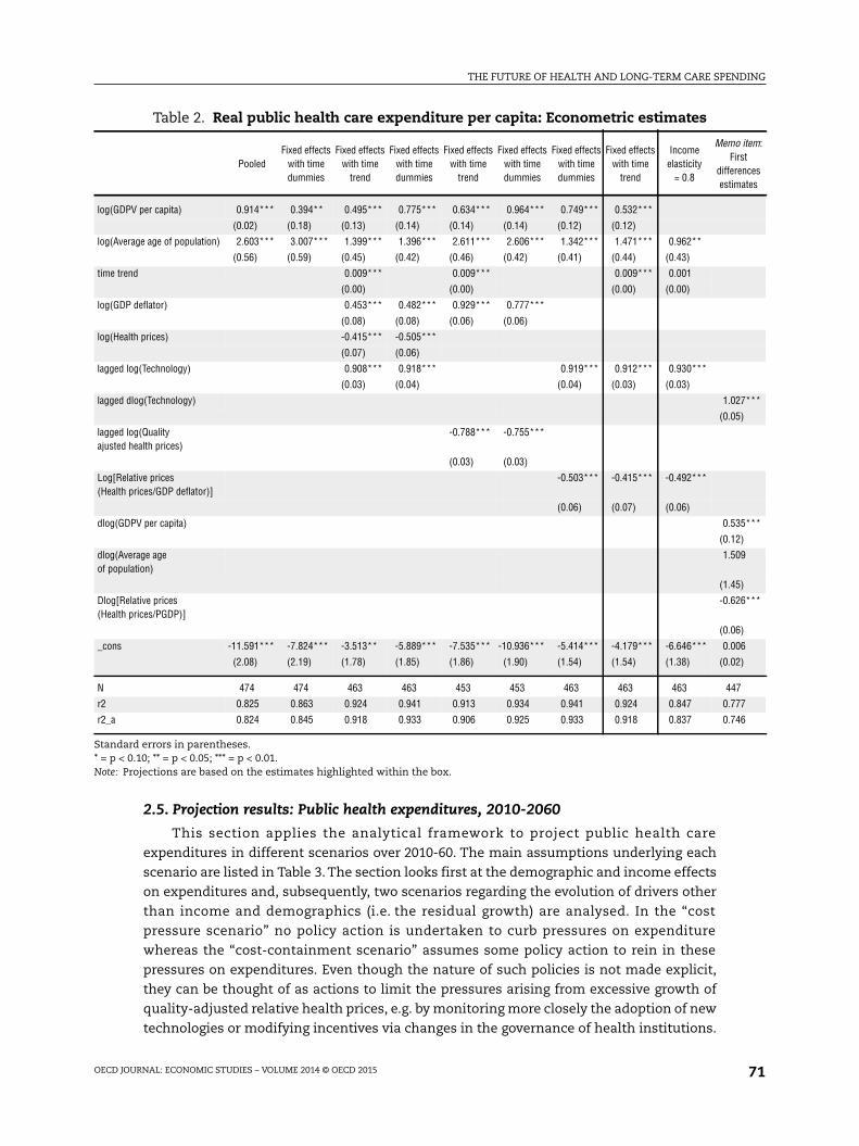
accounting exercise, the income effects are captured by an elasticity of health

expenditures that can take the value of 0.8 or 1, depending on the scenario.

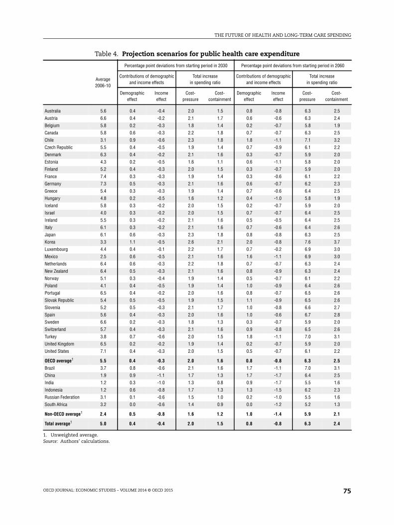
The growth rates in spending ratios are first projected for each country and they are

then adjusted to allow for a certain convergence across countries towards a common target

level. Ceteris paribus, countries having a below-average initial level of public health

expenditure to GDP ratios are projected to experience higher growth rates than those close

to the average. This makes the projections more comparable across countries, as the

effects of the different mechanisms at work during the projection period are isolated from

the impact of the initial conditions. This is particularly important in the context of a

projection method that does not assume country-specific residual growth in expenditures

(as in the baseline assumed in this paper), or for countries that have in the base year a very

low level of spending, such as emerging economies.

Therefore, the projected (for period t) health spending ratios were adjusted as follows:

where gi is the growth rate of health spending for country i (from period 0 to period t);

is the health expenditure ratio for country i in the base period; and is the

health expenditure ratio for the OECD average in the base period.

When the spending ratio of a given country is below (or above) the OECD average for

the base year this adjustment will increase (decrease) the projected growth rate of

expenditures to GDP, thus allowing for convergence to take place. In order to smooth out

the impact of the recent crisis on expenditure, the base year spending ratios are computed

as the average shares of public health care spending in GDP over 2006-10. This framework

is used to project public health care expenditures over the period 2010-60.

The base information used to construct the health expenditure projection framework

is the average health expenditure profile by age group (Figure 5). Average health

Figure 5. Public health care expenditure by age groups1

% of GDP per capita

1. The graph shows the dispersion of health care expenditure across countries by age groups. The diamondsrepresent the median. The boxes are the 2nd and 3rd quartiles of the distribution of expenditure across countries.The whiskers are the 1st and 4th quartiles.

Source: European Commission, 2009 Ageing Report: Economic and Budgetary Projections for the EU27 Member States (2008-60).

HEY

HE Y

HE Yg

HE..i t

OECD

i

i

,

,

,

/

/1 0

0YY i

,0

HEY i

,0

HEY OECD

,0

30

20

10

0

2 7 12 17 22 27 32 37 42 47 52 57 62 67 72 77 82 87 92 97Age (middle of 5-years age brackets)

% of GDP per capita



expenditures are relatively high for young children; they decrease and remain stable for

most of the prime-age period, and then start to increase rapidly in older age, the health

care cost of people aged 90 and over being six times that of young people. Until the age

of 65, health expenditure profiles are rather similar across countries, but from 65 onwards,

they display a large heterogeneity. The standard deviation by age group increases from

1.8% for the 65-69 age group to more than 5% for people aged 90 and over.

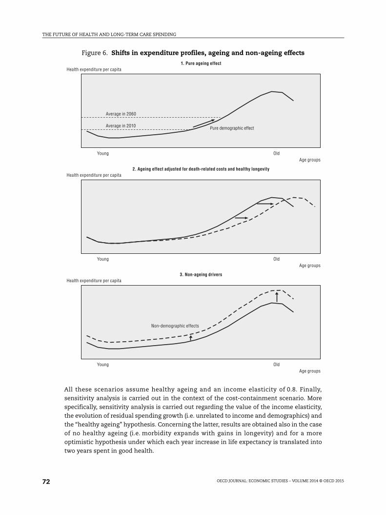
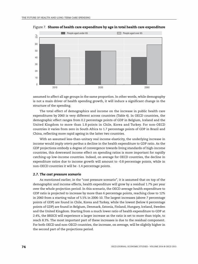
From Figure 5, it could be expected a priori that an ageing population would be

associated with increasing aggregate per capita public health care expenditures: the fact

that the share of older people in the population is growing faster than that of any other age

group, both as a result of longer lives and a lower birth rate, should generate an automatic

increase in the average. However, this intuition finds little support in the data and

assessing the effect of population ageing on health and health care has proved to be far

from straightforward (Breyer et al., 2011).

Consistent with a large number of previous studies (Felder et al., 2000; Seshamani and

Gray, 2004; Breyer and Felder, 2006; and Werblow et al., 2007; etc.), this paper assumes that

what matters for health spending is not ageing but rather the proximity to death, i.e. the

so-called “death-related costs” (DRC) hypothesis. This interpretation is consistent with the

observed facts that health-care expenditure tends to increase in a disproportionate way

when individuals are close to death, and mortality rates are obviously higher for older

people. When the projected increase in life expectancy is accompanied by an equivalent

gain in the number of years spent in good health, the health care spending is only driven

by the proximity to death and not by an increase in the average age of the population. In

other words, it is not ageing per se that pushes up average health expenditures, but rather

the fact that mortality rates increase with age. The death-related costs hypothesis is,

therefore, consistent with a so-called healthy-ageing regime, where longevity gains are all

translated into years in good health (Box 1).

Box 1. Healthy ageing hypothesis

To take into account the “healthy ageing” hypothesis, the survivor expenditure curve isallowed to shift rightwards according to longevity gains, progressively postponing the age-related increases in expenditure. First, the curve by five-year age groups is interpolated inorder to derive a yearly age profile. In this way, the expenditure curve can be shiftedsmoothly over time, in line with life expectancy gains.

Subsequently, the shift of the curve can be simulated by subtracting the increase in lifeexpectancy at birth according to national projections from each current age. For example,a 70-year old person in Germany is projected to have the health status of a 67-year oldperson by 2025 and that of a 64-year old person by 2050.

By contrast, in a “pure demographic” scenario, the expenditure curves would not shiftrightwards with ageing, reflecting the implicit assumption of unchanged health status atany given age. When these curves stay put in the presence of longevity gains, the share oflife lived in “bad health” increases with life expectancy.

It should be noted that the population projections used in the analysis are pre-determined and do not take into account the effect of health spending on health statusand longevity. Making population projections dependent on the level of health spending isbeyond the scope of this project and could be the object of further research.



To account for the dominance of death-related costs and the healthy-ageing regime, the

expenditure curve by age group needs to be split for each period into two segments of the

population: survivors and non-survivors. The non-survivors’ expenditure curve can be

estimated by multiplying the estimated health costs in the proximity to death by age group

by the number of deaths per age group. The “cost of death” was proxied here by the health

expenditure per capita for the oldest age group (95+) multiplied by a factor that captures the

tendency for the costs of death to be higher at younger ages. This factor is kept constant at 4

for people aged between 0 and 59 years and declines linearly (towards unity) afterwards.4

As regards non-survivors, two different demographic effects are at play. On the one

hand, the number of deaths is set to rise due to the transitory effect of the post-War baby-

boom. On the other hand, if mortality falls over time due to an ongoing increase in

longevity, fewer will be at the very end of life in each given year, thus mitigating health care

costs.5 The impact of demographic developments on public health care expenditures will

depend on the relative size of these effects.

In principle, the survivors’ expenditure curve for each country could be derived from

the difference between the total cost curve and that of the non-survivor. However, given

the uncertainties surrounding these data, it seemed preferable to estimate an average

expenditure curve for survivors, to be then used for all countries. In this way, the

projections are less sensitive to initial conditions and to country-specific data

idiosyncrasies. This expenditure curve for survivors was estimated econometrically as a

non-linear function of age. Each country-specific curve is then calibrated in order to fit the

base year of the projections.

2.3. Non-demographic drivers

As mentioned above, overall demographic drivers explain relatively little of past

developments in health spending, even assuming that the expenditure curve by age

remains constant (or abstracting from “healthy ageing” effects). Therefore, the non-

demographic drivers must play an important role: these are the growth in income and a

residual growth component.

The effect of real income growth on public health expenditures has been the subject

of a vast debate, but the precise value of the income elasticity is still uncertain. Empirical

estimates tend to increase with the degree of income aggregation, implying that health

care could be “an individual necessity and a national luxury” (Getzen, 2000). However, a

high aggregate income elasticity (above unity) often found in macro studies may result

from biases in estimates originating from a number of sources, such as failure to

appropriately control for quality effects and account for the peculiar statistical properties

of some of the variables. Based on the most recent findings from this literature

(e.g. Acemoglu et al., 2009; and Holly et al., 2011), as well as estimations carried out by the

authors, a real income elasticity equal to 0.8 has been used (a middle point across those

estimates) and the sensitivity of the projections to this assumption was subsequently

tested (by contrast, OECD, 2006 assumed a unitary income elasticity throughout).

Once income growth has been accounted for, several factors may explain the residual

growth observed in the past: developments in relative prices, technological progress and the

features of health institutions and policies (see Box 3 and Appendix 2 in de la Maisonneuve

and Oliveira Martins, 2013). It is not feasible at this stage to project these drivers individually.

Nonetheless, in an attempt to interpret this residual growth, an econometric equation has



been estimated, incorporating explicitly the effects of prices and a proxy for quality.

Accordingly, the income elasticity (), as well as the price () and quality () elasticities, were

derived from a panel regression (in log terms and expressed in quality-adjusted health

volumes per capita), augmented with the drift factors related to demography and exogenous

policy factors captured by a time trend (e.g. institutional reforms increasing the coverage of

the health coverage system):

where he denotes health care demand volumes (deflated for price and quality), N is total

population, Age is the average age of the population, P are health care prices, PY is the GDP

factor, Q is a quality index for health care products and Y is real GDP; αc correspond to

country fixed-effects; T to a time trend; and u a randomly distributed residual. The

equation was estimated both in levels and in first differences. The demographic effect is

captured by the average age of the population. The quality effect (Q) was loosely proxied by

a ratio involving the relative pace of patent creation in the health sector compared with the

rest of the economy for the average of OECD countries. This ratio is assumed to represent

the change in the technology frontier. To capture country-specific effects related to the

diffusion and adoption of technology, the ratio is multiplied by the share of R&D

expenditures in GDP.

The results of the econometric estimation are relatively robust, with the value of the

income elasticity fluctuating from around 0.5 to close to 1, depending on the

specifications. The preferred econometric estimate (column 8 of Table 2) gives an

estimated elasticity of 0.42 for relative prices (β) and 0.91 for the technology/quality effect

(γ). Translating these into expenditure elasticities, (β + 1) and (1 – γ), and the observed

growth rates of (P/PY) and (Q) the overall effect of technology and relative prices is

estimated to have increased health-care expenditures by 0.8% per year. In other words, the

econometric model is able to explain more than one-third of the past expenditure residual

of 2% per year for the OECD average, displayed in Table 1. Estimates suggest that the

residual expenditure is also driven by other factors, such as changes in policy and

institutions which can be loosely captured by a time trend. These other factors account for

0.9% of the increase in health expenditure per year. Overall, these estimates suggest that

the residual expenditure has increased health-care expenditures by around 1.7%

(i.e. 0.8% + 0.9%) per year.6

As stated previously, a common residual growth is assumed for all countries in order not

to extrapolate country-specific idiosyncrasies over a long period. Based on the estimates of

Table 2, the projections assume a uniform residual expenditure growth of 1.7% per year.

2.4. Summing upTo summarise graphically the way in which demographic and non-demographic

drivers contribute to health care spending (Figure 6), the mechanical effect of population

ageing on expenditures can be displayed as moving up along the expenditure curve,

assuming that the age profile of expenditures remains constant over time (Panel 1). This

age factor is then adjusted by incorporating the healthy ageing hypothesis, corresponding

to a rightward shift of the curve (Panel 2). This shift implies that older people still cost more

than the young, but at progressively older ages. Finally, the expenditure curve may shift

upwards7 (Panel 3) due to non-demographic drivers (income, the quality-adjusted relative

health prices and other unexplained factors, such as policies and institutions).

logheN

log(Age) logPP

log(Q) logcY

YYN

T u

. . . . .



2.5. Projection results: Public health expenditures, 2010-2060

This section applies the analytical framework to project public health care

expenditures in different scenarios over 2010-60. The main assumptions underlying each

scenario are listed in Table 3. The section looks first at the demographic and income effects

on expenditures and, subsequently, two scenarios regarding the evolution of drivers other

than income and demographics (i.e. the residual growth) are analysed. In the “cost

pressure scenario” no policy action is undertaken to curb pressures on expenditure

whereas the “cost-containment scenario” assumes some policy action to rein in these

pressures on expenditures. Even though the nature of such policies is not made explicit,

they can be thought of as actions to limit the pressures arising from excessive growth of

quality-adjusted relative health prices, e.g. by monitoring more closely the adoption of new

technologies or modifying incentives via changes in the governance of health institutions.

Table 2. Real public health care expenditure per capita: Econometric estimates

PooledFixed effects

with timedummies

Fixed effectswith time

trend

Fixed effectswith timedummies


trend




trend

Incomeelasticity

= 0.8

Memo item:First

differencesestimates

log(GDPV per capita) 0.914*** 0.394** 0.495*** 0.775*** 0.634*** 0.964*** 0.749*** 0.532***

(0.02) (0.18) (0.13) (0.14) (0.14) (0.14) (0.12) (0.12)

log(Average age of population) 2.603*** 3.007*** 1.399*** 1.396*** 2.611*** 2.606*** 1.342*** 1.471*** 0.962**

(0.56) (0.59) (0.45) (0.42) (0.46) (0.42) (0.41) (0.44) (0.43)

time trend 0.009*** 0.009*** 0.009*** 0.001

(0.00) (0.00) (0.00) (0.00)

log(GDP deflator) 0.453*** 0.482*** 0.929*** 0.777***

(0.08) (0.08) (0.06) (0.06)

log(Health prices) -0.415*** -0.505***

(0.07) (0.06)

lagged log(Technology) 0.908*** 0.918*** 0.919*** 0.912*** 0.930***

(0.03) (0.04) (0.04) (0.03) (0.03)

lagged dlog(Technology) 1.027***

(0.05)

lagged log(Qualityajusted health prices)

-0.788*** -0.755***

(0.03) (0.03)

Log[Relative prices(Health prices/GDP deflator)]

-0.503*** -0.415*** -0.492***

(0.06) (0.07) (0.06)

dlog(GDPV per capita) 0.535***

(0.12)

dlog(Average ageof population)

1.509

(1.45)

Dlog[Relative prices(Health prices/PGDP)]

-0.626***

(0.06)

_cons -11.591*** -7.824*** -3.513** -5.889*** -7.535*** -10.936*** -5.414*** -4.179*** -6.646*** 0.006

(2.08) (2.19) (1.78) (1.85) (1.86) (1.90) (1.54) (1.54) (1.38) (0.02)

N 474 474 463 463 453 453 463 463 463 447

r2 0.825 0.863 0.924 0.941 0.913 0.934 0.941 0.924 0.847 0.777

r2_a 0.824 0.845 0.918 0.933 0.906 0.925 0.933 0.918 0.837 0.746

Standard errors in parentheses.* = p < 0.10; ** = p < 0.05; *** = p < 0.01.Note: Projections are based on the estimates highlighted within the box.



All these scenarios assume healthy ageing and an income elasticity of 0.8. Finally,

sensitivity analysis is carried out in the context of the cost-containment scenario. More

specifically, sensitivity analysis is carried out regarding the value of the income elasticity,

the evolution of residual spending growth (i.e. unrelated to income and demographics) and

the “healthy ageing” hypothesis. Concerning the latter, results are obtained also in the case

of no healthy ageing (i.e. morbidity expands with gains in longevity) and for a more

optimistic hypothesis under which each year increase in life expectancy is translated into

two years spent in good health.

Figure 6. Shifts in expenditure profiles, ageing and non-ageing effects

Age groupsYoung Old

Health expenditure per capita 1. Pure ageing effect

Age groupsYoung Old

Age groups

Health expenditure per capita 2. Ageing effect adjusted for death-related costs and healthy longevity

Young Old

Health expenditure per capita 3. Non-ageing drivers

Average in 2060

Average in 2010 Pure demographic effect

Non-demographic effects



2.6. Demographic and income effects

As discussed above, demographic effects on public health care expenditures can be

decomposed into health care costs for survivors, the adjustment for “healthy ageing” and

death-related costs. The pure ageing effect can be quite large in some countries, but tends

to be compensated by better health status. Whereas on a per capita basis death-related

costs account for the largest part of lifetime expenditures, for the population as a whole

they account for only a small fraction of the increase in expenditures as a share of GDP

since they concern only the non-survivors.

On average, the demographic effect only accounts for a small increase in expenditure.

In OECD countries and on its own, it pushes spending from 5.5% of GDP on average to 6.2%

in 2060. In non-OECD countries, the demographic effect on its own increases spending

from 2.4% of GDP to 3.4% in 2060. While the “healthy ageing” assumption may render the

simulation of demographic effects relatively optimistic, this is in line with observed

patterns of health status regimes in many OECD countries. It is assumed that the same

pattern will apply to non-OECD countries. The effect is projected to apply evenly before and

after 2030 for both OECD and non-OECD countries.

It is noteworthy that while demography is not a main driver of health care spending

growth, it will induce a significant change in the structure of spending over time. In 2010,

60% of health care expenditures were directed to people below 65 years old. In 2060,

roughly the same percentage of expenditures will be directed to people aged above 65,

reflecting an increase from 15% to 30% of their share in total population (Figure 7). This

evolution is only the consequence of demographic effects as non-demographic effects are

Table 3. Assumptions underlying the alternative projection scenarios: Public health care

Scenarios Health status Income elasticity Non-demographic, non-income drivers

Demographic effect Healthy ageing: Longevity gains aretranslated into equivalent additional

years in good health.

n.a. n.a.

Cost-pressure scenario Healthy ageing: Longevity gains aretranslated into equivalent additional


Income elasticity = 0.8 The residual is assumed to growat 1.7% over the projection period.

Cost-containment scenario Healthy ageing: Longevity gains aretranslated into equivalent additional


Income elasticity = 0.8 The residual growth is 1.7% in thestarting period and then converges

to 0 in 2060.

Sensitivity analysis based on the cost-containment scenario

Compression of morbidity Longevity gains are doubled intoadditional years in good health.


to 0 in 2060.

Expansion of morbidity No healthy ageing adjustment,i.e. longevity gains do not translateinto additional years in good health.


to 0 in 2060.

Country-specific quality adjustedrelative prices

Healthy ageing: Longevity gains aretranslated into equivalent additional


Income elasticity = 0.8 The residual growth is country specificand converges to 0 in 2060.

Income elasticity = 0.6 Healthy ageing: Longevity gains aretranslated into equivalent additional



to 0 in 2060.

Income elasticity = 1 Healthy ageing: Longevity gains aretranslated into equivalent additional


Income elasticity = 1 The residual growth is 1.7% in thestarting period and then converges

to 0 in 2060.

Note: The key assumption changed in each scenario is in bold.



assumed to affect all age groups in the same proportion. In other words, while demography

is not a main driver of health spending growth, it will induce a significant change in the

structure of the spending.

The total effect of demographics and income on the increase in public health care

expenditures by 2060 is very different across countries (Table 4). In OECD countries, the

demographic effect ranges from 0.2 percentage points of GDP in Belgium, Iceland and the

United Kingdom to more than 1.8 points in Chile, Korea and Turkey. For non-OECD

countries it varies from zero in South Africa to 1.7 percentage points of GDP in Brazil and

China, reflecting more rapid ageing in the latter two countries.

With an assumed less-than-unitary real income elasticity, the underlying increase in

income would imply ceteris paribus a decline in the health expenditure to GDP ratio. As the

GDP projections embody a degree of convergence towards living standards of high-income

countries, this downward income effect on spending ratios is more important for rapidly

catching-up low-income countries. Indeed, on average for OECD countries, the decline in

expenditure ratios due to income growth will amount to -0.8 percentage points, while in

non-OECD countries it will be -1.4 percentage points.

2.7. The cost pressure scenario

As mentioned earlier, in the “cost pressure scenario”, it is assumed that on top of the

demographic and income effects, health expenditure will grow by a residual 1.7% per year

over the whole projection period. In this scenario, the OECD average health expenditure to

GDP ratio is projected to increase by more than 6 percentage points, reaching close to 12%

in 2060 from a starting value of 5.5% in 2006-10. The largest increases (above 7 percentage

points of GDP) are found in Chile, Korea and Turkey, while the lowest (below 6 percentage

points of GDP) are found in Belgium, Denmark, Estonia, Finland, Hungary, Iceland, Sweden

and the United Kingdom. Starting from a much lower ratio of health expenditure to GDP at

2.4%, the BRIICS will experience a larger increase as the ratio is set to more than triple, to

reach 8.3%. The most important part of these increases is due to the residual component.

For both OECD and non-OECD countries, the increase, on average, will be slightly higher in

the second part of the projections period.

Figure 7. Shares of health care expenditure by age in total health care expenditure

70

60

50

40

30

20

10

0

%

2010 2030 2060

People aged under 65 People aged over 65



Table 4. Projection scenarios for public health care expenditure

Average2006-10

Percentage point deviations from starting period in 2030 Percentage point deviations from starting period in 2060

Contributions of demographicand income effects

Total increasein spending ratio

Contributions of demographicand income effects

Total increasein spending ratio

Demographiceffect

Incomeeffect

Cost-pressure

Cost-containment

Demographiceffect

Incomeeffect

Cost-pressure

Cost-containment

Australia 5.6 0.4 -0.4 2.0 1.5 0.8 -0.8 6.3 2.5

Austria 6.6 0.4 -0.2 2.1 1.7 0.6 -0.6 6.3 2.4

Belgium 5.8 0.2 -0.3 1.8 1.4 0.2 -0.7 5.8 1.9

Canada 5.8 0.6 -0.3 2.2 1.8 0.7 -0.7 6.3 2.5

Chile 3.1 0.9 -0.6 2.3 1.8 1.8 -1.1 7.1 3.2

Czech Republic 5.5 0.4 -0.5 1.9 1.4 0.7 -0.9 6.1 2.2

Denmark 6.3 0.4 -0.2 2.1 1.6 0.3 -0.7 5.9 2.0

Estonia 4.3 0.2 -0.5 1.6 1.1 0.6 -1.1 5.8 2.0

Finland 5.2 0.4 -0.3 2.0 1.5 0.3 -0.7 5.9 2.0

France 7.4 0.3 -0.3 1.9 1.4 0.3 -0.6 6.1 2.2

Germany 7.3 0.5 -0.3 2.1 1.6 0.6 -0.7 6.2 2.3

Greece 5.4 0.3 -0.3 1.9 1.4 0.7 -0.6 6.4 2.5

Hungary 4.8 0.2 -0.5 1.6 1.2 0.4 -1.0 5.8 1.9

Iceland 5.8 0.3 -0.2 2.0 1.5 0.2 -0.7 5.9 2.0

Israel 4.0 0.3 -0.2 2.0 1.5 0.7 -0.7 6.4 2.5

Ireland 5.5 0.3 -0.2 2.1 1.6 0.5 -0.5 6.4 2.5

Italy 6.1 0.3 -0.2 2.1 1.6 0.7 -0.6 6.4 2.6

Japan 6.1 0.6 -0.3 2.3 1.8 0.8 -0.8 6.3 2.5

Korea 3.3 1.1 -0.5 2.6 2.1 2.0 -0.8 7.6 3.7

Luxembourg 4.4 0.4 -0.1 2.2 1.7 0.7 -0.2 6.9 3.0

Mexico 2.5 0.6 -0.5 2.1 1.6 1.6 -1.1 6.9 3.0

Netherlands 6.4 0.6 -0.3 2.2 1.8 0.7 -0.7 6.3 2.4

New Zealand 6.4 0.5 -0.3 2.1 1.6 0.8 -0.9 6.3 2.4

Norway 5.1 0.3 -0.4 1.9 1.4 0.5 -0.7 6.1 2.2

Poland 4.1 0.4 -0.5 1.9 1.4 1.0 -0.9 6.4 2.6

Portugal 6.5 0.4 -0.2 2.0 1.6 0.8 -0.7 6.5 2.6

Slovak Republic 5.4 0.5 -0.5 1.9 1.5 1.1 -0.9 6.5 2.6

Slovenia 5.2 0.5 -0.3 2.1 1.7 1.0 -0.8 6.6 2.7

Spain 5.6 0.4 -0.3 2.0 1.6 1.0 -0.6 6.7 2.8

Sweden 6.6 0.2 -0.3 1.8 1.3 0.3 -0.7 5.9 2.0

Switzerland 5.7 0.4 -0.3 2.1 1.6 0.9 -0.8 6.5 2.6

Turkey 3.8 0.7 -0.6 2.0 1.5 1.8 -1.1 7.0 3.1

United Kingdom 6.5 0.2 -0.2 1.9 1.4 0.2 -0.7 5.9 2.0

United States 7.1 0.4 -0.3 2.0 1.5 0.5 -0.7 6.1 2.2

OECD average1 5.5 0.4 -0.3 2.0 1.6 0.8 -0.8 6.3 2.5

Brazil 3.7 0.8 -0.6 2.1 1.6 1.7 -1.1 7.0 3.1

China 1.9 0.9 -1.1 1.7 1.3 1.7 -1.7 6.4 2.5

India 1.2 0.3 -1.0 1.3 0.8 0.9 -1.7 5.5 1.6

Indonesia 1.2 0.6 -0.8 1.7 1.3 1.3 -1.5 6.2 2.3

Russian Federation 3.1 0.1 -0.6 1.5 1.0 0.2 -1.0 5.5 1.6

South Africa 3.2 0.0 -0.6 1.4 0.9 0.0 -1.2 5.2 1.3

Non-OECD average1 2.4 0.5 -0.8 1.6 1.2 1.0 -1.4 5.9 2.1

Total average1 5.0 0.4 -0.4 2.0 1.5 0.8 -0.8 6.3 2.4

1. Unweighted average.Source: Authors’ calculations.



2.8. The cost-containment scenario

While the cost-pressure projections may be useful as a benchmark, they do not seem

very plausible. It is unlikely that public health-care expenditures to GDP could continue to

grow at such rates, without limit. For instance, regarding drugs, the following policies can

help containing the costs: a more intense use of generics, a revision of reimbursement

practices for drugs with low medical service (and more stringent restrictions on exemptions

to this rule), a more frequent re-evaluation of prices of new drugs (in general a more

transparent and dynamic pricing of new drugs), centralised bargaining for the purchase of

drugs and medical goods in public hospitals, reduction in excessive consumption of specific

drugs. Regarding in-patient care, shorter length of stay, development of ambulatory

hospitalisation or more user choice among health providers could help reining in the

expenditure growth. Regarding out-patient care, a more stringent health monitoring of

patients affected by long-term diseases in order to reduce costly complications; financial

incentives set on general practitioners to reduce prescription inflation and enhance

prevention could also help in maintaining the health expenditure on a sustainable path.

Accordingly, a long-run convergence condition is considered in the cost-containment

scenario. Specifically, the growth contribution of the spending residual, whose past growth

was partly attributable to technology and relative price effects, is assumed to converge to zero

in 2060, implicitly representing the assumption that policies are more effective than in the past

in controlling the expenditure growth driven by non-demographic non-income related factors.

In this scenario (Table 4), the health expenditure to GDP ratio for OECD countries would

increase by 2.5 percentage points, to reach close to 8% on average by 2060. The largest

increases (above 3 percentage points of GDP) are found in Chile, Korea, Luxembourg, Mexico

and Turkey. The lowest increases (below 2 percentage points of GDP) are found in Estonia,

Hungary, Sweden and the United Kingdom. The increase in non-OECD countries averages

around 2 percentage points, to reach 4.5% of GDP by 2060. The effect of non-demographic

non-income factors is higher before 2030 than after for all countries, as the residual growth

is assumed to converge to zero over the projection period. The difference between cost-

pressure and cost-containment scenarios increases over time due to compounding effect of

the residual.

2.9. Sensitivity analysis

In the sensitivity analysis, a number of parameters were changed in the context of the

“cost-containment scenario”: the income elasticity, the residual spending growth, as well

as factors underlying health status at old age (Table 5). Overall, the previous results seem

relatively robust. Specifically, these alternative simulations do not change qualitatively the

picture emerging from the comparison of the “cost-pressure” and “cost-containment”

scenarios discussed above.

First, given that assumptions on the future evolution of the residual are necessarily

arbitrary, their impact on projections was checked by computing a cost-containment

scenario in line with the assumptions behind such a scenario in the previous 2006 OECD

projections. In this variant (not shown in the table), on top of the demographic and income

effects, the residual component is assumed to contribute 1% per year, tending towards 0%

in 2060. On average, the health expenditure to GDP ratio across OECD countries reaches

6.8% instead of 7.9% in this new exercise. For non-OECD countries, the ratio will reach 3.3%

instead of 4.4%. As the assumption underlying this scenario is common for all countries,



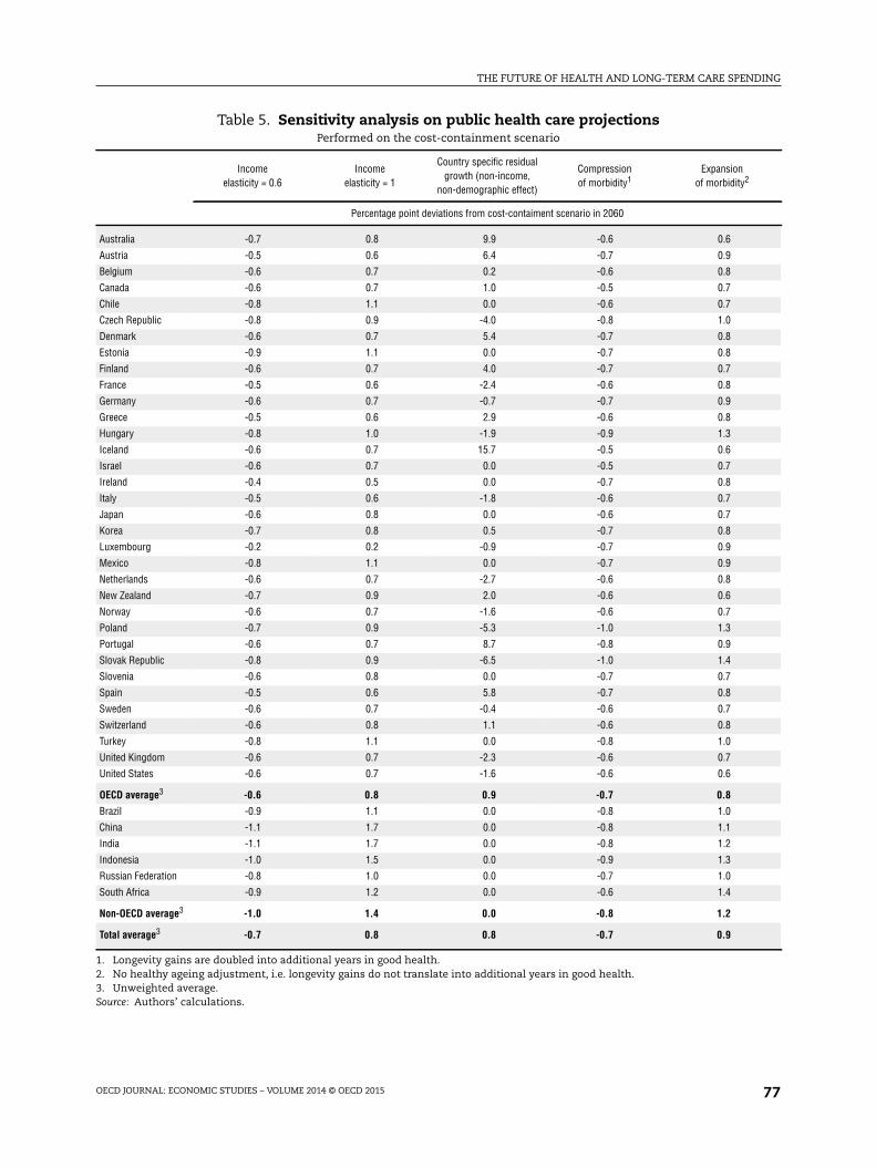
Table 5. Sensitivity analysis on public health care projectionsPerformed on the cost-containment scenario

Incomeelasticity = 0.6

Incomeelasticity = 1

Country specific residualgrowth (non-income,

non-demographic effect)

Compressionof morbidity1

Expansionof morbidity2

Percentage point deviations from cost-contaiment scenario in 2060

Australia -0.7 0.8 9.9 -0.6 0.6

Austria -0.5 0.6 6.4 -0.7 0.9

Belgium -0.6 0.7 0.2 -0.6 0.8

Canada -0.6 0.7 1.0 -0.5 0.7

Chile -0.8 1.1 0.0 -0.6 0.7

Czech Republic -0.8 0.9 -4.0 -0.8 1.0

Denmark -0.6 0.7 5.4 -0.7 0.8

Estonia -0.9 1.1 0.0 -0.7 0.8

Finland -0.6 0.7 4.0 -0.7 0.7

France -0.5 0.6 -2.4 -0.6 0.8

Germany -0.6 0.7 -0.7 -0.7 0.9

Greece -0.5 0.6 2.9 -0.6 0.8

Hungary -0.8 1.0 -1.9 -0.9 1.3

Iceland -0.6 0.7 15.7 -0.5 0.6

Israel -0.6 0.7 0.0 -0.5 0.7

Ireland -0.4 0.5 0.0 -0.7 0.8

Italy -0.5 0.6 -1.8 -0.6 0.7

Japan -0.6 0.8 0.0 -0.6 0.7

Korea -0.7 0.8 0.5 -0.7 0.8

Luxembourg -0.2 0.2 -0.9 -0.7 0.9

Mexico -0.8 1.1 0.0 -0.7 0.9

Netherlands -0.6 0.7 -2.7 -0.6 0.8

New Zealand -0.7 0.9 2.0 -0.6 0.6

Norway -0.6 0.7 -1.6 -0.6 0.7

Poland -0.7 0.9 -5.3 -1.0 1.3

Portugal -0.6 0.7 8.7 -0.8 0.9

Slovak Republic -0.8 0.9 -6.5 -1.0 1.4

Slovenia -0.6 0.8 0.0 -0.7 0.7

Spain -0.5 0.6 5.8 -0.7 0.8

Sweden -0.6 0.7 -0.4 -0.6 0.7

Switzerland -0.6 0.8 1.1 -0.6 0.8

Turkey -0.8 1.1 0.0 -0.8 1.0

United Kingdom -0.6 0.7 -2.3 -0.6 0.7

United States -0.6 0.7 -1.6 -0.6 0.6

OECD average3 -0.6 0.8 0.9 -0.7 0.8

Brazil -0.9 1.1 0.0 -0.8 1.0

China -1.1 1.7 0.0 -0.8 1.1

India -1.1 1.7 0.0 -0.8 1.2

Indonesia -1.0 1.5 0.0 -0.9 1.3

Russian Federation -0.8 1.0 0.0 -0.7 1.0

South Africa -0.9 1.2 0.0 -0.6 1.4

Non-OECD average3 -1.0 1.4 0.0 -0.8 1.2

Total average3 -0.7 0.8 0.8 -0.7 0.9

1. Longevity gains are doubled into additional years in good health.2. No healthy ageing adjustment, i.e. longevity gains do not translate into additional years in good health.3. Unweighted average.Source: Authors’ calculations.



the percentage point deviation from cost-containment scenario is the same for all

countries (-1.1). However, the assumptions behind this scenario may be overly optimistic:

the lower value of the residual growth contribution in the 2006 exercise reflected in part a

higher income elasticity which arithmetically left less of historical spending growth to be

explained by the residual. Assuming both lower income elasticity than in the 2006 exercise

and a similar residual spending component may be too much to hope for.

As regards the residual growth, we also tested the effect of assuming country-specific

residuals. This test is equivalent to the IMF assumption (IMF, 2012) except that in our

scenario the residual is assumed to converge to zero in 2060. On average, the health

expenditure deviation from the base case will be 0.8 percentage points of GDP. But this

moderate average change represents in fact very different evolutions across countries. This

assumption would lead to rather extreme scenarios for some countries (e.g. Iceland,

Australia, Portugal, Austria, Spain and Denmark). Such large increases in the health

expenditure ratios are due to country-specific conditions in the base period, which are

unlikely to persist in the future.

There is considerable uncertainty concerning the income elasticity of health spending.

The sensitivity analysis is carried out taking plus and minus two standard deviations from

the value estimated in the benchmark regressions, corresponding to an income elasticity

equal to 0.6 and 1, respectively. When the income elasticity is set to 1, on average for OECD

countries the health expenditure deviation from the base case will be 0.8 percentage points

of GDP to reach 8.7%. It is slightly higher for non-OECD countries at 1.4 percentage points

of GDP. In both groups of countries, those with the largest projected GDP per capita growth

are obviously the most affected by changes in the income elasticity. When the income

elasticity is set to 0.6, health expenditure deviates from the base case by -0.6 percentage

points of GDP on average in OECD countries, to reach 7.3%. This deviation is much higher

in non-OECD countries, amounting to -1 percentage point of GDP.

Sensitivity to alternative health status was also explored. In an “expansion of

morbidity” scenario, the share of life spent in ill health would increase as life expectancy

increases (e.g. an increase in the survival rates of sick people), while a “compression of

morbidity” scenario would mean the opposite (e.g. an improvement in the health status

and health behaviour of the new cohorts of old people). Under these scenarios, by 2060,

average health expenditures in OECD countries range from 7.2 to 8.7% of GDP. In non-OECD

countries, they range from 3.7% to 5.6%. Thus, while alternative health regimes matter for

projecting future expenditure trends, their impact on projections is smaller than that of

non-demographic effects.

3. Long-term careLong-term care differs radically from health care. While health care services aim at

changing the health condition (from unwell to well), LTC merely aims at making the

current condition (unwell) more bearable. Individuals need LTC due to disability, chronic

condition, trauma, or illness, which limit their ability to carry out basic self-care or

personal tasks that must be performed each day. Such activities are defined as activities of

daily living (ADLs), which embrace eating, dressing, bathing, getting in and out of bed,

toileting and continence or instrumental activities of daily living (IADLs), which include

preparing own meals, cleaning, laundry, taking medication, getting to places beyond



walking distance, shopping, managing money affairs and using the telephone/internet.

A person is dependent if he or she has limitations in ADLs or IADLs.

It should be noted that LTC also includes a small part of health services that are thus

not accounted for in health care. Indeed, total LTC spending is calculated as the sum of

health care and social services for those in LTC (Colombo et al., 2011). Health-related LTC

spending includes palliative care, long-term nursing care, personal care services, and

health services in support of family care. Social services provided for LTC include home

help (e.g. domestic services) and care assistance, residential care services, and other social

services. In other words, the health component of LTC spending includes episodes of care

where the main need is either medical or personal care services (ADL support), while

services whose dominant feature is help with IADL are considered outside the health-

spending boundaries.

A striking difference between spending on health and LTC is that the cost of LTC per

beneficiary is roughly independent of age (Figure 8). Indeed, the cost of helping one person

in ADLs or IADLs could be more or less the same, irrespective of their age. Moreover, while

potentially the entire population may benefit from health care, only dependent persons

will benefit from LTC. Therefore, while the age-specific cost curve for health care was

expressed per capita for each age group that for LTC is expressed per dependant.

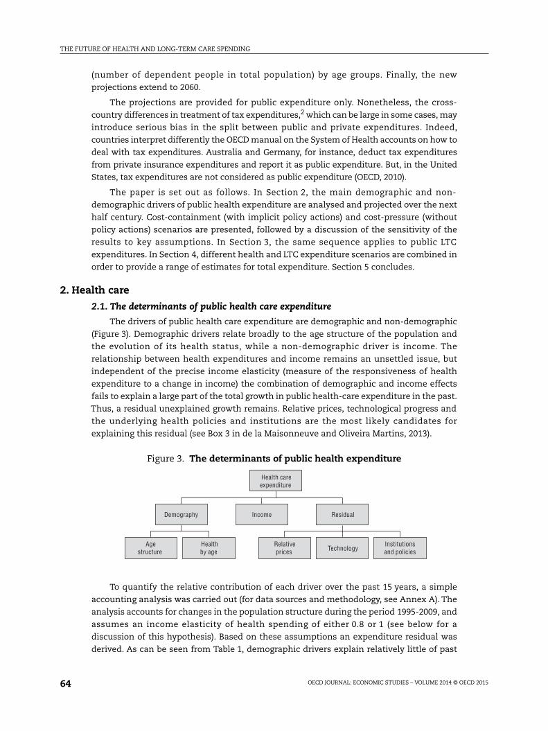
As for health care, two kinds of determinants drive LTC expenditure: demographic and

non-demographic (Figure 9). The demographic driver is related to the number of

dependent people in the population. The evolution of this factor depends on the evolution

of life expectancy and health expenditure. The non-demographic drivers are related to

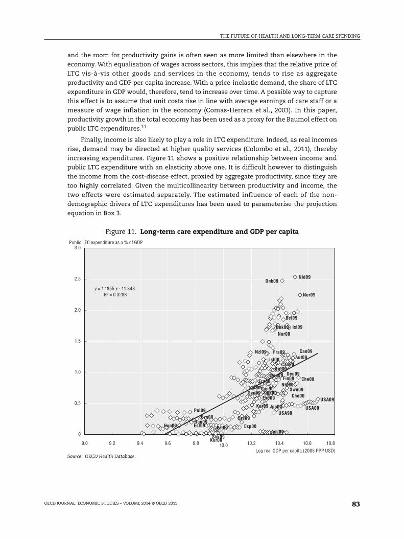
income developments and changes in the demand for public-financed LTC services.

Income is assumed to have a direct effect via increases in living standards (GDP per capita)

and an indirect effect via cost-disease (relative productivity or Baumol) effects. Given the

importance of home production of LTC services, the demand for public spending on LTC is

assumed to depend on developments in formal labour force participation.

Figure 8. Public long-term care expenditure per beneficiaryas a % of GDP per capita1

1. The graph shows the dispersion of long-term care expenditure across countries by age groups. The diamondsrepresent the median. The boxes are the 2nd and 3rd quartiles of the distribution of expenditure across countries.The whiskers are the 1st and 4th quartiles.


200

100

150

50

0


% of GDP per capita



3.1. Projection framework

The framework used to project public LTC expenditure distinguishes between

demographic and non-demographic drivers. The evolution of each driver is projected

separately. They are then combined to compute the future growth of total LTC expenditure.

The basic projection equation can be interpreted as a reduced form combining demand

and supply factors that determine equilibrium LTC expenditures. More details on these

assumptions and the corresponding variable definitions are provided below and in

Annex A. They combine a demographic effect which in the case of LTC stands for the

number of dependent people; a Baumol effect captured by the labour productivity

differential between the LTC sector and the rest of the economy with an elasticity that can

take the value of 1 or 0.5, depending on the scenario (0.5 or 0.25 for the BRIICS); an income

effect with an elasticity of LTC expenditures that can take the value of 1 or 2; and the

changes in the provision of informal care proxied by the evolution of labour force

participation of women aged 50-64 with an elasticity of 0.7.

The growth rates are first projected for each country. Applying the same methodology

as for health care, those growth rates are then adjusted to allow for a certain convergence

of LTC expenditure to GDP ratio across countries. This allows taking into account a faster

catching up of countries starting from a low basis. For instance, emerging economies such

as China or Indonesia which will face a fast growing ageing population and as a

consequence increasing demand for LTC might introduce LTC policies.

In order to smooth out the impact of the recent crisis on expenditure, the starting point for

each country is computed as the average share of public LTC spending in GDP over 2006-10. It

has to be noticed that this assumption may be too conservative. Indeed, contrary to health

care, spending has increased recently in countries where public LTC is provided.8 Public LTC is

expected to continue growing or to be introduced where it is not yet available.

3.2. Demographic drivers of expenditure

Whereas health care projections distinguished between survivors and non-survivors,

the LTC projections split each age group into dependants and non-dependants. The age-

specific dependency ratios have been estimated by the European Commission for

22 European countries (Ageing Report 2009). Even if the shape of the dependency ratios by

age differs across countries, the dispersion remains relatively limited (Figure 10). Thus, as

a first approximation, dependency ratios (number of dependants by age group) are

assumed to be broadly uniform across countries. For the purpose of projecting

Figure 9. The determinants of long-term care expenditure

Long-term areexpenditure

Demographicdrivers

Share of old-agedependants

Otherdependants

Life expectancyat birth

Health careexpenditure

Non-demographicdrivers

Income Weak

productivityInformal

care supply



expenditure, this also has the advantage of eliminating current differences in the

prevalence of dependency across countries as a possible cause for future differential

increases in LTC expenditures. In other words, the projections become less sensitive to

initial conditions. Noteworthy, this assumption therefore abstracts from the influence of

differences in policy settings on these initial conditions.

For the calculation of the pure demographic effect, it is assumed that the LTC spending

per dependant remains constant. Thus, the variation in LTC expenditure resulting from the

pure demographic effect is only driven by the increase in the number of dependants by age

group. The latter is derived from the average age-specific dependency ratio (see above)

multiplied by the population by age group.

The number of dependent people in the population depends on the evolution of

longevity and spending on health care. As the age-specific dependency ratio rises sharply

after the age of 75, any increase in life expectancy above that threshold can increase

significantly the number of old-age dependants, thereby putting pressure on LTC spending.

Moreover, as health care spending improves the probability of survival at old-age, it can

also push up LTC spending. This will be the case, for instance, if survival at older ages

translates into an increase in the prevalence of chronic diseases. However, if improvements

in life expectancy at birth translate into additional years in good health, the increase in

dependency occurs later in life. Therefore the initial spending pressures from higher

longevity are mitigated by such healthy ageing.

In order to project the evolution of dependency until 2060, taking into account the

possible link between dependency and health-care expenditures, the age-specific

dependency ratios have been estimated based on historical data as a function of age, age-

specific per capita health-care expenditures and life expectancy at birth (see Box 2).

Consistent with the healthy-ageing hypothesis, dependency at old age is found to decline

over time. But the decline of the dependency ratio by age group depends in turn on the

evolution of life expectancy at birth and per capita public health care expenditures (as

projected in the cost-containment scenario for health care).

Figure 10. Dependency ratios by age1

Number of dependants as a % of population by age groups

1. The graph shows the dispersion of the dependency ratio across countries by age groups. The diamonds representthe median. The boxes are the 2nd and 3rd quartiles of the distribution of expenditure across countries. Thewhiskers are the 1st and 4th quartiles.


80

40

60

20

0


% of age groups population



Accounting for the influence of health-care expenditure on the dependency ratio

generates a link between the health-care and LTC projections even though the two spending

items are projected separately. Clearly, this link may materialise with a lag, which is however

difficult to ascertain empirically, especially in the context of the mostly cross-section data

used in this paper. Therefore, a contemporaneous link is assumed for simplicity.

3.3. Non-demographic drivers of expenditureApart from the evolution of the number of dependants in the population, non-

demographic drivers also have an impact on LTC expenditure growth. The projections account

for three of them: changes in the relative price of LTC, income effects and changes in the

demand for public-financed LTC, which in turn depend on the availability of informal care.

One of the main non-demographic drivers of public LTC expenditure is the relative share

of informal and formal care.9, 10 Most informal care is provided by family and friends (Colombo

et al., 2011). Even using a narrow definition of the family care “workforce”, its size is at least

twice that of the formal care workforce (e.g. in Denmark), and in some cases it is estimated to

be more than ten times the size of the formal-care workforce (e.g. Canada, New Zealand, the

United States, the Netherlands). On average, around 70% to 90% of those who provide care are

family carers (Fujisawa and Colombo, 2009). Changing societal models – such as declining

family size, changes in residential patterns of people with disabilities and rising female

participation in the formal labour market – are likely to contribute to a decline in the

availability of informal care-givers, leading to an increase in the need for paid care (Colombo

et al., 2011). Since there is evidence that informal elderly care is associated with lower female

labour force participation (Viitanen, 2005), informal carers have been proxied by the labour

force participation of women aged 50-64 to project the future evolution of LTC spending (a

sensitivity check has also been carried out using their exit rate from the labour force). As

participation rates by age and gender are not readily available for non-OECD countries,

informal carers have been proxied by the overall participation rates in these countries.

Another important non-demographic driver of public LTC expenditure is a “cost

disease” or Baumol effect (Baumol, 1967; 1993). The LTC sector is highly labour-intensive

Box 2. Dependency ratio estimates

In order to gauge the evolution of the dependency ratio, its past determinants have beeninvestigated by means of panel regression techniques. Defining Depri, a as the dependencyratio (number of dependent people for country i and age a), Age as the central point in eachage bracket (2, 7, 12, …, 97), hei, a the real public health care expenditure per capita forcountry i and age a and LEi life expectancy at birth for country i, the following equation wasestimated:

The equation was estimated for the population aged 52 and above, as the dependency ratiofor people below 52 is small and roughly constant over time. As expected, the age variable hasa highly significant, positive impact (see de la Maisonneuve and Oliveira Martins, 2013). Publichealth expenditure per capita also has a significant positive effect, though much smaller.Conversely, increased life expectancy at birth delays the prevalence of dependency.

Including life expectancy at birth minimises the possibility that this effect could bedriven by health expenditures themselves, thereby avoiding multicollinearity problemsbetween health expenditure and life expectancy.

Age ( )log i,a . . .log log( ) ( )Depr ui he log LEi,a i,ai



and the room for productivity gains is often seen as more limited than elsewhere in the

economy. With equalisation of wages across sectors, this implies that the relative price of

LTC vis-à-vis other goods and services in the economy, tends to rise as aggregate

productivity and GDP per capita increase. With a price-inelastic demand, the share of LTC

expenditure in GDP would, therefore, tend to increase over time. A possible way to capture

this effect is to assume that unit costs rise in line with average earnings of care staff or a

measure of wage inflation in the economy (Comas-Herrera et al., 2003). In this paper,

productivity growth in the total economy has been used as a proxy for the Baumol effect on

public LTC expenditures.11

Finally, income is also likely to play a role in LTC expenditure. Indeed, as real incomes

rise, demand may be directed at higher quality services (Colombo et al., 2011), thereby

increasing expenditures. Figure 11 shows a positive relationship between income and

public LTC expenditure with an elasticity above one. It is difficult however to distinguish

the income from the cost-disease effect, proxied by aggregate productivity, since they are

too highly correlated. Given the multicollinearity between productivity and income, the

two effects were estimated separately. The estimated influence of each of the non-

demographic drivers of LTC expenditures has been used to parameterise the projection

equation in Box 3.

Figure 11. Long-term care expenditure and GDP per capita

Source: OECD Health Database.

3.0

2.5

1.5

1.0

2.0

0.5

0

9.0 9.2 9.4 9.6 9.8 10.0 10.2 10.4 10.6 10.8

y = 1.1855 x - 11.348 R² = 0.3288

Aus00

Aut09

Bel09

Can90

Can09

Cze09

Dnk00

Dnk09

Fra09

Deu00

Hun00

Isl09

Jpn00Kor09

Nld09

Nzl09

Nor00

Nor09

Pol09

Esp00

Esp09Swe00

Swe09Che00

Che09

USA90USA00

USA09

Aut00Can00

Fin00

Fin09Fra00

Deu09

Hun09

Isl00

Nld00

Prt00

Svk09

Svn09

Est09

Kor00

Cze00

Log real GDP per capita (2005 PPP USD)

Public LTC expenditure as a % of GDP



3.4. Projection results: Long-term care, 2010-60

As for health care, a cost-pressure scenario and a cost-containment scenario were

computed. Both scenarios are based on a unitary income elasticity assumption and the

“healthy ageing” hypothesis. However, in the cost-pressure scenario, for OECD countries, a

full Baumol effect is assumed, meaning that LTC unit labour costs increase fully in line

with aggregate labour productivity; for non-OECD countries, excess labour supply

especially in the non-tradeable sector suggests weaker wage pressures than in the OECD

countries, and therefore the cost-pressure scenario only incorporates half of the Baumol

effect. In the cost-containment scenario, the elasticity of LTC spending to productivity

increases is set at half the value of the cost-pressure scenario (0.5 for OECD countries and

0.25 for non-OECD countries), possibly reflecting policy action aimed at mitigating relative

wage increases of LTC providers. For example, action to curb expenditure could be aimed

at facilitating access to LTC provision by low-skilled migrants or at providing incentives to

balance institutional and home-based LTC.

Sensitivity analysis has been carried out in the context of the cost-containment

scenario, with respect to the Baumol effect, the income elasticity and the implications of

healthy ageing for the number of dependants. As for health care, the starting year of the

projections is an average over the period 2006-10 so as to smooth out the impact of the recent

crisis. The main assumptions underlying each projection scenario are listed in Table 6.

As with projections of public health-care spending, non-demographic drivers account

for the lion’s share of future expenditure increases (Table 7), although with an assumed

Box 3. Estimations to calibrate the LTC framework

In order to estimate the LTC spending elasticities to productivity (Baumol effect) and tothe participation rate, which are used to parameterise the projections model, the followingequation was estimated over the period 1990-2009:

where the share of long-term care expenditure in GDP [LTC/(Py*Y)] is explained by Prod, thetotal economy productivity capturing the Baumol effect (or alternatively the income percapita variable to estimate the income elasticity) and PR, the female labour forceparticipation rate used as a proxy for the provision of informal care (or alternatively theirexit rate from employment was also used). In this equation OAdep, the ratio of peopleaged 80 and above to total population, is a control variable that plays no role in theprojections, as a demographic effect already covers the effects of ageing.

As expected, the old age dependency ratio (people above 80) is a significant determinantof LTC expenditure (see de la Maisonneuve and Oliveira Martins, 2013). The relative priceeffect (proxied by total economy productivity) emerges with an elasticity of around 2.Alternatively, when the income variable is introduced, its elasticity amounts to around 2.7.While regression estimates point to Baumol or Income elasticities higher than unity, aconservative choice has been made of a unitary elasticity for both the relative price and theincome variable. Sensitivity analysis has been carried out to test for the impact of theseassumptions with the income elasticity alternatively fixed at two (see below). Finally allthe proxies for informal care (female participation or exit rate from the labour force) alsoturned out to be significant.

log * log * log * ( )LTC

P YOAdep Prod PR u

Y

log. . . .



elasticity of unity, the income effect is not creating additional pressures in terms of

expenditure shares to GDP. Demographic changes are projected to exert a relatively minor

influence on future public LTC expenditures. Indeed, as the LTC cost is independent of age,

the pure age effect has only a moderate impact on spending except where ageing is fast

enough to increase significantly the share of very-old people in the population (e.g. Korea,

China, Indonesia). Moreover, this effect is mitigated by the “healthy ageing” assumption.

3.5. The cost-pressure scenario

In the cost-pressure scenario, starting from 0.8% of GDP on average for OECD countries,

the ratio of public LTC expenditure to GDP is projected to increase by 1.4 percentage points to

reach 2.1% of GDP. However, some countries, like Chile, Estonia, Korea, Mexico and Turkey,

will experience higher increases (equal to or above 2 percentage points). These countries are

Table 6. Assumptions underlying the alternative projection scenarios: Public long-term care

Scenarios Health status Income effect Baumol effect Availability of informal care

Demographic effect Healthy ageing: The prevalenceof dependency per age is shifted

according to the evolutionof life expectancy and health

expenditure.

n.a. n.a. n.a.

Cost-pressure scenario Healthy ageing: The prevalenceof dependency per age is shifted


expenditure (cost-containmentscenario).

Income elasticity = 1 OECD countries: Full Baumoleffect (elasticity = 1).

OECD countries: Baselinescenario for participation rates

of women aged 50-64.

BRIICS: Half Baumol effect. BRIICS: Total participation rates.

Cost-containment scenario Healthy ageing: The prevalenceof dependency per age is shifted


expenditure (cost-containmentscenario).

Income elasticity = 1 OECD countries: Half Baumoleffect (elasticity = 0.5).



BRIICS: 1/4 of Baumol effect. BRIICS: Total participation rates

Sensitivity analysis based on the cost-containment scenario

Income elasticity = 2 Healthy ageing: The prevalenceof dependency per age is shifted


expenditure.




BRIICS: 1/4 of Baumol effect. BRIICS: Total participation rates.

Life expectancy plus 2 standarddeviation

Healthy ageing: The prevalenceof dependency per age is shifted

according to the evolutionof life expectancy plus2 standard deviation

and health expenditure.





Life expectancy minus2 standard deviation

Healthy ageing: The prevalenceof dependency per age is shifted

according to the evolutionof life expectancy minus

2 standard deviationand health expenditure.





Cost-pressure health scenario Healthy ageing: The prevalenceof dependency per age is shifted

according to the evolutionof life expectancy and healthexpenditure (cost pressure

scenario).





Note: The key assumption changed in each scenario is in bold.



starting from a very low level of LTC expenditure and are in the process of catching up to

higher levels. Conversely, Israel, Luxembourg, Sweden, the United Kingdom and the

United States are projected to experience only small increases in their LTC expenditure to

GDP ratios (less than 1 percentage point). Differences in the initial level of female

participation rates as well as policies in place also explain the differences across countries.

Table 7. Projection scenarios for public long-term care expenditure

Average2006-10

Percentage point deviations from starting period in 2030 Percentage point deviations from starting period in 2060

Demographiceffect

Cost-pressure

Cost-containment

Demographiceffect

Cost-pressure

Cost-containment

Australia 0.0 0.1 0.6 0.3 0.3 1.3 0.8

Austria 1.1 0.1 0.5 0.3 0.2 1.0 0.7

Belgium 1.7 0.1 0.5 0.3 0.1 1.2 0.7

Canada 1.2 0.2 0.5 0.3 0.2 1.2 0.7

Chile 0.0 0.2 0.9 0.6 0.6 2.3 1.5

Czech Republic 0.3 0.2 0.7 0.3 0.4 1.6 0.9

Denmark 2.2 0.1 0.4 0.2 0.2 1.0 0.6

Estonia 0.2 0.1 0.7 0.3 0.3 2.0 0.9

Finland 0.8 0.2 0.5 0.3 0.2 1.0 0.5

France 1.1 0.1 0.5 0.2 0.2 1.0 0.6

Germany 0.9 0.2 0.5 0.3 0.3 1.1 0.7

Greece 0.5 0.1 0.6 0.4 0.3 1.4 0.9

Hungary 0.3 0.1 0.6 0.3 0.3 1.8 1.0

Iceland 1.7 0.2 0.3 0.1 0.2 1.0 0.5

Israel 0.5 0.2 0.4 0.3 0.3 0.9 0.6

Ireland 0.4 0.1 0.5 0.4 0.2 1.0 0.7

Italy 0.7 0.1 0.5 0.3 0.2 1.2 0.8

Japan 0.7 0.2 0.5 0.3 0.3 1.4 0.8

Korea 0.3 0.4 0.8 0.5 0.8 2.0 1.3

Luxembourg 0.9 0.1 0.5 0.4 0.3 0.8 0.7

Mexico 0.0 0.2 0.7 0.5 0.6 2.2 1.5

Netherlands 2.3 0.2 0.6 0.4 0.3 1.4 0.8

New Zealand 1.3 0.2 0.5 0.3 0.3 1.4 0.8

Norway 2.1 0.1 0.4 0.2 0.2 1.0 0.5

Poland 0.4 0.2 0.7 0.3 0.5 1.8 1.0

Portugal 0.1 0.1 0.4 0.2 0.3 1.3 0.8

Slovak Republic 0.0 0.2 0.8 0.4 0.6 1.9 1.1

Slovenia 0.7 0.2 0.6 0.4 0.4 1.5 0.9

Spain 0.5 0.1 0.6 0.5 0.3 1.5 1.0

Sweden 0.7 0.1 0.4 0.1 0.1 0.9 0.5

Switzerland 1.2 0.1 0.5 0.3 0.3 1.3 0.7

Turkey 0.0 0.2 0.7 0.3 0.6 2.3 1.6

United Kingdom 0.9 0.1 0.3 0.2 0.1 0.9 0.5

United States 0.6 0.1 0.4 0.2 0.2 0.8 0.4

OECD average1 0.8 0.1 0.5 0.3 0.3 1.4 0.8

Brazil 0.0 0.2 0.3 0.3 0.7 1.2 0.9

China 0.1 0.3 0.4 0.3 0.7 2.0 1.1

India 0.1 0.1 0.3 0.2 0.4 1.5 0.8

Indonesia 0.1 0.2 0.3 0.2 0.7 1.6 1.0

Russian Federation 0.2 0.1 0.2 0.1 0.2 0.8 0.4

South Africa 0.2 0.1 0.2 0.2 0.3 0.7 0.5

Non-OECD average1 0.1 0.2 0.3 0.2 0.5 1.3 0.8

Average1 0.7 0.2 0.5 0.3 0.3 1.4 0.8

1. Unweighted average.



For non-OECD countries, the increase in LTC spending is projected to be, on average, broadly

the same as that experienced by OECD countries but starting from a much lower level (0.1%).

3.6. The cost-containment scenarioIn the cost-containment scenario, on average for OECD countries, the public LTC

expenditure to GDP ratio increases by 0.8 percentage point from 0.8% to 1.6% of GDP. Chile,

Korea, Mexico and Turkey experience the most important increases (above 1.3 percentage

points), while the increase in Finland, Iceland, Norway, Sweden, the United Kingdom and

the United States does not exceed 0.5 percentage points. Non-OECD countries will

experience on average the same increase as OECD countries (0.8 percentage points).

3.7. Sensitivity analysisGiven the uncertainty about income effects, projections were performed also

assuming an income elasticity of 2 for the cost-containment scenario for OECD countries.

For non-OECD countries, the sensitivity analysis assumed an income elasticity of 1.5. On

average, for OECD countries LTC expenditure would reach in this case 2.5% of GDP in 2060.

In this scenario, Chile, Estonia, Mexico and Turkey would experience a deviation from base

case of around 1.7 percentage points of GDP. Again, the assumptions underlying the GDP

projections assume some catch-up for these low income countries, explaining why their

LTC expenditure patterns are more affected by the higher income elasticity assumption.

For non-OECD countries, the share of LTC in GDP would reach 1.8% of GDP with the higher

income elasticity. China, India and Indonesia would experience a deviation from the base

case of more than 1 percentage point (see Table 8).

A sensitivity analysis has also been carried out for the evolution of the number of

dependants. The two drivers of the dependency ratio, life expectancy and health care

spending, have been changed separately relative to baseline. Taking life expectancy plus

(minus) two standard deviations would induce an average deviation from the base case for

OECD countries of 0.3 (-0.2) percentage points in the LTC expenditure to GDP ratio, which

would then reach, on average, 1.9% (1.4%) of GDP. For each scenario, the expenditure for

non-OECD countries will deviate from the base case by the same amount as for OECD

countries. Due to the very limited impact of health expenditure, alternative assumptions in

this area have only a slight impact. Indeed, even under the cost-pressure health care

spending scenario, the LTC expenditure to GDP ratio would only deviate from the base case

by 0.1 percentage points on average for both OECD and non-OECD countries.

4. Prospects for total public spending on healthBoth health and LTC expenditures are projected to put sizeable pressure on public

finance over the next 50 years. Overall, on average across OECD countries, the total health

and LTC expenditure to GDP ratio is projected to more than double in the cost-pressure

scenario, increasing from 6.2% in the starting period to 13.9% of GDP in 2060. In the cost-

containment scenario the ratio would still increase by more than half, to reach 9.5%

(Figure 12). For the BRIICS, starting from a much lower level, public health and LTC

expenditure will increase from 2.5% in the starting period to about 10% and above 5%

in 2060 in the cost-pressure and the cost-containment scenarios, respectively.

There are, however, striking differences across countries (Figure 13). In the cost-

containment scenario, one group of countries experiences a 4 to 5 percentage point

increase in total spending to GDP ratios over the period 2010-60. It includes countries that

are ageing very rapidly (Korea and Chile), as well as those with currently low labour force



participation especially of women, which may face a substantial increase in the demand

for formal long-term care (Spain and Mexico) as labour force participation increases and

care is no longer provided by family. By contrast, in the United States, the United Kingdom

and the Nordic countries the projected increase is below 3 percentage points of GDP. In

Table 8. Sensitivity analysis on public long-term care projectionsPerformed on the cost-containment scenario

Incomeelasticity = 21

Life expectancyplus 2 standard deviation

Life expectancyminus 2 standard deviation

Cost-pressurehealth expenditure

Percentage point deviations from cost-containment scenario in 2060

Australia 1.0 0.2 -0.2 0.1

Austria 0.6 0.2 -0.2 0.1

Belgium 0.8 0.2 -0.2 0.1

Canada 0.8 0.2 -0.2 0.1

Chile 1.7 0.3 -0.2 0.1

Czech Republic 1.3 0.3 -0.2 0.1

Denmark 0.8 0.2 -0.2 0.1

Estonia 1.8 0.3 -0.2 0.1

Finland 0.8 0.2 -0.2 0.1

France 0.6 0.2 -0.2 0.1

Germany 0.8 0.3 -0.2 0.1

Greece 0.6 0.3 -0.2 0.1

Hungary 1.4 0.3 -0.2 0.1

Iceland 0.8 0.2 -0.2 0.1

Israel 0.7 0.2 -0.2 0.1

Ireland 0.5 0.2 -0.2 0.1

Italy 0.6 0.2 -0.2 0.1

Japan 0.9 0.3 -0.2 0.1

Korea 1.0 0.4 -0.3 0.2

Luxembourg 0.1 0.3 -0.2 0.1

Mexico 1.7 0.3 -0.3 0.1

Netherlands 0.8 0.3 -0.2 0.1

New Zealand 1.2 0.2 -0.2 0.1

Norway 0.8 0.2 -0.2 0.1

Poland 1.1 0.3 -0.2 0.1

Portugal 0.7 0.3 -0.2 0.1

Slovak Republic 1.3 0.3 -0.3 0.1

Slovenia 0.9 0.3 -0.2 0.1

Spain 0.7 0.3 -0.2 0.1

Sweden 0.9 0.2 -0.2 0.1

Switzerland 0.9 0.3 -0.2 0.1

Turkey 1.7 0.3 -0.2 0.1

United Kingdom 0.8 0.2 -0.2 0.1

United States 0.7 0.2 -0.2 0.1

OECD average2 0.9 0.3 -0.2 0.1

Brazil 0.6 0.4 -0.3 0.1

China 1.2 0.4 -0.3 0.1

India 1.3 0.2 -0.2 0.1

Indonesia 1.0 0.3 -0.3 0.1

Russian Federation 0.5 0.2 -0.2 0.1

South Africa 0.7 0.2 -0.1 0.1

Non-OECD average2 0.9 0.3 -0.2 0.1

Average2 0.9 0.3 -0.2 0.1

1. Income elasticity = 1.5 for the BRIICS.2. Unweighted average.



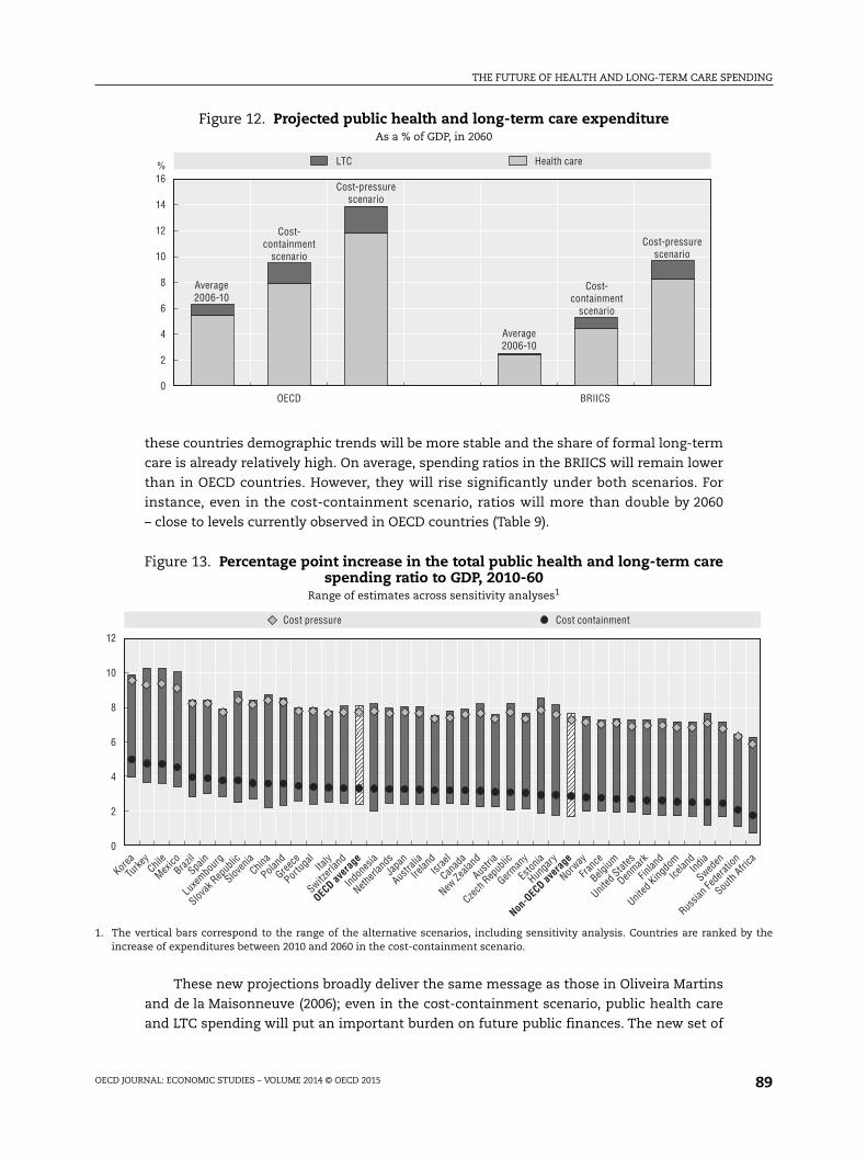
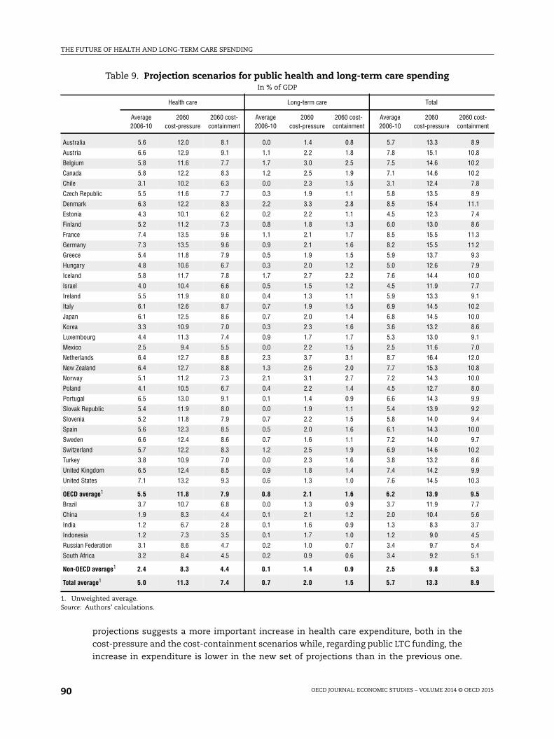
these countries demographic trends will be more stable and the share of formal long-term

care is already relatively high. On average, spending ratios in the BRIICS will remain lower

than in OECD countries. However, they will rise significantly under both scenarios. For

instance, even in the cost-containment scenario, ratios will more than double by 2060

– close to levels currently observed in OECD countries (Table 9).

These new projections broadly deliver the same message as those in Oliveira Martins

and de la Maisonneuve (2006); even in the cost-containment scenario, public health care

and LTC spending will put an important burden on future public finances. The new set of

Figure 12. Projected public health and long-term care expenditureAs a % of GDP, in 2060

16

14

12

10

8

6

4

2

0

% LTC Health care

OECD BRIICS

Average2006-10

Cost-containment

scenario

Cost-pressurescenario

Average2006-10

Cost-containment

scenario

Cost-pressurescenario

Figure 13. Percentage point increase in the total public health and long-term carespending ratio to GDP, 2010-60

Range of estimates across sensitivity analyses1

1. The vertical bars correspond to the range of the alternative scenarios, including sensitivity analysis. Countries are ranked by theincrease of expenditures between 2010 and 2060 in the cost-containment scenario.

12

10

8

6

4

2

0

Cost pressure Cost containment

Korea

Turke

yChil

e

Mexico

BrazilSpa

in

Luxe

mbour

g

Slovak

Rep

ublic

Sloven

iaChin

a

Poland

Greece

Portug

alIta

ly

Switzerl

and

OECD av

erag

e

Indon

esia

Netherl

andsJa

pan

Austra

lia

Irelan

dIsr

ael

Canad

a

New Ze

aland

Austri

a

Czech

Rep

ublic

German

y

Eston

ia

Hunga

ry

Non-O

ECD av

erag

e

Norway

Franc

e

Belgium

United

States

Denmark

Finlan

d

United

Kingdo

m

Icelan

dInd

ia

Sweden

Russia

n Fed

eratio

n

South

Africa



projections suggests a more important increase in health care expenditure, both in the

cost-pressure and the cost-containment scenarios while, regarding public LTC funding, the

increase in expenditure is lower in the new set of projections than in the previous one.

Table 9. Projection scenarios for public health and long-term care spendingIn % of GDP

Health care Long-term care Total

Average2006-10

2060cost-pressure

2060 cost-containment

Average2006-10

2060cost-pressure


Average2006-10

2060cost-pressure


Australia 5.6 12.0 8.1 0.0 1.4 0.8 5.7 13.3 8.9

Austria 6.6 12.9 9.1 1.1 2.2 1.8 7.8 15.1 10.8

Belgium 5.8 11.6 7.7 1.7 3.0 2.5 7.5 14.6 10.2

Canada 5.8 12.2 8.3 1.2 2.5 1.9 7.1 14.6 10.2

Chile 3.1 10.2 6.3 0.0 2.3 1.5 3.1 12.4 7.8

Czech Republic 5.5 11.6 7.7 0.3 1.9 1.1 5.8 13.5 8.9

Denmark 6.3 12.2 8.3 2.2 3.3 2.8 8.5 15.4 11.1

Estonia 4.3 10.1 6.2 0.2 2.2 1.1 4.5 12.3 7.4

Finland 5.2 11.2 7.3 0.8 1.8 1.3 6.0 13.0 8.6

France 7.4 13.5 9.6 1.1 2.1 1.7 8.5 15.5 11.3

Germany 7.3 13.5 9.6 0.9 2.1 1.6 8.2 15.5 11.2

Greece 5.4 11.8 7.9 0.5 1.9 1.5 5.9 13.7 9.3

Hungary 4.8 10.6 6.7 0.3 2.0 1.2 5.0 12.6 7.9

Iceland 5.8 11.7 7.8 1.7 2.7 2.2 7.6 14.4 10.0

Israel 4.0 10.4 6.6 0.5 1.5 1.2 4.5 11.9 7.7

Ireland 5.5 11.9 8.0 0.4 1.3 1.1 5.9 13.3 9.1

Italy 6.1 12.6 8.7 0.7 1.9 1.5 6.9 14.5 10.2

Japan 6.1 12.5 8.6 0.7 2.0 1.4 6.8 14.5 10.0

Korea 3.3 10.9 7.0 0.3 2.3 1.6 3.6 13.2 8.6

Luxembourg 4.4 11.3 7.4 0.9 1.7 1.7 5.3 13.0 9.1

Mexico 2.5 9.4 5.5 0.0 2.2 1.5 2.5 11.6 7.0

Netherlands 6.4 12.7 8.8 2.3 3.7 3.1 8.7 16.4 12.0

New Zealand 6.4 12.7 8.8 1.3 2.6 2.0 7.7 15.3 10.8

Norway 5.1 11.2 7.3 2.1 3.1 2.7 7.2 14.3 10.0

Poland 4.1 10.5 6.7 0.4 2.2 1.4 4.5 12.7 8.0

Portugal 6.5 13.0 9.1 0.1 1.4 0.9 6.6 14.3 9.9

Slovak Republic 5.4 11.9 8.0 0.0 1.9 1.1 5.4 13.9 9.2

Slovenia 5.2 11.8 7.9 0.7 2.2 1.5 5.8 14.0 9.4

Spain 5.6 12.3 8.5 0.5 2.0 1.6 6.1 14.3 10.0

Sweden 6.6 12.4 8.6 0.7 1.6 1.1 7.2 14.0 9.7

Switzerland 5.7 12.2 8.3 1.2 2.5 1.9 6.9 14.6 10.2

Turkey 3.8 10.9 7.0 0.0 2.3 1.6 3.8 13.2 8.6

United Kingdom 6.5 12.4 8.5 0.9 1.8 1.4 7.4 14.2 9.9

United States 7.1 13.2 9.3 0.6 1.3 1.0 7.6 14.5 10.3

OECD average1 5.5 11.8 7.9 0.8 2.1 1.6 6.2 13.9 9.5

Brazil 3.7 10.7 6.8 0.0 1.3 0.9 3.7 11.9 7.7

China 1.9 8.3 4.4 0.1 2.1 1.2 2.0 10.4 5.6

India 1.2 6.7 2.8 0.1 1.6 0.9 1.3 8.3 3.7

Indonesia 1.2 7.3 3.5 0.1 1.7 1.0 1.2 9.0 4.5

Russian Federation 3.1 8.6 4.7 0.2 1.0 0.7 3.4 9.7 5.4

South Africa 3.2 8.4 4.5 0.2 0.9 0.6 3.4 9.2 5.1

Non-OECD average1 2.4 8.3 4.4 0.1 1.4 0.9 2.5 9.8 5.3

Total average1 5.0 11.3 7.4 0.7 2.0 1.5 5.7 13.3 8.9

1. Unweighted average.Source: Authors’ calculations.



Overall, on average, the current projections suggest only a slightly lower increase in total

health and LTC expenditure confirming the message delivered by the previous set of

projections. A comparison between these new projections and the ones from the European

Commission, the IMF and the Congressional Budget Office in the United States suggests that

the differences arise mainly as a consequence of varying assumptions concerning the future

evolution of the main drivers of spending (see de la Maisonneuve and Oliveira Martins,

2013 for details). The EC projected increases in health-care expenditure are the lowest due to

the nearly unitary income elasticity associated with the absence of a residual growth. The

IMF projections, although difficult to compare as they end in 2050, seem to range between

the OECD cost-containment and cost-pressure scenarios. The assumption of low income

elasticity is broadly offset by the country specific residual. Nonetheless when the estimated

residual is higher than the average like in the United States, the projected increase in health

care expenditure is much higher. This high increase is corroborated by the CBO projections.

5. Concluding remarksLong-term spending projections are inherently uncertain and subject to upside or

downside risks. While a more moderate evolution of spending than in these projections

cannot be excluded (for instance if cost-saving technologies were to spread out, or if more

aggressive cost-containment policies were to be implemented), there are also clear upside

risks on spending. For instance, higher health spending could arise due to an extension of

the pre-death period of ill health as longevity increases, or because of higher than expected

costs induced by technical progress. Regarding LTC, higher spending could arise from

increased dependency due to obesity trends or dementia. Indeed, according to recent

calculations, some 12% of those aged between 80 and 84 years, and almost one in four of

those aged over 85 years, suffer from dementia (Alzheimer Europe, 2006). With ageing

populations, strong increases in the prevalence of dementia may be expected (see Box 1.1

in Colombo et al., 2011), though prevention and treatment may also improve in the future.

Even if these upside risks do not materialise, the spending projections point to

important policy challenges. These challenges are reinforced by the evidence that

macroeconomic cost-containment policies, which had some success in repressing

spending trends over the 1980s and 1990s, have their limits. For instance, it is difficult to

contain wages and at the same time, attract young and skilled workers into the health-care

system. Similarly, controlling prices is not easy when technical progress is permanently

creating new products and treatments, while overall constraints on supply result in

unpopular waiting lists for these treatments. More generally, it is difficult to determine the

appropriate supply of health and LTC services without market signals – but at the same

time, health and LTC are areas where market failure is rife.

Notes

1. To focus on the structural factors and eliminate cyclical effects, the ratio is computed using trendinstead of actual GDP (from the OECD Economic Outlook, No. 91).

2. Tax expenditure can be of different kinds, e.g. exclusion from workers’ taxable income ofemployers’ health insurance contributions in the United States, tax credits for medical expensesin Canada or income tax deductions for health care services in Portugal.

3. For more details, see Johansson et al. (2012).



4. While the probability of dying increases with age, the costs of death tend to decline steadily afteryoung and prime age (Aprile, 2004). Other estimates of DRC are coherent with this order ofmagnitude (e.g. Yang et al., 2003).

5. See, for example Fuchs (1984); Zweifel et al. (1999); Jacobzone (2003); and Gray (2004).

6. While he/N and Y/N are found to be I (1) and co-integrated, the complete VECM with all explanatoryvariables did not provide good results. Thus a regression on growth rates addresses the problem ofa possible spurious correlation between the two variables. The results presented in the last columnof Table 2 confirm the level estimates.

7. It has to be noted that depending on the type of expenditure this upward shift may be non-homothetic across ages. For example, expenditure at older ages may be more affected by such anupward shift than at younger ones.

8. For instance, Korea introduced the public LTC insurance in 2008 and it has increased since then.The same occurred in Estonia, Japan and Portugal.

9. Formal care is provided by care assistants who are paid for providing care under some form ofemployment contract. It includes both care provided in institutions and care provided at home. Tobe considered informal, the provision of care cannot be paid for as if purchasing a service.However, an informal care-giver may still receive social transfers conditional on his/her provisionof informal care and possibly, in practice, some informal payment from the person receiving care.

10. The projections do not distinguish between formal care delivered within institutions and thatdelivered to the patient’s home. There are fundamental differences between countries in the waythey organise their formal LTC. Institutional LTC is particularly widespread in the Nordic countries(OECD, 2005). Whether this form of organisation is adopted by other countries or a (cheaper)ambulatory help-at-home strategy is pursued could have important consequences for publicexpenditures.

11. The relative price effect may be limited by a growing share of immigrants among LTC workers.According to Colombo et al., (2011), foreign-born workers play a significant and growing role in LTCin some countries. The average wage of the immigrant work force is lower than that of nativeworkers and their bargaining power is weaker. The process of equalising the wages of foreign-bornand native work forces will take time, but will certainly materialise over the long run.

References

Acemoglu, D., A. Finkelstein and M. Notowidigdo (2009), “Income and Health Spending: Evidence fromOil Shocks”, CEPR Discussion Papers, No. 7255.

Alzheimer Europe (2006), Dementia in Europe Yearbook 2006, Luxembourg.

Aprile, R. (2004), “How to Take Account of Death-Related Costs in Projecting Health Care Expenditure– Updated Version”, Ragioneria Generale Dello Stato.

Baumol, W.J. (1967), “Macroeconomics of Unbalanced Growth: The Anatomy of Urban Crisis”, AmericanEconomic Review, 57, pp. 415-426.

Baumol, W.J. (1993), “Health Care, Education and the Cost of Disease: A Looming Crisis for PublicChoice,” Public Choice, 77, pp. 17-28.

Bessen, J. and T. Grid (2013), “Which Patent Systems Are Better For Inventors?”.

Breyer, F. and S. Felder (2006), “Life Expectancy and Health Care Expenditures: A New Calculation forGermany Using the Costs of Dying”, Health Policy, 75, pp. 178-186.

Breyer, F, J. Costa-i-Font and S. Felder (2011), “Does Ageing Really Affect Health Expenditures? If So,Why?”, Vox EU, May.

Burniaux, J.M., R. Duval and F. Jaumotte (2003), “Coping with Ageing: A Dynamic Approach to Quantifythe Impact of Alternative Policy Options on Future Labour Supply in OECD Countries”, OECDEconomics Department Working Papers, No. 371, OECD Publishing.

Colombo, F. et al., (2011), “Help Wanted? Providing and Paying for Long-Term Care”, OECD Health PolicyStudies, OECD Publishing.

Comas-Herrera and R. Wittenberg (eds.) (2003), European Study of Long-Term Care Expenditure:Investigating the Sensitivity of Projections of Future Long-Term Care Expenditure in Germany, Spain, Italyand the United Kingdom to Changes in Assumptions About Demography, Dependency, Informal Care, FormalCare and Unit Costs, PSSRU, LSE Health and Social Care, London School of Economics.



Congressional Budget Office (2012), The 2012 Long-Term Budget Outlook.

De la Maisonneuve, C. and J. Oliveira Martins (2013), “A Projection Method for Public Health and Long-Term Care Expenditures”, OECD Economics Department Working Papers, No. 1048.

European Commission, 2009 Ageing Report: Economic and Budgetary Projections for the EU27 Member States(2008-60).

Felder, S., M. Meier and H. Schmitt (2000), “Health Care Expenditure in the Last Months of Life”, Journalof Health Economics, 19, pp. 679-95.

Fuchs, V. (1984), “’Though Much is Taken’ – Reflections on Ageing, Health and Medical Care”, NBERWorking Paper, No. 1269.

Fujisawa, R. and F. Colombo (2009), “The Long-Term Care Workforce: Overview and Strategies to AdaptSupply to a Growing Demand”, OECD Health Working Paper, No. 44, OECD Publishing.

Getzen, T. (2000), “Health Care is an Individual Necessity and a National Luxury: Applying MultilevelDecision Models to the Analysis of Health Care Expenditure”, Journal of Health Economics, 19,pp. 259-270.

Gray, A. (2004), “Estimating the Impact of Ageing Populations on Future Health Expenditures”, Publiclecture to the National Institute of Economics and Business and the National Institute of Healthand Human Science, 4 November, Canberra.

Holly, A., X. Ke and P. Saksena (2011), “The Determinants of Health Expenditure: A Country-Level PanelData Analysis”, World Health Organisation Working Paper.

International Monetary Fund (2012), “The Economics of Public Health Care Reform in Advanced andEmerging Economies”.

Jacobzone, S. (2003), “Ageing and the Challenges of New Technologies: Can OECD Social and HealthCare Systems Provide for the Future?”, The Geneva Papers on Risk and Insurance, Vol. 28, No. 2, April,pp. 254-74.

Johansson, A. et al. (2012), “Long-Term Growth Scenarios”, OECD Economics Department Working Papers,No. 1000, OECD Publishing.

OECD (2005), Long-Term Care for Older People, OECD Publishing.

OECD (2006), “Projecting OECD Health and Long-Term Care Expenditures: What are the Main Drivers?”,OECD Economics Department Working Papers, No. 477, OECD Publishing.

OECD (2010), Health Care Systems: Efficiency and Policy Settings, OECD Publishing.

OECD (2011), Health Data, OECD Publishing.

OECD (2012), OECD Economic Outlook, Vol. 2012/1, OECD Publishing.

OECD (2013), Health Data, OECD Publishing.

Okunade, A.A. and V.N.R. Murthy (2002), “Technology as a Major Driver of Health Costs:A Cointegration Analysis of the Newhouse Conjecture”, Journal of Health Economics, 21, pp. 147-159.

Oliveira Martins, J. and C. de la Maisonneuve (2006), “The Drivers of Public Expenditure on Health andLong-Term Care: An Integrated Approach”, OECD Economic Studies, No. 43, 2006/2.

Seshamani, M. and A. Gray (2004), “A Longitudinal Study of the Effects of Age and Time to Death onHospital Costs”, Journal of Health Economics, 23, pp. 217-35.

Viitanen, T.K. (2005), “Informal Elderly Care and Female Labour Force Participation Across Europe”,Center for European Policy Studies, ENEPRI Research Reports, No. 13, 1, July.

Werblow, A., S. Felder and P. Zweifel (2007), “Population Ageing and Health Care Expenditure: A Schoolof ’Red Herrings’?”, Health Economics, 16, pp. 1109-26.

Yang, Z., E.C. Norton and S.C. Stearns (2003), “Longevity and Health Care Expenditures: The RealReasons Older People Spend More”, Journal of Gerontology, Vol. 58B, No. 1, pp. S2-S10.

Zweifel, P., S. Felder and M. Meiers (1999), “Ageing Of Population And Health Care Expenditure: A RedHerring?”, Health Economics, 8, pp. 485-496.



ANNEX A

Data sources and method

Health and LTC data

Health and LTC expenditures

The historical public current health and LTC expenditure to GDP ratios come from the

OECD Health Database (2011) that provides comparable health statistics across OECD

countries. Total public current expenditure on health is the sum of total personal and total

collective services but excludes investment. The LTC spending corresponds to the “Services

of long-term nursing care” item. The latter is subtracted from the Total public current

expenditure to get the health spending.

Total expenditure on health is defined as the sum of expenditure on activities that

– through application of medical, paramedical, and nursing knowledge and technology –

are aimed at: promoting health and preventing disease; curing illness and reducing

premature mortality; caring for persons affected by chronic illness who require nursing

care; caring for persons with health-related impairments, disability, and handicaps who

require nursing care; assisting patients to die with dignity; providing and administering

public health; providing and administering health programmes, health insurance and

other funding arrangements. Public expenditure on health care is health expenditure

incurred by public funds. Public funds are state, regional and local Government bodies and

social security schemes.

Long-term health care comprises ongoing health and nursing care given to in-patients

who need assistance on a continuing basis due to chronic impairments and a reduced

degree of independence in activities of daily living. In-patient long-term care is provided in

institutions or community facilities. Long-term care is typically a mix of medical (including

nursing care) and social services.

Cost curves by age groups

The public health expenditure by age groups have been provided by the European

Commission for the European countries (2009 Ageing Report) and by the Swiss Federal

Statistical Office, Health Canada and the Australian Institute for Health and Welfare for

Switzerland, Canada and Australia, respectively. These cost curves are split into survivors

and non-survivors as explained in the text.



An average expenditure curve for survivors was estimated econometrically in a panel

of 23 countries and 20 age groups, using a spline function as follows:

where he is the real health expenditure by age group, N population by age group and age is

the central point in each bracket (e.g. 2, 7, 12, …, 97).

For each country, this expenditure curve by age group is multiplied by country-specific

population by age group in order to obtain a total country-specific health expenditure. This

expenditure is then calibrated to fit with the OECD database total expenditure in the base year.

LTC Dependency ratios

The dependency ratios (number of dependants by age group) were derived from the

European Commission 2009 Ageing Report. Even if the shape of the dependency ratios by

age differs across countries, the dispersion remains relatively limited (Figure 10 in the

main text). Accordingly, dependency ratios are assumed to be broadly uniform across

countries and an average dependency ratio by age group was calculated and used in the

projections. The dependency ratios are then projected using the evolution of life

expectancy at birth and health expenditure (cost-containment scenario). The life

expectancies at birth are those underlying official population projections.

Macro data

GDP

GDP projections are published in the OECD Economic Outlook, No. 91. More details

regarding the sources and the methodology can be found in Johansson et al. (2012). In

short, GDP projections are based on a conditional convergence model.

Population

Population projections come from Eurostat for European Countries (EUROPOP2010)

and from the United Nations for non-European Countries (World Population Prospects: The

2010 Revision).

Health prices and technology

The health price measure used in this paper is the value-added deflator in the health

and social work sectors, taken from the OECD STAN Database. Even if this measure may not

be as accurate as needed, it is nonetheless more comparable across countries than more

precise price indicators available from other sources. For instance, CPI series for the health

sector can be gathered from Eurostat (for European countries) and national sources (for

Australia, Canada, Korea, New Zealand and the United States). The CPI series cannot,

however, be used because they are available for too short a period (the HICP from Eurostat

is only available from 1996 onwards) and there is also a potential lack of comparability

across countries.

The quality effect combines an indicator of patents with an indicator of R&D statistics.

The patents granted by the European Patent Office (EPO) have been chosen as they seem to

generate substantially greater market power than their US equivalents (Bessen, 2013) and

may represent the OECD-wide technology frontier (see de la Maisonneuve and

he

Nage age ageage group

age group. . . . . . . 199 1 14 5 0 41 0 0052 3 .. . .age age4 50 00002



Oliveira Martins, 2013). They come from the OECD database on Patents. To benefit from

advances in this frontier, countries need to innovate and absorb foreign technology (via

technology pass-through and catching up effects). While not all R&D expenditures are

medical, they may advance health care technology because of externalities (Okunade and

Murthy, 2002); moreover, high R&D spending is needed to enable the adoption of foreign

technologies (the so-called absorption potential). Hence, the ratio of total R&D expenditure

to GDP has been used as a proxy for the ability of a country to reach the frontier. The data

come from the OECD R&D database.

Baumol effect

The “cost-disease” Baumol effect is proxied by the productivity growth in total

economy. The productivity data come from the OECD Economic Outlook, No. 91, and

Johansson et al. (2012). It is calculated as real GDP per worker in 2005 constant PPP USD.

Participation rate

Participation rates are those underlying GDP projections and come from the OECD

Economic Outlook, No. 91, and Johansson et al. (2012). For OECD countries, the participation

rate projections are based on the so-called “cohort approach” (Burniaux et al., 2003). The

cohort approach assumes that the observed participation behaviour of individuals

belonging to the most recent cohorts, such as the lower exit rates of current old-age

workers relative to previous cohorts, or the higher entry rates of current young women

relative to previous cohorts, will continue to apply to future cohorts as well. Therefore,

future participation rates are determined by the participation behaviour of the most recent

cohorts and the evolution of the relative weight of different cohorts, which is driven by

demographic developments (see Johansson et al., 2012, for more details).

Some policy reforms are taken into account in the labour force participation projections.

First, the long-term trend expansion in education – and the associated increase in average

years of schooling – is assumed to continue in all countries. Second, longer life expectancy

and health improvements raise the scope for policies that encourage higher labour market

participation at older age. And finally, a number of countries have already implemented or

plan to implement reforms aiming to extend working lives, including by increasing the

legal age to get a full pension. Recently-legislated pension reforms that involve an increase

in the normal retirement age by 2020 are assumed to be implemented as planned* (see

Johansson et al., 2012, for more details).

* The countries for which an adjustment on current exit rates of older workers are made includeAustralia, Belgium, Canada, Czech Republic, Germany, Spain, Estonia, France, the United Kingdom,Greece, Hungary, Ireland, Israel, Italy, Japan, New Zealand, Slovak Republic, Slovenia, Turkey andthe United States.

Date post:	05-Jun-2018
Category:	Documents
Upload:	dinhnguyet
View:	213 times
Download:	0 times

The future of health and long-term care spending - OECD.org · OECD Journal: Economic Studies...

Documents