Page 1
THE GAP BETWEEN NECESSITY AND SUFFICIENCY FOR
STABILITY OF SPARSE MATRIX SYSTEMS: SIMULATION STUDIES
BY
TAO YANG
THESIS
Submitted in partial fulfillment of the requirements for the degree of Master of Science in Electrical and Computer Engineering
in the Graduate College of the University of Illinois at Urbana-Champaign, 2015
Urbana, Illinois
Adviser:
Assistant Professor Mohamed Ali Belabbas
Page 2
ii
Abstract
Sparse matrix systems (SMSs) are potentially very useful for graph analysis and topological
representations of interaction and communication among elements within a system. Such systems’
stability can be determined by the Routh-Hurwitz criterion. However, simply using the Routh-Hurwitz
criterion is not efficient in this kind of system. Therefore, a necessary condition can save a lot of work.
The necessary condition is of importance and will be discussed in this thesis. Also, meeting the necessary
condition does not mean it is safe to claim the SMS is stable. Therefore, another part of this project is to
see how effective the necessary condition is by simulations. The simulation shows that approximate
SMSs meeting the necessary condition are very likely to be stable. The results approach 90-95%
effectiveness given enough trials.
Page 3
iii
Acknowledgments
I appreciate my professors, classmates and friends including Shuo Li, Mujing Wang, Xiang Zhao,
Aiyin Liu, Tian Xia, Moyang Li, Shu Chen, Yuhao Zhou and Guosong Yang for their help and support
during these years in the ECE department at the University of Illinois at Urbana-Champaign. I also thank
my parents and my girlfriend for the unceasing encouragement, support and attention. Lastly, I am
grateful to my academic advisor, Professor Belabbas, for his supervision and teaching in ECE 486, ECE
598 and ECE 555, in which I learned important skills for my future career development.
Page 4
iv
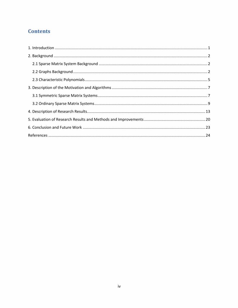
Contents
1. Introduction .............................................................................................................................................. 1
2. Background ............................................................................................................................................... 2
2.1 Sparse Matrix System Background ..................................................................................................... 2
2.2 Graphs Background ............................................................................................................................. 2
2.3 Characteristic Polynomials .................................................................................................................. 5
3. Description of the Motivation and Algorithms ......................................................................................... 7
3.1 Symmetric Sparse Matrix Systems ...................................................................................................... 7
3.2 Ordinary Sparse Matrix Systems ......................................................................................................... 9
4. Description of Research Results .............................................................................................................. 13
5. Evaluation of Research Results and Methods and Improvements ......................................................... 20
6. Conclusion and Future Work .................................................................................................................. 23
References .................................................................................................................................................. 24
Page 5
1
1. Introduction
The Network topology is widely utilized in social networks, search engines, communication
models and control. Starting from the beginning of the twentieth century, our knowledge of what can
model the network has been pushed forward greatly. Starting from the Watts-Strogatz model [1] to the
Barabási–Albert Scale-Free model [2], researchers have studied problems in this field for decades. To find
the existence of stability of network topology, research on graph theory problems always includes
network topology describing interactions within a system. See for examples [3]-[9].
The stability of linear systems is well defined and researched by the Routh-Hurwitz criterion [10],
so there is no need to discuss it. But for sparse matrix systems, which will be discussed in the background
section, checking eigenvalues is not the best option. Therefore, we propose a necessary condition which
can guarantee almost all matrices to be stable. To determine how effective the necessary condition is, we
have done several simulations and found the conditional probability of stable matrices generated
randomly in sparse matrix spaces, given they meet the necessary condition.
The theis is structured as follows. In chapter 2, we will give a brief discussion of sparse matrix
systems, graphs and characteristic polynomials, which are of essential importance in the simulations.
Chapter 2 also provides a literature review with theoretical analysis and formal definitions on sparse
matrix systems. In Chapters 3 and 4, we will present the motivations, algorithms and results for the
simulations. Chapter 5 offers evaluations and discussions on different methods we take advantage of in
the simulation, and Chapter 6 is the conclusion.
Page 6
2
2. Background
2.1 Sparse Matrix System Background
A sparse matrix system (SMS) is a vector space in which entries can be either arbitrary real number
or zero [11]. Let n > 0 be the dimension of a square matrix, and α is a set of pairs of integers between 1
and n; that means α ⊂ {1, . . . , n} × {1, . . . , n}. Eij denotes the n × n matrix with non-zero ij entry, and all
other entries are zero.
As a result, we can define Σα as a vector space of matrices with the form of
𝐴 = Σ(𝑖,𝑗)⊂α𝑎𝑖𝑗𝐸𝑖𝑗 , 𝑎𝑖𝑗 ∈ 𝑅
For example, consider a space with n=2, and α = {(1, 2), (2, 1), (2, 2)}. A is the subspace of matrices of
the form
𝐴 = [0 ∗∗ ∗
]
And * are arbitrary real numbers.
Given a SMS Σ, the non-zero entries are free variables, and the entries denoted by * can be
arbitrary values. Thus, to test the stability by the Routh-Hurwitz criterion can be tiresome because each
time one unique matrix is sampled in accordance with the given SMS, we need to apply the criterion again.
Though the stability of such matrices is clear by applying the criterion, it is very hard to test the stability
of millions of sampled matrices under the SMS subspace.
2.2 Graphs Background
Let us start with some definitions. A graph is an ordered pair G=(V,E). V is the vertex set whose
elements are the vertices, or nodes of the graph. And the set is often denoted V(G) or V. E is the edge set
whose elements being the edges, or connections between vertices, of the graph. This set is often denoted
E(G ) or E. If the graph is undirected, individual edges are unordered pairs {u, v} with u and v being vertices
in V. If the graph is directed, edges are ordered pairs (u, v). Nodes in the graph may be connected by
Page 7
3
single edges or multi-edges, which means there are more than one edge between the same pair of
vertices. A loop exists when an edge connects a vertex to itself. The simple graph is a graph in which there
are no self-edges and multi-edges.
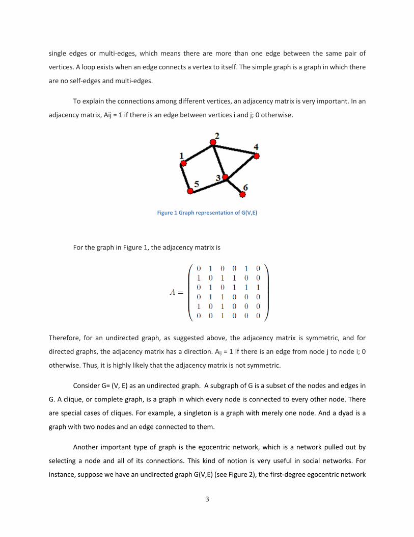
To explain the connections among different vertices, an adjacency matrix is very important. In an
adjacency matrix, Aij = 1 if there is an edge between vertices i and j; 0 otherwise.
Figure 1 Graph representation of G(V,E)
For the graph in Figure 1, the adjacency matrix is
Therefore, for an undirected graph, as suggested above, the adjacency matrix is symmetric, and for
directed graphs, the adjacency matrix has a direction. Aij = 1 if there is an edge from node j to node i; 0
otherwise. Thus, it is highly likely that the adjacency matrix is not symmetric.
Consider G= (V, E) as an undirected graph. A subgraph of G is a subset of the nodes and edges in
G. A clique, or complete graph, is a graph in which every node is connected to every other node. There
are special cases of cliques. For example, a singleton is a graph with merely one node. And a dyad is a
graph with two nodes and an edge connected to them.
Another important type of graph is the egocentric network, which is a network pulled out by
selecting a node and all of its connections. This kind of notion is very useful in social networks. For
instance, suppose we have an undirected graph G(V,E) (see Figure 2), the first-degree egocentric network
Page 8
4
of a node A is composed with the edges stretched out from A and the nodes connected to A. Also, there
is a so-called 1.5-degree egocentric network of A, which includes the edges connected to neighbors of A
and the 1-degree egocentric network of A. A 2-degree egocentric network further includes the neighbors
of neighbors of A.
Figure 2 Example of egocentric graph. The 1-degree egocentric network of A includes edges marked by red and A’s neighbors. 1.5-degree egocentric network of A includes 1-degree network plus the blue edges. Black edges, nodes connected by those
edges and 1.5-degree egocentric network are included in the 2-degree network of A.
For an undirected network, the degree of a vertex or node is
𝑑(𝑣𝑖) = |𝑣𝑗| 𝑠. 𝑡. 𝑒𝑖𝑗 ∈ 𝐸 ∧ 𝑒𝑖𝑗 = 𝑒𝑗𝑖
For a directed network, the degree of a node needs to be discussed in two directions. For an edge
pointing inward to a node, we denote it as 𝑑𝑖𝑛(𝑣𝑖); and we denote outward edges as 𝑑𝑜𝑢𝑡(𝑣𝑖). 𝑑𝑖𝑛(𝑣𝑖)
is the number of edges pointing to 𝑣𝑖, whereas 𝑑𝑜𝑢𝑡(𝑣𝑖) is the number of edges 𝑣𝑖 . The formal definitions
of 𝑑𝑖𝑛(𝑣𝑖) and 𝑑𝑜𝑢𝑡(𝑣𝑖) are as follows.
𝑑𝑖𝑛(𝑣𝑖) = |𝑣𝑗| 𝑠. 𝑡. 𝑒𝑖𝑗 ∈ 𝐸
𝑑𝑜𝑢𝑡(𝑣𝑖) = |𝑣𝑗| 𝑠. 𝑡. 𝑒𝑗𝑖 ∈ 𝐸
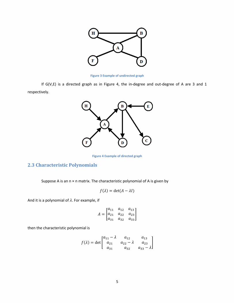
For example, for the undirected graph in Figure 3, the degrees of node A and Node B are 4 and 3
respectively.
Page 9
5
Figure 3 Example of undirected graph
If G(V,E) is a directed graph as in Figure 4, the in-degree and out-degree of A are 3 and 1
respectively.
Figure 4 Example of directed graph
2.3 Characteristic Polynomials
Suppose A is an n × n matrix. The characteristic polynomial of A is given by
𝑓(𝜆) = det (𝐴 − 𝜆𝐼)
And it is a polynomial of 𝜆. For example, if
𝐴 = [
𝑎11 𝑎12 𝑎13
𝑎21 𝑎22 𝑎23
𝑎31 𝑎32 𝑎33
]
then the characteristic polynomial is
𝑓(𝜆) = det [
𝑎11 − 𝜆 𝑎12 𝑎13
𝑎21 𝑎22 − 𝜆 𝑎23
𝑎31 𝑎32 𝑎33 − 𝜆]
Page 10
6
𝑓(𝜆) = 𝜆3 − (𝑎11 + 𝑎22 + 𝑎33)𝜆2 + (𝑎11 × 𝑎22 − 𝑎12 × 𝑎21 + 𝑎11 × 𝑎33 − 𝑎13 × 𝑎31+𝑎33 × 𝑎22 −
𝑎23 × 𝑎43)𝜆 − 𝑎11 × 𝑎22 × 𝑎33 + 𝑎11 × 𝑎23 × 𝑎32 + 𝑎12 × 𝑎21 × 𝑎33 − 𝑎12 × 𝑎23 × 𝑎31 −
𝑎13 × 𝑎21 × 𝑎32 + 𝑎13 × 𝑎22 × 𝑎31
Here we can find that the coefficient of the second highest order term is the trace multiplied by
-1. Most of the simulation will be around the coefficients of the polynomials. However, if the dimension
of the matrix gets very large, the characteristic polynomials will be very complicated since for larger
matrices, the determinants are difficult to solve. The determinant of A, given A is an n × n matrix, depends
on the (n-1) × (n-1) matrix it contains, as we all know. Therefore, if any column index j is fixed, the
mathematical expression for the determinant of A is
𝑑𝑒𝑡 𝐴 = 𝛴𝑖=1𝑛 (−1)𝑖+𝑗𝐴𝑖𝑗 𝑑𝑒𝑡 𝐴(𝑖|𝑗)
Usually, (−1)𝑖+𝑗 det 𝐴(𝑖|𝑗) is referred as the 𝑖, 𝑗 cofactor of A. And if we define
𝐶𝑖𝑗 = (−1)𝑖+𝑗𝑑𝑒𝑡 𝐴(𝑖|𝑗)
Then for each j,
𝑑𝑒𝑡 𝐴 = 𝛴𝑖=1𝑛 𝐴𝑖𝑗𝐶𝑖𝑗
Therefore, for larger square matrices, the characteristic polynomials are very difficult to solve because we
need to iteratively compute the determinants to the end; thus, we decide to let the computer compute
the numerical values of coefficients of polynomials when dimensions are large.
Page 11
7
3. Description of the Motivation and Algorithms
3.1 Symmetric Sparse Matrix Systems
As suggested above, the necessary condition is not able to guarantee that the sparse matrix
system is stable. However, for symmetric matrices, the necessary condition and the Routh-Hurwitz
criterion are equivalent.
The algorithm to build a symmetric matrix is quite special because there are constraints on the
number of zeros and the dimension of the matrix. The first step is to set up a matrix with all values of
entries drawn from the standard normal distribution. Then, knowing the number of zeros in the matrix,
initially we plan to assign zeros in random entries which are symmetric two by two. Soon, after several
testing cases, we find the assignments are very strange, since if the random position picked by the
computer is a diagonal entry, the next assignment of zero will be at the same place. As a result, even
though the computer records that it has finished two assignments of zeros randomly, in fact, there would
be only one zero which has been assigned. In this case, after finishing the random assignments of zeros,
the number of zeros in this symmetric sparse matrix system is less than or equal to the planned number
of zeros. In this process, the mistakes we made included the repetition of assignments of the same non-
diagonal positions and missed assignments in diagonal entries.
To revise the algorithm, we consider what cases we should be aware of to prevent the missed
assignments. At last, we conclude that several cases are dangerous to this simulation. First, if the number
of zeros in this sparse matrix system is odd, there also will be an odd number of diagonal entries which
are zero. After a certain number of assignments, if there are no spaces for zeros in diagonal entries and
the number of zeros needed to be assigned is odd, this configuration of symmetric sparse matrix system
will fail. Second, if there is only one available space for the assignments, the program needs to avoid the
assignments in that spot if the remaining zeros are even.
The pseudocode for setting up symmetric sparse matrix system as follows:
Pseudocode for Setting Up Symmetric Sparse Matrix Systems
<n :the number of zeros planned in matrix>
<j :the number of zeros assigned already >
START
Page 12
8
Declare A with all entries drawn from standard normal distribution;
Mark all diagonal entries of A as available;
j=0;
WHILE(j < n)
Get random entry coordinate (i, j);
IF(n = 1)
Assign zero at random diagonal entry;
j=j+1;
ELSE
IF(n – j > 1)
IF(A(i, j) ≠ 0)
A(i, j) = 0;
j=j+1;
IF(i ≠ j)
A(j, i) = 0;
ELSE
Mark this diagonal entry A(i, i) has been taken;
ELSE
IF(There are still available spaces of diagonal entries)
Get random available entry A(k,k);
A(k,k) = 0;
j = j+1;
ELSE
Redo the configuration of symmetric sparse matrix system
STOP
Keeping these two special cases in mind, we revise the code by adopting a fail-safe mechanism. If
there is only one zero that needs to be assigned, the only spaces which can be assigned are diagonal
entries because they are at the axis of the symmetry. Otherwise, if more than one zero needs to be
assigned, it is safe to pick any position, but we need to mark the availability of diagonal entries. The worst
case is that there is no space in diagonal entries when there is still one zero that needs to be assigned. In
that case, we decide to let the program redo this configuration.
After the configuration, other procedures look much nicer: we simply apply the necessary
condition and Routh-Hurwitz criterion and check the probabilities. The probabilities given by both
methods look exactly the same. Also, using determinants of the matrix is an alternative and they are all
equivalent.
Page 13
9
3.2 Ordinary Sparse Matrix Systems
Unlike the symmetric matrix, the arbitrary sparse matrix system form is easier to set up. However,
we decided to change some inputs of the simulation to make it more convenient. Therefore, we stop using
the number of zeros in sparse matrix system; instead, we determine the number of zeros by setting a
probability for an entry to be zero. In Matlab, the rand() function returns a random number between 0
and 1. If the returned value is above the threshold we set, the entry we are assigning this time will be
zero. By setting up the threshold, we can determine the expected number of zeros in an n-dimensional
sparse matrix system. After multiple simulations, we find the difference between the necessary condition
and the Routh-Hurwitz criterion.
We utilized three methods in the research to generate random numbers. First, we used the
method of drawing the number from standard normal distribution, and the numbers of entries drawn
from standard normal distribution lead to very low probability of meeting the Routh-Hurwitz criterion.
The reason is that the possibility of retrieving a positive number is quite high. Therefore, potentially we
have to try more iterations to check whether there is at least one matrix in sparse matrix space that is
stable. To improve the efficiency of the iterations and expedite the calculations, we decided to shift the
normal distribution to the negative direction a little bit. We simply subtract the number drawn from the
standard normal distribution shifted left by 0.1 (N(-0,1, 1)). The result seems to be more efficient and the
running time is less. However, the probability of picking numbers from negative infinity to positive infinity
is not the same due to the nature of Gaussian distribution. But to have all numbers with the same
probability to be picked, we used the function of inverse of normal distribution with mean of 0 and
standard deviation of 1 to generate a random number from negative infinity to positive infinity.
The algorithm mainly contains two parts; the first part consists of the iterations to see whether a
sparse matrix system meets the necessary condition and the Routh-Hurwitz criterion, and the second part
is to find the conditional probability of meeting the Routh-Hurwitz criterion if it meets the necessary
condition. The two parts of the algorithm are given below.
Pseudocode of iteration (dimension, probability) function
<Iterative loops to find existence of matrices passing two conditions>
<pnc :flag to see whether it passes necessary condition>
<prhc :flag to see whether it passes Routh-Hurwitz criterion >
Page 14
10
<p :the probability to assign zeros for random entries in a matrix >
START
pnc = False;
prhc = False;
Set up A as a sparse matrix system with dimension as n and a probability (p) to assign zeros in
random positions;
Declare B with an n by n matrix;
Declare B with an n by n matrix;
Generate a random matrix B’ with nonzero entries locating in the same positions with A;
IF( B’ passes the necessary condition)
pnc = True
FOR(counter = 0 to 10000)
Get random entry coordinate (i, j);
Generate a random matrix B with nonzero entries locating in the same positions with A;
IF(pass the Routh-Hurwitz criterion)
prhc = True;
BREAK;
RETURN pnc, prhc;
STOP
Pseudocode for Conditional Probability
<find conditional probability given necessary condition>
<dm :dimension of sparse matrix system>
<p:the probability to assign zeros for random entries in a matrix >
<num_pnc :counter for number of matrices passing necessary condition >
<num_prhc : counter for number of matrices passing Routh-Hurwitz criterion>
<pnc :flag to see whether it passes necessary condition>
<prhc :flag to see whether it passes Routh-Hurwitz criterion >
START
num_pnc = 0;
num_prhc = 0;
FOR(counter =0 to 10000)
[pnc,prhc] = iteration(dm, p)
IF(pnc is Ture)
num_pnc = num_pnc +1;
IF(prhc is True)
num_prhc = num_prhc + 1;
RETURN num_prhc/num_pnc;
STOP
Page 15
11
From the pseudocode for finding matrices that meet both the necessary condition and the Routh-
Hurwitz criterion, it is easy to notice that we only check whether a sparse matrix system meets the
necessary condition once and here we will explain the reason by two different illustrations.
To check the necessary condition, the first step would be to find the coefficients of characteristic
polynomials. In the third case we have a matrix in a SMS pattern and have term 𝑎𝑖𝑗 which would be
identically zero. The expressions of coefficients will be reduced for the elimination of zero terms. Suppose
we have assigned a value to an entry which is not zero; then if one or more expressions are zero, for other
free variables, only one or several numerical values can be chosen. Since the numbers are distributed
continuously, the possibility to choose such numbers is zero.
We also can comprehend this idea by using the concept of zero set. In mathematics, the zero set
of a function 𝑓(�⃗�) is the subset of 𝑥⃗⃗⃗ when 𝑓(�⃗�) = 0. Suppose there are coefficients of characteristic
polynomials equal to zero. After reductions, equalities with non-zero entry terms will be derived. If we
think of those expressions of polynomials as functions in n-dimensional geometric space, then due to the
random selections of numbers, the coordinates composed by all entries of A, 𝑎𝑖,𝑗 , i, j ⊂ {1, . . . , n} will be
around the whole space, and as result, these equalities or so-called zero sets of those functions, which we
introduced before, will be ‘thin’ areas which have no area or volume. Thus the possibility to pick points
which can be summed to be zero is zero.
Therefore, if some of the coefficients are zero, we will think of them as “structural zero terms,”
which means they will be constant zero because it is highly unlikely to have it equal to zero for polynomials
still with one or several terms after reductions.
Take the example introduced in chapter 2 and 3.
𝐴 = [
𝑎11 𝑎12 𝑎13
𝑎21 𝑎22 𝑎23
𝑎31 𝑎32 𝑎33
]
The coefficients of characteristic polynomials are illustrated, respectively, as follows:
1 − (𝑎11 + 𝑎22 + 𝑎33)
+𝑎11 × 𝑎22 − 𝑎12 × 𝑎21 + 𝑎11 × 𝑎33 − 𝑎13 × 𝑎31+𝑎33 × 𝑎22 − 𝑎23 × 𝑎32
−𝑎11 × 𝑎22 × 𝑎33 + 𝑎11 × 𝑎23 × 𝑎32 + 𝑎12 × 𝑎21 × 𝑎33 − 𝑎12 × 𝑎23 × 𝑎31 − 𝑎13 × 𝑎21 × 𝑎32
+ 𝑎13 × 𝑎22 × 𝑎31
Suppose we randomly generated a sparse matrix in the following form:
[
𝑎11 0 0𝑎21 𝑎22 0𝑎31 𝑎32 0
]
Page 16
12
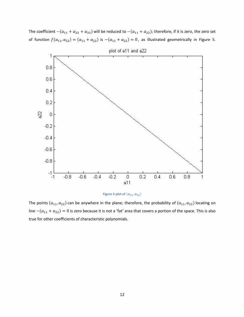
The coefficient −(𝑎11 + 𝑎22 + 𝑎33) will be reduced to −(𝑎11 + 𝑎22); therefore, if it is zero, the zero set
of function 𝑓(𝑎11, 𝑎22) = (𝑎11 + 𝑎22) is −(𝑎11 + 𝑎22) = 0 , as illustrated geometrically in Figure 5.
Figure 5 plot of (𝒂𝟏𝟏, 𝒂𝟐𝟐)
The points (𝑎11, 𝑎22) can be anywhere in the plane; therefore, the probability of (𝑎11, 𝑎22) locating on
line −(𝑎11 + 𝑎22) = 0 is zero because it is not a ‘fat’ area that covers a portion of the space. This is also
true for other coefficients of characteristic polynomials.
Page 17
13
4. Description of Research Results
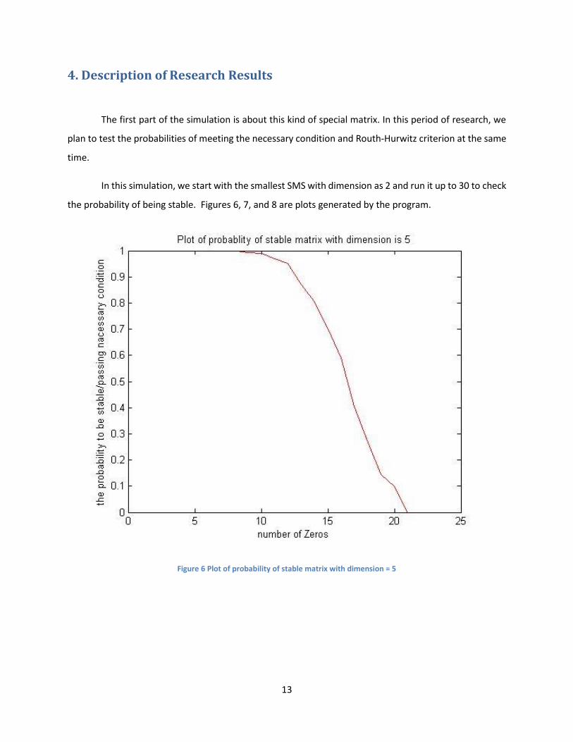
The first part of the simulation is about this kind of special matrix. In this period of research, we
plan to test the probabilities of meeting the necessary condition and Routh-Hurwitz criterion at the same
time.
In this simulation, we start with the smallest SMS with dimension as 2 and run it up to 30 to check
the probability of being stable. Figures 6, 7, and 8 are plots generated by the program.
Figure 6 Plot of probability of stable matrix with dimension = 5
Page 18
14
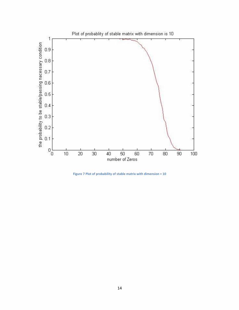
Figure 7 Plot of probability of stable matrix with dimension = 10
Page 19
15
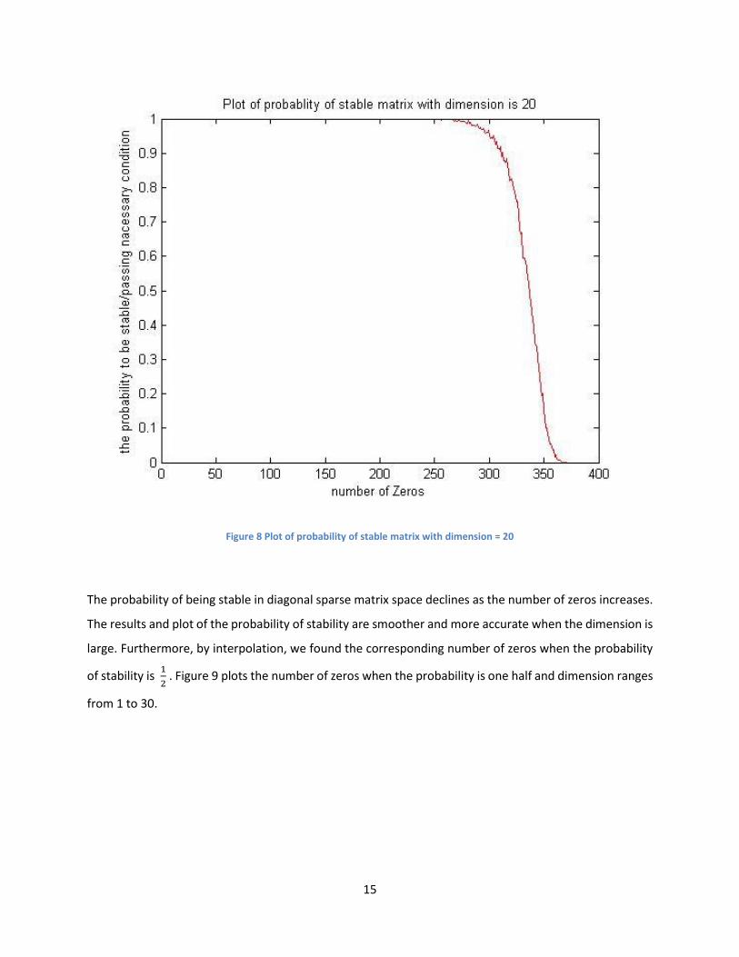
Figure 8 Plot of probability of stable matrix with dimension = 20
The probability of being stable in diagonal sparse matrix space declines as the number of zeros increases.
The results and plot of the probability of stability are smoother and more accurate when the dimension is
large. Furthermore, by interpolation, we found the corresponding number of zeros when the probability
of stability is 1
2 . Figure 9 plots the number of zeros when the probability is one half and dimension ranges
from 1 to 30.
Page 20
16
Figure 9 Plot of dimension and number of zeros when P = 0.5
After fitting the data into a function, we found the two quantities have a quadratic relation, with 95%
confidence bound, illustrated as follows (n is the number of zeros, and d is the dimension):
𝑛 = 𝑝1𝑑2 + 𝑝2𝑑 + 𝑝3
Here 𝑝1 = 0.958 (0.9531, 0.9628), 𝑝2 = −2.495(−2.65, −2.34), 𝑝3 = 4.21(3.618, 5.252).
Another interesting part of this simulation is for arbitrary sparse matrix systems. With a probability of p,
the conditional probability of being stable given it met the necessary condition can be calculated by a
great number of iterations. Since we need to compute the necessary condition only once for a random
sparse matrix system by sampling the positions of zero entries and nonzero ones, to see whether it is
stable or not, we need to sample many more matrices for stability check. We start by sampling 500
matrices and find that the simulation runs well when there are few zeros in the matrix, but when the
number of zeros grows, the conditional probability drops pretty fast. To improve the performance, we
Page 21
17
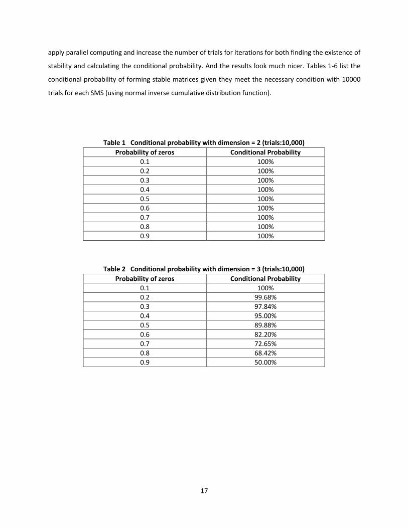
apply parallel computing and increase the number of trials for iterations for both finding the existence of
stability and calculating the conditional probability. And the results look much nicer. Tables 1-6 list the
conditional probability of forming stable matrices given they meet the necessary condition with 10000
trials for each SMS (using normal inverse cumulative distribution function).
Table 1 Conditional probability with dimension = 2 (trials:10,000)
Probability of zeros Conditional Probability
0.1 100%
0.2 100%
0.3 100%
0.4 100%
0.5 100%
0.6 100%
0.7 100%
0.8 100%
0.9 100%
Table 2 Conditional probability with dimension = 3 (trials:10,000)
Probability of zeros Conditional Probability
0.1 100%
0.2 99.68%
0.3 97.84%
0.4 95.00%
0.5 89.88%
0.6 82.20%
0.7 72.65%
0.8 68.42%
0.9 50.00%
Page 22
18
Table 3 Conditional probability with dimension = 4 (trials:10,000)
Probability of zeros Conditional Probability
0.1 100%
0.2 100%
0.3 99.46%
0.4 98.09%
0.5 92.98%
0.6 87.19%
0.7 71.43%
0.8 59.09%
0.9 33.33%
Table 4 Conditional probability with dimension = 5 (trials:10,000)
Probability of zeros Conditional Probability
0.1 100%
0.2 100%
0.3 100%
0.4 99.43%
0.5 97.55%
0.6 92.71%
0.7 76.34%
0.8 60.00%
0.9 20.00%
Table 5 Conditional probability with dimension = 6 (trials:10,000)
Probability of zeros Conditional Probability
0.1 100%
0.2 100%
0.3 100%
0.4 99.89%
0.5 98.85%
0.6 94.78%
0.7 83.33%
0.8 75.00%
0.9 50.00%
Page 23
19
.
Note that the conditional probability drops quickly when the probability of assigning zeros reaches 0.6.
We expected that the conditional probabilities are very close to each other; however, limited trials for
large matrices potentially skew the results. The discussion of results and some improvements will be
presented in the next chapter.
Table 6 Conditional probability with dimension = 7 (trials:10,000)
Probability of zeros Conditional Probability
0.1 99.94%
0.2 99.51%
0.3 98.11%
0.4 97.02%
0.5 94.81%
0.6 89.27%
0.7 78.00%
0.8 48.15%
0.9 40.00%
Page 24
20
5. Evaluation of Research Results and Methods and Improvements
The central part of this simulation aims to generate random numbers to fill the zero entries or
nonzero entries defined by sparse matrix systems, and the aim of this simulation is to test how effective
the necessary condition is for discerning the stability of a sparse matrix system.
We tried three different random functions to generate sparse matrix systems, as suggested
above. Drawing numbers from a standard normal distribution is the easiest method to generate random
numbers; however, after using this method, we found that the time lapse is pretty long, because the
possibility of generating a stable matrix is quite small if we do not let the number be more negative. And
if we deduct 0.1 from the random number for standard normal distribution, the running time is shorter.
The random number generated by normal inverse cumulative distribution function took the longest time,
three time as long as the normal distribution shifted left by 0.1.
The performances of different methods can be measured by both running time and conditional
probability. Furthermore, running time is influenced by two factors: first, the time complexity of functions
utilized by the algorithm, and second, the possibility to form a stable matrix. The first factor is easy to
understand: normal inverse cumulative distribution function is more complicated than normally
distributed random numbers function; therefore, the running time is less for using the latter if keeping
other factors the same. On the other hand, matrices generated by such methods cannot be guaranteed
to be stable. As mentioned in the algorithm description, the iterations in finding a stable matrix cover
most of the time taken into account. If the possibility to form a stable random matrix is too low, the
machine needs to go through nearly all the iterations, which is the worst case. Compared to the random
number generation methods, normal inverse cumulative distribution function would result in the highest
possibility to generate a stable matrix; thus to some extent, from the perspective of the number of
iterations, the normal inverse cumulative distribution function saves more time. Since by the normal
inverse cumulative distribution function gives a higher possibility to generate stable matrices if sparse
matrix systems pass the necessary condition, the conditional probability it gives is more accurate.
However, there is also a very important limitation of this simulation. The number of trials to
calculate the conditional probability is limited. When the possibility of assigning zeros in matrices becomes
larger, potentially the number of trials in this step is relatively small to generate a stable matrix. As a
result, we may miss a sparse matrix system, meeting the necessary condition, which has the potential to
Page 25
21
be stable. Therefore, to improve the accuracy, two possible methods can be implemented: 1) Improve the
random number generation mechanism and 2) increase the number of trials in the simulation.
In order to compare different methods, we conduct some further simulations and record the
conditional probability and running time. If we increase the number of trials from 10,000 to 100,000, the
results are better. Table 7 lists results for sparse matrix systems with dimension as 4.
Table 7 suggests when there are more trials, the simulation will diminish the differences given
different probabilities. We assume that given enough trials and optimized algorithms for random number
generation mechanisms, the conditional probabilities of different likelihoods of zeros are very close.
As for the running time, we compare the two methods using normal distribution random number
function (randn-0.1 and randn). The results are shown in Table 8.
We found that when we sample smaller dimension sparse matrix systems, the running times are
nearly identical; the reason is that, keeping the number of iterations fixed, for small sparse matrix
systems, stable matrices are easy to generate since there are not many zeros. Thus for both methods,
we do not need to run through all iterations; instead, only a few iterations are needed, and as a result,
two methods do not differentiate the result much. For medium sized matrices, the differences emerge:
randn-0.1 is faster than randn() since it is more likely to generate stable matrices. However, for even
Table 7 Conditional probability with dimension = 4 (trials :100,000)
Probability of zeros Conditional Probability
0.1 100%
0.2 99.92%
0.3 99.43%
0.4 97.77%
0.5 94.08%
0.6 87.03%
0.7 75.57%
0.8 58.26%
0.9 35.19%
Table 8 Running time comparison (trials:10000)
dimension randn-0.1 randn
2 450.228048 450.326511
3 478.347626 473.296798
4 512.650216 537.030156
5 556.782177 584.823447
6 620.813344 652.430190
7 747.353359 745.712389
Page 26
22
larger matrices, the running times are again close. We assume that this is actually not accurate enough
due to the limitation of the number of iterations. The difference between the two methods will be
obvious by increasing the number of iterations greatly.
The performance of randn-0.1 looks approximately the same for sparse matrix systems, if we keep
the number of trials fixed. But when many zeros exist, the results are very volatile. Considering the running
time metric, we think randn-0.1 works better. The results for a sparse matrix system of dimension 5 and
7 are shown in tables 9 and 10.
Table 9 Conditional probability generated by randn-0.1 and rand (trials: 10,000, dimension: 5)
Probability of zeros randn-0.1 randn
0.1 100% 100%
0.2 100% 100%
0.3 99.90% 99.90%
0.4 99.77% 99.21%
0.5 96.85% 97.10%
0.6 89.42% 92.61%
0.7 83.09% 81.69%
0.8 57.14% 41.38%
0.9 0 0
Table 10 Conditional probability generated by randn-0.1 and rand (trials: 10,000, dimension: 7)
Probability of zeros randn-0.1 randn
0.1 100% 99.90%
0.2 99.40% 99.30%
0.3 98.10% 98.90%
0.4 97.22% 97.74%
0.5 94.85% 94.54%
0.6 88.20% 90.33%
0.7 73.13% 82.11%
0.8 55.88% 50.00%
0.9 0 0
Page 27
23
6. Conclusion and Future Work
We have researched how effective the necessary condition is for testing the stability of sparse
matrix systems: the necessary condition is very effective if we have enough trials and the sparse matrices
meeting the necessary condition are very like to have at least one stable matrix. When the expectation of
the number of zeros in sparse matrix systems become larger, the simulation will be likely to present results
with large deviations if the random generated matrices are not stable with limited number of iterations.
Therefore, the next step in this research should be to find a random number generation method that can
more likely yield stable matrices and larger scale simulations.
Page 28
24
References
[1] Newman, M. E. J., D. J. Watts, and S. H. Strogatz. “Random Graph Models of Social Networks.”
Proceedings of the National Academy of Sciences 99. Supplement 1 (2002): 2566-2572.
[2] Barabási, A., R. Albert, and H. Jeong. “Mean-Field Theory for Scale-Free Random Networks.” Physica
A: Statistical Mechanics and its Applications 272.1-2 (1999): 173-187.
[3] Baillieul, J., and J. A. Panos. “Control and Communication Challenges in Networked Real-Time
Systems.” Proc. IEEE 95.1 (2007): 9-28.
[4] Jadbabaie, A., J. Lin, and A.S. Morse. “Correction to ‘Coordination of Groups of Mobile Autonomous
Agents Using Nearest Neighbor Rules.’” IEEE Transactions on Automatic Control 48.9 (2003): 1675-
1675.
[5] Sundaram, S., and C.N. Hadjicostis. “Distributed Function Calculation via Linear Iterative Strategies
in the Presence of Malicious Agents.” IEEE Transactions on Automatic Control 56.7 (2011): 1495-
1508.
[6] Nedic, A., and A. Ozdaglar. “Distributed Subgradient Methods for Multi-Agent Optimization.” IEEE
Transactions on Automatic Control 54.1 (2009): 48-61.
[7] Desai, J.P., J.P. Ostrowski, and V. Kumar. “Modeling and Control of Formations of Nonholonomic
Mobile Robots.” IEEE Trans. Robot. Automat. 17.6 (2001): 905-908.
[8] Mesbahi, M., and M. Egerstedt. Graph Theoretic Methods in Multiagent Networks. Princeton:
Princeton University Press, 2010.
[9] Shamma, S. Cooperative Control of Distributed Multi-Agent Systems. Chichester, England: John
Wiley & Sons, 2008.
[10] Horn, R. A., and R. J. Charles. Matrix Analysis. Cambridge, UK: Cambridge University Press, 1985.
[11] Belabbas, M.-A. “Sparse Stable Systems.” Systems & Control Letters 62.10 (2013): 981-987.