The Garden-Hose Model

Harry Buhrman1,2, Serge Fehr1, Christian Schaffner2,1, and Florian Speelman1,2

1 Centrum Wiskunde & Informatica (CWI), The Netherlands2 University of Amsterdam, The Netherlands

Email: h.buhrman@cwi.nl, s.fehr@cwi.nl, c.schaffner@uva.nl, f.speelman@cwi.nl

Abstract. We define a new model of communication complexity, called the garden-hose model.Informally, the garden-hose complexity of a function f : 0, 1n × 0, 1n → 0, 1 is given by theminimal number of water pipes that need to be shared between two parties, Alice and Bob, in orderfor them to compute the function f as follows: Alice connects her ends of the pipes in a way thatis determined solely by her input x ∈ 0, 1n and, similarly, Bob connects his ends of the pipes ina way that is determined solely by his input y ∈ 0, 1n. Alice turns on the water tap that she alsoconnected to one of the pipes. Then, the water comes out on Alice’s or Bob’s side depending onthe function value f(x, y).We prove almost-linear lower bounds on the garden-hose complexity for concrete functions like innerproduct, majority, and equality, and we show the existence of functions with exponential garden-hose complexity. Furthermore, we show a connection to classical complexity theory by proving thatall functions computable in log-space have polynomial garden-hose complexity.We consider a randomized variant of the garden-hose complexity, where Alice and Bob hold pre-shared randomness, and a quantum variant, where Alice and Bob hold pre-shared quantum entan-glement, and we show that the randomized garden-hose complexity is within a polynomial factorof the deterministic garden-hose complexity. Examples of (partial) functions are given where thequantum garden-hose complexity is logarithmic in n while the classical garden-hose complexity canbe lower bounded by nc for constant c > 0.Finally, we show an interesting connection between the garden-hose model and the (in)security ofa certain class of quantum position-verification schemes.

1 Introduction

The garden-hose model. On a beautiful sunny day, Alice and Bob relax in their neigh-boring gardens. It happens that their two gardens share s water pipes, labeled by the numbers1, 2, . . . , s. Each of these water pipes has one loose end in Alice’s and the other loose end inBob’s garden. For the fun of it, Alice and Bob play the following game. Alice uses pieces of hoseto locally connect some of the pipe ends that are in her garden with each other. For example,she might connect pipe 2 with pipe 5, pipe 4 with pipe 9, etc. Similarly, Bob locally connectssome of the pipe ends that are in his garden; for instance pipe 1 with pipe 4, etc. We note thatno T-pieces (nor more complicated constructions), which connect two or more pipes to one (orvice versa) are allowed. Finally, Alice connects a water tap to one of her ends of the pipes,e.g., to pipe 3 and she turns on the tap. Alice and Bob observe which of the two gardens getssprinkled. It is easy to see that since Alice and Bob only use simple one-to-one connections,there is no “deadlock” possible and the water will indeed eventually come out on one of the twosides. Which side it is obviously depends on the respective local connections.

Now, say that Alice connects her ends of the pipes (and the tap) not in a fixed way, buther choice of connections depends on a private bit string x ∈ 0, 1n; for different strings xand x′, she may connect her ends of the pipes differently. Similarly, Bob’s choice which pipesto connect depends on a private bit string y ∈ 0, 1n. These strategies then specify a functionf : 0, 1n × 0, 1n → 0, 1 as follows: f(x, y) is defined to be 0 if, using the connectionsdetermined by x and y respectively, the water ends up on Alice’s side, and f(x, y) is 1 if thewater ends up on Bob’s side.

Switching the point of view, we can now take an arbitrary Boolean function f : 0, 1n ×0, 1n → 0, 1 and ask: How can f be computed in the garden-hose model? How do Aliceand Bob have to choose their local connections, and how many water pipes are necessary for

computing f in the garden-hose model? We stress that Alice’s choice for which pipes to connectmay only depend on x but not on y, and vice versa; this is what makes the above questionsnon-trivial.

In this paper, we introduce and put forward the notion of garden-hose complexity. Fora Boolean function f : 0, 1n × 0, 1n → 0, 1, the garden-hose complexity GH (f) of fis defined to be the minimal number s of water pipes needed to compute f in the garden-hose model. It is not too hard to see that GH (f) is well defined (and finite) for any functionf : 0, 1n × 0, 1n → 0, 1.

This new complexity notion opens up a large spectrum of natural problems and questions.What is the (asymptotic or exact) garden-hose complexity of natural functions, like equality,inner product etc.? How hard is it to compute the garden-hose complexity in general? Howis the garden-hose complexity related to other complexity measures? What is the impact ofrandomness, or entanglement? Some of these questions we answer in this work; others remainopen.

Lower and upper bounds. We show a near-linear Ω(n/ log(n)) lower bound on the garden-hose complexity GH (f) for a natural class of functions f : 0, 1n×0, 1n → 0, 1. This classof functions includes the mod-2 inner-product function, the equality function, and the majorityfunction. For the former two, this bound is rather tight, in that for these two functions wealso show a linear upper bound. For the majority function, the best upper bound we know isquadratic. Recently, Margalit and Matsliah improved our upper bound for the equality functionwith the help of the IBM SAT-Solver [MM12] to approximately 1.448n, and the question ofhow many water pipes are necessary to compute the equality function in the garden-hose modelfeatured as April 2012’s “Ponder This” puzzle on the IBM website3. The exact garden-hosecomplexity of the equality function is still unknown, though; let alone of other functions.

By using a counting argument, we show the existence of functions with exponential garden-hose complexity, but so far, no such function is known explicitly.

Connections to other complexity notions. We show that every function f : 0, 1n ×0, 1n → 0, 1 that is log-space computable has polynomial garden-hose complexity. And, viceversa, we show that every function with polynomial garden-hose complexity is, up to local pre-processing, log-space computable. As a consequence, we obtain that the set of functions withpolynomial garden-hose complexity is exactly given by the functions that can be computed byarbitrary local pre-processing followed by a log-space computation.

We also point out a connection to communication complexity by observing that, for anyfunction f : 0, 1n × 0, 1n → 0, 1, the one-way communication complexity of f is a lowerbound on GH (f) log(GH (f)).

Randomized and quantum garden-hose complexity. We consider the following natu-ral variants of the garden-hose model. In the randomized garden-hose model, Alice and Bobadditionally share a uniformly random string r, and the water is allowed to come out on thewrong side with small probability ε. Similarly, in the quantum garden-hose model, Alice andBob additionally hold an arbitrary entangled quantum state and their wiring strategies can de-pend on the outcomes of measuring this state before playing the garden-hose game. Again, thewater is allowed to come out on the wrong side with small probability ε. Based on the observedconnections of the garden-hose complexity to log-space computation and to one-way communi-cation complexity, we can show that the resulting notion of randomized garden-hose complexityGHε(f) is polynomially related to GH (f). For the resulting notion of quantum garden-hosecomplexity GH Q

ε (f), we can show a separation (for a partial function) from GHε(f).

3 http://ibm.co/I7yvMz

2

Application to quantum position-verification. Finally, we show an interesting connectionbetween the garden-hose model and the (in)security of a certain class of quantum position-verification schemes. The goal of position-verification is to verify the geographical position posof a prover P by means of sending messages to P and measuring the time it takes P to reply.Position-verification with security against collusion attacks, where different attacking partiescollaborate in order to try to fool the verifiers, was shown to be impossible in the classicalsetting by [CGMO09], and in the quantum setting by [BCF+11], if there is no restriction putupon the attackers. In the quantum setting, this raises the question whether there exist schemesthat are secure in case the attackers’ quantum capabilities are limited.

We consider a simple and natural class of quantum position-verification schemes; each schemePVfqubit in the class is specified by a Boolean function f : 0, 1n × 0, 1n → 0, 1. Theseschemes may have the desirable property that the more classical resources the honest users useto faithfully execute the scheme, the more quantum resources the adversary needs in order tobreak it. It turns out that there is a one-to-one correspondence between the garden-hose gameand a certain class of attacks on these schemes, where the attackers teleport a qubit back andforth using a supply of EPR pairs. As an immediate consequence, the (quantum) garden-hosecomplexity of f gives an upper bound on the number of EPR pairs the attackers need in order tobreak the scheme PVfqubit. As a corollary, we obtain the following interesting connection betweenproving the security of quantum protocols and classical complexity theory: If there is an f in Psuch that there is no way of attacking scheme PVfqubit using a polynomial number of EPR pairs,then P 6= L. Vice versa, our approach may lead to practical secure quantum position-verificationschemes whose security is based on classical complexity-theoretical assumptions such as P isdifferent from L. However, so far it is still unclear whether the garden-hose complexity by anymeans gives a lower bound on the number of EPR pairs needed; this remains to be furtherinvestigated.

2 The Garden-Hose Model

2.1 Definition

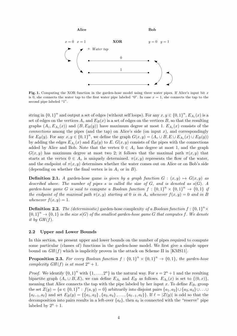
Alice and Bob get n-bit input strings x and y, respectively. Their goal is to “compute” an agreed-upon Boolean function f : 0, 1n×0, 1n → 0, 1 on these inputs, in the following way. Aliceand Bob have s water pipes between them, and, depending on their respective classical inputsx and y, they connect (some of) their ends of the pipes with pieces of hose. Additionally, Aliceconnects a water tap to one of the pipes. They succeed in computing f in the garden-hosemodel, if the water comes out on Alice’s side whenever f(x, y) = 0, and the water comes out onBob’s side whenever f(x, y) = 1. Note that it does not matter out of which pipe the water flows,only on which side it flows. What makes the game non-trivial is that Alice and Bob must dotheir “plumbing” based on their local input only, and they are not allowed to communicate. Werefer to Figure 1 for an illustration of computing the XOR function in the garden-hose model.

We formalize the above description of the garden-hose game, given in terms of pipes andhoses etc., by means of rigorous graph-theoretic terminology. However, we feel that the aboveterminology captures the notion of a garden-hose game very well, and thus we sometimes usethe above “watery” terminology. We start with a balanced bi-partite graph (A ∪ B,E) whichis 1-regular and where the cardinality of A and B is |A| = |B| = s, for an arbitrary larges ∈ N. We slightly abuse notation and denote both the vertices in A and in B by the integers1, . . . , s. If we need to distinguish i ∈ A from i ∈ B, we use the notation iA and iB. We mayassume that E consists of the edges that connect i ∈ A with i ∈ B for every i ∈ 1, . . . , s, i.e.,E =

iA, iB

: 1 ≤ i ≤ s

. These edges in E are the pipes in the above terminology. We now

extend the graph to (A∪B,E) by adding a vertex 0 to A, resulting in A = A∪0. This vertexcorresponds to the water tap, which Alice can connect to one of the pipes. Given a Booleanfunction f : 0, 1n×0, 1n → 0, 1, consider two functions EA and EB; both take as input a

3

0

1

x = 0 x = 1

Alice

y = 0 y = 1

Bob

XOR

Water tap

Fig. 1. Computing the XOR function in the garden-hose model using three water pipes. If Alice’s input bit xis 0, she connects the water tap to the first water pipe labeled “0”. In case x = 1, she connects the tap to thesecond pipe labeled “1”.

string in 0, 1n and output a set of edges (without self loops). For any x, y ∈ 0, 1n, EA(x) is aset of edges on the vertices A and EB(x) is a set of edges on the vertices B, so that the resultinggraphs (A, EA(x)) and (B,EB(y)) have maximum degree at most 1. EA(x) consists of theconnections among the pipes (and the tap) on Alice’s side (on input x), and correspondinglyfor EB(y). For any x, y ∈ 0, 1n, we define the graph G(x, y) = (A ∪B,E ∪EA(x) ∪EB(y))by adding the edges EA(x) and EB(y) to E. G(x, y) consists of the pipes with the connectionsadded by Alice and Bob. Note that the vertex 0 ∈ A has degree at most 1, and the graphG(x, y) has maximum degree at most two 2; it follows that the maximal path π(x, y) thatstarts at the vertex 0 ∈ A is uniquely determined. π(x, y) represents the flow of the water,and the endpoint of π(x, y) determines whether the water comes out on Alice or on Bob’s side(depending on whether the final vertex is in A or in B).

Definition 2.1. A garden-hose game is given by a graph function G : (x, y) 7→ G(x, y) asdescribed above. The number of pipes s is called the size of G, and is denoted as s(G). Agarden-hose game G is said to compute a Boolean function f : 0, 1n × 0, 1n → 0, 1 ifthe endpoint of the maximal path π(x, y) starting at 0 is in A whenever f(x, y) = 0 and in Bwhenever f(x, y) = 1.

Definition 2.2. The (deterministic) garden-hose complexity of a Boolean function f : 0, 1n×0, 1n → 0, 1 is the size s(G) of the smallest garden-hose game G that computes f . We denoteit by GH (f).

2.2 Upper and Lower Bounds

In this section, we present upper and lower bounds on the number of pipes required to computesome particular (classes of) functions in the garden-hose model. We first give a simple upperbound on GH (f) which is implicitly proven in the attack on Scheme II in [KMS11].

Proposition 2.3. For every Boolean function f : 0, 1n × 0, 1n → 0, 1, the garden-hosecomplexity GH (f) is at most 2n + 1.

Proof. We identify 0, 1n with 1, . . . , 2n in the natural way. For s = 2n + 1 and the resultingbipartite graph (A ∪ B,E), we can define EA and EB as follows. EA(x) is set to (0, x),meaning that Alice connects the tap with the pipe labeled by her input x. To define EB, groupthe set Z(y) = a ∈ 0, 1n : f(a, y) = 0 arbitrarily into disjoint pairs a1, a2∪a3, a4∪ . . .∪a`−1, a` and set EB(y) = a1, a2 , a3, a4 , . . . , a`−1, a`. If ` = |Z(y)| is odd so that thedecomposition into pairs results in a left-over a`, then a` is connected with the “reserve” pipelabeled by 2n + 1.

4

By construction, if x ∈ Z(y) then x = ai for some i, and thus pipe x = ai is connected onBob’s side with pipe ai−1 or ai+1, depending on the parity of i, or with the “reserve” pipe, andthus π(x, y) is of the form π(x, y) = (0, xA, xB, vB, vA), ending in A. On the other hand, ifx 6∈ Z(y), then pipe x is not connected on Bob’s side, and thus π(x, y) = (0, xA, xB), ending inB. This proves the claim. ut

We notice that we can extend this proof to show that the garden-hose complexity GH (f) isat most 2D(f)+1 − 1, where D(f) is the deterministic communication complexity of f . SeeAppendix A for a sketch of the method.

Definition 2.4. We call a function f injective for Alice, if for every two different inputs x andx′ there exists y such that f(x, y) 6= f(x′, y). We define injective for Bob in an analogous way:for every y 6= y′, there exists x such that f(x, y) 6= f(x, y′) holds.

Proposition 2.5. If f is injective for Bob or f is injective for Alice, then4

GH (f) log(GH (f)) ≥ n .

Proof. We give the proof when f is injective for Bob. The proof for the case where f is injectivefor Alice is the same. Consider a garden-hose game G that computes f . Let s be its size s(G).Since, on Bob’s side, every pipe is connected to at most one other pipe, there are at mostss = 2s log(s) possible choices for EB(y), i.e., the set of connections on Bob’s side. Thus, if2s log(s) < 2n, it follows from the pigeonhole principle that there must exist y and y′ in 0, 1nfor which EB(y) = EB(y′), and thus for which G(x, y) = G(x, y′) for all x ∈ 0, 1n. But thiscannot be since G computes f and f(x, y) 6= f(x, y′) for some x due to the injectivity for Bob.Thus, 2s log(s) ≥ 2n which implies the claim. ut

We can use this result to obtain an almost linear lower bound for several functions that areoften studied in communication complexity settings such as:

– Bitwise inner product: IP(x, y) =∑

i xiyi (mod 2)– Equality: EQ(x, y) = 1 if and only if x = y– Majority: MAJ(x, y) = 1 if and only if

∑i xiyi ≥ d

n2 e

The first two of these functions are injective for both Alice and Bob, while majority is injectivefor inputs of Hamming weight at least n/2, giving us the following corollary.

Corollary 2.6. The functions bitwise inner product, equality and majority have garden-hosecomplexity in Ω( n

log(n)).

By considering the water pipes that actually get wet, one can show a lower bound of n pipes forequality [Pie11]. On the other hand, we can show upper bounds that are linear for the bitwiseinner product and equality, and quadratic in case of majority. We refer to [Spe11] for the proofof the following proposition.

Proposition 2.7. In the garden-hose model, the equality function can be computed with 3n+ 1pipes, the bitwise inner product with 4n+ 1 pipes and majority with (n+ 2)2 pipes.

In general, garden-hose protocols can be transformed into (one-way) communication proto-cols by Alice sending her connections EA(x) to Bob which requires at most GH (f) log(GH (f))bits of communication. Bob can then locally compute the function by combining Alice’s mes-sage with EB(y) and checking where the water exits.5 We summarize this observation in thefollowing proposition.

4 All logarithms in this paper are with respect to base 2.5 In fact, garden-hose protocols can even be transformed into communication protocols in the more restrictive

simultaneous-message-passage model, where Alice and Bob send simultaneous messages consisting of theirconnections EA(x) and EB(y) to the referee who then computes the function. The according statements ofPropositions 2.8, 2.19 and 2.20 can be derived analogously.

5

Proposition 2.8. Let D1(f) denote the deterministic one-way communication complexity off . Then, D1(f) ≤ GH (f) log(GH (f)).

As a consequence, lower bounds on the communication complexity carry over to the garden-hose complexity (up to logarithmic factors). Notice that this technique will never give lowerbounds that are better than linear, as the communication-complexity problem can always besolved by sending the entire input to the other party. It is an interesting open problem to showsuper-linear lower bounds in the garden-hose model, e.g. for the majority function.

Proposition 2.9. There exist functions f : 0, 1n × 0, 1n → 0, 1 for which GH (f) isexponential.

Proof. The existence of functions with an exponential garden-hose complexity can be shown bya simple counting argument. There are 222n different functions f(x, y). For a given size s = s(G)of G, for every x ∈ 0, 1n, there are at most (s+ 1)s+1 ways to choose the connections EA(x)on Alice’s side, and thus there are at most ((s+ 1)s+1)2n = 22n(s+1) log(s+1) ways to choose thefunction EA . Similarly for EB, there are at most 22ns log(s) ways to choose EB. Thus, there areat most 22·2n(s+1) log(s+1) ways to choose G of size s. Clearly, in order for every function f tohave a G of size s that computes it, we need that 2 · 2n(s + 1) log(s + 1) ≥ 22n, and thus that(s+ 1) log(s+ 1) ≥ 2n−1, which means that s must be exponential. ut

2.3 Polynomial Garden-Hose Complexity and Log-Space Computations

A family of Boolean functions fnn∈N is log-space computable if there exists a deterministicTuring machine M and a constant c, such that for any n-bit input x, M outputs the correctoutput bit fn(x), and at most c · log n locations of M ’s work tapes are ever visited by M ’s headduring computation.

Definition 2.10. We define L(2), called logarithmic space with local pre-processing, to be theclass of Boolean functions f(x, y) for which there exists a Turing machine M and two arbi-trary functions α(x), β(y), such that6 M(α(x), β(y)) = f(x, y) and M(α(x), β(y)) runs in spacelogarithmic in the size of the original inputs |x|+ |y|.

This definition can be extended in a natural way by considering Turing machines and circuitscorresponding to various complexity classes, and by varying the number of players. For example,a construction as in Proposition 2.3 and a similar reasoning as in Proposition 2.14 below canbe used to show that every Boolean function is contained in PSPACE(2). As main result of thissection, we show that our newly defined class L(2) is equivalent to functions with polynomialgarden-hose complexity. We leave it for future research to study intermediate classes such asAC0

(2) which are related to the polynomial hierarchy of communication complexity [BFS86].

Theorem 2.11. The set of functions f with polynomial garden-hose complexity GH (f) is equalto L(2).

The two directions of the theorem follow from Theorem 2.12 and Proposition 2.14.

Theorem 2.12. If f : 0, 1n × 0, 1n → 0, 1 is log-space computable, then GH (f) is poly-nomial in n.

Proof (sketch, the full proof can be found as Appendix B.1). Let M be the deterministic log-space Turing machine deciding f(x, y) = 0. Using techniques from [LMT97], M can be madereversible incurring only a constant loss in space. As M is a log-space machine, it has at most

6 For simplicity of notation, we give two arguments to the Turing machine whose concatenation is interpretedas the input.

6

polynomially many configurations. The idea for the garden-hose strategy is to label the pipeswith those configurations of the machine M where the input head of M “switches sides” fromthe x-part of the input to the y-part or vice versa. Thanks to the reversibility of M , the playerscan then use one-to-one connections to wire up (depending on their individual inputs) the openends of the pipes on their side, so that eventually the water flow corresponds to M ’s computationof f(x, y). ut

In the garden-hose model, we allow Alice and Bob to locally pre-process their inputs beforecomputing their wiring. Therefore, it immediately follows from Theorem 2.12 that any functionf in L(2) has polynomial garden-hose complexity, proving one direction of Theorem 2.11.

We saw in Proposition 2.9 that there exist functions with large garden-hose complexity.However, a negative implication of Theorem 2.12 is that proving the existence of a polynomial-time computable function f with exponential garden-hose complexity is at least as hard asseparating L from P, a long-standing open problem in complexity theory.

Corollary 2.13. If there exists a function f : 0, 1n × 0, 1n → 0, 1 in P that has super-polynomial garden-hose complexity, then P 6= L.

It remains to prove the other inclusion of Theorem 2.11.

Proposition 2.14. Let f : 0, 1n × 0, 1n → 0, 1 be a Boolean function. If GH (f) ispolynomial (in n), then f is in L(2).

Proof. Let G be the garden-hose game that achieves s(G) = GH (f). We write s for s(G), thenumber of pipes, and we let EA and EB be the underlying edge-picking functions, which oninput x and y, respectively, output the connections that Alice and Bob apply to the pipes. Notethat by assumption, s is polynomial. Furthermore, by the restrictions on EA and EB, on anyinput, they consist of at most (s+ 1)/2 connections.

We need to show that f is of the form f(x, y) = g(α(x), β(y)), where α and β are arbitraryfunctions 0, 1n → 0, 1m, g : 0, 1m × 0, 1m → 0, 1 is log-space computable, and m ispolynomial in n. We define α and β as follows. For any x, y ∈ 0, 1n, α(x) is simply a naturalencoding of EA(x) into 0, 1m, and β(y) is a natural encoding of EB(y) into 0, 1m. In thehose-terminology we say that α(x) is a binary encoding of the connections of Alice, and β(y) isa binary encoding of the connections of Bob. Obviously, these encodings can be done with mof polynomial size. Given these encodings, finding the endpoint of the maximum path π(x, y)starting in 0 can be done with logarithmic space: at any point during the computation, theTuring machine only needs to maintain a pointer to the position of the water and a binary flagto remember on which side of the input tape the head is. Thus, the function g that computesg(α(x), β(y)) = f(x, y) is log-space computable in m and thus also in n. ut

2.4 Randomized Garden-Hose Complexity

It is natural to study the setting where Alice and Bob share a common random string andare allowed to err with some probability ε. More formally, we let the players’ local strategiesEA(x, r) and EB(y, r) depend on the shared randomness r and write Gr(x, y) = f(x, y) if theresulting garden-hose game Gr(x, y) computes f(x, y).

Definition 2.15. Let r be the shared random string. The randomized garden-hose complexityof a Boolean function f : 0, 1n×0, 1n → 0, 1 is the size s(Gr) of the smallest garden-hosegame Gr such that ∀x, y : Prr[Gr(x, y) = f(x, y)] ≥ 1 − ε. We denote this minimal size byGHε(f).

In Appendix B.2, we show that the error probability can be made exponentially small byrepeating the protocol a polynomial number of times.

7

Proposition 2.16. Let f : 0, 1n × 0, 1n → 0, 1 be a function such that GHε(f) is poly-nomial in n, with error ε ≤ 1

2 − n−c for a constant c > 0. For every constant d > 0 there exists

a polynomial q(·) such that GH 2−d(f) ≤ q(GHε(f)

).

Using this result, any randomized strategy can be turned into a deterministic strategy withonly a polynomial overhead in the number of pipes.

Proposition 2.17. Let f : 0, 1n × 0, 1n → 0, 1 be a function such that GHε(f) is poly-nomial in n and ε ≤ 1

2 − nc for a constant c > 0. Then there exists a polynomial q(·) such that

GH (f) ≤ q(GHε(f)

).

Proof (sketch). By Proposition 2.16 there exists a randomized garden-hose protocol Gr(x, y) ofsize q(GHε(f)) with error probability at most 2−2n−1. The probability for a random string r tobe wrong for all inputs is at most 22n · 2−2n−1 < 1. In particular, there exists a string r whichworks for every input (x, y).

ut

Using this Proposition 2.17, we conclude that the lower bound from Proposition 2.9 carriesover to the randomized setting.

Corollary 2.18. There exist functions f : 0, 1n × 0, 1n → 0, 1 for which GHε(f) isexponential.

With the same reasoning as in Proposition 2.8, we get that lower bounds on the randomizedone-way communication complexity with public shared randomness carry over to the randomizedgarden-hose complexity (up to a logarithmic factor).

Proposition 2.19. Let R1,pubε (f) denote the minimum communication cost of a one-way-communication

protocol which computes f with an error ε using public shared randomness. Then, R1,pubε (f) ≤

GHε(f) log(GHε(f)).

For instance, the linear lower bound Rpubε (IP ) ∈ Ω(n) from [CG88] for the inner-productfunction yields GHε(IP ) ∈ Ω( n

logn).

2.5 Quantum Garden-Hose Complexity

Let us consider the setting where Alice and Bob share an arbitrary entangled quantum statebesides their water pipes. Depending on their respective inputs x and y, they can perform localquantum measurements on their parts of the entangled state and wire up the pipes depending onthe outcomes of these measurements. We denote the resulting quantum garden-hose complexitywith GH Q(f) in the deterministic case and with GH Q

ε (f) if errors are allowed.With the same reasoning as in Proposition 2.8, we get that lower bounds on the entanglement-

assisted one-way communication complexity carry over to the quantum garden-hose complexity(up to a logarithmic factor).

Proposition 2.20. For ε ≥ 0, let Q1ε(f) denote the minimum cost of an entanglement-assisted

one-way communication protocol which computes f with an error ε. Then, Q1ε(f) ≤ GH Q

ε (f) log(GH Qε (f)).

For instance, the lower bound Q1ε(IP ) ∈ Ω(n) which follows from results in [CDNT98] gives

GH Qε (IP ) ∈ Ω(n/ log n). For the disjointness function, Q1

ε(DISJ) ∈ Ω(√n) from [Raz03]

implies GH Qε (DISJ) ∈ Ω(

√n/ log n).

In Appendix D, we present partial functions which give a separation between the quantumand classical garden-hose complexity in the deterministic and in the randomized setting.

Theorem 2.21. There exist partial Boolean functions f and g such that

1. GH Q(f) ∈ O(log n) and GH (f) ∈ Ω( nlogn),

2. GH Qε (g) ∈ O(log n) and GHε(g) ∈ Ω(

√n

logn).

8

3 Application to Position-Based Quantum Cryptography

The goal of position-based cryptography is to use the geographical position of a party as itsonly “credential”. For example, one would like to send a message to a party at a geographicalposition pos with the guarantee that the party can decrypt the message only if he or she isphysically present at pos. The general concept of position-based cryptography was introducedby Chandran, Goyal, Moriarty and Ostrovsky [CGMO09].

A central task in position-based cryptography is the problem of position-verification. Wehave a prover P at position pos, wishing to convince a set of verifiers V0, . . . , Vk (at differentpoints in geographical space) that P is indeed at that position pos. The prover can run aninteractive protocol with the verifiers in order to convince them. The main technique for sucha protocol is known as distance bounding [BC94]. In this technique, a verifier sends a randomnonce to P and measures the time taken for P to reply back with this value. Assuming that thespeed of communication is bounded by the speed of light, this technique gives an upper boundon the distance of P from the verifier.

The problem of secure position-verification has been studied before in the field of wire-less security, and there have been several proposals for this task ([BC94,SSW03,VN04,Bus04][CH05,SP05,ZLFW06,CCS06]). However, [CGMO09] shows that there exists no protocol for se-cure position-verification that offers security in the presence of multiple colluding adversaries. Inother words, the set of verifiers cannot distinguish between the case when they are interactingwith an honest prover at pos and the case when they are interacting with multiple colludingdishonest provers, none of which is at position pos.

The impossibility result of [CGMO09] relies heavily on the fact that an adversary can locallystore all information he receives and at the same time share this information with other collud-ing adversaries, located elsewhere. Due to the quantum no-cloning theorem, such a strategy willnot work in the quantum setting, which opens the door to secure protocols that use quantum in-formation. The quantum model was first studied by Kent et al. under the name of “quantum tag-ging” [KMSB06,KMS11]. Several schemes were developed [KMS11,Mal10a,CFG+10,Mal10b,LL11]and proven later to be insecure. Finally in [BCF+11] it was shown that in general no uncon-ditionally secure quantum position-verification scheme is possible. Any scheme can be brokenusing a double exponential amount of EPR pairs in the size of the messages of the proto-col. Later, Beigi and Konig improved in [BK11] the double exponential dependence to singleexponential making use of port-based teleportation [IH08,IH09].

Due to the exponential overhead in EPR pairs, the general no-go theorem does not ruleout the existence of quantum schemes that are secure for all practical purposes. Such schemesshould have the property that the protocol, when followed honestly, is feasible, but cheating theprotocol requires unrealistic amounts of resources, for example EPR pairs or time.

3.1 A Single-Qubit Scheme

Our original motivation for the garden-hose model was to study a particular quantum proto-col for secure position verification, described in Figure 2. The protocol is of the generic formdescribed in Section 3.2 of [BCF+11]. In Step 0, the verifiers prepare challenges for the prover.In Step 1, they send the challenges, timed in such a way that they all arrive at the same timeat the prover. In Step 2, the prover computes his answers and sends them back to the verifiers.Finally, in Step 3, the verifiers verify the timing and correctness of the answer.

As in [BCF+11], we consider here for simplicity the case where all players live in one di-mension, the basic ideas generalize to higher dimensions. In one dimension, we can focus on thecase of two verifiers V0, V1 and an honest prover P in between them.

We minimize the amount of quantum communication in that only one verifier, say V0, sendsa qubit to the prover, whereas both verifiers send classical n-bit strings x, y ∈ 0, 1n that arriveat the same time at the prover. We fix a publicly known Boolean function f : 0, 1n×0, 1n →

9

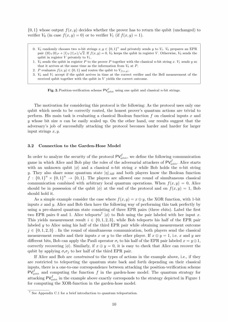
0, 1 whose output f(x, y) decides whether the prover has to return the qubit (unchanged) toverifier V0 (in case f(x, y) = 0) or to verifier V1 (if f(x, y) = 1).

0. V0 randomly chooses two n-bit strings x, y ∈ 0, 1n and privately sends y to V1. V0 prepares an EPRpair (|0〉V |0〉P + |1〉V |1〉P )/

√2. If f(x, y) = 0, V0 keeps the qubit in register V . Otherwise, V0 sends the

qubit in register V privately to V1.

1. V0 sends the qubit in register P to the prover P together with the classical n-bit string x. V1 sends y sothat it arrives at the same time as the information from V0 at P .

2. P evaluates f(x, y) ∈ 0, 1 and routes the qubit to Vf(x,y).

3. V0 and V1 accept if the qubit arrives in time at the correct verifier and the Bell measurement of thereceived qubit together with the qubit in V yields the correct outcome.

Fig. 2.Position-verification scheme PVfqubit using one qubit and classical n-bit strings.

The motivation for considering this protocol is the following: As the protocol uses only onequbit which needs to be correctly routed, the honest prover’s quantum actions are trivial toperform. His main task is evaluating a classical Boolean function f on classical inputs x andy whose bit size n can be easily scaled up. On the other hand, our results suggest that theadversary’s job of successfully attacking the protocol becomes harder and harder for largerinput strings x, y.

3.2 Connection to the Garden-Hose Model

In order to analyze the security of the protocol PVfqubit, we define the following communication

game in which Alice and Bob play the roles of the adversarial attackers of PVfqubit. Alice startswith an unknown qubit |φ〉 and a classical n-bit string x while Bob holds the n-bit stringy. They also share some quantum state |η〉AB and both players know the Boolean functionf : 0, 1n × 0, 1n → 0, 1. The players are allowed one round of simultaneous classicalcommunication combined with arbitrary local quantum operations. When f(x, y) = 0, Aliceshould be in possession of the qubit |φ〉 at the end of the protocol and on f(x, y) = 1, Bobshould hold it.

As a simple example consider the case where f(x, y) = x⊕ y, the XOR function, with 1-bitinputs x and y. Alice and Bob then have the following way of performing this task perfectly byusing a pre-shared quantum state consisting of three EPR pairs (three ebits). Label the firsttwo EPR pairs 0 and 1. Alice teleports7 |φ〉 to Bob using the pair labeled with her input x.This yields measurement result i ∈ 0, 1, 2, 3, while Bob teleports his half of the EPR pairlabeled y to Alice using his half of the third EPR pair while obtaining measurement outcomej ∈ 0, 1, 2, 3 . In the round of simultaneous communication, both players send the classicalmeasurement results and their inputs x or y to the other player. If x ⊕ y = 1, i.e. x and y aredifferent bits, Bob can apply the Pauli operator σi to his half of the EPR pair labeled x = y⊕1,correctly recovering |φ〉. Similarly, if x ⊕ y = 0, it is easy to check that Alice can recover thequbit by applying σiσj to her half of the third EPR pair.

If Alice and Bob are constrained to the types of actions in the example above, i.e., if theyare restricted to teleporting the quantum state back and forth depending on their classicalinputs, there is a one-to-one correspondence between attacking the position-verification schemePVfqubit and computing the function f in the garden-hose model. The quantum strategy for

attacking PVfqubit in the example above exactly corresponds to the strategy depicted in Figure 1for computing the XOR-function in the garden-hose model.

7 See Appendix C.1 for a brief introduction to quantum teleportation.

10

More generally, we can translate any strategy of Alice and Bob in the garden-hose modelto a perfect quantum attack of PVfqubit by using one EPR pair per pipe and performing Bellmeasurements where the players connect the pipes.

Our hope is that also the converse is true: if many pipes are required to compute f (saywe need super-polynomially many), then the number of EPR pairs needed for Alice and Bob

to successfully break PVfqubit with probability close to 1 by means of an arbitrary attack (notrestricted to Bell measurements on EPR pairs) should also be super-polynomial.

The examples of (partial) functions from Theorem 2.21 show that the classical garden-hose

complexity GH (f) does not capture the amount of EPR pairs required to attack PVfqubit. It isconceivable that one can show that arbitrary attacks can be cast in the quantum garden-hosemodel and hence, the quantum garden-hose complexity GH Q

ε (f) (or a variant of it8) correctly

captures the amount of EPR pairs required to attack PVfqubit. We leave this question as aninteresting problem for future research.

We stress that for this application, any polynomial lower bound on the number of requiredEPR pairs is already interesting.

3.3 Lower Bounds on Quantum Resources to Perfectly Attack PVfqubit

In Appendix E, we show that for a function that is injective for Alice or injective for Bob(according to Definition 2.4), the dimension of the quantum state the adversaries need to handle

(including possible quantum communication between them) in order to attack protocol PVfqubitperfectly has to be of order at least linear in the classical input size n. In other words, theyrequire at least a logarithmic number of qubits in order to successfully attack PVfqubit.

Theorem 3.1. Let f be injective for Bob. Assume that Alice and Bob perform a perfect at-tack on protocol PVfqubit. Then, the dimension d of the overall state (including the quantumcommunication) is in Ω(n).

In the last subsection, we show that there exist functions for which perfect attacks on PVfqubitrequires the adversaries to handle a polynomial amount of qubits.

Theorem 3.2. For any starting state |ψ〉 of dimension d, there exists a Boolean function f on

inputs x, y ∈ 0, 1n such that any perfect attack on PVfqubit requires d to be exponential in n.

These results can be seen as first steps towards establishing the desired relation betweenclassical difficulty of honest actions and quantum difficulty of the actions of dishonest players.We leave as future work the generalization of these lower bounds to the more realistic case ofimperfect attacks and also to more relevant quantities like some entanglement measure betweenthe players (instead of the dimension of their shared state).

4 Conclusion and Open Questions

The garden-hose model is a new model of communication complexity. We connected functionswith polynomial garden-hose complexity to a newly defined class of log-space computationswith local pre-processing. Alternatively, the class L(2) can also be viewed as the set of functionswhich can be decided in the simultaneous-message-passing (SMP) model where the referee isrestricted to log-space computations. Many open questions remain. Can we find better upperand lower bounds for the garden-hose complexity of the studied functions? The constructionsgiven in [Spe11] still leave a polynomial gap between lower and upper bounds for many functions.It would also be interesting to find an explicit function for which the garden-hose complexity isprovably super-linear or even exponential, the counting argument in Proposition 2.9 only shows

8 In addition to the number of pipes, one might have to account for the size of the entangled state as well.

11

the existence of such functions. It is possible to extend the basic garden-hose model in variousways and consider settings with more than two players, non-Boolean functions or multiplewater sources. Furthermore, it is interesting to relate our findings to very recent results aboutspace-bounded communication complexity [BCP+12].

Garden-hose complexity is a tool for the analysis of a specific scheme for position-basedquantum cryptography. This scheme requires the honest prover to work with only a single qubit,while the dishonest provers potentially have to manipulate a large quantum state, making itan appealing scheme to further examine. The garden-hose model captures the power of attacksthat only use teleportation, giving upper bounds for the general scheme, and lower bounds whenrestricted to these attacks.

An interesting additional restriction on the garden-hose model would involve limiting thecomputational power of Alice and Bob. For example to polynomial time, or to the output ofquantum circuits of polynomial size. Bounding not only the amount of entanglement, but alsothe amount of computation with a realistic limit might yield stronger security guarantees forthe cryptographic schemes.

Acknowledgments

HB and FS are supported by an NWO Vici grant and the EU project QCS. CS is supported byan NWO Veni grant. We thank Louis Salvail for useful discussions about the protocol PVfqubit.

12

Appendices

A Upper Bound by Communication Complexity

We show that the garden-hose complexity GH (f) of any function f is at most 2D(f)+1 − 1,where D(f) is the deterministic communication complexity of f .

Consider a protocol where Alice and Bob alternate in sending one bit. The pipes betweenAlice and Bob are labeled with all possible non-empty strings of length up to D(f), with oneextra reserve pipe.

Let Av(x) be the bit Alice sends after seeing transcript v ∈ 0, 1∗ given input x and letBv(x) be the bit Bob sends after a transcript v on input y. (Since Alice and Bob alternate, Alicesends a bit on even length transcripts, while Bob sends when the transcript has odd length.)Alice connects the tap to 0 or 1 depending on the first sent bit. Then, Alice makes connectionsv, vAv(x) |v ∈ 0, 1∗with |v| even and 1 ≤ |v| ≤ D(f). Here vAv(x) is the concatenationof v and Av(x). Bob’s connections are given by the set

v, vBv(x) |v ∈ 0, 1∗with |v| odd and 1 ≤ |v| ≤ D(f) .

Now, for all transcripts of length D(f), Alice knows the function outcome. (Assume D(f) is evenfor simplicity.) For those 2D(f) pipes she can route the water to the correct side by connectingsimilar outcomes, as in the proof of Proposition 2.3, using one extra reserve pipe. This brings

the total used pipes to 1+∑D(f)

i=1 2i = 2D(f)+1−1. The correctness can be verified by comparingthe path of the water to the communication protocol: the label of the pipe the water is in,when following it through the pipes for r “steps”, is exactly the same as the transcript of thecommunication protocol when executing it for r rounds.

B Proofs

B.1 Proof of Theorem 2.12

Theorem. If f : 0, 1n × 0, 1n → 0, 1 is log-space computable, then GH (f) is polynomialin n.

Proof. Let M be a deterministic Turing machine deciding f(x, y) = 0. We assume that M ’sread-only input tape is of length 2n and contains x on positions 1 to n and y on positions n+ 1to 2n. By assumption M uses logarithmic space on its work tapes.

In this proof, a configuration of M is the location of its tape heads, the state of the Turingmachine and the content of its work tapes, excluding the content of the read-only input tape.This is a slightly different definition than usual, where the content of the input tape is alsopart of a configuration. When using the normal definition (which includes the content of alltapes), we will use the term total configuration. Any configuration of M can be described usinga logarithmic number of bits, because M uses logarithmic space.

A Turing machine is called deterministic, if every total configuration has a unique next one. ATuring machine is called reversible if in addition to being deterministic, every total configurationalso has a unique predecessor. An S(n) space-bounded deterministic Turing machine can besimulated by a reversible Turing machine in space O(S(n)) [LMT97]. This means that withoutloss of generality, we can assume M to be a reversible Turing machine, which is crucial for ourconstruction. Let M also be oblivious9 in the tape head movement on the input tape. This canbe done with only a small increase in space by adding a counter.

9 A Turing machine is called oblivious, if the movement in time of the heads only depend on the length of theinput, known in advance to be 2n, but not on the input itself. For our construction we only require the inputtape head to have this property.

13

Alice’s and Bob’s perfect strategies in the garden-hose game are as follows. They list allconfigurations where the head of the input tape is on position n coming from position n + 1.Let us call the set of these configurations CA. Let CB be the analogous set of configurationswhere the input tape head is on position n + 1 after having been on position n the previousstep. Because M is oblivious on its input tape, these sets depend only on the function f , butnot on the input pair (x, y). The number of elements of CA and CB is at most polynomial, beingexponential in the description length of the configurations. Now, for every element in CA andCB, the players label a pipe with this configuration. Also label |CA| pipes ACCEPT and |CB| ofthem REJECT. These steps determine the number of pipes needed, Alice and Bob can do thislabeling beforehand.

For every configuration in CA, with corresponding pipe p, Alice runs the Turing machinestarting from that configuration until it either accepts, rejects, or until the input tape headreaches position n + 1. If the Turing machine accepts, Alice connects p to the first free pipelabeled ACCEPT. On a reject, she leaves p unconnected. If the tape head of the input tapereaches position n+ 1, she connects p to the pipe from CB corresponding to the configurationof the Turing machine when that happens. By her knowledge of x, Alice knows the content ofthe input tape on positions 1 to n, but not the other half. Alice also runs M from the startingconfiguration, connecting the water tap to a target pipe with a configuration from CB dependingon the reached configuration.

Bob connects the pipes labeled by CB in an analogous way: He runs the Turing machinestarting with the configuration with which the pipe is labeled until it halts or the position ofthe input tape head reaches n. On accepting, the pipe is left unconnected and if the Turingmachine rejects, the pipe is connected to one of the pipes labeled REJECT. Otherwise, thepipe is connected to the one labeled with the configuration in CA, the configuration the Turingmachine is in when the head on the input tape reached position n.

In the garden-hose game, only one-to-one connections of pipes are allowed. Therefore, tocheck that the described strategy is a valid one, the simulations of two different configurationsfrom CA should never reach the same configuration in CB. This is guaranteed by the reversibilityof M as follows. Consider Alice simulating M starting from different configurations c ∈ CA andc′ ∈ CA. We have to check that their simulation can not end at the same d ∈ CB, becauseAlice can not connect both pipes labeled c and c′ to the same d. Because M is reversible, wecan in principle also simulate M backwards in time starting from a certain configuration. Inparticular, Alice can simulate M backwards starting with configuration d, until the input tapehead position reaches n+ 1. The configuration of M at that time can not simultaneously be cand c′, so there will never be two different pipes trying to connect to the pipe labeled d.

It remains to show that, after the players link up their pipes as described, the water comesout on Alice’s side if M rejects on input (x, y), and that otherwise the water exits at Bob’s. Wecan verify the correctness of the described strategy by comparing the flow of the water directlyto the execution of M . Every pipe the water flows through corresponds to a configuration ofM when it runs starting from the initial state. So the side on which the water finally exits alsocorresponds to whether M accepts or rejects. ut

B.2 Proof of Proposition 2.16

Proposition. Let f : 0, 1n × 0, 1n → 0, 1 be a function such that GHε(f) is polynomialin n, with error ε ≤ 1

2 − n−c for a constant c > 0. For every constant d > 0 there exists a

polynomial q(·) such that GH 2−d(f) ≤ q(GHε(f)

).

Proof. The new protocol G′r(x, y) takes the majority of k = 8n2c+d outcomes of Gri(x, y) wherer1, . . . , rk are k independent and uniform samples of the random string. We have to establish (i)that taking the majority of k instances of the original protocol indeed gives the correct outcomewith probability at least 1− 2−d and (ii) that G′r(x, y) requires only polynomial pipes.

14

(i) Let Xi be the random variable that equals 1 when Gri(x, y) = f(x, y) and 0 otherwise. Notethat the Xi are independent and identically distributed random variables with expectationE[Xi] ≥ 1− ε =: p. Whenever

∑ki=1Xi ≥ k

2 the protocol gives the correct outcome. Use theChernoff bound to get

Pr

[k∑i=1

Xi < (1− ζ)pk

]≤ e−

ζ2

2pk

for any small ζ. Picking ζ = n−c, so that (1 − ζ)pk is still greater than k2 , and filling in k,

we can upper bound the probability of failure by

e−8n2c+d

2n2cp ≤ 2−n

d

(ii) In Theorem 2.12 we show that any log-space computable function can be simulated bya polynomial-sized garden-hose strategy. Thus, if checking the majority of k garden-hosestrategies can be done in logarithmic space (after local pre-computations by Alice and Bob),then G′r(x, y) can be computed using a polynomial number of pipes.

Let Ai = EA(x, ri) be the local wiring of Alice for strategy G on input x with randomnessri, and let Bi = EB(y, ri). Alice locally generates (A1, . . . , Ak) and Bob locally generates(B1, . . . , Bk). In the proof of Proposition 2.14 it was shown that simulating the outcome ofa single garden-hose strategy (Ai, Bi) can be done in logarithmic space. Here we follow thesame construction, but instead of getting the outcome of a single strategy we simulate allk strategies. This can still be done in logarithmic space, since we can re-use the memoryneeded to simulate each of the k strategies. To find the majority, we need to add a counterto keep track of the simulation outcomes, using only an extra log k bits of space.

ut

C Quantum Preliminaries

For Appendices D and E, we assume that the reader is familiar with basic concepts of quantuminformation theory. We refer to [NC00] for an introduction and merely fix some notation here.

C.1 Quantum Teleportation

An important example of a 2-qubit state is the EPR pair, which is given by |Φ〉AB = (|0〉A|0〉B+|1〉A|1〉B)/

√2 ∈ HA ⊗HB = C2 ⊗ C2 and has the following properties: if qubit A is measured

in the computational basis, then a uniformly random bit x ∈ 0, 1 is observed and qubit Bcollapses to |x〉. Similarly, if qubit A is measured in the Hadamard basis, then a uniformlyrandom bit x ∈ 0, 1 is observed and qubit B collapses to H|x〉.

The goal of quantum teleportation is to transfer a quantum state from one location toanother by only communicating classical information. Teleportation requires pre-shared entan-glement among the two locations. To teleport a qubit Q in an arbitrary unknown state |ψ〉Qfrom Alice to Bob, Alice performs a Bell-measurement on Q and her half of an EPR pair,yielding a classical measurement outcome k ∈ 0, 1, 2, 3. Instantaneously, the other half of thecorresponding EPR pair, which is held by Bob, turns into the state σk|ψ〉, where σ0, σ1, σ2, σ3

denote the four Pauli-corrections I, X, Z,XZ, respectively. The classical information k is thencommunicated to Bob who can recover the state |ψ〉 by performing σk on his EPR half.

15

D Separations between Quantum and Classical Garden-Hose Complexity

D.1 Deterministic Setting

Using techniques from [BCW98], we show a separation between the garden-hose model and thequantum garden-hose model in the deterministic setting for the function EQ′, defined as:

EQ′(x, y) =

1 if ∆(x, y) = 0 ,0 if ∆(x, y) = n/2 ,

where ∆(x, y) denotes the Hamming distance between two n-bit strings x and y. We show thatthe zero-error quantum garden-hose complexity of EQ′ is logarithmic in the input length.

Theorem D.1. GH Q(EQ′) ∈ O(log n).

Proof. Alice and Bob start with the fully entangled quantum state of log n qubits, i.e. with1√n

∑n−1i=0 |i〉|i〉. Counting indices of the input bits from 0 to n − 1, Alice gives a phase of −1

to state |i〉 whenever xi = 0 and Bob does the same thing with his half when the bit yi = 0,yielding the state

1√n

n−1∑i=0

(−1)xi+yi |i〉|i〉 .

After both Alice and Bob perform a Hadamard transformation on their qubits, we obtain

1

n√n

∑i

∑a,b

(−1)xi+yi(−1)a·i(−1)b·i|a〉|b〉 .

So the probability pa,b of obtaining outcome a, b when measuring in the computational basisis

pa,b =1

n3

∣∣∣∣∣∑i

(−1)xi+yi+(a+b)·i

∣∣∣∣∣2

If x = y, then pa,b = 0 wherever a 6= b. If ∆(x, y) = n/2, then pa,b = 0 wherever a = b. Itfollows that EQ′(x, y) = EQ(a, b) — determining the equality of the n-bit strings x and y isequivalent to computing the equality of the log(n)-bit strings a and b. The garden-hose protocolfor equality needs a number of pipes that is linear in the input size. After the quantum stepsabove, Alice and Bob can use O(log n) water pipes to compute EQ(a, b). ut

We can also show that the deterministic classical garden-hose complexity has an almost-linear lower bound.

Theorem D.2. GH (EQ′) ∈ Ω( nlogn)

Proof. Theorem 1.7 of [BCW98] shows that the zero-error classical communication complexityof EQ′ is lower bounded by Ω(n). The statement then follows from Proposition 2.8. ut

D.2 Randomized Setting

The Noisy Perfect Matching problem (NPM) is a variant of the Boolean Hidden Matchingintroduced in [GKK+07] where they prove an exponential gap between the classical one-waycommunication complexity and the quantum one-way communication complexity of NPM. Weadapt the given quantum one-way protocol to our setting, showing that the quantum garden-hose complexity is only logarithmic. This gives a separation between the classical and quantumgarden-hose complexity of a partial function in the randomized setting.

The NPM problem is described as follows:10

10 For this example, we deviate from the earlier convention of giving two n-bit strings as input to the players.

16

Alice’s input: x ∈ 0, 12n.Bob’s input: a perfect matching M on 1, . . . , 2n and a string w ∈ 0, 1n. The matching M

consists of n edges, e1 = (i1, j1), . . . , en = (in, jn).Promise: ∃b ∈ 0, 1 such that ∆(M ·x ⊕ bn, w) ≤ n/3, where ∆(·, ·) is the Hamming distance

and the k-th bit of the n-bit string M · x equals xik ⊕ xjk .Function value: b.

Informally, the question asked is whether the parity on the edges of M , where the vertices areentries of x, is close to the parities specified by w, or not.

Theorem D.3. GH Q(NPM) ∈ O(log n).

Proof. Alice and Bob use log(2n) EPR pairs as quantum state |ψ〉 = 1√2n

∑2n−1i=0 |i〉|i〉. Alice

inserts her input bits x = x0 . . . x2n−1 as phases of the shared superposition, yielding the sharedstate

1√2n

2n−1∑i=0

(−1)xi |i〉A|i〉B .

Bob performs the following measurement: he uses projectors Pk = |ik〉〈ik|B + |jk〉〈jk|B cor-responding to the n edges. As they form a perfect matching, we have

∑nk=1 Pk = I and

PkPk′ = δkk′Pk, so Pkk is a valid orthogonal measurement. Let us denote Bob’s measure-ment outcome by `. Setting i := i` and j := j`, the post-measurement state is

(−1)xi |i〉A|i〉B + (−1)xj |j〉A|j〉B .

Alice then performs a Hadamard transform H⊗2n ⊗ I on her part of the state, resulting in

2n−1∑a=0

|a〉A[(−1)xi+a·i|i〉B + (−1)xj+a·j |j〉B

].

Alice measures her register in the computational basis and obtains outcome a. Bob performs aHadamard gate on basis states |i〉B and |j〉B, that is,Hi,j = 1

2 (|i〉〈i|B + |i〉〈i|B + |j〉〈j|B − |j〉〈j|B),resulting in the state

|a〉A(

1

2

[(−1)xi+a·i + (−1)xj+a·j

]|i〉B +

1

2

[(−1)xi+a·i − (−1)xj+a·j

]|j〉B

).

and measures in the computational basis. He gets outcome i if and only if xi ⊕ a · i = xj ⊕ a · jwhich is equivalent to xi ⊕ xj = a · (i⊕ j). In case xi ⊕ xj 6= a · (i⊕ j), Bob gets outcome j.

In the garden-hose game played after the measurements, Alice and Bob perform the garden-hose protocol for the inner-product function described in [Spe11] with a and i ⊕ j as theirrespective inputs. The protocol can be easily adapted so that at the end of it, the water willbe in one particular pipe (known to Bob) on Bob’s side if a · (i ⊕ j) = 0, let us call this pipe0-pipe. The water will be in another “1-pipe” (known to Bob) if a · (i ⊕ j) = 1. Furthermore,Bob knows from his second measurement outcome if they are computing xi⊕ xj or xi⊕ xj ⊕ 1.In the first case, Bob looks at the `-th bit of w and leaves the 0-pipe open if w` = 1 and routesthe 1-pipe to Alice, and if w` = 0 he keeps the 1-pipe open and sends back the 0-pipe. Thisstrategy computes the function value w` ⊕ xi ⊕ xj , with ` uniformly random in 1, . . . , n. Thepromise guarantees that it gives the correct value b with probability at least 2

3 . The second case(when Bob knows that a · (i⊕ j) 6= xi ⊕ xj) is handled by the “inverse” strategy. ut

Theorem D.4. GHε(NPM) ∈ Ω(√n

logn).

Proof. Combining the lower bound on the classical one-way communication complexity from [GKK+07]of Ω(

√n) with Proposition 2.19 gives the statement. ut

17

E Lower Bounds on Quantum Resources to Perfectly Attack PVfqubit

we show that for a function that is injective for Alice or injective for Bob (according to Defini-tion 2.4), the dimension of the state the adversaries need to handle (including possible quantum

communication between them) in order to attack protocol PVfqubit perfectly has to be of orderat least linear in the classical input size n. We start by showing two lemmas. The actual boundis shown in Section E.3.

In the last subsection, we show that there exist functions for which perfect attacks on PVfqubitrequires the adversaries to handle a polynomial amount of qubits.

E.1 Localized Qubits

Assume we have two bipartite states |ψ0〉 and |ψ1〉 with the property that |ψ0〉 allows Alice tolocally extract a qubit and |ψ1〉 allows Bob to locally extract the same qubit. Intuitively, thesetwo states have to be different.

More formally, we assume that both states consist of five registers R,A, A, B, B where reg-isters R,A,B are one-qubit registers and A and B are arbitrary. We assume that there existlocal unitary transformations UAA acting on registers AA and VBB acting on BB such that11

UAA|ψ0〉RAABB = |β〉RA ⊗ |P 〉ABB (1)

VBB|ψ1〉RAABB = |β〉RB ⊗ |Q〉AAB , (2)

where |β〉RA := (|00〉RA + |11〉)RA)/√

2 denotes an EPR pair on registers RA and |P 〉ABB and|Q〉AAB are arbitrary pure states.

Lemma E.1. Let |ψ0〉, |ψ1〉 be states that fulfill (1) and (2). Then,∣∣ 〈ψ0|ψ1〉∣∣ ≤ 1/2 .

Proof. Multiplying both sides of (1) with U †AA

and multiplying (2) with V †BB

, we can write∣∣ 〈ψ0|ψ1〉∣∣ =

∣∣ 〈β|RA〈P |ABB UAA V†BB|β〉RB|Q〉AAB

∣∣=∣∣ 〈β|RA〈P ′|ABB|β〉RB|Q′〉AAB ∣∣

=∣∣ 〈P ′|ABB〈β|RA|β〉RB|Q′〉AAB ∣∣ ,

where we used that UAA and VBB commute and defined |P ′〉ABB := VBB|P 〉ABB and |Q′〉AAB :=UAA|Q〉AAB. The last equality is just rearranging terms that act on different registers.

Note that writing out the partial inner product between |β〉RA and |β〉RB gives

〈β|RA|β〉RB =1

2

(〈0|A|0〉B + 〈1|A|1〉B

),

where the operator in the parenthesis “transfers” a qubit from register A to register B. Hence,∣∣ 〈ψ0|ψ1〉∣∣ =

∣∣ 〈P ′|ABB 1

2

(〈0|A|0〉B + 〈1|A|1〉B

)|Q′〉AAB

∣∣=

1

2·∣∣ 〈P ′|ABB|Q′〉BAB ∣∣

≤ 1

2,

where the last step follows from the fact that the inner product between any two unit vectorson the same registers can be at most 1. ut11 We always assume that these transformations act as the identities on the registers we do not specify explicitly.

18

E.2 Squeezing Many Vectors in a Small Space

For the sake of completeness, we reproduce here an argument similar to [NC00, Section 4.5.4]about covering the state space of dimension d with patches of radius ε.

Lemma E.2. Let B be a set of 2n distinct unit vectors in a complex Hilbert space of dimensiond, with pairwise absolute inner product at most 1/2. Then, the dimension d has to be in Ω(n).

Proof. For any two vectors |v〉, |w〉, we can rotate the space such that |v〉 = |0〉 and |w〉 =cos θ|0〉 + sin θ|1〉 for two orthogonal vectors |0〉 and |1〉. The Euclidean distance between |v〉and |w〉 can be expressed as∣∣ |v〉 − |w〉 ∣∣ = |(1− cos θ)|0〉 − sin θ|1〉|

=

√(1− cos θ)2 + sin2 θ

=√

1− 2 cos θ + cos2 θ + sin2 θ

=√

2√

1− cos θ .

If |v〉 and |w〉 have absolute inner product at most 1/2, we have that | cos θ| ≤ 1/2 and hence∣∣ |v〉− |w〉 ∣∣ ≥ 1. Therefore, the vectors in B have pairwise Euclidean distance at least 1. The setof unit vectors |w〉 with Euclidean distance at most δ from |v〉 is called patch of radius δ around|v〉. It follows that patches of radius 1/2 around every vector in the set B do not overlap.

The space of all d-dimensional state vectors can be regarded as the real unit (2d−1)-sphere,because the vector has d complex amplitudes and hence 2d real degrees of freedom with therestriction that the sum of the squared amplitudes is equal to 1. Notice that the Euclideandistance between complex vectors |v〉, |w〉 remains unchanged if we regard these vectors aspoints of the real unit (2d− 1)-sphere.

The surface area of a patch of radius 1/2 near any vector is lower bounded by the volumeof a (2d − 2)-sphere of radius ε where ε is a constant slightly less than 1/2.12. We use theformula Sk(r) = 2π(k+1)/2rk/Γ((k + 1)/2) for the surface area of a k-sphere of radius r, andVk(r) = 2π(k+1)/2rk+1/[(k+ 1) Γ((k+ 1)/2)] for the volume of a k-sphere of radius r. The totalsurface area of all patches, which is at least 2n · V2d−2(ε), is not more than the total surface ofthe whole sphere S2d−1(1). Inserting the formulas, we get

2n · 2πd−12

ε2d−1

(2d− 1) Γ(d− 12)≤ 2πd

1

Γ(d)

Using the fact thatΓ(d− 1

2)

Γ(d) ≤1d , we conclude that

2n ≤√π(2− 1

d)ε−(2d−1) ≤ 2

√πε−(2d−1) .

As ε < 1/2, we obtain that d has to be in Ω(n). ut

E.3 The Lower Bound

We consider perfect attacks on protocol PVfqubit from Figure 2. We allow the players one roundof simultaneous quantum communication which we model as follows. Let |ψ〉RAAACBBBC be thepure state after Alice received the EPR half from the verifier. The one-qubit register R holdsthe verifier’s half of the EPR-pair, the one-qubit register A contains Alice’s other half of theEPR-pair, the register A is Alice’s part of the pre-shared entangled state and the register ACholds the qubits that will be communicated to Bob. The registers BBBC belong to Bob where

12 The patch is a “bent” version of this volume.

19

B holds one qubit and B is Bob’s part of the entangled state and the BC register will be sentto Alice. We denote by qA the total number of qubits in registers A and AC and by qB the totalnumber of qubits in B and BC . The overall state is thus a unit vector in a complex Hilbertspace of dimension d := 22+qA+1+qB .

In the first step of their attack, Alice performs a unitary transform Ux depending on herclassical input x on her registers AAAC . Similarly, Bob performs a unitary transform V y de-pending on y on registers BBBC . After the application of these transforms, the communicationregisters AC and BC and the classical inputs x and y are exchanged. A final unitary transform(performed either by Alice or Bob) depending on both x, y “unveils” the qubit either in Alice’sregister A or in Bob’s register B.

Theorem E.3. Let f be injective for Bob. Assume that Alice and Bob perform a perfect at-tack on protocol PVfqubit. Then, the dimension d of the overall state (including the quantumcommunication) is in Ω(n).

Proof. We assume that the player’s actions are unitary transforms as described before thetheorem.

We investigate the set B of overall states after Bob performed his operation, but before Aliceacts on the state. These states depend on Bob’s input y ∈ 0, 1n,

B :=V y

BBBC|ψ〉RAAACBBBC : y ∈ 0, 1n

.

We claim that for any two different n-bit strings y 6= y′, the corresponding two vectors V y|ψ〉and V y′ |ψ〉 in B have an absolute inner product of at most 1/2.

Due to the injectivity of f , there exists an input x for Alice such that f(x, y) 6= f(x, y′).Applying Alice’s unitary transform Ux to both vectors does not change their inner product, i.e.

|〈ψ|(V y)†V y′ |ψ〉| = |〈ψ|(V y)†(Ux)†UxV y′ |ψ〉| .

As f(x, y) 6= f(x, y′), the qubit has to end up on different sides. Formally, there exist unitarytransforms KAABC

and LBBAC that “unveil” the qubit in register A or B respectively. Hence,

we can apply Lemma E.1 to prove the claim that the two vectors V y|ψ〉 and V y′ |ψ〉 have anabsolute inner product of at most 1/2. In particular, all of the vectors in B are distinct. ApplyingLemma E.2 yields the theorem. ut

E.4 Functions For Which Perfect Attacks Need a Large Space

Using similar arguments as above, we can show the existence of functions for which perfectattacks require polynomially many qubits.

Theorem E.4. For any starting state |ψ〉 of dimension d, there exists a Boolean function on

inputs x, y ∈ 0, 1n such that any perfect attack on PVfqubit requires d to be exponential in n.

We believe that the statement with the reversed order of quantifiers is true as well (but ourcurrent proof does not suffice for this purpose), so that we can guarantee the existence of oneparticular function (independent of the starting state) for which perfect attacks require largestates.

Proof (sketch). We consider covering the sphere with K patches of vectors whose pairwise

absolute inner product is larger than√

32 (which corresponds to an Euclidean distance of ε =

√2√

1 +√

3/2 ≈ 0.52). This partitioning also induces a partitioning on all possible unitary

operations of Alice and Bob. We say that two actions A and A′ are in the same patch if they

20

take the starting state |ψ〉 to the same patch. In other words, if two actions are in the samepatch then ∣∣〈ψ|A′†A|ψ〉∣∣ ≥ √3

2.

Claim. Given two actions of Alice A,A′ coming from the same patch i, and two actions ofBob B,B′ coming from the same patch j, the inner product between BA|ψ〉 and B′A′|ψ〉 hasmagnitude at least 1

2 .

Proof (of the claim). Since Alice and Bob act on different parts of the state, their actionscommute. Write |ψA〉 := A′†A|ψ〉 and |ψB〉 := B†B′|ψ〉. Then the inner product can be writtenas

〈ψ|A′†B′†BA|ψ〉 = 〈ψ|B′†BA′†A|ψ〉 = 〈ψB|ψA〉

Note that ∣∣〈ψ|ψA〉∣∣ =∣∣〈ψ|A′†A|ψ〉∣∣ ≥ √3

2,

so the angle θ between |ψA〉 and |ψ〉 is at most arccos√

32 = π

6 . The same holds for the anglebetween |ψB〉 and |ψ〉. We can upper bound the total angle between |ψA〉 and |ψB〉 by the sumof these angles, giving a total angle of at most π

3 . This corresponds to a lower bound on theinner product of cos π3 = 1

2 . ut

So there exists no pair of combined actions AB and A′B′, with A and A′ in patch i andB and B′ in patch j, such that the qubit ends up on Alice’s side for AB and on Bob’s sidefor A′B′. Therefore, the combination of i and j completely determines the destination of thequbit and hence the output of the function. If K denotes the number of patches, then thereare K2n possible strategies for Alice and K2n possible strategies for Bob. Hence, the number ofcombined strategies (possibly resulting in different functions) is at most K2·2n .

It is shown in [NC00, Section 4.5.4] that we need at least K = Ω( 1εd−1 ) patches. Using the

same counting argument as in Proposition 2.9, we have that

222n ≥ Ω

(1

ε(d−1)2·2n

),

from which follows that for some function, d has to be exponential in n. ut

References

BC94. Stefan Brands and David Chaum. Distance-bounding protocols. In EUROCRYPT’93, pages 344–359.Springer, 1994.

BCF+11. Harry Buhrman, Nishanth Chandran, Serge Fehr, Ran Gelles, Vipul Goyal, Rafail Ostrovsky, andChristian Schaffner. Position-based quantum cryptography: Impossibility and constructions. In PhillipRogaway, editor, Advances in Cryptology CRYPTO 2011, volume 6841 of Lecture Notes in ComputerScience, pages 429–446. Springer Berlin / Heidelberg, 2011.

BCP+12. Joshua Brody, Shiteng Chen, Periklis A. Papakonstantinou, Hao Song, and Xiaoming Sun. Space-bounded communication complexity. personal communication, 2012.

BCW98. Harry Buhrman, Richard Cleve, and Avi Wigderson. Quantum vs. classical communication andcomputation. In Proceedings of the thirtieth annual ACM symposium on Theory of computing, STOC’98, pages 63–68, New York, NY, USA, 1998. ACM.

BFS86. Laszlo Babai, Peter Frankl, and Janos Simon. Complexity classes in communication complexitytheory. In Foundations of Computer Science, 1986., 27th Annual Symposium on, pages 337–347,1986.

BK11. Salman Beigi and Robert Konig. Simplified instantaneous non-local quantum computation withapplications to position-based cryptography. arXiv:1101.1065v1, January 2011.

Bus04. Laurent Bussard. Trust Establishment Protocols for Communicating Devices. PhD thesis, Eurecom-ENST, 2004.

CCS06. Srdjan Capkun, Mario Cagalj, and Mani Srivastava. Secure localization with hidden and mobile basestations. In IEEE INFOCOM, 2006.

21

CDNT98. Richard Cleve, Wim van Dam, Michael Nielsen, and Alain Tapp. Quantum entanglement and thecommunication complexity of the inner product function. In Selected papers from the First NASAInternational Conference on Quantum Computing and Quantum Communications, QCQC ’98, pages61–74. Springer-Verlag, 1998.

CFG+10. Nishanth Chandran, Serge Fehr, Ran Gelles, Vipul Goyal, and Rafail Ostrovsky. Position-basedquantum cryptography. arXiv:1005.1750v2, May 2010.

CG88. Benny Chor and Oded Goldreich. Unbiased bits from sources of weak randomness and probabilisticcommunication complexity. SIAM J. Comput., 17(2):230–261, April 1988.

CGMO09. Nishanth Chandran, Vipul Goyal, Ryan Moriarty, and Rafail Ostrovsky. Position based cryptography.In CRYPTO 2009, pages 391–407. Springer, 2009.

CH05. Srdjan Capkun and Jean-Pierre Hubaux. Secure positioning of wireless devices with application tosensor networks. In IEEE INFOCOM, pages 1917–1928, 2005.

GKK+07. Dmitry Gavinsky, Julia Kempe, Iordanis Kerenidis, Ran Raz, and Ronald de Wolf. Exponentialseparations for one-way quantum communication complexity, with applications to cryptography. InProceedings of the thirty-ninth annual ACM symposium on Theory of computing, STOC ’07, pages516–525, New York, NY, USA, 2007. ACM.

IH08. Satoshi Ishizaka and Tohya Hiroshima. Asymptotic teleportation scheme as a universal programmablequantum processor. Phys. Rev. Lett., 101(24):240501, Dec 2008.

IH09. Satoshi Ishizaka and Tohya Hiroshima. Quantum teleportation scheme by selecting one of multipleoutput ports. Phys. Rev. A, 79(4):042306, Apr 2009.

KMS11. Adrian Kent, William J. Munro, and Timothy P. Spiller. Quantum tagging: Authenticating locationvia quantum information and relativistic signaling constraints. Phys. Rev. A, 84:012326, Jul 2011.

KMSB06. Adrian Kent, William Munro, Tomothy Spiller, and Raymond Beausoleil. Tagging systems, 2006. USpatent nr 2006/0022832.

LL11. Hoi-Kwan Lau and Hoi-Kwong Lo. Insecurity of position-based quantum-cryptography protocolsagainst entanglement attacks. Phys. Rev. A, 83(1):012322, Jan 2011.

LMT97. K.-J. Lange, Pierre McKenzie, and Alain Tapp. Reversible space equals deterministic space. InProceedings of Computational Complexity. Twelfth Annual IEEE Conference, pages 45–50. IEEEComput. Soc, April 1997.

Mal10a. Robert A. Malaney. Location-dependent communications using quantum entanglement. Phys. Rev.A, 81(4):042319, Apr 2010.

Mal10b. Robert A. Malaney. Quantum location verification in noisy channels, Apr 2010. arXiv:1004.4689v1.MM12. Oded Margalit and Arie Matsliah. Mage - the CDCL SAT solver developed and used by IBM for

formal verification http://ibm.co/P7qNpC. personal communication, 2012.NC00. Michael A. Nielsen and Isaac L. Chuang. Quantum Computation and Quantum Information. Cam-

bridge university press, 2000.Pie11. Krzysztof Pietrzak. personal communication, 2011.Raz03. A. A. Razborov. Quantum communication complexity of symmetric predicates. Izvestiya Mathemat-

ics, 67(1):145–159, 2003.SP05. Dave Singelee and Bart Preneel. Location verification using secure distance bounding protocols. In

IEEE MASS’10, 2005.Spe11. Florian Speelman. Position-based quantum cryptography and the garden-hose game. Master’s thesis,

University of Amsterdam, 2011.SSW03. Naveen Sastry, Umesh Shankar, and David Wagner. Secure verification of location claims. In WiSe’03,

pages 1–10, 2003.VN04. Adnan Vora and Mikhail Nesterenko. Secure location verification using radio broadcast. In

OPODIS’04, pages 369–383, 2004.ZLFW06. Yanchao Zhang, Wei Liu, Yuguang Fang, and Dapeng Wu. Secure localization and authentication in

ultra-wideband sensor networks. IEEE Journal on Selected Areas in Communications, 24:829–835,2006.

22