WATER IiRESOURCES researc center

Publication No. 88

THE GEOPHYSICAL AND GEOLOGIC CHARACTERISTICS

OF FRACTURE ZONES IN THE CARBONATE FLORIDAN AQUIFER

by

John H. Wood and Mark T. Stewart Geology Department

Un i vers i ty of South Flori da Tampa

UNIVERSITY OF FLORIDA

Publication No. 88

THE GEOPHYSICAL AND GEOLOGIC CHARACTERISTICS

OF FRACTURE ZONES IN THE CARBONATE FLORIDAN AQUIFER

by

John H. Wood and Mark T. Stewart Geology Department

University of South Florida Tampa

Publication No. 88

THE GEOPHYSICAL AND GEOLOGIC CHARACTERISTICS

OF FRACTURE ZONES IN THE CARBONATE FLORIDAN AQUIFER

by

John H. Wood and Mark T. Stewart Geology Department

University of South Florida Tampa

The research on which this report is based was financed in part by the United States Department of the Interior, Geological Survey, through the State Water Resources Research Institute.

Contents of this publication do not necessarily reflect the views and policies of the United States Department of the Interior, nor does mention of trade names or commercial products constitute their endorsement by the United States Government.

Florida Water Resources Research Center Uni vers ity of Florfda

Gainesville

August 1985

THE GEOPHYSICAL AND GEOLOGIC CHARACTERISTICS

OF FRACTURE ZONES IN THE CARBONATE FLORIDAN AQUIFER

John W. Wood and Mark T. Stewart

Geology Department University of South Florida

Tampa

Florida Water Resources Research Center Research Project Technical Completion Report

Principal Investigator: Dr. Mark T. Stewart FWRRC Director: Dr. James P. Heaney

August, 1985

ACKNOWLEDGEMENTS

This project was funded through a grant from the Florida Water

Resources Research Center, Dr. James P. Heaney, Director.

Drs. Marc J. Defant and Sam B. Upchurch provided critical review of the

manuscript. Sincere appreciation is extended to Frank Colitz and the

staff at the Crystal River Quarry No.2 for access to the mine and

surrounding lands, and to the West Coast Water Supply Authority for

access to Cross Bar Ranch. Denise Bennett, Chris Cummins,

Amanda Gamester, Mark Haberman, Thorn Lawrence, and Robert Sellers helped

with the extensive field work involved in this project. Florida

Environmental Drilling Co. completed the soil borings at both Crystal

River Quarry and Cross Bar Ranch.

i i

TABLE OF CONTENTS

LIST OF TABLES • • • • • 8 • • • ~ • • 8 • • • e • • c • • • 0 G .0. • ~ • • e • 0 • • • • e

LIST OF FIGURES

ABSTRACT

INTRODUCTION • • e eo. • 0 • • • • • • • • • • • • 0 • e • • e • • • • • • • e 0 0 e • Q •

SITE LOCATIONS e ~ G • • • • E • • • • • • • • • • • • • • • • • • • • • • • 0 eo. • • • • •

HYDROGEOLOGY

FRACTURE ZONE IDENTfFICATION i •••••••••••••••••••••••• e •

GEOPHYSICAL METHODS AND DATA COLLECTION •...••...... Ve-r~ical-El-ectrie Seundings- -. •••.....••.....••. Horizontal Electric and Tri-potential Profiles Azimuthal Resistivity . . . . . . . . . . . . . . . . . . . . . . . . Microgravity and Vertical Gradient of Gravity

Profiles ...... e .•••••••

Electromagnetic Profiles ..•.. Soil Borings ................. .

RESULTS

DISCUSSION Bar Ranch •.•.•... Cross

Crystal River Quarry No. 2

CONCLUSION

LIST OF REFERENCES .................................... APPENDIXES

I. II.

III. IV. V.

.......................................... vertical Electric Sounding Data Horizontal Electric Profile and

Tri-potential Data ......• Azimuthal Resistivity Data Gravity Data ..•.......• Electromagnetic Data

iii

iv

v

vii

1

4

6

8

12 - ----l2

15 16

16 17 18

19

50 50 58

66

69

73 74

77 81 83 88

LIST OF TABLES

Table 1 Soil boring at Cross Bar Ranch, profile SF,

station 80W. Depths in meters •••.•••••.•..•..•.• 44

2

3

4

5

6

7

Soil boring at Cross Bar Ranch, profile SF, station 30E. Depths in meters .•.••..•••.•.•.••..

Soil boring at Crystal River Quarry No.2, profile NE, station 72NW. Depths in meters

Soil boring at Crystal River Quarry No.2, profile NE, station 50NW. Depths in meters

Soil boring at Crystal River Quarry No.2, profile NE, station l5SE. Depths in meters . . . . . . Average percent sand, silt and clay of each major unconsolidated unit sampled from soil borings ••••

vertical electric sounding data at Cross Bar Ranch

8 Vertical electric sounding data at Crystal River

45

46

47

48

49

75

Quarry No.2 .•..•............... "................. 76

9 Horizontal electric and tri-potential data at Cross Bar Ranch ....•....•.•.•••.••••.•..•••••...• 78

10 Horizontal electric and tri-potential data at Crystal Ri ver Quarry No.2 .•.••••.••...•••••.••.• 80

11 Azimuthal resistivity data 82

12 Gravity data at Cross Bar Ranch .•••••.••.•...••.• 84

13 Gravity data at Crystal River Quarry No.2 .•..... 86

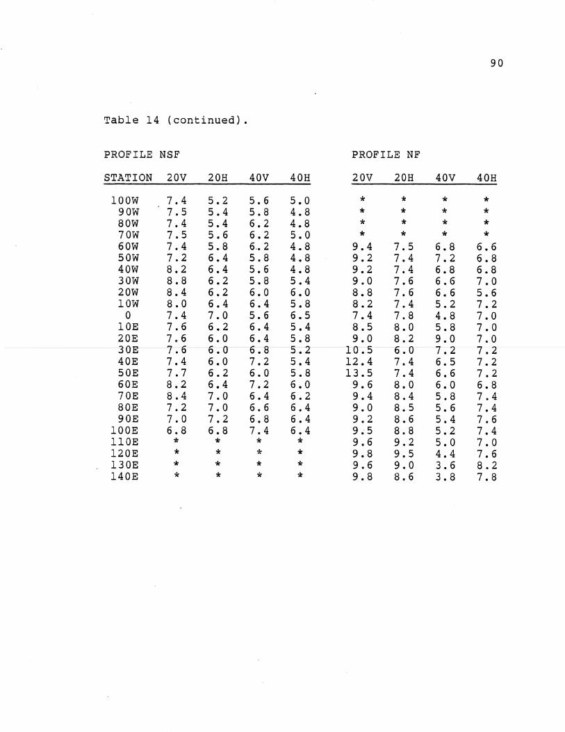
14 Electromagnetic data at Cross Bar Ranch .••••••... 89

15 Electromagnetic data at Crystal River Quarry No 2. 92

iv

LIST OF FIGURES

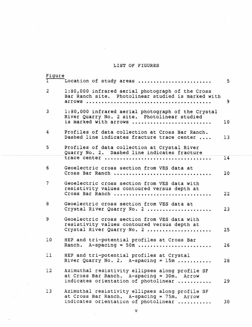
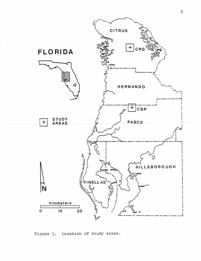
Figure 1 Location of study areas •••••••.•.....•••.•••••• 5

2 1:80,000 infrared aerial photograph of the Cross Bar Ranch site. Photolinear studied is marked with arrows ......................................... 9

3 1:80,000 infrared aerial photog~aph of the Crystal River Quarry No. 2 site. Photolinear studied is marked with arrows •••••.•.•.••••.••••.•••... 10

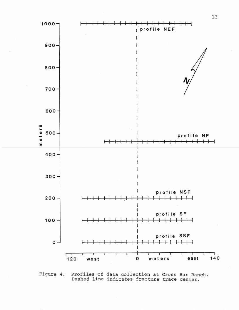
4 Profiles of data collection at Cross Bar Ranch. Dashed line indicates fracture trace center •••. 13

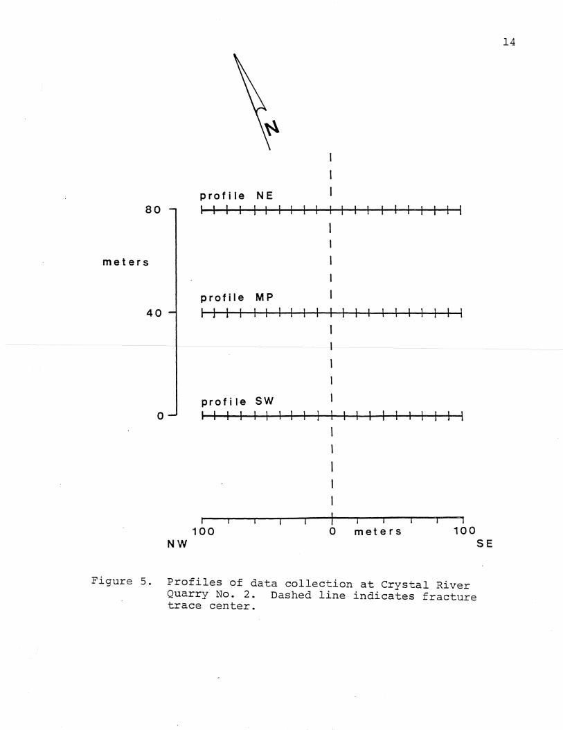
5 Profiles of data collection at Crystal River Quarry No.2. Dashed line indicates fracture trace center ................................... 14

6 Geoelectric cross section from VES data at ' Cross Bar Ranch •.••...•••..•••••...••••••.••••. 20

7 Geoelectric cross section from VES data with resistivity values contoured versus depth at Cross Bar Ranch •.•.•...••.••.•.•••••.•••••.•• •..• 22

8 Geoelectric cross section from VES data at

9

10

11

12

13

Crystal Ri ver Quarry No.2................. . . . • 23

Geoelectric cross section from VES data with resistivity values contoured versus depth at Crystal River Quarry ·No. 2 .•..•••....••...••••.

HEP and tri-potential profiles at Cross Bar Ranch. A-spacing = 50m •••..••....•••••••..••..

HEP and tri-potential profiles at Crystal River Quarry No.2. A-spacing = 15m .••....•.•.

Azimuthal resistivity ellipses along profile SF at Cross Bar Ranch. A-spacing = 30m. Arrow indicates orientation of photolinear .•.........

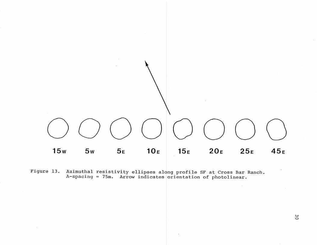
Azimuthal resistivity ellipses along profile SF at Cross Bar Ranch. A-spacing = 75m. Arrow indicates orientation of photolinear .......... .

v

25

26

28

29

30

14

15

Azimuthal resistivity ellipses along profile NE at Crystal River Quarry No.2. A-spacing = 15m. Arrow indicates orientation of photolinear .•••.

Microgravity profiles at Cross Bar Ranch •...•••

16 Vertical gravity gradient profiles at Cross Bar

32

33

Ranch •••••••••••••••••••••••.• e· • • • • • • • • • • • • • • • • 34

17 Microgravity profiles at crystal River Quarry No.2. . . . . . . . . . . . . . . . . . . . . . . . . . . . . . . . . . . . . . . . . . 35

18 Vertical gravity gradient profiles at Crystal River Quarry No.2............................. 36

19

20

21

EM profiles at Cross Bar Ranch. 20m coil spacing; vertical dipole. Conductivity values in mmhos/m •••••••••.•••••.••••••••.•.•••••.•.•.

EM profiles at Cross Bar Ranch. 40m coil spacing; vertical dipole. Conductivity values in mmhos/m .................................... .

EM profiles at Crystal River Quarry No.2. 20m

38

39

coil spacing; vertical dipole. Conduc ... t ... ~h' v",,~.;--c' t~y'-'---"---------values in mmhos/m •••...•••.••.••••..••.••.•.•.•

22 EM profiles at Crystal River Quarry No.2. 40m coil spacing; vertical dipole. Conductivity

41

values in mmhos/m .••.••...•••...••...••••.••... 42

23 Calculated gravity values and polygons approximating the limestone surface at Cross Bar Ranch .•.•..•.••••.•••..••.••••.•••..•••.••..•.. 54

24 Geologic interpretation of the Cross Bar Ranch fracture zone based on geophysical and soil boring data. Arrows indicate soil boring locations ...................................... 57

25 Geologic interpretation of the Crystal River Quarry No. 2 fracture zone based on geophysical and soil boring data. Arrows indicate soil boring locations ••.•••..•....•..•..•.•.•..•.•.. 64

vi

/

ABSTRACT

Multiple geophysical methods were used to determine the geophysical

and geologic character of fracture traces in the carbonate Floridan

aquifer. The methods used were vertical electric soundings, horizontal

electric profiles, tri-potential profiles, azimuthal resistivity

ellipses, microgravity profiles, vertical gravity gradient profiles, and

electromagnetic profiles. Two sites were studied in west-central

Florida. One site is within a municipal wellfield where the limestone is

buried beneath lO-30m of overburden and the water table is about 5-6m

below land surface. The other site is adjacent to a rock quarry where

the limestone is buried beneath lO-2Om of unsaturated overburden. The

fracture zone passes through the rock quarry and can be observed in

------,Ottt--erop. Soi 1 bori-ft"§~ere compl eted at each 5-ite----l-l+---~l"'___to_c.al i brate~~~~~­

the geophysical data.

The study demonstrates that several of the geophysical methods are

useful in characterizing the location, geometry, and stratigraphy

associated with each fracture zone. The fracture zones are defined by

resistivity lows with vertical electric soundings and horizontal electric

profiles. Tri-potential profiles exhibit major divergences in the

responses of the measured electrode configurations. The azimuthal

resistivity ellipses show a high degree of anisotropy over the fracture

zone but are difficult to interpret. The microgravity data exhibit broad

gravity lows over the fracture zone. Enhancement of the microgravity

data by vertical gravity gradient profiles does not appear to be

worthwhile because survey inaccuracies are magnified. Electromagnetic

profiles exhibit sharp conductivity highs over the fracture zones. All

of the geophysical methods exhibit variability in response along the

vii

trace, suggesting that karstic development is not uniform along the

length of the fracture zone.

The geophysical results reveal two very different subsurface

expressions. The fracture zone studied at the wellfield is marked by a

deep, V-shaped depression in the limestone which appears to have formed

through solution development along the trace. The fracture zone studied

at the quarry is underlain by a small V-shaped depression in a bedrock

ridge, which may have formed by differential weathering of recrystallized

limestone along the trace.

viii

1

INTRODUCTION

It has long been recognized that photolinears visible

on aerial photographs are linear natural-drainage,

soil-tonal, and topographic alignments which are the surface

manifestations of underlying vertical to near-vertical zones

of fracture concentration (Lattman and Parizek, 1964). The

surface expressions of fracture traces may be several

hundred meters wide, but the narrow zone of fracture

concentration within the underlying bedrock may only be 2 to

20 meters wide (parizek, 1976).

Fracture traces appear to be universal in their

distribution and are systematically oriented in four

principal directions: WNW, NNW, NNE and ENE. The

mechanisms responsible for fracture-trace formation include:

tidal stresses due to the gravitational effects of the sun

and moon; the changes in radial acceleration of the earth

along its radius vector; and, the gradual decrease in the

earth's rate of rotation due to tidal friction (Blanchet,

1957).

Many studies have established a relationship between

fracture traces and zones of increased solution, porosity

and permeability within bedrock aquifers (Lattman and

Parizek, 1964; setzer, 1966; Wobber, 1967; Siddiqui and

2

parizek, 1971; F1orquist, 1973; Parizek, 1976; Stre1tsova,

1976; LaRiccia and Rauch, 1977; Miller, 1977; LeGrand,

1979). These zones of increased hydraulic conductivity are

important in

contamination

groundwater

studies and

prospecting,

geotechnical

groundwater­

considerations.

Wells located on fracture traces or fracture-trace

intersections can have yields many times greater than those

located in interfracture areas. Fracture zones are

vulnerable to groundwater contamination and may influence

the direction of contaminant transport. The high void

ratios and cavernous porosity in fracture zones in carbonate

rocks can leac to s~nkhole cevelopment and create hazardous

foundation conditions for overlying structures.

In an effort to evaluate the geophysical responses of

fractures, cavities and potential aquifers, geophysical

surveys have been used in several investigations. Electrical

resistivity methods, which include horizontal electric

profiling (HEP), vertical electric soundings (VES), and/or

tri-potential profiling, have been used by Carpenter and

Habberjam (1956), Johnson (1966), Habberjam (1969), Smith

and Randazzo (1975), Kirk (1976), and Ogden and Eddy (1984).

Leonard-Mayer (1984) and Taylor (1984) have used azimuthal

resistivitysurveys to determine joint orientations and

joint porosity in near-surface formations. Moore and

Stewart (1983) have integrated VES, seismic refraction and

microgravimetry in characterizing the geophysical signatures

3

of fracture traces. Gravity surveys to detect subsurface

voids have been performed by Arzi (1975), Fajklewicz (1976),

Hammer (1970), Omnes (1975), Thyssen-Bornemisza (1965), and

others, however, only Moore and stewart's study has been

devoted to fracture traces.

The objective of this study is a comparative analysis

of several geophysical methods to precisely locate the

narrow zone of fracture concentration within fracture traces

observed on aerial photographs in west-central Florida. The

geophysical methods used are VES, HEP, tri-potential

resistivity profiles, azimuthal resistivity, microgravity

prof~Ies, vertical gravity gradient profiles, and EM

profiles. On-site soil borings and outcrop observations are

used to calibrate the geophYSical data and aid in the

comparison and interpretation of each method.

The geophysical data, soil borings and outcrop

observations are used to determine the general physical

characteristics of fracture zones by mathematical modeling.

The fracture zone properties such as bulk density, width, .

effect of overlying sediments, and contrast with

inter fracture zones determined from the mathematical models,

allow for a greater understanding of the geologic character

of fracture traces in west-central Florida.

4

SITE LOCATIONS

The study was conducted at two sites in west-central

Florida (Figure 1). The first site is the Cross Bar Ranch

Wellfield located approximately 41 km north of Tampa,

Florida in northern Pasco County. The survey area across

the trace is in NW 1/4 Sec 12, Twn 24, Rng 18. The land is

used primarily for cattle grazing and farming. Relief is

generally less than a few meters. Cross Bar Ranch lies in

-----------+e-ne-Coa-s-tai-P1.crtn Prov1.~nc_e-crf-Flm!l--eman ( :t!t28) , and on en:e

Wicomico terrace of the Terraced Coastal Lowlands of Vernon

(1951) •

The second site includes the Crystal River Quarry No.

2 and the adjacent cattle pasture to the south. The quarry

is about 3 km

County. The

south of Lecanto, Florida in cen~ral Citrus

quarry is an active limerock mine producing

crushed and graded stone. The survey area across the trace

is in NW 1/4 Sec 22, Twn 18, Rng 18. The pasture is used

for cattle grazing and exhibits several meters of relief.

crystal River Quarry No. 2 also lies in the Coastal Plain

Province of Fenneman (1928) and on the Tertiary Highlands of

Vernon (1951).

5

CITRUS

FLORIDA

- I --

I

__ J, I

I J

I I

I I

I I

N I I

I kilometers I

I o 15 30 ... I

-------______ J

Figure 1. Location of study areas.

6

HYDROGEOLOGY

The principal aquifer at Cross Bar Ranch is the

Floridan aquifer which consists of Eocene to Miocene

limestones and dolostones; the Avon Park Limestone, the

Ocala Group, Suwannee Limestone and the Tampa Limestone

(Cherry et al., 1970). A thick, residual clay separates the

Tampa Limestone and the Suwannee Limestone

and partially confines the Floridan aquifer.

in some places

Overlying the

thick carbonate units is a sequence of Pliocene to Holocene

unconsolidated sands, silts, and sandy silts and clays which

form the surficial aquifer and vary from a-30m in thickness.

The water table in the surficial aquifer lies approximately

5-6m below land surface.

The principal aquifer at Crystal River Quarry No.2

also is the Floridan aquifer, consisting of the Avon Park

Limestone and the Ocala Group. Occurrences of the Suwannee

Limestone are scattered, capping only the higher hills,

while the Tampa Limestone is absent in this area. Overlying

the carbonate units is a sequence of Pliocene to Holocene

unconsolidated sands and sandy clays. The Floridan aquifer

is generally unconfined and the water table is a few meters

below the top of the limestone, except where perched above

the sandy clays.

7

The vertical and horizontal permeabilities of

the carbonate units are influenced by the amount and

intensity of fracturing and solution development of the

carbonate bedrock. Hard, competent bedrock is often subject

to abundant fracturing and jOinting, along which develop

zones of increased solution activity. These openings

provide an avenue of increased groundwater flow, both

laterally and vertically. Many of these vertical fractures

extend upward through the limestone and are expressed at the

surface as shallow depressions, linear-swales, sinks, and

soil-tonal patterns (Moore and stewart, 1983).

8

FRACTURE ZONE IDENTIFICATION

The fracture trace studied at Cross Bar Ranch was

identified previously and was

stewart's (1983) investigation.

the subject of

The fracture

Moore

trace

and

was

chosen for this study for its known characteristics, which

provide additional control for geophysical correlation. The

photolinear is easily identified on 1:80,000 infrared and

1:20,000 black and white stereo-paired aerial photographs as

a light gray, linear, soil-tonal pattern striking N27 0 W,

extend~ng about 1.5 km ~n length and 0.2 km ~n w~dth (F~gure

2). The trace is located in the field by a gentle linear

swale with up to 2m of relief. Small patches of oak trees

are commonly aligned and sit in depressions on the trace.

The fracture trace studied at Crystal River Quarry No.

2 was chosen because the fracture zone is observable in

outcrop in the quarry walls. This also provides control for

geophysical interpretation. From 1:80,000 infrared and

1:20,000 black and white, stereo-paired aerial photographs

the photolinear is identified as a dark gray, linear,

soil-tonal pattern striking N2SoE, extending about 2-3 km in

length and 0.1 km in width (Figure 3). In the field, the

trace is easily located by a linear swale with up to 6m of

relief. Looking across the mine pit, along the trace, the

11

tree line on the opposite quarry wall dips in the center of

the trace. The trace is observed in outcrop as a zone of

hard, recrystallized limestone with soft, weathered

limestone to either side. The fracture zone is inconsistant

from outcrop to outcrop, but is recognized by a high

frequency of fracturing or a zone of vertical, clay-filled

fractures.

12

GEOPHYSICAL METHODS AND DATA COLLECTION

The geophysical data were collected along multiple

profiles oriented perpendicular to the fracture traces at

both Cross Bar Ranch and Crystal River Quarry No.2. The

center of each fracture trace was located in the field using

aerial photographs and topographic maps, and by observing

land surface relief. The center of each profile was located

on the trace and marked as station zero (0). 'Stations along

each profile 'were labled as east or west from the center of

the profile in meters (Figures 4 and 5). The field data

were collected from May 1984 through January 1985 using a

SR-50 Soiltest resistivity meter, Worden Master Gravimeter

number 1022, and a Geonics 34-3 terrain conductivity meter.

Soil borings were completed at selected sites by a sub-

contracted soils testing company.

Vertical Electric Soundings

At Cross Bar Ranch, VES were completed at nine stations

along profile SF. Eleven VES were made at Crystal River

Quarry No. 2 along profile NE and two were made along

profile SW. The VES were made parallel to the fracture

trace using the Wenner 'electrode configuration (Telford et

al., 1976) with A-spacings ranging from 1 to 160 meters.

1000

900

800

700

600

Q) 500 -Q)

E

400

300

200

100

o

I i

120

I I I I I I I I I I I I I I I I I I I profile NEF

profile NF

I I I I I I I I I I I I I I I I I I I I -----1-

profi Ie NSF I I I I I I I I .1 I I I I I I I I I I

I I I I I I I I I I

west o

profi Ie SF 1 I I I I I I I I

profile SSF I I I I I I I

I I meters east

Figure 4. Profiles of data collection at Cross Bar Ranch~ Dashed line indicates fracture trace center.

13

140

profile NE 80 I I I I I I I I I I I I I I I I I I I I

meters

profile MP

40 I J I I I I I I I I 1 I I I I I 1 I I I

I

profi Ie SW I o I I I I I I I I I I I I I I I I I I I I I

I

i 100

NW

I I

I i o meters 100

SE

Figure 5. Profiles of data collection at Crystal River Quarry No.2. Dashed line indicates fracture trace center.

14

15

The apparent resistivities calculated in the field were

automatically reduced to geoelectric layers using an

inversion program developed by Zhodyand Bisdorf (1975).

The inversion program provides calculated depth, thickness,

and bulk resistivity values for each layer in the

geoelectric section. Geologically unreasonable or thin

units are adjusted by combining geoelectric layers of

similar bulk resistivity until the final solution consists

of fewer than five or six layers. Geoelectric cross

sections were constructed using these reduced solutions and

contours of resistivity for distance versus depth were

constructed.

Horizontal Electric and Tri-Potential Profiles

Five HEP and tri-potential profiles were completed at

Cross Bar Ranch with a 10m station spacing. Two HEP and

tri-potential profiles were completed at Crystal River

Quarry No. 2 with stations occupied every Sm. The

tri-potential method involves three different electrode

configurations; the standard Wenner (CPPC) used for HEP, a

dipole-dipole (CCPP), and a bipole-bipole (CPCP), using a

fixed A-spacing for all three. Apparent resistivity was

measured at each station for each electrode configuration.

HEP's reveal lateral differences in bulk resistivity of the

geoelectric section, while tri-potential profiles detect

vertical discontinuities through apparent resistivitiy

16

variations between the three array configurations (Ogden and

Eddy, 1984).

these data.

Multi-profile plots were constructed using

Azimuthal Resistivity

Sixteen azimuthal resistivity stations were occupied at

Cross Bar Ranch and thirteen at Crystal River Quarry No.2.

The azimuthal method uses the Wenner array with a fixed

A-spacing which is rotated through 360 0 at 30 0 increments to

determine the dependance of resistivity on the orientation

of the electrode array. At Cross Bar Ranch, A-spacings of

30m and 7Sm were used while at Crystal River Quarry No.2 an

A-spacing of 15m was used. The azimuthal resistivity method

is sensitive to the orientation and intensity of jOint sets

(Leonard-Mayer, 1984). Resistivity ellipses were

constructed using these azimuthal data.

Microgravity and Vertical Gradient of Gravity Profiles

Two hundred and thirty-four gravity stations were

occupied at Cross Bar Ranch and two hundred and forty-six

gravity stations were occupied at Crystal River Quarry No.2

with readings taken every Sm across the trace. The field

procedure was similar to the looping method described by

Nettleton (1940). Base stations were occupied every 30-60

minutes with an instrument and tidal drift of less than 0.15

mgal per hour. Elevation was controlled to + 0.0031m by

leveling with a transit and stadia rod. The field data were

17

reduced to simple Bouguer anomaly values using standard

procedures as described in Parasnis (1966) and Telford et

ale (1976). A Bouguer density of 2.0 g/cc3 was used in the

corrections. Gravity readings were taken on three parallel

profiles separated by Sm. It was possible to calculate the

vertical gradient of gravity from the triple track data

using a method described by Thyssen-Bornemisza (196S)

because it follows the Laplace equation. Microgravity

surveys measure gravity anomalies of 10-1 mgals, as compared

to anomalies of 100-101 mgals in standard gravity surveys.

The vertical gradient of gravity tends to accentuate near

surface features at the expense of deeper ones.

Microgravity and vertical gradient of gravity profiles were

constructed using the reduced gravity values.

Electromagnetic Profiles

One hundred and five EM stations were occupied at Cross

Bar Ranch and sixty-three EM stations were occupied at

Crystal River Quarry No.2. EM measurements were taken

every 10m with coil separation distances of 10, 20 and 40

meters. The instrument allows for a direct reading of

terrain conductivity which is a function of the secondary

magnetic field strength, intercoil separation, and operating

frequency. The effective depth of exploration is a function

of coil spacing (s) and orientation. For vertical dipoles

the effective depth is 15, 30 and 60 meters (l.Ss) and for

18

horizontal' dipoles the effective depth is 7.5, 15 and 30

meters (0.75s; McNeill, 1980). The resulting terrain

conductivity readings represent bulk conductivity values and

are sensitive to lateral differences in the measured

geoelectric section. Multi-profile plots for similar coil

spacings and dipole orientations were constructed using

these data.

Soil Borings

Two exploratory soil borings were drilled at Cross Bar

Ranch along profile SF at stations 80W and 30E. Three soil

borings were drilled along profile NE at Crystal River

------\itQI.la-~~:y__No_.-2----a-t-s-ta-t-i0n-s-----'7-2-NW-,----5-O-NW---an-G-1-5NW • 'I'-h e bo-!"-i-~s------

penetrated the unconsolidated deposits and extended into the

lifflestone bedrock. Each major lithologic unit was sampled

with a split spoon coring tool and the sediment was analyzed

for percentage of sand, silt and clay by wet sieve and

hydrometer.

19

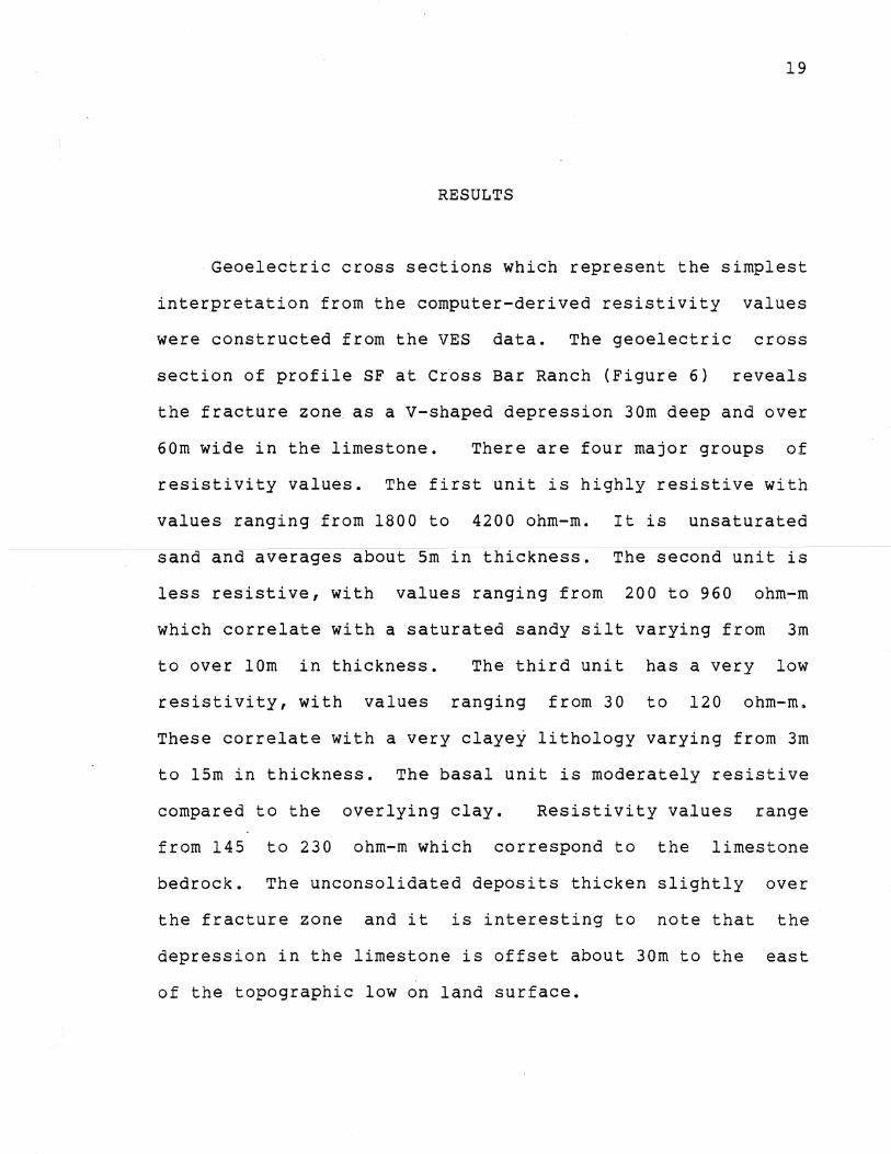
RESULTS

Geoelectric cross sections which represent the simplest

interpretation from the computer-derived resistivity values

were constructed from the VES data. The geoelectric cross

section of profile SF at Cross Bar Ranch (Figure 6) reveals

the fracture zone as a V-shaped depression 30m deep and over

60m wide in the limestone. There are four major groups of

resistivity values. The first unit is highly resistive with

values ranging from 1800 to 4200 ohm-me It is unsaturated -- -

sand and averages about 5m in thickness. The second unit is

less resistive, with values ranging from 200 to 960 ohm-m

which correlate with a saturated sandy silt varying from 3m

to over 10m in thickness. The third unit has a very low

resistivity, with values ranging from 30 to 120 ohm-me

These correlate with a very clayey lithology varying from 3m

to 15m in thickness. The basal unit is moderately resistive

compared to the overlying clay. Resistivity values range

from 145 to 230 ohm-m which correspond to the limestone

bedrock. The unconsolidated deposits thicken slightly over

the fracture zone and it is interesting to note that the

depression in the limestone is offset about 30m to the east

of the topographic low on land surface.

0 I 2355

248

51

1°i-. 168 en ....

_--------3274 902 __ 2624

__________ -J. 1820 64 ------ 2216 3700 3.42 3084

581 -....:. 399 ............ -/---/--__ 487 --

151 55

372

206 229 Q) 10.6 -Q)

E 20

c

.c -a. Q)

"0 30

,-;:\ 8'

: '~~ __ J-

115

227

)

60 -146

120

40

_/202

158

r-- I I, I I I I 80 west 0 meters east 80

I

Figure 6. Geoelectric cross section from VES data at Cross Bar Ranch. Apparent resistivities are given in ohm-meters; heavy lines are control points from soundings.

420('

-961

-29 -170

tv o

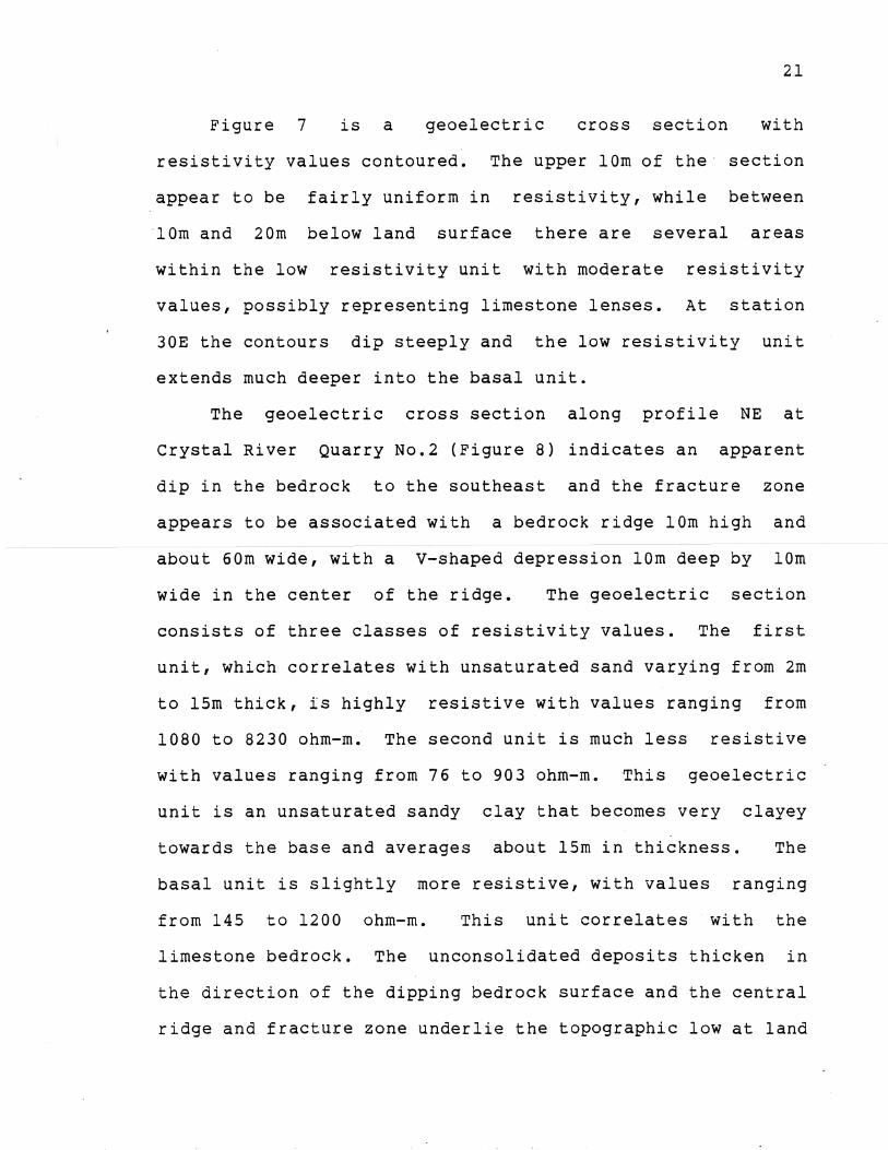
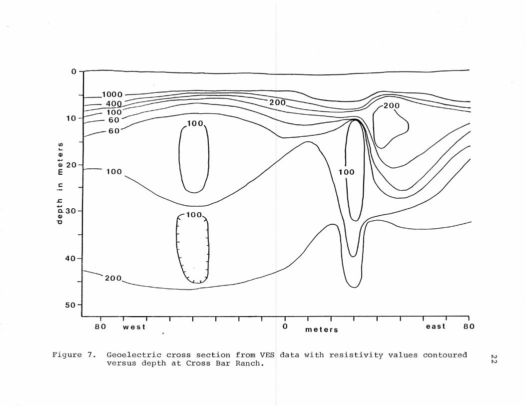
21

Figure 7 is a geoelectric cross section with

resistivity values contoured. The upper 10m of the section

appear to be fairly uniform in resistivity, while between

"10m and 20m below land surface there are several areas

within the low resistivity unit with moderate resistivity

values, possibly representing limestone lenses. At station

30E the contours dip steeply and the low resistivity unit

extends much deeper into the basal unit.

The geoelectric cross section along profile NE at

Crystal River Quarry No.2 (Figure 8) indicates an apparent

dip in the bedrock to the southeast and the fracture zone

appears to be associated with a bedrock ridge 10m high and

about 60m wide, with a V-shaped depression 10m deep by 10m

wide in the center of the ridge. The geoelectric section

consists of three classes of resistivity values. The first

unit, which correlates with unsaturated sand varying from 2m

to 15m thick, is highly resistive with values ranging from

1080 to 8230 ohm-me The second unit is much less resistive

with values ranging from 76 to 903 ohm-me This geoelectric

unit is an unsaturated sandy clay that becomes very clayey

towards the base and averages about 15m in thickness. The

basal unit is slightly more resistive, with values ranging

from 145 to 1200 ohm-me This unit correlates with the

limestone bedrock. The unconsolidated deposits thicken in

the direction of the dipping bedrock surface and the central

ridge and fracture zone underlie the topographic low at land

°ll----------------------------t----------------------------

10

If) L-

a> -a> 20 E r-100

c:

.c -a. 30 a> "0

40

200

50

meters

Figure 7. Geoelectric cross section from VESI data with resistivity values contoured versus depth at Cross Bar Ranch.

tv tv

o

10 o ... Q)

+-' Q)

E 20

c

30

.c +-' a. Q)

"C

40

I

I j

I !

I _____

- J 309. 8232 1514 ..... __ --

--------- 898 4272 _~ 5954 5070 5750~-"-...4297 1081 _/' I

-- ---~ 2132

------ I .95 __ 4.43 9p3 ___ 176 j 243 76 343 I'

134 329 -, /165

170""_............... /456 172 ~_~

146 -154

237 _--I 347

'3i68 1197

308

'-151

862

170

I

I 154 I -

I --T I I I I I I I 80 NW 0 I meters SE 100

I

Figure 8. Geoelectric cross section ~pparent resistivities are paints from soundings.

from VES 1ata at Crystal River Quarry No.2. given in {hm-meters; heavy lines are control

!

N W

24

surface. The resistivities of the limestone unit are higher

on the ridge than on either side of it. Along the ridge the

resistivities are 160 to 1200 ohm-m, while on either side

they range from 150 to 340 ohm-me

Figure 9 is a geoelectric cross section at Crystal

River Quarry No. 2 with the calculated resistivity depth

values contoured. The upper 10m of the geoelectric section

are relatively uniform in resistivity. At stations 80W and

60E small ·pockets n of very low resistivity exist about 15m

below land surface. Between stations 30W-20W and 10E-20E,

there are slightly larger ·pockets· of low resistivity that

dip toward the trace center. At the trace center, the 200

---------~-- ohm-m--contour extends over 15m into the

moderate-resistivity, basal unit.

The HEP and tri-potential plots at Cross Bar Ranch

(Figure 10) indicate low resistivity values for the CPPC

array (HEP) at 40E and 90E on profile SSF, at 20E on profile

SF and at 40W and 70E on profile NSF. These low resistivity

values represent some lateral difference in bulk resistivity

of the measured geoelectric section and appear to be fairly

consistent between stations 20E and 75E of the profiles.

The tri-potential profiles reveal sharp divergences in the

resistivity values measured by the CPPC and the CPCP arrays

between stations 20E and 75E, indicating an electrical

discontinuity or vertical fracture (Ogden and Eddy, 1984).

A divergence of the tri-potential arrays is also observed

-------o ---------------

10

II) ... Q)

+-' Q) 20 E c:

..c: 200 +-' a. 30 Q)

"0

40

80 NW o meters SE

Figure 9. Geoelectric cross section from VES data with resistivity values contoured versus depth at Crystal River Quarry No.2.

80

N Ul

240

profile NSF

ohm-m

120 240

profile SF

ohm-m --~ -~-------~------~~-f\

120

220

profile SSF

ohm-m

o-cppc o-cpcp Cl-ccpp

120+---r--'--~--~--r--.--~--~--~~

west 100 o 100

meters

Figure 10. HEP and tri-potential profiles at Cross Bar Ranch. A-spacing = SOme

26

east

27

between 30W-40W on profile NSF and may indicate an isolated

fracture.

The HEP and tri-potential plots at Crystal River Quarry

No.2 (Figure 11) indicate a strong resistivity low along

profile NE in the CPPC configuration (HEP), with the lowest

value about 13m southeast of the central depression of the

trace. Along profile SW, little resistivity contrast is

observed in the CPPC configuration (HEP). The tri-potential

survey along both profiles indicate divergences on each

profile. Divergences are observed at stations 77NW, 12NW

and 12SE on profile NE, and at stations 52NW, 17SE and 42SE

on profile SW. The di&t~n£es between stations of divergence

are equal on both profiles indicating a linear relationship

at some orientation other than the strike of the

photolinear.

Azimuthal resistivity ellipses were constructed

along profile SF at Cross Bar Ranch with Wenner A-spacings

of 30m and 75m •. The 30m A-spacing ellipses (Figure 12) are

almost iso~ropic to the west of the trace center, but to the

east, anisotropy of the ellipses is high over the v-shaped

depression of Figure 6. A rotation of nearly 90 0 of the

orientation of the major axes of the ellipses is observed

from stations 0 to 60E. The 75m A-spacing ellipses (Figure

13) are all nearly isotropic, except at station 15E, which

has a resistivity low in the same azimuth as the strike of

the fracture trace.

1000

E

E ~ o

100 profile NE

1000

E I

E

100

80

NW

o-cppc o-cpcp c:;;-ccpp

o meters

28

50

SE

Figure 11. HEP and tri-potential profiles at Crystal River Quarry No.2. A-spacing = 15m.

0000 60w

Figure 12.

I

40w 20w 0 20F 30E 40E 50E I

Azimuthal resistivity ellipses aling profile SF at Cross Bar Ranch. A-spacing = 30m. Arrow indicates I orientation of photo1inear.

60E

tv 1.0

00000000 15w

Figure 13.

5w

Azimuthal A-spacing

5E 10E 15E 20E 25E

I

resistivity ellipses aldng profile SF at Cross Bar Ranch. = 75m. Arrow indicates I orientation of photolinear.

45E

w o

31

At Crystal River Quarry No.2, azimuthal resistivity

ellipses were constructed along profile NE using Wenner

A-spacings of 15m (Figure 14). These ellipses show a high

degree of anisotropy and the relative resistivity decreases

over the center of the trace. The azimuths of the major axes

of the ellipses appear to rotate 90 0 from stations 42NW to

12SE. stations 2NW, 22SE and 32SE show the highest degree

of anisotropy, with resistivity lows that pinch the ellipses

indicating the strike of some less resistive linear unit.

The microgravity profiles SF and NF at Cross Bar Ranch

(Figure 15) both show a sharp, strong gravity low of about

0.2 mgal east of the trace center, corresponding to the ------ --- -- -

location of the V-shaped depression of Figure 6. The second

vertical derivatives of gravity calculated from triple-track

profiles over the same stations are shown in Figure 16. The

same general patterns as the microgravity profiles are

observed, but the station-to-station gradients of gravity

values are considerably noisier.

Figure 17 illustrates microgravity profiles SW and NE

at Crystal River Quarry No.2. Profile SW is fairly noisy

and the fracture zone shows little gravity response.

Profile NE shows a gravity low of about 0.2 mgal about 20m

east of the trace center. Both profiles show gravity values

which decrease to the southeast, corresponding to the

dipping bedrock surface (Figure 8). Second vertical deriva-

tives of gravity values at the same stations (Figure 18)

00 OO()PO o 92 72 52 42 32 22 12 2 12 22 32 60 100

Northwest

Figure 14.

Southeast

Azimuthal resistivity ellipses altng profile NE at Crystal River Quarry No.2. A-spacing = 15m. Arrow indicates orientation of photolinear.

Lv N

190.80

profile NF

190.70

mgals

190.60

profile SF

184.70

mgals

184.60

100 west

(

o mete rs

Figure 15. Microgravity profiles at Cross Bar Ranch.

33

140 east

+0.01

profile NF

0.0

mgal/m 2

-0.01

+0.01

profile SF

0.0

mgal/m 2

- 0.01

100 west

o meters

34

140 east

Figure 16. Vertical gravity gradient profiles at Cross Bar Ranch.

35

176.70

profile NE

176.60

mgals

176.50

-----------~7~·~~-------------------------------------------~-----------

178.00

profi Ie ·SW

177.90

mgals

177.80

177.70

NW

I 100

I o

meters 100

SE

Figure 17. Microgravity profiles at Crystal River Quarry No.2.

36

+ 0.01

profile NE

0.0

mgal/m 2

------------~~or.ol_~------------------------------------~-~+---------------------

+0.01

profile SW

0.0

mgal/m 2

- 0.01

100 o 100 SE NW meters

Figure 18. Vertical gravity gradient profiles at Crystal River Quarry No.2.

37

again show similar responses, but are considerably noisier

than the microgravity profiles.

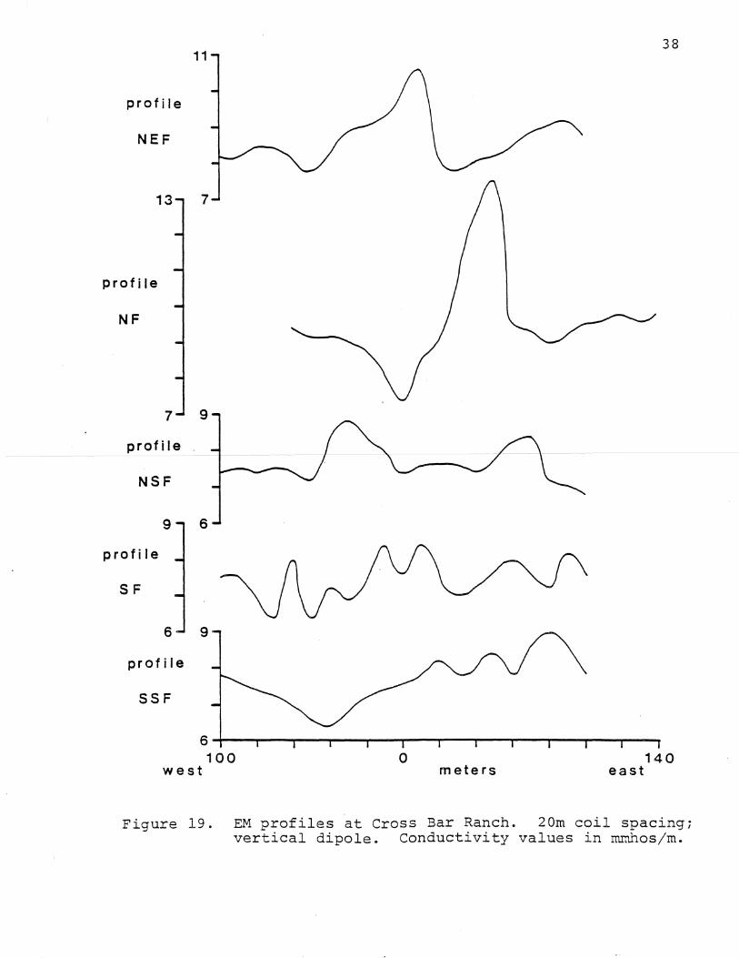
Electromagnetic coil spacings of 20m and 40m for both

horizontal and vertical dipoles were occupied at each

station along profiles SSF, SF, NSF, NF and NEF at Cross Bar

Ranch. The influence of the fracture zone is not detected

by the shallow depth of investigations produced by the 20m

and 40m horizontal dipoles. The multiple profiles of the

20m vertical dipole survey (Figure 19), where 70 percent of

the response is from materials less than 30m deep, show

distinct conductivity highs of up to 4 mmhos/m over

background. Peaks occur at station 50E along profile NF and --- --- --- --------

10E along profile NEF. The profiles located

further to the south show little significant contrast of

terrain conductivity.

The multiple profiles of the 40m vertical dipole survey

(Figure 20), where 70 percent of the response is from

materials less than 60m deep, reveal obvious conductivity

highs of up to 3 mmhos/m over background along three of the

five profiles. Profile SSF is marked by a broad

conductivity high, with a peak at station 20E. The profiles

located to the north, NF and NEF, both show sharp anomalies

at station 20E, while profiles SF and NSF reveal little

contrast in conductivity. When all the EM profiles are

correlated, a conductivity high due to the fracture zone is

38 11

profile

NEF

13 7

profile

NF

7 9

profile

NSF

9 6

profi Ie

SF

6 9

profile

SSF

6 100 0 140

west meters east

Figure 19. EM profiles at Cross Bar Ranch. 20m coil spacingi vertical dipole. Conductivity values in mrnhos/m.

39 9

prof i Ie

NEF

9 5

profile

NF

8

3 profile

NS F

6 5 profi Ie

SF

4 8

profile

SSF

3+---~~---r--~--r-~--~--T---~~-------100

west o

meters 140

east

Figure 20. EM profiles at Cross Bar Ranch. 40m coil spacingi vertical dipole. Conductivity values in mmhos/m.

40

apparent. The location of the anomaly varies from profile to

profile, but consistently lies between stations 10E and SOE.

At Crystal River Quarry No.2, EM coil spacings of 10m,

20m and 40m for both horizontal and vertical dipoles were

occupied at each station along profiles SW, MP and NE.

Again, the shallow depth investigations of the 10m

horizontal and vertical dipoles, and the 20m horizontal

dipole do not show any significant response due to the

fracture zone. The 20m vertical dipole survey reveals

several anomalies along each profile (Figure 21). Profile

SW shows two, broad, conductivity highs of over 2 mmhos/m at

stations 40NW and 20SE. Profile MP has conductivity highs of

about 1 mmhos/m at stations 0 and 40SE. Along profile NE,

three conductivity highs of about 2 mmhos/m are observed at

stations 20NW, lOSE and SOSE.

The 40m vertical dipole survey (Figure 22) has the

least variability in inter-station conductivity readings and

shows the most distinct anomalies. Profile SW shows two,

broad, conductivity highs of over 4 mmhos/m that correspond

well with the anomalies in the 20m vertical dipole survey.

Profile MP shows three, small, conductivity highs of about

1.S mmhos/m, two of which correspond well with the anomalies

of the 20m vertical dipole survey, the other is between

stations 40NW and 20NW. Along profile NE, three

conductivity highs exist, but the high at station 10E is

only about 0.75 mmhos/m above background. When all the EM

Q) -.... -o ... c.

12

w z·

Q)

-o ... c.

12

o

3 (J)

Q)

-o ... c.

o

o~--~--~--~--~--~--~--~--~--~--~ 100

west o 100

mete rs east

Figure 21. EM profiles ·at Crystal River Quarry No.2. 20m coil spacingi vertical dipole. Conductivity values in mrnhos/m.

41

a.. :i

Go) --0 -. c.

12

0

w z

-o -. c.

3: U)

Go)

-0 -. c.

14

0

12

o~--~--~--~--~--~--~--~--~--~--~ 100

west o 100

meters east

Figure 22. EM profiles at Crystal River Quarry No.2. 40m coil spacing; vertical dipole. Conductivity values in rnmhos/m.

42

43

profiles are correlated, three anomalies tend to align with

peaks between 40W and 30W, a and 20E, and SOE and 60E.

Soil borings were conducted at Cross Bar Ranch along

profile SF at stations 80W (Table 1) and 30E (Table 2). The

near-surface lithology obtained from the dril~ing

corresponds well with the VES of Figure 6 although scattered

lenses of the Tampa Limestone were encountered about 8m

below land surface at station 30E. This unit appears to be

thin and discontinuous and pinches out close to the northern

boundary of the we1lfie1d (Gilboy and Moore, 1982). It

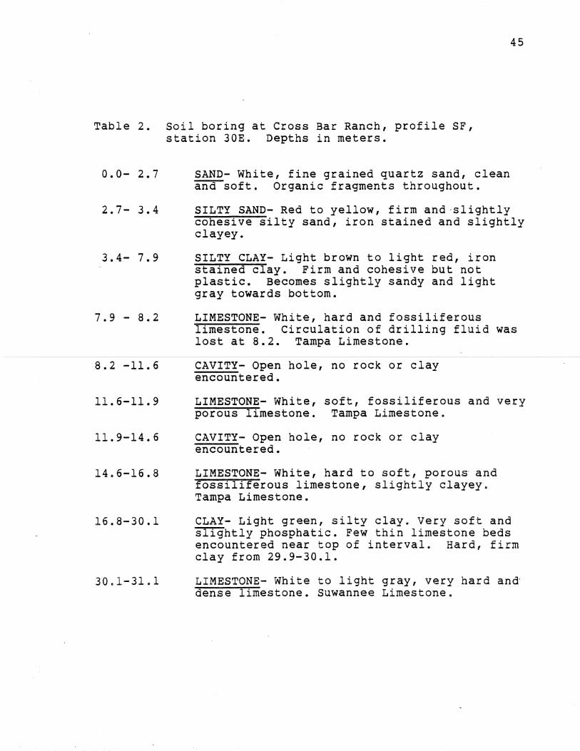
should be noted from Table 2 that unusually large fractures

or cavities were encountered in the Tampa Limestone at 30E

and a clay about 13.Sm thick was penetrated beneath it. The

Suwannee Limestone was encountered at a depth of 30m.

Three soil borings were drilled at Crystal River Quarry

No.2 along profile NE at stations 72NW (Table 3), SONW

(Table 4) and lSSE (Table S). The lithology here

corresponds well with the VES of Figure 8 except at station

72NW where limestone ledges and abundant fragments were not

encountered until a depth of 34.Sm below land surface, and

at station lSSE where hard limestone was encountered at a

depth of 28m. Table 6 shows percent sand, silt and clay for

each major unconsolidated unit at both Cross Bar Ranch and

crystal River Quarry No~ 2.

Table 1. Soil boring at Cross Bar Ranch, profile SF, station 80W. Depths in meters •

. 0.0 - 2.4 SAND- White to light yellow, fine grained quartz sand. Slightly silty with abundant organic fragments.

2.4 - 4.4 SANDY SILT- Light gray to white sandy silt, very stiff and slightly clayey.

4.4 - 8.5 SILTY CLAY- Light brown to red, iron stained silty clay. Soft to stiff becoming very clayey towards bottom.

8.5 -10.0 LIMESTONE- White, hard limestone. Tampa Limestone.

44

45

Table 2. Soil boring at Cross Bar Ranch, profile SF, station 30E. Depths in meters.

0.0- 2.7 SAND- White, fine grained quartz sand, clean and soft. Organic fragments throughout.

2.7- 3.4 SILTY SAND- Red to yellow, firm and·slightly cohesive silty sand, iron stained and slightly clayey.

3.4- 7.9

7.9 - 8.2

8.2 -11.6

11.6-11.9

11.9-14.6

14.6-16.8

16.8-30.1

30.1-31.1

SILTY CLAY- Light brown to light red, iron stained clay. Firm and cohesive but not plastic. Becomes slightly sandy and light gray towards bottom.

LIMESTONE- White, hard and fossiliferous limestone. Circulation of drilling fluid was lost at 8.2. Tampa Limestone.

CAVITY- Open hole, no rock or clay encountered.

LIMESTONE- White, soft, fossiliferous and very porous limestone. Tampa Limestone.

CAVITY- Open hole, no rock or clay encountered.

LIMESTONE- White, hard to soft, porous· and fossiliferous limestone, slightly clayey. Tampa Limestone.

CLAY- Light green, silty clay. Very soft and slightly phosphatic. Few thin limestone beds encountered near top of interval. Hard, firm clay from 29.9-30.1.

LIMESTONE- White to light gray, very hard and dense limestone. Suwannee Limestone.

46

Table 3. Soil boring at Crystal River Quarry No.2, profile NE, station 72 NW. Depths in meters.

0.0 - 3.1 SAND- White to light yellow, medium grained quartz sand, slightly silty and clean.

3.1 - 6.2 SANDY SILT- Red to yellow, firm and slightly cohesive sandy silt. Minor limestone fragments start at 4.9 but are not continuous.

6.2 -15.5 SILTY CLAY- Light yellow to light brown silty clay with abundant white streaks. Very stiff and cohesive. Limestone fragments encountered at 15.2 but are not continuous.

15.5-32.0 CLAY- Cream to light brown clay with abundant white streaks throughout. Soft and cohesive but not very plastic.

32.0-33.2 CLAY- As above but limestone fragments are very abundant. No hard rock encountered.

33.2-34.4 CLAY- Dark brown clay, peaty and organic, very plastic and sticky.

34.4-34.7 LIMESTONE- White to buff, hard and dense limestone. Crystal River Formation.

34.7-40.8 LIMESTONE- Cream to buff, soft and weathered limestone. very clayey but not plastic. Crystal River Formation.

47

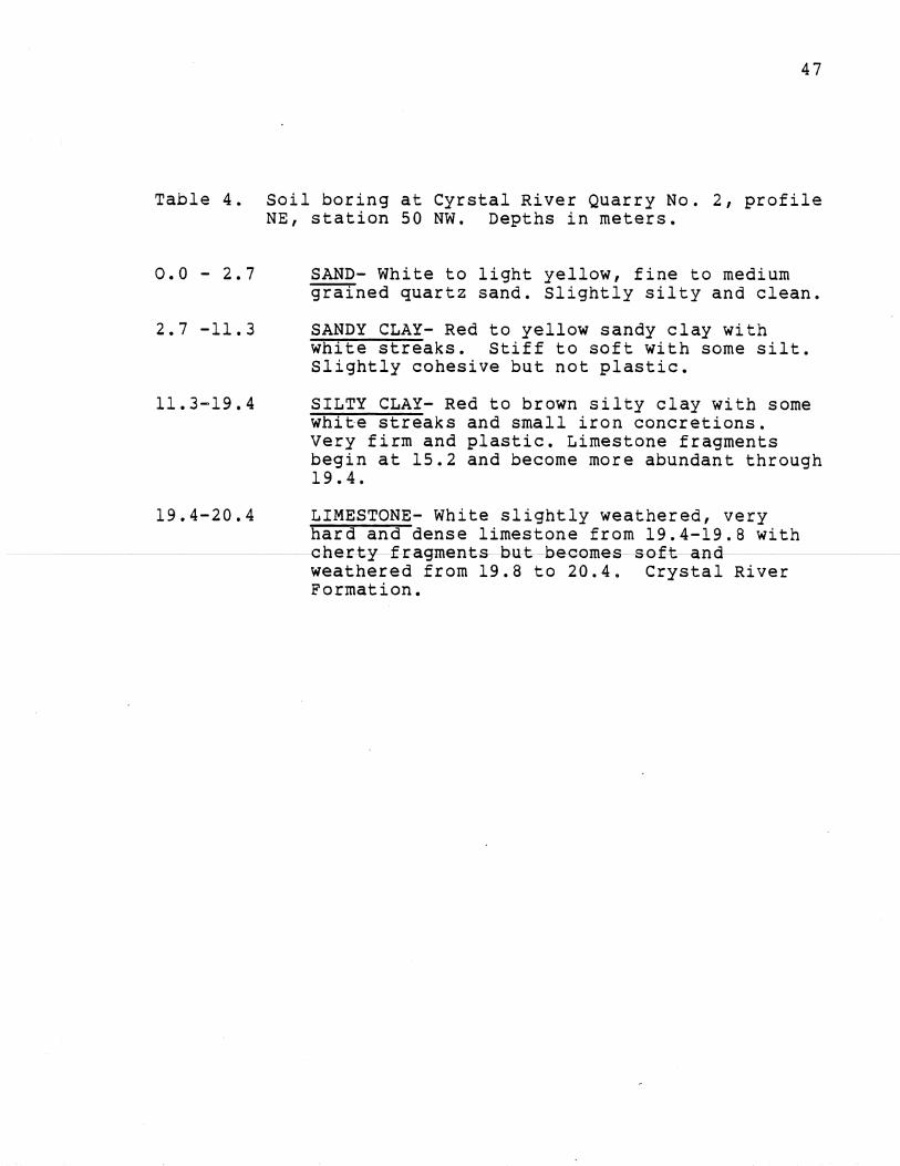
Table 4. Soil boring at Cyrstal River Quarry No.2, profile NE, station 50 NW. Depths in meters.

0.0 - 2.7 SAND- White to light yellow, fine to medium grained quartz sand. Slightly silty and clean.

2.7 -11.3 SANDY CLAY- Red to yellow sandy clay with white streaks. Stiff to soft with some silt. Slightly cohesive but not plastic.

11.3-19.4 SILTY CLAY- Red to brown silty clay with some white streaks and small iron concretions. Very firm and plastic. Limestone fragments begin at 15.2 and become more abundant through 19.4.

19.4-20.4 LIMESTONE- White slightly weathered, very hard and dense limestone from 19.4-19.8 with

--------------------~Q~~~~~~&-seeG~s-s~&-an~I-----------­weathered from 19.8 to 20.4. Crystal River Formation.

48

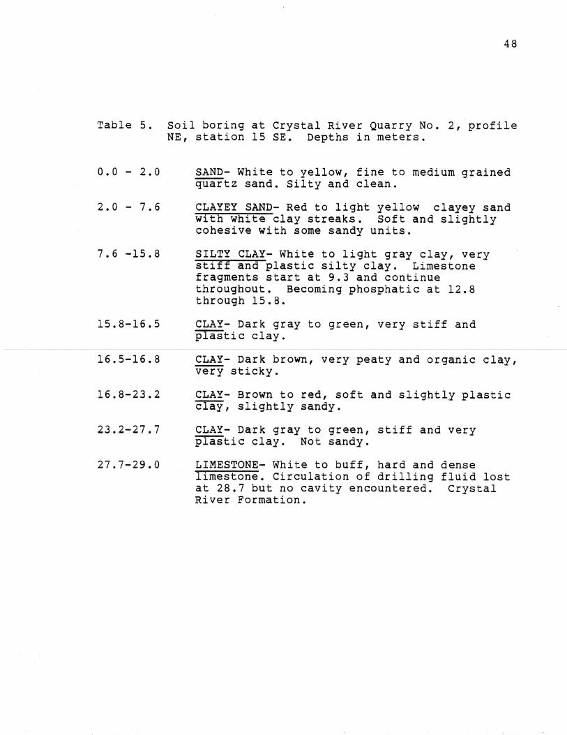
Table 5. Soil boring at Crystal River Quarry No.2, profile NE, station 15 SEe Depths in meters.

0.0 - 2.0 SAND- White to yellow, fine to medium grained quartz sand. Silty and clean.

2.0 - 7.6 CLAYEY SAND- Red to light yellow clayey sand with white clay streaks. Soft and slightly cohesive with some sandy units.

7.6 -15.8 SILTY CLAY- White to light gray clay, very stiff and plastic silty clay. Limestone fragments start at 9.3 and continue throughout. Becoming phosphatic at 12.8 through 15.8.

15.8-16.5 CLAY- Dark gray to green, very stiff and plastic clay.

16.5-16.8 CLAY- Dark brown, very peaty and organic clay, very sticky.

16.8-23.2 CLAY- Brown to red, soft and slightly plastic clay, slightly sandy.

23.2-27.7 CLAY- Dark gray to green, stiff and very plastic clay. Not sandy.

27.7-29.0 LIMESTONE- White to buff, hard and dense limestone. Circulation of drilling fluid lost at 28.7 but no cavity encountered. Crystal River Formation.

49

Table 6. Average percent sand, silt and clay of each major unconsolidated unit sampled from soil borings.

SITE DEPTH ( m) % SAND % SILT % CLAY

Cross Bar Ranch· 0.0-2.5 87.2 10.2 2.6

Cross Bar Ranch 3.0-3.5 71.6 17.5 10.9

Cross Bar Ranch 7.6-8.2 65.6 20.6 13.8

Cross Bar Ranch 20.0-21.0 69.4 19.0 11.6

Crystal River Quarry No. 2 0.6-1.2 90.9 7.7 1.4

Crystal River Quarry No. 2 3.9-4.3 82.9 11.3 5.8

Crystal River Quarry No. 2 16.7-17.5 64.7 16.9 18.4

50

DISCUSSION

Cross Bar Ranch

Of the geophysical methods used, closely-spaced,

vertical electrical soundings yield the most information on

the geometry and the stratigraphy of the fracture zone and

overlying lithologies. The stratigraphy correlates well

with the soil-boring data at station 80W, where no

fracturing is indicated in any of the data. Station 80W

----~c'--'*a,~-----t-h-er-ef'O-r-e-,-be---C~nsi der ed as-r-epr--esen-tat i ve back-gI."-o-und------­

conditions. Distinct units of sand, silty sand, silty clay

and limestone were encountered. The geoelectric cross

section (Figure 7) indicates limestone lenses at stations

40W, 30E and 40E. This lens of the Tampa Limestone was

encountered in the soil boring at station 30E at a depth of

8m, but the basal Suwannee Limestone was not encountered

until a depth of 30m, almost 20m deeper than the soil boring

at station 80W. This difference reflects the V-shaped

geometry of the fractured limestone. It is interesting to

note from Table 6 that, al though the lo'wer, unconsolidated

units have been classified as silty clay or clay and have

typically low resistivities, the actual clay percent in the

sediment is less than 14 percent. This suggests that only a

51

small percentage of clay is needed to provide the whole unit

with the electrical characteristics of a clay.

The HEP and tri-potential profiles of Figure 10 can

reveal specifically the location of major fracture zones.

Tri-potential surveys simply require switching electrode

wires with a switch box at the receiver to vary the

electrode configuration. Electrical profiling methods are

quite sensitive to the A-spacing used. Kirk (1976) has

suggested that the maximum response in karst terrains occurs

with an A-spacing of about 1.3 times the depth to bedrock.

Vertical electric soundings should be completed first to

determine the optimum A-spacing.

As seen along profile SF (Figure 10), major divergences

of the apparant resistivities of the CPPC and CPCP arrays

are consistent with the tri-potential response produced by

water-filled fractures (Ogden and Ed~y, 1984) and locate the

fracture zone between stations 20E and 30E. The

tri-potential data correlate with the VES data in locating

the fracture zone. Along profiles SSF and NSF, major

divergences are observed between stations 30E and 40E, and

70E. These differences in location of the major divergences

indicates that the fracture zone is not perfectly linear on

a small scale, or is composd of several fracture sets.

When interpreting the HEP data alone, resistivity

are observed that indicate zones of fracturing.

resistivtiy lows are due to an increase in porosity,

lows

These

and/or

52

clay content within the fracture zone. The VES data show a

thickening of the clay unit over the fracture zone, but it

is likely that an increase in porosity due to karstification

also contributes to the low resistivity values. Because the

tri-potential data take little additional time to collect

while completing HEP surveys and yield valuable information,

it seems worthwhile to collect both at the same time, if

possible.

The azimuthal data,

along profile SF (Figure

collected with a 30m A-spacing

12), indicate a higher degree of

anisotropy over the fracture zone than over inter-fracture

areas. No particular ellipse is indicative of the fracture

zone, however, and not much additional information on the

stratigraphy or geometry is provided. The azimuthal data

with a 75m A-spacing, which penetrate deep into the

iimestone, show only one ellipse with considerable

anisotropy. At station l5E, the ellipse reflects a.

resistivity low in the same azimuth as the strike of the

fracture trace. This suggests that the fracture zone within

the limestone is very narrow.

The microgravity profiles (Figure 15) indicate a

broad gravity low of about 0.2 mgal between stations lOW and

80E with a minimum that correlates with the electrical data

between 30E and 40E. The magnitude of the anomaly is

similar in both profiles and they align almost perfectly.

It is presumed that the source of the gravity low is both

53

the V-shaped depression in the limestone surface and an

increase in porosity in the limestone due to the fracturing.

It is conceivable that the VES response (Figure 6) and

the gravity anomaly (Figure 15) could be the result of a

narrow zone of high fracture density without having a

v-shaped depression in the limestone surface that extends

deep into the bedrock. To determine if the V-shaped

depression is required, the microgravity anomaly was modeled

using a computer program that involves multiple polygons of

various shapes and density contrasts (Talwani et al., 1959;

Fish, 1970). As can be seen in Figure 23, in order to - ------ ---

produce an anomaly with such a narrow half-width, the source

of the gravity low must be a polygon approximating the

v-shaped depression of the fracture zone, with a density

contrast of about 0.5 g/cc 3 and a depth not exceeding 30m.

Of course, the solution is not unique, so an infinite number

of possible combinations of polygon shapes and density

contrasts could produce a similar anomaly. The fact

remains, however, that the source of the gravity low must be

very shallow.

Although the second vertical derivative of gravity

profile (Figure 16) shows the same general anomaly as the

microgravity data, it did not provide better resolution.

Because vertical-gradient effects of strong, broad gravity

anomalies tend to be small and vertically linear (Hammer,

1970) I calculations in the second vertical derivative method

54

calculated gravity -----.......... ---...... ' .....

184.70

mgals

184.60 bouguer gravity

------------------------..1-------------~ -~-------------

0 2.0 g/cm3

10 dept h

in 20

meters 2.5 g/cm3

30

40

west 100 o meters 100

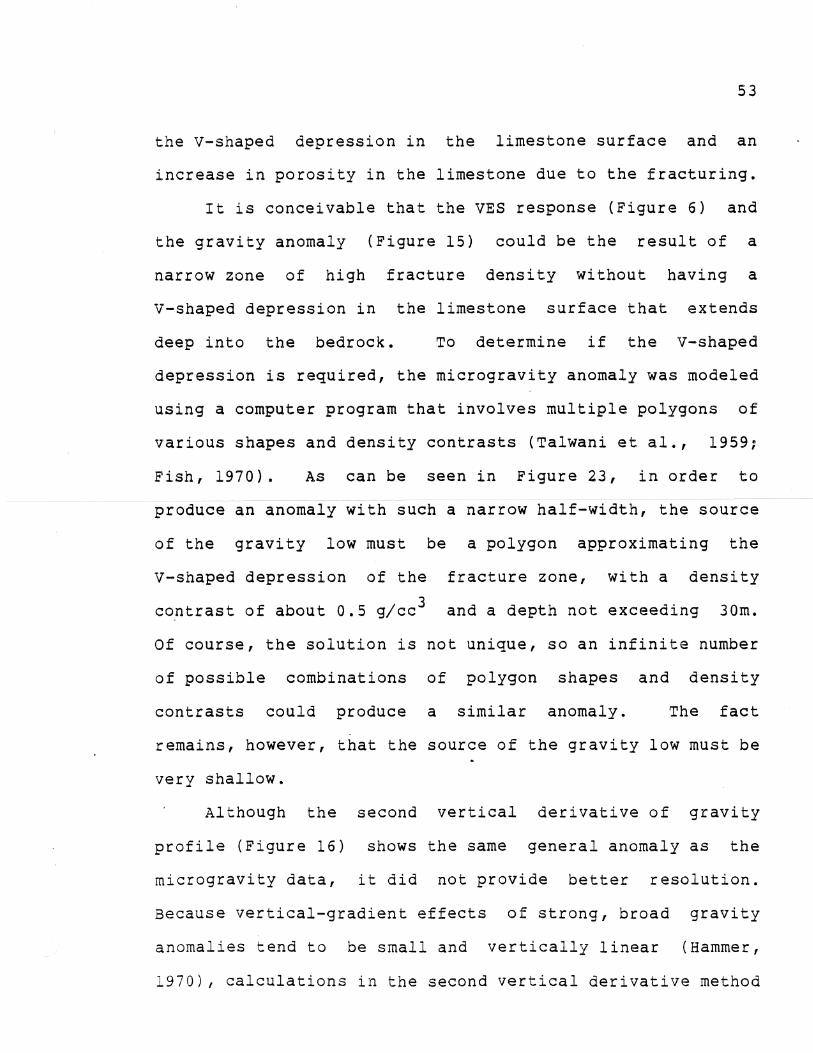
Figure 23. Calculated gravity values and polygons approximating the limestone surface at Cross Bar Ranch.

east

55

enhance instrument and survey inaccuracies as well as real

anomalies. Extreme care must be taken with elevation and

instrument readings and with data reductions to minimize the

possibility of noisy data. The surveys along profiles NF

and SF are too noisy to allow for enhancement of the anomaly

by the second vertical derivative method.

EM profiling, (Figures 19 and 20), measures the terrain

conductivity, which is the inverse of resisitivity, of the

geoelectric section directly. The EM data should, therefore,

correlate with the HEP and tri-potential data. Of the

profiles measured by HEP and tri-potential methods, only

---~ -----~~~~~-p_r-o-f-±-l---e----ss-F---w-±t h a 4-(}m-c-or-1--spa-c±ng~-anu---v e r t i ca-i d i po :te-g-----~~-

shows a major conductivity high at about 20E. The other

profiles in the southern part of the trace show many small

anomalies but none that are obvious or indicative of a

fracture zone.

To the north, profiles NF and NEF both reveal distinct

conductivity highs with both 20m and 40m coil spacings and

vertical dipoles. -The location of the conducti vi ty highs

are consistent with the other data between stations lOE and

SOE, although the peaks vary with the depth of exploration.

This would suggest that the source of the anomaly is

vertically discontinuous (i.e., the

20m coil spacing may be due to the

broad responses of the

thickening of the clay

unit over the V-shaped depression of the limestone surface

while the sharper responses of the 40m coil spacing may be

56

due to clay-filled or water-filled fractures within the

limestone bedrock).

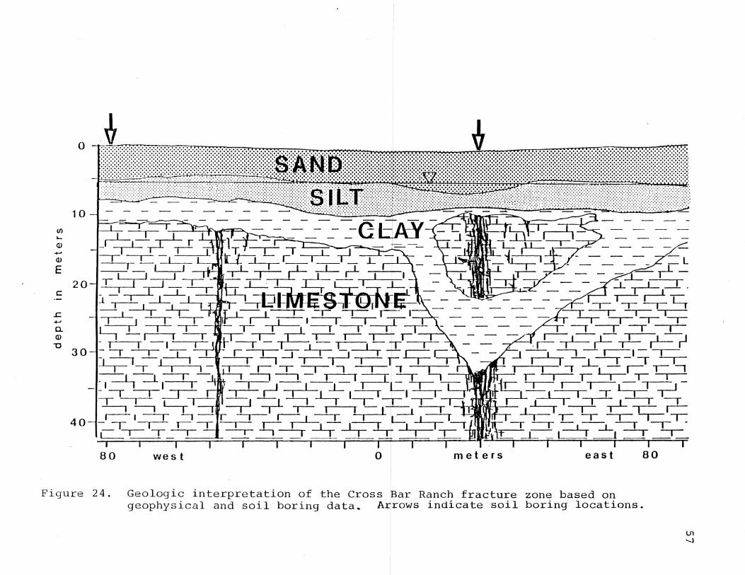
The geometry of the fracture zone at Cross Bar Ranch

and the geologic interpretation is shown in Figure 24. The

geometry is what would be expected for a vertical fracture

in soluble limestone. The thickening of the overlying,

unconsolidated deposits over the trace indicates that the

fracture zone and associated solution features may have been

developing since before deposition of the clay unit, which

is Miocene or younger in age (Moore and Stewart, 1983).

This should provide enough time for development of the

V-shaped depression in the limestone bedrock by weathering

and solution created by aggressive groundwaters moving

downward through the fractures. It should be noted that

exploratory drilling to the first limestone. encountered

would not defipe or delineate the fracture zone.

In correlating the geophysical data, the fracture zone

is located approximately 30m east of the trace center. The

geophysical responses of the fracture zone are fairly linear

over long distances but can vary as much as 40m laterally

within profiles only 100m apart. Also, the fracture zone

appears to made up of several fractures that are vertically

discontinuous and variable in depth. This is probably due

to the karstic nature of the limestone. On a relatively

small scale, solution develops irregularly along bedding

.~

10

(f) .... <1l

...... <1l

E 20

c

..c

...... 0. <1l

"0 30

40

Figure 24. Geologi~ interpret~tion of the Cross ~ar R~nc~ fractu~e zon~ based o~ geophyslcal and sOll boring data. A~rows lndlcate sOlI borlng locatlons.

lJ1 -...J

58

planes and fractures, and confining stresses keep fractures

to a minimum at depth.

Crystal River Quarry No.2

As at Cross Bar Ranch, closely-spaced, vertical

electric soundings provided the most information on the

stratigraphy and the geometry of the fractured limestone at

Crystal River Quarry No.2. A soil boring was completed at

station 50NW to calibrate the VES data because none of the

geophysical data indicated any fracturing of the limestone.

The VES data (Figure 8) correlate well with the soil borin9 __ . __ _

at 50NW (Table 4) in which three distinct lithologies are

present. Surficial sand and sandy clay units with increasing

clay content toward the base, overlie the limestone bedrock

(i.e., the Crystal River Formation of the Ocala Group;

vernon,1951). As discussed previously, the clayey unit

consists of less than 19 percent clay but the entire unit

takes on the physical and electrical characteristics of a

clay. Th~ geometry of the fracture zone is very different

from that at Cross Bar Ranch. From the VES data shown in

Figure 8, instead of a deep V-shaped depression, the

limestone surface exibits a ridge with lO-15m of relief and

a narrow V-shaped depression in the center at station O.

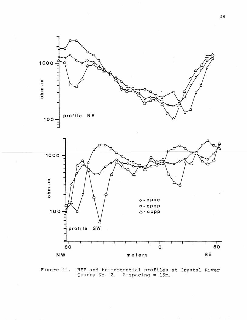
The HEP and tri-potential profiles (Figure 11) show

major divergences of the apparent resistivities of the CPCP

59

and the CCPP arrays on both profiles. These divergences are

not defined by Ogden and Eddy's (1984) classification of

tri-potential responses. Profile NE has divergences near

the trace center at stations 12NW and 12SE. This conflicts

with the YES data, which indicate the fracture center at

station O. To resolve this difference, a soil boring was

selected at station 15SE. As seen in Table 5, the near­

surface stratigraphy correlates well with the YES data. The

YES data indicate the top of limestone at about 10m below

land surface, the soil boring revealed abundant limestone

fragments starting at 9.3m and continuing until the top of

c-omp-e-e-~n-ch'-nre~on-e-wQg-encuun t-e rtITi------arZ-Sm. Pres umably , a

clay-filled fracture exists at about 15SE within the more

resistant ridge. A similar discrepancy between the YES and

the tri-potential da.ta exists at station 72NW. A soil

boring at 72NW did not encounter limestone until 34.5m below

land surface while the YES suggested the top of limestone at

a depth of about 16.5m, which indicates another clay-filled

fracture.

It can be assumed that the other, similar divergences

of the CPCP and CCPP arrays along profiles NE and SW are

also clay-filled fractures. The three distinct divergences

are equally spaced with respect to each profile and

represent linear, clay-filled fractures in the limestone

that are oriented at some strike other than that of the

60

trace. Thus, the fractures tend to wander within the

photolinear over small distances.

The HEP data are only useful along profile NE where

they define a broad resistivity low with a minimum at

station 12SE. All the tri-potential anomalies are marked by

resistivity lows in HEP data, but the magnitude of the HEP

anomalies are not significant enough to make the HEP method

particularly useful by itself.

It is interesting to note that the electrode spacing

(15m) used for the profiling was selected on the basis of

the VES data, which indicate depth to bedrock about 10m near

------------t-he-e-e-n-t-e-r----o-f--t-he-t-r-ae e • Th-i-s-i--s------i • 5 t ±-me-s-t-he---dept-h--tor---­

bedrock as opposed to 1.3 times suggested by Kirk (1976).

To the sides of the trace the depth to bedrock is much

greater (20m or more). The tri-potential method, however,

detected a clay-filled fracture that extended over 40m deep.

This suggests that the effect of the fractured limestone is

expressed well up into the overlying unconsolidated units

and at least some of the fracturing post-dates depostion of

the sandy clay unit.

The azimuthal survey (Figure 14) has the same A-spacing

(15m) as the electrical profiling. Unlike the azimuthal

survey at Cross Bar Ranch, almost all the resistivity

ellipses at Crystal River Quarry No. 2 show a high degree of

anisotropy regardless of location with respect to the

fractures. The ellipse at station 2W has a significant

61

resistivity low that pinches the ellipse in almost the same

azimuth as the strike of the trace and is located over the

trace center according to the VES data. But the ellipse at

station 32E, shows even more anisotropy in a direction

almost 90 0 to the azimuth of the fracture trace. It seems

evident that the azimuthal method is difficult to interpret

for locating buried fractures and provides little

. information on the stratigraphy.

The microgravity profiles (Figure 17) both show an

apparent dip in bedrock surface to the southeast. This

apparent dip is also seen in the VES data. In profile NE, a

----,smalL-9-r-av--iL~1o-w-o-f---abou-t----O-.-l5____11l941 ex i s t-s-cO-th-e s ou thea.~s-\o.t--­

of the trace center, but the survey is too noisy and does

not indicate any major anomalies that correspond with

fractures detected by.the other methods. This suggests that

a large zone of fracture concentration does not exist.

Perhaps, a zone of few fractures which are recystallized or

clay-filled exist near the trace center. The bulk porosity

of the limestone in.the fractured areas is not great enough

to produce significant gravity lows.

As expected from a noisy microgravity survey that does

not exibit any major anomalies, calculations of the second

vertical derivative of gravity (Figure 18) for these

profiles do not enhance the interpretation. The data become

noisier as inaccur~cies in measurement or data reduction are

magnified. The extra time involved in collecting data for

62

the calculations of the second vertical derivitive of

gravity does not appear to be worthwhile in a microgravity

survey where the expected anomalies are so small.

The EM profiles (Figures 21 and 22) seem to correlate

reasonably well with each other. They reveal conductivity

highs at similar stations for both 20m and 40m coil spacings

with vertical dipoles. This indicates that the source of

the conductivity highs (clay-filled fractures) are

vertically continuous. When compared to the HEP and

tri-potential profiles, profile SW shmvs excellent

correlation with a conductivity high at station 40W and it -~ -----

appears to group the fractures at l7SE and 37SE together as

a broad conductivity high. This may be due to the greater

depth of exploration achieved and to measuring the bulk

conductivity of the formation, which could be influenced by

both clay-filled fractures.

Along profile NE, the EM data do not show a close

agreement with the HEP and tri-potential data. The fracture

at station 72NW is barely noticeable on the EM profiles and

a sharp peak observed at 20NW-30NW does not correlate with

any of the electrical-profiling data. The geoelectric cross

section (Figure 9), however, indicates a "pocket" of very

low resistivity between stations 20NW and 30NW which dips

toward the fracture detected at 12NW. This may be a plug of

very clayey material that is not vertically continuous

between station 20NW and 30NW. The tri-potential method is

63

most sensitive to lateral variations in resistivity oriented

in the vertical sense. A conductivity high at about lOSE

correlates well with the fracture at ISSE and another, quite

significant conductivity high is located at about SOSE-60SE.

No HEP or tri-potential measurements were made here for

correlation. The geoelectric cross section (Figure 9) also

shows a -pocket- of low resistivity between stations SOSE

and 60SE. This low possibly represents a very clayey plug

that may be fracture related.

The geometry of the fracture zone and geologic

interpretation at Crystal River Quarry No. 2 are shown in

-----F-i-gu-r-e 25. The geol-ogy-----±s iIlterprete-d-t-o--be a ridg~e"'-----co.....Ff---~

fractured recrystallized limestone. The bedrock surface has

an apparent dip to the ~outheast. A narrow, V-shaped

depression, where solution development has been greatest,

exists in the center of the trace. The presence of clay-

filled fractures within the recrystallized ridges on either

side of the central fracture zone are consistent with those

observed in outcrop -on the quarry walls. The limestone on

either side of the central fracture zone is harder and

recemented when compared to the limestone away from the

fracture zone. This causes the resistivities to be higher,

since the bulk porosity is lower. Again, drilling to the

top of limestone probably would not detect or define the

fracture zones, although for different reasons than at Cross

Bar Ranch.

10

(f) ... Q)

..... Q) 20 E c

.t=

...... Q

30 Q)

"0

40

I ',',~~ ~=-~ " ~I~) ',', I"'~ ':li 1 , 1 L---.J , --L .- I , jj I __ I I 1 1 I I I 1-'-~ I -r-TI I 1_-,.1- IL ~--.J

--r-.L-'=-' I I I T _ -. L . .- I -.- _-.l 1 I 1 --L I -L' I I ,------..L ----L

--'1 r-r --:-L ---. , 1---1.-- J __ ~- , I --I --1- . --2 -:---'4-. -.-t- , I ' -. I -r ~ T -. It i I I i -,-;-r---, I_,-r I I

--..-L- ,-. --.-J -1-- _r-=1 -r -r- _ I I _ ---L-- _ _ r--L--.! _ 1 ..,-- , T I _, -.-1 _, -.--J 1

I -r I I Ii. .

80 NW o me t e r s SE 80

Figure 25. Geologic interpretation of the Crystal River Quarry No.2 fracture zone based on geophysical and soil boring ¢ata: Arrows indicate soil borinq locations.

0'1 ~

65

The various geophysical data correlate well and define

the fracture zone as two, parallel, fracture sets near the

trace center. Not unlike the trace at Cross Bar Ranch, the

fractures tend to wander within the photolinear at some

strike other than that of the trace. Over longer distances,

however, the fracture zone appears to be almost perfectly

linear.

The fracture detected at 72NW is not evident in the YES

data and does not seem to affect the surface of the

limestone, as does the fracture zone near the trace center,

and no apparent evidence is expressed on land surface. - ----

perhaps-this is an isolated, clay-filled fracture that is

not associated with a zone of high fracture density.

66

CONCLUSIONS

The results of this integrated geophysical study

demonstrate that fracture traces in the carbonate bedrock of

west-central Florida can have very distinctive geophysical

responses. The geophysical responses over the fracture

zones were associated with increased depth and thickness of

the geoelectric layers, microgravity lows, resistivity lows

and conductivity highs. These responses are consistent with

previous geophysical investigations ill kars t re-gi-ons--;---Moor-e---­

and Stewart (1983) showed a thickening of the unconsolida·ted

units and a depression of the limestone surface over

fracture traces. Johnson (1966), Kirk (1976) and Ogden and

Eddy (1984) indicate that fractures normally are zones of

resistivity lows due to an infilling of clay, water, or

other less-resistive sediments. Omnes (1975) and Moore and

Stewart (1983) found gravity lows associated with fracture

traces due to loose low-density material, solution

development, and depressions in the limestone surface.

Closely-spaced, vertical electric soundings yield the

. most information on the stratigraphy and geometry of the

fracture zone and aid in the interpretation of the character

of the fractured limestone. Horizontal electric profiling

is sensitive to lateral changes in resistivity and can be

useful in

center of

locating a resistivity low

the fracture zone. The

67

associated with the

tri-potential method

provides additional information that is useful in detecting

isolated fractures that may not be associated with large

fracture zones. Azimuthal resistivity ellipses may show a

high degree of anisotropy with the minor axis (lowest

resistivity) oriented in the same azimuth as the strike of

the trace, but the ellipses are not always reliable and

should not be used alone as a prospecting tool.

A problem facing all the electrical methods is that of

distinguishing between a clay-filled fracture and a water-

filled fracture, because the resistivity of each is very

low. It is necessary then, especially when prospecting for

high yield wells, to correlate the geophysical data with the

stratigraphy of the area by comparison with soil borings or

drillers' logs.

The microgravity profiles were successful in determining

major changes or variations in the bedrock surface which

correlated with the VES sections. Extreme care must be

taken in field methods and data reduction, however, or

detection of very small anomalies will be over-shadowed by

noisy data. Calculation of the second vertical derivative

of gravity using three closely-spaced microgravity profiles

is highly susceptible to instrument and data reduction

inaccuracies and did not prove to be useful in this study.

EM profiling detected major conductivity highs that

68

correlated with the electrical profiles in most situations,

but profiling was not useful in detecting isolated

fractures.

The geologic character of the two fracture traces is

very different. The

V-shaped depression

Cross Bar Ranch feature is a deep,

in the limestone with considerable

relief where dissolution has been the dominant process. The

Crystal River Quarry feature is a linear ridge of moderate

relief with a central depression. Development of this

feature has been more complex because movement of saturated

groundwater through the fractures has created a cemented,

harder, less porous limestone within the trace. This has

resulted in a more resistant ridge subject to differential

weat~ering. The small, V-shaped depression in the limestone

probably represents the major fracture zone, but fractures

are present on the adjacent ridges as well.

Although photolinears often represent fracture zones,

many hydrogeologically-important fractures may exist

are not expressed on aerial photos or the land surface.

is recommended that multiple geophysical methods be

that

It

used

when determining the location of the fracture zone within

the zone defined by a photolinear or when prospecting for

unmapped fractures. In karst terrains, geophysical methods

are particularly useful as karstification often enhances

fracture zones that may only be a few meters wide.

69

LIST OF REFRENCES

Arzi, A.A.,.1975, Microgravity for engineering applications: Geophys. Prosp., v. 23, p. 408-425.

Blanchet. P.H., 1957, Development of fracture analysis as an exploration method: Am. Assoc. Petroleum Geologists Bull., v. 41, p. 1748-1759.

Carpenter, E.W., and Habberjam G.M., 1956, A tri-potential method of resistivity prospecting: Geophysics, v. 21, p. 455-469.

Cherry, R.N., Stewart, J.W., and Mann, J.A., 1970, General hydrology of the Middle Gulf area, Florida: Florida Bureau of Geology, R.I. 56, Tallahassee, Florida, 96 p.

Fajklewicz, Z.J., 1976, Gravity vertical gradient measurements for the detection of small geologic and anthropogenic forms: Geophysics v.4l, p. 1016-1030.

Fenneman, N.H., 1928, Physiographic divisions of the United States: Am. Assoc. Geographers Bull., v. 18, p. 17-24.

Fish, J.E., 1971, Crustal structure of the Texas Gulf coastal plain: M.A. thesis, Dept. of Geology, University of Texas at Austin, Austin, Texas, 29 p.

Florquist, B.A., 1973, Techniques in fractured rocks: Ground 26-28.

for locating water Water, v. 11, no.

wells 3, p.

Gilboy, T., and Moore, D., 1982, Hydrologic analysis Cross Bar Ranch Wellfield: Southwest Florida Water Management District, Brooksville, Florida, 37 p.

Habberjam, G.M., 1969, The location of spherical cavities using a tri-potential resistivity technique: Geophysics, v. 34, no. 5, p. 780-784.

Hammer, S., gravity:

1970, The anomalous vertical gradient Geophysics, v. 35, no. 1, p. 153-157.

of

70

Johnson, P.W., 1966, Investigation of photogeologic fracture traces by electrical prospecting methods: M.S. thesis, Dept. of Geology and Geophysics, pennsylvania State University, University Park, pennsylvania, 94 p.

Kirk, K.G., 1976, Tri-potential resistivity technique in locating cavities, fracture zones, and aquifers: M.S. thesis, Dept. of Geology, West Virginia University, Morgantown, West virginia, 105 p.

LaRicca, M.P., and Rauch H.W., 1977, Water well productivity related to photo lineaments in carbonates of Fredrick Valley, Maryland: Hydrologic Problems in Karst Regions, Western Kentucky University, Kentucky, p. 228-234.

Lattman,L.H., and Parizek, R.R., 1964, Relationship between fracture traces and the occurrence of groundwater in carbonate rocks: Jour. of Hydrology, v. 2, p.73-91.

LeGrand, H., 1979, Evaluation techniques of fractured-rock hydrology: Jour. of Hydrology, v. 34, p. 333-346.

- -- - -

Leonard-Mayer, P.J., 1984, Development and use of azimuthal resistivity surveys for jointed formations: Surface and Borehole Geophysical Methods in Ground water Investigations, NWWA Symposium Proceedings, San Antonio, Texas.

McNeill, J.D., 1980, Electromagnetic terrain conductivity measurements at low induction numbers: Technical Note, 6, Geonics Ltd., Mississauga, Canada, 15 p.

Menke, C.G., Meredith, E.W., and Wetterhall, W.S., 1961, Water resources of Hillsborough County, Florida, 91 p.

Miller, J.C., 1977, Fracture trace analysis for well siting in carbo~ate karst terrain, Crossbar Ranch Wellfield, Pasco County: West Coast Regional Water Supply Authority, Clearwater, Florida, 11 p.

Moore, D.L. and Stewart, M.T., 1983, Geophysical signatures of fracture traces in a karst aquifer (Florida, U.S.A.): Jour. of Hydrology, v.61, p. 325-340.

Nettleton, L.L., 1940, Geophysical Prospecting for Oil: McGraw-Hill, New York, New York, 411 p.

Omnes, G., 1975, Microgravity and its application to engineering: Transportation Research Board Record 54th Annual Meeting, Washington, D.C., p. 42-51.

civil 581.

71

Ogden, A.E. and Eddy, P.S., 1984, The use of tri-potential resistivity to locate fractures, faults, and caves for siting high-yield water wells: Surface and Borehole Geophysical Methods in Ground water Investigations, NWWA Symposium, San Antonio, Texas.

Parasnis, D.S., 1966, Mining geophysics: Elsevier publ., Amsterdam, 356 p.

Parizek, R.R., 1976, On the significance of fracture traces and lineaments in carbonate and other terrains: in, Karst Hydrology and Water Resources, proceedings US-Yugoslav Symposium, Dubrovnik, water Resources publications, v. 1, p. 47-108.

Setzer, J., 1966, Hydrologic significance of tectonic fractures detectable on air ph6tos: Ground Water, v. 4, p. 23-27.

Siddiqui, S.H., and Parazek, L.L., 1971, Hydrologic factors influencing well yields in folded and faulted carbonate rocks in central Pennsylvania: Water Resources Research, v. 7, No.5, p. 1295-1312.

Smith, D.L., and Randazzo, A.F., 1975, Detection of subsurface solution cavities in Florida using electrical resistivity measurements: Southeastern Geology, v. 16, no. 4, p. 227-240.

Streltsova, T.D., 1976, Hydrodynamics of ground water flow in a fractured formation: water Resources Research, v. 12, no. 3, p. 405-413.

Talwani, M., Worzel, J.L., and Landisman, M., 1959, Rapid gravity computations for two-dimensional bodies with applicatIon to the Mendocino submarine fracture zones: Jour. Geophy. Research, v. 64, p. 49-59.

Taylor, R.W., 1984, The determination of jointed orientation and porosity from azimuthal resistivity measurements: Surface and Borehole Geophysical Methods in Ground Water Investigations, NWWA Symposium proceedings, San Antonio, Texas.

Telford, W.M., Geldart, L.P., Sheriff, R.E., and Keys, D.A., 1976, Applied Geophysics: Cambridge University Press, New York, New York, 860 p.

72

Thyssen-Bornemisza, 5., 1965, von Horizontalgradienten Schwereprofilen: zeitschr. p. 58-60.

Die gleichzeitige Bestimmung und wzzz aus drie engen Geophys~k (Germany), v. 32,

vernon, R.O., 1951, Geology of Citrus and Levy Counties, Florida: Florida Bureau of Geology, Bull. 53, Tallahassee, Florida, 255 p.

wobber, F.J, 1967, Fracture traces in Illinois: metric Engineering, v. 33, p. 499-506.

zohdy, A.A.R, and Bisdorf, R.J., 1975, An inversion of Wenner sounding curves by convolution: National Technical Information Springfield, virginia, Publ. 247-265, 28 p.

Photogram-

automatic MDZ and Service,

73

-----------------------------------------

APPENDIXES

74

APPENDIX I

VERTICAL ELECTRIC SOUNDING DATA

1. Apparent resistivities are in ohm-meters

2. BOW: Vertical Electric Sounding at Station BOW

3. A-sp~cing is AB/3 distance in meters for Wenner Array

4. *: Missing data

75

Table 7. Vertical electric sounding data at Cross Bar Ranch.

A-spacing 80W 40W 0 10E 20E 30E 40E 50E 85E

1 1605 1796 1672- 1188 1559 1595 1865 1473 1716 2 2324 2411 3281 1999 2394 2063 2645 2315 2851 3 2474 2575 2389 2117 2533 2214 2942 2742 3563 4 2140 2223 2111 1602 2500 2257 2896 3041 3465 6 1741 1654 1876 1238 2218 1737 1979 2554 3440

10 827 628 785 741 1104 1010 1010 1487 2076 15 320 238 417 299 375 422 427 613 1107 20 181 166 186 177 239 288 254 348 492 30 130 141 132 152 * 190 181 213 197 40 130 137 146 142 149 156 154 167 153 50 141 136 145 150 157 146 149 149 155 60 139 132 143 151 170 153 154 156 154 80 * * 161 * * 163 * * *

100 * 168 * * * * * * *

76

Table 8. Vertical electric sounding data at Crystal River Quarry No.2.

A-spacing 95NW 80NW 70NW 55NW 30NW 20NW 10NW 0 lOSE 20SE

1 5511 6412 4448 5575 4797 4216 1140 1093 6001 4498 2 7046 7928 6315 7138 5856 4850 1230 1642 4609 3948 3 5313 7599 7037 6670 5023 3676 971 1288 2723 2582 4 4455 6852 7816 5982 3715 3152 829 903 1584 1979 6 2809 5938 4834 4353 1806 1276 707 681 1033 1231

10 1018 1961 1961 1637 721 523 359 470 595 743 15 408 575 662 517 409 * 133 * * * 20 265 203 230 212 208 172 107 135 166 198 30 121 114 121 129 163 113 120 129 107 91 50 126 ·130 115 126 154 130 134 126 126 129 70 132 170 147 127 156 169 154 132 161 132

--A spacing 3ilSE----s-frS-E-i:iTfrSE

1 2840 8990 6120 2 2477 5352 5656 3 1501 4807 5550 4 949 3958 4908 6 576 3063 4989

10 546 2386 5320 15 * 1907 * 20 326 944 3709 30 102 232 1979 50 120 137 1009 70 132 141 453

100 * * 174 160 * * 110

77

APPENDIX II

HORIZONTAL ELECTRIC PROFILE AND TRI-POTENTIAL DATA

1. Apparent resistivities in ohm-meters.

2. lOOW: station at center of array at which reading was taken.

3. A-spacing is AB/3 distance in meters.

4. CPPC: Wenner array (HEP)

5. CPCP: Bipole-bipole array

6. CCPP: Dipole-dipole array

78

Table 9. Horizontal electric profile and tri-potential data at Cross Bar Ranch.

A = 50 meters A = 50 meters

Profile SSF CPPC CCPP CPCP Profile SF CPPC CCPP CPCP

100W 140 173 126 100W 126 157 165 90W 142 158 138 90W 123 141 146 80W 161 132 143 80W 143 165 152 70W 165 132 169 70W 141 157 168 60W 157 138 156 60W 144 188 168 SOW 151 157 176 50W 136 188 184 40W 145 169 149 40W 145 177 183 30W 136 156 136 30W 144 168 173 20W 136 151 143 20W 144 179 178 lOW 151 168 179 lOW 151 165 165

0 163 151 180 0 140 151 161 l-OE 157 151 172 10E 1-3-9----1-6 5 1'73 20E 138 151 168 20E 117 165 184 30E 140 209 151 30E 141 235 154 40E 126 194 123 40E 136 172 151 50E 142 175 129 50E 134 170 151 60E 130 176 141 60E 136 189 141 70E 138 151 163 70E 139 172 151 80E 142 158 179 80E 141 165 161 90E 126 151 182 90E 147 170 165

100E 146 137 168 100E 136 165 165

79

Table 9 (continued).

A = 50 meters

Profile NSF CPPC CCPP CPCP

100W 149 189 161 90W 147 189 163 80W 145 165 165 70W 141 170 151 60W 144 141 150 SOW 152 170 160 40W 129 172 154 30W 141 189 157 20W 150 151 165 lOW 136 165 154 00 157 138 160 10E 141 141 173 20E 149 J.e-f 177 30E 155 189 154 40E 144 172 150 50E 141 165 172 60E 149 165 160 70E 122 235 151 80E 173 199 165 90E 157 -172 168

100E 141 179 157

80

Table 10. Horizontal electric profile and tri-potential data at Crystal River Quarry No.2.

A = 15 meters A = 15 meters

Profile NE CPPC CCPP CPCP Profile SW CPPC CCPP CPCP

87NW 1330 1816 1113 82NW 99 94 131 82NW 1285 1882 1001 77NW 303 134 410 77NW 1441 2511 406 72NW 477 99 684 72NW 1126 2573 396 67NW 673 202 833 67NW 1017 2064 530 62NW 584 746 575 62NW 1132 1610 915 57NW 468 1271 180 57NW 1072 1464 966 52NW 471 1564 66 52NW 915 1138 851 47NW 628 1525 203 47NW 741 767 737 42NW 726 1343 456 42NW 647 613 696 37NW 833 1120 772 37NW 546 578 518 32NW 734 990 631 32NW 353 493···· 355 . 27NW 707 -825 594 27NW 345 399 333 22NW 648 776 467 22NW 335 365 337 17NW 641 646 689 17NW 301 349 286 12NW 632 580 585 12NW 232 337 207 7NW 813 660 923

7NW 247 323 218 2NW 735 707 762 2NW 247 289 232 2SE 796 738 867 2SE 212 250 199 7SE 749 1225 471 7SE 184 288 133 12SE 707 1346 336

12SE 174 319 107 17SE 704 1508 299 17SE 196 210 193 22SE 895 1343 801 22SE 257 136 344 27SE 1115 1106 746 27SE 408 153 545 32SE 1058 1074 1123 32SE 572 302 771 37SE 943 1588 801 37SE 794 422 993 42SE 886 1887 613 42SE 1176 747 1431 47SE 1077 1541 887 47SE 1393 1321 1488 52SE 1508 1414 1706 52SE 1775 1901 1771 57SE 2694 1463 2460 57SE 1903 2870 1384 62SE 2662 1696 3589 62SE 2225 3194 1739 67SE 3376 2474 4382

APPENDIX III

AZIMUTHAL RESISTIVITY DATA

1. Apparent resistivities are in ohm-meters.

2. 60W: Station at center of array.

3. A-spacing is AB/3 distance in meters.

81

82

Table 11. Azimuthal resistivity data.

Cross Bar Ranch: A = 30 meters

STATION 650 95 0 1250 1550 1850 2150

60W 132 132 135 138 129 140 40W 135 140 142 134 143 157 20W 127 132 140 140 134 138

0 148 113 165 140 136 140 20E 153 151 163 187 144 143 30E 167 138 172 167 173 143 40E 172 134 136 191 181 161 50E 180 158 136 184 183 180 60E 179 172 156 152 199 174

100E 192 178 161 158 206 163

Cross Bar Ranch: A = 75 meters

STATION 65 0 95 0 1250 1550 1850 2150

15W 165 165 153 153 153 161 5W 173 150 153 153 153 153 5E 165 165 153 163 168 161

10E 161 153 165 157 153 169 20E 165 157 165 153 161 165 25E 153 157 167 165 161 167 45E 141 153 173 161 165 161

Crystal River Quarry No.2: A = 15 meters

STATION 1'350 1650 1950 2250 2550 2850

72NW 559 564 485 603 489 476 52NW 472 457 374 315 348 357 42NW 456 487 324 309 277 361 32NW 380 385 337 372 309 396 22NW 289 199 274 277 229 292 12NW 220 241 158 170 203 283

2NW 236 280 281 157 224 238 12SE 174 249 380 401 388 228 22SE 265 517 523 328 197 144 32SE 599 1309 1035 734 452 158 60SE 2004 1428 1000 1288 2256 2584

lOOSE 7573 8137 7823 8256 8001 6987

APPENDIX IV

GRAVITY DATA

1. Elevations corrected to zero datum along indivi~ual profiles.

83

2. Bouguer gravity (mgals) = (observed instrument) + (drift correction) + (latitude correction) + (elevation correction) + (Bouguer correction).

3. Bouguer gravity is relative gravity along individual I profiles.

4. Vertical gradient of gravity (gl) was calculated from three closely-spaced profiles:

at station c 2 :

gl = I/s2*(4C2-(a2+c3+b2+cl»

Where: s = station spacing and,

--a --a --a --a --I 234

--cl --c2--c3--c4--

--bl --b2--b3--b4--

84

Table 12. Gravity data at Cross Bar Ranch.

PROFILE SF

Station Bouguer Station Bouguer Station Bouguer

SlOOW 184.66 100W 184.66 NI00W 184.67 S95W 184.61 95W 184.65 N95W 184.70 S90W 184.66 90W 184.63 N90W 184.68 S85W 184.65 85W 184.63 N85W 184.69 S80W 184.69 80W 184.65 N80W 184.65 S75W 184.68 75W 184.67 N75W 184.61 S70W 184.69 70W 184.62 N70W 184.65 S65W 184.70 65W 184.61 .N65W 184.70 S60W 184.69 60W 184.62 N60W 184.70 S55W 184.72 55W 184.63 N55W 184.68 S50W 184.69 50W 184.63 N50W 184.71 S45W 184.69 45W 184.63 N45W 184.60 S40W 184.75- 40W 184.71 N40W 184.74 S35W 184.72 35W 184.70 N35W 184.77 S30W 184.72 30W 184.67 N30W 184.74 S25W 184.74 25W 184.67 N25W 184.74 S20W 184.72 20W 184.68 N20W 184.76 S15W 184.69 15W 184.71 N15W 184.77 SlOW 184.65 lOW 184.71 NI0W 184.75

S5W 184.62 5W 184.68 N5W 184.67 SO 184.65 0 184.67 NO 184.71 S5E 184.63 5E 184.63 N5E 184.70

SlOE 184.64 10E 184.62 NI0E 184.73 S15E 184.66 15E 184.63 N15E 184.69 S20E 184.48 20E 184.58 N20E 184.67 S25E 184.50 25E 184.59 N25E 184.64 S30E 184.65 30E 184.62 N30E 184.67 S35E 184.59 35E 184.60 N35E 184.66 S40E 184.64 40E 184.56 N40E 184.60 S45E 184.65 45E 184.58 N45E 184.64 S50E 184.63 50E 184.57 N50E 184.71 S55E 184.65 55E 184.63 N55E 184.74 S60E 184.63 60E 184.63 N60E 184.66 S65E 184.64 65E 184.68 N65E 184.74 S70E 184.64 70E 184.69 N70E 184.70 S75E 184.70 75E 184.71 N75E 184.79 S80E 184.68 80E 184.72 N80E 184.76 S85E 184.71 85E 184.70 N85E 184.77 S90E 184.69 90E 184.68 N90E 184.78 S95E 184.66 95E 184.67 N95E 184.76

S100E 184.70 100E 184.74 NI00E 184.75

85

Table 12 (continued).

PROFILE NF

Station Bouguer Station Bouguer Station Bouguer

S40W 190~80 40W 190.71 N40W 190.76 S35W 190.73 35W 190.73 N35W 190.72 S30W 190.79 30W 190.74 N30W 190.70 S25W 190.72 25W 190.76 N25W 190.70 S20W 190.76 20W 190.78 N20W 190.72 S15W 190.76 15W 190.82 N15W 190.72 SlOW 190.69 lOW 190.76 N10W 190.68

S5W 190.73 5W 190.77 N5W 190.68 SO 190.70 0 190.77 NO 190.72 S5E 190.70 5E 190.77 N5E 190.71

SlOE 190.65 10E 190.77 N10E 190.71 S15E 190.69 15E 190.69 N15E 190.66 S20E 190.67 20E 190.71 N20E 190.65 S25E 190.68 25E 190.71 N25E 190.67 S30E 190.68 30E 190.66 N30E 190.63 S35E 190.74 35E 190.62 N35E 190.72 S40E 190.68 40E 190.65 N40E 190.70 S45E 190.68 45E 190.71 N45E 190.69 S50E 190.71 50E 190.68 N50E 190.69 S55E 190.73 55E 190.75 N55E 190.67 S60E 190.67 60E 190.68 N60E 190.67 S65E 190.70 65E 190.74 N65E 190.69 S70E 190.73 70E 190.77 N70E 190.72 S75E 190.73 75E 190.82 N75E 190.72

. S80E 190.72 80E 190.75 N80E 190.73 S85E 190.72 85E 190.81 N85E 190.73 S90E 190.72 90E 190.78 N90E 190.72 S95E 19'0.69 95E 190.78 N95E 190.79

S100E 190.69 100E 190.77 N100E 190.69 S105E 190.70 105E 190.78 N105E 190.73 Sl10E 190.68 110E 190.79 N110E 190.71 Sl15E 190.70 115E 190.75 Nl15E 190.70 S120E 190.64 120E 190.72 N120E 190.71 S125E 190.67 125E 190.70 N125E 190.61 S130E 190.67 130E 190.70 N130E 190.66 S135E 190.66 135E 190.61 N135E 190.65 S140E 190.67 140E 190.52 N140E 190.58

86

Table 13. Gravity data at Crystal River Quarry No.2.

PROFILE SW

Station Bouguer Station Bouguer Station Bouguer

S100NW 177.86 100NW 177.93 NI00NW 177.87 S95NW 177.86 95NW 177.92 N90NW 177.81 S90NW 177.89 90NW 177.91 N90NW 177.86 S85NW 177.90 85NW 177.90 N85NW 177.89 S80NW 177.92 80NW 177.93 N80NW 177.93 S75NW 177.89 75NW 177.91 N75NW 177.90 S70NW 177.87 70NW 177.92 N70NW 177.92 S65NW 177.85 65NW 177.89 N65NW 177.88 S60NW 177.89 60NW 177.93 N60NW 177.87 S55NW 177.86 55NW 177.94 N55NW 177.90 S50NW 177.87 50NW 177.96 N50NW 177.92 S45NW 177.92 45NW 177.98 N45NW 177.92 S40NW 177.89 40NW 177.97 N40NW 177.92 S3-5NW 177.91 35NW 177.95 N35NW I 77--;rr3 S30NW 177.88 30NW 177.96 N30NW 177.91 S25NW 177.90 25NW 177.96 N25NW 177.90 ;"

S20NW 177.91 20NW 177.93 N20NW 177.87 S15NW 177.93 15NW 177.93 N15NW 177.93 S10NW 177.95 10NW 177.95 NI0NW 177.94

S5NW 177.92 5NW 177.94 N5NW 177.92 SO 177.98 0 177.91 NO 177.95 S5SE 177.92 SSE 177.96 N5SE 177.93

S10SE 177.92 lOSE 177.99 NI0SE 177.88 S15SE 177.99 15SE 177.99 N15SE 177.92 S20SE 177.89 20SE 177.93 N20SE 177.92 S25SE 177.91 25SE 177.99 N25SE 177.93 S30SE 177.91 30SE 177.93 N30SE 177.92 S35SE 17'7 .93 35SE 177.88 N35SE 177.94 S40SE 177.89 40SE 177.97 N40SE 177.89 S45SE 177.89 45SE 177.90 N45SE 177.87 S50SE 177.93 50SE 177.90 N50SE 177.89 S55SE 177.90 55SE 177.86 N55SE 177.87 S60SE 177.91 60SE 177.91 N60SE 177.89 S65SE 177.85 65SE 177.84 N65SE 177.91 S70SE 177.86 70SE 177.81 N70SE 177.87 S75SE. 177.90 75SE 177.86 N75SE 177.83 S80SE 177.88 80SE 177.76 N80SE 177.81 S85SE 177.86 85SE 177.78 N85SE 177.76 S90SE 177.83 90SE 177.76 N90SE 177.78 S95SE 177.82 95SE 177.69 N95SE 177.77

S100SE 177.81 lOOSE 177.68 NI00SE 177.79

87

Table 13 (continued).

PROFILE NE

Station Bouguer Station Bouguer Station Bouguer

S100NW 176.66 100NW 176.70 N100NW 176.61 S95NW 176.68 95NW 176.66 N95NW 176.61 S90NW 176.72 90NW 176.6-8 N90NW 176.73 S85NW 176.69 85NW 176.67 N85NW 176.71 S80NW 176.67 80NW 176.66 N80NW 176.62 S75NW 176.68 75NW 176.68 N75NW 176.63 S70NW 176.69 70NW 176.65 N70NW 176.59 S65NW 176.67 65NW 176.66 N65NW 176.61 S60NW 176.66 60NW 176.71 N60NW 176.62 S55NW 176.66 55NW 176.67 N55NW 176.63 S50NW 176.67 50NW 176.67 N50NW 176.63 S45NW 176.63 45NW 176.64 N45NW 176.61 S40NW 176.67 40NW 176.72 N40NW 176.64 S3"SNW 1 T0:07 35NW 176.72 N35NW 176.65 S30NW 176.64 30NW 176.71 N30NW 176.64 S25NW 176.75 25NW 176.70 N25NW 176.68 S20NW 176.70 20NW 176.72 N20NW 176.64 S15NW 176.71 15NW 176.68 N15NW 176.60 S10NW 176.67 10NW 176.73 N10NW 176.69

S5NW 176.67 5NW 176.67 N5NW 176.61 SO 176.56 0 176.64 NO 176.61 S5SE 176.64 5SE 176.66 N5SE 176.60

S10SE 176.67 lOSE 176.65 N10SE 176.60 S15SE 176.54 15SE 176.61 N15SE 176.58 S20SE 176.60 20SE 176.64 N20SE 176.60 S25SE 176.62 25SE 176.56 N25SE 176.60 S30SE 176.66 30SE 176.59 N30SE 176.58 S35SE 11'6.66 35SE 176.59 N35SE 176.61 S40SE 176.63 40SE 176.62 N40SE 176.61 S45SE 176.68 45SE 176.60 N45SE 176.60 S50SE 176.58 50SE 176.62 N50SE 176.59 S55SE 176.59 55SE 176.58 N55SE 176.55 S60SE 176.63 60SE 176.66 N60SE 176.58 S65SE 176.67 65SE 176.67 N65SE 176.59 S70SE. 176.55 70SE 176.61 N70SE 176.58 S75SE 176.56 75SE 176.46 N75SE 176.50 S80SE 176.47 80SE 176.48 N80SE 176.45 S85SE 176.52 85SE 176.41 N85SE 176.54 S90SE 176.43 90SE 176.50 N90SE 176.47 S95SE 176.49 95SE 176.45 N95SE 176.48

S100SE 176.44 lOOSE 176.45 N100SE 176.47

88

APPENDIX V

ELECTROMAGNETIC DATA

1. Apparent conductivities in mmhos/m.

2. 10V: 10 meter coil spacing; vertical dipole.

3. 10H: 10 meter coil spacing; horizontal dipole.

4. 20V: 20 meter coil spacing; vertical dipole.

5. 20H: 20 meter coil spacing; horizontal dipole.

6. 40V: 40 meter coil spacing; vertical dipole.

7 • 40H: 40 meter coil spacing; horizontal dipole.

s. * : Missing data.

89

Table 14. Electromagnetic data at Cross Bar Ranch.

PROFILE SSF PROFILE SF

STATION 20V 20B 40V 40B 20V 20B 40V 40B

100W 7.8 6.2 5.6 5.4 7.5 5.2 5.4 5.2 90W 7.6 6.0 5.6 5.6 7.5 6.0 4.8 5.0 80W 7.4 5.8 5.4 5.6 7.0 5.6 4.9 5.8 70W 7.2 5.6 5.2 5.6 6.4 6.6 5.2 4.8 60W 7.0 5.8 4.8 5.4 8.0 6.2 5.0 5.8 50W 6.6 5.8 4.4 5.4 6.4 6.2 5.4 5.0 40W 6.4 6.4 4.2 5.2 7.2 6.0 5.7 6.2 30W 6.8 6.0 3.8 4.8 6.9 6.2 4.8 5.2 20W 7.2 5.8 4.6 5.0 7.4 6.2 5.4 4.6 lOW 7.4 5.4 6.4 5.0 8.4 6.2 5.2 5.8

0 7.6 5.4 6.2 4.8 7.6 5.8 5.2 5.8 10E 7.8 5.4 6.6 4.8 8.4 5.6 5.0 5.8 20E 8.2 5.6 7.2 6.2 7.6 5.8 5.0 5.6 30E- -7 . 8 - . 6.-0 6.4 5.5 7 . 0- - 5.8 5.2 5.4 40E 8.0 6.2 5.0 5.2 7.2 5.8 5.6 5.2 50E 8.4 6.6 4.0 4.8 7.6 6.2 5.0 5.2 60E 7.8 6.8 4.8 5.0 8.0 5 .. 8 5.0 5.2 70E 8.6 6.8 5.4 5.0 7.6 5.8 4.2 4 •. 8 80E 9.0 7.0 4.8 5.2 7.2 5.8 5.6 5.2 90E 8.6 6.8 5 .. 2 5.5 8.2 5.8 5.6 4.6

100E 7.8 6.6 5.0 5.2 7.6 5.8 6. 0 4.8

90

Table 14 (continued).

PROFILE NSF PROFILE NF

STATION 20V 20H 40V 40H 20V 20H 40V 40H

100W 7.4 5.2 5.6 5.0 * * * * 90W 7.5 5.4 5.8 4.8 * * * * 80W 7.4 5.4 6.2 4.8 * * * * 70W 7.5 5.6 6.2 5.0 * * * * 60W 7.4 5.8 6 .• 2 4.8 9.4 7.5 6.8 6.6 SOW 7.2 6.4 5.8 4.8 9.2 7.4 7.2 6.8 40W 8.2 6.4 5.6 4.8 9.2 7.4 6.8 6.8 30W 8.8 6.2 5.8 5.4 9.0 7.6 6.6 7.0 20W 8.4 6.2 6.0 6.0 8.8 7.6 6.6 5.6 lOW 8.0 6.4 6.4 5.8 8.2 7.4 5.2 7.2

0 7.4 7.0 5.6 6.5 7.4 7.8 4.8 7.0 10E 7.6 6.2 6.4 5.4 8.5 8.0 5.8 7.0 20E 7.6 6.0 6.4 5.8 9.0 8.2 9.0 7.0 :)(JE 7.6 6.0 6~8~~ 10.5 6.0 7.2 7.2 40E 7.4 6.0 7.2 5.4 12.4 7.4 6.5 7.2 50E 7.7 6.2 6.0 5.8 13.5 7.4 6.6 7.2 60E 8.2 6.4 7.2 6.0 9.6 8.0 6.0 6.8 70E 8.4 7.0 6.4 6.2 9.4 8.4 5.8 7.4 80E 7.2 7.0 6.6 6.4 9.0 8.5 5.6 7.4 90E 7.0 7.2 6.8 6.4 9.2 8.6 5.4 7.6

100E 6.8 6.8 7.4 6.4 9.-5 8.8 5.2 7.4 110E * * * * 9.6 9.2 5.0 7.0 120E * * * * 9.8 9.5 4.4 7.6 130E * * * * 9.6 9.0 3.6 8.2 140E * * * * 9.8 8.6 3.8 7.8

91

Table 14 (continued) .

PROFILE NEF

STATION 20V 20H 40V 40H

100W 8.2 6.2 5.2 4.6 90W 8.2 6.2 5.2 4.6 80W 8.4 6.0 5.2 4.8 70W 8.4 6.0 5.8 5.0 60W 8.2 6.2 6.8 5.0 50W 7.8 6.0 6.8 5.2 40W 8.2 6.2 6.6 5.2 30W 8.8 6.2 7.2 5.4 20W 9.0 6.4 7.6 5.4 lOW 9.2 6.6 7.2 4.8

0 9.8 6.2 6.6 5.2 10E 10.6 5.2 7.6 5.2 20E 8.4 6.2 9.2 5.2 30E 7.8 6.4 7.2 5.2 40E 8.0 6.2 7.2 5.2 50E 8.2 6.4 7.4 5.4 60E 8.4 6.6 7.8 5.4 70E 8.8 6.4 7.4 5.6 80E 9.0 6.6 7.2 5.8 90E 9.2 6.2 7.0 5.4

lOOE 8.8 6.2 6.8 5.6

92

Table 15. Electromagnetic data at Crystal River Quarry No.2.

PROFILE SW PROFILE MP

STATION 10H 10V 20V 20H 40V 10H 10V 20V 20H 40V

100NW 9.8 8.6 12.5 6.2 4.0 5.4 8.2 6.8 8.8 8.0 90NW 10.6 8.6 13.2 7.0 2.5 5.0 7.8 6.8 8.4 7.4 80NW 10.8 7.8 11.5 5.0 3.4 5.4 7.2 6.0 8.2 7.8 70NW 7.8 9.5 8.6 6.0 2.8 5.0 7.6 6.4 8.0 7.6 60NW 6.2 9.5 8.2 8.8 4.8 5.6 7.6 6.0 8.0 8.6 50NW 5.2 7.8 6.2 9.2 9.2 4.8 6.6 5.8 8.6 8.6 40NW 5.2 7.4 5.6 9.2 10.5 5.2 6.6 6.2 8.8 8.8 30NW 4.8 7.2 6.4 8.6 8.8 5.6 7.0 5.8 8.8 11.0 20NW 5.2 7.2 5.8 6.4 6.5 5.6 7.2 6.4 8.6 7.8 10NW 5.0 6.2 5.2 7.4 6.5 6.0 8.4 6.8 9.4 7.0

0 4.5 7.8 5.6 8.0 8.5 6.0 9.4 6.6 10.2 8.6 lOSE 3.6 7.2 4.6 9.2 9.5 6.8 9.0 7.6 8.6 8.6 20SE -4.4 5:8 5.4 9.2 9:5 7.5 8.0 8.0 - 7.2 6~6 30SE 4.0 7.2 4.4 8.8 8.0 6.5 8.8 8.2 8.8 5.0 40SE 3.8 6.4 4.2 7.4 6.0 6.8 10.0 8.2 10.8 5.0 50SE 4.2 5.8 4.4 5.5 3.2 7.4 10.5 9.2 9.4 7.2 60SE 3.6 5.2 3.5 4.8 2.8 9.8 11.2 10.0 4.6 6.6 70SE 3.6 4.0 3.4 4.4 3.0 10.2 8.8 9.6 3.0 2.4 80SE 3.2 3.6 3.2 4.2 4.4 6.8 7.4 6.8 3.0 1.5 90SE 2.6 3.2 3.2 3.5 -4.8 4.2 4.5 4.6 3.5 2.6

lOOSE 3.6 2.2 2.8 3.2 4.0 3.2 3.5 2.6 3.6 3.8

93

Table 15 (continued) .

PROFILE NE

STATION 10H 10V 20V 20H 40V

100NW 5.4 8.2 5.8 8.6 9.2 90NW 5.6 10.0 6.0 9.2 9.0 80NW 6.2 9.0 5.6 9.4 8.8 70NW 6.6 6.8 6.0 8.4 8.8 60NW 6.2 7.0 6.2 9.8 8.4 50NW 6.2 7.2 6.4 9.8 7.8 40NW 6.0 7.8 5.6 9.2 11.2 30NW 6.2 9.6 6.0 11.5 13.5 20NW 6.4 10.5 3.8 13.2 9.2 10NW 7.2 10.0 6.0 8.8 7.5

0 8.2 9.5 8.0 11.0 6.4 lOSE 10.0 12.0 10.4 12.0 7.6 20SE 9.2 10.5 10.2 9.0 5.0 30SE 10.0 9.0 9.2 5.2 3.4 40SE 6.6 9.6 7.0 9.4 5.2 50SE 5.8 9.0 5.2 10.2 9.5 60SE 5.8 7.4 3.6 9.0 10.2 70SE 4.0 6.2 3.5 6.8 7.4 80SE 3.4 4.4 3.0 5.8 7.4 90SE 3.2 4.8 2.8 5.0 6.2

lOOSE 2.8 3.8 2.4 4.6 6.2