THE GIBBS-EINSTEIN TENSOR ANALYSIS · the gibbs-einstein tensor analysis with application to...

RR 221

mResearch Report 221

THE GIBBS-EINSTEIN TENSOR ANALYSISWITH APPLICATION TO

CONTINUUM MECHANICS AND' CANONICAL FORMS OF

GENERAL SECOND-ORDER TENSORSShunsuke Takagi

November 1968

DDC

AN 2 3,19

C

U.S. ARMY MATERIEL COMMANDTERRESTRIAL SCIENCES CENTEFR

COl.0 AEGION$ RESEARCH & .ENGINEERING LABORATORY

HANOVER, NEW HAMPSHIRE

THIS DOCUMENT HAS BEEN APPROVEO FOR PUBLIC RtELEASEAND SALE; ITS DISTRIOUTICN IS UNLIMITED

C ~\ .~C u C.U

BestAvai~lable

Copy

IK.... ...-.- ......

.,oooooo.o, . .-...- ~-""................. .. ...... ................

V L & -.rWE

The findings in this Meort are not to be

-as offiial Department ofthe' A myY poiiion unIess so designatidby othe'' aluthorized documents

Destroy this report when no Joiger

needed. Do'not return it totbeoriginator.

I i

- m Research Report 221

THE GIBBS-EINSTEIN TENSOR ANALYSISWITH APPLICATION TO

CONTINUUM MECHANICS ANDCANONICAL FORMS OF

GENERAL SECOND-ORDER TENSORSShunsuke Takagi

November 1968

DA TASK 1T061102852A02

U.S. ARMY MATERIEL COMMANDTERRESTRIAL SCIENCES CENTER

COLD REGIONS RESEARCH & ENGINEERING LABORATORYHANOVER, NEW HAMPSHIRE

THIS DOCUMENT HAS 8EEN APPROVED FOR PUDLIC RELEASEAND SALE; ITS OISTRIBUTION IS UNLIMITED.

-iii

I PREFAC,

Leus paper wa prepared by Dr. Siansuke Takagi, Research Physical Scientist,

(f the Cold Regions Research and Engineering Laboratory. U.S. Army TecrestrialSeien.es Center (USA 'LSC).

USA '"SC is a research activity of the Army Materiel Command.

II

S------ . - - . . -

CONTCWTS

Preface.......................................................... i

Abstract .. . . . . . . . . . . . . . . . .. . . . . . . . . . . . . . . . ivIntroduction .... . .. .. . .. 1 . ... .. .. . ... ... . .. .Part 1. Application to continuum mechanics ............................... 2PartlU. Canncal forms ofgeneral second-order tensors ..................... 11Y

Complex tensor~s................................ ............... 14Eigenvectorb and eigenvalues ..................... ............... 17Canonical forms .......... o.................................... 18Hamilton-Cayley theorem ........................................ 25Real canonlcalformsuof real tensorsa............................... 27

Literature cited .................... ............. ................. 31

iv

ABSTRACT

A new tensor analysis, called the Gibbs-Einstein tensor analysis. is developed basedon the concept that directions are algebraic quantities subject to the rule of forming scalarproducts, tensor products, and linear comUnations. The new tensor analysis is explainedin this paper by way of reformulating continuum mechanics and the Hamilton-Cayley theoremin matrix theory. The latter reformulation yields an explanation of the deformation dyadsintroduced in the former reformulation. A scalar productof two deformation dyads yieldsthe strain tensor, which is a thermodynamic state variable for thermodynamically reversibledeformations. ILthematics dealing -vith directions in a flat space becomes much simplerand more inderstandable when the Gibbs-Einstein tensor expression is used.

SGIBSM.ININW TUIBOR ANLYKSjWITH APPUCATION TO CONTIMUM MECHAIMICS

AND CANONICAL FOM OF ONBRAL SUOWORDER TNOU

byShisiske Takagi

Tiree tensor expressions we used currntly. The most prevalent is the exprossion by

0oioneats V1, Vi, T', T, etc., which will be called the Einstein expression. The second expes-i

sion, which will be called the Gix expression, consists of linear ocmitions of base vectors.of dyads, of triads, etc. (iltoduced by Gibbs ad Wilson (1901)). whose coefficients, however, arenot recognized as Einstein expressions. The third expression, which will be called the Olbbs- 1Einstein expression, is a comination of both the above expression, expressing a vector Vas

V'si . Ve. a scowi~crder tensor T am 74Iele, - T', *et .'. tl Tiloui, a thisd-order

tensoir T as T-ke ..... etc., in which el and e ae coveant and coneavariant base vectors,i"Pctvely, define by

wb.!- 81 is a Kronecker delta. Coefficients V1 and we contravariant and covariant components

,-' ntein expression. Dyads eie, i. ees and Wet in the Gibbs expressios we asefo the second-order tensors whose Einstein expressions we Tl, T r T1 , and T, respectively.

similaly. triads .p#. .... in the Gibbs expression ae bases for the thlrd-order tensors whose 1Einstein expressions are Tulk,.... ,

The Gibbs-Einstein tensor expression was Introduced first by Hessenbarg (1917) and ex-tended by lflls (1931). Recently this notation was used for the study of large deformation byYoshimura (1967) and Sedov (1962) but it has not yet been widely accepted.

T1 Einstein expression can h used in a curved space without introducing normas to thecurved space; therefore, it is convep~oat for the study of inrinsic properties of a manifold. Acurved spw, howe tr, must be embedded In a flat space if the Gi1sEinstein expression is to be >4applied. This is because the differentiation of a vecto belonging to a curved space may yield avector that has as a component a normal to the curved spee.

Use of the Gibbs-Einstein expression Is based on the recogition that identifying dkectionswith sets of numbers is not a proper definition of directions. In terms of axiomatic geometry, adirection is an undefined quantity, like a point, a straight line, or a plane. In terms of abstract "algebra, directions are algebraic quantitk3s subject to the operations of scalar product, tensor pro-duct, and linear combinations of tensor bases. (A tensor product of vectors is a juxtaposition of -

vectors in a given order. Vectors in a tensor product are non-conmutative. Juxtaposing a set of

: :;_ i~i =" " " " •==-- -=- " ' .... ._

2 THE GIBBS-EINSTEIN TENS%)P ANALYSIS

base vetors forming a dua basis forms a sot of tnesor bases. Coefficients of a linear combin-tion of tensor baes,are. in gseneral, functions of space and time.) Nte that a dafetrot definkinof scaler products defines a different geometry.

The Oibbs-Einstein notation yields simpler expressions rd easier analysis of the qunti-ties containing dtrectlons. Geometries, theory of fumctions of many variables. umichans. &admathematical physics in fint spaces should be reformulated with this notation.

In the fkst pact of this paper, the coutlnuum mechanics refoniated wth the GUibb-En-stein tensor expression will be smmarhivv. In the second part, the Hamlton-Cayly dorem willbe reformulated with the Gibbs-Etnslten tensor e-4,ss.n. Note that a matx is the Einstesi #x-prssoon of a second-order tensor. The reforsulated Hamtlt-Cayley heorem is mah shiolr,dkectly yielding the miniml polynom/al, and is more undrsta.4able. It also yields a new con-cept of deformtiu, defining the deformation dysd. A scale pro uct of two defomsato dyadayields the strain tensor, which is a thermoaulc state variable fo" thermobnamically ieversJe

PART L APPICATION TO COHTINUW NCRMCS

Let Ci (- 1, 2, 3) be the coordinates at time t - 0. A particle wbose initial coordiaes

ae fl, ez, ,s sill be called particlef. The postin of particle at tim t is

Covauriant bse vector eji 1,2 , 3) are deflned by

* * (3)

Contravariat base vecowrs (1 - 1, 2, 3) are defined to satisfy eq L Vetors of represent de-

formation, because vector •o. for example, is a vctor oltslmd by diviing the vecmr spumed by

paticles (f 1+ df 1, e, f) and (f 1 , %f, CS)by dfl. Ja5oWm 01, A', M)'.el, fs ),whe X , X2, X3 an Cartesia copio ents of x is eWid to the volum of the paalu ldqVd*I x OR • Os. Assume that the initial coodinas are righa ded, the

os. . (4)

Unit tensom Is defined by

Ole,5 - Ws -uW Oo*

iM which

'I=ji .8] (6)

and

• . .. • • •• • mmof

a THS GIBBS..EINSTEI TSNSOR ANALYMS 3

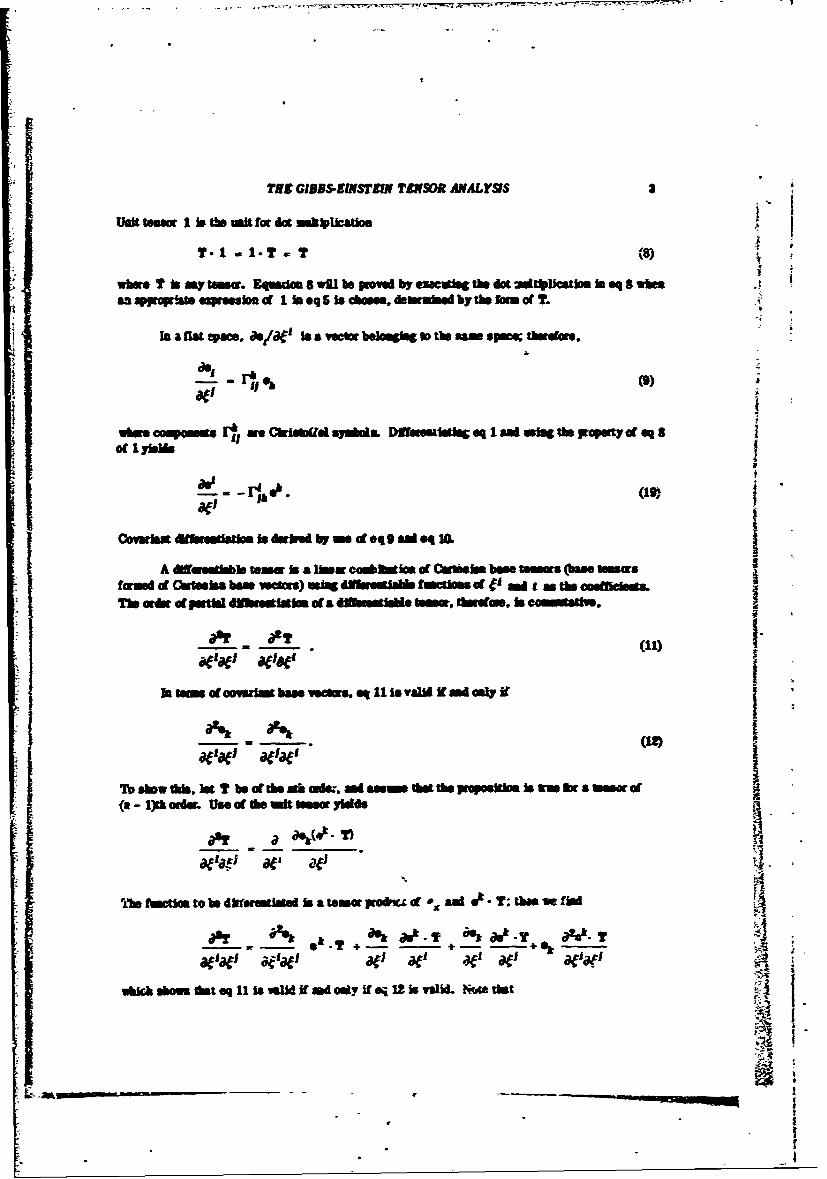
Limi oin" I is do mu tfor dot WRIaUton

T- 1~ -a.T -T(8

wlwe T b mnywmow. Eqrndma wIlbe poved by esuft the dot ati1JcsZi In eq 8 wbesa affwopim ipesin f In meq IS is~ o SUISS ea dm y th omE of T.

In a ilas epam, a./ae' is a weftrbelogims the rsam*o :brteb

(9)

wt mompancsr arcklowd sda DINffaei o~ q 1 a ftmis bpmiy Meq

coyarim asowam is ft by c.q 9 md 04 As

A mUims ffootabt is a Unar c4o~mbicf Cuoi base twms (bae umnsfamed d Cuseis bern wesms) utft dfemW" fmms of f, ad t as ti mnThe orft stpwtb d~megigam of a diaetiMe hmSIft m. ft cm~siv.

ft ifmatcoysglinbass Wcsm 0% Itisyaw K d adit

at

To show dds. Ist T be ct tb he m ds. sed sme dot ths aPoqsMidm ft WW ab f r of

(w-1~boid. Us~atebit - T)~d

aflaf' ar9 ar,

xLo tiniamto be dbfmnios bs a team p,* of a d s.- T: thus w fim

a~aee aeaC at,1 WOO&

n busat q 1 vlidui~f md oiyI 2is vid. Nw rthat

4 THE GiBBS-EINSC'EIN TENSOR? ANALY$,'S

... = e (13)

where B6 is a component of the Riemann-Chrjtoffel tensor. IThe nabla operator / is defined by

'V = 'I 1 (14)

Nabla q invariant under coordinate transfor-i-,,s; aerefore, it is denendent on time t only.

The gradient of a tensor T of any order is definee '

grad T = a (15)

where e i is usually put at the eitreme left of the base tensors oi Mde', but may be put anywhere

in the base tensors of aT/a to form a tensor of one order higher than T.

Divergence of a tenor T of nny order is dMined by

div T = *jc• '! (a6)

where @I is usually dotted with tih base vectors at the left ends in the base tensors of ol/aei,

but mz:y be dotted with any base vectors in the base tensors of aoTia lf to form a tensor c one orderlower than T.

Cwlo f a tensor T cf any order is defined by

crX, T = . x __ (17)

where ei is usuaily crossed with tue base vectors at the left ends In the base tensors of W,/fl

but may be crossed with any baae vectors in cT/Oe to form a tensor of the same order as T.

The use of nala thus introduced allows us to extend use of almost all the integral anddifferential vtctor formulas to a tensor of any order in the Gibbs-Einstein expression (Takagi, 1968).

Time differentiazion keeping f I, e, e3 constant is denafed by D/At. Thus,

Di

V (8

Differentiating eq 18 with respect to , yields

De1 _oV 19• 0-V

THE GIBBS-EINSTEIN TENSOR ANALYSIS 5

The symmetric part of grad v is denoted lb'

(gad y)l - ill* (20)

Component8 1 1 satisfy

21l gi (21)Dtj

Strain tensor a is given by

£ f~ ~ dt (22)

where 91 is the initial value of e and in ct dependent on t. When the deformation is the elonga-tion of eI, or08•. the integral

fo e j*lo dt (23)

whose inteprand is a product of three time-dependent functions, yields a logarithmic strain. Ingeneral, however, the integral of eq 23 is depuident on the path of integraton (Yoshimura. 1957).a may be shown by following elongations and rotations in different orders, and therefore is not athermodynamic stAte variable. a in eq 22 is a thermodynamic sta variable representing a thermo-dynamically reversible process (see the end of this part).

Note that

= ~ (24)a1 2

where the numbers and letters unde, the tensor symbols indicate identical base vectors when theyare on different sides and base vetors to be dotted when they we on the same side. The quantity'n the brackets is a scalar product c deloruatiou dyads, .i3 and . which define the inversedefaratioa from time t to time t = 0, To show this, let eldel be a material point in the neighbor-

hod of a particle whose material bases are o, eI at tim t and 0 , e at time t = 0. Dotting

o1df from the left in el 0 yields Ode 1. Therefore, dotting from the left in Wo is equivalent toa deformatm.i changing eidfl to sod i . In Part 1I, the more realistic interpretation of deformation

dyads will be given.

Three vectors e (i = 1, 2, 3) o f 1, S 2, f3 in a more-than-three-dimensional space span three-dimensional subspace, letting ' e2, be a set of curvilinear coordinates of the subspace, ifand only if esdf 1 and (de/064df are total differentials. The latter condition, which yields thecompatibility equations of components i, requires that dei must be a linear combination of vectors ,! •

Sand therefore shows that the space spanned by vectors e# is flat.

_

6 THE GIBBS-EINSTEINI TENSOR ANALYSIS

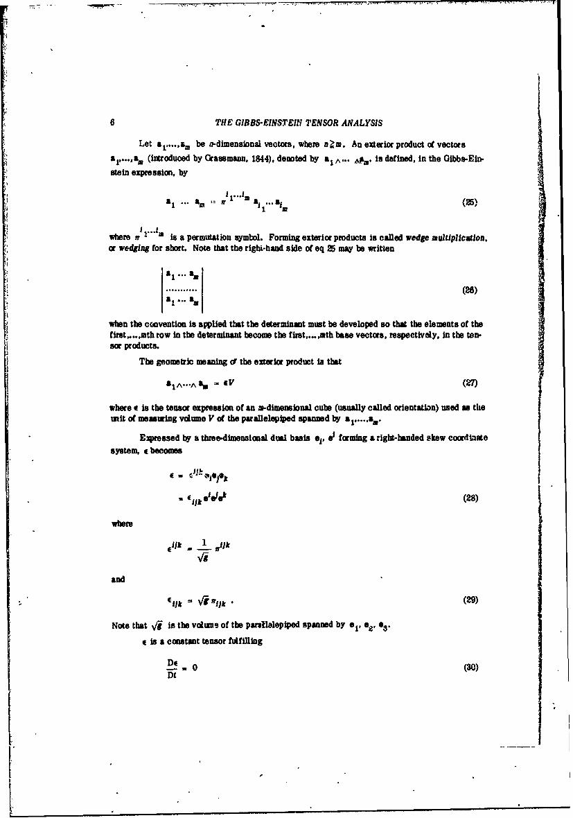
Let am be n-dimensional vectors, where nIm. An exterior product ol vectorsa~..a(introduced by Ckassmann. 1844), denoted by al A Alta, is defined, in the Gibbs-Ein-

stein expression, by

ra ... (25)

where rr is a permutation symlol. Forming exterior products is called wedge multiplication,or wedging for short. Note that the right-hand side of eq 25 may be written

.......... (26)

when the convention is applied that the determinant mut be developed so that the elements of thefirst,..,mth row in the determinant become the flrst,...,mth base vectors, respectively. in the ten-sar products.

The geometric meaning of the exterior product is that

ZIA ... AaM-G (27)

where e is the tensor expression of an a-dimnensional cube (usually called orientation) used as thenit of measuring volume V of the parallelepiped spanned by

Ezressed by a three-dimensional dual basis ej, @I forming a right-handed skew coordinatesystem, a becoms

AE = q

. 9 ilk 91016k (28)

where

ilk _1 ilk

and

ilk N41"hlk .(29)

Note that Vrg is the voltue of the parelleleplped spanned by e 1,02 03.

G is a constant tensor fullling

Dr6 0 (30)

F -t


and

dE 0. (31)

Similarly to c, 1 is also a constant tensor fulfilling

D = 0 (32)DL

and

.2' = 0. (33)

An n-dimensional cross product may be defined by dotting with the n-dimensionals

i~ 2 i3**i nf• Ab a cl.. t b a 3...e

.n (34)123...n 12 3 ... n

where E..i is acomponent of the n-dimensional E. Because of the antisymmetric properties

of a, there we many other choices of dotting base vectors in e in the left-hand side that yield thesame result as in the rigt-hand side, which, however, need not be shown here.

The exterior differentiation (introduced by Cartan (1922)) of a tensor T of any order is given,in te Gibbs-Einstein expression, by

0 A (35)

where e i is usually wedged with the base vectors at the left ends in the base tensors of oT/d',

but may be wedged with any base vectors in the base tensors of aT/f' to form a tensor of oneorder higher than T.

The amisymmetric part of the three-dimensioml gradient of v is equal to

(pad v]A =W ^

The following remak shovs that a material symmetry that existed at time t =0 exists

throughout the deformation.

Denote 11 00 and the base vectors ad a vector at time t 0 respectively,

= e ° (37)

8 THE GIBBS-EINSTEIN TENSOR ANALYSIS

where scalars ai are components of a referred to At time t, | and become e| and a,respectively, but the components ai are the same,

a = ale. (38)

0

Proof. Let initial coordinates if different from iodefine fp and fp different from e,and ei, respectively. Then we have

= fpd7 p (39)

at timo t and

e, df 1 = fpdiP (40)

at time t - 0. Therefore, the transformation from e, to fp is the same as the transformatiou from

to

Letting & and a be one of fo and ft, respectively, proves the theorem. The proof is thus

completed.

The remark shows that constitutive equations must he written in terms of materialcoordinates.

Next, the axiom of objectivity will be given the Gibbs-Einstein expression. Let ca - da

be a net of fixed orthogonal vectors and aa(t) = a(t) be a set of moing unit orthogonal vectors.Define

Q a = aac. (41)

12 12 12

The inverse of Q is

QI= T =Cadm = a (42)12 12 12 : 2

because they satisfy the relation

Q.Q- Q - .Q= 1. (43)la a2 la &2 12

A rotation that changes x = 0ca to y = r0aa is given by

y = Q.x= x. QT (44)

where nothing is shown under tensor symbols on the convention that two base vectors adjacent tothe dot, one on the left and one on the right, shall be dotted when no indication for dotting isgiven.


Define

y= Q.z+bt) (45)

where b(t) is a function of t. Vector x is referred to the fixed coordinate i spanned by ca ,

and vector y is referred to the moving coordinates rotating with aalt) sd translating with b(t).

Let i be a functionof a and t, and define

S=7.y. (46)

Then we find

d, Qo . e, .QT

91 = QT.di = di'Q

(47)

df @Io qT, q 4

Of 1 0 1 Q QT 1

Let

Dy a.. (48)

Then, oparating D/Dt on y in eq 45 yields

.DQ DbQ-v+ .+ (49)

The nabla of u in the moving coordinates is given by

di o f. QT (Q. v DQ \\~ ~L Dt )

a b 1 ia b2 2 b2 2

SQof_ .QT Q.DQT

S(Dt50)

a1 1 2 2b aI lb

Similarly, we find

a d d Q a.v *I . QT PQ Q (51)

ab at 1 2 2b &I lb


Adding eq 50 and eq 51 yields

di 0 + I di .Q. ei I V +N IV ei .QTde -- Q. * + • (52)

which shows that (grad v)s is objective. Subtracting eq 51 from eq 50 shows that [grad V]A isnot objective.

Base vectors a, , e| are objective as shown in eq 47. An objective second-order tensorsatisfies

T = eiT 1ej . dShkdk (53)

where Shk is the components in the moving coordinates. Operating D/Dt on T in eq 53 yields

DT = (D- + TO l + TiPv (54)

which is again objective.

a in eq 22 is a thermodynamic state variable reprsenting a thermodynamically reversibleprocess. To explain this, we first notice that dU, for example, in thermodynamics may be identi-fied with (DU/Dt)Dt. This recognition leads us to a thermodynamic principle: A thermodynamic

function U, for example, is a function of quantities qi, if DU is expressed as a linear combina-

tion of Dq1 when quantities qi are independent with each other.

From thermodynamics,

DU = DQ + DW (55)

where U is the internal energy per unit mass, and DQ and DW are heat and work inputs, respec-tively, per unit mass per unit time. Divide DW into two parts

DW = (DW) rev + (DW)'f v (56)

where (DV)rev and (DW)ilr ev represent reversible and irreversible work, respectively. Then wehave

DU TDS 1-(DWIV (57)

TDS DQ + (DW) itre v (58)

where S is the entropy per unit mass.

When body couple and couple stress do not exist in the continuum under consideration, wehave

(DW)T ev : l oDg1i. (59)

2o


Therefore, U in eq 57 is a function of gs, t, an.1 S. Because g,, is a tensor component, we may

consider 9,,&' as an independent variable of U, where the Gibbs-EinsteMn expression of eq 59

.DWfev %O q.D(5jjW) (60)

la ab b2 12

is considered, in which a is expressed with current base vectors. (The author was encouraged touse the expression on the right-hand side of eq 60 by Mindlin and Tiersten (1962).) a in eq 22 isintegrated to

= 8 - 1) (61)

where gl t" and 1 is contant tensor.

PART i. CANONICAL FORM Or GNERAL 8ZCOND-ORDUIT tENSORS

The Hamilton-Cayley theorem in matrix theory is given che Gibbo-Eiustein expression in the

following. As shown below, the dual basis expression is more than suitable for discussing thecanonical forms of general second-order tensors.

Firet, to give a summary of this part and to show how the resdits my be ubed, the resultswill be applied to three-dimensional tensors. Canonical forum of not necessarily symmetric realthree-dimensional second-order tensors in the Gibbs-Einstein expression are ciasified into fourcategories:

Category 1: Eigenvalues A ( = 1, 2, 3) are all real, and determine three pairs of left and Mghteigenvectors which are never orthogonal with each other. Then eigenvectors span a dual basis

ei , ei satisfying

T Aje 1 (62)

T. e , A1el (63)

where , =,2, 3. The summation convention is not applied on the right-hand sides. Juxtposing

• t from the left in eq 62 aW s, from the right in eq 63 witb ine summation convention appliedyields the same expression

T 3 i ee (64)itO

which is the canonical form of category 1. Note thatteigenvectors are not necessarily unit nororthogpnal. When e = eligeuvectors are unit orthogonal and T is symmetric. Elgenvalues in

category I may be multiple roots.


Category 2: k 1 is a double real root which determines an orthogonal pair. An orthogonal pair isa pair of left and right eigenvectors determined for an eigenroot and orthogonal with each other.

Choose e2 and e as the left and right eignvectors determined for A,- then

•2 * T = A10e (65)

T.e = A ei. (66)

Let X2 be the remaining real eigenroot, and e3 and e3 be the left and right eigenvectors, respec-

tively; then,

e ' T - 2 3 (67)

T • 3 = A e3. (68)

As proved later, e1 and e2 can be chosen to satisfy

•0*T = A(e1 + ) (69)

and

T 0 e = X(eI + e2). (70)

Juxtaposing •1, •2 . • 3 from the laft in eq 69. 65, 67. respectively, and summing the results, andjuxtaposing o,, •2 , 03 from the right into eq 66. 70. 68, respectively, and summing the results,

yield the same expression.

T = k1(616e +e20 + ele 2 ) + A2ee3 (71)

vhich is the canonical form of category 2. The canonical form has one off-diagonal term A1e 1a .

As shown later, choice of base vectors for expressing the canonical form in category 2 is nottunique.

Category 3: A is a triple real root which determines an orthogonal pal. Chose e8 and •

as the left and right eigenvectors determined for A; then

•3 -T = Xe (72)

T-e I = As'. (73)

As proved later, ei , e 2. e2 and @3 can be chosen to satisfy

•1 . T = A(@1 + e 2) (74)

a2 - T = A 2 +0 3) (75)


T s 2 = A,(61+e02) (76)

and

T-e 3 = (e2 +e 3). (77)

Juxtaposing e., e2, e from the left in eq 74. 75. 72. respectively, and summing the re-sults. and jaxaiosing si, , 2 , from the right in eq 73. 76, and 77. respectively, and summing

the results, yield the same expression.

T = Metes + Ole 2 + 3 (78)

which is the canonical form of category 3. The canonical form has two off-diagonal terms. As 102

and Ae2 e3 . As shown later, choice of base vectors for expressing canonical foram in category 3is not unique.

Catqory 4: Two eigenroots are conjugate complex. As shown later, eigenvalues and eigenvec-tors in this case are expressed as p(oos 0 T j sin0) and ea t is2 , e T j@2 thus we find

( I t*2) • T p(cos0 t isin0)(e I _ j02) (79)

T • (e I . ie2 ) p(cos 6 i i )sin8)(e I ie 2) (80)

where 0, e .ao1 •2 are real vectors, and p and 0 are real numbers. Decomposing eq 79 and 80

into the real and imaginary parts yields

• T = p(e 1 0s0+ e 2 Zin0) (81)

a • T - p(e 2 Cos 0- aelsin 0) (82)

T - *I - P(01 cose - eesine) (83)

T • 02 - P(ecos 0+ t sin ) . (84)

Let p be the remaining real eienroot and e..03 be the left and right eigenvectors, respectively;then.

• 3 .*T - jre3 (85)

and

T -9 3 . /e 3 . (86)

Juxtaposing et, •2. •3 from the left in eq 81. 82. 85. respectively, and summing the results, and

juxtaposing a, . • 2e . s3 from the right in eq 83. 84, and 86. respectively, and summing the results,

yield the same expression

14 THE GIBB-S-EINSTEIN TENSOR ANALYSIS

T - p(ee + e 2eo,)Cos8 + p(ole -0 21)slno+# &08 , 17)

which is the real canonical form o category 4.

A general second-order tenr T can be witten as a dyad T - albi and may be interprtedas a de(ormation dyad. Interpreted this way, the equations in eq 62 show that elongagioms in threedkections e, e 2. and e3 have occurred. Equation 6P in category 2 shows that a slip has occurred

in the *1. e2 plane along the e. axis. Equations 74 and 75 in category 3 show that a double slip

has occiired in the e 1 , 0. plane along the e 2 axis and in the e2, *, plane along the esais.

Equations 81 aW 82 in category 4 show that a rotation by angle 0 has occurred with *3 as theaxis of rotation.

C..plex teears

In the following sections. general a-dimensional second-order ten~ors are given canonicalform. For that ve must fist extend theory of real tersors to theor of complex tenors.

A set of unit orthogonal vectors ca - (a -... ,) is fixed in te space ad used as he

itaard of the coordinate systems. Vector

v = v c% (88)

is called a complex vector f componts. v a (a - 1,....n) in the standard epremion (eq 89)

are complex numbers. Conjugate v of v is defined by

v-pc .(89)

Detting (T) complex vectors a with v. denoted by a : Y. is defined by

e r-e a . V (90)

where dotting (-) o the right-hand sie is the dolaig in real Euclidean geometry applied to complexvectors. Vector v satifyig v - v - 1 is said to be of uit length. Vectors a ad v Satisfyinga : v = 0 or v: - 0 we said ID be atbogool A dul basis,.e. e for complex wctrs satisfies

e . 8),,a (91)

or

of.. (a

where 41 and are Kronecker deltas.

The utandad exression of an L-dimensional complex secood-order tenor T is defied by

T Tfiel (93)


or

T T'- 1 (94)

in which the first and second members of the dyas are with and wiloit Ode. respectively. andi-1;...*. The stndadx fom of a comqlet vector is given by rsing bs vectrs witout tilde.

v - a'oh (9)

or V - VO . (96)

Vec&o¢ vin eq and 96 can be eadly dotted (-) fr,.be left i ',oT c(eq 93 and S4.respectively.

In the foilowicg. we. wil derive equations loy which a no-stand d epressin is trans-

fbmd to a maud ezpesson. DefJze and J] by

ell= *I (97)

sod

~!O'SI(91S)

respectively.Sj L Inala. The Wit W or lis gives by

t- I - ;, (I0is e¢)ad satiufies

t -1V (0)

Ore is m Shrimy Vector.

LOOM lb

o0 ,H (101)___ _ _


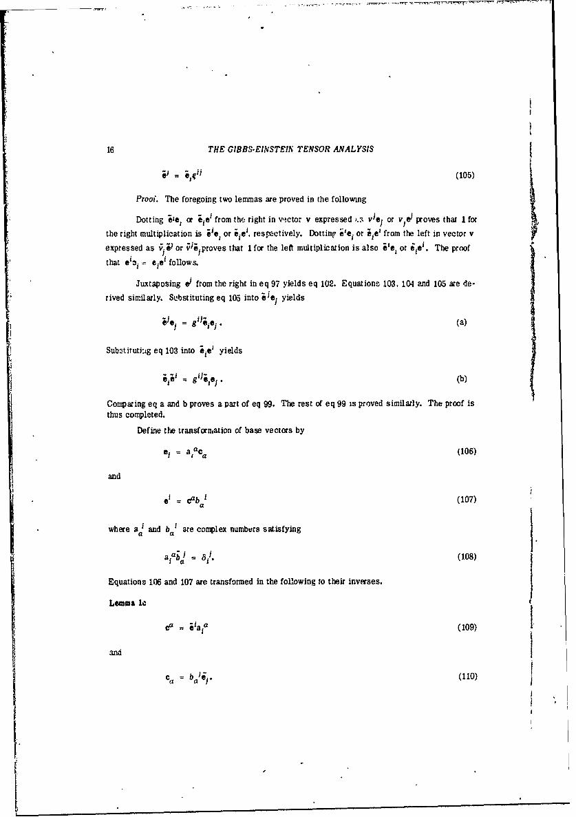
= (105)

Prooi. The foregoing two lemmas are proved in the following

Dotting ;'e, or eie' from the right in vctor v expressed , v~e. or v e) proves that I for

the right multiplication is Ve, or ;ie', resectively. Dotting i'e, or il from the left in vector vexpressed as iV or ',proves that I for the left multiplication is also ;1e, or iie'. The proof

that = i = eyei follows.

Juxtaposing ei from the right in eq 97 yields eq 102. Equations 103, 104 and 105 are de-

rived similarly. Substituting eq 105 into ;Jye yields

ie ie = gi] iej. (a)

Sub-tjtutj:,g eq 103 into ;ee yields

9 ie = Is (b)

Comparing eq a and b proves a part of eq 99. The rest of eq 99 is proved similarly. The proof isthus completed.

Define the transformation of base vectors by

ei = alaca (106)

and

a' = raba (107)

where a. and ba are complex numbers satisfying

aaj 8 a. (108)-~ a i.08

Equations 106 and 107 are transformed in the following to their inverses.

Lemma lea a (109)

and

a(

r "

TUE GIBBS-EINSTEIN TENSOR ANALYSIS 17

Proof. Dotting cP into eq 106 yields

a1P = -C . (a)

Juxtaposing from the left of eq a yields eq 109. Equation 107 transforms to eq 110 similarly.

Theorem I

ei = aia b% 0 (li)

= eJaa'b'. (112)j a

Proof. Substituting eq 110 or 109 into eq 105 or 107 yields eq 111 or 112, respectively.

Corollary I

= aiah e. e (113)

fa a e,

e = e l jabai (114)

Proof. Taking the conjut.tes of eq 111 or 112 proves eq 113 or 114, respectively. Theproof is thus completed.

Equations. 111 through 114 me the equations that must be used to transform non-standardexpressions to standard expressions.

Kigenvectorks and eigenvalues

Let T be an n-dimensiona!, tensor in the standard form. A left or right eigenvector of Tis an n-dimensional complex vector x or y such that dotting (.) x or y from the left or right in Tyields a vector in the direction of x or j, respectively; that is

z. T . Ax (115)

or

T -- A (116)

where A is an eigenvalue.

Let T ard a left eigenvector x oe expressed as

T Tj a e, (117)

and

x - xhh (118)

respectively. Substituting eq Ili and 118 ;nto eq 15 and equating thv components on both sidesof the transforme "' equation yields

18 THE GiBBS-EINSTEIN TENSOR ANALYSIS

xii . (119)

Let a right eigenvector y be expressed as

y = yhe (120)

Substituting eq 117 and 120 into eq 113 yields

T1' -- = A" (121)

Equations 119 and 121 determine the same characteristic equation

T - I = 0. (122)

Therefore, ooe A determines at least one left and one right eigenvector. The rank of matrix

(Ti- A) will be cLUed the rank of root A. Solutions of eq 115 and 116 do not depend on the

choice of a type of T or of a dual basis.

Canozical forms

Lemma 2a

Let A and p be two different eigenvectors of T; let x and y be left and right eigenvectorsdetermined for X, respectively; and let u and v be left and right eigenjectors determined for ji, respec-tively. Then x and v are orthogonal.

X. = 0 (123)

and y and u are orthogonal,

y. 0. (124)

Proof. Dotting (.) from the right in eq 115 yields

x. T . - Ax- i. (a)

Dotting (.) from the left in the equation

T =

yields

zT. , = - x. . (b)

Because A+ by assumption, eq a and b are compatible if and only if eq 123 is true. Equation 124may be proved similarly.

Lemma 2b

If all the room are single, no orthogonal pair exists.

THE GIBBS-Fi NSTEIN TENSOR ANALYSIS 19

The netx lemma proves this lemma. Note that vectors e and a' forming a dual basis arenot ort hogonal.

Lemma 2c

Assume that n roots k..... Aa of the characteristic eq 122 are distinct. Then, T can be

reduced to the canonical form

T h5 o (125)

The rank of k(i= l .... n) is equalton- 1.

Proof. Each A, determines at least one left eigenvector. Let e, be the left eigenvectordetermined for A( = n)

6 * T - A1e1 (a)

on - ",. (b)

Form a dual basis e, 91 (I = 1l...n). Justapouing ..... from the left in eq a,..., eq b,

respectively, and summing the result yield eq 125. Dotting (.) e' from the right in eq 125 shows

that a' is a right eigenvector determined for hi(i - I,-, n)

T in eq 125 shows that each k, determines one and only one pair of left and right eigen-

vectors. The rank of the roots is therefore all equal to n - 1. The proof is thus completed.

A multiple root which determines fewer eigenvectors than the number of multiplicity of theroot is said to be singular.

Lemma 2d

At least one orthogonal pair belongs to a singular multiple root. If more than one orthogonalpair belongs to a singular multiple root, the number of orthogonal pairs can be reduced to one.

ProoL. Assume that eigenvectors x and y determined for a multiple root are not orthogonal.

Then, we can choose e= x and e° y after, if necessary, changing the lengths of x and y to

make z : y - 1. Then we have

6.1 T X61 (a)

and

T~ - (b)

Form a dual basis eP ei (I 1 ... ,n) by introducing a certain number of base vectorsthat are

idependent of e, ea aid each other; express T with the dual basis'9 r , °.

______ -- sr-- -° - - - - .... ; /

' v -. ,- . , .. ,


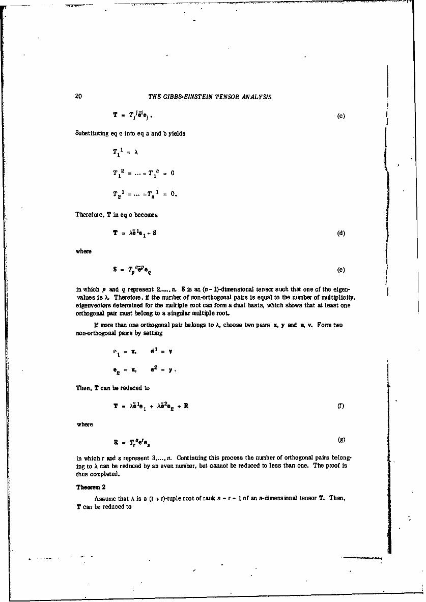
T = TO'e,. (c)

Substituting eq c into eq a and b yields

T12 Til 0

T 2 -T'=0.

Therefore, T in eq c becomes

T = A e1 +8 (d)

where

S = TppDeq (e)

in which p and q represent 2,.... n. 8 is an (n - 1)-dimensional tensor such that one of the eigen-values is A. Therefore, if the number of non-orthogonal pairs is equal to the number of multiplicity,eigenvectors determined for the multiple root can form a dual basis, which shows that at least oneorthogonal pair must belong to a singular multiple root.

If more than one orthogonal pair belongs to , choose two pairs x, y and u, v. Form twonon-orthogonal pairs by setting

t"1 = x, l = V

02 =U, e2 =

Then, T can be reduced to

T =A Is + A 2e2 + R (f)

where

R = TSre. (g)

in which r and s represent 3,..., n. Continuing this process the number of orthogonal pairs belong.ing to A can be reduced by an even number, but cannot be reduced to less than one. The proof isthus completed.

Theorem 2

Assume that A is a (t + r)-tuple root of rank n - r - 1 of an n-dimensional tensor T. Then,T can be reduced to

______I


T = A(Ile I + .,. + ' i- + + + ;". + a1+ 8 (1mI)

where 8 does not have X as an eigenvalue and is (n - t - r)-dimensional. Then, the left eige.a-vectors determined for X are • 1 , t+ .... t0, The rigit elgenvectors determined for X are

t, . Vectors 02 ... t Stisfy

T = Ae6 + .-1 (127)

where 4 represents t - 1 integers

2 5 q5 < t .

Vectors e....,e-1 satisfy

T. e = Ae q + e' + 1 (128)

where kb represents t - 1 integers

l< ,<t-I.

The number of off-diagenal terms is t - I.

Proof. Because the rank of A is n - r - 1, (r+ 1) pairs of independent left and right eigenvectorsexist, of which, if C-5 2. one is an orthogonal pair. Denove by oil ' the orthogonal pair, by

ll.... the left eigenvectors, and by a , at + r the right eigenvectors. Then

*rlT = ko1 (a)

lit+l'-T = et+lI (b)

OWr T X et+r (C)

T. : AWt (d)

T- = A;' +1 (e)

T.- ;t r At*. M(f)

Form a dual basis *,, a' (I = 1,...,n) by arbitrarily introducing independent vectors e2..'e t ,

........e ..... e- etr..... e* . Express T as

T = T' 1 ei (9)I I


Substituting eq g into eq a thr~nugh f yields

T i As I (a,)

Tt+1j At+1j(l

Tt~rj a ~r r(c')

t= a t(d')

T, +1 = j At+1 (e I)-

T t+r = ~Lr (f)I

The matrix of T - X1 is shown in Figure 1, in which all the elements on the straight linesare zero, submatrix A is composed of 2rxd,..., tth row and 1st,...,(t - l)th column, and the maindiagonal of A is not on the main diagonal of the matrix of T - Xl.

Define x for a given vector a by

x -T = Ax +a. (h)

/0 -- 0-0-0-0----- - 0

tA CJ

f1 0- - -0-0-0-0 .- 0i_ _ _ _ I I I I _ _ _

0 0-0-0-0- 0_ _ _ _ 1 1 1 1 _ _p0 0-0-0-0 0

f. 0--0 -0

D8I

Figure 1. Matrix of T - Xl.


Equation h becomes

x(Ti- i) -a' (.)

by substituting eq g for T, eq 118 for x, and a aJof.

Because of conditions in eq d' through fl, equations in eq i are simultaneous n - r - 1equations given fori l ..... t-1. t+r+1 ... ,n. Vector a must satisfy a condition that componentsat ..... a4 r are zero. Because of conditions in eq a, through c', equations in eq i have n - r - 1

unknowns A.. xt, xt r+ I#.... xn . The determinant of the simultaneous equations (eq i) is ofrank n - r - 1, and is the only non-zero (n - r - 1)-dimensional submatrix containing A. Then x

* is determined with (r + 1) arbitrary components x , xt+ I.... xt'r.

Put a-0e and define x2 by

x2 T = kx2 +e I . (j)

x2 is linearly independent of e. To show this, define

Y = ylel + y 2X2 (k)

We find

y . T ky + y 61 (1)

by use of eq a and j. Therefore, if y 0, we necessarily have y = y 2 = 0. Let x2 be chosen as

new e2* Then eq j becomes one ct eq 127.

Put a= 2 and define x. by

X3* T = \x 8+02* (m)

x3 is linearly independent of e 2 and s 1, as may be shown similarly to the above. Let x3 be

chosen as new e3. Then eq m becomes one of eq 127.

Continuing this process, vectors 94, .,., e, are defined and eq 127 is proved. All the vectors

represented by e, in eq 127 satisfy the condition which must be satisfied by vectrc' a in eq h.

Suppose that eq g is expressed with the new base vectors thus introduced. Substitutingeq b thus determined into eq 127 shows that matrix A in Figure 1 is a unit matrix and that sub-matrix C in Figure 1 is a zero matrix, yielding eq 126.

Dotting (.) iO from the right into T in eq 126 yields eq 128.

Substituting eq g into eq 128 shows that submatrix D in Figure 1 is a zero matrix. Theproof is thus completed.


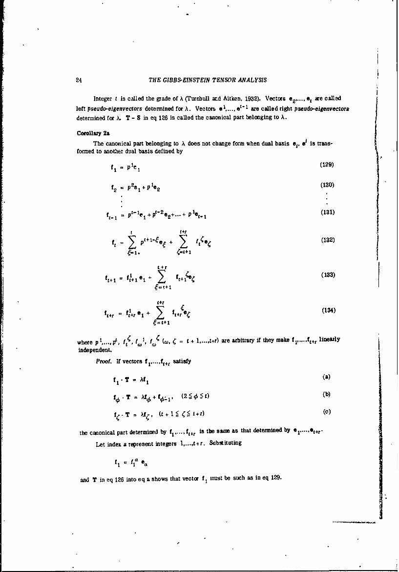
Integer t is called the grade of A (Turnbull acd Aitken, 1932). Vectors o2 ..... 0 are called

left pseudo-eigenvectors determined for A. Vectors o .... e- 1 are called right pseudo-eigenvectors

determined for k T - S in eq 126 is caled the canonical part belonging to A.

Corollary 2a

The canonical part belonging to A does not change form when dual basis e, 01 is trans-

formed to another dual basis defined by

fl = Plel (129)

f2 = p29 1 + p ie2 (130)

ft- I = p- e + t-22+... + p et- (131)

t t+r

ft P'+I4*o + I (te 132)

t r

f ft1 1 a1 4 ft+lSC (133)

t+r

ft +r alr 1 + I f t + (134)ft ~ ~'r tt+ I1

where p . p, ti.), tj (w, = t + 1,...,t+r) are arbitrary if they make t1 ,..... fJW linearly

independent.

Proof. If vectors f. ... ft+r satisfy

T M1 (a)

2= + 1, < (2€ :5 t) (b)

f 4 .T = Af, (t+1: <t+r) (c)

the canonical part determined by fl... ft+ is the same as that determined by 1 .... *t+r

Let index a rereselt integers 1,...,t4r. Substituting

f = fla

and T in eq 126 into eq a shows that vector f1 must be such as in eq 129.


Susbtituting

and T in eq 126 into eq b yields the conditions,

I0

which show that vectos f2..... ft must be such as in eq 130.... ,eq 132, respectively. Substituting

awl T in eq 126 into eqc shows that vectors tr.. . ft~1 must be such *a in eq 133.....eq 134.The proof is thus completed.

Corollary 2b

Left and right sigenvectors determined for a single root are not orthogonal.

Proof. Denote by 8 the sum of all the canonical parts belonging to the multiple roots. Then,

all the elgenvalues of T - S are single, and, as proved by Lemma 2b, no orthogcnal pair exists for

T-S.

HasMltm-Cayly TheomLemma S

Let 1..... * be a independert vectors and 8 be an n-dimensioaal complex tensor of any

order. If the relation

e• - = 0 (135)

is true sor all .e f l....,), then 8 is identically equal to zero.

Proof. Form a dual basis eJ. e'. Juxtaposing e i from the left into eq 135 and summing

over I yields the required property of S. The proof is thus ccnpleted.

Let T be a complex second-order tensor in a .ndad form

T = el Te (138)

Then, m time scalar product of T

T. • T To (137)


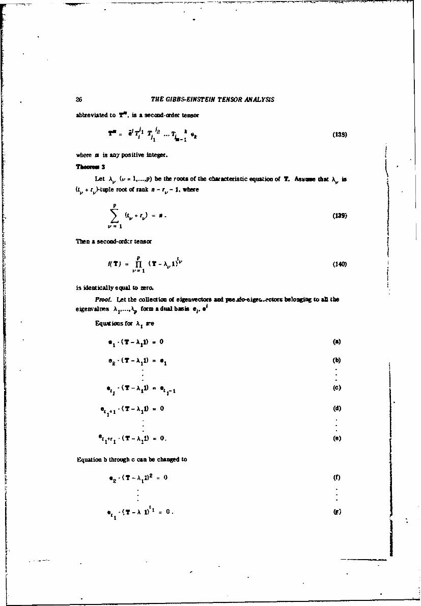
abbreviated to Ti. is a secmd-order tensor

T J '" 2 .- 1 k (13s)

where m is any positive integer.

Thsoe 3

Let AV (v 1,...,p) be the roots of thbe characteristic equation of T. Asv that AV is

(tv + rQ-tuple root of rank n - rV - 1. where

p

(tv + rV) = B. (39)

Then a secoed-ordcr tensorP|

I(T) = (T- 1 , (140)

is identicaly eqal to zero.

Proof. Let the collection of eigeeivectors and pe.Mo-eie-.Lctrs beonging to afl the

eigenalmes A1 ..... , form adualbasis ej. ei

Equations for A, re

el -(T -All) = 0 (a)

e -(T -Ail) = et (b)

* " (T-Al) = e -1 (C)

t 1+,-(T- A) = 0 (d)

et + •(T-A .) = 0. (a)

Equation b through c can be chaned to

( *(T-A 1A = . (I)

O 1

THE GMBS-EINSTEIN TENSOR ANALYSIS 27

Tlurafate. we find

ee - fAl))'l 0 (b)

elor

Sialady, we tiam

Form I(T) in eq 12. The Order of dottiag is eq 132 way be excbanged. because thefe

**sa of dWa in Menfoa orders we the sam. We tbudfe tied

AM = 0 U

wheI 1,..Tbn. I(T) min be Wee'tically eqal to into. The n o is tbis COWIeled.

poIymm"t I(x) obnaiwd by subsiaing ucal z for T is Own miniml polyuomia defiNedfur T.

Red mdnnul bum ofd eltomms

A 99MM is said to be Meal It tdnt exiss a VZOaf-35gis that chAnges niM teCOoMuCSto real a ' i and all the base veat o real vecors at lbe same tino. IS the tOUkwMgt. T isa necont-order teamo Ow bas real congoneats ad real ban vectors.

It is obelin that a rea] eiemvabie of T datemiae redlegavcos and that coliqaescompiez eilenva or T decmn coajegste coules eipavectars. Only lbe latter case needbe d~i~zew

Aammwn tka ifl wev (C + r)-toe roots ot rank n - r -1I of a real second-arder tessoir T.

At + ) =< n.

Tbn. T cm be reduced %D

28 THE GIBBS-EINSTEIl TENSOR ANALYSIS

2(t+r) t+r

T = a & + (f2qf ' - f 2 Q1f 2 q) +

+ ' (f2 f 2 + f20-1f 3 ) + S (141)

where f., I[1 _- p 2(t+r)] are real vectors, forming a dual basis, and 8 dces not have a±iO

as eigenvalues and is 2(n - t - r)-dimensional.

Vectors p, fP (p = 1,..., 2(t+r)) satisfy

fl'T = at,1 f2 (142)

f2 " T = af 2 + Of, (143)

f29-1 T = af 2951 - Of295 + f20- 3 (144)af+ f2 ~. 1 + fb- (2= 6 q 0 (145)

f 2el I . T = at 2e_ - 13t26 (146)

f2 e" T = at 2e+ pf 2e-'l (t+1 e:5 t+r) (147)

T • f2,- = af 2Y-1 + Af2 y + f2 + 1 (148)

T. f2y = af2y _ ptfy-1 +f 2 +2 (1: < : <t-l) (149)

T . f q-1 = af2q- 1 +,f2f7 (150)

T- f" = af29 -f27-1 (t < 17 < t+r). (151)

Complex vectors I (fq-1 ± i29 . (f2q- 1 T i1 2q) (q = 1,...,t+r) form a dual basis.

Proof. Let er.... eLr be complex eigenvectors and pseudo-eigenvectors belonging to

e ++

e, T (a + i3)0 1 (a)


e 2 T = (a + ij)e 1 (b)

• t T = (a + ip)e+et (c)

et+ = T (a + ig)et+I (d)

et+ r T = (a + iP)et+r. (e)

Write eq(1 q t+r) Vith real vectors f2q - ( 2q as

I1

q =- (f2q-l + If2q) " (f)

Substituting eq f into eq a through e yields eq 142 through 147.

Determine fP[ 1 <p < 2(t+r)] to form a dual basis tp, fP. Juxtaposiag f1,...,f2(t+r) from the

left into eq 142 through 147. respectively, and adding the equations thus formed yield

T = f(af1-1Pf2 ) + f2(af 2 +1f 1 ) +

+ t [f20-1(Wt _,3f2 + f2 3 ) + ,2S6 ('f2S6 +le 21 + f2 ..2 )] +

+ t [f2" t2(a£ - C-Pf2 )+ f2f (af2 +if, t) +S (g)

where S does not have a ± ip as eigenvalues. T in eq g can be transformed to T in eq 141.

Dotting fi .... f2(t+r) from the right in T in eq g yields eq 148 through 151, respectively.

The proof is thus completed.

T in eq g may be expressed as

f

T = S+ (fl ... f((152)

12(t ( r)]

where T is a 2(t+r) by 2(t+r) matrix

in which A is a 2t by 2t matrix

•30 THE GIBBS-EINSTFIN TENSOR ANALYSIS

a -A 0 00 ...... 000 0

a 0 00 ..... 000 01 0 a -a 0 . 0 0 0 0

0 1 a 0 ..... 000 00 0 . 000 0

A . . . .

0 0000 . . . . .

0 0O0 0 0 .. . .. 0 1

B is a 2r by 2r matrix

a -9 o ..... 0 00.

-1,aO 000

OOa 000

B=

0 0 0 Oa-fi

10 0 0o a

C and D are composed of zero only. In matrix A, all the elements on the line parallel to the maindiagonal and containing 1 are 1.


LITERATURE CITED

Cartan. E. (1922) Lecons sur les invariants Intraux. Gautier-Villars. Paris: Hermann.

Gibbs. J.W. and Wil.s-n. E.B. (1901) Vector analysis. New York. Dover Publication-, (re-i publication. 1960).

Grassmann. H.O. (1844) Ausdehnungslehre.

llessenberg. 0. (1917) Vektorelle Begrundung der Dfferenttalgeomemne. Mathemati.vcheAnnalen. vol. 78. p. 187.

Mindlin. R.D. and Tiersten. H.F. (1962) Effects of couple-stresses in linear elasticisv.Archive for Rational Mechanics and Aaalysis, vol. 11. p. 415-448.

Sedi . ,... (1962) Introduction to the mechanics of a continuum medium. Reading. Mass.

Addison-Wesley. translation. 1965.

Takagi. S. (1965) Note for the lectures on tensor analysis conducted in the U.S. Army ColdRegions Research and Engineering Laboratory. from Apnl 196q. to February 1965(unpublished).

(1968) Unified treatment of vectors and tensors in n-dimensional Euclidean space.U.S. Army Cold Rerons Research and Enginee'ng Laboratory (USA CRREL) Re-search Report 207.

Turnbill. H.W. and Aitken. A.C (1932) An introduction to the theory of canonical matriees.New York, Dover Publications. 3rd edition. 1961.

Wills. A.P. (1931) Vector analysis with an Introduction to tensor analysis. New York:Dover Publications (republication. 1956).

Yoxhimura, Y. (1957) 3oxei-rikigaku (Theory of plasticity). Tokyo: Kyontsushuppan K.K.

Uncla ssifie dSecurty Classification

DOCUMENMT CONTROL DATA.- R &D(Secwt A.lc l,. ilber. bt.tadidzn aettlion must 6e entIered Whom me overall I.o to 1881104

I- ORIGIN4ATING ACTIVITY fCeEloe OW&t) 2d6 REPORT SECURITY CLAS9IFICATION

Cold Regions Research and Engineering Laboratory UnclassifiedU. S. Army Terrestrial Sciences Center $ rouJpHanover, New Hampshire 03755

8. REPORT TITLE

THE GIBBS-EINSTEIN TENSOR ANALYSIS WITH APPLICATION TO CONTINUUMf MECHANICS AND CANONICAL FORMS OF GENERAL SECOND-ORDER TENSORS

41. DESCRIPTIVE NOTES (y~pe f ti nd kebIi~Vedft.)

Research Report

Shunsuke Takagi

S. RE1PORT DATE 78. TOTAL NO0. OF PAGES 75 N. OF NEWSNovember 196"3 1

b.CON T *Ac r ON GRANT NO. 9s, OXIGINATOWS REPORT NuWOER901

6. PROJECT No. Research Report 221

C.b.O'.%KE REPORT Note) (AW 04WAN06ft 111tinap 89WDA Task IT06110ZB52AOZ a"Pn

10. OISTRIOUTION SIATIZUSMY

This document has been approved for public release and sale; its distributionis unlimited.

tII- SUPPLEM1EN4TARY NOTES 1.SPONISORING IWILITARY ACTIVITYCold Regions Research & Engineering

tI LaboratoryU.S. Arm errestrial Sciences Center

A nw tnso anlyiscaled heGibbs-Einstein tensor analysis, is developed basedon the concept that directions are algebraic quantities subject to the rule of formingscalar products, ten.4or products, and linear combinations. The mn-w tensor analysisis explained an this paper by way of reformulating continuum mechanics and theHamilton-Cayley theorem in matrix theory. The latter reformulation yields anexplanation of the de~formation dyads introduced in the former reformulation. Ascalar product of two deformation dyads yields the strain tensor, which is a thermno-dynamic state variable for thermodynamically reversible deformations. Mathernat-ics dealing with directions in a flat space becomes much simpler and more under-standable when the Gibbs-Einstein tensor expression is used.

1473P* UM U6 Unclassified

Unclas sifiedftcvItty classiftcaU

14. LINK A LINK 0 LINK CKEY[ W@O5~l

ROLE W? VOLSEr

WT ROLI[ WT

Tensor analysisContinuum mechanicsScalar productsTensor productsLinear combinationsMatrix theoryDeformation dyadsGibbs-Einstein tensor expressionGibbs tensor expression

Einstein tensor expressionHamilton-Cayley theorem

I!

UnclassifiedS c........ss.f...

Date post:	27-May-2020
Category:	Documents
Upload:	others
View:	20 times
Download:	0 times

THE GIBBS-EINSTEIN TENSOR ANALYSIS · the gibbs-einstein tensor analysis with application to...

Documents