The Hidden Beauty of Structural Dynamics -...

BUDAPESTUNIVERSITY OF TECHNOLOGY AND ECONOMICS

DEPARTMENT OFSTRUCTURAL MECHANICS

Robert K. NEMETH • Attila K OCSIS

The Hidden Beauty ofStructural Dynamics

Budapest, 2013ISBN 978-963-313-088-9

CONTENTS

Contents

Contents i

List of figures iv

List of tables v

Preface vii

1 Dynamics of single- and multi-DOF systems 11.1 Vibration of SDOF systems . . . . . . . . . . . . . . . . . . . . . . . . . .. . 1

1.1.1 Derivation of the equation of motion . . . . . . . . . . . . . . .. . . . 21.1.2 General solution of the homogeneous ODE . . . . . . . . . . . .. . . 41.1.3 Particular solution of the non-homogeneous ODE with harmonic forcing 71.1.4 Support vibration of SDOF systems . . . . . . . . . . . . . . . . .. . 11

1.2 General forcing of SDOF systems . . . . . . . . . . . . . . . . . . . . .. . . 131.2.1 Duhamel’s integral . . . . . . . . . . . . . . . . . . . . . . . . . . . .131.2.2 Numerical solution of the differential equation . . . .. . . . . . . . . 15

1.3 Vibration of MDOF systems . . . . . . . . . . . . . . . . . . . . . . . . . .. 181.3.1 Equation of motion of MDOF systems . . . . . . . . . . . . . . . . .. 181.3.2 Free vibration of MDOF systems . . . . . . . . . . . . . . . . . . . .211.3.3 Harmonic forcing of MDOF systems (direct solution andmodal analysis)241.3.4 Approximate solution of the generalized eigenvalue problem (Ritz-

Rayleigh’s method) . . . . . . . . . . . . . . . . . . . . . . . . . . . .311.4 Summation theorems . . . . . . . . . . . . . . . . . . . . . . . . . . . . . . .39

1.4.1 Dunkerleytheorem . . . . . . . . . . . . . . . . . . . . . . . . . . . .391.4.2 Southwelltheorem . . . . . . . . . . . . . . . . . . . . . . . . . . . .421.4.3 Foppl–Papkovichtheorem . . . . . . . . . . . . . . . . . . . . . . . .44

2 Dynamics of slender continua 462.1 Longitudinal vibration of prismatic bars . . . . . . . . . . . .. . . . . . . . . 47

2.1.1 Differential equation of motion . . . . . . . . . . . . . . . . . .. . . 482.1.2 Free longitudinal vibration . . . . . . . . . . . . . . . . . . . . .. . . 49

2.2 Free torsional vibration of prismatic shafts . . . . . . . . .. . . . . . . . . . . 532.3 Shear vibration of prismatic beams . . . . . . . . . . . . . . . . . .. . . . . . 55

i

CONTENTS

2.3.1 Differential equation of motion . . . . . . . . . . . . . . . . . .. . . 562.4 Transverse vibration of prismatic beams . . . . . . . . . . . . .. . . . . . . . 60

2.4.1 The equation of transverse vibration . . . . . . . . . . . . . .. . . . . 602.4.2 Free vibration of prismatic beams . . . . . . . . . . . . . . . . .. . . 632.4.3 Forced vibration of prismatic beams . . . . . . . . . . . . . . .. . . . 72

3 Dynamics of planar frame structures 813.1 Statical matrix displacement method . . . . . . . . . . . . . . . .. . . . . . . 82

3.1.1 Nodal decomposition of planar frames . . . . . . . . . . . . . .. . . . 823.1.2 Global and local reference systems, transformations. . . . . . . . . . 833.1.3 Elementary statical stiffness matrix in the local reference system . . . .863.1.4 Transformation of the elementary stiffness matrix . .. . . . . . . . . . 953.1.5 Compilation of the total stiffness matrix . . . . . . . . . . .. . . . . . 973.1.6 Boundary conditions . . . . . . . . . . . . . . . . . . . . . . . . . . .97

3.2 Dynamical stiffness matrix of frame structures . . . . . . .. . . . . . . . . . . 1003.2.1 Diagonally lumped mass matrix . . . . . . . . . . . . . . . . . . . .. 1003.2.2 Dynamical stiffness matrix . . . . . . . . . . . . . . . . . . . . . .. . 101

3.3 Consistent mass matrix . . . . . . . . . . . . . . . . . . . . . . . . . . . . .. 1093.3.1 Accuracy with the consistent mass matrix . . . . . . . . . . .. . . . . 1163.3.2 Additional masses . . . . . . . . . . . . . . . . . . . . . . . . . . . .117

3.4 Equivalent dynamical nodal loads . . . . . . . . . . . . . . . . . . .. . . . . 1183.5 Support vibration of MDOF systems . . . . . . . . . . . . . . . . . . .. . . . 118

3.5.1 Prescribed motion of DOFs . . . . . . . . . . . . . . . . . . . . . . .1183.5.2 Harmonic support vibration . . . . . . . . . . . . . . . . . . . . . .. 1213.5.3 Support motion due to earthquake . . . . . . . . . . . . . . . . . .. . 121

3.6 Real modal analysis, internal forces . . . . . . . . . . . . . . . . .. . . . . . 1223.6.1 Real modal analysis . . . . . . . . . . . . . . . . . . . . . . . . . . .1233.6.2 Internal forces . . . . . . . . . . . . . . . . . . . . . . . . . . . . . .125

3.7 Partial solution of the generalized eigenvalue problem. . . . . . . . . . . . . .1283.8 Second order effects . . . . . . . . . . . . . . . . . . . . . . . . . . . . . .. . 136

3.8.1 Rotational inertia . . . . . . . . . . . . . . . . . . . . . . . . . . . . .1363.8.2 Static normal force . . . . . . . . . . . . . . . . . . . . . . . . . . . .140

4 Damping in structural dynamics 1444.1 Steady-state vibration of viscously damped systems . . .. . . . . . . . . . . . 144

4.1.1 Harmonic excitation of damped MDOF systems . . . . . . . . .. . . . 1454.2 Proportional damping . . . . . . . . . . . . . . . . . . . . . . . . . . . . .. . 147

4.2.1 TheKelvin-Voigtmaterial . . . . . . . . . . . . . . . . . . . . . . . .1474.2.2 Stiffness of a damped beam made ofKelvin-Voigtmaterial . . . . . . .1484.2.3 Real modal analysis of proportionally damped systems .. . . . . . . . 151

4.3 Rate-independent damping . . . . . . . . . . . . . . . . . . . . . . . . . .. . 1534.3.1 Real modal analysis in case of rate-independent damping . . . . . . . . 1544.3.2 Direct solution of rate-independently damped systems . . . . . . . . . 154

4.4 Equivalent rate-independent damping . . . . . . . . . . . . . . .. . . . . . . 155

ii

CONTENTS

4.4.1 Quasi-modal analysis for equivalent rate-independent damping . . . . .1564.5 Damping effects of soil . . . . . . . . . . . . . . . . . . . . . . . . . . . .. . 156

4.5.1 Differential equation of the equivalent soil bar . . . .. . . . . . . . . . 1574.6 Numerical solution of the matrix differential equation. . . . . . . . . . . . . .162

4.6.1 Newmark method . . . . . . . . . . . . . . . . . . . . . . . . . . . . .162

5 Earthquake analysis 1655.1 Introduction to earthquakes . . . . . . . . . . . . . . . . . . . . . . .. . . . . 1655.2 Response spectrum of SDOF systems . . . . . . . . . . . . . . . . . . . .. . 167

5.2.1 Response functions . . . . . . . . . . . . . . . . . . . . . . . . . . . .1675.2.2 Response spectrum . . . . . . . . . . . . . . . . . . . . . . . . . . . .1705.2.3 Design spectrum . . . . . . . . . . . . . . . . . . . . . . . . . . . . .171

5.3 Response spectrum of MDOF systems . . . . . . . . . . . . . . . . . . . .. . 1735.3.1 Modal analysis . . . . . . . . . . . . . . . . . . . . . . . . . . . . . .173

5.4 Earthquake analysis . . . . . . . . . . . . . . . . . . . . . . . . . . . . . .. . 1765.4.1 Inelastic response of structure . . . . . . . . . . . . . . . . . .. . . . 1765.4.2 Time history analysis . . . . . . . . . . . . . . . . . . . . . . . . . . .177

A Derivations 180A.1 Static shape functions . . . . . . . . . . . . . . . . . . . . . . . . . . . .. . . 180A.2 Stiffness matrices of beam members . . . . . . . . . . . . . . . . . .. . . . . 181A.3 Elementary dynamical stiffness matrix using purely dynamical shape functions182A.4 Consistent mass matrices of beam members . . . . . . . . . . . . . .. . . . . 183A.5 Few trigonometric identities . . . . . . . . . . . . . . . . . . . . . .. . . . . 185A.6 Damped SDOF system solved with a different approach . . . .. . . . . . . . . 186

A.6.1 Sine . . . . . . . . . . . . . . . . . . . . . . . . . . . . . . . . . . . .186A.6.2 Cosine . . . . . . . . . . . . . . . . . . . . . . . . . . . . . . . . . .187A.6.3 Sine and cosine . . . . . . . . . . . . . . . . . . . . . . . . . . . . . .188A.6.4 Quasi-periodic loading . . . . . . . . . . . . . . . . . . . . . . . . .. 189

A.7 Damped MDOF systems solved using complex algebra . . . . . .. . . . . . . 191A.7.1 Inverse of a complex square matrix . . . . . . . . . . . . . . . . .. . 191A.7.2 Application forced MDOF systems . . . . . . . . . . . . . . . . . .. 192

A.8 Fourier series and theFourier Transform . . . . . . . . . . . . . . . . . . . . .193A.8.1 Fourier series . . . . . . . . . . . . . . . . . . . . . . . . . . . . . . .193

iii

LIST OF FIGURES

List of Figures

1.1 Common examples of single-degree-of-freedom structures . . . . . . . . . . . 21.2 A mass-spring-damper model . . . . . . . . . . . . . . . . . . . . . . . .. . . 31.3 Typical time-displacement diagrams of free vibration of a damped, elastic sup-

ported SDOF system . . . . . . . . . . . . . . . . . . . . . . . . . . . . . . .51.4 Responses of a damped SDOF system to a harmonic excitation. . . . . . . . . 91.5 Support vibration of an undamped mechanical system . . . .. . . . . . . . . . 111.6 Response factor of the elongation of the spring as a function of the ratio of the

forcing and natural frequencies due to a harmonic support vibration . . . . . . 131.7 General time-dependent forcing . . . . . . . . . . . . . . . . . . . .. . . . . 141.8 Explanation of the Cauchy-Euler method and the second order Runge-Kutta

method . . . . . . . . . . . . . . . . . . . . . . . . . . . . . . . . . . . . . .161.9 Explanation of the finite difference approximation of velocity and acceleration

using secant lines . . . . . . . . . . . . . . . . . . . . . . . . . . . . . . . . .171.10 Examples of multi-degree-of-freedom structures . . . .. . . . . . . . . . . . . 181.11 Free body diagrams of the model shown in Figure1.10(c) . . . . . . . . . . . 191.12 Two-storey frame structure with rigid floors . . . . . . . . .. . . . . . . . . . 201.13 Vibration of a three-storey frame structure with rigidinterstorey girders and

flexible columns . . . . . . . . . . . . . . . . . . . . . . . . . . . . . . . . . .281.14 Mode shapes of the three-storey structure of Fig.1.13 corresponding to the

natural circular frequencies . . . . . . . . . . . . . . . . . . . . . . . . .. . . 301.15 Model of a 10-storey frame structure with rigid interstorey girders and elastic

columns . . . . . . . . . . . . . . . . . . . . . . . . . . . . . . . . . . . . . .341.16 Rayleigh quotient of Problem1.3.1 . . . . . . . . . . . . . . . . . . . . . . . 381.17 A clamped rod with its mass concentrated at three pointsof equal distances . .411.18 Model of a rigid roof supported by a linear spring and by two clamped, massless

rods of equal length . . . . . . . . . . . . . . . . . . . . . . . . . . . . . . . .431.19 A straight, massless rod carrying a lumped mass at its free top end, connected

to a fixed hinge and a rotational spring at the bottom . . . . . . . .. . . . . . . 45

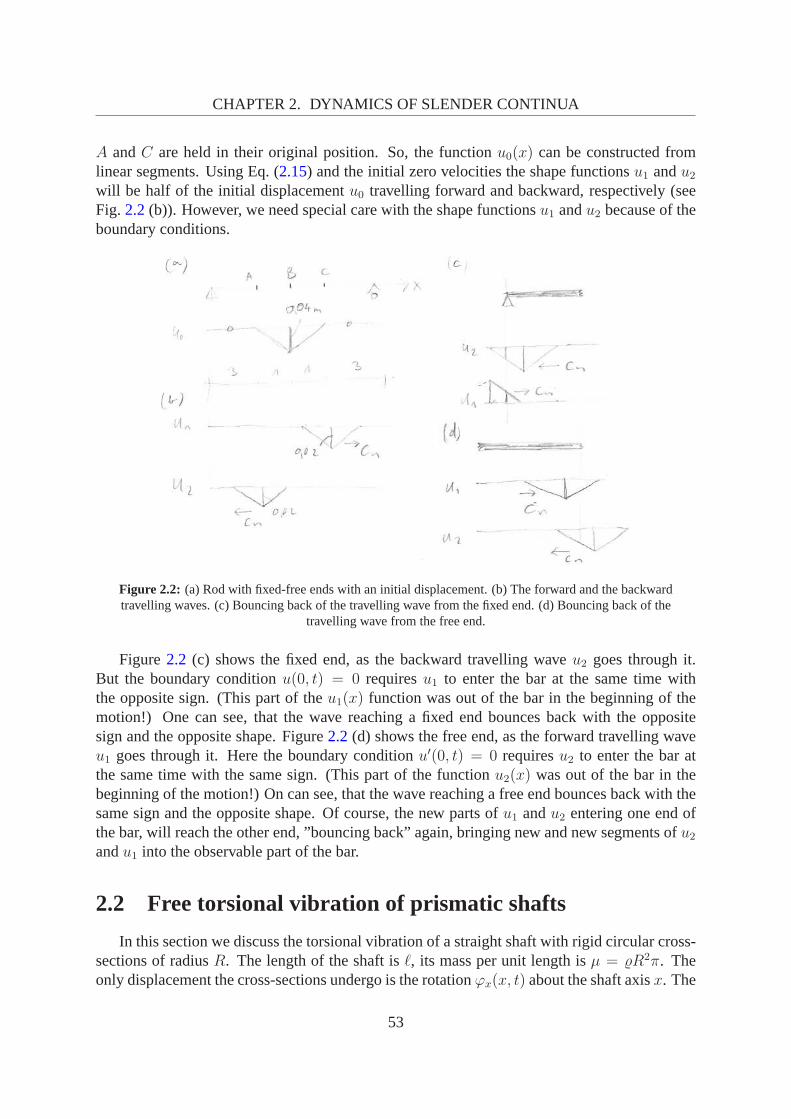
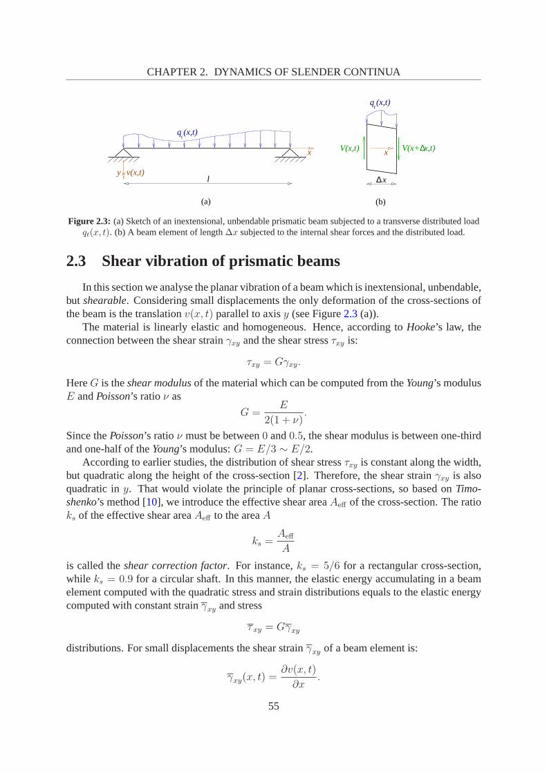
2.1 Sketch of (a) a prismatic bar subjected to a longitudinaldistributed loadqn(x, t) 482.2 Rod with fixed-free ends with an initial displacement and the travelling waves . 532.3 Sketch of an inextensional, unbendable prismatic beam subjected to a trans-

verse, distributed loadqt(x, t) . . . . . . . . . . . . . . . . . . . . . . . . . . . 55

iv

LIST OF FIGURES

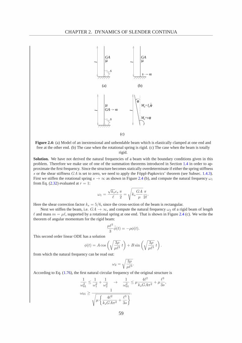
2.4 Model of an inextensional and unbendable beam which is elastically clampedat one end and free at the other end . . . . . . . . . . . . . . . . . . . . . . .. 59

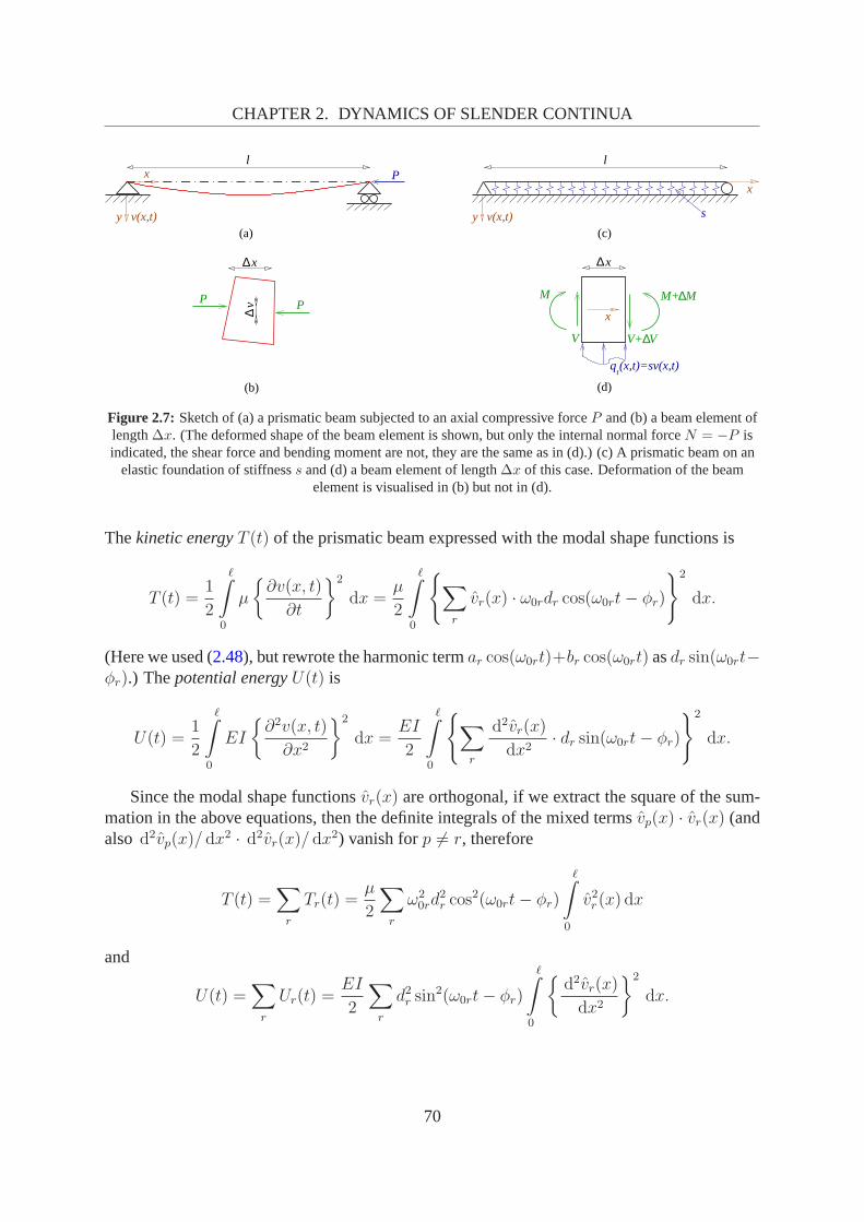
2.5 Sketch of a prismatic beam subjected to a transverse, distributed loadqt(x, t) . 612.6 Common types of supporting modes . . . . . . . . . . . . . . . . . . . . .. . 632.7 Sketch of a prismatic beam subjected to an axial compressive force . . . . . . . 702.8 Prismatic beam subjected to a harmonic exciting forceF sin(ωt) . . . . . . . . 76

3.1 Comparing discrete models of beam structures . . . . . . . . . .. . . . . . . . 833.2 Local and global reference systems . . . . . . . . . . . . . . . . . .. . . . . . 843.3 Model of a frame structure . . . . . . . . . . . . . . . . . . . . . . . . . .. . 853.4 Sketch of the deformed shape of a fixed-fixed beamij due to a unit translation

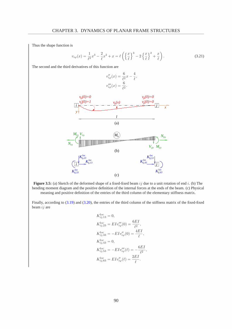
of endi along axisy, and the corresponding bending moment diagram . . . . .873.5 Sketch of the deformed shape of a fixed-fixed beamij due to a unit rotation of

endi, and the corresponding bending moment diagram . . . . . . . . . . .. . 903.6 Elastically supported node . . . . . . . . . . . . . . . . . . . . . . . .. . . . 993.7 Sketch of the deformed shape of beamij due to a harmonic translation of unit

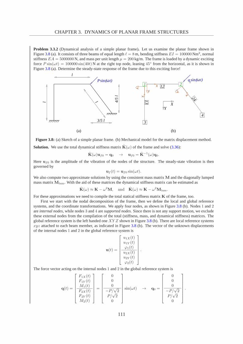
amplitude of endi along axisy, and the corresponding bending moment diagram1053.8 Sketch of a simple planar frame and the mechanical model for the matrix dis-

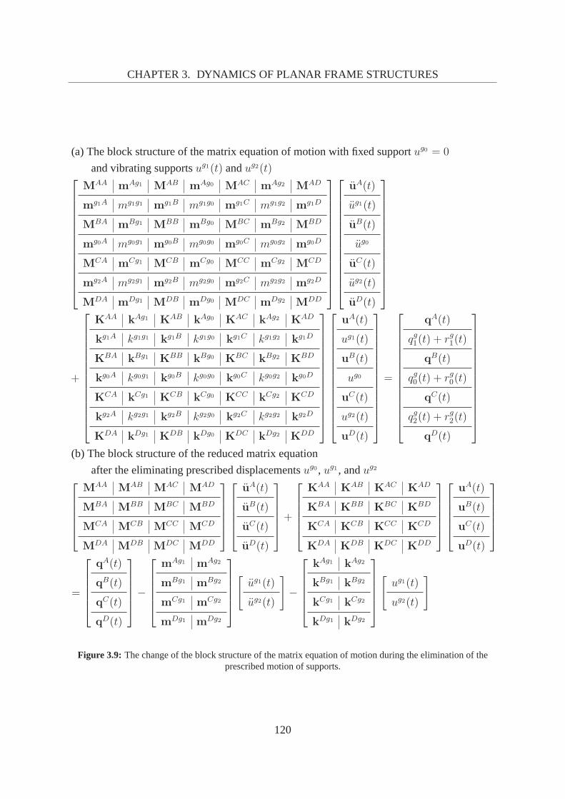
placement method . . . . . . . . . . . . . . . . . . . . . . . . . . . . . . . . .1113.9 The change of the block structure of the matrix equation of motion during the

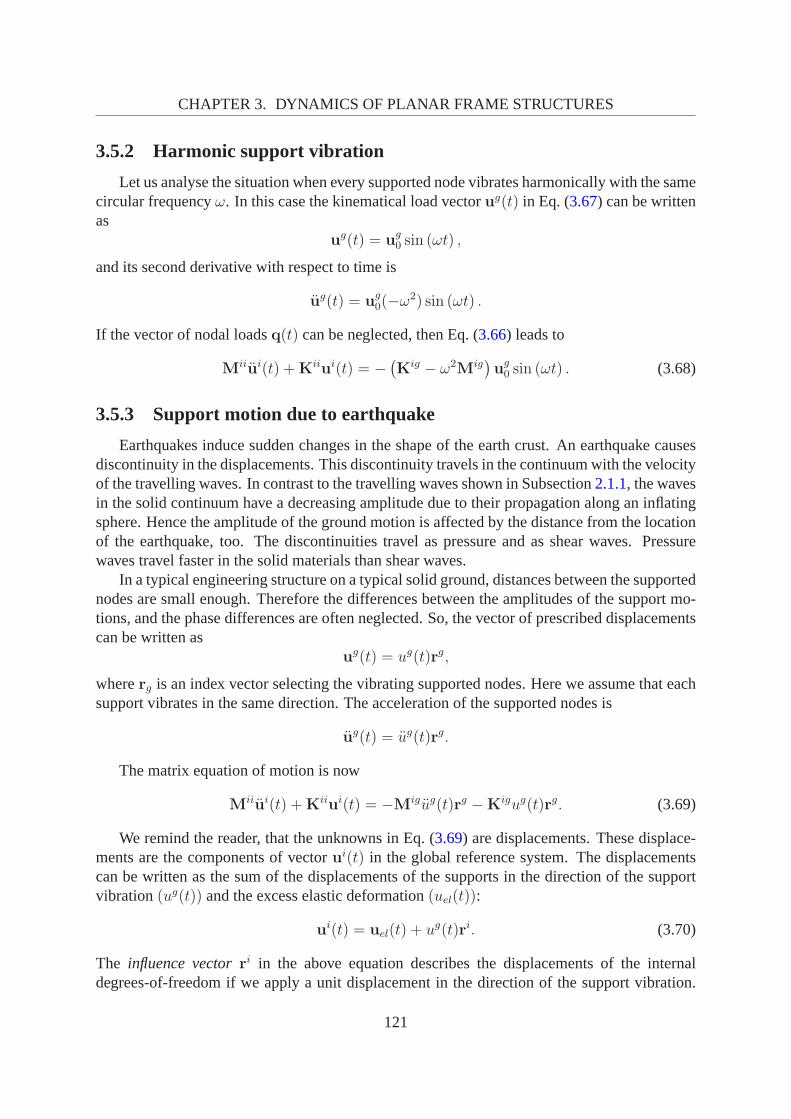
elimination of the prescribed motion of supports. . . . . . . . .. . . . . . . . 1203.10 Sketch of a fixed-fixed beam and the mechanical model for the matrix displace-

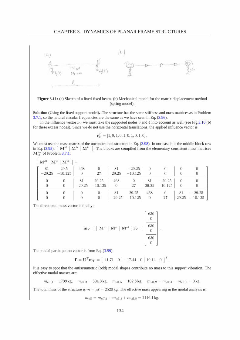
ment method (fixed support model) . . . . . . . . . . . . . . . . . . . . . . .. 1303.11 Sketch of a fixed-fixed beam and the mechanical model for the matrix displace-

ment method (spring model) . . . . . . . . . . . . . . . . . . . . . . . . . . .1343.12 Sketch of the deformed shape of beamij due to a harmonic translation of unit

amplitude of endi along axisy, and the corresponding bending moment diagram1363.13 Demonstration of the moment caused by the normal forceS on a rotated ele-

mentary segment of the beam. . . . . . . . . . . . . . . . . . . . . . . . . . .140

4.1 Sketch of the deformed shape of a damped beam and the bending momentdiagram due to a dynamical vibration of endi along axisy. . . . . . . . . . . . 149

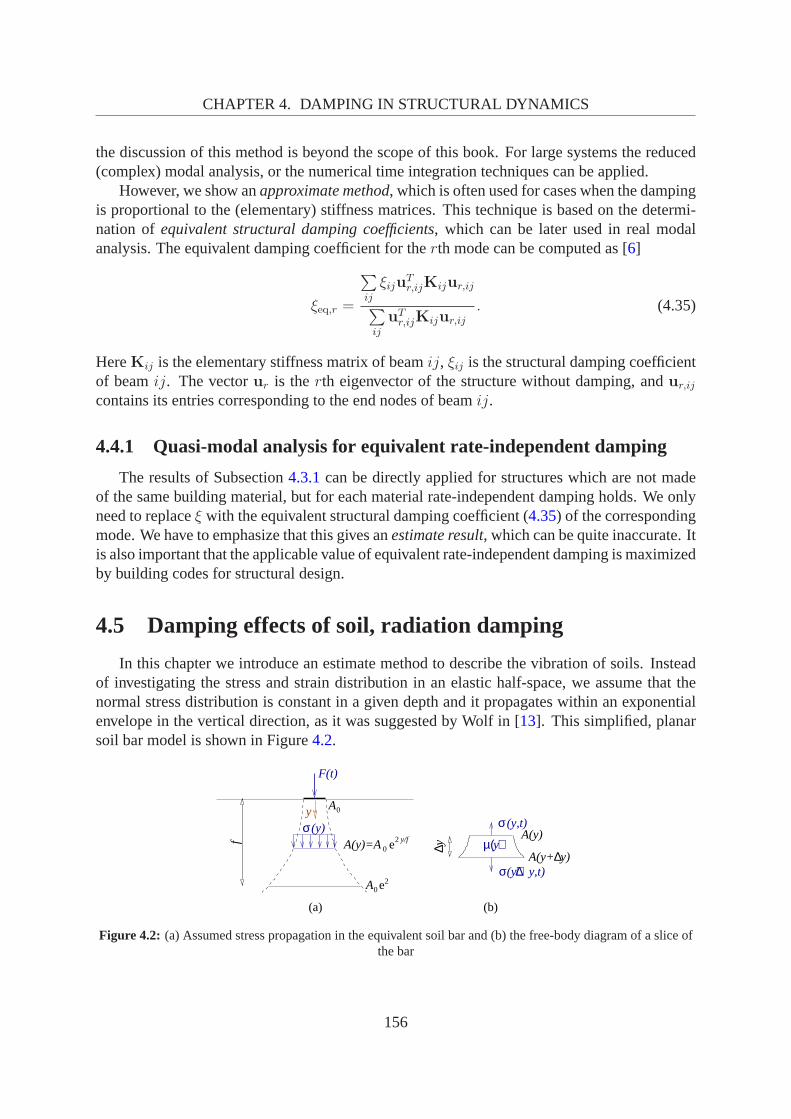
4.2 Assumed stress propagation in the equivalent soil bar . .. . . . . . . . . . . . 156

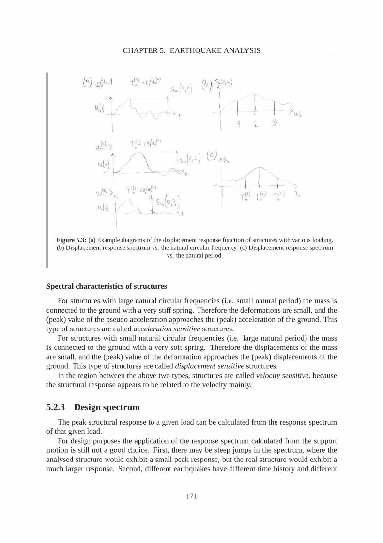
5.1 Solid and surface waves . . . . . . . . . . . . . . . . . . . . . . . . . . . .. . 1675.2 Response functions . . . . . . . . . . . . . . . . . . . . . . . . . . . . . . . .1695.3 Concept of response spectrum . . . . . . . . . . . . . . . . . . . . . . . .. . 1715.4 The functionβ(T0) of the pseudo-acceleration response vs. the natural period. . 1725.5 Force-deformation diagram of the linear elastic-plastic material model and

structure. . . . . . . . . . . . . . . . . . . . . . . . . . . . . . . . . . . . . .1775.6 Typical envelope functions of artificial earthquake records. . . . . . . . . . . .178

A.1 The first four partial sums of the Fourier series for a square wave. Source:Wikimedia Commons . . . . . . . . . . . . . . . . . . . . . . . . . . . . . . .194

v

LIST OF TABLES

List of Tables

1.1 Harmonic forcing of a three-storey structure. Modal loads, coefficients of res-onance, and other parameters . . . . . . . . . . . . . . . . . . . . . . . . . .. 30

3.1 The first few natural circular frequencies of the frame and all the six natural cir-cular frequencies of the approximate models (with the consistent the diagonallylumped mass matrices). The dimension of the frequencies is rad/s. . . . . . . .115

3.2 The first six natural circular frequencies of the frame, the projections of theload vector to the modal shape vectors, and the modal participation factors . . .125

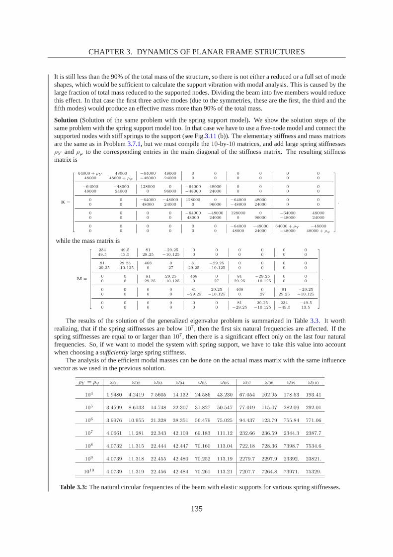
3.3 The natural circular frequencies of the beam with elastic supports for variousspring stiffnesses. . . . . . . . . . . . . . . . . . . . . . . . . . . . . . . . .135

vi

PREFACE

Preface

This lecture notes of the MSc course Structural Dynamics is devoted for the civil engineer-ing students of the Budapest University of Technology and Economics. The objective of thecourse is to introduce the basic concepts of the dynamical analysis of engineering structures.The topics that are covered in this course are equations of motion of single- and multi-degree-of-freedom systems, free and steady-state vibrations, analytical and numerical solution tech-niques, and earthquake loads on structures. Both continuum and discrete mechanical systemsare considered.

In civil engineering practice structures are aimed to be in equilibrium. However, due tocontinuous disturbances (effects of wind, heat, traffic, movement of the foundations, etc.), thestructures undergo vibrations. Some of these motions are slow, allowing us to treat them asa quasi-statickinematic load, and to neglect the inertial effect of the mass of the structure.But some of them happen fast enough to exert a significant dynamical impact on the structure.Many of these cases are still handled as a quasi-static load with a proper dynamical factor,but other cases really require the engineers to accomplish dynamical analysis. The goal of thesemester is to prepare our students for these tasks.

Dynamics play an important role in many fields of structural engineering. Earthquakes, fastmoving trains on bridges, urban traffic generated or machineinduced vibrations, etc. Mod-ern materials enable the fabrication of lighter, more flexible structures, where the effects ofvibrations can be significantly high. Additionally, investment companies desire cost effectivestructures, which also tends the engineers towards more accurate computations, which impliesdynamical analysis, too.

Not only theory is given in this notes, but there are also manyproblems solved. The authorshope that these examples help our students to comprehend allthe introduced concepts. In theseproblems the calculations are done following thecare your unitsapproach. It means that we usea consistent system of units, which does not require us to carry the units during the operations.Every number is substituted in the formulae in a common system of units, in SI (InternationalSystem of Units), hence the results are also obtained in SI.

We offer these notes to our readers under a Creative Commons Attribution-NonCommercial-NoDerivs 3.0 Unported License, in the hope itwill help them understandthe basics of structural dynamics. Please feel free to shareyour thoughts about it with us.

Budapest, 29th August, 2013

vii

CHAPTER 1. DYNAMICS OF SINGLE- AND MULTI-DOF SYSTEMS

Chapter 1

Dynamics of single- andmulti-degree-of-freedom systems

In this chapter first we repeat the basics of vibration of elastic structures. The motion ofcontinuous structures is often approximated by the displacements of some of its points. Inthese models the mass of the structure is concentrated into discrete points. The concentratedmasses are assumed to be rigid bodies, and the elasticity andthe viscoelasticity of the structureis modeled by massless springs and damping elements, respectively. These models are calledmass-spring-dampersystems.

We introduce thedegree-of-freedom(DOF) as the number of independent variables requiredto define the displaced positions of all the masses. If there is only one mass, with one directionof displacement, then we talk about asingle-degree-of-freedom(SDOF) system. If there aremore than one masses, or one mass with more than one directions of displacement, then wehave amulti-degree-of-freedom(MDOF) system. If we try to describe the deformed shape ofa continuous structure with the displacements of all of (infinitely many of) its points, then weuse a continuum approach, where there are infinitely many degrees of freedom.

In Section1.1 we start with the free vibration of SDOF systems, then harmonic forcedvibration of SDOF systems, and support vibration of SDOF systems are discussed. Then SDOFsystems excited by a general force are studied in Section1.2. Section1.3is devoted for the freevibration of MDOF systems. We also present an approximate method capable to solve thegeneralized eigenvalue problem occurring in the analysis of MDOF systems. At the end of thechapter, in Section1.4 we present a few summation theorems useful to approximate the firstnatural frequency of a structure.

1.1 Vibration of single-degree-of-freedom systems

Civil engineering structures are intended in general to be inequilibrium. Despite the com-mon requirements, many of the loading situations result in motion of the structures. The mostsimple motion occurs when we can describe it by one single space variable.

Examples for these type of dynamical systems are horizontalgirders with a significant mass(e.g. a machine, where the mass of the girder can be neglectedwith respect to the mass of the

1


machine) (Figure1.1 (a-b)), frame structures with significant mass on the rooftop (Figure1.1(c)), chimneys and water towers (Figure1.1(d)), etc..

Figure 1.1: Common examples of single-degree-of-freedom structures:(a) fixed girder, (b) hinged-hingedgirder, (c) single frame with mass on rooftop, (d) chimney orwater-tower, and (e) common mechanical model.

The common in the above examples is that any displacement from the equilibrium stateresults a force pulling the DOF back to the initial state. Thesimplest mechanical model of thisbehaviour is the material particle (lumped mass) connectedby a linear spring to a rigid wall(Figure1.1(e)).

1.1.1 Derivation of the equation of motion

If we analyse the motion of a structure caused by a small disturbance, then we can see that inthe absence of external forcing the amplitude of the vibration around the original state decreaseswith the time. This is caused by internal friction in the material and at the connections. Effectof external dampers can be considered as well. The mathematically easiest way to deal withdamping is the viscous damping. (In this case the damping force is proportional to the velocity.)The mechanical model of the viscous damping is adashpot. Figure1.2 (a) shows a damped,elastically supported system with a dashpot of damping coefficient c, a linear elastic springof stiffnessk, and a time dependent exciting forceF (t). Our goal is in general one of thefollowings:

• to find the displacement function as a function of time

• to find the elongation of the spring as a function of time

• to find the force in the spring or in the dashpot as a function oftime

• to find the possible maxima of the above functions

2


Figure 1.2: (a) A mass-spring-damper model: a lumped massm is connected to a support through a masslesslinear springk and a massless viscous damperc. The mass excited by the time dependent forceF (t) undergoing

a single-degree-of-freedom vibration. (b) Free body diagram of the mass-spring-damper model.

The free body diagram (FBD) of the massm can be seen in Figure1.2(b). Newton’s secondlaw of motion can be written for the body:

F (t)− fs(t)− fd(t) = ma(t), (1.1)

whereF (t) is the external force,fs(t) is the elastic force from the massless spring,fd(t) isthe damping force from the massless dashpot,m is the mass anda(t) is the acceleration. As-suming a linear springfs(t) = ku(t), wherek is the spring stiffness, andu(t) is the elon-gation of the spring. Assuming a viscous dampingfd(t) = cu(t), wherec is the dampingcoefficient, andu(t) is the derivative of the elongationu(t) with respect to time (i.e. it is theelongation-velocity). (The dot over a variable denotes differentiation with respect to time.) Theaccelerationa(t) is the second derivative of the displacement of the body withrespect to time:a(t) = x(t). So the equation of motion is:

F (t)− ku(t)− cu(t) = mx(t). (1.2)

(Note: in many textbook authors write a so called kinetic equilibrium equation using the principleof d’Alembertwith an inertial forcefI = −ma(t). Then, Eq. (1.1) would have the form:F (t)−fs(t)−fd(t) + fI(t) = 0. In formal calculation it leads to the same result, but during calculations by handthe correct interpretation of the minus sign in the definition offI requires a deep understanding of theconcept, at which level writing the classic formula makes no problem. Because of that we will avoidwriting kinetic equilibrium equations. )

In most cases we are interested in the internal deformationsand the corresponding internalforces of the structures. These are represented in this model by the elongation of the spring,so we have to write the displacement of the body as a function of elongation. If the support isfixed, then these two values are equal (x(t) = u(t)) and the same applies to their derivatives(x(t) = u(t)). Substituting these into Eq. (1.2) we get:

mu(t) + cu(t) + ku(t) = F (t) . (1.3)

This non-homogeneous, linear, second order ordinary differential equation of constant co-efficients describes the motion of the forced vibration of the damped SDOF-system.

3


For the solution of the differential equation (1.3) we introduce its complementary differen-tial equation:

mu(t) + cu(t) + ku(t) = 0. (1.4)

which is a homogeneous differential equation. Thecomplete solutionof Eq. (1.3) can be writtenin the form:

u(t) = u0(t) + uf (t),

whereu0(t) is the solution of the complementary equation (the index 0 refers to the 0 righthand side of the homogeneous equation), whileuf (t) is a particular solution of the original,nonhomogeneous equation (the indexf refers to the forcing).

If initial conditions are given (e.g. the displacement and the velocity at a given time), thenthey must be fulfilled for the sum ofu0(t) anduf (t) with the free parameters occurring inu0(t).

1.1.2 General solution of the homogeneous ODE

Eq. (1.4) describes the free vibration of the mechanical system. Since it is a linear, homo-geneous ODE with constant coefficients, the solution can be obtained with an ansatz functionu(t) = eλt, which is substituted back in Eq. (1.4) alongside with is derivatives. The result isthe quadratic polynomial equation

mλ2 + cλ+ k = 0. (1.5)

The roots of the above equation are:

λ1,2 =−c±

√c2 − 4mk

2m. (1.6)

These roots might be either real or complex valued, depending on the ratio of the systemparameters.

• If c ≥ 2√km, the discriminant in Eq. (1.6) is non-negative, thus bothλ1,2 are negative

real numbers, and the solution of Eq. (1.4) is the sum of two exponential function asymp-totically approaching zero. (Figure1.3 (a) shows some typical graphs of this vibration.)We call this damping as heavy damping, the system is an overdamped system. The limitvalue2

√km is the critical dampingccr.

• If c < 2√km (or c < ccr), the discriminant is negative, the solution of Eq. (1.5) is a

conjugate pair of complex numbers. UsingEuler’s formula (e ix = cos x + i sin x) thesolution of Eq. (1.4) can be rewritten in the form:

u0(t) = e−ξω0t (A cos(ω∗0t) + B sin(ω∗

0t)) , (1.7)

whereξ =

c

2√km

=c

ccr

is therelative dampingcoefficient

ω∗0 = ω0

√1− ξ2

4


is thenatural circular frequencyof the (under)damped system,

ω0 =√k/m

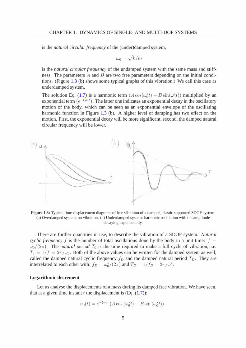
is thenatural circular frequencyof the undamped system with the same mass and stiff-ness. The parametersA andB are two free parameters depending on the initial condi-tions. (Figure1.3 (b) shows some typical graphs of this vibration.) We call this case asunderdamped system.

The solution Eq. (1.7) is a harmonic term(A cos(ω∗0t) +B sin(ω∗

0t)) multiplied by anexponential term

(e−ξω0t

). The latter one indicates an exponential decay in the oscillatory

motion of the body, which can be seen as an exponential envelope of the oscillatingharmonic function in Figure1.3 (b). A higher level of damping has two effect on themotion. First, the exponential decay will be more significant, second, the damped naturalcircular frequency will be lower.

Figure 1.3: Typical time-displacement diagrams of free vibration of a damped, elastic supported SDOF system.(a) Overdamped system, no vibration. (b) Underdamped system: harmonic oscillation with the amplitude

decaying exponentially.

There are further quantities in use, to describe the vibration of a SDOF system.Naturalcyclic frequencyf is the number of total oscillations done by the body in a unit time: f =ω0/(2π). The natural periodT0 is the time required to make a full cycle of vibration, i.e.T0 = 1/f = 2π/ω0. Both of the above values can be written for the damped system as well,called the damped natural cyclic frequencyfD and the damped natural periodTD. They areinterrelated to each other with:fD = ω∗

0/(2π) andTD = 1/fD = 2π/ω∗0.

Logarithmic decrement

Let us analyse the displacements of a mass during its damped free vibration. We have seen,that at a given time instantt the displacement is (Eq. (1.7)):

u0(t) = e−ξω0t (A cos (ω∗0t) + B sin (ω∗

0t)) .

5


Using the previously introduced damped natural periodTD, we can write the displacement aftera whole period of motion as well:

u0(t+ TD) = e−ξω0(t+TD) (A cos (ω∗0(t+ TD)) + B sin (ω∗

0(t+ TD))) .

The ratio of the displacements can be written as:

u0(t)

u0(t+ TD)=

e−ξω0t (A cos (ω∗0t) +B (sinω∗

0t))

e−ξω0(t+TD) (A cos (ω∗0(t+ TD)) + B sin (ω∗

0(t+ TD))).

SinceTD is the damped period of the motion, the harmonic terms in bothtime instants have thesame value, so we can simplify the above formula as

u0(t)

u0(t+ TD)= eξω0TD = e

(

2ξπ/√

1−ξ2)

. (1.8)

This ratio is constant, and depends only on the dampingξ. Since we did not have any constrainton t, Eq. (1.8) holds for any two displacements measured in a time distanceTD. In practice,the natural logarithm of Eq. (1.8) is used for the measurement of damping

ϑ = lnu0(t)

u0(t+ TD)= 2ξπ/

√1− ξ2.

Hereϑ is called thelogarithmic decrementwhich is a system property. In typical engineeringstructuresξ ≪ 1, so the

√1− ξ2 ≈ 1 approximation can be used:

ϑ = lnu0(t)

u0(t+ TD)≈ 2ξπ. (1.9)

Free vibration of undamped systems

The vibration of undamped systems can be derived in a similarway as we did it for thedamped system, or we can analyse our damped results in the limit c → 0. According toEq. (1.3) the differential equation of motion can be written as:

mu(t) + ku(t) = F (t).

The complementary equation describes the undamped free vibration:

mu(t) + ku(t) = 0.

The solution of the free vibration is directly obtained fromEq. (1.7) at c = 0 (andξ = 0):

u0(t) = A cos(ω0t) + B sin(ω0t).

Hereω0 =√k/m is thenatural circular frequencyof the undamped system. The parameters

A andB can be calculated from the initial conditions. The purely harmonic motion can berewritten into the form:

u0(t) = C sin (ω0t+ ϕ) ,

with the amplitude of the motionC =√A2 +B2 and the phase angleϕ = arctan A

B.

6


1.1.3 Particular solution of the non-homogeneous ODE with harmonicforcing

A simple example for a harmonic excitation force is a rigid body (e.g. a machine) rotatingwith a constant angular velocityω around an axis which is not going through its center ofgravity (COG). The distance between the axis and the center ofgravity is called the eccentricityand denoted byrC .) The COG of the body undergoes a planar motion on a circular path with anangular velocityω. From kinematics of rigid bodies the acceleration of the COG equalsan =mω2rC , its direction varies with the motion, its component parallel with an arbitrary chosen, butfixed direction can be written as a harmonic function of time,and the same applies for the netforce acting on the rigid body. The opposite of this force acts on the axis of rotation, resultingin a harmonic excitation force on the load bearing structure. (The orthogonal component ofthe force should be taken into account as well, but the vibration can be prevented by structuralconstraints, or by applying two well-tuned body rotating inthe opposite direction.)

Without loss of generality (for harmonic functions one can translate the time scale to haveany other harmonic function with the same frequency and amplitude), we will write the har-monic excitation force in the form:

F (t) = F0 sin (ωt) .

HereF0 is the amplitude of the force, andω is the circular frequency of the forcing. Substitutingthis forcing in the right hand side of (1.3) yields:

mu(t) + cu(t) + ku(t) = F0 sin (ωt) . (1.10)

To solve Eq. (1.10) we assume that the particular solution is of the form:

uf (t) = uf0 sin (ωt− ϕ) ,

i.e. it is a harmonic function with the same frequency as the forcing, but with a phase shift ofϕ. We substitute our ansatz into Eq. (1.10):

−mω2uf0 sin (ωt− ϕ) + cωuf0 cos (ωt− ϕ) + kuf0 sin (ωt− ϕ) = F0 sin (ωt) .

We apply trigonometrical identities for the sums in the sineand cosine functions:

−mω2uf0 sin (ωt) cos(−ϕ)−mω2uf0 cos (ωt) sin(−ϕ) + cωuf0 cos (ωt) cos(−ϕ)− cωuf0 sin (ωt) sin(−ϕ) + kuf0 sin (ωt) cos(−ϕ) + kuf0 cos (ωt) sin(−ϕ) = F0 sin (ωt) .

Now we separate the sinusodial and cosinusoidal parts:

uf0 cos (ωt)(mω2 sinϕ+ cω cosϕ− k sinϕ

)

+ uf0 sin (ωt)(−mω2 cosϕ+ cω sinϕ+ k cosϕ

)= F0 sin (ωt) .

This equation must hold for any timet.

7


• Whensin (ωt) = 0, thencos (ωt) 6= 0, so

mω2 sinϕ+ cω cosϕ− k sinϕ = 0

must hold, which is true, when

cotϕ =k −mω2

cω=m

c

ω20 − ω2

ω, (1.11)

with 0 ≤ ϕ ≤ π. (See Figure1.4 (a) for the dependence of phase angle on the ratio ofthe forcing and natural frequency.)

• Whencos (ωt) = 0, thensin (ωt) 6= 0, so

uf0(−mω2 cosϕ+ cω sinϕ+ k cosϕ

)= F0

must hold.

We use the identitiescosϕ = cotϕ/√

1 + cot2 ϕ andsinϕ = 1/√

1 + cot2 ϕ to get

uf0−mω2 cotϕ+ cω + k cotϕ√

1 + cot2 ϕ= F0

and solve the above equation foruf0 using Eq. (1.11):

uf0 = F0

√1 + (k−mω2)2

c2ω2

(k −mω2) k−mω2

cω+ cω

.

Multiplying both the nominator and the denominator withcω leads to

uf0 = F01√

(k −mω2)2 + c2ω2

=F0

k

1√(1− m

kω2)2

+ c2

k2ω2

Using the natural circular frequency and the fraction of critical damping coefficient (ω0 =√k/m, ξ = c/(2

√km)) the solution foruf0 is

uf0 =F0

k

1√(1− ω2

ω20

)2+ 4ξ2 ω

2

ω20

. (1.12)

From the above results the particular solution of the differential equation (1.10) of the harmon-ically forced vibration is:

uf (t) =F0

k

1√(1− ω2

ω20

)2+ 4ξ2 ω

2

ω20

sin

ωt− arccot

1− ω2

ω20

2ξ ωω0

. (1.13)

8


The complete solution of Eq. (1.10) is the sum of Eq. (1.13) and (1.7):

u(t) =F0

k

1√(1− ω2

ω20

)2+ 4ξ2 ω

2

ω20

sin

ωt− arccot

1− ω2

ω20

2ξ ωω0

+ e−ξω0t (A cos (ω∗0t) +B sin (ω∗

0t)) .

(1.14)

The second part of Eq. (1.14) becomes very small after a sufficiently long time for any smalldamping. That part is called thetransient vibration. The first part, which is equivalent tothe particular solution Eq. (1.13), is called thesteady-statesolution of the problem. Sincethe transient vibration decays exponentially with time, ona long time scale the steady-statevibration determines the dynamics. Usually we are not interested in the phase of the motion,but in the amplitude of the vibrationuf0, given by Eq. (1.12). In that formula the quotientF0/kcan be regarded as thestatic displacementunder a static forceF0 (which is the amplitude ofthe harmonic forcing). We will refer to it as the static displacementust. The static displacementust = F0/k is multiplied by a coefficient in Eq. (1.12), which depends on the damping andon the ratio of the circular frequency of the forcing to the natural circular frequency of thesystem. We call this quantity as theresponse factor, and denote it byµ. Figure1.4 (b) showsthe dependence of the response factor on the ratio of frequencies.

Figure 1.4: Responses of a damped SDOF system to a harmonic excitation: (a) phase angleϕ as a function of theforcing frequencyω, (b) response factorµ as a function of the ratio of the forcing and natural frequenciesω/ω0.

In short, the amplitude of the steady-state vibration can bewritten as:

uf0 = ustµ ,

where

ust =F0

k(1.15)

and

µ =1√(

1− ω2

ω20

)2+ 4ξ2 ω

2

ω20

. (1.16)

9


Now we further analyse the response factor functionµ. For smallω/ω0 it is small, but big-ger than1. As ω/ω0 approaches1 it reaches a maximum. One can derive, that the maximumoccurs atω/ω0 =

√1− 2ξ2, but in the practical range of dampingξ of engineering structures,

the difference can be neglected, so in general we can say, that the maximal amplitude is ap-proximately atω = ω0 with the magnitudeµmax

∼= 1/(2ξ). The state whenµ is maximal iscalled theresonance. For the case, whenω > ω0, the response factor decreases asymptoticallyto zero.

The spring force from the steady-state part of the motion canbe calculated from the elon-gation of the spring:

FS0 = kustµ = F0µ,

i.e. the amplitude of the excitation force multiplied by theresponse factor, thus for fast exci-tation with largeω or flexible structure with lowω0 the spring force will be small due to thedecaying response factorµ. But if we are looking for the force transmitted to the base, wealsohave to take into account the forcefD in the damping element, which may result higher baseforces.

Effect of zero damping on the phase angle and response factor

The vibration of undamped systems can be derived in a similarway as for the dampedsystem, or we can analyse our damped results in the limitc → 0. In the latter case we canconclude, that the particular solution of the non-homogeneous differential equation (1.10) isa harmonic vibration. The amplitude of the vibration can be calculated from Eq. (1.12) withξ → 0:

uf0 =F0

k

1√(1− ω2

ω20

)2 =F0

k

1

|1− ω2

ω20

|.

It is the product of the static displacement and the (undamped) response factor (see Fig.1.4(b)). In contrast to the damped case, this response factor has an infinite maximum in the stateof resonance (ω = ω0).

For the phase angleϕ we can conclude from Eq. (1.11) that it is zero whenω < ω0, andit is π whenω > ω0 (see Fig.1.4 (a)). In the first case the mass movesin-the-phasewith theexcitation force, in the second case the mass movesout-of-the-phasewith the excitation force.At the resonance stateω = ω0 the phase angle isϕ = π/2.

Ideal damping

Analysis of the damped response factor Eq. (1.16)) and its derivative with respect toωω0

results that an increasing damping coefficientξ decreases the location and the value of themaximum ofµ (see Fig.1.4(b)). If ξ reaches1/

√2, then the location of the maximum reaches

ω = 0, and the value of the maximum reaches1. Further increase of the damping decreases theresponse factor, but the maximum will be always1 atω = 0. This damping valueξid = 1/

√2

(or cid =√2km) is called theideal damping.

10


1.1.4 Support vibration of SDOF systems

In many cases the support of the structure is not in rest. During an earthquake or because ofthe noise of traffic the base (which was assumed until now to bein rest) might move, makingthe structure to vibrate.

In this subsection we will show how to handle the support motion for undamped systems.The steps of the solution would be the same for a damped systemas well.

In the case of support vibration we have to modify our mechanical model shown in Fig.1.2(a) such that we set the damping to zero (c = 0) and apply a support motionug(t) (where theindexg refers to the ground motion). Figure1.5(a) shows this model.

If we draw the free body diagram, there is only one force acting on the body from the spring,so we can write Newton’s second law of motion based on Figure1.5(b) as

−fS(t) = ma(t),

or by substituting the spring forcefS(t) = ku(t) and the accelerationa(t) = u(t) as

− ku(t) = mx(t). (1.17)

Figure 1.5: Support vibration of an undamped system (a) mechanical model, (b) free body diagram

The elongation of the spring is now

u(t) = x(t)− ug(t), (1.18)

and the second derivative of the Eq. (1.18) results:

u(t) = x(t)− ug(t). (1.19)

One can follow two different approaches.

• Substitution ofu(t) from Eq. (1.18) in Eq. (1.17) leads to

−kx(t) + kug(t) = mx(t),

which is a differential equation for the displacementx(t) of the body. If we write it in acanonical form

mx(t) + kx(t) = kug(t) (1.20)

one can see, that it is a simple forced vibration.

11


• Substitution ofx(t) from Eq. (1.19) in Eq. (1.17) implies

−ku(t) = mu(t) +mug(t),

which is a differential equation for the elongationu(t) of the spring. If we write it in acanonical form

mu(t) + ku(t) = −mug(t), (1.21)

we obtain a simple forced vibration again.

In the next subsections we will show the solutions of the derived differential equations fora harmonic support vibration, i.e.ug(t) = ug0 sin(ωt).

Steady-state solution of the elongation of the spring due toa harmonic support motion

To find the solution of Eq. (1.21) we have to substitute the second derivative ofug(t)

ug(t) = −ω2ug0 sin(ωt)

into Eq. (1.21):mu(t) + ku(t) = mω2ug0 sin(ωt).

This is the same equation as Eq. (1.10) with c = 0 andF0 = mω2ug0. Therefore, the amplitudeof the steady-state solution will be (see Eq. (1.12)):

uf0 =mω2ug0

k

1√(1− ω2

ω20

)2 = ug0ω2

ω20

1

|1− ω2

ω20

|.

The amplitude of the elongationu(t) will be the amplitude of the support vibration multipliedby a response factor and by the square of the ratio of the forcing and natural frequencies. Thespring forcefS(t) is related to the elongationu(t) of the spring so its amplitude will be:

fmaxS = kug0

ω2

ω20

1

|1− ω2

ω20

|= f st

S

ω2

ω20

1

|1− ω2

ω20

|.

Heref stS is the static force, which would cause an elongationug0 in the spring.

Figure1.6shows the product of two multipliers(ω2/ω20 and1/|1− ω2/ω2

0|) as the functionof the ratio of the forcing and natural frequencies.

Steady-state solution of the displacementx(t) for harmonic support vibration

To find the solution of Eq. (1.20) we have to substituteug(t) into Eq. (1.20):

mx(t) + kx(t) = kug0 sin(ωt).

This is the same equation as Eq. (1.10) with c = 0 andF0 = kug0. Thus, the amplitude of thesteady-state solution is (see Eq. (1.12)):

xf0 =kug0k

1√(1− ω2

ω20

)2 = ug01

|1− ω2

ω20

|.

12


Figure 1.6: Response factor of the elongation of the spring as a functionof the ratio of the forcing and naturalfrequencies due to a harmonic support vibration

1.2 General forcing of SDOF systems

1.2.1 Duhamel’s integral

Static (or quasi-static) loads and harmonic forcing represent only a small segment of thepossible loads acting on a structure. Although many of the time-dependent loads can be treatedas a quasi-static, or a sum of harmonic loads, there are important excitation forms (impact,support vibration due to earthquakes, etc.) where the transient behavior of the structure mustbe analyzed. For this type of problem the equation of motion Eq. (1.3)

mu(t) + cu(t) + ku(t) = q(t) (1.22)

contains an arbitrary functionq(t) on the right hand side (see Figure1.7 (a)). We are lookingfor the particular solutionuf (t) of Eq. (1.22) for the t > 0 interval, with the assumption thatwe know the initial displacement and velocity in the time instant t = 0. We denote these twoinitial conditions withuf (0) = u0 and uf (0) = v0. We remind the reader that the solutionof a non-homogeneous differential equation always consists of the solution of the complemen-tary equation (the free vibrational part) with free parameters, and a particular solution of thenon-homogeneous equation. The free vibration follows the classical scheme we presented inSubsection1.1.2.

We assumed linear response of the elastic and damping elements (k andc are constants),so the differential equation is linear, and the rule of superposition holds. If the excitation forcecan be written in the formq(t) =

∑Ni=1 qi(t), then the particular solution can be expressed as

uf (t) =∑N

i=1 ufi(t), where eachufi is a particular solution of the differential equation

mu(t) + cu(t) + ku(t) = qi(t).

Let us choose a sufficiently small time interval∆τ at the time instantt = τ , as shown inFigure1.7 (a), and let us examine the effect of the forceq(τ) during the interval∆τ on thedisplacementuf (t). This specific part of the forcing is shown in Figure1.7 (b). We denote

13


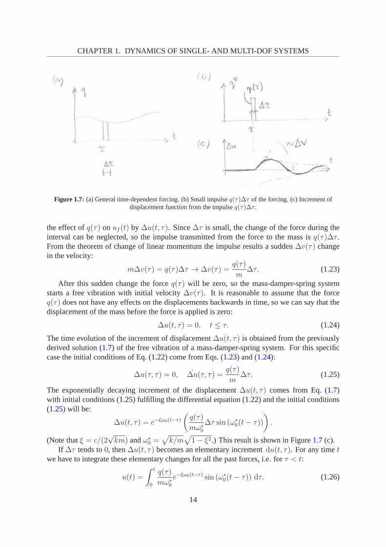
Figure 1.7: (a) General time-dependent forcing. (b) Small impulseq(τ)∆τ of the forcing. (c) Increment ofdisplacement function from the impulseq(τ)∆τ .

the effect ofq(τ) on uf (t) by ∆u(t, τ). Since∆τ is small, the change of the force during theinterval can be neglected, so the impulse transmitted from the force to the mass isq(τ)∆τ .From the theorem of change of linear momentum the impulse results a sudden∆v(τ) changein the velocity:

m∆v(τ) = q(τ)∆τ → ∆v(τ) =q(τ)

m∆τ. (1.23)

After this sudden change the forceq(τ) will be zero, so the mass-damper-spring systemstarts a free vibration with initial velocity∆v(τ). It is reasonable to assume that the forceq(τ) does not have any effects on the displacements backwards in time, so we can say that thedisplacement of the mass before the force is applied is zero:

∆u(t, τ) = 0, t ≤ τ. (1.24)

The time evolution of the increment of displacement∆u(t, τ) is obtained from the previouslyderived solution (1.7) of the free vibration of a mass-damper-spring system. For this specificcase the initial conditions of Eq. (1.22) come from Eqs. (1.23) and (1.24):

∆u(τ, τ) = 0, ∆u(τ, τ) =q(τ)

m∆τ. (1.25)

The exponentially decaying increment of the displacement∆u(t, τ) comes from Eq. (1.7)with initial conditions (1.25) fulfilling the differential equation (1.22) and the initial conditions(1.25) will be:

∆u(t, τ) = e−ξω0(t−τ)

(q(τ)

mω∗0

∆τ sin (ω∗0(t− τ))

).

(Note thatξ = c/(2√km) andω∗

0 =√k/m

√1− ξ2.) This result is shown in Figure1.7(c).

If ∆τ tends to0, then∆u(t, τ) becomes an elementary incrementdu(t, τ). For any timetwe have to integrate these elementary changes for all the past forces, i.e. forτ < t:

u(t) =

∫ t

0

q(τ)

mω∗0

e−ξω0(t−τ) sin (ω∗0(t− τ)) dτ. (1.26)

14


The above formula is theDuhamel’s integral.

1.2.2 Numerical solution of the differential equation

For many types of excitation forcesDuhamel’s integral (1.26) can be computed only nu-merically. Instead of numerical integration of the formula(1.26) the step-by-step calculation ofthe displacements and velocities directly from the differential equation (1.22) is possible.

In the numerical calculations it is a quite usual step to reformulate the second order dif-ferential equation into two, first order equations. For that, first we introduce a new variablefunction, the velocity:

v(t) =du(t)

dt,

and put it and its derivative with respect to time in the original, second order differential equa-tion (1.22). The resulting system of first order differential equations is:

du(t)

dt= v(t),

dv(t)

dt= − c

mv(t)− k

mu(t) +

q(t)

m,

(1.27)

with initial conditionsu(t0) = u0 andv(t0) = v0.

Cauchy-Euler method

Let us assume, that we know the displacement and the velocityat a given time instantti,and we want to calculate them at the time instantti+1. (Let the difference betweenti+1 andtibe a chosen constant∆t = ti+1 − ti.) We denote the displacement and the velocity atti by uiandvi. From Eq. (1.27) we can calculate the differences∆ui/∆t and∆vi/∆t:

∆ui∆t

=ui+1 − ui

∆t= vi,

∆vi∆t

=vi+1 − vi

∆t=

(− c

mvi −

k

mui +

q(ti)

m

).

The estimated values of both variablesui+1 andvi+1, are

ui+1 = ui + vi∆t,

vi+1 = vi +

(− c

mvi −

k

mui +

q(ti)

m

)∆t.

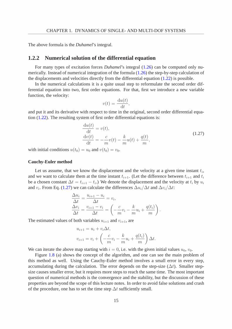
We can iterate the above map starting withi = 0, i.e. with the given initial valuesu0, v0.Figure1.8 (a) shows the concept of the algorithm, and one can see the main problem of

this method as well. Using the Cauchy-Euler method involves asmall error in every step,accumulating during the calculation. The error depends on the step-size (∆t). Smaller step-size causes smaller error, but it requires more steps to reach the same time. The most importantquestion of numerical methods is the convergence and the stability, but the discussion of theseproperties are beyond the scope of this lecture notes. In order to avoid false solutions and crashof the procedure, one has to set the time step∆t sufficiently small.

15


Figure 1.8: Explanation of (a) the Cauchy-Euler method and (b) the second order Runge-Kutta method. Thecontinuous is the exact solution, the arrows represent tangents and increments.

Higher order methods

The key idea behind the higher order methods is to use a betterapproximation for theincrements∆ui, ∆vi, than we had from the tangents calculated at the end-point ofstep i.It seems to be reasonable, that we rather calculate the tangent somewhere along the currentsegment (based on one, or more points). These methods are called theRunge-Kuttamethods.In the second order Runge-Kutta method we calculate the tangent at the middle of the currentsegment. So, we go forward with a half step-size, calculate the tangents there, and use thosevalues to make the actual step-size. It means, that we have tocalculate the derivatives twice asmuch, but we get a higher precision. The algorithm is of the following steps. First we computethe differences just as before:

∆u0i∆t

=ui+1 − ui

∆t= vi,

∆v0i∆t

=vi+1 − vi

∆t=

(− c

mvi −

k

mui +

q(ti)

m

).

Next we step forward with a half step-size:

u1/2i = ui +∆u0i /2,

v1/2i = vi +∆v0i /2.

Then we compute the differences at the mid-point (this will be the direction of the actual step):

ui+1 − ui∆t

= v1/2i ,

vi+1 − vi∆t

=

(− c

mv1/2i − k

mu1/2i +

q(ti +∆t/2)

m

).

Finally, the map of the iteration is

ui+1 = ui +∆ui = ui + v1/2i ∆t,

vi+1 = vi +∆vi = vi +

(− c

mv1/2i − k

mu1/2i +

q(ti +∆t/2)

m

)∆t.

16


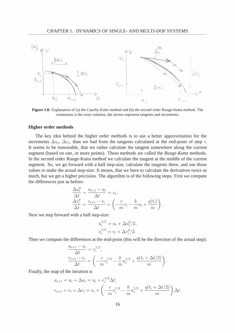
Figure 1.9: Explanation of the finite difference approximation of velocity and acceleration using secant lines

Central difference method

Let us assume, that we know the displacement and the velocityat the given time instancesti−1 andti, and we want to calculate them at the time instantti+1. (Let the difference betweentwo time instants be constant:∆t = ti+1 − ti = ti − ti−1.) We denote the displacement and thevelocity atti by ui andvi, at ti−1 by ui−1 andvi−1, respectively.

We can write the approximation for the velocity (see Figure1.9):

vi = ui ∼=ui+1 − ui−1

2∆t, (1.28)

while the approximation of the acceleration is:

ai = ui ∼=ui+0.5 − ui−0.5

∆t∼= (ui+1 − ui)− (ui − ui−1)

∆t2=ui+1 − 2ui + ui−1

∆t2. (1.29)

The equation of motion is (1.22):

mui + cui + kui = q(ti) = qi.

Let us substitute the velocity (Eq. (1.28)) and the acceleration (Eq. (1.29)) into the above equa-tion:

mui+1 − 2ui + ui−1

∆t2+ c

ui+1 − ui−1

2∆t+ kui = qi. (1.30)

One can solve Eq. (1.30) for ui+1:

ui+1 =

qi + ui

(2m

∆t2− k

)+ ui−1

( c

2∆t− m

∆t2

)

m

∆t2+

c

2∆t

. (1.31)

Eq. (1.31) is the map of the iteration containing only the displacements of the previous twosteps (but no velocities). Therefore, not only the displacementu0 in the initial time instant, butalso the displacementu−1 is needed to start the iteration. This latter condition can be computedfrom u0 andv0 as

u−1 = u0 − v0∆t.

17


1.3 Vibration of multi-degree-of-freedom systems

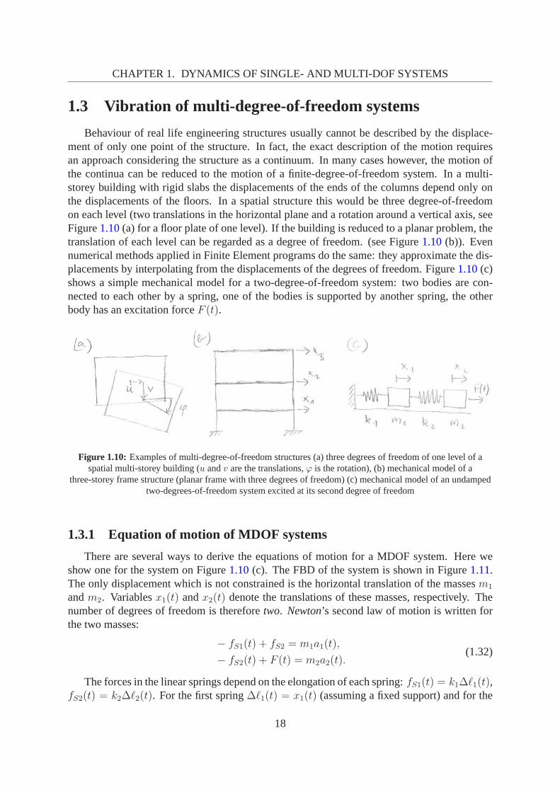
Behaviour of real life engineering structures usually cannot be described by the displace-ment of only one point of the structure. In fact, the exact description of the motion requiresan approach considering the structure as a continuum. In many cases however, the motion ofthe continua can be reduced to the motion of a finite-degree-of-freedom system. In a multi-storey building with rigid slabs the displacements of the ends of the columns depend only onthe displacements of the floors. In a spatial structure this would be three degree-of-freedomon each level (two translations in the horizontal plane and arotation around a vertical axis, seeFigure1.10(a) for a floor plate of one level). If the building is reduced to a planar problem, thetranslation of each level can be regarded as a degree of freedom. (see Figure1.10(b)). Evennumerical methods applied in Finite Element programs do thesame: they approximate the dis-placements by interpolating from the displacements of the degrees of freedom. Figure1.10(c)shows a simple mechanical model for a two-degree-of-freedom system: two bodies are con-nected to each other by a spring, one of the bodies is supported by another spring, the otherbody has an excitation forceF (t).

Figure 1.10: Examples of multi-degree-of-freedom structures (a) threedegrees of freedom of one level of aspatial multi-storey building (u andv are the translations,ϕ is the rotation), (b) mechanical model of a

three-storey frame structure (planar frame with three degrees of freedom) (c) mechanical model of an undampedtwo-degrees-of-freedom system excited at its second degree of freedom

1.3.1 Equation of motion of MDOF systems

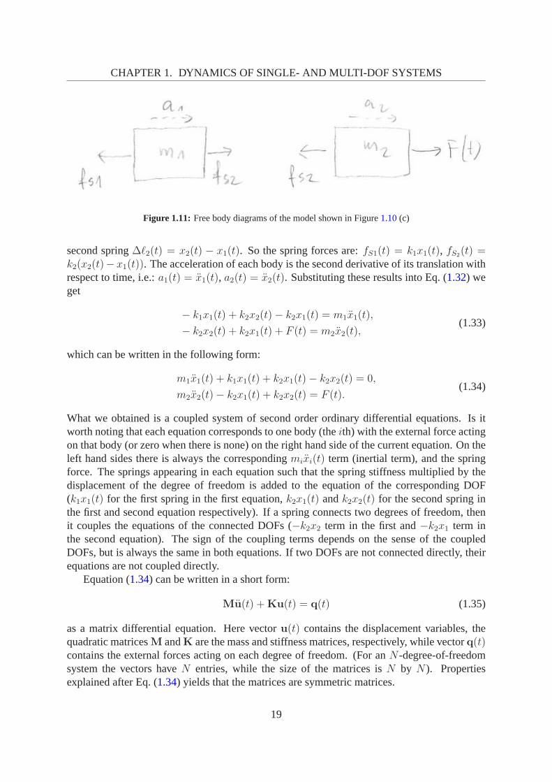
There are several ways to derive the equations of motion for aMDOF system. Here weshow one for the system on Figure1.10(c). The FBD of the system is shown in Figure1.11.The only displacement which is not constrained is the horizontal translation of the massesm1

andm2. Variablesx1(t) andx2(t) denote the translations of these masses, respectively. Thenumber of degrees of freedom is thereforetwo. Newton’s second law of motion is written forthe two masses:

− fS1(t) + fS2 = m1a1(t),

− fS2(t) + F (t) = m2a2(t).(1.32)

The forces in the linear springs depend on the elongation of each spring:fS1(t) = k1∆ℓ1(t),fS2(t) = k2∆ℓ2(t). For the first spring∆ℓ1(t) = x1(t) (assuming a fixed support) and for the

18


Figure 1.11: Free body diagrams of the model shown in Figure1.10(c)

second spring∆ℓ2(t) = x2(t) − x1(t). So the spring forces are:fS1(t) = k1x1(t), fS2(t) =

k2(x2(t)− x1(t)). The acceleration of each body is the second derivative of its translation withrespect to time, i.e.:a1(t) = x1(t), a2(t) = x2(t). Substituting these results into Eq. (1.32) weget

− k1x1(t) + k2x2(t)− k2x1(t) = m1x1(t),

− k2x2(t) + k2x1(t) + F (t) = m2x2(t),(1.33)

which can be written in the following form:

m1x1(t) + k1x1(t) + k2x1(t)− k2x2(t) = 0,

m2x2(t)− k2x1(t) + k2x2(t) = F (t).(1.34)

What we obtained is a coupled system of second order ordinary differential equations. Is itworth noting that each equation corresponds to one body (theith) with the external force actingon that body (or zero when there is none) on the right hand sideof the current equation. On theleft hand sides there is always the correspondingmixi(t) term (inertial term), and the springforce. The springs appearing in each equation such that the spring stiffness multiplied by thedisplacement of the degree of freedom is added to the equation of the corresponding DOF(k1x1(t) for the first spring in the first equation,k2x1(t) andk2x2(t) for the second spring inthe first and second equation respectively). If a spring connects two degrees of freedom, thenit couples the equations of the connected DOFs (−k2x2 term in the first and−k2x1 term inthe second equation). The sign of the coupling terms dependson the sense of the coupledDOFs, but is always the same in both equations. If two DOFs arenot connected directly, theirequations are not coupled directly.

Equation (1.34) can be written in a short form:

Mu(t) +Ku(t) = q(t) (1.35)

as a matrix differential equation. Here vectoru(t) contains the displacement variables, thequadratic matricesM andK are the mass and stiffness matrices, respectively, while vectorq(t)contains the external forces acting on each degree of freedom. (For anN -degree-of-freedomsystem the vectors haveN entries, while the size of the matrices isN by N ). Propertiesexplained after Eq. (1.34) yields that the matrices are symmetric matrices.

19


For the example shown in Figure1.10(c) the elements are:

M =

[m1 00 m2

],K =

[k1 + k2 −k2−k2 k2

],u(t) =

[x1(t)x2(t)

], u(t) =

[x1(t)x2(t)

],q(t) =

[0

F (t)

].

Similarly to the single-degree-of-freedom vibrations, wedivide the problems described byEq. (1.35) in two groups:

• if q(t) = 0, then the system of differential equations is homogeneous,and the resultingmotion is the free vibration.

• if q(t) 6= 0, then the system of differential equations is non-homogeneous, and it is calleda forced vibration.

Equations of motion of a two-storey frame

Let us analyse the equations of motion for a two-storey framestructure with a machineexerting a force on the upper level. The floors are rigid, so weonly have two degrees of free-dom. Figure1.12(a) shows the structure and one possible displacement system. Figure1.12(b) shows the free body diagrams for the same structure. The internal forcesfS1 (from thecolumns 1 and 1’) andfS2 (from the columns 2 and 2’) depend on the inter-storey driftsx1andx2 − x1, respectively. Assuming linear elastic columns one can calculate the equivalentstiffness coefficientsk1 andk2 for the columns on each level. Writing the equations of motionand the elements of the mass and stiffness matrices are left for the reader as an exercise.

Figure 1.12: Two-storey frame structure with rigid floors. (a) Mechanical model, (b) free body diagram.

Equations of motion with different variables

The deformed state of the structure in Figure1.12can be described not only with the globalcoordinates of each level, but with the inter-storey driftsas well. (In accordance with the earlier

20


notation we will denote them by∆ℓ1 and∆ℓ2.) Then we have to substitutex1(t) = ∆ℓ1(t),x2(t) = ∆ℓ1(t) + ∆ℓ2(t) and their derivatives into Eq. (1.32), and we get

−∆ℓ1(t) + k2∆ℓ2(t) = m1∆ℓ1(t),

− k2∆ℓ2(t) + F (t) = m2∆ℓ1(t) +m2∆ℓ2(t)

instead of Eq. (1.33). One can see, that using this description of the problem results non-symmetric mass- and stiffness matrices. This is due to the fact, that the equations still belongto the globalx1 andx2 translations, while our variables are the relative displacements∆ℓ1and∆ℓ2. Symmetry of the system matrices is often used during the calculations, so we canconclude, that this hybrid approach should be avoided if possible.

1.3.2 Free vibration of MDOF systems

During the analysis of a multi-degree-of-freedom system the solution of Eq. (1.35) followsthe same steps as for SDOF systems. The free vibration of the system is analysed using thecomplementary equation of Eq. (1.35). That is the homogeneous matrix differential equation

Mu(t) +Ku(t) = 0. (1.36)

We search for the solution of Eq. (1.36) in the form:

u(t) = u0 (a cos (ω0t) + b sin (ω0t)) , (1.37)

i.e. the displacement functionu(t) is assumed to be a product of a constant vectoru0 describingthe ratio of the degrees of freedom to each other and a harmonic function depending on time,natural frequencyω0 and two parametersa andb. The cases whenu0 = 0 or a = b = 0 wouldlead to the trivial solution of the Eq. (1.36). We are looking for the nontrivial solutions.

The second derivative of the displacement vectoru(t) is

u(t) = u0(−ω20) (a cos (ω0t) + b sin (ω0t)) .

We substituteu(t) andu(t) into the homogeneous differential equation (1.36):

Mu0(−ω20) (a cos (ω0t) + b sin (ω0t)) +Ku0 (a cos (ω0t) + b sin (ω0t)) = 0. (1.38)

This equation must hold for any timet, thus either(a cos (ω0t) + b sin (ω0t)) = 0, orMu0(−ω2

0) + Ku0 = 0. The equation(a cos (ω0t) + b sin (ω0t)) = 0 holds for all tonly with the trivial solutiona = b = 0, therefore the time-independent matrix equationMu0(−ω2

0) +Ku0 = 0 must be fulfilled, so it is rewritten in the more classical form(K− ω2

0M)u0 = 0. (1.39)

The above equation is a system of a homogeneous, linear equations, which is called a general-ized eigenvalue problem in mathematics. It has nontrivial solutions if and only if the matrix ofcoefficients is singular, or equivalently if and only if its determinant is zero. The equation:

det(K− ω2

0M)= 0

21


leads to a polynomial of degreeN for ω20 (whereN is the degree of freedom of the system).

Typically it hasN real solutions, denoted byω201 ≤ ω2

02 ≤, . . . ,≤ ω20N (i.e. the first one is the

smallest), and their positive square roots

ω01 ≤ ω02 ≤, . . . ,≤ ω0N

are the natural circular frequencies of the system. In the following steps we assume that all thenatural circular frequencies are different. We can defineN natural period of the system as:

T01 =2π

ω01

> T02 =2π

ω02

>, . . . , > T0N =2π

ω0N

.

In the next step we have to find the elements of vectoru0 of Eq. (1.37). Since we haveN natural circular frequencies, we will haveN different vectors. We will denote the vectorcorresponding toω0j by uj. The vectoruj must fulfill Eq. (1.39):

(K− ω2

0jM)uj = 0. (1.40)

Because of the matrix(K− ω2

0jM)

is singular,uj has onlyN −1 independent rows, i.e. it hasnot a uniqueuj solution. Ifuj is a solution, then the vectorαuj will be a solution for any real-valuedα. These vectors are the (generalized) eigenvectors of the system. The meaning of thejth eigenvectoruj is that if we displace the degrees-of-freedom in the same proportion as theelements of the eigenvector, then it will move such a way thatthe ratios of the displacementswill be the same during the motion with frequencyω0j. In this case the structure vibrates inits jth mode. The shape of the vibration (the modal shape) is described by the eigenvector (ormode vector).

Normalized eigenvectors

For further calculations we have to make the eigenvector unique. It can be done in differentways:

• making the first element of the vector be equal to 1,

• making the largest (in absolute value) element of the vectorbe equal to 1,

• making the length of the vector be equal to 1 (i.e.uTj uj = 1),

• making the vector be normalized to the mass matrix (i.e.uTj Muj = 1).

The first method is useful when the calculations are done by hand. The second method has animportant role in numerical solution of the eigenvalue problem. The third method would resultin possible small numbers in the case of a large system. The last method has positive conse-quences on further results so we assume that the eigenvectors are normalized to the mass matrix.(If we have a non-normalized eigenvectoruj, we can still calculate the productuT

j Muj = αj.It follows from the rules of matrix operations that the vector (1/

√αj)uj will be normalized to

the mass matrix.)

22


If we substitute thejth normalized eigenvector into Eq. (1.39), and multiply it with thetranspose of the same vector from the left we get:

uTj Kuj − ω2

0juTj Muj = 0.

Because of the eigenvector is normalized, the vector-matrix-vector product on the left hand sideequals 1, resulting in:

uTj Kuj = ω2

0j . (1.41)

Orthogonality of eigenvectors

Let us take two different natural circular frequenciesω0i 6= ω0j, and the correspondingeigenvectorsui anduj. Then it holds from Eq. (1.40) that

Kui = ω20iMui, (1.42)

Kuj = ω20jMuj. (1.43)

Multiplying Eq. (1.42) by uTj and Eq. (1.43) by uT

i from the left and subtracting the resultantequations lead to:

uTj Kui − uT

i Kuj = ω20iu

Tj Mui − ω2

0juTi Muj.

Due to the symmetry of matricesK andM

uTj Kui = uT

i Kuj, uTj Mui = uT

i Muj, (1.44)

so we have:0 =

(ω20i − ω2

0j

)uTj Mui.

The above equality only holds for differentω0i andω0j if:

uTj Mui = 0 . (1.45)

Dividing both side of Eq. (1.42) by ω20i, then multiplying the result byuT

j from the left,dividing both side of Eq. (1.43) by ω2

0j, then multiplying the result byuTi from the left, finally

subtracting the resultant equations lead to:

1

ω20i

uTj Kui −

1

ω20j

uTi Kuj = uT

j Mui − uTi Muj.

Due to Eq. (1.44) (1

ω20i

− 1

ω20j

)uTj Kui = 0,

which holds for different nonzeroω0i andω0j only when:

uTj Kui = 0 . (1.46)

We refer to this latter properties as the orthogonality of the eigenvectorsui anduj to themass matrix (Eq. (1.45)) and to the stiffness matrix (Eq. (1.46)).

23


General solution of the homogeneous differential equation

The general solution of the homogeneous differential equation Eq. (1.36) is constructedfrom the sum of the solutions corresponding to the eigenmodes:

u(t) =N∑

j=1

uj (aj cos (ω0jt) + bj sin (ω0jt)) . (1.47)

To find the parametersaj andbj we need the vector of velocities:

u(t) =N∑

j=1

ujω0j (−aj sin (ω0jt) + bj cos (ω0jt)) . (1.48)

Initial conditions of a multi-degree-of-freedom system are displacements and velocities of thedegrees of freedom at a given time instantt0:

u(t0) = u0, u(t0) = v0.

By substituting Eq. (1.47) and (1.48) into the above formula2N constraints are obtained whichcan be used to find the parametersaj and bj in the general solution Eq. (1.47). Using theorthogonal properties of the eigenvectors one can avoid thesolution of a system of2N linearequations. If we multiply these2N equations from the left byuT

j M, then we get

aj cos (ω0jt0) + bj sin (ω0jt0) = uTj Mu0,

ω0j (−aj sin (ω0jt0) + bj cos (ω0jt0)) = uTj Mv0,

so, varyingj from 1 toN we have to solveN system of2 linear equations instead of a systemof 2N equations for the coefficientsaj andbj.

The resultant motion will be the sum of harmonic vibrations,which is not necessarily aperiodic motion!

1.3.3 Harmonic forcing of MDOF systems (direct solution and modalanalysis)

The solution of forced vibration problems of multi-degrees-of-freedom systems follows asimilar schema as we experienced with the SDOF systems. The complete solution is the sumof the general solution of the complementary differential equation and a particular solutionof the nonhomogeneous differential equation. So the solution of Eq. (1.35) constructed fromEq. (1.47) and a particular solutionuf (t), which is the answer of the system to the forcing (thatis the subscriptf is for).

In this subsection we will give a possible solution of the problem, where the excitation forceis harmonic, i.e.q(t) can be written in the form:

q(t) = q0(t) sin (ωt) . (1.49)

24


Hereω is the circular frequency of the forcing, the vectorq0 is the amplitude of the forcing.Thus each DOF is excited with the same frequencyω. Is it worth mentioning, that a zeroextarnal force acting on a degree-of-freedom can be treatedas a harmonic force with zeroamplitude and arbitrary circular frequency.

Solving the nonhomogeneous equation we are looking only forthe steady-state part of thevibration. We show two possible solution method:

• direct solution,

• solution with the modal shape vectors and natural circular frequencies.

Direct solution

In the case of a direct solution we assume the particular solution of the form:

uf (t) = uf0 sin (ωt) , (1.50)

i.e. it is a harmonic response with the same harmonic term as the forcing, with constant ampli-tudes given in the vectoruf0.

The second derivative of Eq. (1.50) with respect to time is:

uf (t) = −ω2uf0 sin (ωt) . (1.51)

Substituting the load, the ansatz and its derivative (Eqs. (1.49), (1.50), and (1.51)) intoEq. (1.35) we get:

− ω2Muf0 sin (ωt) +Kuf0 sin (ωt) = q0 sin (ωt) . (1.52)

The above equation fulfills either ifsin (ωt) = 0, or if Kuf0 − ω2Muf0 = q0. Because theloading is a real, time dependent harmonic force, the termsin (ωt) cannot be zero for everytime instant. So, we can write the latter condition as:

(K− ω2M

)uf0 = q0. (1.53)

The solution of this non-homogeneous matrix differential equation for the amplitudeuf0 isneeded. The matrix of coefficients of Eq. (1.53) is quadratic, so it has a solution if and only ifthere exists its inverse matrix, i.e. the matrix is non-singular, or with other words, its determi-nant is nonzero. In that case we get the solution by multiplying both sides of Eq. (1.53) by theinverse(K− ω2M)

−1:uf0 =

(K− ω2M

)−1q0. (1.54)

The particular solution then can be written as:

uf (t) =(K− ω2M

)−1q0 sin (ωt) . (1.55)

This is the steady-state part of the vibration. We can see that each degree of freedom vibrateswith the same frequency. Without computing the inverse matrix, we cannot read out directlywhether a degree of freedom is in an in-phase or in an out-of-phase vibration.

25


We have to note that the non-existence of the inverse of the matrix (K− ω2M) means thatthe matrix is singular, i.e. its determinant equals zero. Butif det (K− ω2M) = 0, then thecircular frequency of forcing is one of the natural circularfrequencies of the system, i.e. thesystem is in the state of resonance. It means that if the frequency of forcing coincides with oneof the natural frequencies of the structure, then the directmethod gives an infinite amplitudeof the vibration. However, in real structures it does not occur, because there is always somedamping in the system.

Direct solution requires the calculation of the inverse of anN -by-N matrix. In general, therequired computational capacity increases proportional to the second- or third power ofN (theorder of the computational time isO (N2 ∼ N3)). Thus for large systems this method has avery high computational costs.

Modal analysis

Instead of the direct solution one can make use of the solutions of the unforced system, i.e.of the generalized eigenvalue problem Eq. (1.36). These solutions contain the natural circularfrequencies(ω01 , ω02, . . ., ω0N) and the corresponding mode shape vectors normalized to themass matrix(u1 , u2, . . ., uN). These eigenvectors are linearly independent and span anNdimensional linear space. Displacements are written as a linear combination of the normalisedmode shape vectors:

uf (t) =N∑

j=1

ujyj(t), (1.56)

where functionsyi(t) are the modal displacements. The modal shape vectors are invariant intime, so the second derivative of the displacement is:

uf (t) =N∑

j=1

uj yi(t). (1.57)

Substituting the load, the ansatz and its derivative (Eqs. (1.49), (1.56), and (1.57)) intoEq. (1.35) we get:

M

N∑

j=1

uj yj(t) +K

N∑

j=1

ujyj(t) = q0 sin (ωt) . (1.58)

Let us multiply both sides of Eq. (1.58) from the left byuTi . Using the orthogonality of the

eigenvectors (Eq. (1.45), and (1.46)) we only have nonzero values ifj = i:

uTi Muiyi(t) + uT

i Kuiyi(t) = uTi q0 sin (ωt) .

Moreover, the eigenvectors are normalized to the mass matrix, so:

uTi Mui = 1, uT

i Kui = ω20i,

which leads to the modal differential equation of vibration:

yi(t) + ω20iyi(t) = fi sin (ωt) , i = 1, 2, . . . , N. (1.59)

26


Herefi = uTi q0 is the modal amplitude of the harmonic excitation force.

For the particular solutionyif (t) of the non-homogeneous differential equation (1.59) weassume the solution in the harmonic form:

yif = yif0 sin (ωt) .

Its second derivative isyif = −ω2yif0 sin (ωt) .

Substitute these equalities into Eq. (1.59), and solve for arbitrary nonzerosin (ωt):

−ω2yif0 + ω20iyif0 = fi.

If ω = ω0i andfi 6= 0, then the frequencyω of the load and theith natural frequencyω0i

coincide, thus the system is in the state of resonance. It results in an infinitely largeith modaldisplacement. Otherwise, the unique, finite solution is:

yif0 = fi1

ω20i − ω2

= fi1

ω20i

1

1− ω2

ω20i

.

The last term in the above product is aresponse factorof an undamped oscillatory systemof natural circular frequencyω0i, excited by a harmonic force of circular frequencyω. Thiscoefficient is denoted byµi.

Let us summarise our results. In the absence of resonance thesteady-state part of the motion(the particular solution) can be written in the form:

uf (t) =N∑

i=1

1

ω20i

µiuiuTi q0 sin (ωt) . (1.60)

Checking the terms of the above equation from right to left we can conlude that the response isharmonic (sin (ωt)). For each mode the amplitude of the modal load (uT

i q0) is calculated. It isthen multiplied by the response factorµi depending on the ratio of the forcing and the naturalfrequency of the corresponding mode. Finally, the amplitude for each mode is divided by thesquare of the natural circular frequencyω2

0i of the mode. Due to this last term the effect ofhigher modes is usually much smaller, except for the case when the excitation occurs close toone of the resonant frequencies of the system.

Apparently, the solution of the problem with modal analysisseems to need even more com-putational effort, than that of the direct solution, beacuse we first have to solve a generalizedeigenvalue problem of the free vibration. For large systems, with many degrees of freedom,the solution of the eigenvelue problem has high computational needs. However, the parts fromhigher modes typically play a less significant role in the solution. There are numerical algo-rithms which do not compute all the eigenvalues and eigenvectors of the generalized eigenvalueproblem, nut only the first few of them. Later in the semester we will show that a reduced setof mode shape vectors calculated with these methods can be sufficient to approximate well themotion of the MDOF system.

27


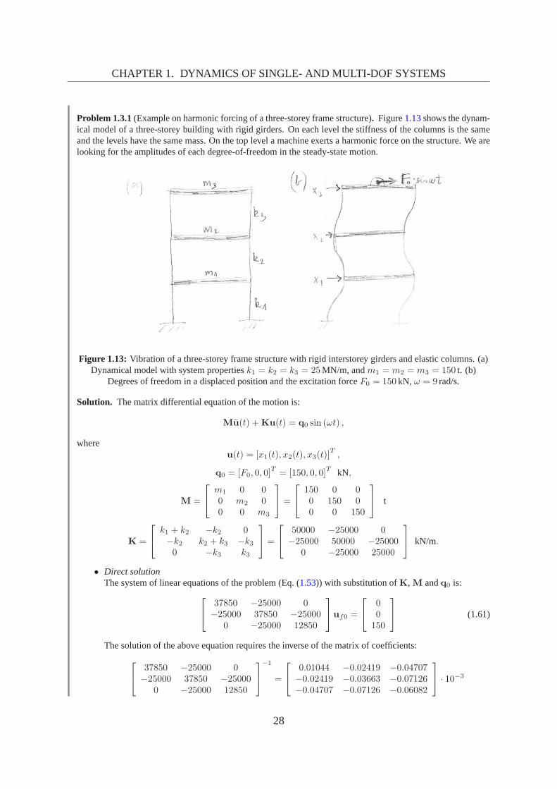
Problem 1.3.1(Example on harmonic forcing of a three-storey frame structure). Figure1.13shows the dynam-ical model of a three-storey building with rigid girders. Oneach level the stiffness of the columns is the sameand the levels have the same mass. On the top level a machine exerts a harmonic force on the structure. We arelooking for the amplitudes of each degree-of-freedom in thesteady-state motion.

Figure 1.13: Vibration of a three-storey frame structure with rigid interstorey girders and elastic columns. (a)Dynamical model with system propertiesk1 = k2 = k3 = 25MN/m, andm1 = m2 = m3 = 150 t. (b)

Degrees of freedom in a displaced position and the excitation forceF0 = 150 kN, ω = 9 rad/s.

Solution. The matrix differential equation of the motion is:

Mu(t) +Ku(t) = q0 sin (ωt) ,

whereu(t) = [x1(t), x2(t), x3(t)]

T,

q0 = [F0, 0, 0]T= [150, 0, 0]

T kN,

M =

m1 0 00 m2 00 0 m3

=

150 0 00 150 00 0 150

t

K =

k1 + k2 −k2 0−k2 k2 + k3 −k30 −k3 k3

=

50000 −25000 0−25000 50000 −25000

0 −25000 25000

kN/m.

• Direct solutionThe system of linear equations of the problem (Eq. (1.53)) with substitution ofK, M andq0 is:

37850 −25000 0−25000 37850 −25000

0 −25000 12850

uf0 =

00150

(1.61)

The solution of the above equation requires the inverse of the matrix of coefficients:

37850 −25000 0−25000 37850 −25000

0 −25000 12850

−1

=

0.01044 −0.02419 −0.04707−0.02419 −0.03663 −0.07126−0.04707 −0.07126 −0.06082

· 10−3

28


We have to multiply both sides of Eq. (1.61) from the left, resulting:

uf0 =

0.01044 −0.02419 −0.04707−0.02419 −0.03663 −0.07126−0.04707 −0.07126 −0.06082

· 10−3 ·

00150

uf0 =

−0.0070604−0.0106890.0091234

m. (1.62)

• Modal analysisThis solution requires the solution of the generalized eigenvalue problem:

(K− ω2

0M)u0 = 0. (1.63)

First we compute the eigenvalues of the problem. The condition we use is that the determinant of thematrix

(K− ω2

0M)

must be zero:

0 =

∣∣∣∣∣∣

50000− 150ω20 −25000 0

−25000 50000− 150ω20 −25000

0 −25000 25000− 150ω20

∣∣∣∣∣∣=

(50000− 150ω2

0

) ((50000− 150)

(25000− 150ω2

0

)− (−25000)(−25000)

)−

(−25000)((−25000)

(25000− 150ω2

0

)− 0)+ 0,

which results the following cubic equation forω20 :

−3375 · 103ω60 + 2812.5 · 106ω4

0 − 562.5 · 109ω20 + 15.625 · 1012 = 0.

There are three real valued solution of the above polynomialequation:

ω201 = 33.010, ω2

02 = 259.16, ω203 = 541.16,

resulting the natural circular frequencies in:

ω01 = 5.7455 rad/s, ω02 = 16.098 rad/s, ω03 = 23.263 rad/s.

(The corresponding natural periods are:T01 = 1.0936 s,T02 = 0.39030 s, andT03 = 0.27009 s.)

We show only the calculation of the first eigenvector (u1). It must fulfill the equation:(K− ω2

01M)u1 = 0,

which has the form after substitution of previous results:

50000− 150 · 33.01 −25000 0−25000 50000− 150 · 33.01 −25000

0 −25000 25000− 150 · 33.01

u11u12u13

= 0.

Here we assume a trial vector in the formu1 = [c1, 1, c3]T . So, with the first and the last equation we

avoid multi-variable equations. (It is not always possible, in that case we should solve a system of linearequations.) From the mentioned rows we have:

45048c1 − 25000 · 1 = 0 → c1 = 0.55496−25000 · 1 + 20048c3 = 0 → c3 = 1.2470

(The second equation is linearly dependent, but it can be used to check our results both for the naturalcircular frequency and the vector elements.)

29


Now the trial eigenvectoru1 is normalized to the mass matrixM. To do this, first we calculate:

α1 = uT1 Mu1 =

[0.55496 1 1.2470

]

150 0 00 150 00 0 150

0.554961

1.2470

[= 83.244 150 187.05

]

0.554961

1.2470

= 429.44,

then the normalized shape vector correspondiong to the firstnatural mode will be:

u1 =1√α1

u1 =[0.02678 0.04826 0.06017

]T. (1.64)

The steps between Eq. (1.13) and (1.64) must be repeated forω02 and forω03 as well, to calculate thecorresponding normalized eigenvectors. The final results of that calculations are:

u2 =[0.06017 0.02678 −0.04826

]T

andu3 =

[−0.04826 0.06017 −0.02678

]T.

Figure1.14shows the deformed shape of the structure corresponding to the three modal vector. Nowwe can calculate the amplitude vector of the steady-state vibration using the formula of Eq. (1.60). Theterms are summarized in Table1.1.

Figure 1.14: Mode shapes of the three-storey structure of Figure1.13corresponding to the naturalcircular frequencies (a)ω01 = 5.7455 rad/s, (b)ω02 = 16.098 rad/s, and (c)ω03 = 23.263 rad/s.

i 1 2 3

uTi q 9.026 -7.238 -4.017

µi -0.6879 1.4556 1.176

1ω2

0i

µi -0.02084 0.005613 0.002173

1ω2

0i

µiuTi q -0.1881 -0.04053 -0.00873

Table 1.1: Harmonic forcing of a three-storey structure. Modal loads,coefficients of resonance, thiscoefficient divided by the square of theith natural circular frequency, participation of the mode inthe

steady-state vibration.

30


From Table1.1we can see, that this specific loading has a projection in the same order of magnitude ineach mode, and the coefficient of resonance does not change this proportion much. Contrary to this, thewhole participation of the first mode is 4.5 times higher thanthe participation of the second mode, and20 times higher, than that of the third mode, due to the division byω2

0i.

The amplitude vector of the steady-state vibration will be:

uf0 = −0.1881u1 − 0.04053u2 − 0.00873u3 =

−0.0070604−0.0106890.0091234

m. (1.65)

For both solution methods we can conclude, that in the steady-state vibration each level oscillates in a cm range,the lower two levels are out-of-phase, the upper level is in-phase with the forcing.

1.3.4 Approximate solution of the generalized eigenvalue problem (Ritz-Rayleigh’s method)

We have seen already, that a higher natural frequency of a multi-degrees-of-freedom systemplays an important role only if the forcing has a frequency close to that natural frequency. Inpractical problems, the first few natural modes are sufficient to describe the vibration of thestructure. On the mode shape level, a mode vector of a higher natural frequency results morechanges in the sense of displacements of DOFs. So, thesimplermode shapes correspond tolower natural frequencies, and an eigenvector (normalizedto the mass matrix) can be used as abase for the calculation of the eigenvalue (see Eq. (1.41)).

The Rayleigh quotient

Approximate solutions can be obtained by guessing the mode shape vector of the structure,and finding the corresponding natural frequency. This is theopposite of the classical solutionof the generalized eigenvalue problem, where we started with finding the eigenvalues from thepolynomial equation defined by the determinant of the matrixof coefficientsK − ω2

0M of thehomogeneous equation, and then the eigenvectors were calculated.

Let us assume, thatv is a vector ofN element. We define the Rayleigh quotient as:

R =vTKv

vTMv. (1.66)

Altough we do not know the eigenvectors,v can be written as a linear combination of themwith coefficientsαj:

v =N∑

j=1

αjuj.

Let us expand the denominator and the numerator of Eq. (1.66). The denominator can bewritten as:

vTMv =

(N∑

j=1

αjuj

)T

M

(N∑

i=1

αiui

)=

N∑

j=1

N∑

i=1

αjαiuTj Mui.

31


Orthogonality of the normalized eigenvectors (Eq. (1.45)) implies that the quadratic productuTj Mui = 1 if j = i and zero otherwise, thus

vTMv =N∑

j=1

α2j .

The numerator of Eq. (1.66) can be written as:

vTKv =

(N∑

j=1

αjuj

)T

K

(N∑

i=1

αiui

)=

N∑

j=1

N∑

i=1

αjαiuTj Kui.

Orthogonality of the normalized eigenvectors (Eq. (1.46)) implies that the quadratic productuTj Kui = ω2

0j if j = i and zero otherwise. Therefore

vTKv =N∑

j=1

α2jω

20j.

The above formula can be expanded to:

vTKv =N∑

j=1

(α2j

(ω20j − ω2

01

)+ α2

hω201

)=

N∑

j=1

α2j

(ω20j − ω2

01

)+

N∑

j=1

α2jω

201.

The first summation term is zero ifj = 1, so we got finally:

vTKv =N∑

j=1

α2jω

201 +

N∑

j=2

α2j

(ω20j − ω2

01

).

If we write the result into the definition of the Rayleigh quotient (1.66) we get:

R =

N∑j=1

α2jω

201 +

N∑j=2

α2j

(ω20j − ω2

01

)

N∑j=1

α2jω

201

= ω201 +

N∑j=2

α2j

(ω20j − ω2

01

)

N∑j=1

α2jω

201

. (1.67)

The sum on the right hand side of Eq. (1.67) contains only positive numbers (here we remind,thatω01 is the smallest natural frequency), or zeros (if a specificαj is zero). So we can conclude,that the Rayleigh quotient is always higher than, or equal to the square of the first naturalcircular frequency. The accuracy of the result depends naturally on the initial guess on themode shape vector (v): the closer the guessed shape vectorv is to the exact oneu1, the morepreciseω01 is.

Seeding theω20N element instead ofω2

01 results in a proof for the Rayleigh quotient to besmaller than, or equal to the square of the highest natural circular frequency.

32


Problem 1.3.2(Example on finding an approximate solution for a two-storeyframe). Find an approximatesolution of the first natural circular frequency of the two-storey structure shown in Figure1.12. The massesof the storeys arem1 = m2 = 2 t, and the stiffness of the columns is given by spring stiffnessesk1 = k2 =

50 kN/m. The first mode shape should be assumed as:v =[1 2

]T

Solution. The system has the following mass and stiffness matrices:

M =

[2 00 2

],K =

[100 −50−50 50

].

The numerator and the denominator of the Rayleigh quotient are:

vTMv =[1 2

] [ 2 00 2

] [12

]=[2 4

] [ 12

]= 10,

vTKv =[1 2

] [ 100 −50−50 50

] [12

]=[0 50

] [ 12

]= 100.

So, the Rayleigh quotient is:

R =vTKv

vTMv=

100

10= 10,

resulting in the approximation:ω201 ≤ 10, ω01 ≤ 3.162 rad/s.

Exercise1.3.1. Find first natural circular frequencyω01 of the above problem with the exact first mode shapevector:

u1 =[1 1.618

]T.

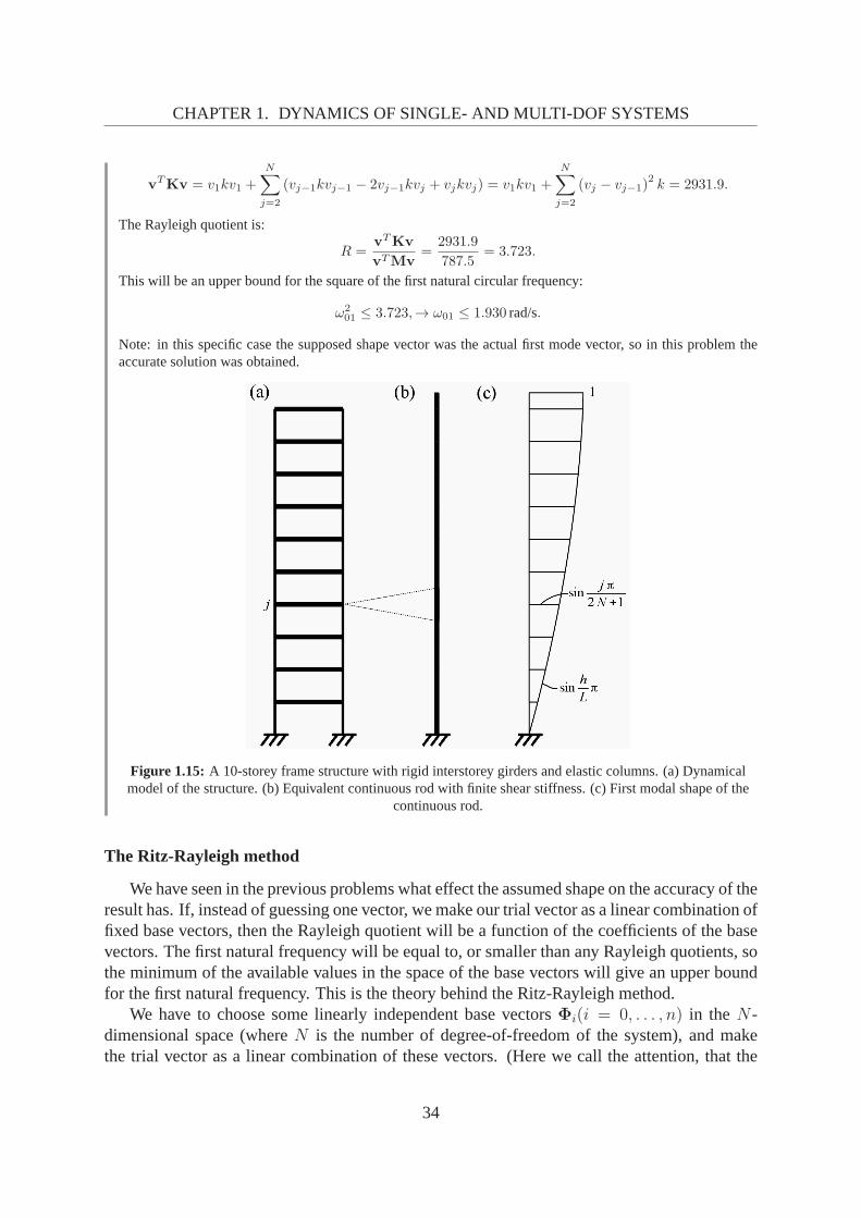
Problem 1.3.3(Example on finding an approximate solution for a multi-storey frame). Let us find the firstnatural circular frequency of a 10-storey frame. (See Figure 1.15(a).) The inter-storey stiffnesses and the levelmasses are the same on each level,m = 150 t andk = 25000 kN/m respectively.

Solution. The mass matrix of the structure is a10 × 10 diagonal matrix, where each element equalsm. Thestiffness matrix is

K =

k + k −k 0 . . . 0

−k k + k −k . .....

0 −k k + k. .. 0

.... . .

. . .. .. −k

0 . . . 0 −k k

.

It is a crucial step of the method to find a good assumption of the trial vector. During the drift of the storeys,the rigid girders are staying horizontal, and so the structure follows a pattern of displacements similar to a rodwith finite shear stiffness. The frame can be treated as a discrete model of the sheared (continuous) column(Figure1.15(b)). A sheared rod has a modal shape of a sinusoidal functionwith a zero value at the bottom anda zero tangent at the free end. Similar displacement vector can be used with:

vj = sinjπ

2N + 1, j = 1, . . . , N.

Displacements are shown in Fig.1.15 (c). The numerator and the denominator of the Rayleigh quotientare:

vTMv =

N∑

j=1

vjmvj = m

N∑

j=1

sin2jπ

2N + 1= m

2N + 1

4= 787.5,

33


vTKv = v1kv1 +N∑

j=2

(vj−1kvj−1 − 2vj−1kvj + vjkvj) = v1kv1 +N∑

j=2

(vj − vj−1)2k = 2931.9.

The Rayleigh quotient is:

R =vTKv

vTMv=

2931.9

787.5= 3.723.

This will be an upper bound for the square of the first natural circular frequency:

ω201 ≤ 3.723,→ ω01 ≤ 1.930 rad/s.

Note: in this specific case the supposed shape vector was the actual first mode vector, so in this problem theaccurate solution was obtained.

Figure 1.15: A 10-storey frame structure with rigid interstorey girdersand elastic columns. (a) Dynamicalmodel of the structure. (b) Equivalent continuous rod with finite shear stiffness. (c) First modal shape of the

continuous rod.

The Ritz-Rayleigh method

We have seen in the previous problems what effect the assumedshape on the accuracy of theresult has. If, instead of guessing one vector, we make our trial vector as a linear combination offixed base vectors, then the Rayleigh quotient will be a function of the coefficients of the basevectors. The first natural frequency will be equal to, or smaller than any Rayleigh quotients, sothe minimum of the available values in the space of the base vectors will give an upper boundfor the first natural frequency. This is the theory behind theRitz-Rayleigh method.

We have to choose some linearly independent base vectorsΦi(i = 0, . . . , n) in theN -dimensional space (whereN is the number of degree-of-freedom of the system), and makethe trial vector as a linear combination of these vectors. (Here we call the attention, that the

34


inequalityn + 1 ≤ N , must hold, otherwise the vectorΦi can not make a base of theN -space.) We want to make ourv unique among all vectors parallel with it. We have seen,that normalizing the eigenvector to the mass matrix is a verypractical way, but now it gives anonlinear constraint to the system, and that makes difficultto use. Instead of that, we set thecoefficient of one base vector(Φi) equal to one, and write the trial vector as:

v(c1, . . . , cn) = Φ0 +n∑

i=1

ciΦi.

Using this trial vector the Rayleigh quotient will depend on the variablesc1, . . ., cn:

R(c1, . . . , cn) =vT (c1, . . . , cn)Kv(c1, . . . , cn)

vT (c1, . . . , cn)Mv(c1, . . . , cn).

We are looking for the possible smallest R in the space of the vectorsΦ1, . . ., Φn:

R(c1, . . . , cn) = min!

• If n = 1:The quotient depends on one single variable. At the minimum the first derivative van-ishes:

dR(c1)

dc1= 0. (1.68)

The solution of the (nonlinear) equation (1.68) results in a possible best result for the trialvector coefficientc1 in the space of the base vectors.

• If n > 1:The quotient depends on multiple variables. At the minimum the gradient of the quotientis zero:

∂R(c1, . . . , cn)

∂ci= 0. i = 1, . . . , n, (1.69)

which is a nonlinear system of equations forn variables. This type of equations doesnot necessarily have a unique solution, thus solution method must be chosen accordingto this.

We mention here, that the Ritz-Rayleigh method is capable of finding the exact solution ifn + 1 = N , i.e., if the base vectorsΦi(i = 0, . . . , n) span the wholeN space. Otherwise,for the trial vector the method minimizes the error to the theexact solution, i.e. it finds theprojection of the exact solution on the space spanned by the base vectorsΦi(i = 0, . . . , n), andgives the corresponding Rayleigh quotient.

Problem 1.3.4(Exact solution of a two-storey frame). Find the exact solution for the first natural circularfrequency of the two-storey structure of Problem1.3.2.

35


Solution. Let us assume the trial vector asv(c1) =[1 c1

]T, i.e. we chose the base vectors:

Φ0 =

[10

], Φ1 =

[01

]

Heren = 1 andN = 2, so1 + 1 = 2, i.e. we will get the exact solutions.The numerator and the denominator of the Rayleigh quotient are:

vT (c1)Mv(c1) =[1 c1

] [ 2 00 2

] [1c1

]=[2 2c1

] [ 1c1

]= 2 + 2c21.

vT (c1)Kv(c1) =[1 c1

] [ 100 −50−50 50

] [1c1

]=[1 c1

] [ 100− 50c1−50 + 50c1

]

= 100− 100c1 + 50c21.

The resulting Rayleigh quotient is:

R(c1) =vT (c1)Kv(c1)

vT (c1)Kv(c1)=

100− 100c1 + 50c212 + 2c21

.

The first derivative is:

dR(c1)

dc1=

(−100 + 100c1)(2 + 2c21

)−(100− 100c1 + 50c21

)(4c1)

(2 + 2c21)2

=200

(c21 − c1 − 1

)

4 (c41 + 2c21 + 1)= 0

It is sufficient, if the nominator equals zero, so the coefficient c1 we are looking for is the solution of thequadratic equation:

c21 − c1 − 1 = 0.

There are two solutions:(1 +

√5)/2 and

(1−

√5)/2. If we substitute them back to the Rayleigh quotient,

the first one results the smaller number, so this will be the first mode

R(1.618) = 9.549 → ω01 = 3.090 rad/s,

while for the second solution we get

R(−0.618) = 65.45 → ω01 = 8.090 rad/s.

The resultant modal shape vectors are:

v1 =

[1

1.618

], v2 =

[0

−0.618

].

Problem 1.3.5(Exact solution for a three-storey structure). Find the exact solution for the first natural circularfrequency of the three-storey structure of Problem1.3.1.

Solution. First we repeat the matrices of the system from Problem1.3.1:

M =

150 0 00 150 00 0 150

,

36


K =

50000 −25000 0−25000 50000 −25000

0 −25000 25000

.

Let us assume the trial vector asv(c1, c2) =[1 c1 c2

]T, i.e. we chose the base vectors:

Φ0 =

100

, Φ1 =

010

, Φ2 =

001

Heren = 2 andN = 3, so2+1 = 3, i.e. the Ritz-Rayleigh method leads to the exact solutionsof the problem.The numerator and the denominator of the Rayleigh quotient are:

vT (c1, c2)Mv(c1, c2) =[1 c1 c2

]

150 0 00 150 00 0 150

1c1c2

=[1 c1 c2

]

150150c1150c2

= 150

(1 + c21 + c22

),

vT (c1, c2)Kv(c1, c2) =[1 c1 c2

]

50000 −25000 0−25000 50000 −25000

0 −25000 25000

1c1c2

=[1 c1 c2

]

50000− 25000c1−25000 + 50000c1 − 25000c2

−25000c1 + 25000c2

= 25000(2− 2c1 + 2c21 − 2c1c2 + c22

).

The resulting Rayleigh quotient is

R(c1, c2) =25000

(2− 2c1 + 2c21 − 2c1c2 + c22

)

150 (1 + c21 + c22)(1.70)

The first partial derivatives are:

∂R(c1, c2)

∂c1= 0,

∂R(c1, c2)

∂c2= 0.

The partial derivatives result a cumbersome system of two equations. However, the solution can be calculatednumerically, resulting in the following solution pairs:

• c1 = 1.802, c2 = 2.247,

• c1 = 0.445, c2 = −0.802,

• c1 = −1.247, c2 = 0.555.

These points are on the surface defined by the Rayleigh quotient over the(c1, c2)-plane (see Eq. (1.70)). Theshape of the surface is shown in Figure1.16.

To decide, which one of the above three solution pairs leads to the first natural frequency, we have twooptions:

• We decide which one of the solution pairs correspond to the minimum point of the surface given by thefunctionR (c1, c2).

• We calculate the Rayleigh quotient with the solution pointsand pick the smallest one.

37


Either way, the smallest possible Rayleigh quotient of thisproblem , and so the square of the first naturalcircular frequency is

R = 33.01,→ ω01 = 5.745 rad/s,

which is the same as the analytical result.

Figure 1.16: Rayleigh quotient of Problem1.3.1

Exercise1.3.2. Find an approximate solution of the above problem for the first natural circular frequencyω01

using the base vectors:

Φ0 =

11.50

, Φ1 =

001

.

38


1.4 Summation theorems

Let us study the undamped free vibration of a MDOF, linear mechanical system describedby the matrix differential equation

Mu(t) +Ku(t) = 0.

It leads to the generalised eigenvalue problem(K− ω2

0M)u0 = 0, (1.71)

the smallest eigenvalue of which isω201, the square of the lowest natural circular frequency

of the system. Here bothM andK are constant, symmetric, real valued,N -by-N matrices,calledlinear, symmetric operatorsin mathematics. We deal with simple models of engineeringstructures which are not statically overdeterminate. Thenthe mass matrixM and the stiffnessmatrixK arepositive definite. 1 Physically it means that the kinetic and elastic energies ofthestructure must be positive due to any displacements.

These properties of the system allow us to make use of a few summation theorems. Thesetheorems are used to get approximate estimates of the lowestnatural circular frequencyω01 ofa structure by combining natural frequencies of different subproblems. Here we do not providethe reader with the proofs of the theorems, they can be found in the literature (for instance in[9]), but we show some simple examples for their applications.

1.4.1 Dunkerleytheorem

Let us decompose themass matrixas

M =n∑

j=1

Mj,

whereMj (j = 1, 2, . . . , n). We write the generalised eigenvalue problem(K− ω2Mj

)u = 0

and denote its smallest eigenvalue byω2j for j = 1, 2, . . . , n.

Using these values theDunkerleyformula

1

ω201

≤n∑

j=1

1

ω2j

(1.72)

allows us to approximate the lowest natural circular frequency ω01 of the original problem.From this the first natural period of vibration is

T 201 ≤

n∑

j=1

T 2j .

1Matrix A is positive definite ifvTAv ≥ αvTv for someα > 0, which implies that all the eigenvalues ofA

are positive.

39


This theorem states that the reciprocal of the square of the smallest natural circular fre-quency of the structure is not greater than the sum of reciprocals of the squares of the smallestnatural circular frequencies of the same structure subjected to subsystems of the mass.

This approximation underestimates the natural circular frequency and overestimates thenatural period of vibration, thus it shows the structuresofterthan in reality. The usage of thissummation theorem is preferable if the structure is such that its mass can be split into partsand the natural circular frequencies of the resulting substructures are easy to compute. Theapplication of this theorem is referred to as the “method of split the masses”. The closer theeigenshapes of the substurctures are, the more precise thisapproximation is.

Problem 1.4.1(Estimation of the natural circular frequency usingDunkerleytheorem). There is a clamped rodof length3h and bending stiffnessEI. The total mass of the rod is concentrated at three points of the rod: massm1 is at the free end, massm2 is ath from the free end, and massm3 is at2h from the free end, as it is shownin Figure1.17(a). Estimate the first natural circular frequency of the structure!

Solution. We make use of the method of split the masses. First we takem2 andm3 to be equal to zero andcompute the natural circular frequencyω1 of a clamped, massless rod with one lumped massm1 at its top(see Figure1.17(b)). The compliancef1 of this structure equals to the horizontal translation of the top due toa unit force acting horizontally at the top. We compute the displacement using the theorem of virtual forces(Castigliano’s method).

The spring stiffnessk1 is the inverse of the compliance, and the square of the natural frequency isω21 =

k1/m1. Then, we setm1 andm3 to zero and compute the natural circular frequencyω2 of the clamped rod withonly one massm2 ath from the top (see Figure1.17(c)) in a similar way. Finally,m1 andm2 are set to zeroandω3 is computed. A brief summary of the computation is as follows:

f1 =1

2EI3h2 2

33h = 9

h3

EI→ k1 =

1

9

EI

h3→ ω2

1 =1

9

EI

h3m1

,

f2 =1

2EI2h2 2

32h =

8

3

h3

EI→ k2 =

3

8

EI

h3→ ω2

2 =3

8

EI

h3m2

,

f3 =1

2EIh2 2

3h =

1

3

h3

EI→ k3 = 3

EI

h3→ ω2

3 = 3EI

h3m3

.

The estimation of the first natural circular frequency of theoriginal structure is based on (1.72):

1

ω201

≤ h3

EI

9m1 +

8

3m2 +

1

3m3

, thus

ω01 ≥√

3EI

h327m1 + 8m2 +m3, and

T01 ≤ 2π

√h327m1 + 8m2 +m3

3EI.

40


m1

m2

m3

EI

hh

h

(a)

m2F=1

M

2h

m1

EI3h

F=1

M

3h

(b)

F=1

M

h

(d)

EI

m3

h

(c)

EI

2h

Figure 1.17: (a) A clamped rod of length3h and bending stiffnessEI with its mass concentrated at threepoints of equal distancesh. (b) The case when massesm2 andm3 are zero with the corresponding

substructure and the bending moment diagram due to a horizontal unit forceF = 1 at the top. (c) The casewhen massesm1 andm3 are zero with the corresponding model and the bending momentdiagram due to ahorizontal unit forceF = 1 acting ath from the top. (d) The case when massesm1 andm2 are zero and the

substructure with the bending moment diagram due to a unit forceF = 1 acting at2h from the top.

41


1.4.2 Southwelltheorem

Let us write thestiffness matrixin the form

K =n∑

j=1

Kj.

It is assumed thatKj (j = 1, 2, . . . , n) possesses the same properties asK (i.e. symmetric andpositive definite). The generalised eigenvalue problem

(Kj − ω2M

)u = 0, j = 1, 2, . . . , n (1.73)

hasN eigenvalues for eachj. The smallest of them is denoted byω2j .

The lowest natural circular frequencyω01 of the original problem can be approximatedusing theSouthwellformula

ω201 ≥

n∑

j=1

ω2j . (1.74)

The first natural period of vibration is estimated as

T 201 ≤

(n∑

j=1

1

T 2j

)−1

.

Thus this formula states that if the stiffness of the structure is composed of parts, then thesquare of the smallest natural circular frequency of the structure is not less than the sum of thesquares of the smallest natural circular frequencies corresponding to the partial stiffnesses.

The formula underestimates the natural circular frequencyof the structure, i.e. the resultshows the structuresofterthan in reality. We refer to this theorem as the “effect of stiffening”.Let a structure haveS stiffness parameters. We can group these parameters inton sets. If thestructuredoes not become statically overdeterminatewhen all but one of the stiffness parametersets equalzero, then theSouthwelltheorem can be applied. Practically, wedecreaseall but thejth sets of stiffness parameters tozeroand then compute the corresponding smallest naturalcircular frequencyωj for j = 1, 2, . . . , n. Finally, we apply theSouthwellformula (1.74).

Problem 1.4.2(Estimation of the natural circular frequency usingSouthwelltheorem). There is a rigid roof ofmassm supported by two clamped rods of lengthh and bending stiffnessesEI1, EI2. The rods are connectedto the roof through hinges and the mass of the rods is neglected. In addition, there is a linear spring of stiffnessk attached to the roof. The model is shown in Figure1.18(a). Estimate the first natural circular frequency ofthe structure!

Solution. We applySouthwelltheorem, since the structure is such that if we set any 2 stiffness parameters outof EI1, EI2, or k, to zero, then the structure remains stable. First we takeEI2 andk to be equal to zero andcompute the natural circular frequencyω1 of a clamped, massless rod of lengthh and bending stiffnessEI1with one lumped massm at its top (see Figure1.18(b) and (e)). Then, we takeEI1 andk to be equal to zeroand compute the natural circular frequencyω2 of a clamped rod of lengthh and stiffnessEI2 with the massm at its the top (see Figure1.18(c) and (e)) in a very similar way. Finally,EI1 andEI2 are taken to be zero

42


andω3 is computed simply: in this case the massm is supported by a spring of stiffnessk, soω23 = k/m. The

computation ofω21 andω2

2 briefly is

f1 =1

2EI1

2

3h3 =

h3

3EI1→ k1 =

3EI1h3

→ ω21 =

3EI1h3m

,

f2 =1

2EI2

2

3h3 =

h3

3EI2→ k1 =

3EI2h3

→ ω22 =

3EI2h3m,

1 2

(c)

EI =0 EIh

m k=0

1 2

(a)

EI EIh

m k

1 2EI EI =0h

m k=0

(b)

1 2

(d)

EI =0 EI =0h

m k

F=1

M

h

(e)h

Figure 1.18: (a) Model of a rigid roof of massm supported by a linear spring of stiffnessk and by twoclamped, massless rods of equal lengthh and bending stiffnessesEI1 andEI2. (b) The case when the

stiffness parametersEI2 andk are set to zero. (c) The case whenEI1 andk are set to zero. (d) The case whenEI1 andEI2 are taken to be zero. (e) A clamped rod of lengthh and its bending moment diagram due to a

horizontal unit force at the top.

The estimation of the first natural circular frequency of theoriginal structure following (1.74) is

ω201 ≥ 3EI1

h3m+

3EI2h3m

+k

m, thus

ω01 ≥√

1

m

3

h3EI1 + EI2+ k

, and

T01 ≤ 2π√m

3

h3EI1 + EI2+ k

.

43


1.4.3 Foppl–Papkovichtheorem

Let the eigenvectoru0 of (1.71) be a sum of pairwiseK-orthogonal vectorsuj, j =1, 2, . . . , n. (Vectorsuj andui areK-orthogonal ifuT

j Kui = 0.) Practically it means thatthe deformation modes of the structure are independent, i.e. the strain energy of the structuredoes not contain mixed terms of the deformation modes.

The smallest eigenvaluesω2j of the generalised eigenvalue problems

(K− ω2M

)uj = 0, j = 1, 2, . . . , n (1.75)

are the basis of the approximation ofω01. The formula we can use is

1

ω201

≤n∑

j=1

1

ω2j

. (1.76)

From this the first natural period of vibration is

T 201 ≤

n∑

j=1

T 2j .

This approach again shows the structuresofterthan it is.We refer to this theorem as the “method of split rigidities”, or partial rigidizing. If a struc-

ture hasS stiffness parameters, then we can group them inton sets. If the structurebecomesstatically overdeterminatewhen all but one of the stiffness parameter sets equalzero, then theFoppl–Papkovichtheorem can be applied. In practice, weincreaseall but thejth sets of stiff-ness parameters toinfinity and compute the corresponding smallest natural circular frequencyωj for j = 1, 2, . . . , n. Then we can utilise formula (1.76).

Problem 1.4.3(Estimation of the natural circular frequency usingFoppl–Papkovichtheorem). There is a mass-less rod of lengthh and bending stiffnessEI. The top end of the bar is free and a massm is attached to it,while the bottom end is connected to a fixed hinge and equippedwith a linear rotational spring of stiffnesss.See the model in Figure1.19(a). Estimate the first natural circular frequency of the structure!

Solution. The structure becomes statically overdeterminate if either one of its stiffness parameters (EI or s)is set to zero. Therefore, we apply theFoppl–Papkovichtheorem. First we stiffen the rotational spring, i.e. wetakes → ∞, which implies that the bar is rigidly clamped at the bottom.Now we compute the compliancef1(the translation of the top of the bar caused by a horizontal unit force), then the stiffness isk1 = 1/f1, and thenatural circular frequency equals toω2

1 = k1/m. See Figure1.19(b). Next we stiffen the bar against bendingdeformation, i.e.EI → ∞. Now the rod is a rigid body capable to rotate about the hinge at the bottom end,which generates a moment in the rotational spring. The compliancef2 is the horizontal translation of the topend caused by a horizontal unit force. The moment of equilibria of the structure isφs − Fh = 0 (assumingsmall displacements), as it is indicated in Figure1.19 (c). From this, if we takeF = 1, the rotation of therigid body isφ = h/s, and the horizontal translation of its top isf2 = φh = h2/s. (Again, we consider smalldisplacements.) The stiffnessk2 is the inverse off2, andω2

2 = k2/m. This computation is summarised below.

f1 =1

2EI

2

3h3 =

h3

3EI→ k1 =

3EI

h3→ ω2

1 =3EI

h3m,

f2 =h2

s→ k2 =

s

h2→ ω2

2 =s

h2m.

44


M

h

EIh

m F=1

EIh

f2

(b)

(c)

h

s

F=1

φ

F=1

Fh=s φ

φ

EIh

s

m

8

EIh

(a)

s

m

Figure 1.19: (a) A straight, massless rod of lengthh and bending stiffnessEI carrying a lumped massm atthe top, connected to a fixed hinge and a rotational spring of stiffnesss at the bottom. (b) The case when

s→ ∞ (rigidly clamped elastic rod) and the bending moment diagram due to a horizontal unit force acting atthe top. (c) The case whenEI → ∞ (elastically clamped rigid bar) and the free body diagram due to a

horizontal unit force.

The estimation of the first natural circular frequency of theoriginal structure using Eq. (1.76) is

1

ω201

≤ h3m

3EI+h2m

s, thus

ω01 ≥ 1√h3m

3EI+h2m

s

, and

T01 ≤ 2π

√h3m

3EI+h2m

s.

45

CHAPTER 2. DYNAMICS OF SLENDER CONTINUA

Chapter 2

Dynamics of slender continua

Main load bearing members of engineering structures often have one significant dimension:the extent of the member along this direction is larger with at least one order of magnitude thanin other (orthogonal) directions. The behaviour of theseslendermembers can be characterizedby fewer variables, than needed for a complete three-dimensional description. In this chapterwe derive the equation of motion of some specificslender continuum rods, give the solution forthe free vibrations and, in some cases, forced vibrations are also studied.

First we collect the assumptions used hereafter for the studied rods. Since in engineeringpractice the most commonly used structural element is theprismatic rod, which is a slender,straight rod of uniform cross-sections, we restrict our investigations on this type of rods. It isassumed to be homogeneous, isotropic, and linearly elastic. We neglect the effect of damping.The axis of the rod in the stress-free state is the straight line connecting the centroids of thecross-sections. In the stress-free state, the axis of the rod coincides with axisx of a left handedCartesiancoordinate system (see Figure2.1 (a)). The rod obeys the principle of planar cross-sections: during the deformation every cross-section remains plane and undistorted. The cross-section of the rod is assumed to be reflection symmetric to axis y. The displacements areconsidered to be small. Thelengthof the studied rod is denoted byℓ, its cross-sectional areaisA, thesecond moment of the cross-sectionwith respect toz is I, and thepolar inertia of thecross-sectionwith respect to axisx is I0. The material of the rod is characterised by: themassdensity , theYoung’s modulusE, theshear modulusG, and thePoisson’s ratioν. 1 Themassper unit lengthof the rod isµ = A.

We analyse the following simple vibration modes:

• Longitudinal vibration of prismatic bars. The rod deforms along its axisx, while all thecross-sections remain parallel, thus their motion can be characterised by the translationu(x, t) of the rod axis. The only non-zero internal force in this caseis the normal forceN . A simple model is shown in Figure2.1(a), and free vibrations are solved using bothstanding and travelling waves in Section2.1.

• Torsional vibration of prismatic shafts. The cross-sections of the rod rotate about axisx and this rotation is denoted byϕx(x, t). The cross-sections remain parallel. The only

1AlthoughE,G, andν are not independent:E = 2(1 + ν)G.

46


non-zero internal force is the torqueT . The free vibration of this structure is discussedin Section2.2.

• Shear vibration of prismatic beams. The rod deforms along axisy. The non-zero internalforces in this case are the shearV and the bending momentM , but the rod is assumed tobeunbendable. Thus all the cross-sections remain parallel, their motioncan be describedby the translationv(x, t) of the rod axis. A simple model is shown in Figure2.3(a), andthe solution of the free vibration is given in Section2.3.

• Transverse vibration of prismatic beams. The rod axis translates alongy and the cross-sections rotate about axisz. The translation and the rotation are denoted byv(x, t) andϕ(x, t), respectively. The non-zero internal forces in this case are the shearV and thebending momentM , but rod is assumed to beunshearable, thereforev(x, t) andϕ(x, t)are not independent. A simple model is shown in Figure2.5(a), and a thorough vibrationanalysis is given in Section2.4.

2.1 Longitudinal vibration of prismatic bars

In this section we analyse the longitudinal vibrations of the prismatic bar, and introduce thegeneral steps of any continuous modeling.

In the stress-free state, the axis of the bar coincides with axis x of a left handedCartesiancoordinate system. There is a longitudinal distributed load qn(x, t) acting in the axis of the bar(see Figure2.1(a)). If we restrict buckling, then these conditions imply that the bar undergoesa rectilinear vibration: the motion of each cross-section of the bar occurs parallel to axisx.

The only displacement is characterized by the translationu(x, t) of the centroid of the cross-sections. The deformation of the bar is the normal strainεx(x, t): the relative displacement oftwo ”neighbouring” cross-sections. Assuming small displacements, its value is:

εx(x, t) =∂u(x, t)

∂x.

Since the prismatic bar has planar and homogeneous cross-sections, the relationship betweenthe internal stress (normal stress,σx(x, t)) and internal force (normal force,N(x, t)) is:

N(x, t) = σx(x, t)A,

whereA is the cross-sectional area. The linear elastic material response provides the materialequation (Hooke’s law):

σx(x, t) = Eεx(x, t),

whereE is the elastic (Young’s) modulus of the material. Summarizing the above kinematical,equilibrium and material equations yield:

N(x, t) = EA∂u(x, t)

∂x. (2.1)

47


2.1.1 Differential equation of motion

We derive the equation of motion for an elementary segment ofthe bar. Figure2.1 (b)shows this small segment of length∆x between the coordinatesx andx+∆x. We assume∆xto be sufficiently small, hence the change ofqn(x) and the acceleration∂2u(x, t)/∂t2 along∆xcan be neglected.

x∆

N(x+ x,t)∆q (x,t)n q (x,t)

nN(x,t)

(a) (b)

ly

u(x,t)x

Figure 2.1: Sketch of (a) a prismatic bar subjected to a longitudinal distributed loadqn(x, t) and (b) a barelement of length∆x subjected to the internal forces and the distributed load. (The deformation of the bar

element is neglected due to the small displacements.)

We writeNewton’s second law of motion for this segment:

µ∆x∂2u(x, t)

∂t2= qn(x, t)∆x−N(x, t) +N(x+∆x, t). (2.2)

We write aTaylor expansion ofN(x, t) aroundx

N(x+∆x, t) = N(x, t) +∂N(x, t)

∂x∆x+O(∆x2)

and substitute it into Eq. (2.2):

µ∆x∂2u(x, t)

∂t2= qn(x, t)∆x−N(x, t) +N(x, t) +

∂N(x, t)

∂x∆x+O(∆x2).

The symbolO(∆x2) means, that those parts are in the order of magnitude of∆x2. We simplifythe above equation as

µ∆x∂2u(x, t)

∂t2= qn(x, t)∆x+

∂N(x, t)

∂x∆x+O(∆x2),

and divide both sides by∆x. If we take the limit∆x → 0 of both sides, then the termO(∆x2)/∆x vanishes, resulting in:

µ∂2u(x, t)

∂t2= qn(x, t) +

∂N(x, t)

∂x.

We substitute Eq. (2.1) into the above equation

µ∂2u(x, t)

∂t2= qn(x, t) + EA

∂2u(x, t)

∂x2, (2.3)

48


rearrange it, and introduce the new quantityc2n = EA/µ:

∂2u(x, t)

∂t2− c2n

∂2u(x, t)

∂x2=qn(x, t)

µ. (2.4)

Equation (2.4) is the differential equation of the longitudinal vibration of the prismatic bar. Thequantity

cn =

√E

(2.5)

is thevelocity of the travelling longitudinal waves.

2.1.2 Free longitudinal vibration

The solution of the differential equation of motion of a continuous system consists of twoparts. The complementary equation of (2.4) has the same left hand side, but the right hand sideis zero: it is ahomogeneousdifferential equation. The solution of this equation givesthe freelongitudinal vibration. Then a particular solution of thenon-homogeneousequation (2.4) canalso be obtained. The sum of these solutions (i.e. the homogeneous and the non-homogeneous)is thecomplete solution, which must fulfill the initial conditions through the free parameters ofthe homogeneous solution.

For longitudinal vibrations, we show only the solution of the homogeneous differentialequation

∂2u(x, t)

∂t2− c2n

∂2u(x, t)

∂x2= 0 , (2.6)

thus we deal only with the free vibration of the bar. We present two methods for finding thenontrivial solution (i.e.u(x, t) 6= 0) of Eq. (2.6):

• solution with standing waves,

• solution with travelling waves.

For both methods we will show the solution for a bar of lengthℓ with fixed-fixed ends, i.e. theboundary conditions areu(0, t) = u(ℓ, t) = 0.

Solution with standing waves

In this case we separate the variables and seek the solution of the form:

u(x, t) = u(x) (a sin (ω0t) + b cos (ω0t)) . (2.7)

We substitute the aboveansatzinto Eq. (2.6):

−ω20u(x) (a sin (ω0t) + b cos (ω0t))− c2n

d2u(x)

dx(a sin (ω0t) + b cos (ω0t)) = 0.

49


The harmonic part(a sin(ω0t) + b cos(ω0t)) is not zero for all time instantt (unlessa = b = 0,which is the trivial solutionu(x, t) = 0), so we have to solve the equation:

ω20u(x) + c2n

d2u(x)

dx2= 0. (2.8)

Now we assume the solution of Eq. (2.8) has the harmonic form:

u(x) = A sin

(ψ0

ℓx

)+ B cos

(ψ0

ℓx

).

If we substitute the above formula and its second derivate with respect tox back into Eq. (2.8),then we get

ω20u(x)− c2n

(ψ0

ℓ

)2

u(x) = 0,

which results in the relationship:

ω0 = cnψ0

ℓ.

The value ofω0, ψ0, and the ratio ofA toB depends on the boundary conditions.In our example the bar is fixed at its both ends, thusu(0, t) = 0 → u(0) = 0 andu(ℓ, t) =

0 → u(ℓ) = 0, according to (2.7). Thereforeu(0) = 0 implies

u(0) = A sin

(ψ0

ℓ0

)+ B cos

(ψ0

ℓ0

)= 0 → B = 0,

and using this result on the other end-conditionu(ℓ) = 0 yields

u(ℓ) = A sin

(ψ0

ℓℓ

)= 0 → sin (ψ0) = 0.

This second constraint holds in the trivial case (ψ0 = 0) and in the caseψ0j = jπ for anypositive integerj. So the shape of the bar during the free vibration will be the sum of sinusoidalwave-functions. Different shapes exhibit different natural circular frequencies:

ω0j =jπcnℓ

.

The solution of the free vibration is:

u(x, t) =∞∑

j=1

sinjπx

ℓ

(aj sin

jπcnt

ℓ+ bj cos

jπcnt

ℓ

),

with infinitely many parametersaj andbj, which must be determined from the initial condi-tions.

50


Solution with travelling waves

Instead of assuming a solutionu(x, t) of Eq. (2.6) as a standing wave (Eq. (2.7)) we cansearch the solution as the sum of two travelling waves:

u(x, t) = u1(x1) + u2(x2). (2.9)

In the above equationx1 = x−cnt andx2 = x+cnt are thephasesof a forward and a backwardtravelling wave, respectively. The functionsu1(x1) andu2(x2) are the current shapes of thosewaves travelling with the velocitycn forward and backward, respectively. Att = 0 both phasesare zero (x1 = x2 = x), so theu1(x) andu2(x) functions describe the shapes of the waves at afrozen time instant.

The wave functionsu1(x1) andu2(x2) are single variable functions. In the assumed formEq. (2.9) the arguments of the wave functions are internal functionsof x and t, so for thederivatives we have to use the chain rule. In the following formulasu′1(x1) denote the derivativeof the wave functionu1(x1) with respect tox1, andu′2(x2) denote the derivative of the wavefunctionu2(x2) with respect tox2. For the partial derivatives with respect to the coordinatexwe will have:

∂u1(x1)

∂x= u′1(x1)

∂(x− cnt)

∂x= u′1(x1),

∂2u1(x1)

∂x2= u′′1(x1).

For the partial derivatives with respect to time we have:

∂u1(x1)

∂t= u′1(x1)

∂(x− cnt)

∂t= −cnu′1(x1),

∂2u1(x1)

∂t2= −cnu′′1(x1)

∂(x− cnt)

∂t= c2nu

′′1(x1).

The same can be used for the wave functionu2 of the backward travelling wave:

∂u2(x2)

∂x= u′2(x2)

∂(x+ cnt)

∂x= u′2(x2),

∂2u2(x2)

∂x2= u′′2(x2).

For the partial derivatives with respect to time we have:

∂u2(x2)

∂t= u′2(x2)

∂(x+ cnt)

∂t= cnu

′2(x2),

∂2u2(x2)

∂t2= cnu

′′2(x2)

∂(x+ cnt)

∂t= c2nu

′′2(x2).

If we substitute the sum of the above second derivatives intoEq. (2.6) we get:(c2nu

′′1(x− cnt) + c2nu

′′2(x+ cnt)

)− c2n (u

′′1(x− cnt) + u′′2(x+ cnt)) = 0,

which is an identity, so the assumption Eq. (2.9) is correct, andcn is indeed the velocity oftravelling waves.

To find the wave functionsu1(x1) andu2(x2) we have to use the initial conditions. Let usassume, that the displacement and the velocity att = 0 are given functions:

u(x, 0) = u0(x), u(x, 0) = v0(x). (2.10)

51


We substitute the sum of the travelling wavesu1(x − cn0) andu2(x + cn0), and the sumof their derivatives with respect to time−cnu′1(x − cn0) and cnu′2(x + cn0) into the initialconditions (2.10):

u1(x− cn0) + u2(x+ cn0) = u0(x), (2.11)

−cnu′1(x− cn0) + cnu′2(x+ cn0) = v0(x). (2.12)

We differentiate Eq. (2.11) with respect tox, and divide both sides of Eq. (2.12) by cn, andleave behind thecn0 terms:

u′1(x) + u′2(x) = u′0(x),

− u′1(x) + u′2(x) =v0(x)

cn.

(2.13)

The system of differential equations (2.13) can be simplified, if we take the half of thedifference of the equations and the half of the sum of the equations:

u′1(x) =1

2

(u′0(x)−

v0(x)

cn

),

u′2(x) =1

2

(u′0(x) +

v0(x)

cn

).

(2.14)

The ordinary differential equations of Eq. (2.14) can be solved by integration with respect tox:

u1(x) =1

2

∫ x

0

(u′0(ξ)−

v0(ξ)

cn

)dξ + C1,

u2(x) =1

2

∫ x

0

(u′0(ξ) +

v0(ξ)

cn

)dξ + C2.

Since the whole solution is constructed from the sum of the above two functions translated,their constant terms will be added at any given time, in any given point, so, instead of them wehave to take only one as a parameter, which must be determinedfrom the boundary conditions.So, a simpler form of the shape functions will be:

u1(x) =u0(x)

2−∫ x

0v0(ξ) dξ

2cn+ C,

u2(x) =u0(x)

2+

∫ x

0v0(ξ) dξ

2cn.

(2.15)

And the final solution with varying time will be:

u0(x, t) =u0(x− cnt) + u0(x+ cnt)

2−

x−cnt∫0

v0(ξ) dξ

2cn+

x+cnt∫0

v0(ξ) dξ

2cn+ C.

Figure2.2 (a) shows a simple application of the above result, where a bar with fixed-freeends is released from rest att = 0, but the pointB has an initial displacement, while points

52


A andC are held in their original position. So, the functionu0(x) can be constructed fromlinear segments. Using Eq. (2.15) and the initial zero velocities the shape functionsu1 andu2will be half of the initial displacementu0 travelling forward and backward, respectively (seeFig. 2.2(b)). However, we need special care with the shape functionsu1 andu2 because of theboundary conditions.

Figure 2.2: (a) Rod with fixed-free ends with an initial displacement. (b) The forward and the backwardtravelling waves. (c) Bouncing back of the travelling wave from the fixed end. (d) Bouncing back of the

travelling wave from the free end.

Figure2.2 (c) shows the fixed end, as the backward travelling waveu2 goes through it.But the boundary conditionu(0, t) = 0 requiresu1 to enter the bar at the same time withthe opposite sign. (This part of theu1(x) function was out of the bar in the beginning of themotion!) One can see, that the wave reaching a fixed end bounces back with the oppositesign and the opposite shape. Figure2.2 (d) shows the free end, as the forward travelling waveu1 goes through it. Here the boundary conditionu′(0, t) = 0 requiresu2 to enter the bar atthe same time with the same sign. (This part of the functionu2(x) was out of the bar in thebeginning of the motion!) On can see, that the wave reaching afree end bounces back with thesame sign and the opposite shape. Of course, the new parts ofu1 andu2 entering one end ofthe bar, will reach the other end, ”bouncing back” again, bringing new and new segments ofu2andu1 into the observable part of the bar.

2.2 Free torsional vibration of prismatic shafts

In this section we discuss the torsional vibration of a straight shaft with rigid circular cross-sections of radiusR. The length of the shaft isℓ, its mass per unit length isµ = R2π. Theonly displacement the cross-sections undergo is the rotationϕx(x, t) about the shaft axisx. The

53


twist κx(x, t) is the first derivative of the rotation with respect tox:

κx(x, t) =∂ϕx(x, t)

∂x. (2.16)

This twist induces shear strain in the shaft. We assume a linear elastic material, so the torqueT (x, t) can be written as:

T (x, t) = GI0κx(x, t). (2.17)

HereG is the shear modulus of the material andI0 = R4π/2 is the polar inertia of the cross-section with respect to the axis of rotationx.

We take a short segment∆x of the shaft at coordinatex, with the torque at both endsT (x, t) andT (x +∆x, t), respectively. The theorem of angular momentum can be written forthis segment as:

T (x+∆x, t)− T (x, t) = I0∂2ϕx(x, t)

∂t2. (2.18)

Here I0 = (µ∆x)R2/2 is the kinetic inertia of the segment, and∂2ϕx(x, t)/∂t2 is its angular

acceleration.T (x+∆x, t) can be approximated by its Taylor series with respect tox:

T (x+∆x, t) = T (x, t) +∂T (x, t)

∂x∆x+O(∆x2).

Substituting this approximation into the equation of motion (2.18) we get:

∂T (x, t)

∂x∆x+O(∆x2) =

(R2π∆x)R2

2

∂2ϕ(x, t)

∂t2.

Now we substitute the material equation (2.17) and the kinematical equation (2.16) into theabove equation, and divide both sides by∆x, then calculate the limit as∆x → 0. A fewsimplification results in:

G∂2ϕx(x, t)

∂x2=

∂2ϕx(x, t)

∂t2.

Introducing thevelocity of shear waves

cs =

√G

(2.19)

we can write the differential equation of the free torsionalvibration of prismatic shafts:

∂2ϕx(x, t)

∂t2− c2s

∂2ϕx(x, t)

∂x2= 0 . (2.20)

This is a PDE with similar structure as the PDE (2.6) of the free longitudinal vibration, so thesolution methods are the same.

54


x∆

q (x,t)t

q (x,t)t

V(x+ x,t)∆

l

(a) (b)

x

y v(x,t)

V(x,t) x

Figure 2.3: (a) Sketch of an inextensional, unbendable prismatic beam subjected to a transverse distributed loadqt(x, t). (b) A beam element of length∆x subjected to the internal shear forces and the distributed load.

2.3 Shear vibration of prismatic beams

In this section we analyse the planar vibration of a beam which is inextensional, unbendable,but shearable. Considering small displacements the only deformation of the cross-sections ofthe beam is the translationv(x, t) parallel to axisy (see Figure2.3(a)).

The material is linearly elastic and homogeneous. Hence, according toHooke’s law, theconnection between the shear strainγxy and the shear stressτxy is:

τxy = Gγxy.

HereG is theshear modulusof the material which can be computed from theYoung’s modulusE andPoisson’s ratioν as

G =E

2(1 + ν).

Since thePoisson’s ratioν must be between0 and0.5, the shear modulus is between one-thirdand one-half of theYoung’s modulus:G = E/3 ∼ E/2.

According to earlier studies, the distribution of shear stressτxy is constant along the width,but quadratic along the height of the cross-section [2]. Therefore, the shear strainγxy is alsoquadratic iny. That would violate the principle of planar cross-sections, so based onTimo-shenko’s method [10], we introduce the effective shear areaAeff of the cross-section. The ratioks of the effective shear areaAeff to the areaA

ks =Aeff

A

is called theshear correction factor. For instance,ks = 5/6 for a rectangular cross-section,while ks = 0.9 for a circular shaft. In this manner, the elastic energy accumulating in a beamelement computed with the quadratic stress and strain distributions equals to the elastic energycomputed with constant strainγxy and stress

τxy = Gγxy

distributions. For small displacements the shear strainγxy of a beam element is:

γxy(x, t) =∂v(x, t)

∂x.

55


On any cross-section of the beam the resultant of the shear stressτxy must be equal to the(internal) shear forceV (x, t), thus

V (x, t) = τxy(x, t)ksA.

If we combine the above relationships, then the following equality is obtained:

V (x, t) = ksGA∂v(x, t)

∂x. (2.21)

HereksGA is theshear stiffnessof the beam.

2.3.1 Differential equation of motion

We write Newton’s second law of motion along directiony on a small beam element oflength∆x (see Figure2.3(b)):

qt(x, t)∆x− V (x, t) + V (x+∆x, t) = µ∆x∂2v(x, t)

∂t2. (2.22)

TheTaylor expansion of the shear forceV (x, t) aroundx is

V (x+∆x, t) = V (x, t) +∂V (x, t)

∂x∆x+O(∆x2). (2.23)

After substituting this expansion into Eq. (2.22) and doing some simplification we can write

qt(x, t)∆x+∂V (x, t)

∂x∆x+O(∆x2) = µ∆x

∂2v(x, t)

∂t2.

Dividing both sides by∆x and taking∆x→ 0 leads to

qt(x, t) +∂V (x, t)

∂x= µ

∂2v(x, t)

∂t2. (2.24)

Finally we substitute Eq. (2.21) in the above equality to obtain

qt(x, t) + ksGA∂2v(x, t)

∂x2= µ

∂2v(x, t)

∂t2,

which is the second order partial differential equation of shear vibration of the unbendablebeam. If we introduce the velocity of shear waves

cs =

√GA

µ=

√G

, (2.25)

then PDE (2.24) divided byµ yields the simple form

∂2v(x, t)

∂t2− ksc

2s

∂2v(x, t)

∂x2=qt(x, t)

µ. (2.26)

56


Formally it is the same PDE as (2.4), except for the coefficient here isksc2s instead ofc2n,and that the unknown function is the vertical translationv(x, t) instead of the longitudinaltranslationu(x, t) of the axis. Therefore, the solution of (2.26) follows identical derivation asof the solution of (2.4). When pure shear vibration is needed in structural design isthe caseof the vibration of fixed-free shearable beams. It is often used to approximate the dynamicalbehaviour of high buildings with rigid slabs and elastic columns. Hence we shortly study thefree shear vibration of a fixed-free beam.

Free vibration of a fixed-free beam

The complementary part of (2.26) is the homogeneous second order PDE

∂2v(x, t)

∂t2− ksc

2s

∂2v(x, t)

∂x2= 0, (2.27)

which governs the free shear vibration of the beam. Using theconcept of standing waves, weassume that the solution of (2.27) is of the separated form

v(x, t) =∑

r

vr(x) · ar cos(ω0rt) + br sin(ω0rt) . (2.28)

Substituting the above expression into (2.27) yields

∑

r

−ω2

0rvr(x)− ksc2s

d2vr(x)

dx2

· ar cos(ω0rt) + br sin(ω0rt) ,

which is fulfilled for any time instantt if the second order ODEs

ksc2s

d2vr(x)

dx2+ ω2

0rvr(x) = 0, r = 1, 2, . . . (2.29)

hold. From previous mathematical studies [1], each of the above ODE has the solution

vr(x) = Ar cos

(ω0r√kscs

x

)+ Br sin

(ω0r√kscs

x

). (2.30)

Here the coefficientsAr andBr can be computed from twoboundary conditionsof the beam.For the studied fixed-free beam we can write the following boundary conditions:

v(0, t) = 0, V (ℓ, t) = ksGA∂v(x, t)

∂x

∣∣x=ℓ

= 0, (2.31)

i.e. the translation of the fixed end of the beam is restrictedand the shear force at the free endof the beam is zero. It can be easily seen from Eq. (2.27) that

vr(0) = 0 for all r implies v(0, t) = 0 and

dvr(x)

dx

∣∣x=ℓ

= 0 for all r implies∂v(x, t)

∂x

∣∣x=ℓ

= 0.

57


It follows from the above statements, Eq. (2.30), and Eq. (2.31) that

vr(0) = Ar cos (0) + Br sin (0) = 0

→ Ar = 0,

dvr(x)

dx

∣∣x=ℓ

=ω0r√kscs

−Ar sin

(ω0r√kscs

ℓ

)+ Br cos

(ω0r√kscs

ℓ

)= 0

→ Br cos

(ω0r√kscs

ℓ

)= 0.

The last equality fulfills either ifBr = 0 (which corresponds to a straight beam, no vibration)or if the rth natural circular frequency has a specific value

ω0r =

√kscsℓ

rπ − π

2

r = 1, 2, . . . ,∞. (2.32)

Thus there are infinitely many natural circular frequenciesω0r of the shear vibration of un-bendable beams. These frequencies form an arithmetic sequence with common differenceπ√kscs/ℓ. The corresponding shape functions are

vr(x, t) = Br sin

(r − 0.5πℓ

x

). (2.33)

Finally, the shear vibration of a prismatic beam is described by the sum of product offunctions

v(x, t) =∞∑

r=1

Br sin

(r − 0.5πℓ

x

)

·ar cos

(√kscs

r − 0.5πℓ

t

)+ br sin

(√kscs

r − 0.5πℓ

t

).

(2.34)

Problem 2.3.1(Elastically clamped, shearable column). Estimate the first natural circular frequency of a in-extensional, unbendable column of rectangular cross-section! The length of the column isℓ, its mass per unitlength isµ. The area of the cross-section isA, the shear modulus of the material isG. The structure is elasticallyclamped at the bottom with a rotational spring of stiffnesss, and it is free at the top end, as shown in Figure2.4(a).

58


GAµ

GAµ

φ..

M =0 I0

8GA

8s

(a)

s

(c)l

(b)

φµ

ll

l

s 0M =s φ

Figure 2.4: (a) Model of an inextensional and unbendable beam which is elastically clamped at one end andfree at the other end. (b) The case when the rotational springis rigid. (c) The case when the beam is totally

rigid.

Solution. We have not derived the natural frequencies of a beam with theboundary conditions given in thisproblem. Therefore we make use of one of the summation theorems introduced in Section1.4 in order to ap-proximate the first frequency. Since the structure becomes statically overdeterminate if either the spring stiffnesss or the shear stiffnessGA is set to zero, we need to apply the Foppl-Papkovics’ theorem (see Subsec.1.4.3).First we stiffen the rotational springs → ∞ as shown in Figure2.4 (b), and compute the natural frequencyω1

from Eq. (2.32) evaluated atr = 1:

ω1 =

√kscsℓ

π

2=

√ksGA

µ

π

2ℓ.

Here the shear correction factorks = 5/6, since the cross-section of the beam is rectangular.Next we stiffen the beam, i.e.GA → ∞, and compute the natural frequencyω2 of a rigid beam of length

ℓ and massm = µℓ, supported by a rotational spring at one end. That is shown inFigure2.4(c). We write thetheorem of angular momentum for the rigid beam:

µℓ3

3φ(t) = −ρφ(t).

This second order linear ODE has a solution

φ(t) = A cos

(√3ρ

µℓ3t

)+B sin

(√3ρ

µℓ3t

).

from which the natural frequency can be read out:

ω2 =

√3ρ

µℓ3.

According to Eq. (1.76), the first natural circular frequency of the original structure is

1

ω201

≤ 1

ω21

+1

ω22

→ 1

ω201

≤ µ4ℓ2

ksGAπ2+ µ

ℓ3

3s,

ω01 ≥ 1√µ

4ℓ2

ksGAπ2+ℓ3

3s

.

59


2.4 Transverse vibration of prismatic beams

The cross-sections of the studied beam are reflection symmetric to axisy. There is a trans-verse distributed loadqt(x, t) acting in the plane of symmetryx − y of the beam, as shown inFigure2.5 (a). If we restrict flexural-torsional buckling, then theseconditions imply that thebeam undergoes planar deformation: the motion of the beam axis occurs in the planex− y.

The beam is assumed to beinextensible and unshearable. The curvev(x, t) describes thedeflection of the beam axis alongy at some positionx and timet. Since the beam is un-shearable, the rotationα(x, t) of the cross-sections about axisz equals the slope of the axis:α(x, t) = ∂v(x, t)/∂x. The only deformation which is not constrained is the curvatureκ(x, t)of the axis of the beam:

κ(x, t) =−∂

2v(x, t)

∂x2(1 +

(∂v(x, t)

∂x

)2)3/2

.

TheBernoulli-Eulerconstitutive equation says that the (internal) bending momentM(x, t) islinear in the change inκ(x, t), i.e.

M(x, t) = EIκ(x, t).

HereE is theYoung’smodulus of the isotropic material,I is the second moment of the cross-section with respect toz, and their productEI is called the bending stiffness of the beam,which is constant alongx. If the deflectionv(x, t) is small, and so is the slope∂v(x, t)/∂x,then we can make the following approximation:

M(x, t) ≈ −EI ∂2v(x, t)

∂x2. (2.35)

Besides, in the case of small displacements, the transverse load causes only transverse transla-tion v(x, t) of the axis, so no translation occurs along axisx.

2.4.1 The equation of transverse vibration

Let us cut the beam at two nearby cross-sectionsx = x0 andx = x0 + ∆x, so that weobtain abeam elementof length∆x. We substitute the mechanical effect of the material byan (internal) normal forceN , a shear forceV , and a bending momentM at x0, and by an(internal) normal forceN +∆N , a shear forceV +∆V , and a bending momentM +∆M atx0 +∆x. This beam element is shown in Figure2.5(b). The acceleration of the center of massof the beam element is approximated by∂2v(x, t)/∂t2 (evaluated atx = x0). The resultant ofthe distributed loadqt(x, t) is approximatelyqt(x0, t)∆x. The smaller∆x is, the more precisethese approximations are.

60


q (x,t)t

q (x,t)t

l x∆

V(x+ x,t)∆

M(x+ x,t) ∆

x x

y v(x,t)

(b)

M(x,t)

V(x,t)

(a)

Figure 2.5: Sketch of (a) a prismatic beam subjected to a transverse, distributed loadqt(x, t) and (b) a beamelement of length∆x subjected to the internal forces and the distributed load. (The normal forces are not

indicated, and the deformation of the beam element is neglected due to small displacements.)

Now we writeNewton’s second law of motionin the vertical direction:

V (x+∆x, t)− V (x, t) + qt(x, t)∆x = µ∆x∂2v(x, t)

∂t2, (2.36)

which is evaluated atx = x0. TheTaylor expansion ofV (x, t) with respect tox aroundx0 is:

V (x+∆x, t) = V (x, t) +∂V (x, t)

∂x∆x+

∂2V (x, t)

∂x2∆x2 + . . .

= V (x, t) +∂V (x, t)

∂x∆x+O(∆x2)

(2.37)

If we substitute (2.37) into (2.36), divide it by ∆x and apply∆x → 0, then the followingformula is obtained:

∂V (x, t)

∂x+ qt(x, t) = µ

∂2v(x, t)

∂t2. (2.38)

Now we write thetheorem of angular momentum. We approximate the moment of inertiaof the beam element with

∫

(V )

y2dm =

∫

(A)

y2dA∆x = I∆x =I

Aµ∆x = i20µ∆x,

and its rotation with∂v(x, t)/∂x. The quantityi0 =√I/A is called the radius of gyration.

The smaller∆x is, the more precise these approximations are, again. The theorem of angularmomentum states that the angular momentum of the beam element equals the moment exertedby the (internal and external) forces and couples about the centre of mass, thus

−M(x+∆x, t) +M(x, t) + V (x, t)∆x

2+ V (x+∆x, t)

∆x

2= i20µ∆x

∂3v(x, t)

∂x∂t2. (2.39)

Now we substitute (2.37) and theTaylor expansion ofM(x+∆x, t) in (2.39), divide the resultby∆x and tend∆x to zero. The result is

− ∂M(x, t)

∂x+ V (x, t) = i20µ

∂3v(x, t)

∂x∂t2. (2.40)

61


Differentiating the above equation partially with respecttox and combining it with Eqs. (2.35),(2.38) yields the fourth order, linear, inhomogeneous partial differential equation (PDE):

µ

(∂2v(x, t)

∂t2− i20

∂4v(x, t)

∂x2∂t2

)+ EI

∂4v(x, t)

∂x4= qt(x, t) . (2.41)

The above PDE describes the vibration of the beam axis causedby an arbitrary forcingqt(x, t).It is often reasonable to neglect the effect of rotary inertia (for example wheni0 is small).

Then (2.41) simplifies to

µ∂2v(x, t)

∂t2+ EI

∂4v(x, t)

∂x4= qt(x, t) . (2.42)

We restrict our studies to (2.42). In order to solve it, we need to define boundary and initialconditions. Let us start with the boundary conditions. We discuss only some well known typeof external constraints.

If the beam of lengthℓ is supported by a fixed hinge and a roller at its ends (calledpinned-pinnedhereafter, shown in Figure2.6(a)), then the deflectionv(x, t) and the bending momentM(x, t) = −EI ∂2v(x, t)/∂x2 are zero at both ends for any timet. SinceEI is not zero, theseconditions can be written as

v(x, t)∣∣x=0

= 0,∂2v(x, t)

∂x2

∣∣∣x=0

= 0, v(x, t)∣∣x=ℓ

= 0,∂2v(x, t)

∂x2

∣∣∣x=ℓ

= 0. (2.43)

If the beam is clamped at one end and free at the other one, thenit is calledfixed-free, asshown in Figure2.6 (b). In this case the deflectionv(x, t) and the slopeα = ∂v(x, t)/∂x arezero at the clamped end, while the bending momentM(x, t) and the shear forceV (x, t) =−EI ∂3v(x, t)/∂x3 (which comes from (2.35), (2.40), neglecting the rotary inertia) are zero atthe free end. These conditions are essentially:

v(x, t)∣∣x=0

= 0,∂v(x, t)

∂x

∣∣∣x=0

= 0,∂2v(x, t)

∂x2

∣∣∣x=ℓ

= 0,∂3v(x, t)

∂x3

∣∣∣x=ℓ

= 0. (2.44)

The beam can be clamped at one end and supported by a roller at the other one, which iscalledfixed-pinned, as visualised in Figure2.6 (c). In this case the deflectionv(x, t) are zeroat both ends, the slopeα = ∂v(x, t)/∂x is zero at the clamped end, and the bending momentM(x, t) is zero at the pinned end. These conditions yield

v(x, t)∣∣x=0

= 0,∂v(x, t)

∂x

∣∣∣x=0

= 0, v(x, t)∣∣x=ℓ

= 0,∂2v(x, t)

∂x2

∣∣∣x=ℓ

= 0. (2.45)

The beam can be clamped at both ends, calledfixed-fixed, shown in Figure2.6 (d). In thiscase the deflectionv(x, t) and the slopeα = ∂v(x, t)/∂x are zero at both ends, thus

v(x, t)∣∣x=0

= 0,∂v(x, t)

∂x

∣∣∣x=0

= 0, v(x, t)∣∣x=ℓ

= 0,∂v(x, t)

∂x

∣∣∣x=ℓ

= 0. (2.46)

62


α (0,t)=0

α (0,t)=0v(0,t)=0

M(0,t)=0

v(l,t)=0

M(l,t)=0

v(l,t)=0

M(l,t)=0

α (0,t)=0

v(l,t)=0

α (l,t)=0

y y

x

M(l,t)=0

x x

x

v(x,t)v(x,t)

v(x,t)v(x,t)

v(0,t)=0

v(0,t)=0

V(l,t)=0

v(0,t)=0

y y(a)

(b)

(c)

(d)

Figure 2.6: Common types of supporting modes: (a) pinned-pinned, (b) fixed-free, (c) fixed-pinned, and (d)fixed-fixed beams. The corresponding boundary conditions are indicated at the end points.

2.4.2 Free vibration of prismatic beams

The simplest form of Eq. (2.42) is whenqt(x, t) = 0, which is also the complementaryequation of (2.42) for anyqt(x, t) 6= 0 exciting force. It is physically the unforced case, thefreevibration of the beam. Thus the homogeneous, linear partial differential equation of the freevibration is

EI∂4v(x, t)

∂x4+ µ

∂2v(x, t)

∂t2= 0 . (2.47)

We could divide the above equation byµ and write

i20c2n

∂4v(x, t)

∂x4+∂2v(x, t)

∂t2= 0,

wherei0 =√I/A is the radius of gyration andcn =

√E/ is the velocity of the travelling

longitudinal waves, which was introduced already in Subsec. 2.1.1(see Eq. (2.5)).We search for the solution of PDE (2.47) using the method ofseparation of variables. That

means that we attempt to find a solution of (2.47) as a sum of products of functions in whichthe dependence ofv(x, t) onx andt is separated:

v(x, t) =∑

r

vr(x) · ar cos(ω0rt) + br sin(ω0rt) . (2.48)

It implies that the deflection of all the points of the beam axis varies harmonically with timet.Hereω0r is called therth natural circular frequencyof the free vibration, while the coefficientsar andbr come from initial conditions. It is clear that with the aboveformalism

∂4v(x, t)

∂x4=∑

r

d4vr(x)

dx4· ar cos(ω0rt) + br sin(ω0rt) ,

∂2v(x, t)

∂t2=∑

r

vr(x) ·−arω2

0r sin(ω0rt)− brω20r cos(ω0rt)

.

63


Substituting (2.48) into (2.47) yields

∑

r

EI

d4vr(x)

dx4− ω2

0rµvr(x)

· ar cos(ω0rt) + br sin(ω0rt) = 0.

The above equation is fulfilled for any time instantt if the following ordinary differential equa-tion (ODE) holds:

EId4vr(x)

dx4− ω2

0rµvr(x) = 0. (2.49)

The solution of the above linear, homogeneous ODE (2.49) is of the form

vr(x) = Ar cos

(λ0rℓx

)+ Br sin

(λ0rℓx

)+ Cr cosh

(λ0rℓx

)+Dr sinh

(λ0rℓx

), (2.50)

where we introduced the dimensionless natural frequency

λ0r = ℓ4

√ω20rµ

EI.

For the computations ofλ0r, and of the coefficientsAr, Br, Cr, Dr, we need to take boundaryconditions into account. Here we discuss only the case of thepinned-pinned beam.

The case of the pinned-pinned beam

The boundary conditions of the pinned-pinned beam are givenby (2.43). It is a consequenceof (2.48) that

dnvr(x)

dxn= 0 for all r → dnv(x, t)

dxn= 0, n = 0, 1, 2, . . .

Thus we need to express the second derivative (n = 2) of (2.50) with respect tox:

d2vr(x)

dx2=

=λ20rℓ2

−Ar cos

(λ0rℓx

)−Br sin

(λ0rℓx

)+ Cr cosh

(λ0rℓx

)+Dr sinh

(λ0rℓx

).

We substitute (2.50) and the above expression into (2.43) and write the appropriate boundaryconditions in the compact matrix form

F(λ0r) · cr =

1 0 1 0

−λ20r

ℓ20

λ20rℓ2

0

cos(λ0r) sin(λ0r) cosh(λ0r) sinh(λ0r)

−λ20r

ℓ2cos(λ0r) −λ

20r

ℓ2sin(λ0r)

λ20rℓ2

cosh(λ0r)λ20rℓ2

sinh(λ0r)

·

Ar

Br

Cr

Dr

= 0.

(2.51)

64


HereF(λ0r) is called thefrequency matrixandcr stores the coefficients of (2.50). The equationF(λ0r) · cr = 0 is satisfied for nontrivialcr 6= 0 if the determinant ofF(λ0r)

det (F(λ0r)) = −4λ20rℓ2

sin(λ0r) sinh(λ0r)

is zero, thus either ifλ0r = 0, or if sin(λ0r) = 0, or if sinh(λ0r) = 0. The trivial solutionλ0r = 0 impliesv(x, t) ≡ 0, the steady state solution, when there is no vibration. The nontrivialsolutions areλ0r = rπ, r = 1, 2, . . . ,∞. There is a countable infinity of such solutions, fromwhich therth natural circular frequency of the free transverse vibration of the pinned-pinnedbeam can be obtained:

ω0r =r2π2

ℓ2

√EI

µr = 1, 2, . . . ,∞. (2.52)

The coefficientsAr, Br, Cr, Dr are derived from back substitution ofλ0r = rπ into (2.51):

F(rπ) · cr =

1 0 1 0

−r2π2

ℓ20

r2π2

ℓ20

−1r 0 cosh(rπ) sinh(rπ)r2π2

ℓ2−1r+1 0

r2π2

ℓ2cosh(rπ)

r2π2

ℓ2sinh(rπ)

·

Ar

Br

Cr

Dr

= 0.

From the1st and the2nd equations we get

Ar + Cr = 0, −Ar + Cr = 0, → Ar = Cr = 0.

From the3rd equationDr = 0. Sincedet(F(rπ)) = 0, the4th equation is linearly dependent.Therefore the coefficientBr can be chosen arbitrary. Finally, therth shape functionof the freetransverse vibration is

vr(x) = Br sin(rπℓx). (2.53)

The shape functions areorthogonal, which means that

ℓ∫

0

vp(x)vr(x) dx =

ℓ∫

0

Bp sin(pπℓx)Br sin

(rπℓx)dx

=

Bp Br

[sin( p−rπ

ℓx)

2p−rπ

ℓ

− sin( p+rπℓ

x)2p+rπ

ℓ

]ℓ

0

= 0, if p 6= r

B2r

[1−cos( 2rπ

ℓx)

2

]ℓ

0

= B2r

ℓ

2, if p = r.

(2.54)

It is often convenient to normalise the shape functions to the mass of the beam, i.e. to satisfy

µ

ℓ∫

0

vr(x)vr(x) dx = 1. (2.55)

65


This allows us to determine a specific value forBr using Eqs. (2.54), (2.55):

µ

ℓ∫

0

vr(x)vr(x) dx = µB2r

ℓ

2= 1 → Br =

√2

µℓ.

Thus therth normalised (modal) shape functionof the pinned-pinned beam is

vr(x) =

√2

µℓsin(rπℓx). (2.56)

The solution of (2.47) expressed with the normalised shape functions and the correspondingnatural circular frequencies is:

v(x, t) =

√2

µℓ

∞∑

r=1

sin(rπℓx)· ar cos(ω0rt) + br sin(ω0rt) . (2.57)

The coefficientsar andbr can be determined frominitial conditions. Let us assume that thedeflection of the beam at timet = 0

v(x, 0) =

√2

µℓ

∞∑

r=1

sin(rπℓx)· ar

and the velocity of each point at timet = 0

v(x, 0) =

√2

µℓ

∞∑

r=1

sin(rπℓx)· brω0r

are given functions (fulfilling the boundary conditions). Thus these functionsv(x, 0) andv(x, 0) can be written as purely sineFourier series. Now we multiply the above equationsby thepth normalised shape functionvp(x), integrate the result from0 to ℓ with respect tox,and apply the orthogonality (2.54):

ℓ∫

0

v(x, 0)vp(x) dx =

ℓ∫

0

v(x, 0)

√2

µℓsin(pπℓx)dx =

2

µℓap

ℓ∫

0

sin2(pπℓx)dx =

apµ,

ℓ∫

0

v(x, 0)vp(x) dx =

ℓ∫

0

v(x, 0)

√2

µℓsin(pπℓx)dx =

2

µℓbpω0p

ℓ∫

0

sin2(pπℓx)dx =

bpω0p

µ.

From the above formula we can extract the coefficientsap andbp from theknowninitial deflec-tion functionv(x, 0) and initial velocity functionv(x, 0) of the beam axis as

ap =

√2µ

ℓ

ℓ∫

0

v(x, 0) sin(pπℓx)dx,

bp =1

ω0r

√2µ

ℓ

ℓ∫

0

v(x, 0) sin(pπℓx)dx.

(2.58)

66


It can be shown that the orthogonality of the shape functionsare a general property. Thus

µ

ℓ∫

0

vp(x)vr(x) = δpr (2.59)

holds for the normalised shape functions in case of other types of boundary conditions, too.Here the symbolδpr is theKroneckerdelta, which equals to one ifp = r and zero otherwise.Moreover, the following equality could be derived for arbitrary boundary conditions:

EI

ℓ∫

0

d4vp(x)

dx4vr(x) dx = ω2

0rδpr, (2.60)

where, again,vr(x) is therth normalised (modal) shape function. For the pinned-pinned beamit is simple to prove the above formula:

EI

ℓ∫

0

d4vp(x)

dx4vr(x) dx = EI

p4π4

ℓ4

ℓ∫

0

vp(x)vr(x) dx =

=

EIp4π4

ℓ4· 0 = 0 if p 6= r

EIp4π4

ℓ4· 1µ

= ω20p if p = r.

The effect of axial compression on the natural frequencies

During the examination of the free vibration of the prismatic beam, we neglected the effectof the normal force. However, if anaxial compressionP acts at the ends of the beam, and thedeflection of the originally straight axis is taken into account, an additional momentP∆v(x, t)is exerted on the beam element, as indicated in Figure2.7 (a) and (b). Therefore, the left handside of (2.39) must be appended byP∆v(x, t) to deal with such an effect. Then, instead of(2.47), the following equation can be derived for the free vibration of the axially compressedbeam:

EI∂4v(x, t)

∂x4+ P

∂2v(x, t)

∂x2+ µ

∂2v(x, t)

∂t2= 0 . (2.61)

(Here we neglected again the effect of rotary inertia.)Separating the variables as in (2.48), the equation∑

r

EI

d4vr(x)

dx4+ P

d2vr(x)

dx2− ω2

0rµd2vr(x)

dt2

· ar cos(ω0rt) + br sin(ω0rt) = 0

must be satisfied at any timet. Without going into details of the derivation (which followsa very similar procedure as in the previous case), we give theformula of the natural circularfrequencies of the pinned-pinned prismatic beam subjectedto an axial compressionP :

ω0r = ω0r

√1− P

P crr

r = 1, 2, . . . ,∞. (2.62)

67


Hereω0r is (2.52) and therth (Euler) critical loadP crr of the pinned-pinned beam is known

from earlier studies:

P crr =

EIr2π2

ℓ2. (2.63)

The constant axial compression thusdecreasesthe natural circular frequencies. At the limitwhenP = P cr

1 ω01 becomes zero, thus the first mode of natural vibration about the original,straight state vanishes, and the beambuckles. The effect of an axialtensionis the opposite, itincreasesthe natural circular frequencies. Just think of a guitar string: the more it is stretched,the “faster” it vibrates if twanged slightly.

The shape functions are not infected by the axial tension/compression, hence they are iden-tical to (2.53).

Problem 2.4.1(On the natural frequencies). There is a beam of lengthℓ = 12m, total massm = 6 t, andbending momentEI = 200000 kNm2 given. Determine the first three natural circular frequencies and thecorresponding normalised modal shape functions of the beam! How the first frequency is affected by a constantnormal forceP = 2 · 107 N?

Solution. First we exchange the given data into SI units and compute themass per unit lengthµ: EI =2 · 109 Nm2, µ = m/ℓ = 500 kg/m. The natural circular frequencies can be computed from(2.52):

ω01 =π2

ℓ2

√EI

µ=

π2

144

√2 · 109500

= 137.08 rad/s,

ω02 =4π2

ℓ2

√EI

µ=

4π2

144

√2 · 109500

= 22ω01 = 548.31 rad/s,

ω03 =9π2

ℓ2

√EI

µ=

9π2

144

√2 · 109500

= 32ω01 = 1233.70 rad/s.

The normalised shape functions are from (2.56):

v1(x) =

√2

µℓsin(πℓx)=

√2

500 · 12 sin( π12x)= 0.01826 sin (0.2618x) ,

v2(x) =

√2

µℓsin

(2π

ℓx

)=

√2

500 · 12 sin

(3π

12x

)= 0.01826 sin (0.5236x) ,

v3(x) =

√2

µℓsin

(3π

ℓx

)=

√2

500 · 12 sin

(2π

12x

)= 0.01826 sin (0.7854x) .

Note, that the argument of function sine is in radian!For the computation of the effect of the axial compressionP = 2 ·107 N, on the natural circular frequencies

first we need to calculate the critical loads from (2.63):

P cr1 =

EIπ2

ℓ2= 0.06845EI = 13.71 · 107 N,

P cr2 =

EI4π2

ℓ2= 0.2742EI = 54.83 · 107 N,

P cr3 =

EI9π2

ℓ2= 0.6169EI = 123.37 · 107 N.

Since the given axial compressionP is smaller than the lowest critical loadP cr1 , there exists a harmonic free

vibration around the straight equilibrium position of the beam. The first three natural circular frequencies of

68


this harmonic oscillation are computed using Eq. (2.62):

ω01 = ω01

√1− P

P cr1

= 137.08 · 0.9242 = 126.69 rad/s,

ω02 = ω02

√1− P

P cr2

= 548.31 · 0.9816 = 538.22 rad/s,

ω03 = ω03

√1− P

P cr3

= 1233.70 · 0.9919 = 1223.71 rad/s.

Notice, that the axial compression has a smaller effect on the higher natural frequencies. IfP equals to the1stcritical load, thenω01 vanishes, and ifP is further increased, thenω01 becomes a complex number: there is noharmonic vibration about the stress-free straight state ofthe beam any more, a buckling occurs atP cr

1 and thestability of the beam is lost.

Exercise2.4.1. Estimate the first natural circular frequency of the beam given in Problem2.4.1with and addi-tional lumped massml = 2 t at the midspan!

Effect of elastic support on the natural frequencies

If the beam iscontinuously supportedby elastic springs of stiffnesss, then a transverse loadproportional to the deflection

qt(x, t) = −sv(x, t)is exerted to the beam, as sketched in Figure2.7 (c) and (d). The dynamical equation of theelastically supported prismatic beam can be obtained by substituting this load into (2.41):

EI∂4v(x, t)

∂x4+ sv(x, t) + µ

∂2v(x, t)

∂t2= 0 . (2.64)

Without going into details of the derivation, we give the natural circular frequencies of the freevibration of the beam laying on a continuous elastic support:

ω0r = ω0r

√1 + s

ℓ4

EIr4π4, (2.65)

whereω0r is (2.52). Thus the elastic foundationincreasesthe natural frequencies.The shape functions are not infected by the continuous elastic supports either, so they are

the same as (2.53).

Rayleigh’s method for estimating natural frequencies

Since we neglected the damping due to internal friction of the elastic body, thetotal me-chanical energyT (t) + U(t) is preservedduring the free vibration

T (t) + U(t) = constant. (2.66)

69


l l

x∆x∆v

∆ PP

q (x,t)=sv(x,t) t

(b) (d)

Px

v(x,t) v(x,t)

x

s

(c)y y

x

V

∆

∆

M+ M

V+ V

M

(a)

Figure 2.7: Sketch of (a) a prismatic beam subjected to an axial compressive forceP and (b) a beam element oflength∆x. (The deformed shape of the beam element is shown, but only the internal normal forceN = −P isindicated, the shear force and bending moment are not, they are the same as in (d).) (c) A prismatic beam on an

elastic foundation of stiffnesss and (d) a beam element of length∆x of this case. Deformation of the beamelement is visualised in (b) but not in (d).

Thekinetic energyT (t) of the prismatic beam expressed with the modal shape functions is

T (t) =1

2

ℓ∫

0

µ

∂v(x, t)

∂t

2

dx =µ

2

ℓ∫

0

∑

r

vr(x) · ω0rdr cos(ω0rt− φr)

2

dx.

(Here we used (2.48), but rewrote the harmonic termar cos(ω0rt)+br cos(ω0rt) asdr sin(ω0rt−φr).) Thepotential energyU(t) is

U(t) =1

2

ℓ∫

0

EI

∂2v(x, t)

∂x2

2

dx =EI

2

ℓ∫

0

∑

r

d2vr(x)

dx2· dr sin(ω0rt− φr)

2

dx.

Since the modal shape functionsvr(x) are orthogonal, if we extract the square of the sum-mation in the above equations, then the definite integrals ofthe mixed termsvp(x) · vr(x) (andalso d2vp(x)/ dx

2 · d2vr(x)/ dx2) vanish forp 6= r, therefore

T (t) =∑

r

Tr(t) =µ

2

∑

r

ω20rd

2r cos

2(ω0rt− φr)

ℓ∫

0

v2r(x) dx

and

U(t) =∑

r

Ur(t) =EI

2

∑

r

d2r sin2(ω0rt− φr)

ℓ∫

0

d2vr(x)

dx2

2

dx.

70


Therefore, ifTr(t) + Ur(t) = constant fulfils for each independent moder, then it impliesthat Eq. (2.66) holds. Let us use the first modal shape function

T1(t) + U1(t) =µω2

01

2d21 cos

2(ω01t− φ1)

ℓ∫

0

v21(x)2 dx

+EI

2d21 sin

2(ω01t− φ1)

ℓ∫

0

d2v1(x)

dx2

2

dx.

Now, whencos(ω01t−φ1) = 1, thenT1 is maximal andU1 is zero, while whensin(ω01t−φ1) =1, thenT1 is zero andU1 is maximal. (The former case belongs to the straight state ofthe beam,when its curvature changes, and the velocity is maximal, while the latter case belongs to thestate when the beam has the largest deflection and stops: all the points of the axis has zerovelocity at that moment.) Therefore, the following equality holds for the first mode for thesetwo limit states:

Tmax1 + 0 = 0 + Umax

1 →

µ

2ω201d

21

ℓ∫

0

v21(x) dx =EI

2d21

ℓ∫

0

d2v1(x)

dx2

2

dx,

which allows us to express the first natural circular frequency as

ω01 =

√EI

µ

√√√√√√√√

ℓ∫0

d2v1(x)

dx2

2

dx

ℓ∫0

v21(x) dx

. (2.67)

If the first modal shape functionv1(x) is not known, but estimated, then the above formulagives anupper bound solutionfor ω01. The assumption forv1(x) can be based on a polynomialof degreen, if n boundary condition can be written for the beam. An example isshown in thefollowing problem.

Problem 2.4.2(Applying Rayleigh’s method for transverse vibrations). Estimate the first natural circular fre-quency of a fixed-free beam of lengthℓ = 12m, total massm = 6 t, and bending stiffnessEI = 200000 kNm2.

Solution. Since we can write four boundary conditions for the fixed-pinned beam, as it is given by Eq. (2.44),and also indicated in Figure2.6 (b), we use the following fourth order polynomial with four unknown coeffi-cients for the estimation of the first shape function:

v1(x) ≈ p(x) = x4 + a3x3 + a2x

2 + a1x1 + a0.

71


We need the first, second, and third derivatives ofp(x) with respect tox:

dp(x)

dx= 4x3 + 3a3x

2 + 2a2x+ a1,

d2p(x)

dx2= 12x2 + 6a3x+ 2a2,

d3p(x)

dx3= 24x+ 6a3.

Using the boundary conditions given by (2.44) the following equations must be solved for the coefficientsa0, a1, a2, a3:

v1(0) = 0 → 04 + a3 · 03 + a2 · 02 + a1 · 01 + a0 = 0 → a0 = 0,

dv1(x)

dx

∣∣∣x=0

= 0 → 4 · 03 + 3a3 · 02 + 2a2 · 0 + a1 = 0 → a1 = 0,

d2v1(x)

dx2

∣∣∣x=ℓ

= 0 → 12ℓ2 + 6a3ℓ+ 2a2 = 0,

d3v1(x)

dx3

∣∣∣x=ℓ

= 0 → 24ℓ+ 6a3 = 0.

The last two equations imply thata2 = 6ℓ2 anda3 = −4ℓ. Thus the approximated shape function is

v1,ap(x) = x4 − 4ℓx3 + 6ℓ2x2.

The approximated first natural circular frequency of the beam is then

ω01,ap =

√EI

µ

√√√√√√√√

ℓ∫0

d2v1,ap(x)

dx2

2

dx

ℓ∫0

v21,ap(x) dx

=

√EI

µ

√√√√√√√√

ℓ∫0

12x2 − 24ℓx+ 12ℓ22 dx

ℓ∫0

x4 − 4ℓx3 + 6ℓ2x22 dx

=

√EI

µ

√144ℓ5/5

104ℓ9/45= 3.530

√EI

µℓ4= 49.03 rad/s.

According to [11], the first natural frequency of a fixed-free beam is:

ω01 = 3.516

√EI

µℓ4= 48.83 rad/s. (2.68)

2.4.3 Forced vibration of prismatic beams

Now we get back to the partial differential equation (2.42) of forced prismatic beams withthe rotary inertia neglected. The homogeneous solution (qt(x, t) = 0) was derived in the previ-ous subsection. The case whenqt(x, t) 6= 0 is called the forced vibration and there is a corre-spondingparticular solutionof the PDE (2.42). The complete solution of the forced vibrationis the sum of the homogeneous and the particular solutions. For the derivation of the particularsolution, we make use of the homogeneous one, i.e. the solution of the free vibration of thebeam. We assume that the response of the structure to the exciting forces can be expressed asa time dependent combination of the normalised shape functions vr(x) of the free vibration.

72


(Thus we again utilise the method of separation of variables.) This unknown combination ofthe shape functions is written as

v(x, t) =∞∑

r=1

vr(x)ηr(t) . (2.69)

We search for the unknown time dependent functionsηr(t). Notice that hereηr(t) is not sup-posed to be a harmonic function of timet, as it was in the case of the free vibration in Eq. (2.48).With the aid of (2.69) we reformulate (2.42) as

EI∞∑

r=1

d4vr(x)

dx4ηr(t) + µ

∞∑

r=1

vr(x)d2ηr(t)

dt2= qt(x, t). (2.70)

Now we multiply the above equation byvp(x) and integrate the result from0 to ℓ with respectto x:

EI

∞∑

r=1

ηr(t)

ℓ∫

0

d4vr(x)

dx4vp(x) dx+ µ

∞∑

r=1

d2ηr(t)

dt2

ℓ∫

0

vr(x)vp(x) dx =

ℓ∫

0

qt(x, t)vp(x) dx.

Concerning the orthogonal properties (2.59) and (2.60) of modal shape functions we can writethe following system of second orderordinary differential equations:

d2ηp(t)

dt2+ ω2

0pηp(t) = Qp(t) , (2.71)

where

Qp(t) =

ℓ∫

0

qt(x, t)vp(x) dx (2.72)

is thepth modal force (p = 1, 2, . . . ,∞).Thus, we have managed to transform the solution of thepartial differential equation(2.42)

into solutions ofinfinitely many, independent ODEs(2.71). Each of these ODEs can be re-garded as a single-degree-of-freedom, undamped oscillation of a unit mass under an arbitraryforcingQp(t). According to Eq. (1.7) (with c = 0) and Eq. (1.26), the solution of (2.71) is

ηp(t) = ap cos(ω0pt) + bp sin(ω0pt) +1

ω0p

t∫

0

Qp(τ) sin (ω0pt− τ) dτ. (2.73)

The first two terms of the right hand side form the homogeneoussolution of (2.71), whichvanishes if there is a slight damping in the system–so slightthat we neglected it during ouranalysis. The third term isDuhamel’s integral (1.26), the particular solution of (2.71). Thecoefficientsap and bp can be determined from the initial conditions. Now we concentrate

73


only on the particular solution of (2.42), which is the following sum of products of separatedfunctions:

v(x, t) =∞∑

p=1

vp(x)

ω0p

t∫

0

Qp(τ) sin (ω0pt− τ) dτ.

Some simple examples of forced vibrations and the corresponding particular solutions are givenbelow.

Prismatic beam under a harmonic force

This example studies a prismatic beam loaded by a transverseharmonic forceF sin(ωt) atx = a. (See Figure2.8 (a) in the case of a pinned-pinned beam.) The forceqt(x, t) in (2.42)can be written as

qt(x, t) = F sin(ωt)δ(x− a).

Hereδ(ξ) is theDirac delta functionwhich has the properties

δ(ξ) =

+∞, if ξ = 0

0, if ξ 6= 0,

+∞∫

−∞

δ(ξ) dξ = 1, and

+∞∫

−∞

f(ξ)δ(ξ) dξ = f(0).

(2.74)

With this specific load the modal force due to (2.72) is

Qp(t) =

ℓ∫

0

F sin(ωt)δ(x− a)vp(x) dx = F sin(ωt)vp(a)

andηp(t) from (2.73) is

ηp(t) =F vp(a)

ω0p

t∫

0

sin(ωτ) sin (ω0pt− τ) dτ.

74


Here we can simplify the integral

t∫

0

sin(ωτ) sin (ω0pt− τ) dτ

=

t∫

0

1

2cos (ω + ω0pτ − ω0pt)− cos (ω − ω0pτ + ω0pt) dτ

=1

2

[sin (ω + ω0pτ − ω0pt)

ω + ω0p

− sin (ω − ω0pτ + ω0pt)

ω − ω0p

]t

0

=ω0p

ω20p − ω2

sin (ωt)− ω

ω20p − ω2

sin (ω0pt) .

(2.75)

The first term of the result is the definite integral evaluatedat τ = t, which is the steady-statevibration of the forced beam. The second term is from the evaluation atτ = 0. This and thefirst two terms of Eq. (2.73) form the transient solution of the vibration. The initial conditionscan be chosen such that the transient solution is zero. (Besides, this transient vibration vanisheswith time if even a small friction is present.) Therefore, weignore the second term in Eq. (2.75)and take the particular solution of this forced vibration tobe

v(x, t) = F∞∑

p=1

vp(a)

ω20p − ω2

vp(x) sin (ωt) = F∞∑

p=1

1

ω20p

1

1− ω2

ω20p

vp(a)vp(x) sin (ωt) . (2.76)

We call the attention of the reader to the similarity of this solution and the solution of theharmonically excited MDOF system solved with modal analysis. Compare the above equationwith Eq. (1.60)! The influence of higher modes on the response is small, unless the system isaround the state of resonance, i.e. if the circular frequency of the exciting force is near to oneof the natural circular frequencies of the beam:ω ≈ ω0p.

Problem 2.4.3(Machine excited beam). There is a machine installed on the first storey of an industrial building.It is placed at one fourth of the total length12m of a pinned-pinned roof beam. The mass of the beam is500 kg/m and its bending stiffness is2 · 109 Nm2. Due to the eccentric rotating parts of the machine, it exerts aharmonic force of amplitude1500N and frequency80 rad/s on the beam. Determine the maximum deflectionof the beam at its mid point! Take only the first three modal shape functions into account!

Solution. The normalised (modal) shape functions and the corresponding natural circular frequencies are from(2.56) and (2.52):

vp(x) =

√2

µℓsin(pπℓx), ω0p =

p2π2

ℓ2

√EI

µ.

We substitute the above shape functions and frequencies into (2.76) up top = 3

v(x, t) ≈ F

3∑

p=1

vp(a)

ω20p − ω2

vp(x) sin(ωt) =2F

µℓ

3∑

p=1

sin(pπℓ a)

p4π4

ℓ4EIµ − ω2

sin(pπℓx)sin(ωt).

75


ωtFsin( )vt

l

l

vta

l

ωtFsin( )

yy

yy lv(x,t) v(x,t)

x

x

(b)

x

F

(c) (d)

qvt

x

(a)

v(x,t) v(x,t)

Figure 2.8: Prismatic beam subjected to (a) a harmonic exciting forceF sin(ωt) acting at a fix positionx = a,(b) a constant forceF moving with a constant velocityv, (c) a harmonic forceF sin(ωt) moving with a constant

velocityv, and (d) a constant distributed loadq moving with a constant velocityv.

The bending moment is

M(x, t) = −EI ∂2v(x, t)

∂x2≈ 2F

µℓ

3∑

p=1

sin(pπℓ a)

p4π4

ℓ4EIµ − ω2

p2π2

ℓ2sin(pπℓx)sin(ωt).

The given dataset isℓ = 12m,a = ℓ/4, F = 1500N, µ = 500 kg/m,EI = 2 · 109 Nm2, andω = 80 rad/s.The above formula is evaluated atx = ℓ/2 andt = 2kπ/ω to get the maximum deflection of the mid point:

vmax

(ℓ

2

)≈ 2F

µℓ

3∑

p=1

sin(pπℓ a)

p4π4

ℓ4EIµ − ω2

sin(pπ

2

)= 0.02853 ·10−3+0−0.0002333 ·10−3 = 0.02830 · 10−3 m,

and to obtain the maximal bending moment at the mid point:

Mmax

(ℓ

2

)≈ EI

2F

µℓ

3∑

p=1

sin(pπℓ a)

p4π4

ℓ4EIµ − ω2

p2π2

ℓ2sin(pπ

2

)= 3911 + 0− 287.8 = 3624Nm.

Notice that the second mode is intact in this load case because v2(ℓ/2) = 0, and that the third term is smallerthan the first term by two order of magnitude in case of the displacement, and by one order of magnitude in caseof the bending moment. In general it is true that the higher modes have larger influence on the bending momentthan on the displacement.

Finally, we also compute the maximal deflection and bending moment at the point where the machine isplaced, i.e. atx = ℓ/4 (and at timet = 2kπ/ω again):

vmax

(ℓ

4

)≈ 2F

µℓ

3∑

p=1

sin(pπℓ a)

p4π4

ℓ4EIµ − ω2

sin(pπ

2

)= 0.02018 · 10−3 + 0.001699 · 10−3 + 0.0001649 · 10−3

= 0.02204 · 10−3 m.

Mmax

(ℓ

4

)≈ EI

2F

µℓ

3∑

p=1

sin(pπℓ a)

p4π4

ℓ4EIµ − ω2

p2π2

ℓ2sin(pπ

2

)= 2766 + 931.7 + 203.5 = 3901Nm.

We can see here again that the higher modes have greater influence on the bending moment than on the dis-placement.

76


Prismatic beam under a moving constant force

In a lot of examples in structural design, the forces acting on the load bearing structures aremoving: trains, truck, cars, cyclists, or pedestrians moving along bridges, cranes carrying loadsalong steel beams, etc. These loads can all be modelled bymoving forces. Here we only dealwith the simplest example, when one single constant forceF moves along a prismatic beamwith a constant velocityv, as it is shown in Figure2.8(b) for a pinned-pinned beam. The forceqt(x, t) that the beam is subjected to is

qt(x, t) = Fδ(x− vt).

With the above load we can compute the modal force

Qp(t) =

ℓ∫

0

Fδ(x− vt)vp(x) dx = F vp(vt)

andηp(t)

ηp(t) =F

ω0p

t∫

0

vp(vτ) sin (ω0pt− τ) dτ

from (2.73) and (2.72), respectively. Finally, the particular solution of this load case is

v(x, t) = F∞∑

p=1

vp(x)

ω0p

t∫

0

vp(vτ) sin(ω0pt− τ)dτ. (2.77)

Problem 2.4.4(Vibration of a bridge under a moving vehicle). There is a vehicle going through the bridge withconstant speedv = 130 km/h. This vehicle is modelled with one constant forceF = 80 kN. The load bearingstructure is a reinforced concrete beam with a single-celled box girder cross section. The length of the beam isℓ = 30m, its mass isµ = 8 t/m, and the bending stiffness isEI = 4 · 107 kNm2. Compute the deflection of themid point of the beam when the force arrives to the middle of the bridge!

Solution. The normalised (modal) shape functions and the corresponding natural circular frequencies of apinned-pinned beam are:

vp(x) =

√2

µℓsin(pπℓx), ω0p =

p2π2

ℓ2

√EI

µ.

We substitute these results into (2.77):

v(x, t) = F2

µℓ

∞∑

p=1

1

ω0psin(pπℓx) t∫

0

sin(pπℓvτ)sin(ω0pt− τ) dτ.

Now, using (2.75), we can simplify the integral in the above equality and obtain

v(x, t) = F2

µℓ

∞∑

p=1

sin(pπℓ x)

ω0p

ω0p

ω20p − p2π2

ℓ2 v2sin(pπℓvt)−

pπℓ v

ω20p − p2π2

ℓ2 v2sin(ω0pt)

= F2

µℓ

∞∑

p=1

sin(pπℓx) 1

ω20p − p2π2

ℓ2 v2

sin(pπℓvt)−

pπℓ v

ω0psin(ω0pt)

= F2

µℓ

∞∑

p=1

ℓ2 sin(pπℓ x)

p2π2

p2π2

ℓ2EIµ − v2

sin(pπℓvt)− ℓv

pπ

√µ

EIsin

(p2π2

ℓ2

√EI

µt

).

77


It is worth mentioning that the displacement becomes singular if the velocity of the moving force equals to oneof theresonant speeds

vcritp =pπ

ℓ

√EI

µ= ω0p

ℓ

pπ.

The deflection of the mid point (x = ℓ/2) of the beam at the time instant when the force arrives to the midpoint, i.e. vt = ℓ/2 → t = ℓ/2/v, can be obtained from back substitution in the above formula. Withoutgoing into details, the result concerning the first three or the first five modes (p = 1, · · · , 3 andp = 1, · · · , 5,respectively) is

v

(ℓ

2,ℓ

2v

)

p=1,··· ,3

= 1.087 · 10−3 m,

v

(ℓ

2,ℓ

2v

)

p=1,··· ,5

= 1.088 · 10−3 m.

The bending moment isM = −EI d2v(x, t)/dx2 which gives

M

(ℓ

2,ℓ

2v

)

p=1,··· ,3

= 5.253 · 105 Nm,

M

(ℓ

2,ℓ

2v

)

p=1,··· ,5

= 5.446 · 105 Nm.

Notice that higher modes have significant effects on the bending moment, but not on the displacement.According to earlier studies, the static deflection of the mid point of a simply supported beam if forceF

acts at the midspan is

vstaticx=ℓ/2 =

Fℓ3

48EI= 1.125mm.

Finally, the ratio of the static and dynamic deflections is

νdefx=ℓ/2 =

1.088

1.025= 1.0615 → 6.15%.

This can be much higher if the velocity of the force is close toone of the resonant speed of the structure.

Prismatic beam under a moving harmonic force

In this load case a forceF moves along the beam with a constant velocityv, while theamplitude of the force pulsates harmonically in time with frequencyω (see Figure2.8 (c)).Thus the forceqt(x, t) is given as

qt(x, t) = F sin(ωt)δ(x− vt).

The modal force is

Qp(t) =

ℓ∫

0

F sin(ωt)δ(x− vt)vp(x) dx = F sin(ωt)vp(vt)

78


andηp(t) is

ηp(t) =F

ω0p

t∫

0

sin(ωτ)vp(vτ) sin (ω0pt− τ) dτ

due to (2.72) and (2.73). The particular solution of this forced vibration is

v(x, t) = F

∞∑

p=1

vp(x)

ω0p

t∫

0

sin(ωτ)vp(vτ) sin(ω0pt− τ) dτ.

Prismatic beam under a moving constant distributed load

Another, fairly simple way to model moving loads on structures is to assume that the loadingis equally distributed and moves with a constant speedv, as shown in Figure2.8 (d). It isapplicable, for example, to approximate the dynamics of a simple bridge under a magnetictrain, which exerts a fairly constant distributed load to the guideway. The forceqt(x, t) is nowa constant distributed loadq moving with a constant speedv:

qt(x, t) = qH(x)1−H(x− vt). (2.78)

HereH(ξ) is theHeaviside functionwhich obeys

H(ξ) =

0, if ξ < 01/2, if ξ = 01, if ξ > 0

,

+∞∫

−∞

f(ξ)H(ξ) dξ =

+∞∫

0

f(ξ) dξ.

The consequence of the latter property is that

+∞∫

−∞

f(ξ)1−H(ξ) dξ =0∫

−∞

f(ξ) dξ, and therefore

+∞∫

−∞

f(ξ)H(ξ)1−H(ξ − a) dξ =a∫

0

f(ξ) dξ.

The modal force is computed from (2.72):

Qp(t) =

ℓ∫

0

qH(x)1−H(x− vt)vp(x) dx = q

vt∫

0

vp(x) dx.

79


It means that the distributed loadq acts on the beam in betweenx = 0 andx = vt, which is theload case when the train arrives on the bridge. The time dependentηp(t) comes from (2.73):

ηp(t) =q

ω0p

t∫

0

vτ∫

0

vp(x) dx

sin (ω0pt− τ) dτ.

Finally, the forced vibration finally is determined by the integral

v(x, t) = q∞∑

p=1

vp(x)

ω0p

t∫

0

vτ∫

0

vp(x) dx

sin (ω0pt− τ) dτ.

Further interesting problems concerning the dynamics of forced slender continua, vibra-tions of beams with various boundary conditions, non-uniform beams, coupled beam-vehiclesystems, etc. can be found in the literature [5, 6, 11].

80

CHAPTER 3. DYNAMICS OF PLANAR FRAME STRUCTURES

Chapter 3

Dynamics of planar frame structures

In this chapter we introduce some new concepts regarding thedynamical calculation ofplanar frame structures. Planar frames are widely used in engineering practice. They can bemodeled by slender beam members connected by hinges, rigid or elastic connections.

The beam members are taken to be prismatic. The axes of the beams are in a commonplane, the cross-sections of the beams and the loads are symmetric to that common plane. Weneglect stability questions, thus the frame remains planarduring the deformations. The beamsare assumed to be unshearable, but extensible and bendable.The material of the beams is linearelastic with Young’s modulus of elasticityE. The cross-sectional area of a beam is denoted byA, while the second moment of area with respect to th axis perpendicular to the plane of theframe isI. The beam is of lengthℓ, and its mass per unit length is denoted byµ. In thischapter we neglect the effect of damping, and we also neglectthe effect of rotary inertia of thecross-sections.

In this chapter first we overview the basics about static equilibria of planar frames. Thecalculation of the statical stiffness matrix of one beam member and of the whole structure areshown. We introduce two possible models to handle differentsupport conditions.

Then we go on with dynamical effects and demonstrate how to calculate the dynamicalstiffness matrix of the structure. We also show approximatemethods to generate the dynamicalstiffness matrix. Based on the accurate or on the approximatestiffness matrices, a system ofdifferential equations of motion can be compiled. These equations can be solved for externaldynamical loadings either directly or by using modal analysis. A special loading that is veryimportant in structural design is the case of support vibration which is also discussed in details.Finally we present the reduced modal analysis technique andstudy its accuracy.

Although planar frames are not the most general structures one can meet in structural de-sign, the concepts shown in this chapter can be generalized to other types of load bearingstructures. The reader can adopt the notations used here forthe applications of these methodsto FE modeling readily.

81


3.1 Statical matrix displacement method

We have already seen in our earlier studies, and also in Section 1.3, that the continuousstructures constructed of slenderrodscan be approximated by multi-degrees-of-freedom sys-tems. In the simplest model, we divided the structure into individual (beam) members, and thedisplacements of the end points of these members became the degrees-of-freedom. In the dy-namical analysis, we concentrated the masses of each beam into its end points, which resultedin a diagonalmass matrix. The rotational inertia of the beams was neglected, but sufficientlyshort members implied sufficiently accurate results in terms of the vibration of the structure.The accuracy was comparable to the results of the continuoussystem. The matrix differentialequation of motion is

Mu(t) +Ku(t) = q(t).

We have also seen, that there are two simple method for the construction of the stiffness matrixK.

• Calculation of the stiffness matrix based on its physical meaning.The productKu (stiffness matrix times the displacements of the DOFs) results in theforcesfS needed to be applied on the DOF in order to induce the displacementsu. If wemultiply the stiffness matrix by theith unit vectorei, then theith column of the stiffnessmatrix is obtained. The entries of this column are the forcesthat act on each degree-of-freedom in such a way, that the displacements of all degrees-of-freedom are zero, exceptfor the ith, which is one. TheseN constrains make the calculation of the entries of theith column of the stiffness matrix possible.

• Calculation of the stiffness matrix based on the flexibility matrix.In contrast to the stiffness matrix, theflexibility matrix F multiplied by the forcesfSresults in the displacements caused by the forces. If we substitute theith unit vectoreiinto the vector of forces acting on the nodes, the productF · ei, i.e. theith column ofthe flexibility matrix. This column contains the displacements of each degree-of-freedomcaused by a unit force acting on theith degree-of-freedom, while the others are unloaded.These displacements can be calculated with various methodsof Strength of Materials, orStructural Analysis. Finally, the stiffness matrix is the inverse of the flexibility matrix:K = F−1.

For practical purposes the above methods are not recommended, because the degrees-of-freedom are connected to each other, so calculations of the inverse of full matrices are needed.

A better approximation can be achieved by the matrix displacement method of frame struc-tures, thoroughly discussed in the field of Structural Analysis Theory [8]. Here we are goingthrough its main steps only.

3.1.1 Nodal decomposition of planar frames

A planar frame is composed of beam members connected together by hinges, rigid or elas-tic connections, and the whole frame is attached to the ground in a statically determinate (orindeterminate) way. If we are to analyse the structure by means of the matrix displacement

82


method, the first step we need to make is to decompose the frameinto nodesandframe mem-bers. The nodes are at the connections of the beams and at the supporting points. The totalnumber of nodes of the frame is denoted byM . The frame members are the beam membersconnecting these nodes. Thus each beam is connected to two nodes at its ends. A general beammember between nodesi andj is called beamij. (We consistently takei < j everywhere inthis chapter.) As we will see, the deformation of beamij (and so its internal forces) can befully described by the displacements of its end nodesi andj. Since we study the planar defor-mation of the plane, one node has three degrees-of-freedom:two translations and one rotation.Therefore the total DOF of the frame isN = 3M . We can reduce both the external loadingsand the elastic forces of the beams to the nodes of the frame. Then we can compile a system ofequilibrium equations where the unknowns are the displacements of the nodes. In this manner,the statical analysis of a continuum frame structure can be reduced to the analysis of a modelwith finite number of degrees-of-freedom.

The easiest way to deal with the elastic forces that act from the end of the beams to the nodesis the following. First, we release only one DOF of the frame and apply a unit displacementthere, while the other degrees-of-freedom are kept zero. Second, we collect the elastic forcesacting from the ends of the beams onto the nodes. There are used to compose one column ofthe total stiffness matrix. Then we repeat these steps for all the other DOF independently. Asa result, we can compile the total statical stiffness matrixK of the frame. This compilationrequires that the displacements of a node induce forces on a different node only if these nodesare connected by a beam member. That is the reason why we have to constrain the rotation ofthe nodes too, and not just their translations, as it is demonstrated in Figure3.1.

Figure 3.1: Comparing various discretization of a fixed-fixed beam. (a) Discrete model with three translationaldegrees-of-freedom. (b) Discrete model with three translational and three rotational degrees-of-freedom. (c)

Deformed shape of the 3DOF model due to a displacement of the first DOF. (d) Deformed shape of the 6DOFmodel caused by a displacement of the first DOF.

3.1.2 Global and local reference systems, transformations

We use two distinctCartesianreference systems. One is called theglobal reference system,which is a left-handed coordinate systemXY Z fixed in the space. The frame structure is inthe planeXY , and the axisZ points outward from the plane. The other coordinate system,

83


the local one is the left-handedxyz system. Figure3.2 shows a planar vectorw in both co-ordinate systems. From the figure one can conclude, that the transformation between the localcoordinateswx, wy and the global coordinateswX , wY can be done as

wX = wx cosα− wy sinα, wY = wx sinα + wy cosα and

wx = wX cosα + wY sinα, wy = −wX sinα + wY cosα.(3.1)

We define a local coordinate system for each each beam member.The local referencesystem of beamij is oriented in such a way that axisx points from nodei to the nodej. (Note,that i < j holds.) The local axisz is parallel with the global axisZ, and axisy is orientedaccordingly tox andz.

Figure 3.2: (a) Transformation of the components of a planar vectorw between the local and the global referencesystems. (b) The local reference systemxy of theijth beam member and the global reference systemXY .

The displacements (two components of the translation and one rotation) of nodei is col-lected into the vectorui. In the global reference system these components are

uglobi =

uglobiX

uglobiY

ϕglobiZ

, (3.2)

while in the local reference system of the beamijth they are

uloci =

ulocix

ulociy

ϕlociz

. (3.3)

Since axesz andZ coincide, the rotations are the same in both reference systems, i.e.ϕlociz =

ϕglobiZ . Therefore we leave the superscripts “loc” and “glob” in thecase of the rotations. We

write the relation between the components of the displacement vector in the global and localsystems (Eq. (3.2), (3.3)) as:

uglobi = Tiju

loci , uloc

i = TTiju

globi . (3.4)

In the above equations matrixTij is called thetransformation matrixof the local referencesystem of beamij. Assuming, that the beamij is rotated byαij with respect to the global

84


system (see in Figure3.2(b)), and using the transformation for the rotation (3.1), the entries ofthe transformation matrix are:

Tij =

cosαij − sinαij 0sinαij cosαij 0

0 0 1

.

The transformation matrixTij is aproper orthogonal rotation, so its inverse is its transpose:

T−1ij = TT

ij =

cosαij sinαij 0− sinαij cosαij 0

0 0 1

.

The displacements of the nodes of beamij given in the local reference system are

ulocij =

[uloci

ulocj

]=

ulocix

ulociy

ϕiz

ulocjx

ulocjy

ϕjz

. (3.5)

An example on the above modeling steps are presented in Figure 3.3. The structure inFigure3.3 (a) is divided into five members and five nodes. This decomposition is shown inFigure 3.3 (b) alongside with the global and the local reference systems. The supports arereplaced by (support) nodes1 and5. They are treated equivalently with the internal nodesduring the compilation of the total stiffness matrix. The support conditions (whether they arefixed, hinged, or elastic) are counted for in the total stiffness matrix.

Figure 3.3: (a) Mechanical model of a planar frame structure. (b) Nodes and members of the structure (a) withthe global and local reference systems.

Finally, we define two further rules that we follow during themodel building process.

• We set three degrees-of-freedom to every node, and there is at least one member rigidlyconnected to every node (see node 3 of the frame in Fig.3.3(b)).

• Elastic supports are modeled by introducing additionalsupporting nodes.

85


3.1.3 Elementary statical stiffness matrix in the local reference system

The elementary (statical) stiffness matrixKlocij transforms the nodal displacements Eq. (3.5)

into nodal forces (f locix , f loc

iy , f locjx , f loc

jy ) and moments (wiz, wjz) acting on the end of the beam:

f locij =

f locix

f lociy

wiz

f locjx

f locjy

wjz

= Kloc

ij ulocij . (3.6)

These are called theend-of-beam internal forces. The opposite of these forces act on the nodes.The elementary (statical) stiffness matrixKloc

ij of beamij can be derived in several ways.In matrix Kloc

ij , entry p,r (i.e., thepth element of therth column of the matrix) denotes theend-of-beam internal force in thepth DOF due to a unit displacement applied at therth DOF.The first DOF of beamij is the translation of the starting endi along the beam axisx. Dueto a unit displacement of this DOF, the deformed shape of the beam axis is denoted byuix(x).The corresponding end-of-beam internal forces are assigned by Niix, Viix,Miix at endi andNjix, Vjix,Mjix at endj. Thus the notation of these internal forces are such that thefirst sub-script refers to the “place”, while the rest are for the “cause”. These end-of-beam internal forcesdefine the first column of the elementary stiffness matrix of beamij in the local reference sys-tem. The second DOF of the beam is the translation of endi along axisy. The second columnof the elementary stiffness matrix thus contains the end-of-beam internal forces due to a unittranslation of its starting endi alongy. This is visualised in Figure3.4(a): the unit translationof end i induces deformation and internal forces in the beam. The positive definition of theinternal forces are well known from Statics. The end-of-beam internal forces and a sketch ofthe bending moment diagram are shown in Figure3.4(b). The positive definition of the entriesof the columns of the stiffness matrix corresponds to the right handed coordinate systemxyz,as indicated in Figure3.4(c). The internal forces at the ends of the beam due to the unittrans-lation of endialongy are denoted byNiiy, Viiy,Miiy, Njiy, Vjiy,Mjiy, while the correspondingdeformed shape of the axis of the beam is assigned byviy(x). The third DOF of beamij is therotation of endi. A unit rotation of endi induces the deformationviϕ(x) of the beam axis, andthe corresponding end-of-beam internal forces are:Niiϕ, Viiϕ,Miiϕ, Njiϕ, Vjiϕ,Mjiϕ. The samenotation is used for the other 3DOF of the beam. The fourth, and the fifth DOF of beamij arethe translations of endj alongx andy, respectively. Unit translations corresponded to theseDOF are used to construct the fourth and fifth column of the elementary stiffness matrix. At lat,the sixth DOF is the rotation of endj. The deformed beam axis due to a unit rotation of endjis denoted byvjϕ(x), and the corresponding end-of-beam internal forces areNijϕ, Vijϕ,Mijϕ atendi andNjiϕ, Vjiϕ,Mjiϕ at endj. These are the entries of the sixth column of the elementarystiffness matrix given in the local reference system of beamij.

We show two methods for the calculation of the entries ofKlocij .

86


iyv (0)=1

iyv (0)=0iyv (l )=0

iy v (l )=0 iyv (x)i j

i j

ij,32locK

ij,22locK

ij,12locK

ij,52locK

ij,42locK

ij,62locK

ijl

Miiy iiyV

x

y

ij

ij

(a)

(b)

(c)

Miy

iiyN Vjiy Mjiy

jiyN

Figure 3.4: (a) Sketch of the deformed shape of a fixed-fixed beamij due to a unit translation of endi along axisy. (b) The bending moment diagram and the positive definition of the internal forces at the ends of the beam. (c)Physical meaning and positive definition of the entries of the second column of the elementary stiffness matrix.

Solving the differential equations of rods

The entries of the first and the fourth columns ofKlocij are computed from the differential

equation of the stretched bar (Eq. (2.3) atµ = 0 andq(x, t) = 0)

EAu′′(x) = 0, (3.7)

which is fulfilled by the first order polynomial

u(x) = B1x+ B0. (3.8)

Here the unknown coefficientsB0, B1 can be computed from two prescribed boundary condi-tions. These are

uix(0) = 1, uix(ℓ) = 0 (3.9)

for the first column andujx(0) = 0, ujx(ℓ) = 1 (3.10)

for the fourth column. The solutionuix(x) is the deformed shape of the beam caused by a unittranslation of endi alongx. The corresponding end-of.beam internal forces are

Niix = EAu′ix(0), Viix = 0, Miix = 0,

Njix = EAu′ix(ℓ), Vjix = 0, Mjix = 0.(3.11)

The entries of the first column of the stiffness matrix are

klocij,1 = [−Niix, 0, 0, Njix, 0, 0]

T . (3.12)

87


The positive definition of the entries of matrixKlocij is given by the local coordinate system

xyz, while a positive normal force denotes tension. That is the reason why the first entry is theopposite of the normal force here. See the positive definition of the internal forces and of theentries ofKloc

ij in Figure3.4(b) and (c).

Problem 3.1.1(Entries of the first column of the elementary stiffness matrix). The fixed-fixed beamij is oflengthℓ, normal stiffnessEA, bending stiffnessEI, and mass per unit lengthµ. Determine the entries of thefirst column of the elementary stiffness matrix of the beam!

Solution. Entries of the first column of the elementary stiffness matrix are the end-of-beam internal forcescaused by a unit translation of endi along the axisx of the member. First we compute the deformationuix(x)of the bar due to the unit translation of endi, i.e. the solution of (3.7) with boundary conditions (3.9). Thesolution of (3.7) is (3.8), where the unknown coefficientsB0, B1 are from boundary conditions (3.9). We writethese boundary conditions using (3.8):

uix(0) = B1 · 0 +B0 = 1 → B0 = 1,uix(ℓ) = B1 · ℓ+ 1 = 0 → B1 = −1/ℓ

Thus the deformed shape is given by

uix(x) = B0 +B1x = 1− 1

ℓx. (3.13)

The first derivative of this function is

u′ix(x) = −1

ℓ.

Now, according to (3.11) and (3.12), the entries of the first column ofKlocij are

K locij,11 = −EAu′ix(0) =

EA

ℓ,

K locij,21 = 0,

K locij,31 = 0,

K locij,41 = EAu′ix(ℓ) = −EA

ℓ,

K locij,51 = 0,

K locij,61 = 0.

We can compute an entry of the second, third, fifth, or sixth columns of the elementarystiffness matrix by solving the differential equation of the bent beam (Eq. (2.47) with µ = 0)

EIv′′′′(x) = 0. (3.14)

Eq. (3.14) is fulfilled by a third order polynomial

v(x) = A3x3 + A2x

2 + A1x+ A0. (3.15)

The unknown coefficientsA0, A1, A2, A3 can be computed from four prescribed boundary con-ditions. For the second column, these conditions are

viy(0) = 1, v′iy(0) = 0, viy(ℓ) = 0, v′iy(ℓ) = 0, (3.16)

88


i.e. there are a unit translation of endi alongy, zero rotations of the ends, zero translation atendj. See the corresponding shape in Figure3.4(a). In case of the third column, the boundaryconditions are

viϕ(0) = 0, v′iϕ(0) = 1, viϕ(ℓ) = 0, v′iϕ(ℓ) = 0 (3.17)

(no translations at the ends, unit rotation at endi, zero rotation at the other endj). For the fifthand the sixth columns, we have to use

vjy(0) = 0, v′jy(0) = 0, vjy(ℓ) = 1, v′jy(ℓ) = 0 and (3.18)

vjϕ(0) = 0, v′jϕ(0) = 0, vjϕ(ℓ) = 0, v′jϕ(ℓ) = 1,

respectively. The end-of-beam internal forces due to, for instance, a unit translation of endiare:

Niiy = 0, Viiy = −EIv′′′iy(0), Miiy = −EIv′′iy(0),Njiy = 0, Vjiy = −EIv′′′iy(ℓ), Mjiy = −EIv′′iy(ℓ).

(3.19)

The entries of the second column of the elementary stiffnessmatrix are then

klocij,2 = [0,−Viiy,Miiy, 0, Vjiy,−Mjiy]

T .

The positive definition of the internal forces and the entries of the stiffness matrix is visualizedin Figure3.4(b) and (c).

The whole stiffness matrix has the following structure:

Klocij =

−Niix 0 0 −Nijx 0 00 −Viiy −Viiϕ 0 −Vijy −Vijϕ0 Miiy Miiϕ 0 Mijy Mijϕ

Njix 0 0 Njjx 0 00 Vjiy Vjiϕ 0 Vjjy Vjjϕ0 −Mjiy −Mjiϕ 0 −Mjjy −Mjjϕ

. (3.20)

Problem 3.1.2(Entries of the third column of the elementary stiffness matrix). Beamij is of lengthℓ, normalstiffnessEA, bending stiffnessEI, and mass per unit lengthµ. Determine the entries of the third column of itselementary stiffness matrix!

Solution. Entries of the third column of the elementary stiffness matrix are the end-of-beam internal forcescaused by a unit rotation of endi. Figure3.5shows (a) the model, (b) the internal forces at the ends, and (c) thepositive definition of the corresponding entries of the stiffness matrix.

First we need to compute the shape functionviϕ(x), which is the deformation of the beam due to a unitrotation of endi, i.e. the solution of (3.14) with boundary conditions (3.17). The solution of (3.14) is (3.15).Here the unknown coefficientsA0, A1, A2, A3 are from boundary conditions (3.17). We write these boundaryconditions using (3.15):

viϕ(0) = A3 · 03 +A2 · 02 +A1 · 0 +A0 = 0 → A0 = 0,v′iϕ(0) = 3A3 · 02 + 2A2 · 0 +A1 = 1 → A1 = 1,viϕ(ℓ) = A3 · ℓ3 +A2 · ℓ2 + ℓ = 0 → A2 = −1/ℓ−A3ℓ,v′iϕ(ℓ) = 3A3 · ℓ2 + 2(−1/ℓ−A3ℓ)ℓ+ 1 = 0 → A3 = 1/ℓ2.

89


Thus the shape function is

viϕ(x) =1

ℓ2x3 − 2

ℓx2 + x = ℓ

(xℓ

3

− 2xℓ

2

+x

ℓ

). (3.21)

The second and the third derivatives of this function are

v′′iϕ(x) =6

ℓ2x− 4

ℓ,

v′′′iϕ(x) =6

ℓ2.

i jv (0)=0v (0)=0j

j

VM

N

ii ii

iiMji

Nji

i jij,13locK

ij,23locK

ij,33locK ij,63

locK

ij,53locK

ij,43locK

l

v (0)=1i

v (0)=0i

v (x)i

yx

M

Vji

i

(c)

(a)

(b)

Figure 3.5: (a) Sketch of the deformed shape of a fixed-fixed beamij due to a unit rotation of endi. (b) Thebending moment diagram and the positive definition of the internal forces at the ends of the beam. (c) Physical

meaning and positive definition of the entries of the third column of the elementary stiffness matrix.

Finally, according to (3.19) and (3.20), the entries of the third column of the stiffness matrix of the fixed-fixedbeamij are

K locij,13 = 0,

K locij,23 = EIv′′′iϕ(0) =

6EI

ℓ2,

K locij,33 = −EIv′′iϕ(0) =

4EI

ℓ,

K locij,43 = 0,

K locij,53 = −EIv′′′iϕ(ℓ) = −6EI

ℓ2,

K locij,63 = EIv′′iϕ(ℓ) =

2EI

ℓ.

90


Applying the principle of virtual displacements

Alternatively, we can apply the principle of virtual displacements to determine the entries ofthe stiffness matrix. This principle is within the scope of Strength of Materials. The principlestates that “The work of a statically admissible force system on any arbitrary virtual displace-ment system must be zero” [ 7].

We show how to use this principle to compute, for example, entry 3,2 of matrixKlocij . This

entry is the bending moment at endi due to a unit translation of endi alongy. Therefore, wehave to computeMiiy, which is the bending moment at endi from the shape functionviy(x)fulfilling ( 3.16). See Figure3.4 for further explanations. First we take the force system shownin Figure3.4 (b) as statically admissible. Then we consider the displacement system causedby a unit rotation of endi as virtual, and apply the principle to these force and displacementsystems. The displacement systemviϕ(x) caused by a unit rotation of endi is sketched inFigure3.5(a). The corresponding end-of-beam internal forces are shown in Figure3.5(b).

The virtual work done by the force system on the virtual displacement system is:

δWss =Miiy · 1−ℓ∫

0

Miy(x)κiϕ(x) dx =Miiy − EI

ℓ∫

0

v′′iy(x)v′′iϕ(x) dx = 0.

Thus

K locij,32 =Miiy = EI

ℓ∫

0

v′′iy(x)v′′iϕ(x) dx .

In order to write the formula ofKlocij in a compact form, first we construct the matrix of

shape functions

N =

[uix(x) 0 0 ujx(x) 0 0

0 viy(x) viϕ(x) 0 vjy(x) vjϕ(x)

]. (3.22)

Hereuix(x) is the shape function of the beam due to a unit translation of end i alongx. Thisis the solution of (3.7) with boundary conditions (3.9). Functionviy(x) is the shape functiondue to a unit translation of endi alongy, i.e. the solution of (3.14) with boundary conditions(3.16). The shape functionviϕ(x) is corresponded to a unit rotation of endi. It is the solutionof (3.14) with boundary conditions (3.17). The same holds for subscriptj with the appropriateboundary conditions.1 Second, we introduce the matrixL of differential operators

L =

d

dx0

0 − d2

dx2

(3.23)

and denote the product ofL andN byB: 2

B = L ·N. (3.24)

1If we used FE approximations, these function would be the shape functions of the corresponding member.2This is called the strain matrix in FE modelling.

91


Now, we collect the normal and the bending stiffnesses of themember in matrixD:

D =

[EA 00 EI

]. (3.25)

Finally, with the aid of these matrices, the elementary stiffness matrixKlocij of the beam can be

written as

Klocij =

ℓ∫

0

BT ·D ·B dx . (3.26)

From this formulation it can be easily seen, that the stiffness matrix issymmetric.

Problem 3.1.3(Entry3,5 of the elementary stiffness matrix). There is a fixed-fixed beamij of lengthℓ, normalstiffnessEA, bending stiffnessEI, and mass per unit lengthµ. Determine the entry3,5 of its elementarystiffness matrix!

Solution. Entry3,5 is the bending moment at endi due to a unit translation of endj. From Eq. (3.26) we needonly the3rd row and the5th column.

K locij,35 =

ℓ∫

0

bT3 Db5 dx =

ℓ∫

0

[0 −v′′iϕ(x)

] [ EA 00 EI

] [0

−v′′jy(x)

]dx = EI

ℓ∫

0

v′′iϕ(x)v′′

jy(x) dx.

Hereviϕ(x) is the deformation of beam due to a unit rotation of endi, i.e. it is the solution of (3.14) withboundary conditions (3.17). The deformation of the beam due to a unit translation of endj is denoted byvjy(x), which is the solution of (3.14) with boundary conditions (3.18). The former shape functionviϕ(x) wasalready determined (see Eq. (3.21) in Problem3.1.2):

viϕ(x) =1

ℓ2x3 − 2

ℓx2 + x.

Its second derivative is

v′′iϕ(x)(x) =6

ℓ2x− 4

ℓ.

The shape functionvjy(x) is the solution of (3.14), i.e. it is (3.15). The unknown coefficientsA0, A1, A2, A3

are from the boundary conditions (3.18). We write these boundary conditions using (3.15):

vjy(0) = A3 · 03 +A2 · 02 +A1 · 0 +A0 = 0 → A0 = 0,v′jy(0) = 3A3 · 02 + 2A2 · 0 +A1 = 0 → A1 = 0,vjy(ℓ) = A3 · ℓ3 +A2 · ℓ2 = 1 → A2 = 1/ℓ2 −A3ℓ,v′jy(ℓ) = 3A3 · ℓ2 + 2(1/ℓ2 −A3ℓ)ℓ = 0 → A3 = −2/ℓ3.

Thus the shape function is

vjy(x) = − 2

ℓ3x3 +

3

ℓ2x2.

The second derivative of this function is

v′′jy(x) = −12

ℓ3x+

6

ℓ2.

Finally, the entry3,5 is

K loc35 = EI

ℓ∫

0

v′′iϕ(x)v′′

jy(x) dx = EI

ℓ∫

0

6

ℓ2x− 4

ℓ

−12

ℓ3x+

6

ℓ2

dx

= EI

ℓ∫

0

−72x2

ℓ5+

84x

ℓ4− 24

ℓ3dx = EI

[−24x3

ℓ5+

42x2

ℓ4− 24x

ℓ3

]ℓ

0

= −6EI

ℓ2

92


Whether we apply one method or the other, it makes no difference in the final result. Theentries of the elementary statical stiffness matrix of a fixed-fixed beam of lengthℓ, mass perunit lengthµ, normal stiffnessEA, and bending stiffnessEI are

Klocij =

EA

ℓ0 0 −EA

ℓ0 0

012EI

ℓ36EI

ℓ20 −12EI

ℓ36EI

ℓ2

06EI

ℓ24EI

ℓ0 −6EI

ℓ22EI

ℓ

−EAℓ

0 0EA

ℓ0 0

0 −12EI

ℓ3−6EI

ℓ20

12EI

ℓ3−6EI

ℓ2

06EI

ℓ22EI

ℓ0 −6EI

ℓ24EI

ℓ

. (3.27)

Different end conditions of beam members

We have shown so far the elementary statical stiffness matrix of the fixed-fixed beam. Al-though we could derive this matrix for other end conditions from the corresponding shapefunctions, there is another option, which is based on thedyadic decompositionof a matrix.

Let us suppose, that therth degree of freedom of a beam member is relaxed. We cancompile the stiffness matrix of such a beam using the formula

Km = K− 1

krrkrk

Tr . (3.28)

Thus adyadic productneeds to be subtracted from the original stiffness matrix. For instance, ifthe beam is pinned at endi, thenr = 3. If its endj is free to move alongy, thenr = 5. If thereare more DOF relaxed, then we have to make this dyadic subtraction step-by-step, starting withthe stiffness matrix of the fixed-fixed beam member, removingone relaxed DOF, then go onwith the resulting stiffness matrix, subtracting the following dyad, and so on, until we finishwith all the relaxed constraints. The result is a 6-by-6 matrix, which can be used during thecompilation of the total stiffness matrix in the usual way.

If there is an elastic connection of stiffnessρ between the beam and one of its ends (andthat end is not an external node of the structure), then this elastic connection can be consideredin the elementary stiffness matrix using the formula

Km = K− 1

krr + ρkrk

Tr . (3.29)

93


Problem 3.1.4(Elementary statical stiffness matrix of a fixed-pinned beam). There is a beam of lengthℓ,normal stiffnessEA, bending stiffnessEI, and mass per unit lengthµ. The beam is fixed at endi and pinnedat endj. (It is fixed-pinned.) Determine its elementary statical stiffness matrixKloc,fp

ij !

Solution. We use Eq. (3.28) for the construction of the stiffness matrix. We start withthe stiffness matrixKloc

ij of the fixed-fixed beam member detailed by (3.27). Because of the rotation of endj (the sixth degree-of-freedom of the member) is relaxed,r = 6. Thus the entry6,6 and the6th column ofKloc

ij are needed. We applyformula (3.28) with these input data:

Kloc,fpij = Kloc

ij − 1

k66k6k

T6 = Kloc

ij − 14EI

ℓ

0

6EI

ℓ2

2EI

ℓ

0

−6EI

ℓ2

4EI

ℓ

[0

6EI

ℓ22EI

ℓ0 −6EI

ℓ24EI

ℓ

]

=

EA

ℓ0 0 −EA

ℓ0 0

03EI

ℓ33EI

ℓ20 −3EI

ℓ30

03EI

ℓ23EI

ℓ0 −3EI

ℓ20

−EAℓ

0 0EA

ℓ0 0

0 −3EI

ℓ3−3EI

ℓ20

3EI

ℓ30

0 0 0 0 0 0

.

94


Problem 3.1.5(Elementary statical stiffness matrix of a pinned-fixed beam). There is a beam of lengthℓ,normal stiffnessEA, bending stiffnessEI, and mass per unit lengthµ. The beam is pinned at endi and fixedat endj. (It is pinned-fixed.) Determine the elementary statical stiffness matrixKloc,pf

ij !

Solution. We use Eq. (3.28) for the construction of the stiffness matrix. We start withthe stiffness matrixKlocij

of the fixed-fixed beam member detailed by (3.27). Because of the rotation of endi (the third degree-of-freedomof the member) is relaxed,r = 3. Therefore the entry3,3 and the3rd column ofKloc

ij are needed. We applyformula (3.28) with these input data:

Kloc,pfij = Kloc

ij − 1

k33k3k

T3 = Kloc

ij − 1

4EI

ℓ

0

6EI

ℓ2

4EI

ℓ

0

−6EI

ℓ2

2EI

ℓ

[0

6EI

ℓ24EI

ℓ0 −6EI

ℓ22EI

ℓ

]

=

EA

ℓ0 0 −EA

ℓ0 0

03EI

ℓ30 0 −3EI

ℓ33EI

ℓ2

0 0 0 0 0 0

−EAℓ

0 0EA

ℓ0 0

0 −3EI

ℓ30 0

3EI

ℓ3−3EI

ℓ2

03EI

ℓ20 0 −3EI

ℓ23EI

ℓ

.

3.1.4 Transformation of the elementary stiffness matrix

The elementary stiffness matrix can be written in the block form:

Klocij =

[K

loc,iiij K

loc,ijij

Kloc,jiij K

loc,jjij

].

The nodal forcesf locij can be calculated from the nodal displacementsulocij with Eq. (3.6).

If the nodal displacements are given in the global referencesystemXY Z, first we have to

95


transform them into the local reference system:

ulocij = T

T

ijuglobij ,

with the hypermatrix:

TT

ij =

[TT

ij 0

0 TTij

].

We transform the resulting nodal forces

f locij = Klocij u

locij = Kloc

ij TT

ijuglobij (3.30)

into the global reference system with the hyper matrix

Tij =

[Tij 0

0 Tij

].

We multiply both sides of Eq. (3.30) from the left byTij:

Tijflocij = f

globij = TijK

locij T

T

ijuglobij .

In the above formula the matrix productTijKlocij T

T

ij transforms the nodal displacementsuglobij

into the nodal forcesfglobij . Therefore, the elementary stiffness matrix in the global referencesystem (the global stiffness matrix, for short) is

Kglobij = TijK

locij T

T

ij , (3.31)

and the nodal forces can be calculated as

fglobij = K

globij u

globij .

The matrix product (3.31) can be written in a simpler form using the hypermatrix structure:

Kglobij =

[TijK

loc,iiij TT

ij TijKloc,ijij TT

ij

TijKloc,jiij TT

ij TijKloc,jjij TT

ij

]=

[K

glob,iiij K

glob,ijij

Kglob,jiij K

glob,jjij

].

We cannot stress enough the physical meaning of the stiffness matrix. Entryp, r of matrixK

globij (i.e. the entry ofKglob

ij,pr in the intersection of thepth row andrth column) is multipliedby the displacement (rotation, ifr = 3 or 6, and translation otherwise) of therth degree-of-freedom the beamij. The result is the force or the moment (moment, ifp = 3 or 6, and forcecomponent otherwise) acting on thepth degree of freedom of beamij arising from the elasticdeformation of the beam memberij.

96


3.1.5 Compilation of the total stiffness matrix

In various displacement methods the equation of motion is written for every degree-of-freedom of the system, so the forces acting on each degree-of-freedom must be calculated.In the stiffness matrix we collect the (stiffness) coefficients of the displacements needed tocalculate the forces arising from the elastic deformation of the structure. We use a linear theory,so the forces acting on the same degree-of-freedom from different members must be summed.This summation of the elastic forces (more accurately the coefficients of displacements) iscalled thecompilationof the total stiffness matrix of the structure.

The first step of the compilation is to find out which local nodeof beamij correspondsto which global node. We used the global indexesi and j for the local nodes as well, sothey are the same. The effect of the memberij on the whole structure is particular, only thedisplacements of nodesi andj affect the forces and moments on theith andjth nodes. Theglobal stiffness matrix of memberij can be expanded on the structure level into a matrixKij

. The matrixKij is of size3M by 3M corresponding to the DOF of the structure. It has oneblock row and one block column for each node (each block is of size3 by 3):

Kij =

i j

. .....

...· · · K

glob,iiij K

glob,ijij

.... . .

...· · · K

glob,jiij K

glob,jjij

......

.. .

i

j

(3.32)

The matrixKij represents the effect of beamij to all nodes. The total stiffness matrix of thestructure can be constructed as the sum of the expanded stiffness matrices of all the beams ofthe structure:

K =∑

Kij .

Technically, it is more practical to carry out the compilation by adding the blocks of the ele-mentary stiffness matrixKglob

ij to the corresponding blocks of the total stiffness matrixK withthe scheme shown in Eq. (3.32).

3.1.6 Boundary conditions

Boundary conditions of frame structures are defined by the support conditions. The dis-placement of some degrees-of-freedom is constrained to a prescribed value (rigid support) or itis proportional to the reaction (elasticsupport). These constrains must be incorporated into theequilibrium equation:

Ku = q,

whereq is the external load vector of the system. There are two ways to handle the boundaryconditions.

• Thefixed support modelis based on the solution of the equilibrium equation of the pre-scribed degrees-of-freedom, and the application of its results.

97


• The spring modeluses springs in the directions of the prescribed, elastically supporteddegrees-of-freedom. The rigid supports are approximated by springs of very high stiff-ness (bigger than any other entry of the stiffness matrix by some orders of magnitude).

It is more accurate to handle the support displacements withthe fixed support model. Lateron, in dynamical analysis of structures, an important load case is the support motion.

Rigid supports in the fixed support model

We analyse the case when theqth degree-of-freedom of a structure is rigidly supported, soits displacement is prescribed byuq. (The prescribed displacement can be a translation or arotation depending onq, and the prescribed value can be zero as well.) Then, in the equilibriumequation theqth row differs from the other rows, because the displacementuq is known, but thereaction forcerq represents an additional unknown in theqth entry of the force vector.

Let us exchange the order of the displacements such a way thatthe prescribed displacementbecomes the last. This implies an exchange of columns ofK. In order to resolve the symmetryof K, we need to change the order of the equations as well. That implies an exchange in theentries of the load vector. If we denote the blocks of the stiffness matrixK before theqthdegree-of-freedom by the superscriptP , and the blocks of the stiffness matrixK after theqthdegree-of-freedom by the superscriptR, then above procedure leads to the following structureof the stiffness matrix, the displacement and the load vectors:

KPP KPq KPR

KqP kqq KqR

KRP KRq KRR

uP

uquR

=

qP

qq + rqqR

→

KPP KPR KPq

KRP KRR KRq

KqP KqR kqq

uP

uR

uq

=

qP

qR

qq + rq

.

(3.33)

Once we find the unknown displacementsuP anduR, the last row of the matrix equation canbe used to calculate the unknown reaction forcerq. The firstP+R equations can be partitionedinto a known and an unknown part:

[KPP KPR

KRP KRR

] [uP

uR

]=

[qP

qR

]−[KPq

KRq

]uq. (3.34)

The matrix on the left hand side of Eq. (3.34) can be regarded as the stiffness matrix of thereduced system, the vector on the left hand side is the vectorof the unknown displacements,while the vector sum on the right hand side is the reduced loadvector, which also contains thekinematical load caused by the support displacementuq. The resulting equations can be writtenin the classic formKu = q, butK andu are of reduced size, andq contains the kinematicalloads as well.

Further supports can be treated in a similar way, only the above steps need to be repeatedon the already reduced equationKu = q.

98


Elastic supports in the fixed support model

Now imagine, that nodei is supported elastically against the horizontal and vertical trans-lations and the rotation. The equivalent spring stiffnesses of the horizontal and vertical elasticsupport areρX andρY , respectively, and the rotational spring is of stiffnessρϕ (see Figure3.6(a)).

In thefixed support modelwe introduce an additionalsupporting nodeg in the same geo-metric location as nodei. Then the degrees-of-freedom of nodesi andg are connected to eachother by the massless springsρX , ρY andρϕ (see Figure3.6(b)). The global stiffness matrix ofthe member connecting nodesi andg is

Kglobig =

ρX 0 0 −ρX 0 00 ρY 0 0 −ρY 00 0 ρϕ 0 0 −ρϕ

−ρX 0 0 ρX 0 00 −ρY 0 0 ρY 00 0 −ρϕ 0 0 ρϕ

.

The displacements of the supporting nodeg are prescribed (here zero), so we can use themethod described in the previous subsubsection to eliminate it from the system of equations.

We note, that in thespring modelwe need to add the spring stiffnesses directly to thecorresponding main diagonal entries of the total stiffnessmatrix. (In the case of rigid supports,springs of numerically large stiffnesses need to be used.) Support displacements are taken intoaccount by external forces applied on the node, resulting inexactly the prescribed displacement.

Figure 3.6: (a)Spring model: theith supported node of a frame structure constrained against translations androtation by the equivalent springsρX , ρY , andρϕ. (b) Fixed support modelwith an elastically supported nodei.Kinematical loads arising from the support displacements are applied on the supporting nodeg. (The supporting

nodeg is drawn in a distance from the supported nodei in order to make the connecting springs visible.)

99


3.2 Dynamical stiffness matrix of frame structures

Let us have an undamped MDOF dynamical system governed by thesystem of ordinarydifferential equations

Mu(t) +Ku(t) = q(t). (3.35)

Here dot denotes differentiation with respect to time. The mass matrixM and the (statical)stiffness matrixK are of sizeN byN , whereN is the total degrees-of-freedom of the system.Vectoru(t) is of sizeN and it contains the unknown displacements of the nodes. Force vectorq(t) is a given vector of sizeN : it contains the forces reduced to the nodes. Thepth entry offorceq(t) is work-compatible with thepth entry ofu(t).

If the force is harmonic, for instanceq(t) = q0 sin(ωt), then the steady-state response ofthe undamped system is also harmonic. We have seen that in this case the particular solution ofthe forced vibration isuf (t) = uf0 sin(ωt) and the equation to solve foruf0 is:

(K− ω2M

)uf0 = q0.

We can alternatively introduce the dynamical stiffness matrix K = K − ω2M and write theabove equation as

Kuf0 = q0. (3.36)

The question here is that how we can formulate the mass matrixM, or, equivalently, howwe can compose the dynamical stiffness matrixK? We can follow three different approaches.The first, easier way is to apportion the mass of the members ofthe frame into the nodes,which results in a totaldiagonally lumped mass matrix. This is a rough approximation. Thesecond way is to derive the elementary dynamical stiffness matrix of a beam with continuousmass distribution, and then to compile the total dynamical stiffness matrix of the frame in thesame manner as for the statical analysis. This approach leads to the exactfrequency-dependentmass matrixof the frame. The main difficulty of this method is that it requires the dynamicalshape functions of the beam. In practice, dynamical shape functions are often substituted bythe statical shape functions. In that case, the shape function system used for the computationof the statical stiffness matrix is consistent with the shape functions applied to approximate themass matrix. This third approach leads to the construction of a simplerconsistent mass matrix,which is an estimation of the accurate dynamical mass matrix.

We review these methods in the following subsections. We always deal with an unshearablebeam of lengthℓ, mass per unit lengthµ, bending stiffnessEI. The ends of the studied beammember are denoted byi andj, and the member itself is referred to as beamij.

3.2.1 Diagonally lumped mass matrix

In this case first we divide the beam into two equal parts: halfi is the part which is closerto the endi, and halfj is the other part. Then the mass of halfi is concentrated to nodei, andthe mass of halfj is reduced to nodej.

Several members can be attached to one node of the frame. In order to compile the total,diagonally lumped mass matrixM of the structure, we need to make the following steps. Ifthe pth degree-of-freedom of the frame is a translation, then thepth diagonal entry of mass

100


matrixM is the total mass of the halves of the beams attached to the corresponding node. Iftherth degree-of-freedom is a rotation, then therth diagonal entry of matrixM is the momentof inertia of the (closer) halves of the rods attached to the corresponding node. If the centerof mass of the halves of the beams connected to one node coincides with the node itself, thenthe mass matrixM is diagonal. Otherwise, the translation of the node induces both a linearmomentum and an angular momentum with respect to the node, and the rotation of the nodeinduces not only an angular momentum, but also a linear momentum. Thus the mass matrixis not diagonal in this general case. Although, the off-diagonal terms are usually neglected inpractice.

3.2.2 Dynamical stiffness matrix

Apportioning the masses to the nodes in the manner shown in the previous subsection isthe easiest way to approximate the mass matrix of the frame structure. However, the preciseapproach is to directly derive thedynamical elementary stiffness matrixof a beam, and thencompile the total (dynamical) stiffness matrix of the wholestructure in the same way as for thestatic case.

Let us examine a beam that is excited such that one DOF of one ofits ends vibrates har-monically with frequencyω. According to our earlier studies, the steady state vibration has thesame frequencyω. Thus we assume that the translationsu(x, t), v(x, t) of the beam axis alongx andy, respectively, the rotation of the cross-sectionsv′(x, t), and also the internal forcesN(x, t), V (x, t), M(x, t) are harmonic functions of time with frequencyω. We write thesefunctions in the separated forms

v(x, t) = v(x) sin(ωt), u(x, t) = u(x) sin(ωt), v′(x, t) = v′(x) sin(ωt),

N(x, t) = N(x) sin(ωt), V (x, t) = V (x) sin(ωt), M(x, t) = M(x) sin(ωt).(3.37)

We show two methods suitable to calculate the end-of-beam internal forces, which are used toconstruct the dynamical stiffness matrix of the beam.

Solving the differential equations of motion

The entries of the first and the fourth columns of the elementary dynamical stiffness matrixKloc

ij are computed from the differential equation of the stretched bar (see Eq. (2.6))

µu(x, t)− EAu′′(x, t) = 0 (3.38)

subjected to boundary conditions

u(0, t) = 1 · sin(ωt), u(ℓ, t) = 0, or (3.39)

u(0, t) = 0, u(ℓ, t) = 1 · sin(ωt). (3.40)

Boundary conditions (3.39) express that endi of the bar vibrates harmonically alongx with aunit amplitude, while endj is fixed. The other two boundary conditions (3.40) mean that endjvibrates while endi is kept fixed.

101


We split the variablest andx of the unknown function

u(x, t) = u(x) sin(ωt),

substitute it into Eq. (3.38), and divide both side bysin(ωt) 6= 0:

ω2µu(x) + EAu′′(x) = 0. (3.41)

The solution of the above differential equation is

u(x) = D1 cos

(ψ

ℓx

)+D2 sin

(ψ

ℓx

), (3.42)

where

ψ = ℓ

√ω2µ

EA.

The unknown coefficientsD1, D2 can be computed from two prescribed boundary conditions.According to (3.39) and (3.40) these are

uix(0) = 1, uix(ℓ) = 0, and (3.43)

ujx(0) = 0, ujx(ℓ) = 1 (3.44)

for the first and the fourth columns, respectively. The amplitudes of the internal forces at theends of the bar are

Niix = EAu′ix(0), Viix = 0, Miix = 0,

Njix = EAu′ix(ℓ), Vjix = 0, Mjix = 0.

The entries of the first column of the dynamical stiffness matrix are

klocij,1 = [−Niix, 0, 0, Njix, 0, 0]

T ,

while the fourth column is composed of

klocij,4 = [−Nijx, 0, 0, Njjx, 0, 0]

T .

Problem 3.2.1(The fourth column of the elementary dynamical stiffness matrix). There is a fixed-fixed beamij, which is of lengthℓ, normal stiffnessEA, bending stiffnessEI, and mass per unit lengthµ. Determine theentries of the fourth column of its elementary dynamical stiffness matrix!

Solution. Entries of column4 are the end-of-beam internal forces due to a harmonic translation of unit ampli-tude of endj along the axis of the beam. Since the translation along the beam axis induces only normal forces,the entries2,4 (shear at endi), 3,4 (bending moment at endi), 5,4 (shear at endj), and6,4 (moment at endj)are all zero:

K locij,24 = 0, K loc

ij,34 = 0, K locij,54 = 0, K loc

ij,64 = 0.

Entry1,4 is the normal force at endi

K locij,14 = −Nijx = −EAu′jx(0),

102


while entry4,4 is the normal force at endj

K locij,44 = Njjx = EAu′jx(ℓ).

Hereujx(x) is the solution of (3.41) with boundary conditions (3.44), i.e. it is the dynamical shape functionof the bar due to a harmonic translation of unit amplitude of end j. The solution of (3.41) is (3.42). Here theunknown coefficientsD1 andD2 are from the boundary conditions (3.44). We write these boundary conditionsusing (3.42):

ujx(0) = D1 cos(0) +D2 sin(0) = 0, → D1 = 0,

ujx(x) = D1 cos

(ψ

ℓℓ

)+D2 sin

(ψ

ℓℓ

)= 1, → D2 = 1/ sin (ψ) .

(Here we suppose thatsin (ψ) 6= 0, i.e. the system is not in the state of resonance.) The dynamical displacementfunction is:

ujx(x) =1

sin (ψ)sin

(ψ

ℓx

). (3.45)

It is differentiated with respect tox, multiplied byEA, and evaluated at endi (x = 0) andj (x = ℓ). Positivevalue of the result is a tension. However, a compression at end i, and a tension at endj coincide with thepositive direction ofx. Thus

K locij,14 = −EAu′jx(0) = −EAψ

ℓ

1

sin(ψ)cos

(ψ

ℓ0

)= −EA

ℓ

ψ

sin(ψ),

K locij,44 = EAu′jx(ℓ) = EA

ψ

ℓ

1

sin(ψ)cos

(ψ

ℓℓ

)=EA

ℓψ cot(ψ).

Exercise3.2.1. DrawK locij,14 andK loc

ij,44 as a function of the forcing frequencyω in the domainω = 0 . . . 10ω01!

An entry of the second, third, fifth, or sixth columns of the elementary dynamical stiffnessmatrix Kloc

ij can be obtained from the differential equation of the transverse vibration of thebeam (2.47), which is repeated here:

µv(x, t) + EIv′′′′(x, t) = 0. (3.46)

Here dot and prime denote partial differentiation with respect tot andx, respectively. Thereare again harmonic boundary conditions defined for (3.46):

viy(0, t) = sin(ωt), v′iy(0, t) = 0, viy(ℓ, t) = 0, v′iy(ℓ, t) = 0, orviϕ(0, t) = 0, v′iϕ(0, t) = sin(ωt), viϕ(ℓ, t) = 0, v′iϕ(ℓ, t) = 0, orvjy(0, t) = 0, v′jy(0, t) = 0, vjy(ℓ, t) = sin(ωt), v′jy(ℓ, t) = 0, orvjϕ(0, t) = 0, v′jϕ(0, t) = 0, vjϕ(ℓ, t) = 0, v′jϕ(ℓ, t) = sin(ωt).

(3.47)The first four conditions express that there is a harmonic transverse translation of unit amplitudeat endi, while the rotations of the ends, and the translation of endj are zero. The next fourconditions are for a harmonic rotation of unit amplitude of end i, then the next four correspondto the harmonic transverse translation of unit amplitude ofendj, while the last four are devotedfor the harmonic rotation of unit amplitude of endj.

103


We split the variablest andx as

v(x, t) = v(x) sin(ωt).

Substituting the above formula into Eq. (3.46) the ODE

ω2µv(x)− EIv′′′′(x) = 0 (3.48)

is obtained. The solution of the above differential equation is

v(x) = C1 cos

(λ

ℓx

)+ C2 sin

(λ

ℓx

)+ C3 cosh

(λ

ℓx

)+ C4 sinh

(λ

ℓx

), (3.49)

where

λ = ℓ4

√ω2µ

EI,

similarly to Eq. (2.50). The unknown coefficientsC1, C2, C3, C4 can be computed from fourprescribed boundary conditions. According to (3.47), these conditions for the computation ofthe second column ofKloc

ij are

viy(0) = 1, v′iy(0) = 0, viy(ℓ) = 0, v′iy(ℓ) = 0. (3.50)

Similarly, the boundary conditions are

viϕ(0) = 0, v′iϕ(0) = 1, viϕ(ℓ) = 0, v′iϕ(ℓ) = 0, (3.51)

vjy(0) = 0, v′jy(0) = 0, vjy(ℓ) = 1, v′jy(ℓ) = 0, and

vjϕ(0) = 0, v′jϕ(0) = 0, vjϕ(ℓ) = 0, v′jϕ(ℓ) = 1

for the third, fifth and sixth columns, respectively. Then the amplitudes of the internal forces atthe ends are evaluated as

Niiy = 0, Viiy = −EIv′′′iy(0), Miiy = −EIv′′iy(0),Njiy = 0, Vjiy = −EIv′′′iy(ℓ), Mjiy = −EIv′′iy(ℓ).

in the case of boundary conditions (3.50), i.e. for the second column of the dynamical stiffnessmatrix. The entries of the second column of the stiffness matrix are

klocij,2 = [0,−Viiy, Miiy, 0, Vjiy,−Mjiy]

T .

The positive definition of the end-of-beam internal forces and the entries of the dynamicalstiffness matrix are the same as in the case of the statical stiffness matrix, which is shown inFigure3.4 (c). Therefore, the dynamical stiffness matrix has the samestructure as the staticalone (3.20):

Klocij =

−Niix 0 0 −Nijx 0 0

0 −Viiy −Viiϕ 0 −Vijy −Vijϕ0 Miiy Miiϕ 0 Mijy Mijϕ

Njix 0 0 Njjx 0 0

0 Vjiy Vjiϕ 0 Vjjy Vjjϕ0 −Mjiy −Mjiϕ 0 −Mjjy −Mjjϕ

. (3.52)

104


Application of the principle of virtual displacements

Let a beam be vibrating such that the translation of its endi is viy(0, t) = 1 · sin(ωt), whileall other displacements of its ends are zero (see Figure3.7 top). The end-of-beam internalforces are the harmonic functions

Niy(0, t) = Niiy sin(ωt), Viy(0, t) = Viiy sin(ωt), Miy(0, t) = Miiy sin(ωt),

Niy(ℓ, t) = Njiy sin(ωt), Viy(ℓ, t) = Vjiy sin(ωt), Miy(ℓ, t) = Mjiy sin(ωt).(3.53)

These internal forces and the bending moment diagram at a certain time instant are sketched atthe bottom of Figure3.7.

i j

ωsin( t)

l

ωsin( t)x

M Vjiy

^y

v (l,t)=0

N

Miiy V

iiy

iiy N

jiy

jiyMiy

^ ^

^^ ^

^

.

v (0,t)=0 v (0,t)=1 iy

iy

iy v (l,t)=0iy

iy

iyv (x,t)=v (x)

µt

q (x,t)=− a (x,t)iy

Figure 3.7: (top) Sketch of the deformed shape of beamij due to a harmonic translation of unit amplitude of endi along axisy. (bottom) The corresponding bending moment diagram and thepositive definition of the internal

forces at the ends of the beam.

Our aim is to determine the amplitudes of the end-of-beam internal forcesNiiy, Viiy, Miiy,Njiy, Vjiy, Mjiy due to a harmonic translation of unit amplitude of endi. From these valuesthe entries of the third column of the6-by-6 elementary dynamical stiffness matrixKloc

ij can beobtained following (3.52).

The computation of the end-of-beam internal forces of the beam is based on the principleof virtual displacements. At time instantt, we apply the fictitious inertial forceqt(x, t) =−µaiy(x, t) as shown in Figure3.7. Thus we have a statically admissible force system: theinternal forces and the fictitious inertial force are in equilibrium. We take the (statical) dis-placement systemviy(x), which is caused by a unit translation of endi (shown in Figure3.4)as the virtual displacement system. We compute the virtual work that the force system shownin Figure3.7does on this virtual displacement system at time instantt:

δWds = Viy(0, t) · (−1) +

ℓ∫

0

−µaiy(x, t)viy(x) dx−ℓ∫

0

Miy(x, t)Miy(x)

EIdx = 0.

Here the first term is the work done by the shear forceViy(0, t) on the unit translation of endi. The last term is the internal work done by the bending momentMiy(x, t) on the curvatureκiy(x) =Miy(x)/EI. The second term is the work done by the (distributed) inertia force

−µaiy(x, t) = −µviy(x, t) = µω2viy sin(ωt)

105


on the translationviy(x) along the whole length of the beam. This, Eq. (3.37), and Eq (3.53)implies that the above work is

δWds =

−Viiy + µω2

ℓ∫

0

viy(x)viy(x) dx−ℓ∫

0

Miy(x)Miy(x)

EIdx

sin(ωt) = 0. (3.54)

Next, we express the virtual work that the statical force system (shown in Figure3.4) doeson the dynamical displacement system (sketched in Figure3.7) at certain time instantt:

δWsd = Viy(0) · −1 · sin(ωt) −ℓ∫

0

Miy(x)M iy(x, t)

EIdx = 0.

Using Eqs. (3.53), (3.37) the above work is reformulated as

δWsd =

−Viiy −

ℓ∫

0

Miy(x)Miy(x)

EIdx

sin(ωt) = 0. (3.55)

Both Eqs. (3.54) and (3.55) have zero on the right hand side. Therefore their left hand sides areequal. We divide both left hand sides bysin(ωt) 6= 0 and write

−Viiy + µω2

ℓ∫

0


0

Miy(x)Miy(x)

EIdx = −Viiy −

ℓ∫

0

Miy(x)Miy(x)

EIdx.

Here the virtual internal works are equal:

ℓ∫

0

Miy(x)Miy(x)

EIdx =

ℓ∫

0

Miy(x)Miy(x)

EIdx.

Finally, we can express the amplitude of the dynamical bending moment at endi caused by aharmonic translation of the same end. This is the entry2,2 of the dynamical stiffness matrixKloc

ij :

K locij,22 = −Viiy = −Viiy − µω2

ℓ∫

0

viy(x)viy(x) dx = K locij,22 − µω2

ℓ∫

0

viy(x)viy(x) dx .

We can derive all the end-of-beam internal forces due to longitudinal and transverse (har-monic) translations and (harmonic) rotations of unit amplitudes of the ends in a similar way.We can construct a matrix similar to (3.22):

N =

[uix(x) 0 0 ujx(x) 0 0


]. (3.56)

106


Hereuix(x) is the dynamical shape function of the beam due to a harmonic translation of unitamplitude of endi alongx. This is the solution of (3.41) with boundary conditions (3.43). Theshape functionviy(x) is due to a harmonic translation of unit amplitude of endi alongy, i.e.the solution of (3.48) with boundary conditions (3.50). The shape functionviϕ(x) describesthe deformed shape of the beam caused by a harmonic rotation of unit amplitude of endi. Itis the solution of (3.48) with boundary conditions (3.51). The same holds for superscriptjwith the appropriate boundary conditions. It is important to note that these shape functionsare functions ofx, but they also depend on the parametersµ, EI, EA, ℓ (which are givenfor the studied beam), and onω (which is the frequency of the vibration). Therefore,N isfrequency-dependent.

Now we can write the elementary dynamical stiffness matrix of beamij in the short form

Klocij (ω) = Kloc

ij − ω2Mlocij (ω) . (3.57)

HereKlocij is the elementary statical stiffness matrix of beamij, andMloc

ij (ω) is the elementarymass matrix:

Mlocij (ω) = µ

ℓ∫

0

NT ·N dx, (3.58)

which depends on the circular frequencyω of the external forcing. As a conclusion, we cansay that the dynamical elementary stiffness matrix equals to the statical elementary stiffnessmatrix minus the mass matrix (3.58) times the square of the forcing frequency. This dynamicalstiffness matrix isfrequency-dependent. From Eq. (3.57) it can be verified that the mass matrixMloc

ij (ω) is symmetric, and so is the dynamical stiffness matrixKlocij (ω).

Problem 3.2.2(Entry1,4 of the elementary dynamical stiffness matrix). The fixed-fixed beamij is of lengthℓ,normal stiffnessEA, bending stiffnessEI, and mass per unit lengthµ. Determine the entry1,4 of its elementarydynamical stiffness matrix!

Solution. Entry1,4 is the normal force at endi due to a harmonic translation of unit amplitude of endj alongthe axis of the beam:

K locij,14 = K loc

ij,14 − ω2µ

ℓ∫

0

ujx(x)uix(x) dx.

Here ujx(x) is the dynamical shape function due to the harmonic (axial) vibration of endj, while uix(x) isthe (static) deformation of the bar caused by an axial unit translation of endi. The former functionujx(x) wasalready determined in Problem3.2.1, its is given by Eq. (3.45), which is repeated here:

ujx(x) =1

sin (ψ)sin

(ψ

ℓx

).

The functionuix(x) was derived in Problem3.1.1, its is given by Eq. (3.13) as:

uix(x) = B0 +B1x = 1− 1

ℓx.

Entry 4,1 of the statical stiffness matrix was also computed in Problem 3.1.1. Due to the symmetry of thestiffness matrix, entries4,1 and1,4 are equal:

K locij,14 = K loc

ij,41 = −EAℓ.

107


Now, we can compute the entry of the dynamical stiffness matrix according to (3.57):

K locij,14 = K loc

ij,14 − ω2µ

ℓ∫

0

ujx(x)uix(x) dx = −EAℓ

− ω2µ

ℓ∫

0

1

sin (ψ)sin

(ψ

ℓx

)1− 1

ℓx

dx

= −EAℓ

− ω2µ

ℓ

ψ sinψ− ℓ

ψ2

= −EA

ℓ− EAℓ

EAℓ

ω2µℓ

ψ sinψ+ω2µℓ

ψ2= −EA

ℓ− EA

ℓ

ψ

sinψ+EA

ℓ

= −EAℓ

ψ

sinψ.

The entries of the elementary dynamical stiffness matrix ofbeamij of lengthℓ, mass perunit lengthµ, normal stiffnessEA, and bending stiffnessEI are

Klocij =

EA

ℓψ cotψ 0 0 −EA

ℓ

ψ

sinψ0 0

0EI

ℓ3F6(λ) −EI

ℓ2F4(λ) 0

EI

ℓ3F5(λ)

EI

ℓ2F3(λ)

0 −EIℓ2F4(λ)

EI

ℓF2(λ) 0 −EI

ℓ2F3(λ)

EI

ℓF1(λ)

−EAℓ

ψ

sinψ0 0

EA

ℓψ cotψ 0 0

0EI

ℓ3F5(λ) −EI

ℓ2F3(λ) 0

EI

ℓ3F6(λ)

EI

ℓ2F4(λ)

0EI

ℓ2F3(λ)

EI

ℓF1(λ) 0

EI

ℓ2F4(λ)

EI

ℓF2(λ)

, (3.59)

F1(λ) = λsinλ− sinhλ

cosλ coshλ− 1, F2(λ) = −λcoshλ sinλ− sinhλ cosλ

cosλ coshλ− 1

F3(λ) = −λ2 coshλ− cosλ

cosλ coshλ− 1, F4(λ) = λ2

sinhλ sinλ

cosλ coshλ− 1,

F5(λ) = λ3sinhλ+ sinλ

cosλ coshλ− 1, F6(λ) = λ3

coshλ sinλ+ sinhλ cosλ

cosλ coshλ− 1,

ψ = ℓ

√ω2µ

EA, λ = ℓ

4

√ω2µ

EI.

We have to note here that if the forcing frequencyω coincides with one of the naturalcircular frequenciesω0j of the longitudinal vibration of the clamped-clamped bar, thenψ = jπ,thereforeψ ·cotψ andψ/ sinψ become singular. Besides, ifω coincides with one of the naturalcircular frequenciesω0i of the transverse vibration of the clamped-clamped beam, then all thefunctionsF1(λ), F2(λ), . . . , F6(λ) become singular. Thus matrixKloc

ij cannot be inverted inthese special cases. This phenomenon is theresonance.

An alternative way to construct the elementary stiffness matrix purely from dynamicalshape functions is given in AppendixA.3.

108


3.3 Consistent mass matrix

Construction of the elementary dynamical stiffness matrix of a member of the planar framewas discussed in the previous subsection, and an explicit formula (3.57) was derived.

The drawback of that approach is that the mass matrix (3.58) is frequency-dependent.Therefore, if someone needs to analyse a structure subjected to different loading (frequen-cies), they need to compile the mass matrix foreach load frequency for the same structure.Another weak point is that the calculation of the mass matrixassumed that each nodal forcehas the same frequencyω. If it is not the case, for instance when the nodal forces havedifferentfrequencies, or they are not harmonic functions of time, then there does not exists a frequencyω which can be used for the calculation of the entries of the mass matrix. In fact, the wholeprocedure, assuming that the response of the structure follows the same frequencyω, fails inthose cases.

Hence, in practice, the elementary mass matrix is approximated by using purely staticalshape functions (which are frequency independent) insteadof the dynamical ones. That esti-mation leads to the construction of the so-calledconsistent mass matrix

Mloccons,ij = µ

ℓ∫

0

NT ·N dx . (3.60)

Since here we use the same statical shape functions as for thecomputation of the statical stiff-ness matrix (3.26), this composition of the mass matrix is consistent with thestatical stiffnessmatrix, therefore it is often called the stiffness consistent mass matrix.

Problem 3.3.1(Entry1,1 of the consistent mass matrix). The fixed-fixed beamij is of lengthℓ, normal stiffnessEA, bending stiffnessEI, and mass per unit lengthµ. Determine entry1,1 of its elementary consistent massmatrix!

Solution. Entry1,1 is of the consistent mass matrix according to (3.60) and (3.22) is

M loccons,ij,11 = µ

ℓ∫

0

uix(x)uix(x) dx.

Hereuix(x) is the deformation of the bar caused by an axial unit translation of endi. This functionuix(x) wasalready derived in Problem3.1.1, its is given by Eq. (3.13) as:

uix(x) = 1− x

ℓ.

Now we compute the entry of the consistent mass matrix

M loccons,ij,11 = µ

ℓ∫

0

uix(x)uix(x) dx = µ

ℓ∫

0

(1− x

ℓ

)2dx = µ

ℓ∫

0

1− 2x

ℓ+x2

ℓ2dx

=

[x− x2

ℓ+x3

3ℓ2

]ℓ

0

= µℓ

3.

109


The entries of the consistent mass matrix areindependent of the loading frequency, whichis a huge advantage in the further analysis. The approximated dynamical stiffness matrix ex-pressed with the consistent mass matrix is

Klocij (ω) ≈ Kloc

ij − ω2Mloccons,ij .

Hereafter we leave the subscript “cons” and denote the consistent mass matrix byMcons = M.The entries of the consistent mass matrix of a beam of lengthℓ and mass per unit lengthµ are

Mloccons,ij = Mloc

ij = µℓ

1

30 0

1

60 0

013

35

11

210ℓ 0

9

70− 13

420ℓ

011

210ℓ

1

105ℓ2 0

13

420ℓ − 1

140ℓ2

1

60 0

1

30 0

09

70

13

420ℓ 0

13

35− 11

210ℓ

0 − 13

420ℓ − 1

140ℓ2 0 − 11

210ℓ

1

105ℓ2

. (3.61)

In further analysis we use the consistent mass matrixM, even if the structure is subjected toa general loading (forces that are arbitrary functions of time, or harmonic forces with differentfrequencies).

110


Problem 3.3.2 (Dynamical analysis of a simple planar frame). Let us examine the planar frame shown inFigure3.8(a). It consists of three beams of equal lengthℓ = 8m, bending stiffnessEI = 100000Nm2, normalstiffnessEA = 5000000N, and mass per unit lengthµ = 200 kg/m. The frame is loaded by a dynamic excitingforceP sin(ωt) = 100000 sin(40t)N at the right top node, leaning45 from the horizontal, as it is shown inFigure3.8(a). Determine the steady-state response of the frame due tothis exciting force!

3

4

ωsin( t)q2

xy

xy

x

y

XY

12

13

1 2

24

l

l 4/5

l3/5 l

l

(a) (b)

ωsin( t)P

Figure 3.8: (a) Sketch of a simple planar frame. (b) Mechanical model forthe matrix displacement method.

Solution. We use the total dynamical stiffness matrixK(ω) of the frame and solve (3.36):

K(ω)uf0 = q0 → uf0 = K−1(ω)q0.

Hereuf0 is the amplitude of the vibration of the nodes of the structure. The steady-state vibration is thengoverned by

uf (t) = uf0 sin(ωt).

We also compute two approximate solutions by using the consistent mass matrixM and the diagonally lumpedmass matrixMlum. With the aid of these matrices the dynamical stiffness matrix can be estimated as

K(ω) ≈ K− ω2M, and K(ω) ≈ K− ω2Mlum.

For these approximations we need to compile the total statical stiffness matrixK of the frame, too.First we start with the nodal decomposition of the frame, then we define the local and global reference

systems, and the coordinate transformations. We apply fournodes, as shown in Figure3.8 (b). Nodes1 and2areinternal nodes, while nodes3 and4 aresupported nodes. Since there is not any support motion, we excludethese external nodes from the compilation of the total (stiffness, mass, and dynamical stiffness) matrices. Theglobal reference system is the left handed oneXY Z shown in Figure3.8(b). There are local reference systemsxyz attached to each beam member, as indicated in Figure3.8 (b). The vector of the unknown displacementsof the internal nodes1 and2 in the global reference system is

u(t) =

u1X(t)u1Y (t)ϕ1(t)u2X(t)u2Y (t)ϕ2(t)

.

The force vector acting on the internal nodes1 and2 in the global reference system is

q(t) =

F1X(t)F1Y (t)M1(t)F2X(t)F2Y (t)M2(t)

=

000

−P/√2

P/√2

0

sin(ωt) → q0 =

000

−P/√2

P/√2

0

.

111


The transformations from the local reference systems of beams12, 13, 24 into the global reference system aregiven by

T12 =

1 0 00 1 00 0 1

, T13 =

0 −1 01 0 00 0 1

, T24 =

3/5 −4/5 04/5 3/5 00 0 1

.

All the three beams are fixed-fixed, and they have the same geometrical and physical properties. Thisimplies, that they have the sameelementarystiffness and mass matrices in the local systems.

The elementary statical stiffness matrix of the beams in thelocal system is

Kloc12 = Kloc

13 = Kloc24 =

EA

ℓ0 0 −EA

ℓ0 0

012EI

ℓ36EI

ℓ20 −12EI

ℓ36EI

ℓ2

06EI

ℓ24EI

ℓ0 −6EI

ℓ22EI

ℓ

−EAℓ

0 0EA

ℓ0 0

0 −12EI

ℓ3−6EI

ℓ20

12EI

ℓ3−6EI

ℓ2

06EI

ℓ22EI

ℓ0 −6EI

ℓ24EI

ℓ

=

625000 0 0 −625000 0 00 2344 9375 0 −2344 93750 9375 50000 0 −9375 25000

−625000 0 0 625000 0 00 −2344 −9375 0 2344 −93750 9375 25000 0 −9375 50000

.

The (exact) elementary dynamical stiffness matrix of the beams in the local system comes from (3.59). Thegeneral formula of this matrix is fairly long and complicated. That is one of the drawbacks of using the (exact)dynamical stiffness matrix. Therefore we only provide the reader with the entries of the matrixevaluatedat thegiven forcing frequencyω = 40 rad/s:

Kloc12 (ω = 40) = Kloc

13 (ω = 40) = Kloc24 (ω = 40)

=

−615805 0 0 −1406846 0 00 545972 −587067 0 −820788 6137170 −587067 −305208 0 −613717 458874

−1406846 0 0 −615805 0 00 820788 −613717 0 545973 5870670 −613717 458874 0 587067 −305208

.

112


The elementary consistent mass matrix of the beams is constructed following (3.61):

Mloc12 = Mloc

13 = Mloc24 = µℓ

1

30 0

1

60 0

013

35

11

210ℓ 0

9

70− 13

420ℓ

011

210ℓ

1

105ℓ2 0

13

420ℓ − 1

140ℓ2

1

60 0

1

30 0

09

70

13

420ℓ 0

13

35− 11

210ℓ

0 − 13

420ℓ − 1

140ℓ2 0 − 11

210ℓ

1

105ℓ2

=

533.3 0 0 266.7 0 00 594.3 670.5 0 205.7 −396.20 670.5 975.2 0 396.2 −731.4

266.7 0 0 533.3 0 00 205.7 396.2 0 594.3 −670.50 −396.2 −731.4 0 −670.5 975.2

.

We also compose the diagonally lumped mass matrixMlum. We directly construct thetotal mass matrixin the global system. Entries1,1 and2,2 correspond to the horizontal and vertical translations of node1. Thevalues of these entries thus the sum of masses of the halves of(the connecting) beams12 and13. Entry 3,3corresponds to the rotation of node1, thus it is the rotary inertia of the halves of (the connecting) beams12 and13. Similarly, entries4,4 and5,5 correspond to the translations of node2, thus they are the sum of masses ofthe halves of beams12 and24. Entry6,6 is the rotary inertia of the halves of beams12 and24. Therefore thetotal diagonally lumped mass matrix of the structure is

Mlum =

2 · µℓ/2 0 0 0 0 00 2 · µℓ/2 0 0 0 00 0 2 · µ(ℓ/2)3/3 0 0 00 0 0 2 · µℓ/2 0 00 0 0 0 2 · µℓ/2 00 0 0 0 0 2 · µ(ℓ/2)3/3

=

1600 0 0 0 0 00 1600 0 0 0 00 0 8533 0 0 00 0 0 1600 0 00 0 0 0 1600 00 0 0 0 0 8533

.

Now we compile the total dynamical stiffness matrix, the total statical stiffness matrix, and the total con-sistent mass matrices of the structure. The block structureof the total statical stiffness matrix of the frameis

K =

[K

glob,1112 +K

glob,1113 K

glob,1212

Kglob,2112 K

glob,2212 +K

glob,2224

]

Here the blocks are transformed from the local to the global system as

Kglob,1113 = T13K

loc,1113 TT

13, Kglob,2224 = T24K

loc,2224 TT

24.

113


Blocks

Kglob,1112 = K

loc,1112 , K

glob,2212 = K

loc,2212 , K

glob,1212 = K

glob,1212 , K

glob,2112 = K

glob,2112 ,

sinceT12 is the identity matrix. The transformation follows the sameprocedure in the cases of the consistentmass matrix, and of the dynamical stiffness matrix. We just need to substitute the corresponding blocks of theelementary statical stiffness matrix with the elementary consistent or with the elementary dynamical stiffnessmatrices.

The total stiffness matrix of the structure is

K =

627344 0 −9375 −625000 0 00 627344 9375 0 −2344 9375

−9375 9375 100000 0 −9375 25000−625000 0 0 851500 298875 −7500

0 −2344 −9375 298875 403188 −37500 9375 25000 −7500 −3750 100000

,

while the total consistent mass matrix is

M =

1128 0 −670.5 266.7 0 00 1128 670.5 0 205.7 −396.2

−670.5 670.5 1950 0 396.2 −731.4266.7 0 0 1106 −29.26 −536.40 205.7 396.2 −29.26 1150 −268.20 −396.2 −731.4 −536.4 −268.2 1950

.

The total dynamical stiffness matrix of the structure evaluated at the forcing frequencyω = 40 rad/s is

K(ω = 40) =

−69832 0 587067 −1406846 0 00 −69832 −587067 0 −820788 613717

587067 −587067 −610416 0 −613717 458874−1406846 0 0 −488072 −557653 469654

0 820788 −613717 −557653 348407 2348270 −613717 458874 469654 234827 −610416

.

Approximation of this dynamical stiffness matrix can be obtained by

K(ω) ≈ K− ω2M =

−1176847 0 1063387 −1051667 0 00 −1176847 −1063387 0 −331487 643280

1063387 −1063387 −3020762 0 −643280 1195286−1051667 0 0 −917582 345686 850710

0 −331487 −643280 345686 −1436112 4253550 643280 1195286 850710 425355 −3020762

.

Another, less accurate approximation of this dynamical stiffness matrix uses the diagonally lumped mass matrix:

K(ω) ≈ K−ω2Mlum =

−1932656 0 −9375 −625000 0 00 −1932656 9375 0 −2344 9375

−9375 9375 −13553333 0 −9375 25000−625000 0 0 −1708500 298875 −7500

0 −2344 −9375 298875 −2156813 −37500 9375 25000 −7500 −3750 −13553333

.

(Both approximations are evaluated at the given frequencyω = 40 rad/s.)The first natural circular frequency of the structure, according to the exact dynamical stiffness matrix,

is ω01 = 4.499 rad/s. In fact, there are infinitely many natural circular frequencies of the structure if we

114


use the exact dynamical stiffness matrix. (Remember, it contains the dynamical shape functions, which arecombinations of trigonometric and hyperbolic functions.)If an approximate approach is used (i.e. we applythe consistent mass matrix, or the diagonally lumped one), then the number of natural circular frequencies ofthe frame structure equals to the number of total DOF of the model, which is6 in our example. These naturalcircular frequencies, and the first few frequencies of the exact model are summarized in the following table.

ω01 ω02 ω03 ω04 ω05 ω06 ω07 ω08 ω09 . . .exact 4.499 7.862 15.57 19.00 20.16 22.01 35.89 38.49 41.44 . . .

consistent 1.437 5.320 11.25 19.88 27.16 47.47 − − − −lumped 1.310 2.964 3.825 16.81 19.80 29.87 − − − −

Table 3.1: The first few natural circular frequencies of the frame and all the six natural circular frequencies ofthe approximate models (with the consistent the diagonallylumped mass matrices). The dimension of the

frequencies is rad/s.

In practice, the approximate model is usually accurate enough if the smallest natural frequency of the appliedbeam members is larger than the largest circular frequency of the model. The first natural frequency of thefixed-fixed beam members of the studied frame is [11]

ωffbeam01 = 22.4

√EI

µℓ4= 7.826 rad/s.

This is evidently not larger than the largest natural frequency of the approximate models (see Table3.1). There-fore, we should introduce additional nodes along the frame members, i.e. we should divide the structure intomore beam members. (Our nodes are not “dense” enough.) We skip doing so, and go on with the computationto show, what differences appear between the final results ofthe exact and the approximate models.

The final result, the amplitudes of the translations and rotations of nodes1 and2, are computed as

uf0 = K−1q0, uf0 ≈ (K− ω2M)−1q0, uf0 ≈ (K− ω2Mlum)−1q0

Using the exact dynamical stiffness matrixK, the amplitudes of the displacements of the nodes are

uf0 =

0.027230.06894−0.1218−0.05219−0.09695−0.2383

.

The application of the consistent mass matrix leads to the result

uf0 ≈

0.063101−0.021540.04293−0.02720−0.07163−0.005344

,

while it follows from the usage of the diagonally lumped matrix that

uf0 ≈

−0.013450.000032830.000027990.04158−0.02702

−0.00001546

.

115


We can conclude, that in few cases, the amplitudes computed with the our approximate models are not veryfar from the exact result. For instance, the amplitude of thevertical vibration of node2, i.e. the fifth entry ofuf0 is less than30% smaller in the case of the consistent mass matrix than the accurate value. However, mostof the values are really far from being an acceptable estimate for the exact solutions. We have already called theattention of the reader to the fact, that our approximate model may not be accurate enough. There should havebeen more nodes introduced for the application of both the diagonally lumped and the consistent mass matrices.Another point is that the exact model has infinitely many natural circular frequencies, while the approximateones have only as many as the DOFs of the nodes. If the forcing frequencyω is close to one of the naturalfrequencies of the structure, but the approximate models lack those natural frequencies, then the results canbe also quite inaccurate. Therefore, one has to check, whether the forcing frequency is (far) below the highestnatural frequency of the approximate model. If not, then more nodes (shorter beam members) should be appliedin the approximate model.

3.3.1 Accuracy with the consistent mass matrix

In order to get some information about the accuracy of the stiffness matrix obtained usingthe consistent mass matrix, we compare entries of this matrix with the same entries of theaccurate dynamical stiffness matrix.

Let us compare entries3,6 of the accurate dynamical stiffness matrixKlocij and of the ap-

proximated stiffness matrixKlocij − ω2Mloc

ij . (HereMlocij is the elementary consistent mass

matrix.) Entry3,6 of Klocij is

K locij,36 =

EI

ℓF1(λ) =

EI

ℓλ

sinλ− sinhλ

cosλ coshλ− 1.

The Taylor expansion of the above function with respect toλ is

K locij,36 =

EI

ℓ

(2 + 0.7143 · 10−2λ4 + 0.1570 · 10−4λ8 + 0.3182 · 10−7λ12 +O(λ16)

).

Entry3,6 of Klocij − ω2Mloc

ij is

K locij,36 ≈ K loc

ij,36 − ω2M locij,36 =

2EI

ℓ− ω2µℓ

(− 1

140ℓ2)

=2EI

ℓ+EI

ℓ0.7143 · 10−2λ4.

Here we used the identity

λ = ℓ4

√ω2µ

EI→ ω2µ = EI

λ4

ℓ4.

The difference between the accurate and the estimate valuesis

K locij,36 −

(K loc

ij,36 − ω2M locij,36

)=EI

ℓ

(0.1570 · 10−4λ8 + 0.3182 · 10−7λ12 +O(λ16)

).

As we can see,λ governs the magnitude of the error: it appears on the power ofhigherthan seven in the error. Hence, decreasing the value ofλ makes the approximation of thedynamical stiffness matrix more accurate. Usually we cannot decrease the mass or increase

116


the bending stiffness, because those are given parameters of the structure. What we can doin order to obtain a better accuracy is to reduce the lengthℓ of a member, i.e. to apply morenodes. Besides, it is important to notice, that higher forcing frequencyω increasesλ, thus italso increases the error, i.e. decreases the accuracy of theapproximate stiffness matrix. Thus,the higher the forcing frequency is, the shorter members (i.e. more nodes) we have to use forthe same accuracy. A general rule is that the approximate model built with the consistent massmatrix is usually accurate enough if the smallest natural circular frequency of the applied beammembers is larger than the largest natural circular frequency of the whole model.

3.3.2 Additional masses

Additional masses are often needed to be considered in structural design (furnitures, plaster-work, devices, etc.). These are modeled as continuously distributed mass, or as a concentratedmass on a beam.

Continuously distributed additional mass along a beam

Let a mass per unit lengthµadd be distributed along the whole length of the beam. In thiscase one only needs to determine anequivalent massper unit length

µekv = µ+ µadd

and use it (instead ofµ) in the computation of the consistent mass matrix (3.61) of the beam.

Concentrate additional mass on one node

If a massm is placed right on a nodep of the mechanical model, then the additional diagonalmass matrix

Mglobadd =

m 0 00 m 00 0 I0

is to be added to the corresponding block of the total mass matrix of the structure. HereI0 isthe moment of inertia of the mass with respect to the node.

Concentrate additional mass on a beam

Let a massm be on the beam atx = a. An additional (consistent) mass matrix can becomputed as

Mlocadd = mNT |x=a ·N|x=a.

Then this 6-by-6 matrixMlocadd is simply added to the original elementary of the corresponding

beam member.

117


3.4 Equivalent dynamical nodal loads

If there is a dynamical, distributed loadf(x, t) = [fx(x, t), fy(x, t)]T (whose components

are given by an axial loadfx(x, t) and a transverse loadfy = x, t)) acting on a beam memberij betweenx = a andx = b, then anequivalent nodal loadqeq,ij(t) must be determined forthe matrix displacement method. Without going into detailsof the derivations, this equivalentnodal load can be computed as

qdiseq,ij(t) =

∫ b

a

NT (x)f(x, t) dx. (3.62)

Here vectorqeq,ij(t) = [qeq,i(t),qeq,j(t)]T contains the equivalent loads on the endsi andj of

the beam member. The statical shape functions are collectedin N (see (3.22)).In the case of a concentrated forceF(t) = [Fx(t), Fy(t)]

T acting atx = a on the beammemberij, the equivalent load is

qconeq,ij(t) = NT (x)|x=aF(t). (3.63)

3.5 Support vibration of MDOF systems

In this section we deal with the support vibration of planar frame structures. Several kine-matical forcing of structures comes from the motion of the underlying ground (e.g. earthquakes,ground vibration from underground and road trafic etc.). We follow a similar approach to theone presented in the statical analysis. In the upcoming subsections we analyse the effect of rigidsupports on the applied model, the calculation of elastically supported structures, the harmonicsupport vibration, and the support vibration equal at each supported node.

3.5.1 Prescribed motion of DOFs

As a first step, we have to compile the static stiffness matrixK the consistent mass matrixM, and the vector of external loadq(t) reduced to the degrees-of-freedom. Here we have totake into account allM nodes of3 degrees-of-freedom each. The unconstrained equation ofmotion is

Mu(t) +Ku(t) = q(t). (3.64)

The above equation is subjected to the constrains on the prescribed displacements of the sup-ported nodes (prescribed values can be zeros for a rigid support or a time-dependent functionfor a vibrating support). Please note, that prescribing thedisplacement of a degree-of-freedomimplies that we also prescribe its first and second derivatives with respect to time, i.e. its veloc-ity and acceleration.

With row- and column exchanges in Eq. (3.64) we can construct a special form of it, wherethe equation of motion of the DOFs with prescribed values arein the last rows, and the dis-placements of the DOFs with prescribed values are the last entries in vectoru(t). The schemaof the exchange of one row and column is the same as the one in Eq. (3.33). The same must bedone for the mass matrix as well.

118


Partitioning the matrices and vectors in this reordered form is of the following blocks:[

MII MIg

MgI Mgg

][uI(t)

ug(t)

]+

[KII KIg

KgI Kgg

][uI(t)

ug(t)

]=

[qI(t)

qg(t) + rg(t)

]. (3.65)

Here the vectorug(t) contains the prescribed displacements (typically they arethe displace-ments of the supports, or ground, that is why the subscriptg is for), and the vectoruI(t)contains the displacements of the non-supported, internalnodes. The vectorqI(t) contains theforces reduced to the internal nodes, and the vectorqg(t) contains the forces reduced to thesupported nodes. The vectorrg(t) contains the reactions in the supports. The second block ofequations of (3.65) can be used to calculate the reactions once the unknown displacements ofui(t) and the accelerations ofui(t) are known.

The first block of equations of (3.65) can be written in the form

Miiui(t) +Kiiui(t) = qi(t), (3.66)

which is the matrix-differential equation of the forced, undamped vibration of a MDOF system(see Eq. (3.35)) with the forcing vector:

qi(t) = qi(t)−Migug(t)−Kigug(t). (3.67)

The solution of the matrix differential equation (3.66) can be obttained by any of the knownsolution methods.

Fixed supports as prescribed motion

Some of the supports have prescribed zero valued displacements. The accelerations ofthose supports are zero as well. These are called fixed supports. The corresponding elementsof vectorsug(t) andug(t) are zero in Eq. (3.67), thus the corresponding columns of matricesMig andKig are cancelled. Non-moving supports creates no vibration ofthe structure, so it iseasier to exclude them from the calculations.

We can follow the strategy, that we make the reduction into the form of Eq. (3.66) in twosteps. In the first step, we eliminate only the fixed supports which cause no vibration of thestructure. In this step the second and third terms on the right hand side of Eq. (3.67) becomezero. In the second step, we eliminate the vibrating supported nodes from the previously re-duced system. Here the load vector is modified by the support vibration according to Eq. (3.67).

A rigorous analysis of the above steps makes it possible to create the final matrix equationof motion in one single step. This is illustrated in Figure3.9, where two degrees-of-freedomhave the prescribed nonzero displacementsug1(t) andug2(t) while one degree-of-freedom isfixed toug0 = 0. The matrix block structure are shown before and after the elimination processin Figure3.9(a) and (b), respectively.

Elastically supported nodes

In Subsubsection3.1.6we have seen, that in the fixed support model a massless supportingnode is used in order to model the elastic support. The prescribed motion of a support can beapplied on the supporting node. Then we can eliminate the supporting node, while its motionresults in an excess load given by the last two terms of Eq. (3.67).

119


(a) The block structure of the matrix equation of motion withfixed supportug0 = 0

and vibrating supportsug1(t) andug2(t)

MAA mAg1 MAB mAg0 MAC mAg2 MAD

mg1A mg1g1 mg1B mg1g0 mg1C mg1g2 mg1D

MBA mBg1 MBB mBg0 MBC mBg2 MBD


MCA mCg1 MCB mCg0 MCC mCg2 MCD


MDA mDg1 MDB mDg0 MDC mDg2 MDD

uA(t)

ug1(t)

uB(t)

ug0

uC(t)

ug2(t)

uD(t)

+

KAA kAg1 KAB kAg0 KAC kAg2 KAD

kg1A kg1g1 kg1B kg1g0 kg1C kg1g2 kg1D

KBA kBg1 KBB kBg0 KBC kBg2 KBD


KCA kCg1 KCB kCg0 KCC kCg2 KCD


KDA kDg1 KDB kDg0 KDC kDg2 KDD

uA(t)

ug1(t)

uB(t)

ug0

uC(t)

ug2(t)

uD(t)

=

qA(t)

qg1(t) + rg1(t)

qB(t)

qg0(t) + rg0(t)

qC(t)

qg2(t) + rg2(t)

qD(t)

(b) The block structure of the reduced matrix equation

after the eliminating prescribed displacementsug0, ug1 , andug2

MAA MAB MAC MAD

MBA MBB MBC MBD

MCA MCB MCC MCD

MDA MDB MDC MDD

uA(t)

uB(t)

uC(t)

uD(t)

+

KAA KAB KAC KAD

KBA KBB KBC KBD

KCA KCB KCC KCD

KDA KDB KDC KDD

uA(t)

uB(t)

uC(t)

uD(t)

=

qA(t)

qB(t)

qC(t)

qD(t)

−

mAg1 mAg2

mBg1 mBg2

mCg1 mCg2

mDg1 mDg2

[ug1(t)

ug2(t)

]−

kAg1 kAg2

kBg1 kBg2

kCg1 kCg2

kDg1 kDg2

[ug1(t)

ug2(t)

]

Figure 3.9: The change of the block structure of the matrix equation of motion during the elimination of theprescribed motion of supports.

120


3.5.2 Harmonic support vibration

Let us analyse the situation when every supported node vibrates harmonically with the samecircular frequencyω. In this case the kinematical load vectorug(t) in Eq. (3.67) can be writtenas

ug(t) = ug0 sin (ωt) ,

and its second derivative with respect to time is

ug(t) = ug0(−ω2) sin (ωt) .

If the vector of nodal loadsq(t) can be neglected, then Eq. (3.66) leads to

Miiui(t) +Kiiui(t) = −(Kig − ω2Mig

)ug0 sin (ωt) . (3.68)

3.5.3 Support motion due to earthquake

Earthquakes induce sudden changes in the shape of the earth crust. An earthquake causesdiscontinuity in the displacements. This discontinuity travels in the continuum with the velocityof the travelling waves. In contrast to the travelling wavesshown in Subsection2.1.1, the wavesin the solid continuum have a decreasing amplitude due to their propagation along an inflatingsphere. Hence the amplitude of the ground motion is affectedby the distance from the locationof the earthquake, too. The discontinuities travel as pressure and as shear waves. Pressurewaves travel faster in the solid materials than shear waves.

In a typical engineering structure on a typical solid ground, distances between the supportednodes are small enough. Therefore the differences between the amplitudes of the support mo-tions, and the phase differences are often neglected. So, the vector of prescribed displacementscan be written as

ug(t) = ug(t)rg,

whererg is an index vector selecting the vibrating supported nodes.Here we assume that eachsupport vibrates in the same direction. The acceleration ofthe supported nodes is

ug(t) = ug(t)rg.

The matrix equation of motion is now

Miiui(t) +Kiiui(t) = −Migug(t)rg −Kigug(t)rg. (3.69)

We remind the reader, that the unknowns in Eq. (3.69) are displacements. These displace-ments are the components of vectorui(t) in the global reference system. The displacementscan be written as the sum of the displacements of the supportsin the direction of the supportvibration(ug(t)) and the excess elastic deformation(uel(t)):

ui(t) = uel(t) + ug(t)ri. (3.70)

The influence vectorri in the above equation describes the displacements of the internaldegrees-of-freedom if we apply a unit displacement in the direction of the support vibration.

121


With these definitions vectorsri andrg represent a rigid body translation of the whole struc-ture. We refer to this rigid body translation of the whole, unconstrained structure with thetotalinfluence vectorr, for short:

r =

[ri

rg

].

We substitute the displacements (3.70) and their derivatives into Eq. (3.69) and rearrange itinto

Miiuel(t) +Kiiuel(t) = −Migug(t)rg −Miiug(t)ri −Kigug(t)rg −Kiiug(t)ri,

which is written in a block form

Miiuel(t) +Kiiuel(t) = −ug(t)[Mii Mig

][

ri

rg

]− ug(t)

[Kii Kig

][

ri

rg

]. (3.71)

We already observed, that vectorsri and rg represent a rigid body translation of the wholestructure. A rigid body motion causes no internal forces in the structure, so the last term inEq.(3.71) is zero independently of the support vibrationug(t):

[Kii Kig

][

ri

rg

]= 0.

Let us define the vector of forced massesmg as

mg =[Mii Mig

][

ri

rg

]= Mir. (3.72)

The final matrix equation of motion in the case of earthquake is then:

Miiuel(t) +Kiiuel(t) = −ug(t)mg. (3.73)

3.6 Real modal analysis, internal forces

In the previous section we presented how to compile the system of differential equationsof an undamped planar frame structure. The elastic properties of the beams were incorporatedinto the stiffness matrixK, while the loads were reduced to the nodal load vectorq(t). Themasses of the structural elements were collected into the consistent mass matrixM. With thesecomponents we can write the differential equations of motion in the matrix form:

Mu(t) +Ku(t) = q(t). (3.74)

In this section we show how to solve the above equation in the case of an arbitrary loadfunctionq(t), and how the internal forces of the structure can be calculated.

122


3.6.1 Solution of the MDOF system with real modal analysis

We have seen in Subsection1.3.3that a system of differential equations like Eq. (3.74) canbe solved with modal analysis in case of a harmonic load vector q(t) = q0 sin (ωt). There, theforced vibration of the MDOF system was reduced to vibrationof independent SDOF oscilla-tors, using the eigenvectorsui normalized to the mass matrix. A similar approach can be usedfor the case of general forcing, but then the answer of each SDOF oscillator is calculated usingthe Duhamel’s integral (1.26).

The first step is the calculation of the natural circular frequenciesω0j and the correspondingmodal shape vectorsuj normalized to the mass matrix. These are the unique solutions of thegeneralized eigenvalue problem

(K− ω2

0M)u0 = 0,

which is derived from the complementary equation of Eq. (3.74). (See Subsection1.3.2 fordetails.)

The second step is to write the particular solution of the nonhmogeneous matrix differentialequation (3.74) as a linear combination of the normalized eigenvectors:

uf (t) =N∑

j=1

ujyj(t). (3.75)

We collect the eigenvectors into themodal matrixU and the modal displacements into thevectory(t):

U = [u1 u2 . . . uN ] , yT (t) = [y1(t) y2(t) . . . yN(t)] , (3.76)

so Eq. (3.75) can be written in the form:

uf (t) = Uy(t). (3.77)

We substitute the particular solution (3.77) into Eq. (3.74) and multiply both sides from the leftby the transpose of the modal matrix(UT ):

UTMUy(t) +UTKUu(t) = UTq(t). (3.78)

(Here we used the fact, that the eigenvectors, and so the modal matrix U are independent oftime, hence the derivative ofu(t) depends only on the derivative ofy(t): u(t) = Uy(t).)

The orthogonality of the eigenvectors on the mass and the stiffness matrices (seeEqns. (1.45), (1.46)) implies thatUTMU andUTKU are diagonal matrices. Moreover, thematrix UTMU is a unit matrix, while the matrixUTKU contains the squares of the naturalcircular frequencies of the structure in its main diagonal (see Eq. (1.41)):

UTMU = I, and UTKU =⟨ω201 ω2

02 . . . ω20N

⟩= Ω2. (3.79)

The matrixΩ is called thespectral matrix. Now we can write Eq. (3.78) as:

y(t) +Ω2y(t) = f(t), (3.80)

123


wheref(t) is the vector of modal forcing. Itsjth entry is

fj(t) = uTj q(t). (3.81)

Due to the diagonal structure of the spectral matrixΩ2, the system of differential equations(3.74) falls apart intoN = 3M independent differential equations of SDOF oscillators inEq. (3.80). The differential equation of thejth mode is:

yj(t) + ω20jyj(t) = fj(t). (3.82)

The above ODE is an undamped version of Eq. (1.22) with m = 1, c = 0, andk = ω20j, so we

can write its solution with a Duhamel’s integral:

yj(t) =

t∫

0

fj(τ)

ω0

sin (ω0(t− τ)) dτ. (3.83)

This equality can be used in Eq. (3.75) with the nodal load (3.81):

uf (t) =N∑

j=1

uj

∫ t

0

uTj q(τ)

ω0j

sin (ω0j(t− τ)) dτ . (3.84)

One can see in the formula (3.84), that the vibration of each mode is divided by the correspond-ing natural circular frequency. It results in a decrease of the effect of the higher modal shapes inthe final sum, just like we had in the case of the harmonic excitation of MDOF systems (1.60).

Problem 3.6.1(Undamped planar frame with an impulse load). Let us analyse the structure already shown inProblem3.3.2. The forcing is an impulse load acting on the first node in the horizontal direction att = 0. Wesolve the problem with modal analysis.

Solution. We do not repeat the calculation of the system matrices, the details are in Problem3.3.2. The totalstiffness matrix is

K =

627343.75 0 −9375 −625000 0 00 627343.75 9375 0 −2343.75 9375

−9375 9375 100000 0 −9375 25000−625000 0 0 851500 298875 −7500

0 −2343.75 −9375 298875 403187.5 −37500 9375 25000 −7500 −3750 100000

,

and the total consistent mass matrix is

M =

1128 0 −670.5 266.7 0 00 1128 670.5 0 205.7 −396.2

−670.5 670.5 1950 0 396.2 −731.4266.7 0 0 1106 −29.26 −536.40 205.7 396.2 −29.26 1150 −268.20 −396.2 −731.4 −536.4 −268.2 1950

.

The force vector is an impulse on the first node in the horizontal direction at time instantt = 0

q(t) =

100000000

δ(t) = q0δ(t),

124


whereδ(t) is the Dirac delta function (2.74).Solution of the generalized eigenvalue problem

(K− ω2

0M)u0 = 0 results in the following natural circu-

lar frequencies and corresponding modal shape vectors normalized to the mass matrix:

ω01 = 1.4365 rad/s, u1 = [0.01706,−0.00006692,−0.0001327, 0.01704,−0.01271, 0.0007558]T

ω02 = 5.3204 rad/s, u2 = [−0.003077,−0.0006746,−0.01308,−0.003095, 0.001616, 0.01405]T

ω03 = 11.253 rad/s, u3 = [0.008010, 0.0006601, 0.02370, 0.008609,−0.007061, 0.02132]T

ω04 = 19.882 rad/s, u4 = [−0.01428,−0.005737,−0.0001224,−0.003592,−0.02463,−0.006325]T

ω05 = 27.163 rad/s, u5 = [0.003505,−0.03264, 0.01145, 0.005892, 0.007928, 0.0003340]T

ω06 = 47.469 rad/s, u6 = [0.02727,−0.01069, 0.01284,−0.02683,−0.009150,−0.006025]T

We can calculate the time-dependent part of integral Eq. (3.84) for every mode:

t∫

0

δ(τ) sin (ω0j(t− τ)) dτ = sin (ω0jt) .

We have to calculate the modal participation factorpj = uTj q0/ω0j for each node. The results are summa-

rized in Table3.2. It can be seen that the first mode has the biggest participation in the motion.

j ω01 ω02 ω03 ω04 ω05 ω06

ω0j 1.4365 5.3204 11.253 19.882 27.163 47.469

uTj q0 17.056 −3.0770 8.0102 −14.277 3.5051 27.266

pj = uTj q0/ω0j 11.873 −0.5783 0.7119 −0.7181 0.1290 0.5744

Table 3.2: The first six natural circular frequencies of the frame, the projections of the load vector to themodal shape vectors, and the modal participation factors

Finally, the steady-state vibration of the structure caused by the impulse att = 0 is

uf (t) =

N∑

j=1

ujpj sin (ω0jt) .

3.6.2 Calculation of internal forces

In the matrix displacement method we use the unknowns of our dynamical equations arethe displacements (translations and rotations) of the nodes as the function of time. However, instructural engineering the magnitudes of internal forces are in interest usually. We have seen,that the displacements can be calculated by the serial application of modal analysis and theDuhamel’s integral.

From the global displacement vectoruf (t) we can collect the displacements of the endnodes of any beam member. If we denote theith andjth blocks of the displacement vectoruf (t) by uglob

f,i (t) anduglobf,j (t), respectively, then the displacement vector of beamij is

uglobf,ij (t) =

[uglobf,i (t)

uglobf,j (t)

].

125


The above displacement vector consists of the displacements of the DOFs of beamij. In orderto calculate the internal forces in a beam, it is recommendedto transform the displacementsfrom the global reference systemXY Z to the local reference systemxyz using the transfor-mation matricesTT

ij andTT

ij introduced in3.1:

ulocf,ij(t) = T

T

ijuglobf,ij (t) =

[TT

ijuglobf,i (t)

TTiju

globf,j (t)

].

In a statical analysis one has to multiply the displacement vector by the stiffness matrixto obtain the nodal forces. These nodal forces are directly related to the end-of-beam internalforces:

Klocij u

locij =

EAℓ

0 0 −EAℓ

0 00 12EI

ℓ36EIℓ2

0 −12EIℓ3

6EIℓ2

0 6EIℓ2

4EIℓ

0 −6EIℓ2

2EIℓ

−EAℓ

0 0 EAℓ

0 00 −12EI

ℓ3−6EIℓ2

0 12EIℓ3

−6EIℓ2

0 6EIℓ2

2EIℓ

0 −6EIℓ2

4EIℓ

ulocix

ulociy

ϕiz

ulocjx

ulocjy

ϕjz

=

−Ni

−Vi+Mi

+Nj

+Vj−Mj

. (3.85)

The internal forces along the rod are calculated from their end values and the distributed loadalong the beam. For further details see [8].

In a dynamical analysis of harmonically excited MDOF systems we have seen that theelementary mass matrix depends on the circular frequency ofthe harmonic excitation. Thatresults in a frequency-dependent dynamical stiffness matrix K(ω) = K−ω2M(ω). If the loadvectorq(t) is not harmonic, i.e. there is no fixed value ofω, then we cannot use a dynamicalstiffness matrix of the above form. If we want to use the advantages of the finite DOF model,then we have to make some approximations.

There is no acceptable reason why to use any specific circularfrequencyω, so, even if wecalculate the displacements with the consistent mass matrix of the structure, the approximatedynamical stiffness matrixK(ω) ≈ K − ω2Mcons cannot be used for the calculation of theinternal forces. The only thing we can do is to use the approximationK ≈ K, i.e. we apply aquasi-static analysis for the calculation of the internal forces.3

To decrease the error arising from the above approximation,we have to use shorter beammembers (more nodes, or a finer mesh in a finite element model).The effect of shorter beamsis twofold.

• The stiffness matrix of a shorter member contains larger entries, generally speaking.From the formula (3.27) one can see, that the entries of the matrix are inversely propor-tional to the first-to-third power of the length of the beam member.

• The mass matrix of a shorter member contains smaller entries, in general. Either usingthe frequency-dependent mass matrix (3.58), or the consistent mass matrix (3.60), each

3If we follow a finite element approach, and calculate the internal forces from the strains of the cross-sections,which are obtained from the displacement functions approximated by the statical shape functionsN(x), then westill have the same approach, because without a circular frequency we cannot use the dynamical shape functionsN(x) but the static shape functionsN(x) only.

126


entry of these matrices is proportional to the first-to-third power of the length of themember.

The above statements imply that the relative difference between the dynamical stiffness matrixK and the applied static stiffness matrixK decreases with the decrease of the member size.

We have to call the attention of the reader to the fact, that the smaller the beams are, themore nodal points there are, resulting in more total DOF of the system. Thus, the solution ofthe generalized eigenvalue problem demands more computational capacityin exchangefor thehigher accuracy.

Internal forces with the modal analysis

In the structural analysis we do not really need the internalforces at all time instant, usuallywe are interested in their extreme values. Using the formula(3.84) we can calculate thejthmodal component of the structural response

yf,j(t) =

∫ t

0

uTj q(τ)

ω0j

sin (ω0j(t− τ)) dτ,

and its maximum in a given time interval, which we will denoteby yj,max.The end-of-beam internal forces can be calculated from the displacements of the end nodes

of any given beam. One have to transform the end-of-beam displacements into the local ref-erence system, and then use the local displacements in Eq. (3.85). The mode shape vectoruj

contains the displacements of each node in the vibration with thejth natural circular frequency.We have to calculate the end-of-beam internal forces from the displacement vectoruj with theabove method. We denote the internal force in question byCj, wherej represents thejth mode,andC can be any ofNi, Vi, Mi, Nj, Vj, Mj in Eq. (3.85), or any internal force in any othercross-section.

During the forced vibration tha maximal modal internal force in thejth mode will be theproduct ofCj from the modal shape andyj,max from the modal load

Cj,max = Cjyj,max.

The question arises, how should we sum up the maximal modal internal forces.We can take thesum of absolute values(ABSSUM):

Cmax =N∑

j=1

|Cj,max|. (3.86)

This is on the safe side, it is very unlikely, that each maximum occurs at the same time.If the natural circular frequencies are separated, we can take thesquare root of the sum of

squares(SRSS)

Cmax =

√√√√N∑

j=1

C2j,max. (3.87)

127


or we can make an emphasis on the first mode, because it is always the most important:

Cmax = C1,max +

√√√√N∑

j=2

C2j,max.

The root square of the sum of squares can be written in matrix form:

Cmax =√CT

maxICmax. (3.88)

with the vector of maximal modal internal forces

CTmax =

[C1,max C2,max . . . CN,max

].

If there is aξ damping in the structure, the modes are coupled. In that caseone can use thecomplete quadratic combination rule(CQC)

Cmax =√CT

maxρCmax, (3.89)

where the correlation matrixρ represents the coupling between the modes. Its entries are cal-culated by minimizing the error between the calculated responses of the structure to a randomforcing with broad spectrum (white noise) obtained by numerical integration and by modalanalysis. The entries in the correlation matrix are

ρij =8ξ2(1 + ω0i

ω0j

)(ω0i

ω0j

)3/2

(1−

(ω0i

ω0j

)2)2

+ 4ξ2(1 + ω0i

ω0j

)2 .

The natural circular frequencies are well separated, when the smallest relative difference be-tween any two frequencies is more than 10%. In an undamped systemρ = I.

3.7 Partial solution of the generalized eigenvalue problem

We have seen in many examples about the forced vibration of MDOF systems that highermodes play a less significant role in the dynamics of the structure. This statement holds only ifthe natural circular frequencies of higher modes are sufficiently far from the circular frequencyof the forcing. Otherwise, we have to take care of the state ofresonance.

It is enough to have a look at Eqs. (1.60), (2.73), (2.76), (3.84) to realize that the natural cir-cular frequency appears in the denominator in each formula even on higher powers, dependingon the type of forcing.

Discretization of continuous structures into a finer mesh (more nodes) leads to more DOFsand, consequently, more natural circular frequencies. Themore nodes we introduce, the betterapproximations we get for the lower modes. But the accuracy ofthe higher frequencies is poor.The application of the higher, inaccurate frequencies is therefore unnecessary, and pointless.

128


Reduced system of modal shape vectors

If we do not want to use the higher modes in our approximate calculations, then there is nouse to calculate them at all while solving the generalized eigenvalue problem. In this case wespeak about a partial solution of the generalized eigenvalue problem. For large system we donot follow the classical way of calculating the natural frequencies, i.e. we do not expand thedeterminant of the matrixK − ω2

0M, because it would be numerically too expensive. Fortu-nately, there are existing numerical methods capable to calculate the lowest eigenvalues of ofthe problem and the corresponding eigenvectors. We can implement one of these procedures toobtain the firstn natural circular frequencies(ω0j, j = 1, . . . , n) and the firstn modal shapevector normalized to the mass matrix(uj, j = 1, . . . , n). Similarly to Eq. (3.76), we introducethereduced modal matrixU as

U = [u1 u2 . . . un] , (3.90)

and approximate the displacement with the firstn modal displacementsyj(t):

u(t) = Uy(t).

A crucial question of every iterative method is its accuracy. In this case we have to find out,what numbern is sufficient to perform an accurate calculation. To analysethis, we recall theorthogonality of the mass-matrix-normalized eigenvectors to the mass matrix. Eq. (1.45) withthe modal matrixU is

UTMU = IN , (3.91)

whereIN is theN -by-N identity matrix.UT is a quadratic matrix of linearly independent rows.It has the inverse with the property

UT(UT)−1

= IN ,

so, we can conclude from Eq. (3.91), that(UT)−1

= MU,

and using this inverse matrix in the computation of the product MUUT we obtain the identity

MUUT =(UT)−1

UT = IN , (3.92)

If we use the partial solution of the eigenvalue problem, theeigenvectors are still orthogonaland normalized, so

UTMU = In,

whereIn is a the smaller,n-by-n identity matrix. Now, neitherUT norMU is quadratic, i.e.they cannot be inverted, but we still can calculate their product

MUUT (3.93)

as a pseudo-unit matrix. The better the approximation is with only n modes is, the closer theabove matrix is to the unit matrix.4 The accuracy is analysed in accordance with the load vectorand the structure.

4Here, close refers here to the result of the transformation that the matrix does. A unit-matrix transforms anyvector into itself. A pseudo-unit matrix transforms a subspace of theN -space into itself.

129


Accuracy of the reduced modal analysis in the case of a given load vector

In the reduced modal analysis the load vectorq(t) is multiplied by the transpose of thereduced modal matrixU:

f(t) = UTq(t).

The effective part of the load vector is defined as:

q(t) = MUf(t) = MUUTq(t). (3.94)

(Note, that if all the eigenvectors are used, theMUUT = I, andq(t) = MUUTq(t) holdsevidently.) The neglected part of the load vector is the difference between the effective and thereal load vector:

∆q(t) = q(t)− q(t) = q(t)−MUUTq(t).

The magnitude of∆q(t) compared toq(t) gives an estimation of the error of the calculationwith n natural mode on behalf of the load vector.

Problem 3.7.1(Excited vibration of a fixed-fixed beam). Let us analyse the structure shown in Figure3.10(a). It is a fixed-fixed beam of lengthℓ = 6m, bending stiffnessEI = 18000Nm2, mass per unit lengthµ = 420 kg/m. The beam is taken to be inextensible, so no longitudinal displacements occur. This allows us totake only two degrees-of-freedom per nodes (the vertical translation and the rotation) into account. The beamis excited by the concentrated forceq(t) in its mid-span.

Figure 3.10: (a) Sketch of a fixed-fixed beam. (b) Mechanical model for the matrix displacement method(fixed support model).

Divide the structure into four equal members, and analyse the accuracy of the reduced modal analysis usingvarious numbern of eigenvectors!

Solution. Figure3.10(a) shows the beam members, and the used internal nodes. Eachbeam is the same andthe local and global reference systems coincide. So, there is no need for the transformation between the localand global systems. We do not have displacements and forces in the horizontal directions, so the first and fourthrows and columns can be omitted from Eq. (3.27) and (3.61). Thus the elementary stiffness and consistent massmatrices are

Klocij = K

globij =

12EIℓ3

6EIℓ2 − 12EI

ℓ36EIℓ2

6EIℓ2

4EIℓ − 6EI

ℓ22EIℓ

− 12EIℓ3 − 6EI

ℓ212EIℓ3 − 6EI

ℓ26EIℓ2

2EIℓ − 6EI

ℓ24EIℓ

=

64 48 −64 4848 48 −48 24−64 −48 64 −4848 24 −48 48

· 1000,

Mlocij = µℓ

1335

11210

ℓ 970

− 13420

ℓ11210

ℓ 1105

ℓ2 13420

ℓ − 1140

ℓ2970

13420

ℓ 1335

− 11210

ℓ− 13

420ℓ − 1

140ℓ2 − 11

210ℓ 1

105ℓ2

=

234 49.5 81 −29.2549.5 13.5 29.25 −10.125

81 29.25 234 −49.5−29.25 −10.125 −49.5 13.5

.

130


From the above matrices we can compile the total stiffness and mass matrices of the structure. In a fixedsupport model we must take into account the supported nodes0 and4 as well. While taking the fix supportsinto account, we should erase the block rows and block columns from the unconstrained matrices in this case.The erase process is done on the matrices:

K =

K00 K0i K04

Ki0 Kii Ki4

K40 K4i K44

, M =

M00 M0i M04

Mi0 Mii Mi4

M40 M4i M44

(3.95)

by canceling the first and third block rows and columns. Thus,what remains is the6-by-6 matricesKii andMii, which are referred to asK andM hereafter:

K =

128000 0 −64000 48000 0 00 96000 −48000 24000 0 0

−64000 −48000 128000 0 −64000 4800048000 24000 0 96000 −48000 24000

0 0 −64000 −48000 128000 00 0 48000 24000 0 96000

,

M =

468 0 81 −29.25 0 00 27 29.25 −10.125 0 0

81 29.25 468 0 81 −29.25−29.25 −10.125 0 27 29.25 −10.125

0 0 81 29.25 468 00 0 −29.25 −10.125 0 27

.

The natural circular frequencies and the corresponding mass-matrix-normalized eigenvectors are:

ω01 = 4.0739 rad/s, uT1 = [.01724, .01610, .03172, 0, .01724,−.01610]

ω02 = 11.319 rad/s, uT2 = [.02933, .01054, 0,−.03856,−.02933, .01054]

ω03 = 22.456 rad/s, uT3 = [−.02855, .02240, .02941, 0,−.02855,−.02240]

ω04 = 42.484 rad/s, uT4 = [−.01350, .08587, 0,−.09601, .01350, .08587]

ω05 = 70.262 rad/s, uT5 = [−.005953,−.1445, .02800, 0,−.005953, .1445]

ω06 = 113.21 rad/s, uT6 = [.01655, .1413, 0, .2298,−.01655, .1413]

(3.96)

We can observe, that there are reflection symmetric and antisymmetric modal shapes. The load is reflectionsymmetric:

q(t) =[0 0 1 0 0 0

]T · q(t),so the antisymmetric modes will not participate in the motion. The results of a calculation with the reducedmode numbern = 2 is equivalent with the results ofn = 1. The result of the calculation carried out withn = 4 eigenvector is equivalent with the results ofn = 3 eigenvectors. The results usingn = 6 eigenvectors isequivalent withn = 5 eigenvectors. The effective load vectorqn(t) for odd numbers are:

q1(t) =

0.33740.043220.5894

00.3374

−0.04322

q(t), q3(t) =

0.014490.086310.8967

00.01449−0.08631

q(t), q5(t) =

00

1.0000000

q(t).

131


Accuracy of the reduced modal analysis in the case of supportvibration

We have seen in Subsection3.5.3 that the support vibration can be treated as a forcing,where the excitation force is calculated from the acceleration of the supportsug(t), the massmatrixM, and an influence vectorr. This influence vector denotes all degrees-of-freedom thatare able to move in the direction of the support vibration.

Standards prescribe the use of as many natural modes, as manyneeded to get back 90%of the total mass in the analysed direction. To calculate theeffective mass with the reducednumber of eigenvectors, we can follow a similar approach to the one we used for the loads.

In the case of the full modal analysis we can conclude from Eq.(3.92) that the followingidentity holds:

MUUTM = M.

In the reduced modal analysis the product

M = MUUTM (3.97)

i.e. thereduced mass matrixM is different from the total mass matrixM of the structure.The accuracy of the calculation with the reduced modal analysis depends in general on whatfraction of the total mass matrix appears in the reduced massmatrix.

In the vibration analysis of the MDOF system the total mass ofthe structure appears inevery admissible direction. At once we are only interested in one of these directions. Letus define the influence vectorr that gives the displacement of each degree-of-freedom due tothe unit displacement of the supported nodes in one chosen (global) direction. So, this vectorrepresents a rigid-body translation of the structure in that specific direction. In the case of aplanar frame, the influence vectorrX associated with the horizontal displacement is

rTX = [1, 0, 0, 1, 0, 0, . . . , 1, 0, 0] ,

and the influence vectorrY associated with the vertical displacement is

rTY = [0, 1, 0, 0, 1, 0, . . . , 0, 1, 0] .

Thedirectional mass vectors

mX = MrX and mY = MrY (3.98)

represent the total masses vibrating in the degrees-of-freedom along the directionsX andY ,respectively. The quasi-static, rigid body translation ofthe structure requires the displacementof the supported nodes as well, so the influence vectors must refer to the supported degrees-of-freedom of the structure, too. Therefore, the directional mass vector must be calculated inaccordance with Eq. (3.72). The further calculations are the same for both directionsX andY ,so we show the upcoming steps of the calculation without those indexes.

Themodal participationof thejth mode is the projection of the directional mass vector onthe modal shape vectoruj. We can collect all the productsuT

j Mr in themodal participationvector:

Γ = UTMr = UTm. (3.99)

132


Thejth entry ofΓ is related to the motion of the center of gravity of the structure in the case ofthe vibration of thejth mode. The square of thejth entry ofΓ is the effective mass appearingin thejth mode. This effective mass is denoted bymeff,j:

meff,j = Γ2j , j = 1, 2, . . . , N.

The sum of all effective masses corresponding to a given influence vectorr gives the total massof the structure:

m =N∑

j=1

meff,j = ΓTΓ.

If we use a partial solution of the generalized eigenvalue problem, we can calculate a reducedmodal participation vector:

Γ = UTMr = UTm.

The partial solution of the generalized eigenvalue problemevidently provides the same modalshape vectors for the firstn natural modes, therefore the elements ofΓ are the same as the firstn elements ofΓ. The effective masses are calculated in the same way as in thecase of the totalsolution of the eigenvalue problem, but for smaller number of modes:

meff,j = meff,j = Γ2j , j = 1, 2, . . . , n.

The reduced effective mass of the structure using the reduced set of eigenvectors is

meff =n∑

j=1

meff,j = ΓT Γ.

We can substitute the modal participation vector into the above formula:

meff =(UTMr

)T (UTMr

)= rTMUUTMr.

We can conclude, that the total effective mass of the structure can be calculated using thereduced mass matrix Eq. (3.97) and the influence vector with the quadratic formula:

meff = rTMr.

The ratio ofmeff to the total massm gives the estimation on the ratio of the used mass. Aswe mentioned earlier, this ratio must exceed 90% in the case of earthquake analysis.

Problem 3.7.2(Support vibration of a fixed-fixed beam). Let us analyse the reduced modal analysis for supportvibration of the structure shown in Figure3.11(a). It is the same fixed-fixed beam of lengthℓ = 6m, bendingstiffnessEI = 18000Nm2, mass per unit lengthµ = 420 kg/m as we had in Problem3.7.1. The beam isinextensible, so no longitudinal displacements occur. This allows us to take only two degrees-of-freedom pernodes (the vertical translation and the rotation) into account. The beam is excited by support vibrationvg(t) atits both supports. Calculate the effective mass of the normal modes!

133


Figure 3.11: (a) Sketch of a fixed-fixed beam. (b) Mechanical model for the matrix displacement method(spring model).

Solution (Using the fixed support model). The structure has the same stiffness and mass matrices as in Problem3.7.1, so the natural circular frequencies are the same as we have seen in Eq. (3.96).

In the influence vectorrY we must take the supported nodes0 and4 into account as well (see Fig.3.10(b)for these excess nodes). Since we do not use the horizontal translations, the applied influence vector is

rTY = [1, 0, 1, 0, 1, 0, 1, 0, 1, 0] .

We must use the mass matrix of the unconstrained structure inEq. (3.98). In our case it is the middle block rowin Eq. (3.95):

[Mi0 Mii Mi4

]. The blocks are compiled from the elementary consistent mass matrices

Mlocij of Problem3.7.1:[Mi0 Mii Mi4

]=

81 29.5 468 0 81 −29.25 0 0 0 0−29.25 −10.125 0 27 29.25 −10.125 0 0 0 0

0 0 81 29.25 468 0 81 −29.25 0 00 0 −29.25 −10.125 0 27 29.25 −10.125 0 0

0 0 0 0 81 29.25 468 0 81 −29.250 0 0 0 −29.25 −10.125 0 27 29.25 −10.125

The directional mass vector is finally:

mY =[Mi0 Mii Mi4

]rY =

6300

6300

6300

.

The modal participation vector is from Eq. (3.99):

Γ = UTmY =[41.71 0 −17.44 0 10.14 0

]T.

It is easy to spot that the antisymmetric (odd) modal shapes contribute no mass to this support vibration. Theeffective modal masses are:

meff,1 = 1739 kg, meff,3 = 304.3 kg, meff,5 = 102.8 kg, meff,2 = meff,4 = meff,6 = 0 kg.

The total mass of the structure ism = µℓ = 2520 kg. The effective mass appearing in the modal analysis is:

meff = meff,1 +meff,3 +meff,5 = 2146.1 kg.

134


It is still less than the 90% of the total mass of the structure, so there is not either a reduced or a full set of modeshapes, which would be sufficient to calculate the support vibration with modal analysis. This is caused by thelarge fraction of total mass reduced to the supported nodes.Dividing the beam into five members would reducethis effect. In that case the first three active modes (due to the symmetries, these are the first, the third and thefifth modes) would produce an effective mass more than 90% of the total mass.

Solution (Solution of the same problem with the spring support model). We show the solution steps of thesame problem with the spring support model too. In that case we have to use a five-node model and connect thesupported nodes with stiff springs to the support (see Fig.3.11(b)). The elementary stiffness and mass matricesare the same as in Problem3.7.1, but we must compile the10-by-10 matrices, and add large spring stiffnessesρY andρϕ to the corresponding entries in the main diagonal of the stiffness matrix. The resulting stiffnessmatrix is

K =

64000 + ρY 48000 −64000 48000 0 0 0 0 0 0

48000 48000 + ρϕ −48000 24000 0 0 0 0 0 0

−64000 −48000 128000 0 −64000 48000 0 0 0 0

48000 24000 0 96000 −48000 24000 0 0 0 0

0 0 −64000 −48000 128000 0 −64000 48000 0 0

0 0 48000 24000 0 96000 −48000 24000 0 0

0 0 0 0 −64000 −48000 128000 0 −64000 48000

0 0 0 0 48000 24000 0 96000 −48000 24000

0 0 0 0 0 0 −64000 −48000 64000 + ρY −48000

0 0 0 0 0 0 48000 24000 −48000 48000 + ρϕ

,

while the mass matrix is

M =

234 49.5 81 −29.25 0 0 0 0 0 0

49.5 13.5 29.25 −10.125 0 0 0 0 0 0

81 29.25 468 0 81 −29.25 0 0 0 0

−29.25 −10.125 0 27 29.25 −10.125 0 0 0 0

0 0 81 29.25 468 0 81 −29.25 0 0

0 0 −29.25 −10.125 0 27 29.25 −10.125 0 0

0 0 0 0 81 29.25 468 0 81 −29.25

0 0 0 0 −29.25 −10.125 0 27 29.25 −10.125

0 0 0 0 0 0 81 29.25 234 −49.5

0 0 0 0 0 0 −29.25 −10.125 −49.5 13.5

.

The results of the solution of the generalized eigenvalue problem is summarized in Table3.3. It worthrealizing, that if the spring stiffnesses are below107, then the first six natural frequencies are affected. If thespring stiffnesses are equal to or larger than107, then there is a significant effect only on the last four naturalfrequencies. So, if we want to model the system with spring support, we have to take this value into accountwhen choosing asufficientlylarge spring stiffness.

The analysis of the efficient modal masses can be done on the actual mass matrix with the same influencevector as we used in the previous solution.

ρY = ρϕ ω01 ω02 ω03 ω04 ω05 ω06 ω07 ω08 ω09 ω010

104 1.9480 4.2419 7.5605 14.132 24.586 43.230 67.054 102.95 178.53 193.41

105 3.4599 8.6133 14.748 22.307 31.827 50.547 77.019 115.07 282.09 292.01

106 3.9976 10.955 21.328 38.351 56.479 75.025 94.437 123.79 755.84 771.06

107 4.0661 11.281 22.343 42.109 69.183 111.12 232.66 236.59 2344.3 2387.7

108 4.0732 11.315 22.444 42.447 70.160 113.04 722.18 728.36 7398.7 7534.6

109 4.0739 11.318 22.455 42.480 70.252 113.19 2279.7 2297.9 23392. 23821.

1010 4.0739 11.319 22.456 42.484 70.261 113.21 7207.7 7264.8 73971. 75329.

Table 3.3: The natural circular frequencies of the beam with elastic supports for various spring stiffnesses.

135


In this solution we presented the application of the spring support model for the dynamical calculation of abeam with elastic end supports.

In the fixed support model we should add two supporting nodes to the system, but the mass matrix wouldbe zero in their block rows and block columns (the supportingsprings are supposed to be massless). Therefore,we can leave out the excess nodes from the calculations. Finally, we can conclude that the stiffness and massmatrices are the same in the elastic supported case for both support models.

3.8 Second order effects

In this section we analyse the effects of the rotational inertia and the normal force to thedynamical stiffness matrix of the beam.

3.8.1 Rotational inertia

We derive the dynamical stiffness matrix of a beam member similarly to Subsection3.2.2,using the principle of virtual displacements. The only extension we make here is that the rotaryinertia of the cross-section is taken into account. As in Subsection3.2.2, we let the beambe vibrating such that the translation of itsith end isviy(0, t) = 1 · sin(ωt), while all otherdisplacements of its ends are zero (see Figure3.12top). The internal forces at the ends of thebeam are the harmonic functions



These internal forces and the bending moment diagram at a certain time instant are sketched atthe bottom of Figure3.12.

i j

ωsin( t)

l

ωsin( t)ϕ iym (x,t)=− I (x,t)ρi

x

M Vjiy

^y

v (l,t)=0

N

Miiy V

iiy

iiy N

jiy

jiyMiy

^ ^

^^ ^

^

.

v (0,t)=0 v (0,t)=1 iy

iy

iy v (l,t)=0iy

iy

iyv (x,t)=v (x)

µt

q (x,t)=− a (x,t)iy

Figure 3.12: (top) Sketch of the deformed shape of beamij due to a harmonic translation of unit amplitude ofendi along axisy. (bottom) The corresponding bending moment diagram and thepositive definition of the

end-of-beam internal forces.

We need to determine the amplitudes of the internal forces (Niiy, Viiy, Miiy, Njiy, Vjiy, Mjiy)due to a harmonic vertical translation of unit amplitude of end i with the rotational inertia ofthe cross-section taken into account.

136


The computation of the end-of-beam internal forces is basedon the principle of virtualdisplacements. At time instantt, we apply the fictitious force system to the beam as shownin Figure3.12. The inertia forceqt(x, t) = −µaiy(x, t) is due to the linear momentum of thebeam elements, and the fictitious inertia momentmi(x, t) = −Iϕiy(x, t) = −µi20ϕiy(x, t)arises from the angular momentum of the beam elements. Herei20 = I/A.

Thus we have a statically admissible force system: the internal forces and the fictitiousinertia force and moment are in equilibrium. We take the (statical) displacement systemviy(x)due to a unit translation of endi (which is shown in Figure3.4) as the virtual displacementsystem. We compute the virtual work that the force system shown in Figure3.12does on thisvirtual displacement system at time instantt:

δWds =Viy(0, t) · (−1) +

ℓ∫

0

−µaiy(x, t)viy(x) dx+ℓ∫

0

−µi20ϕiy(x, t)v′

iy(x) dx

−ℓ∫

0

Miy(x, t)κiy(x) dx = 0.

Here the first term is the work done by the shear forceViy(0, t) on the translation of endi.The last term is the internal work done by the bending momentMiy(x, t) on the curvatureκiy(x) =Miy(x)/EI. The second term is the work done by the (distributed) inertia force


on the translationviy(x) along the whole length of the beam. The third term is the work doneby the (distributed) inertia moment

−µi20ϕiy(x, t) = −µi20v′

iy(x, t) = µi20ω2v

′

iy sin(ωt)

on the rotationv′

iy(x) along the whole length of the beam. This, Eq. (3.37), and Eq (3.53)implies that the above work is

δWds =

−Viiy + µω2

ℓ∫

0

viy(x)viy(x) dx+ µi20ω2

ℓ∫

0

v′

iy(x)v′

iy(x) dx

−ℓ∫

0

Miy(x)Miy(x)

EIdx

sin(ωt) = 0.

(3.101)

Next, we express the virtual work that the statical force system (shown in Figure3.4) doeson the dynamical displacement system (sketched in Figure3.12) at certain time instantt:

δWsd = Viiy(0) · −1 · sin(ωt) −ℓ∫

0

Miy(x)M iy(x, t)

EIdx = 0.

137


Using Eqs. (3.100) the above work is reformulated as

δWsd =

−Viiy −

ℓ∫

0

Miy(x)Miy(x)

EIdx

sin(ωt) = 0. (3.102)

Both Eqs. (3.101) and (3.102) have zero on the right hand side. Therefore, their left handsidesdivided bysin(ωt) 6= 0, are equal:

− Viiy + µω2

ℓ∫

0

viy(x)viy(x) dx+ µi20ω2

ℓ∫

0

v′

iy(x)v′

iy(x) dx

−ℓ∫

0

Miy(x)Miy(x)

EIdx = −Viiy −

ℓ∫

0

Miy(x)Miy(x)

EIdx.

Here the virtual internal works are the same:

ℓ∫

0

Miy(x)Miy(x)

EIdx =

ℓ∫

0

Miy(x)Miy(x)

EIdx.

Finally, we can express the amplitude of the dynamical bending moment at endi caused by aharmonic translation of the same end. This is the entry2,2 of the dynamical stiffness matrixKloc

ij :


ℓ∫

0

viy(x)viy(x) dx− µi20ω2

ℓ∫

0

v′

iy(x)v′

iy(x) dx

= K locij,22 − µω2

ℓ∫

0


ℓ∫

0

v′

iy(x)v′

iy(x) dx.

We can derive all the internal forces at the ends of the beam due to longitudinal and trans-verse (harmonic) translations and (harmonic) rotations ofunit amplitudes of the ends in a sim-ilar way. mass related matrix. We can construct a matrix similar to (3.22):

N′

ϕ =[0 v

′

iy(x) v′

iϕ(x) 0 v′

jy(x) v′

jϕ(x)]. (3.103)

Here prime denotes derivation with respect tox. The shape functionviy(x) is due to a harmonictranslation of unit amplitude of endi alongy, i.e. the solution of the homogeneous part of(2.41):

µ

(∂2v(x, t)

∂t2− i20

∂4v(x, t)

∂x2∂t2

)+ EI

∂4v(x, t)

∂x4= 0. (3.104)

with v(x, t) = v sin(ωt) and boundary conditions (3.50). The shape functionviϕ(x) describesthe deformed shape of the beam caused by a harmonic rotation of unit amplitude of endi. It

138


is the solution of (3.104) with boundary conditions (3.51). The same holds for superscriptjwith the appropriate boundary conditions. It is important to note, that these shape functions area functions ofx, but they also depend on the following parametersµ, EI, EA, ℓ (which aregiven parameters of the beam), andω, which is the frequency of the forcing. ThereforeN

′

ϕ isfrequency-dependent!

Now we can write the elementary dynamical stiffness matrix of beamij in the short form

Klocij (ω) = Kloc

ij − ω2(Mloc

ij (ω) + Mlocϕij (ω)

). (3.105)

HereKlocij is the elementary statical stiffness matrix of beamij, Mloc

ij (ω) is the elementary massmatrix

Mlocij (ω) = µ

ℓ∫

0

NT ·N dx, (3.106)

andMlocϕij (ω) is the elementary rotational mass matrix:

Mlocϕij (ω) = µi20

ℓ∫

0

N′Tϕ ·N′

ϕ dx. (3.107)

These mass matrices depend on the circular frequencyω of the external forcing. Concludingthe results, we can say, that the dynamical elementary stiffness matrix equals to the staticalelementary stiffness matrix minus the sum of the mass matrices (3.106), (3.107) times thesquare of the forcing frequency. This dynamical stiffness matrix is frequency-dependent! FromEq. (3.105) it can be verified, that the mass matricesMloc

ij (ω) andMlocϕij (ω) aresymmetric, and

so is the dynamical stiffness matrixKlocij (ω).

Similar to the translational mass matrix, the rotational mass matrix can be approximated bya consistent rotational mass matrix, if necessary. In that case the matrixN

′

ϕ is estimated by

N′

ϕ =[0 v

′

iy(x) v′

iϕ(x) 0 v′

jy(x) v′

jϕ(x)].

and the consistent rotational mass matrix becomes

Mlocϕcons,ij = µi20

ℓ∫

0

N′Tϕ ·N′

ϕ dx.

In this case the dynamical stiffness matrix is approximately

Klocij (ω) ≈ Kloc

ij − ω2(Mloc

cons,ij +Mlocϕcons,ij

)

139


3.8.2 Static normal force

In this subsection we will incorporate the effect of constant statical normal forces on themotion of the rod using similar approach as in Subsection3.2.2.

If the beam vibrates so that the translation of itsith end isviy(0, t) = 1 · sin(ωt), while allother displacements of its ends are zero (see Figure3.12 top), then the end-of-beam internalforces are the harmonic functions



The amplitudes of the internal forces (Niiy, Viiy, Miiy, Njiy, Vjiy, Mjiy) due to a harmonictranslation of unit amplitude of endi of the beam can be determined using the principle ofvirtual displacements.

This time we take the moment that the normal forceS exerts on the (rotated) elemen-tary beam segment into account, which is shown in Figure3.13. The rotation of the segmentcauses an eccentricity of the normal force, which indicatesa distributed momentmS(x, t) =−Sv′

iy(x, t).

Figure 3.13: Demonstration of the moment caused by the normal forceS on a rotated elementary segment of thebeam.

At time instantt, we apply the fictitious inertia forceqt(x, t) = −µaiy(x, t), the ficti-tious inertia momentmi(x, t) = −Iϕiy(x, t) = −µi20ϕiy(x, t) and the distributed momentmS(x, t) = −Sv′

iy(x, t) to the beam. The internal forces, the fictitious inertia force, the ficti-tious inertia moment and the distributed moment caused by the forceS are in equilibrium. Wetake the (statical) displacement systemviy(x) due to a unit translation of endi (which is shownin Figure3.4) as the virtual displacement system. The virtual work that the (dynamical) force

140


system shown in Figure3.12does on this (virtual) displacement system at time instantt is:

δWds =Viy(0, t) · (−1) +

ℓ∫

0

−µaiy(x, t)viy(x) dx+ℓ∫

0

−µi20ϕiy(x, t)v′

iy(x) dx

+

ℓ∫

0

−Sv′

iy(x, t)v′

iy(x) dx−ℓ∫

0


Here the first term is the work done by the shear forceViy(0, t) on the translation of endi.The last term is the internal work done by the bending momentMiy(x, t) on the curvatureκiy(x) =Miy(x)/EI. The second term is the work done by the (distributed) inertia force


on the translationviy(x). The third term is the work done by the (distributed) inertiamoment

−µi20ϕiy(x, t) = −µi20v′

iy(x, t) = µi20ω2v

′

iy sin(ωt)

on the rotationv′

iy(x) along the whole length of the beam just as before. The new, fourth termis the work done by the distributed moment from the normal force

−Sv′

iy(x, t) = −Sv′

iy sin(ωt)

on the rotationv′

iy(x).This, Eq. (3.37), and Eq (3.53) implies that the above work is

δWds =

−Viiy + µω2

ℓ∫

0

viy(x)viy(x) dx+(µi20ω

2 − S)

ℓ∫

0

v′

iy(x)v′

iy(x) dx

−ℓ∫

0

Miy(x)Miy(x)

EIdx

sin(ωt) = 0.

(3.109)

Here, similarly to Subsection3.2.2and3.8.1,

Viiy = −ℓ∫

0

Miy(x)Miy(x)

EIdx.

Therefore, the amplitude of the dynamical shear force at endi caused by a harmonic translationof the same end, i.e. the entry2,2 of the dynamical stiffness matrixKloc

ij is


ℓ∫

0

viy(x)viy(x) dx−(µi20ω

2 − S)

ℓ∫

0

v′

iy(x)v′

iy(x) dx

= K locij,22 + S

ℓ∫

0

viy(x)viy(x) dx− µω2

ℓ∫

0


ℓ∫

0

v′

iy(x)v′

iy(x) dx.

141


We can derive all the internal forces at the ends of the beam due to longitudinal and trans-verse (harmonic) translations and (harmonic) rotations ofunit amplitudes of the ends in a sim-ilar way.

The elementary dynamical stiffness matrix of beamij is

Klocij (ω) = Kloc

ij + KlocGij (ω)− ω2

(Mloc

ij (ω) + Mlocϕij (ω)

). (3.110)

HereKlocij is the elementary statical stiffness matrix of beamij, KlocG

ij (ω) is the elementarygeometrical stiffness matrix and

KlocGij (ω) = S

ℓ∫

0

N′Tϕ ·N′

ϕ dx, (3.111)

with the matrix of shape functions Eq. (3.103). This matrix related to the change of the geom-etry with respect to the straight unloaded case, and modifiesthe stiffness of the beam element.Mloc

ij (ω) is the elementary mass matrix

Mlocij (ω) = µ

ℓ∫

0

NT ·N dx, (3.112)

andMlocϕij (ω) is the elementary rotational mass matrix

Mlocϕij (ω) = µi20

ℓ∫

0

N′Tϕ ·N′

ϕ dx. (3.113)

Finally we can say, that the dynamical elementary stiffnessmatrix equals to the staticalelementary stiffness matrix plus the geometrical elementary stiffness matrix (3.111) minus thesum of the mass matrices (3.106), (3.107) times the square of the forcing frequency. Thisdynamical stiffness matrix isfrequency-dependent! From Eq. (3.110) it can be verified, that themass matricesKlocG

ij (ω), Mlocij (ω) andMlocϕ

ij (ω) aresymmetricand frequency dependent, and

so is the dynamical stiffness matrixKlocij (ω).

The calculation of the geometric stiffness matrix can be approximated with the static dis-placement functions. In this case we have to use the same matrix

N′

ϕ =[0 v

′

iy(x) v′

iϕ(x) 0 v′

jy(x) v′

jϕ(x)],

what we used for the calculation of the consistent rotational mass matrix: This way, the ap-proximate geometric stiffness matrix is

KlocGcons,ij = S

ℓ∫

0

N′Tϕ ·N′

ϕ dx, (3.114)

142


and the dynamical stiffness matrix can be approximated by

Klocij (ω) ≈

(Kloc

ij +KlocGcons,ij

)− ω2

(Mloc

cons,ij +Mlocϕcons,ij

).

Here we have to call the attention of the reader, that in the absence of harmonic forcing (i.e.ω = 0) the above stiffness matrix simplifies to

Klocij (ω) =

(Kloc

ij +KlocGcons,ij

),

which can be used for (statical) stability analysis of the structure. Eq. (3.114) provides theexact geometric stiffness matrix (however it requires the normal forceS for its calculationwhich leads to an iterative solution in some cases). This sumof statical and geometric stiffnessmatrices allows stability analysis of a structure.

143

CHAPTER 4. DAMPING IN STRUCTURAL DYNAMICS

Chapter 4

Damping in structural dynamics

In real life structures, the energy of the vibrating system dissipates through various mech-anisms, such as thermal effects of cyclic loading, internalfriction of the body, friction at con-nections, opening and closing of microcracks, etc. [3]. It is very difficult to model all of theseeffects. Instead, in practice, a so-calledequivalent viscous dampingis often used, which standsfor all the important energy dissipating components while remains still fairly easy to handle (see[3] for further details). In the case of viscous dampings, the energy dissipation is proportionalto the loading frequency. However, laboratory cyclic loading experiments on structural metals,and vibration tests of real structures within the usual range of loading frequency show that theenergy dissipation is essentially independent of the loading frequency. This observation has ledto the development ofrate-independent (linear) dampingin structural design. (This damping isalso called as structural damping, solid damping, or hysteretic damping [3].) Rate-independentdamping is mainly associated with static hysteresis, whichcan arise from plastic strain, local-ized plastic deformations within the global elastic limit of the structure, for example [3]. Apartfrom the internal energy dissipation properties of the material, the friction of connections, etc.,there can be real dashpots built in or attached to the structure. Even the surrounding soil hasdamping effects, which are often worth considering [6].

In this chapter we introduce some important concepts regarding the effects of damping onthe vibrations of structures. We show how the steady-state vibration of a harmonically excited,damped MDOF system can be obtained by direct solution techniques. The idea of mass- andstiffness-proportional damping is shown, which makes realmodal analysis of the structurepossible. Rate-independent damping is originated directlyfrom the results of the real modalanalysis of proportionally damped systems. Besides, damping effects of soil, the phenomenonof radiation damping is revealed. Finally, a widely used numerical procedure, theNewmarkmethod is discussed.

4.1 Steady-state vibration of viscously damped systems

The system of differential equations of a (linearly) damped, forced MDOF system is givenin the matrix form

Mu(t) +Cu(t) +Ku(t) = q(t) . (4.1)

144


HereM,C, andK are the mass, (linear, viscous) damping, and stiffness matrices of the system,respectively, whileu(t) contains the unknown displacements of the degrees-of-freedom. In thenext subsection the direct solution of the above equation isgiven for harmonic loadings.

4.1.1 Harmonic excitation of damped MDOF systems

If the forcing varies harmonically with time, then the load in Eq. (4.1) is eitherq(t) =q0 sin(ωt), or q(t) = q0 cos(ωt), or a combination of sine and cosine functions with differentamplitudes.

Sinusoidal excitation

First let us determine the particular solution of the sinusoidally forced mechanical modeldescribed by the second order matrix differential equation

Mu(t) +Cu(t) +Ku(t) = q0 sin(ωt). (4.2)

The solution is searched for in the separated form

uf (t) = uf1 sin(ωt) + uf2 cos(ωt), (4.3)

i.e. as a linear combination of sine and cosine functions with the same frequencyω as theforcing. If we substitute the trial function (4.3) into Eq. (4.2), then we get

− ω2M (uf1 sin(ωt) + uf2 cos(ωt)) + ωC (uf1 cos(ωt)− uf2 sin(ωt))

+K (uf1 sin(ωt) + uf2 cos(ωt)) = q0 sin(ωt).(4.4)

Collecting the coefficients of sine and cosine in both sides wecan define the following twoequations:

(−ω2Muf1 − ωCuf2 +Kuf1

)sin(ωt) = q0 sin(ωt)(

−ω2Muf2 + ωCuf1 +Kuf2

)cos(ωt) = 0.

The latter equation can be solved foruf2, and it is substituted back into the former one:

uf2 = −ω(K− ω2M

)−1C uf1,(

K− ω2M+ ω2C(K− ω2M

)−1C)uf1 = q0

→ uf1 =(K− ω2M+ ω2C

(K− ω2M

)−1C)−1

q0.

Therefore the particular solution of this forced vibrationis given by the formula

uf (t) =(K− ω2M+ ω2C

(K− ω2M

)−1C)−1

q0 sin(ωt)

− ω(K− ω2M

)−1C(K− ω2M+ ω2C

(K− ω2M

)−1C)−1

q0 cos(ωt).(4.5)

145


Cosinusoidal excitation

The determination of the particular solution of the cosinusoidally forced mechanical modeldescribed by the second order matrix differential equation

Mu(t) +Cu(t) +Ku(t) = q0 cos(ωt) (4.6)

goes in a very similar way. The solution is searched for in theseparated form

uf (t) = uf1 sin(ωt) + uf2 cos(ωt) (4.7)

again. We substitute the trial function (4.7) into Eq. (4.6):

− ω2M (uf1 sin(ωt) + uf2 cos(ωt)) + ωC (uf1 cos(ωt)− uf2 sin(ωt))

+K (uf1 sin(ωt) + uf2 cos(ωt)) = q0 cos(ωt).(4.8)

Collecting the coefficients of sine and cosine in both sides wecan define the equations:(−ω2Muf1 − ωCuf2 +Kuf1

)sin(ωt) = 0(

−ω2Muf2 + ωCuf1 +Kuf2

)cos(ωt) = q0 cos(ωt).

The former equation can be solved foruf1, and it is substituted back into the latter one. Thus

uf1 = ω(K− ω2M

)−1C uf2,(

K− ω2M+ ω2C(K− ω2M

)−1C)uf2 = q0

→ uf2 =(K− ω2M+ ω2C

(K− ω2M

)−1C)−1

q0.

Therefore the particular solution of this forced vibrationis given by the formula

uf (t) = ω(K− ω2M

)−1C(K− ω2M+ ω2C

(K− ω2M

)−1C)−1

q0 sin(ωt)

+(K− ω2M+ ω2C

(K− ω2M

)−1C)−1

q0 cos(ωt).(4.9)

Sine and cosine forcing handled together

In order to handle both the sinusoidal and the cosinusoidal forcing together, we cannotavoid the usage of complex functions. We define the forcing as

q(t) = q0 cos(ωt) + i sin(ωt) = q0 eiωt.

Here i is the imaginary unit, satisfyingi2 = −1. The matrix differential equation of motion inthis case is

Mü(t) +C ˙u(t) +Ku(t) = q0 eiωt. (4.10)

Notice, that now the vector of unknown displacementsu(t) can be complex, that is the reasonwhy it is distinguished by a tilde from the previous, real vectors.

146


The solution is searched for in the separated form

uf (t) = uf0 eiωt. (4.11)

We substitute the trial function (4.11) into Eq. (4.10):(−ω2M+ iωC+K

)uf0 e

iωt = q0 eiωt. (4.12)

Now the coefficient of the trial function (4.11) can be obtained by inversion:

uf0 =(−ω2M+ iωC+K

)−1q0. (4.13)

Therefore the final result is

uf (t) =(−ω2M+ iωC+K

)−1q0 e

iωt. (4.14)

The real andimaginary partsof the above solution correspond to thecosineandsine forcing,respectively. This abstract approach leads to a much simpler formalism, therefore we use itoften hereafter. However, we have to warn the reader that a complex matrix must be invertedin Eq. (4.13), thus the computation is not easier at all than the previousones when sine andcosine forcing was separately studied. If the reader is further interested in how to invert acomplex matrix, and how these results correspond to the previous ones, then they may readAppendixA.7.

As a conclusion, we can state that the use of complex functions leads to simpler formalism,but requires us to be familiar with complex algebra to obtainthe final results. In these cases,the complex algebra appeared because of the damping: the first derivative of the trial function(4.11) introduced the imaginary uniti into (4.10). We hardly need to say now that dampingmakes the investigation of structures much more difficult ingeneral.

However, if the damping matrix is special, then both the homogeneous and the particularsolutions of the forced system can be obtained using the mass-matrix-normalized modal shapevectors of the same system without damping. Here, a special damping matrix means that it isproportional to the mass and/or stiffness matrices. In the following subsection we demonstratethe physically relevance of this proportionality.

4.2 Mass- and stiffness-proportional damping

4.2.1 TheKelvin-Voigt material

If the material is such that it can be described by theKelvin-Voigtmodel, then the stressσ,the strainε, and its derivative with respect to timet are related by

σ = Eε+ αEε.

Hereα is a material parameter, andαE is the (internal) viscous damping of the material. Thisequation can also be applied to shear stresses. However, ourbeams are unshearable, so we onlydeal with the normal stresses.

147


Normal stresses are associated with normal force and bending moment in planar framemembers. Thus the above constitutive law implies that the (internal) normal force and bendingmoment are

N(x, t) = EAε(x, t) + αEAε(x, t), M(x, t) = EIκ(x, t) + αEIκ(x, t) . (4.15)

4.2.2 Stiffness of a damped beam made ofKelvin-Voigt material

Let us examine a beam that is made ofKelvin-Voigtmaterial, and that is further dampedby a continuously distributed (external) viscous damping,which is constant along the length ofthe beam. This damping is denoted byζ. We derive the dynamical stiffness matrix of the beammember using the principle of virtual displacements. We usethe same steps as in Section3.2,but with the damping considered. We show how to obtain one entry, namely entry2,2 of thedynamical stiffness matrix. Here the first index is the “place”, thus we need the shear force atendi, while the second index is the “cause”, which is the translation of endi alongy. Thereforewe need to compute the shear force of endi of a beam that vibrates so that the translation of itsendi is viy(0, t) = 1 · e iωt, 1 while all other displacements of its ends are zero (see Figure 4.1top).

We assume that the vibration of the beam can be written as a function of separated variablesx andt:

viy(x, t) = viy(x) eiωt.

The dynamical shape functionviy(x) can be complex in the presence of damping. It is dis-tinguished with an overtilde from the real-valued dynamical shape function of the undampedcase (for which a hat was used instead). The end-of-beam internal forces can also be written inseparated forms:

Niy(0, t) = Niiy eiωt, Viy(0, t) = Viiy e

iωt, Miy(0, t) = Miiy eiωt,

Niy(ℓ, t) = Njiy eiωt, Viy(ℓ, t) = Vjiy e

iωt, Miy(ℓ, t) = Mjiy eiωt.

(4.16)

These internal forces and the bending moment diagram at a certain time instantt are sketchedat the bottom of Figure4.1.

The computation of the end-of-beam internal forceViiy is based on the principle of virtualdisplacements. At time instantt, we apply the fictitious force

qt(x, t) = −µviy(x, t)− ζviy(x, t)

originated from the inertial mass and the damping, as shown in Figure4.1. Thus we have astatically admissible force system: the internal forces and the fictitious force are in equilibrium.We take the (statical) displacement systemviy(x) caused by a unit translation of endi (shownin Figure3.4) as the virtual displacement system. We compute the virtualwork that the forcesystem shown in Figure4.1does on this (virtual) displacement system at time instantt:

δWds = Viy(0, t) · (−1) +

ℓ∫

0

−µviy(x, t)− ζviy(x, t)viy(x) dx−ℓ∫

0


1We call the attention of the reader that uprighti is theimaginary unitin the exponent, while in the subscriptitalic i refers to endi of the beam.

148


i j

l

iy−µv (x,t)..

iy−ζv (x,t).

x

M Vjiy

yv (l,t)=0

N

Miiy V

iiy

iiy N

jiy

jiyMiy

.

v (0,t)=0 iy

iy

iy v (l,t)=0iy

iy

v (x,t)=v (x)v (0,t)=1

tq (x,t)=

iy eω

ω

ei ti t

Figure 4.1: (top) Sketch of the deformed shape of a beam due to a dynamicalvibration of endi along axisy. Thebeam is continuously damped with a viscous damping of coefficient ζ. (bottom) The corresponding bending

moment diagram and the positive definition of the internal forces at the ends of the beam.

Here the first term is the work done by the shear forceViy(0, t) on the virtual translation of endi. The last term is the internal work done by the bending momentMiy(x, t) = EIκiy(x, t) +αEIκiy(x, t) = −EI1 + iωαv′′iy(x) e iωt on the virtual curvatureκiy(x) = −v′′iy(x). Thesecond term is the work done by the (distributed) fictitious force

qt(x, t) = −µviy(x, t)− ζviy(x, t) = µω2viy(x) eiωt − iωζviy(x) e

iωt

on the virtual translationviy(x) along the whole length of the beam. Thus, the above work canbe written as

δWds =

−Viiy + µω2

ℓ∫

0

viy(x)viy(x) dx− iζω

ℓ∫

0

viyviy(x) dx

−EIℓ∫

0

v′′iy(x)v′′iy(x) dx− iαωEI

ℓ∫

0

v′′iy(x)v′′iy(x) dx

e iωt = 0.

(4.17)

Finally, we can express the amplitude of the dynamical shearforce at endi caused by a dynam-ical translatione iωt of endi. Due to the positive definition of the end-of-beam internal forces,and of the entries of the elementary stiffness matrix (see (3.52)), this shear force is the oppositeof entry2,2 of the dynamical stiffness matrix:

K locij,22 = −Viiy =EI

ℓ∫

0

v′′iy(x)v′′iy(x) dx− µω2

ℓ∫

0

viy(x)viy(x) dx

+ iαωEI

ℓ∫

0

v′′iy(x)v′′iy(x) dx+ iζω

ℓ∫

0

viyviy(x) dx.

As we can see, the dynamical stiffness is complex, which is originated from the dampingeffects. That is the reason why we distinguish the elementary dynamical stiffness matrix byan overtilde for the damped case.

149


Similarly to (3.56), we can collect the (damped) dynamical shape functions into the matrix

N =

[uix(x) 0 0 ujx(x) 0 0


]. (4.18)

Following the earlier used definitions (3.22)–(3.26) and the notationB = L · N, the wholeelementary dynamical stiffness matrix of beamij is

Klocij (ω) = (1 + iαω)

ℓ∫

0

BT ·D ·B dx− (ω2 − iβω)µ

ℓ∫

0

NT ·N dx, (4.19)

whereβ = ζ/µ.

We can substitute the (damped) dynamical shape functions with the statical ones in order toapproximate the stiffness matrix as

Klocij (ω) ≈ (1 + iαω)Kloc

ij − (ω2 − iβω)Mloccons, ij . (4.20)

HereKlocij andMloc

cons,ij are the statical stiffness and the consistent mass matricesof the beam,respectively. The complex part of the approximate stiffness matrix is the (approximate) ele-mentary damping matrix

Clocij = αKloc

ij + βMloccons, ij . (4.21)

Since this (approximate) damping matrix is proportional both to the statical stiffness matrix(3.26) and to the consistent mass matrix (3.60), it is often called themass- and stiffness-proportional damping matrix. If this approximate version of the dynamical stiffness matrixis applied, then we have to use beam members short enough to estimate the dynamical be-haviour of the structure accurately. If the structure is notsubjected to harmonic excitation, butto an arbitrary forcing, we can still use the approximate, (stiffness) consistent mass matrix,the statical stiffness matrix, and the proportional damping matrix (4.21) with sufficiently shortbeam members.

Finally, it is worth noting that the stiffness-proportional damping is originated from thematerial behaviour, while the mass-proportional damping is due to external viscous damping.The mass-proportional damping appears for example when thestructure is in viscous fluid (inwater, for instance).

If all the frame members are of the same (Kelvin-Voigt) material (thusα is the same foreach beam), and the external damping is also the same for eachmember (thereforeβ is alsothe same for all of the members), then the total damping matrix of the structure is proportionalto both the total stiffness and mass matrices of the structure. In this special case, the system ofequations of motion (4.1) is simplified to the form

Mu(t) + (αK+ βM) u(t) +Ku(t) = q(t) . (4.22)

The advantage of this formulation is that its solution can beobtained by real modal analysis. Itis shortly reviewed in the next subsection.

150


4.2.3 Real modal analysis of proportionally damped systems

Free vibration

Let us consider the homogeneous part of Eq. (4.22):

Muh(t) + (αK+ βM) uh(t) +Kuh(t) = 0. (4.23)

We recall the results of Subsection3.6.1. There is a new variableyh(t) =[yh1(t) yh2(t) . . . yhN(t)]

T introduced as

uh(t) = Uyh(t).

HereU is the modal matrix, that contains the mass-matrix-normalized eigenvectors of the same,but undamped system. See Eq. (3.76). Using this new variable in the homogeneous equation(4.23), and multiplying it by the transpose ofU from the left we get:

UTMUyh(t) +(αUTKU+ βUTMU

)yh(t) +UTKUyh(t) = UT0.

According to the orthogonality ofU to MU andKU (see Eq. (3.79)), the above system ofequations splits intoN independent homogeneous equations of motion:

yhj(t) +(αω2

0j + β)yhj(t) + ω2

0jyhj(t) = 0, j = 1, 2, · · · , N.

These SDOF, damped, free vibrations can be solved foryhj(t). If the damping is small for everyj, then the previously derived solution of each damped SDOF system (repeated from Eq. (1.7))

yhj(t) = e−ξjω0jtAj cos

(ω∗0jt)+ Bj cos

(ω∗0jt)

can be used with the substitutions

mj = 1, cj = αω20j + β, kj = ω2

0j ,

ξj =cj

2√kjmj

=αω2

0j + β

2ω0j

, ω∗0j = ω0j

√1− ξ2j = ω0j

√

1−(αω2

0j + β

2ω0j

)2

.(4.24)

Thus the free vibrations in the modal space (if all the modal oscillators are underdamped, i.e.ξj < 1) is:

yhj(t) = e−αω2

0j−β

2t ·

Aj cos

ω0j

√

1−(αω2

0j + β

2ω0j

)2

t

+Bj sin

ω0j

√

1−(αω2

0j + β

2ω0j

)2

t

.

(4.25)

We note here that thejth logarithmic decrement (1.1.2) is

ϑj = lnyhj(t)

yhj(t+ T ∗0j)

= 2πξj√1− ξ2j

= παω2

0j + β

ω0j

√

1−(αω2

0j + β

2ω0j

)2. (4.26)

151


Finally, the solution foruh(t) is obtained by transforming backyh(t) from the modal space:

uh(t) = Uyh(t).

The free parametersAj andBj (j = 1, 2, . . . , N ) can be determined from the initial values ofuh(0) anduh(0).

We have to emphasize that the final results given here (and also the logarithmic decrement)is for the case ofsmall modal damping. If there are some large modal damping coefficients,then we have to modify (4.25) for somej.

Forced vibration

The particular solution of the forced vibration (4.22) can also be derived using the modalmatrix U of the same, but undamped system. Substitutingu(t) = Uyf (t) into (4.22) andmultiplying it byUT from the left yields

UTMUyf (t) +(αUTKU+ βUTMU

)yf (t) +UTKUyf (t) = UTq(t).

The mass-matrix-normalized eigenvectors of the undamped systemU = [u1 u2 . . . uN ] areorthogonal toMU andKU (see Eq. (3.79)). Therefore, the above system of equations detachesinto independent equations of motion:

yfj(t) +(αω2

0j + β)yfj(t) + ω2

0jyfj(t) = uTj q(t) = fj(t), j = 1, 2, · · · , N. (4.27)

Arbitrary forcing If the loadq(t) is an arbitrary function of time, then each of the equations(4.27) can be solved separately by using theDuhamel’s integral (1.26)

yfj(t) =1

mjω∗0j

t∫

0

fj(τ) e−ξjω0jt−τ sin

(ω∗0jt− τ

)dτ

with the substitutions (4.24) andfj(t) = uTj q(t). Thus

yfj(t) =1

ω0j

√

1−(αω2

0j + β

2ω0j

)2

×t∫

0

uTj q(τ) e

−αω20j−β

2t−τ sin

ω0j

√

1−(αω2

0j + β

2ω0j

)2

t− τ

dτ.

(4.28)

Harmonic forcing If the loadingq(t) in Eq. (4.27) is harmonic, for instance if

q(t) = q0 sin(ωt),

then the detached equations (4.27) become

yfj(t) +(αω2

0j + β)yfj(t) + ω2

0jyfj(t) = uTj q0 sin(ωt), j = 1, 2, · · · , N.

152


According to (1.13) and (4.24), the solution foryfj(t) in the case of this harmonic forcing is

yfj(t) =uTj q0

kj

1√(1− ω2

ω20j

)2

+

(2ξj

ω

ω0j

)2sin

(ωt− arccot

kj −mjω2

cjω

)

=uTj q0

ω20j

1√(1− ω2

ω20j

)2

+

(αω + β

ω

ω20j

)2sin

(ωt− arccot

ω20j − ω2

(αω20j + β)ω

).

(4.29)

If we have solved Eq. (4.27) for a given load, then the particular solution of the originalsystem of equations (4.22) is obtained simply by transforming the results back from the modalspace:

uf (t) = Uyf (t).

If one needs to take initial conditions into account, then the sum of the homogeneous andparticular solutions are needed, and the initial conditions should be used to determine the freeparameters of the homogeneous solution. (Modal analysis isthe recommended tool for this.)

4.3 Rate-independent damping

Damping of structural materials are considered to be small and frequency independent ac-cording to experiments. Laboratory tests and on-site measurements recorded that the logarith-mic decrement (the rate of the vibration amplitude decaying) is not frequency dependent. Forexample, the same logarithmic decrement,ϑ ≈ 0.01, is measured in case of steel beams ofdifferent natural circular frequencies (i.e. different lengths, masses, and cross-sections). Forstandard structural materials it is aroundϑ = 0.01 . . . 0.1.

Previously we assumed that the damping is proportional to the mass and stiffness matrices.This led to frequency-dependent logarithmic decrement (4.26) for each vibration component inthe modal space. If we want to get our result closer to the reality, first we setβ = 0, since themass-proportional damping was originated from external dampers, and now we are interestedin the damping properties of the building material. Ifβ = 0, then the logarithmic decrement(4.26) simplifies to

ϑj =αω0j√

1−(αω0j

2

)2π.

Second, weformally set

α :=2ξ

ω0j

. (4.30)

(This is a rude step, it should be thought of as if the frequency dependency of the logarith-mic decrement were “punished”.) With these assumptions thelogarithmic decrement reallybecomesfrequency independent:

ϑj =2ξπ√1− ξ2

.

153


Hereξ is called thestructural damping coefficient. It depends only on the material type. Ithassmall values for building materials (it is around0.01 for reinforced concrete, for exam-ple). Therefore, we can approximate

√1− ξ2 ≈ 1, and we can estimateξ from the measured

logarithmic decrement as

ξ ≈ ϑj

2π.

4.3.1 Real modal analysis in case of rate-independent damping

Rate-independent damping is a special proportional dampingwith β = 0 andα = 2ξ/ω0j.Therefore the results of proportionally damped systems canbe directly applied, we only needto substituteβ = 0 andα = 2ξ/ω0j into the final results of Subsection4.2.3.

The free vibration of a rate-independently damped MDOF system is given by the homoge-neous solution (4.25) of (4.23) with β = 0, α = 2ξ/ω0j:

yhj(t) = e−ξω0jtAj cos

(ω∗0jt)+ Bj sin

(ω∗0jt),

whereω∗0j = ω0j

√1− ξ2.

The particular solution of the arbitrary forced system withrate-independent damping is(4.28) with β = 0, α = 2ξ/ω0j

yfj(t) =1

ω∗0j

t∫

0

uTj q(τ) e

−ξω0j(t−τ) sin(ω∗0jt− τ

)dτ,

while the particular solution of the rate-independently damped, sinusoidally excited system((4.22) with q(t) = q0 sin(ωt)) is from (4.29)

yfj(t) =uTj q0

ω20j

1√(1− ω2

ω20j

)2

+

(2ξ

ω

ω0j

)2sin

(ωt− arccot

ω20j − ω2

2ξω0jω

).

4.3.2 Direct solution of rate-independently damped systems

We search for the particular solution of the stiffness-proportionally damped, harmonicallyexcited system

Mü(t) + αK ˙u(t) +Ku(t) = q0 (cos(ωt) + i sin(ωt)) = q0 eiωt (4.31)

in the complex formuf (t) = uf0 e

iωt. (4.32)

Substituting the above trial function into (4.31) yields(−ω2M+ iαωK+K

)uf0 e

iωt = q0 eiωt.

154


We can turn the damping associated termiαωK into frequency independent by setting

α :=2ξ

ω,

whereξ is the previously introduced structural damping coefficient.With that choice the complex, linear system of equation to solve for the unknown coefficient

uf0 of the trial function (4.32) is(Kst − ω2M

)uf0 = q0,

whereKst = (1 + i 2ξ)K (4.33)

is thecomplex (statical) stiffness matrix. Finally, the particular solution of (4.31) is

uf (t) =(Kst − ω2M

)−1

q0 eiωt,

the real part of which corresponds to the cosine excitationq0 cos(ωt), while the imaginary partis due to the sine excitationq0 sin(ωt). As we can see, a complex, frequency-dependent matrixhas to be inverted in order to obtain the solution. The complex part of this matrix is originatedfrom damping, while the frequency-dependence is purely from the inertial effects.

The damping now is not a linear, viscous one, but a special, proportional one: the rate-independent (or structural) damping. In this special case,the damping and stiffness matricescan be combined into the complex stiffness matrix (4.33). With the aid of this complex matrix,the equations of motion of the forced system can be written ina short form:

Mü(t) + Kstu(t) = q(t). (4.34)

Notice that there is not any velocity vector and damping matrix in the above equation formally.But damping is present, it is built in the complex, frequency-independent statical stiffness ma-trix Kst.

4.4 Equivalent rate-independent damping

In the case of mass- and stiffness-proportional damping, the matrix differential equation ofthe structure can be written as (4.22) only if all the structural elements have the same dampingproperties. If that is not the case, then the elementary damping matrix of a frame member isstill proportional to its elementary stiffness and mass matrices, but the compiled, total dampingmatrix of the structure is not proportional to the total massand stiffness matrices.

The direct solution given is Subsection4.1.1still works for this case, but inverting a largematrix requires very high computational capacities, and for a great number of DOF it is not al-ways technically feasible. The problem with structures nothaving uniform elementary dampingmechanisms is that the matrix differential equation they lead to cannot be solved by real modalanalysis. In these cases, the much more difficult complex modal analysis should be used, but

155


the discussion of this method is beyond the scope of this book. For large systems the reduced(complex) modal analysis, or the numerical time integration techniques can be applied.

However, we show anapproximate method, which is often used for cases when the dampingis proportional to the (elementary) stiffness matrices. This technique is based on the determi-nation of equivalent structural damping coefficients, which can be later used in real modalanalysis. The equivalent damping coefficient for therth mode can be computed as [6]

ξeq,r =

∑ij

ξijuTr,ijKijur,ij

∑ij

uTr,ijKijur,ij

. (4.35)

HereKij is the elementary stiffness matrix of beamij, ξij is the structural damping coefficientof beamij. The vectorur is therth eigenvector of the structure without damping, andur,ij

contains its entries corresponding to the end nodes of beamij.

4.4.1 Quasi-modal analysis for equivalent rate-independent damping

The results of Subsection4.3.1can be directly applied for structures which are not madeof the same building material, but for each material rate-independent damping holds. We onlyneed to replaceξ with the equivalent structural damping coefficient (4.35) of the correspondingmode. We have to emphasize that this gives anestimate result, which can be quite inaccurate. Itis also important that the applicable value of equivalent rate-independent damping is maximizedby building codes for structural design.

4.5 Damping effects of soil, radiation damping

In this chapter we introduce an estimate method to describe the vibration of soils. Insteadof investigating the stress and strain distribution in an elastic half-space, we assume that thenormal stress distribution is constant in a given depth and it propagates within an exponentialenvelope in the vertical direction, as it was suggested by Wolf in [ 13]. This simplified, planarsoil bar model is shown in Figure4.2.

f

A0

(y)σ (y,t)σ

F(t)

y

0

(a) (b)

A(y)

y∆

A(y+ y)∆(y y,t)σ +∆

µ( )yy/f2A(y)=A e

0A e2

Figure 4.2: (a) Assumed stress propagation in the equivalent soil bar and (b) the free-body diagram of a slice ofthe bar

156


On the ground level there is disk of areaA0 = R2π, whereR is the radius of the circle. Ifthere is a constant vertical forceF0 on the top of this plate, then the normal stress on the toplevel isσ0 = F0/A0. It is supposed that at depthy normal stress is constant on the area

A(y) = (R ey/f )2π = A0 e2y/f , (4.36)

and zero outside of this area. Heref denotes the total depth of the soil bar model. It is computedsuch that the statical stiffness of the model should be the same as the statical stiffness obtainedfrom the solution of the classical problem of elasticity: a disk lying on an elastic half-space.Thus this model can be called theequivalent soil barmodel.

If we want to determine thedynamical stiffness of the soil, then we have to derive thedifferential equation of motion of the equivalent soil bar first. Then the normal force on thetop due to a harmonic vibration of unit amplitude of the top iscomputed from the solutionof the differential equation. That serves us with the dynamical stiffness of the soil model bydefinition.

4.5.1 Differential equation of the equivalent soil bar

Free vibration of the soil model

We cut the soil model with two horizontal plane that are∆y apart from each other.Newton’ssecond law of motion is written for this piece of the soil bar:

− σ(y, t)A(y) + σ(y +∆y, t)A(y +∆y) = A(y)∆y∂2v(y, t)

∂t2. (4.37)

Hereµ(y) = A(y) is the mass distribution of the model. The mass of the cut was approxi-mated byµ(y)∆y in the previous equation (which becomes accurate as∆y → 0). TheTaylorexpansions ofσ(y, t) andA(y) with respect toy are:

σ(y +∆y, t) = σ(y, t) +∂σ(y, t)

∂y∆y +O(∆y2),

A(y +∆y) = A(y) +dA(y)

dy∆y +O(∆y2).

Substituting these expansions in Eq. (4.37), dividing it by∆y and tending∆y → 0 yields

σ(y, t)dA(y)

dy+∂σ(y, t)

∂yA(y) = A(y)

∂2v(y, t)

∂t2. (4.38)

The constitutive law is

σ(y, t) = Ec∂v(y, t)

∂y,

whereEc is the constrained modulus

Ec =1− ν

(1 + ν)(1− 2ν)E.

157


HereE is theYoung’s modulus, andν is thePoisson’s ratio of the soil. 2 This equation issubstituted in Eq. (4.38):

Ec∂v(y, t)

∂y

dA(y)

dy+ Ec

∂2v(y, t)

∂y2A(y) = A(y)

∂2v(y, t)

∂t2.

Now we divide the above expression byEcA(y), introducecn =√Ec/, and do some rear-

rangements, which yield:

∂2v(y, t)

∂y2+∂v(y, t)

∂y

dA(y)

dy

1

A(y)− 1

c2n

∂2v(y, t)

∂t2= 0.

The derivativedA(y)/ dy can be determined from the differentiation of Eq. (4.36) with respectto y:

dA(y)

dy=

d

dy

(A0 e

2y/f)=

2

fA0 e

2y/f =2

fA(y).

With this equality the partial differential equation of motion of the unloaded soil bar is

∂2v(y, t)

∂y2+∂v(y, t)

∂y

2

f− 1

c2n

∂2v(y, t)

∂t2= 0. (4.39)

Dynamical stiffness of the soil model

Now we investigate the case when the ground level vibrates harmonically with a unit am-plitude, which is described by the displacement function which is complex and harmonic intime:

v(0, t) = 1 e iωt.

It is assumed that the vibration of the soil model at any depthy is also harmonic in time:

v(y, t) = v(y) e iωt. (4.40)

This form ofv(y, t) is substituted in (4.39):

d2v(y)

dy2+

dv(y)

dy

2

f+ω2

c2nv(y)

e iωt = 0.

The above identity holds for any time instantt if

d2v(y)

dy2+

dv(y)

dy

2

f+ω2

c2nv(y) = 0 . (4.41)

We search for the solution of Eq. (4.41) in the exponential form:

v(y) = B eλy. (4.42)

2Note that the shear modulusG, theYoung’s modulusE, and thePoisson’s ratio ν are not independent:G =1/2/(1 + ν)E.

158


Substituting it in (4.41) we get(λ2 +

2λ

f+ω2

c2n

)eλy = 0.

The roots of the above quadratic polynomial are

λ1,2 = − 1

f±

√(1

f

)2

−(ω

cn

)2

.

Finally, the solution of Eq. (4.41) is the linear combination

v(y) = B1 e

− 1

f+

√

( 1

f )2−( ω

cn)2

y

+ B2 e

− 1

f−

√

( 1

f )2−( ω

cn)2

y

. (4.43)

CoefficientsB1 andB2 are computed from boundary conditions of the soil model.If

ω ≤ cnf, (4.44)

then the solutionv(y) is real, but if

ω >cnf, (4.45)

then v(y) is complex. These different cases represent different behaviour of the soil stiffnesscharacteristisc, therefore we discuss them separately.

The case whenv(y) is real. The real functionv(y) has the form

v(y) = B1 e

− 1

f+

√

( 1

f )2−( ω

cn)2

y

+ B2 e

− 1

f−

√

( 1

f )2−( ω

cn)2

y

.

The amplitude of the vibration is1 at the top (see Eq. (4.40)), thus

v(y)|y=0 = B1 + B2 = 1 → B2 = 1− B1,

whereB1 depends on the boundary condition given at a certain depth. If we prescribe thatv(y) → 0 asy → ∞, thenB1 must be zero. That leads to

v(y) = e

− 1

f−

√

( 1

f )2−( ω

cn)2

y

.

The dynamical stiffness of the soil in this special case is

Ksoil = −N(0) = −EcA0dv(y)

dy

∣∣∣y=0

= EcA0

1

f+

√(1

f

)2

−(ω

cn

)2

.

159


The above equation taken atω = 0 leads to thestatical stiffnessof the equivalent soil model:

Ksoil,stat = −N(0) = EcR2π

2

f.

From the classical solution for the static problem of a disc lying on an elastic half-space thestatical stiffness is [14]:

Kclassic = 4GR1

1− ν= 2REc

1− 2ν

(1− ν)2

Now we can equate the above two stiffnesses and express the characteristic depthf as:

f = Rπ(1− ν)2

1− 2ν. (4.46)

Thusf depends only on the territory of the disk and thePoisson’s ratio.We note that at the limit caseω = cn/f the dynamical stiffness of the soil is just the half of

its statical stiffness!

The case whenv(y) is complex. Let us write√(

1

f

)2

−(ω

cn

)2

= i ω

√(1

cn

)2

−(

1

fω

)2

for the complex case (4.45). If we introduce

1

csd=

√(1

cn

)2

−(

1

fω

)2

, (4.47)

then (4.43) is

v(y) = B1 e

− 1

f+ i ω

csd

y+ B2 e

− 1

f− i ω

csd

y, (4.48)

and (4.40) yields

v(y, t) = B1 e− y

f eiω(

t+ ycsd

)

+ B2 e− y

f eiω(

t− ycsd

)

= e−yf

[B1 cos

(ω

t+

y

csd

)+ B2 cos

(ω

t− y

csd

)]

+ i e−yf

[B1 sin

(ω

t+

y

csd

)+ B2 sin

(ω

t− y

csd

)].

(4.49)

From this form it can be clearly seen that there aretravelling wavesin the soil model due tothe harmonic vibration of the top. If timet is changed byt∗ (t = t + t∗), while y is increasedby t∗csd (y = y + t∗csd), then the argumentt − y/csd does not change. Therefore the termsoriginating from multiplying bye iω(t+y/csd) represent mechanical waves travellingdownwards

160


at a constant speedcsd. Similarly, if time is changed byt∗, while y is decreasedby t∗csd, thent+ y/csd does not change. Thereforee iω(t−y/csd) represents waves travellingupwards.

However, if the soil bar is excited at the top, and the soil is assumed to be is infinitelydeep and homogeneous, then only the waves that travel downwards exist. The reason of this isthat the excitation at the top induces waves travelling downwards, and these waves do not re-flected from any material discontinuity, which would be the source of waves travelling upwards.Therefore, for this specific case we can write

v(y) = B2 e

− 1

f− 1

csd

y (4.50)

and

v(y, t) = e−yf

[B2 cos

(ω

t− y

csd

)+ iB2 sin

(ω

t− y

csd

)]. (4.51)

The boundary condition at the top implies that

v(0) = 1 = B2 e

− 1

f− 1

csd

0 → B2 = 1.

Finally, the dynamical stiffness of an infinitely deep, homogeneous soil bar for the complexcase (4.45) is

Ksoil = −N(0) = −EcA0dv(y)

dy

∣∣∣y=0

= EcA0

(1

f+ iω

1

csd

).

If fω is large, thencsd → cn according to (4.47), thus for this case we can approximate thestiffness as

Ksoil ≈EcA0

f+ iω

EA0

cn.

As we can see, the stiffness of the soil bar is complex, which means that besides the staticstiffnessEcA0/f , there is viscous dampingEcA0/csd present in our system, even though nointernal (material) damping is considered in the constitutive law. The origin of this energydissipation mechanism of the soil is that the waves travelling downwards radiate energy fromthe system. Therefore, this damping phenomenon is calledradiation damping.

Finally, we mention that internal damping of the soil material itself can also be considered.That can be done by replacingE with the complex elastic modulusE = (1 + i 2ξsoil)E in theprevious derivations. (Hereξsoil is the structural damping coefficients of the soil.) In that case,there are two types of damping in the model. One originates from the internal damping, whichis rate-independent, thus appears at any loading frequency. The other one is due to the radiationdamping, and it only appears at higher frequencies.

161


4.6 Numerical solution of the matrix differential equation ofdamped MDOF systems

In this section we will analyse possible solution methods ofthe matrix differential equa-tion (4.1). These methods are required when the damping is non-proportional, and the modalanalysis cannot be used, but we restrict our analysis to realdamping matrixC.

As we have seen earlier for SDOF systems in Section1.2, the numerical integration of theequation of motion provides the displacement of the system at discrete time steps. From thedisplacements one can recover the motion of the system, and computethe internal forces aswell.

Explicit methods calculate the next points of the solution by satisfying the differential equa-tion in the starting point. Implicit methods calculate the next points of the solution such thatthey satisfy the differential equation in that point. For further details see [12].

4.6.1 Newmark method

At a given timeti the vectors of displacement, velocity and acceleration areknown:

ui = u(ti), ui = u(ti), ui = u(ti).

We want to derive a formula for the calculation of these vectors at the timeti+1 = ti +∆t:

ui+1 = u(ti +∆t), ui+1 = u(ti +∆t), ui+1 = u(ti +∆t).

Let us assume, that the continuous change of the acceleration between time stepsti andti+1

can be described by the scalar valued functionf(τ):

u(ti + τ∆t) = ui + f(τ) (ui+1 − ui) . (4.52)

Hereτ is a nondimensional time. One can conclude from the above formula, thatf(0) = 0andf(1) = 1. Integrating the acceleration with respect to time provides the velocity function3

(similar to the formulav(t) = v(0) +∫ t

0a(τ) dτ ):

u(ti + τ∆t) = u(ti) + ∆t

τ∫

0

ui + f(T ) (ui+1 − ui) dT

.

We expand the argument of the above integral

u(ti + τ∆t) = ui + uiτ∆t+ (ui+1 − ui)∆t

τ∫

0

f(T ) dT. (4.53)

3In the integral formula∫ ti+∆tτ

tiu dt we must substitute the absolute timet as the product of the time step and

the nondimensional time:∆tτ . The elementary time will be thendt = ∆t dτ . Using this exchange of variablesthe integral becomes

∫ τ

0u∆t dT .

162


Let us introduce the parameterα =1∫0

f(T ) dT , and write the velocity at thei+1th time instant

(i.e. atτ = 1):ui+1 = ui + ui∆t+ (ui+1 − ui)∆tα,

or in a more elegant form:

ui+1 = ui + [(1− α) ui + αui+1] ∆t. (4.54)

Next, we introduce the functiong(τ) =τ∫0

f(T ) dT into Eq. (4.53) and integrate it in order

to get the displacement vector:

u(ti + τ∆t) = u(ti) + ∆t

τ∫

0

ui + uiT∆t+ (ui+1 − ui)∆tg(T ) dT

We expand the argument of the integral:

u(ti + τ∆t) = ui + τ∆tui +∆t2τ 2

2ui +∆t2 (ui+1 − ui)

τ∫

0

g(T ) dT. (4.55)

We define the parameterβ =1∫0

g(T ) dT , and write the above displacement at thei + 1th time

instant (i.e. whenτ = 1):

ui+1 = ui +∆tui +∆t2

2ui +∆t2 (ui+1 − ui) β,

or, in a more elegant form:

ui+1 = ui + ui∆t+

[(1

2− β

)ui + βui+1

]∆t2. (4.56)

We solve Eq. (4.56) for the acceleration

ui+1 =1

β∆t2(ui+1 − ui − ui∆t)−

(1

2β− 1

)ui, (4.57)

substitute the acceleration into Eq. (4.54), and solve it for the velocity:

ui+1 = ui + (1− α) ui∆t+α

β∆t(ui+1 − ui − ui∆t)− α

(1

2β− 1

)ui∆t

=α

β∆t(ui+1 − ui) +

(1− α

β

)ui +

(1− α

2β

)∆tui.

163


We substitute the acceleration and the velocity into the matrix differential equation (4.1)

M

[1

β∆t2(ui+1 − ui − ui∆t)−

(1

2β− 1

)ui

]+

C

[α

β∆t(ui+1 − ui) +

(1− α

β

)ui +

(1− α

2β

)∆tui

]+Kui+1 = qi+1.

(4.58)

Let us define the effective stiffness matrixKeff as

Keff = K+α

β∆tC+

1

β∆t2M,

and the effective load vectorqeffi+1 as:

qeffi+1 = qi+1 +M

[1

β∆t2ui +

1

β∆tui +

(1

2β− 1

)ui

]

+C

[α

β∆tui +

(α

β− 1

)ui +

(α

2β− 1

)∆tui

].

Then, the iteration formula for the calculation of the displacements in the time instantti+1 canbe written in the short form:

Keffui+1 = qeffi+1 . (4.59)

In a linear system the effective stiffness matrix is constant during the computation, so it issufficient to calculate its inverse only once. The effectiveload vector depends on the load atthe next step, and the current state of the system, thus it is recalculated at every time step.

Special cases of the functionf(τ)

The parametersα andβ depend on the shape of the assumed change of the accelerationduring the analysed time-step∆t.

In a simple case we can assume, that the acceleration is the average ofui andui+1. Thiscorresponds tof(τ) = 0.5, g(τ) = 0.5τ , which leads toα = 0.5 andβ = 0.25.

The next case assumes a linearly varying acceleration withf(τ) = τ andg(τ) = τ 2/2. Thenumerical parameters are thenα = 0.5 andβ = 1/6.

164

CHAPTER 5. EARTHQUAKE ANALYSIS

Chapter 5

Earthquake analysis

The most significant horizontal load of structures was the wind load for many years ofstandardized design. Change in applyed materials emerged the importance of earthquake as aload case. In this chapter we go through the basic mechanics of earthquake engineering, asa preparation for the specific subject devoted to it. We introduce the mechanical aspects ofearthquakes, and their propagation as waves. Then the elements of elastic analysis of single-and multi-DOF structures, and some notes about the advancedmethods are presented. We donot focus here on the standards but on the mechanical concepts and theories which are reflectedin the prescriptions of building codes, for example in Eurocode 8 [4].

5.1 Introduction to earthquakes

The structure of Earth in a very simplified description consists of acore (divided usuallyinto an inner and an outer core), surrounded by themantleand covered by thecrust. The coreis mostly composed of iron and nickel. The inner core is solidwith a radius of1220 km, whilethe outer core is liquid with a thickness of2270 km. The mantle consists of a highly viscoussolid material with a thickness of2850 km. The solid crust has a varying thickness between5 km (oceanic crust) and70 km (continental crust).

The crust consists oftectonic platesfloating on the surface of the mantle. Convection inthe mantle results in a continuous motion of the plates. Neighbouring plates are in contact, anddue to the friction between the plates there are stresses accumulating in those region. When thestress exceeds its ultimate value somewhere, a sudden motion occurs between the plates anda huge amount of energy is released. This rupture is the causeof mostearthquakes. (Furthercauses are volcanic activities, mine blasts, landslides, etc.) The location, where the rupture hap-pens is called thehypocenteror focus. The point on the ground level right above the hypocenteris theepicenter.

The dislocation travels through the solid soil as a wave. Twotypes of travelling waves aredistinguished.

165


• In P-wavesthe particles are moving parallel to the travel direction ofthe wave. They arecalled pressure waves, or primary waves. The velocity of P-waves is

cp =

√M

,

whereM is theelastic P-wave modulus:

M =(1− ν)E

(1 + ν)(1− 2ν).

HereE, ν and are the elastic modulus, the Poisson ratio and the density ofthe solidmaterial, respectively. The typical velocity of P-waves insoil is in the range5−13 km/h.

• In S-wavesthe particles are moving transverse to the travel directionof the wave. Theyare called shear waves, or secondary waves. The velocity of S-waves is

cs =

√G

,

whereG is theelastic shear modulusof the solid. The typical velocity of S-waves issmaller than that of the P-waves in the same material, it is inthe range4 − 5 km/h. Inliquid material (like the outer core) the S-waves do not propagate.

The difference between the velocities of P- and S-waves makes it possible to calculate thedistances of the hypocenter from seismic measurement sites, and to determine the location ofthe hypocenter.

On interfaces between various materials both P- and S- wavescan exhibit four types ofbehaviour. They can reflected (back, into the same side of theinterface zone) or refracted (byentering the other side of the interface zone) into a P- or an S-wave. This property helped toanalyse the inner structure of Earth.

On the ground level both P- and S-waves causes displacements. Their superposition re-sults insurface waves. Pressure waves and the vertical shear waves (also called asSV-waves)results in elliptic motion of the particles. These waves arethe Rayleigh waves or R-waves.The horizontal shear waves (also called as SH-waves) are reflected from the surface and frominterfaces between various materials near the surface. This results in an other type of surfacewaves, which are called the Love waves, or Q-waves. The abovementioned solid and surfacewaves are drawn in Figure5.1.

Far from the epicenter typically the horizontal displacements are dominant, and they mayresult in large excessive internal forces. Therefore earthquake analysis of engineering structurestypically focus on the lateral motions.

Historical earthquakes were qualified by the caused damage or the human feelings. Thesequalifications incorporate many architectrual and sociological factors as well, but unaware ofthe distance of the place of perception from the epicenter. Scientifically exact classificationrequires the energy released during the earthquake, and thelocation of the epicenter. The most

166


Figure 5.1: (a) Motion of a soil particle from vertical shear (SH), pressure (P) and Rayleigh (R) waves. (b)Deformed shape of a soil block, caused by the Rayleigh waves.(c) Motion of a soil particle from horizontal shear(SH) wave and the reflection of SH-waves on the material interfaces. (d) Deformed shape of a solid block, caused

by the Love (Q) waves of the surface.

frequently used scale is the Richter magnitude scale. The Richter scale is a logarithmic scale,two units higher magnitude on the scale represents 1000 times more released energy.

It is also worth to mention, that formation of earthquakes caused by the continuous motionof the tectonic plates. As long there is no earthquake occursin a exposed region, more andmore energy accumulates thus the next earthquake has usually higher magnitude. This theoryis justified by statistical analysis too.

In a specific location the earthquake is represented by the ground motionug(t). This geo-metric load can be used as a load, allowing the solution of thedifferential equation of motion.Technically it is much easier to record the acceleration of the ground instead of the displace-ment. The tool is called anaccelerometer. In an analog accelerometer a supported mass movesa pencil on a moving paper. We call the recorded functionug(t) as a time history function, itcan be used later for modelling the ground motion.

5.2 Response spectrum of SDOF systems

5.2.1 Response functions

Let us analyse a single degree-of-freedom system of massm, viscous dampingc, springstiffnessk, and general forcingq(t). The ODE of the system is:

mu(t) + cu(t) + ku(t) = q(t). (5.1)

Hereu(t) is the elongation of the spring (or the deformation of the elastic structure) There-sponseof a SDOF system depends only on the natural circular frequency and the damping

167


ratio. The displacement can be calculated from the solutionof the Eq. (5.1) (see the Duhamel’sintegral in Subsection1.2.1for one possible solution).

Once the displacement functionu(t) is obtained we can calculate the spring force

fS(t) = ku(t),

or we can apply this force to the structure to calculate otherinternal forces. We can express thespring stiffnessk in terms of the mass and the undamped natural circular frequencyω0:

fS(t) = mω20u(t).

Hereω20u(t) is an acceleration-like quantity, which can be used to describe the current state of

the motion of the analysed SDOF structure. Because it is not a real acceleration, it is calledpseudo-acceleration responseof the structure and denoted byaP (t):

aP (t) = ω20u(t). (5.2)

Then, the spring force can be calculated as:

fS(t) = maP (t).

Please notice the difference between the actual acceleration u(t) and the pseudo-accelerationaP (t) = ω2

0u(t).Similarly to the above concept, we define thepseudo-velocity responseof the structure as

vP (t) = ω0u(t),

which differs from the actual velocityu(t).In an undamped system the elastic displacement can be written as

u(t) =1

mω0

t∫

0

q(τ) sin (ω0(t− τ)) dτ.

Thus te pseudo-acceleration response of the undamped system is

aP (t) = ω20u(t) =

ω0

m

t∫

0

q(τ) sin (ω0(t− τ)) dτ.

Problem 5.2.1(Calculation of response functions). A damped, single DOF system is characterized by the massm = 1 kg, viscous dampingc = 0.5Ns/m and spring stiffnessk = 10N/m. The system is forced by an impulseload shown in Figure5.2(a). Calculate the displacement, velocity, and acceleration response functions and thepseudo-velocity and pseudo-acceleration diagrams!

168


Figure 5.2: (a) The load function. (b) Displacement response function.(c) Velocity response function. (d)Acceleration response function. (e) Pseudo-velocity response diagram. (f) Pseudo-acceleration response

diagram.

Solution. The calculation was carried out with the Cauchy-Euler method. The results are shown in Figure5.2(b-f).

Response functions due to support vibration

We have seen in Subsection1.1.4 that support vibrationug(t) can be treated as a forcedvibration with loadq(t) = −mug(t). In this model the unknown displacementu(t) representsthe elastic deformation of the structure.

One can substitute the above load vector into the Duhamel’s integral (1.26):

u(t) =

t∫

0

−ug(τ)ω∗0

e−ξω0(t−τ) sin (ω∗0(t− τ)) dτ.

The pseudo-acceleration response of a damped SDOF system due to support vibration is then:

aP (t) = ω20

t∫

0

−ug(t)ω∗0

e−ξω0(t−τ) sin (ω∗0(t− τ)) dτ, (5.3)

and the equivalent spring force can be calculated as above,fS(t) = maP (t).

169


As we have seen, the computation of the response functions isof the same steps technicallyboth for an external loading and for support vibration. In the latter case the mass times groundacceleration is used as an equivalent external forcing. (The equivalent load is directly, theresponse is inversely proportional to the mass, so these twoeffects cancel each other.) In thefurther analysis we focus on earthquake analysis, so we dealonly with support-vibration-typeexcitations.

5.2.2 Response spectrum

A central concept in elastic earthquake engineering is the concept ofresponse spectrum.For a given structure the most important quantity is the maximal displacement and the maximalspring force. The response spectrum is the collection of these maximal values for a givenload. We must calculate the peak values of the response functions for structures with differentnatural circular frequencies but with the same damping ratio ξ. Then we plot the natural circularfrequencies versus the maximums of the response function for various structures in a commoncoordinate system. This diagram is called the response spectrum. It is constructed for severaldamping ratios. It depends on the load, the damping ratio, and the natural circular frequency.Once we have the diagram of the response spectrum based on thecalculation of sufficientlylarge number of structures with different natural frequencies, we can find the value for anynatural frequency from interpolation between two neighbouring known points. Depending onwhat kind of peak values are drawn, we can talk about various response spectra. For example,displacement response spectrum(denoted bysu(ξ, ω0)) collects the maximums of displacementresponses, whileacceleration response spectrum(denoted bysa(ξ, ω0)) collects the maximumsof acceleration responses.

We note here that thepseudo-acceleration response spectrum(denoted bysPa(ξ, ω0)) canbe easily calculated from the displacement response spectrum based on the definition of thepseudo-acceleration response (5.2):

sPa(ξ, ω0) = ω20su(ξ, ω0).

In engineering practice the response spectrum is often given as the function of the natu-ral periodT0 = 2π/ω0 of the structure. We note here, that every above response spectrumcorresponds to one given load (here one ground-motionug(t)), and one structural dampingcoefficientξ.

Problem 5.2.2(Calculation of response spectrum). An undamped, single DOF system is characterized by themassm = 1 kg, and spring stiffnessk = 10N/m. The system is forced by an impulse already shown in Figure5.2(a) Calculate the displacement- and pseudo-acceleration response spectra!

Solution. The calculation were carried out with Cauchy-Euler method.Three examples of the response func-tions are shown in5.3 (a) with the peak values highlighted. The resulting spectraare shown in Figure5.3(b-c).

170


Figure 5.3: (a) Example diagrams of the displacement response functionof structures with various loading.(b) Displacement response spectrum vs. the natural circular frequency. (c) Displacement response spectrum

vs. the natural period.

Spectral characteristics of structures

For structures with large natural circular frequencies (i.e. small natural period) the mass isconnected to the ground with a very stiff spring. Therefore the deformations are small, and the(peak) value of the pseudo acceleration approaches the (peak) acceleration of the ground. Thistype of structures are calledacceleration sensitivestructures.

For structures with small natural circular frequencies (i.e. large natural period) the massis connected to the ground with a very soft spring. Thereforethe displacements of the massare small, and the (peak) value of the deformation approaches the (peak) displacements of theground. This type of structures are calleddisplacement sensitivestructures.

In the region between the above two types, structures are called velocity sensitive, becausethe structural response appears to be related to the velocity mainly.

5.2.3 Design spectrum

The peak structural response to a given load can be calculated from the response spectrumof that given load.

For design purposes the application of the response spectrum calculated from the supportmotion is still not a good choice. First, there may be steep jumps in the spectrum, where theanalysed structure would exhibit a small peak response, butthe real structure would exhibit amuch larger response. Second, different earthquakes have different time history and different

171


response spectra. It is because of the difference in the location of the hypocenter, and in thestrength of the earthquakes.

Because of the above reasons we want to create adesign spectrum, which represents thetypical earthquakes based on the response spectra of past measurements, and avoids sharpjumps. So, the design spectrum is defined as a smoothened hullabove a lot of recorded responsespectra.

Design spectrum is given in standards [4] for various damping coefficientsξ. In most casesthey are given as the pseudo-acceleration versus the natural period:Se(T0). To separate variouseffects,Se(T0) is given as:

Se(T0) = γIagRSβ(T0),

whereγI is an importance factor representing the damage caused by the collapse of the struc-ture,agR is the reference value of the ground acceleration on solid rock, S is a soil coefficientrepresenting that soft soils increase the effect of earthquakes, andβ(T0) describes qualitativelythe pseudo-acceleration. A typical shape of the diagramβ(T0) is shown in Figure5.4.

Figure 5.4: The functionβ(T0) of the pseudo-acceleration response versus the natural period.

The functionβ(T0) depends on the structural dampingξ via a correction factorη =max(0.55,

√10/(5 + ξ)). The functionβ(T0) consists of a linear segment in the zoneT0 < TB

β(T0) =

(1 +

T0TB

(2.5η − 1)

)

and a constant coefficient in the zoneTB < T0 < TC

β(T0) = 2.5η − 1.

172


In these zones there are the acceleration-sensitive structures. Velocity-sensitive structures haveconstant pseudo velocity, therefore the curveβ(T0) is inversely proportional to the naturalperiod in the zoneTC < T0 < TD

β(T0) = 2.5η

(TCT0

).

Displacement-sensitive structures are in the regionTD < T0 with a decayingβ-function.

β(T0) = 2.5η

(TCTDT 20

).

The periodsTB, TC , andTD depend on the type of the soil.

5.3 Response spectrum of MDOF systems

Earthquake analysis of MDOF systems can be carried out via integration of the matrixdifferential equation of motion with proper support vibrations as forcing. We have seen in thecase of SDOF systems, that time history of earthquakes varies, so this type of analysis wouldrequire proper (real or artificial) earthquake records.

5.3.1 Modal analysis

Another way of the computation is based on the modal analysis. We have seen in Section4.2, that it requires proportional damping. We can calculate the design modal displacementfrom the design response spectrum, and calculate the modal response for each natural mode ofthe structure.

We repeat the important, applied equations here. The differential equation of motion

Mu(t) + Cu(t) + Ku(t) = q(t) (5.4)

is reduced to the modal equations of motion

y(t) + 2ξω0j y(t) + ω20ju(t) = uT

j (t)q(t) = fj(t), j = 1, . . . , N. (5.5)

In the case of earthquake the load vector is

q(t) = −ug(t)mg = −ug(t)M ir . (5.6)

(HereM i is the rows corresponding to the internal nodes in the unconstrained mass matrix ofthe structure,r is the total influence vector. See Subsection3.5.3.) The modal response can becalculated with the Duhamel’s integral

yj(t) =

t∫

0

fj(τ)

1 · ω∗0j

e−ξω0j(t−τ) sin(ω∗0j(t− τ)

)dτ. (5.7)

173


We can substitute the modal load given by Eqs. (5.5) and (5.6) into (5.7)

yj(t) =

t∫

0

uTj (−ug(τ))mg

ω∗0j


)dτ

= uTj mg

t∫

0

−ug(τ)1 · ω∗

0j


)dτ.

The integral in the above formula is thejth modal displacement response to the support vibra-tion ug(t). During the design process we do not have support vibration functions (since we donot know the time histories of upcoming earthquakes), but a design response spectrum. There-fore, instead of the calculation of the integral, we should read the response spectrum value atω∗0j for the structural damping ratioξ. However, usually we do not have the displacement re-

sponse spectrum either, but the pseudo acceleration designspectrum. In this case we have todivide this pseudo-accelerationSe(ξ, ω0j) by ω2

0j. The maximal modal displacement is then

ymaxj = uT

j mgSe(ξ, ω

∗0j)

ω20j

.

The design values of displacements of the structure due to this modal displacement of thejthmode is:

uj,max = ujuTj mg

Se(ξ, ω∗0j)

ω20j

. (5.8)

We can use this displacement vector to calculate the internal forces of the members belongingto thejth mode.

Note: The quasi-static nodal force system that results in the above displacement system canbe calculated with the stiffness matrix as

fSj,max = Kuj,max.

One can apply the above fictitious force on the nodes to calculate the equivalent static responseof thejth mode.1 If we write the nodal forces with Eq. (5.8)

fSj,max = KujuTj mg

Se(ξ, ω∗0j)

ω20j

one can realize, thatKuj = ω20jMuj results in the simplified formula

fSj,max = MujΓjSe(ξ, ω∗0j)

with the modal participationΓj = uTj m

g introduced in Eq. (3.99).

1Apparently, that analysis would start with the solution of the classical static equationKu = q with q =fSj,max. It should not be a surprise, that the solution will beuj,max.

174


Summation of modal responses

With the previously presented method we can calculate a designed peak value for everymode, from which a peak value of the modal internal force can be obtained. Let us denote thedesigned peak of the internal forceC in thejth mode byCj,max.

The question arises, how we should sum up the maximal modal internal forces?

• We can take thesum of absolute values(ABSSUM):

Cmax =N∑

j=1

|Cj,max|. (5.9)

This is on the safe side, it is very unlikely, that each maximum occurs at the same time.

• If the natural circular frequencies are well separated2, we can take thesquare root of thesum of squares(SRSS)

Cmax =

√√√√N∑

j=1

C2j,max. (5.10)

This method emphasizes the modes with larger responses. Theroot square of the sum ofsquares can be written in matrix form too:

Cmax =√

CTmaxICmax. (5.11)

with the vector of maximal modal internal forces

CTmax =

[C1,max C2,max . . . CN,max

].

• The first natural mode is often the most important. We can consider this in the SRSSmethod emphasizing the first mode:

Cmax = C1,max+

√√√√N∑

j=2

C2j,max.

• If there is a dampingξ in the structure, the modes are coupled. In that case one can usethecomplete quadratic combination rule(CQC)

Cmax =√

CTmaxρCmax, (5.12)

where the correlation matrixρ represents the coupling between the modes. Its entriesare computed from minimizing the error between the responses of the structure to a

2The natural circular frequencies are well separated, when the smallest relative difference between any twofrequencies is more than 10%.

175


random forcing with broad spectrum (white noise) obtained by numerical integration andby modal analysis. The entries in the correlation matrix are

ρij =8ξ2(1 + ω0i

ω0j

)(ω0i

ω0j

)3/2

(1−

(ω0i

ω0j

)2)2

+ 4ξ2(1 + ω0i

ω0j

)2 .

In an undamped systemρ = I.

5.4 Various questions about earthquake analysis

5.4.1 Inelastic response of structure

Large earthquakes usually belong to the ultimate load cases. Structures are expected not tocollapse under the ultimate loads, however, some plastic deformation is allowed. If we want totake the plastic deformation into account during our analysis, we have to implement it in theconstitutive law.

For example, a simple bilinear model, the linear elastic-plastic material can be used. Thespring behaves linearly up to a yield forceFy. When the spring force reaches this yield force,the displacements grow further without any change in the force. If the spring is unloaded whenit is already in the plastic state, then it behaves elastic again, but a residual strain remains, whichequals to the plastic deformation. (See Figure5.5(a).)

Numerical results of the response spectrum of linear elastic-plastic structures shows, thatfor large natural periods (small natural frequencies, soft, heavy structures) the response spec-trum is not far from the results of the linear elastic analysis: the structure avoids the largedisplacements through its plastic deformations. However,the elastic-plastic materials require acertainductility µd, i.e. it must bear the plastic deformations beyond the yielding point, whichis represented by the ratio of the maximal deformationumax, and the deformation at yieldinguy:

µd =umax

uy.

The numerical simulations suggest that the necessary ductility equals approximately to the ratioof the spring force from the elastic calculation and the yielding force.

Inelastic response spectrum

We can take the ductility of a structure into account in the design phase, by using design re-sponse spectrum. We introduce an equivalent elastic structure that has the same initial stiffnessas the elastic-plastic structure in the elastic regime (seeFigure5.5 (b)). Then we calculate theloads from the earthquake with the design response spectrumon the equivalent elastic struc-ture. We decrease the load because of the ductility and do theanalysis with the decreased loadon the elastic-plastic structure. In standards the above process is implemented such that the

176


design response spectrumis defined to be the elastic design response spectrum dividedby thebehavioral coefficientq:

Sd(T0) =Se(T0)

q.

Figure 5.5: (a) Force-deformation diagram of the linear elastic-plastic material model: loading, reaching theyield pointY , further loading (plastic deformation) , unloading at point P . Notice, that there is a residual plasticdeformationup − uy in the unloaded state. (b) Force-deformation diagram of thelinear elastic-plastic and the

equivalent elastic structures.

5.4.2 Time history analysis

Numerical solution of the differential equation of motion was presented in Section4.6. Itcan be used to calculate the structural response for any given support motion. Using real timehistories of previous earthquakes makes it possible to compute the response of a structure. Inthis case, the stiffnesses and masses of the structure must be determined correctly to achievea given accuracy. For safety reason, these analysis must be performed for various earthquakerecords.

Another advantage of the time history analysis is that the material and geometrical nonlinearbehaviour of the structure can be considered in the calculation, only the stiffness matrix mustreflect the nonlinearity in Eq. (4.59).

Artificial time-history functions

Existing earthquake records are not suitable to be used in design process. That is becausethere are only a few of these records, with various intensity, and they do not cover a wide rangeof the design spectrum. Because of that we want a procedure, that uses either th elastic, orthe design response spectra in time history analysis. We must generate artificial earthquakerecords, which have a response spectrum close to the design response spectrum. The assumedform of the artificial earthquake record is

ug(t) = I(t)M∑

i=1

Ai cos (ωit+ ϕi) ,

177


whereωi is a chosen circular frequency,ϕi is the corresponding phase angle chosen randomly,andAi, (i = 1, . . . ,M) are the unknown amplitudes of each harmonic component. The func-tion I(t) is an envelope function representing the typical behavior of earthquakes. That enve-lope function usualyy starts with an initial part where the intensity increases, followed by thestrong quake, and finished by a decaying intensity. Typical envelope functions are presented inFigure5.6.

Figure 5.6: Typical envelope functions of artificial earthquake records. (a) boxcar: constant value as long theearthquake lasts. (b) trapesoid: linear increasing and decaying part, with a constant strong quake. (c) exponential:

the sum of two exponential function. (d) compound: quadratic increasing part, constant strong quake, andexponentially decaying part.

The amplitudesAi are iterated so that the elastic response spectrum ofug(t) calculatedfrom Eq. (5.3) be the closest to the elastic design spectrum. Technically, in M points, e.g.in the pointsωi we can fit the response spectrum and the design spectrum. Thisis done in aniterative process, hence the change of an amplitudeAi changes all computed response spectrumvalues. When the amplitudesAi do not change significantly anymore, we stop the iteration, andanalyse the response of the structure to the support motionug(t).

This procedure must be repeated for various phase angle sets. During the calculation, theactual deformations and internal forces can be determined.

178

BIBLIOGRAPHY

Bibliography

[1] VI Arnold. Ordinary Differential Equations. The MIT Press, Cambridge, 1973.

[2] FP Beer, ER Johnston Jr, JT DeWolf, and DF Mazurek.Mechanics of Materials. McGraw-Hill, New York, 2009.

[3] AK Chopra. Dynamics of Structures. Prentice Hall, New Jersey, 1995.

[4] EN 1998 Eurocode 8: Design of structures for earthquake resistance, 1998.

[5] L Fryba. Vibration of Solids and Structures under Moving Loads. Thomas Telford,Prague, 1999.

[6] J Gyorgyi. Szerkezetek Dinamikaja. Muegyetemi Kiado, Budapest, 2006. (In Hungarian).

[7] M Kurutz and I Bojtar. Lecture Notes on Strength of Materials. Budapest University ofTechnology and Economics. www.me.bme.hu/en/course/strength-materials.

[8] A Lengyel and F Kovacs. Lecture Notes on Structural Analysis Theory. Budapest Uni-versity of Technology and Economics. www.me.bme.hu/en/course/structural-analysis-theory.

[9] T Tarnai. Structural Stability in Engineering Practice (L Kollar Ed.), chapter Summationtheorems concerning critical loads of bifurcation, pages 23–58. E & FN Spon, London,1999.

[10] S Timoshenko and JN Goodier.Theory of Elasticity. McGraw-Hill, New York, 1951.

[11] S Timoshenko, DH Young, and W Weaver Jr.Vibration Problems in Engineering. JohnWiley & Sons, New York, 1974.

[12] EL Wilson. Three-Dimensional Static and Dynamic Analysis of Structures. Computersand Structures, Inc., Berkeley, 2002.

[13] JP Wolf. Dynamic Soil-Structure Interaction. Prentice-Hall, Inc., New Jersey, 1985.

[14] JP Wolf and A J Deeks.Foundation Vibration Analysis: a strength-of-material approach.Elsevier, Oxford, 2004.

179

APPENDIX A. DERIVATIONS

Appendix A

Derivation of some formulae

A.1 Static shape functions

Static shape functions of a beam member Eq. (3.22)

N =

[ui(x) 0 0 uj(x) 0 00 viy(x) viϕ(x) 0 vjy(x) vjϕ(x)

]

has the form:

N =

1− x

ℓ0 0

x

ℓ0 0

0 2x3

ℓ3− 3

x2

ℓ2+ 1

x3

ℓ2− 2

x2

ℓ+ x 0 −2

x3

ℓ3+ 3

x2

ℓ2x3

ℓ2− x2

ℓ

,

or, usingξ = x/ℓ:

N =

[1− ξ 0 0 ξ 0 00 2ξ3 − 3ξ2 + 1 ℓ(ξ3 − 2ξ2 + ξ) 0 −2ξ3 + 3ξ2 ℓ(ξ3 − ξ2)

].

Strain matrix of a beam member

B = LN =

[u

′

i(x) 0 0 u′

j(x) 0 0

0 −v′′

iy(x) −v′′

iϕ(x) 0 −v′′

jy(x) −v′′

jϕ(x)

]

has the entries:

B =

1

ℓ0 0 −1

ℓ0 0

0 −12x

ℓ3+ 6

1

ℓ2−6

x

ℓ2+ 4

1

ℓ0 12

x

ℓ3− 6

1

ℓ2−6

x

ℓ2+ 2

1

ℓ

,

or, usingξ = x/ℓ:

B =

1

ℓ0 0 −1

ℓ0 0

0 −12

ℓ2ξ +

6

ℓ2−6

ℓξ +

4

ℓ0

12

ℓ2ξ − 6

ℓ2−6

ℓξ +

2

ℓ

.

180


A.2 Stiffness matrices of beam members

Elementary stiffness matrix of the fixed-fixed beam:

Kloc,ffij =

EA

ℓ0 0 −EA

ℓ0 0

012EI

ℓ36EI

ℓ20 −12EI

ℓ36EI

ℓ2

06EI

ℓ24EI

ℓ0 −6EI

ℓ22EI

ℓ

−EAℓ

0 0EA

ℓ0 0

0 −12EI

ℓ3−6EI

ℓ20

12EI

ℓ3−6EI

ℓ2

06EI

ℓ22EI

ℓ0 −6EI

ℓ24EI

ℓ

.

Elementary stiffness matrix of the fixed-pinned beam:

Kloc,fpij =

EA

ℓ0 0 −EA

ℓ0 0

03EI

ℓ33EI

ℓ20 −3EI

ℓ30

03EI

ℓ23EI

ℓ0 −3EI

ℓ20

−EAℓ

0 0EA

ℓ0 0

0 −3EI

ℓ3−3EI

ℓ20

3EI

ℓ30

0 0 0 0 0 0

.

181


Elementary stiffness matrix of the pinned-fixed beam:

Kloc,pfij =

EA

ℓ0 0 −EA

ℓ0 0

03EI

ℓ30 0 −3EI

ℓ33EI

ℓ2

0 0 0 0 0 0

−EAℓ

0 0EA

ℓ0 0

0 −3EI

ℓ30 0

3EI

ℓ3−3EI

ℓ2

03EI

ℓ20 0 −3EI

ℓ23EI

ℓ

.

A.3 Elementary dynamical stiffness matrix using purelydynamical shape functions

As an alternative method to that of shown in Subsubsection3.2.2, we can formulate theelementary dynamical stiffness matrix using only dynamical shape functions. For that we writethe virtual work of the force system shown in Figure3.7on thesamedisplacement system:

δWdd =

Viiy + µω2

ℓ∫

0


0

Miy(x)κiy(x) dx

sin2(ωt)

=

Viiy + µω2

ℓ∫

0

viy(x)viy(x) dx− EI

ℓ∫

0

v′′iy(x)2 dx

sin2(ωt) = 0.

ExpressingViiy, the entry2,2 of the dynamical stiffness matrixKlocij , we get:

K locij,22 = Viiy = EI

ℓ∫

0

v′′iy(x)2 dx− µω2

ℓ∫

0

viy(x)2 dx .

If we denote the product of matricesL (3.23) andN (3.56) as

B = L · N,

182


then with matricesB, and with matricesD (3.25) andN (3.56) we can shortly write

Klocij =

ℓ∫

0

BT ·D · B dx− ω2µ

ℓ∫

0

NT · N dx . (A.1)

It makes no difference whether we use (3.57) or (A.1), the final resultKlocij will be the same.

A.4 Consistent mass matrices of beam members

Elementary consistent mass matrix of the fixed-fixed beam:

Mloc,ffij = µℓ

1

30 0

1

60 0

013

35

11

210ℓ 0

9

70− 13

420ℓ

011

210ℓ

1

105ℓ2 0

13

420ℓ − 1

140ℓ2

1

60 0

1

30 0

09

70

13

420ℓ 0

13

35− 11

210ℓ

0 − 13

420ℓ − 1

140ℓ2 0 − 11

210ℓ

1

105ℓ2

.

Elementary consistent mass matrix of the fixed-pinned beam:

Mloc,fpij = µℓ

1

30 0

1

60 0

017

35

3

35ℓ 0

39

2800

03

35ℓ

2

105ℓ2 0

11

280ℓ 0

1

60 0

1

30 0

039

280

11

280ℓ 0

33

1400

0 0 0 0 0 0

.

183


Elementary consistent mass matrix of the pinned-fixed beam:

Mloc,pfij = µℓ

1

30 0

1

60 0

033

1400 0

39

280− 11

280ℓ

0 0 0 0 0 0

1

60 0

1

30 0

039

2800 0

17

35− 3

35ℓ

0 − 11

280ℓ 0 0 − 3

35ℓ

2

105ℓ2

.

Elementary consistent mass matrix of the pinned-pinned beam:

Mloc,ppij = µℓ

1

30 0

1

60 0

01

30 0

1

60

0 0 0 0 0 0

1

60 0

1

30 0

01

60 0

1

30

0 0 0 0 0 0

.

184


A.5 Few trigonometric identities

Here we derive two identities which are used in the particular solutions of damped, har-monically excited systems.

Let us start with the trigonometric identity

R cos(ωt− ϕ) = R cos(ωt) cos(ϕ) +R sin(ωt) sin(ϕ).

This is reformulated as

R cos(ωt− ϕ) = (R cos(ϕ)) cos(ωt) + (R sin(ϕ)) sin(ωt)

= a cos(ωt) + b sin(ωt), where

a = R cos(ϕ),

b = R sin(ϕ)

Herea, b, andϕ are computed from

a2 + b2 = R2(sin2(ϕ) + cos2(ϕ)) = R2 → R =√a2 + b2,

a

b= cot(ϕ) → ϕ = arccot

(ab

).

(A.2)

Therefore

a cos(ωt) + b sin(ωt) =√a2 + b2 cos

(ωt− arccot

(ab

)). (A.3)

Similarly, from the trigonometric identity

R sin(ωt− ϕ) = R sin(ωt) cos(ϕ)−R cos(ωt) sin(ϕ)

we can formally write

R sin(ωt− ϕ) = (R cos(ϕ)) sin(ωt)− (R sin(ϕ)) cos(ωt)

= a sin(ωt)− b cos(ωt), with

a = R cos(ϕ),

b = R sin(ϕ)

Herea, b, andϕ are computed again as (A.2). Thus

a sin(ωt)− b cos(ωt) =√a2 + b2 sin

(ωt− arccot

(ab

)). (A.4)

185


A.6 Damped SDOF system solved with a different approach

We have shown the solution of the equation of motion of a damped, harmonically excitedSDOF system. Here we recall these results. First we give the solution if the exciting forceis a sine function. Then we go on with a cosine excitation. Next we show an approach thatcan handle both sine and cosine excitation in one hand, but asa drawback, this analysis re-quires complex functions. Finally we study cases when the load is a combination of harmonicfunctions, or it is aFourier series.

A.6.1 Sine

We have seen that the damped, harmonically excited SDOF

mu(t) + cu(t) + ku(t) = F0 sin(ωt)

has a homogeneous and a particular solutions. The latter onewas assumed to beuf (t) =uf0 sin(ωt− ϕ) intuitively.

The usual mathematical way is to search for the solutions as

uf (t) = C1 sin(ωt) + C2 cos(ωt).

If this form is substituted back into the equation of motion,then

−mω2 C1 sin(ωt) + C2 cos(ωt)+ cω C1 cos(ωt)− C2 sin(ωt)+ k C1 sin(ωt) + C2 cos(ωt) = F0 sin(ωt).

Collecting the terms multiplied bycos(ωt) andsin(ωt), respectively, we can write two equa-tions for the coefficientsC1 andC2

−mω2C2 + cωC1 + kC2 = 0 → C2 = −C1cω

k −mω2,

−mω2C1 − cωC2 + kC1 = F0.

ThusC1 andC2 are

C1 = F0k −mω2

(k −mω2)2 + c2ω2,

C2 = −F0cω

(k −mω2)2 + c2ω2,

and the solution of the equation of motion is

uf (t) = F0k −mω2

(k −mω2)2 + c2ω2sin(ωt)− F0

cω

(k −mω2)2 + c2ω2cos(ωt).

186


This form of the solution, however, can be reformulated according to (A.4) as

uf (t) = F0

√(k −mω2)2 + c2ω2

(k −mω2)2 + c2ω22sin

(ωt− arccot

(k −mω2

cω

))

=F0

k

1√(1− ω2

ω20

)2

+ ω2 c2

k2

sin

ωt− arccot

1− ω2

ω20

ωc

k

.

A.6.2 Cosine

If the load is described by a harmonic cosine function, then the equation of motion is

mu(t) + cu(t) + ku(t) = F0 cos(ωt) .

The particular solution is again searched for as

uf (t) = C1 sin(ωt) + C2 cos(ωt).

This form is substituted back into the equation of motion:

−mω2 C1 sin(ωt) + C2 cos(ωt)+ cω C1 cos(ωt)− C2 sin(ωt)+ k C1 sin(ωt) + C2 cos(ωt) = F0 cos(ωt).

Collecting the terms multiplied bycos(ωt) andsin(ωt), respectively, we can write two equa-tions for the coefficientsC1 andC2

−mω2C2 + cωC1 + kC2 = F0,

−mω2C1 − cωC2 + kC1 = 0 → C1 = C2cω

k −mω2.

ThusC1 andC2 are

C1 = F0cω

(k −mω2)2 + c2ω2,

C2 = F0k −mω2

(k −mω2)2 + c2ω2,

and the solution of the equation of motion is

uf (t) = F0cω

(k −mω2)2 + c2ω2sin(ωt) + F0

k −mω2

(k −mω2)2 + c2ω2cos(ωt).

187


This form of the solution can be reformulated according to (A.3) as

uf (t) = F0

√(k −mω2)2 + c2ω2

(k −mω2)2 + c2ω22cos

(ωt− arccot

(k −mω2

cω

))

=F0

k

1√(1− ω2

ω20

)2

+ ω2 c2

k2

cos

ωt− arccot

1− ω2

ω20

ωc

k

.

A.6.3 Sine and cosine

The approach introduced here can handle both sine and cosineloadings. In the equation ofmotion the loading is given as a special complex (harmonic) function:

mü(t) + c ˙u(t) + ku(t) = F0 cos(ωt) + i sin(ωt) = F0 eiωt .

Here tilde distinguishes the complex unknown functionu(t) from the previous real ones. Nowthe particular solution is searched for in the form

uf (t) = uf0 eiωt.

Substituting the above form back into the equation of motionwe get:

(−mω2 + iωc+ k)uf0 eiωt = F0 e

iωt.

The complex coefficientuf0 is expressed as

uf0 = F01

−mω2 + iωc+ k=F0

k

1(1− ω2

ω20

)+ i

ωc

k

.

Now both the nominator and the denominator are multiplied with the conjugate of the denomi-nator

uf0 =F0

k

1(1− ω2

ω20

)+ i

ωc

k

·

(1− ω2

ω20

)− i

ωc

k(1− ω2

ω20

)− i

ωc

k

=F0

k

(1− ω2

ω20

)− i

ωc

k(1− ω2

ω20

)2

+ω2c2

k2

188


The whole particular solution is then

uf (t) = uf0 eiωt =

F0

k

(1− ω2

ω20

)− i

ωc

k(1− ω2

ω20

)2

+ω2c2

k2

cos(ωt) + i sin(ωt)

=F0

k

(1− ω2

ω20

)

(1− ω2

ω20

)2

+ω2c2

k2

cos(ωt) +

ωc

k(1− ω2

ω20

)2

+ω2c2

k2

sin(ωt)

+ iF0

k

(1− ω2

ω20

)

(1− ω2

ω20

)2

+ω2c2

k2

sin(ωt)−ωc

k(1− ω2

ω20

)2

+ω2c2

k2

cos(ωt)

.

This long formula can be shortened using Eqs. (A.3), (A.4):

uf (t) =F0

k

1√(1− ω2

ω20

)2

+ ω2 c2

k2

cos

ωt− arccot

1− ω2

ω20

ωc

k

+ iF0

k

1√(1− ω2

ω20

)2

+ ω2 c2

k2

sin

ωt− arccot

1− ω2

ω20

ωc

k

The real part of the above solution (i.e. the first term) is corresponded to the cosine excitationfunction, while the imaginary part (the second term) is usedwhen the loading is given by asine function. The main advantage of this abstract approachis that it handles both harmonicexcitation modes in one formula, and that it prepares the reader for the even more abstractFourier transform.

A.6.4 Quasi-periodic loading

It is rarely the case that the load is a harmonic function. In MDOF systems, it is even lesslikely, that all the loadings are governed by the same harmonic function. It is more general, thata loading is given as a combination of harmonic functions. This is also the case if the loadingis turned into aFourier series.

The particular solution of such a problem is simply just the sum of the particular solutionsof the same system with one of the harmonic loadings. For instance, if we have a SDOF system

mu(t) + cu(t) + ku(t) = F1 sin(ω1t) + F2 cos(ω2t) + F3 sin(ω3t),

189


then theparticular solution is

uf (t) =F1

k

1√(1− ω2

1

ω20

)2

+ ω21

c2

k2

sin

ω1t− arccot

1− ω2

1

ω20

ω1c

k

+F2

k

1√(1− ω2

2

ω20

)2

+ ω22

c2

k2

cos

ω2t− arccot

1− ω2

2

ω20

ω2c

k

+F3

k

1√(1− ω2

3

ω20

)2

+ ω23

c2

k2

sin

ω3t− arccot

1− ω2

3

ω20

ω3c

k

.

190


A.7 Damped MDOF systems solved using complex algebra

A.7.1 Inverse of a complex square matrix

Let us have a complex matrixA of sizeN byN . The inverse of this matrix is denoted byB = A−1. This matrix is searched for.

MatricesA andB are decomposed into real and imaginary parts:

A = AR + iAI ,

A−1 = B = BR + iBI .

We compile the2N -by-2N real matrix

A2N =

[AR AI

−AI AR

]. (A.5)

A mathematical statement says that the inverse of the above real matrix equals to

A−12N =

[AR AI

−AI AR

]−1

=

[BR BI

−BI BR

]. (A.6)

Thus the real partBR of the inverse of the complex matrixA is the upper leftN -byN blockmatrix of the inverse of the real matrixA2N . The imaginary partBI of complex matrixA is theupper rightN -byN block matrix of the inverse of real matrixA2N . Consequently, the inversionof a squared complex matrix can be traced back for the inversion of a double-sized real matrix.

The definition of the inverse matrix implies thatA−12NA2N = A2NA

−12N = I2N , whereI2N

is the2N -by-2N identity matrix. With the above notations this identity is expressed:

A2NA−12N =

[AR AI

−AI AR

]·[

BR BI

−BI BR

]=

[IN 0N

0N IN

].

HereIN is theN -by-N identity matrix, and0N is theN -by-N zero (valued) matrix. If weexecute this matrix multiplication for the blocks we get

ARBR −AIBI = IN ,

ARBI +AIBR = 0N ,

−AIBR −ARBI = 0N ,

−AIBI +ARBR = IN .

Only the first two of these equations are linearly independent. We extractBI from the secondequation,BI = −AR

−1AIBR, and substitute it back into the first equation:

BR =(AR +AIAR

−1AI

)−1. (A.7)

That is thereal part of the inverse of the complex matrixA. Finally, from back substitution ofthis into the expression ofBI we get theimaginary partof the inverse of the complex matrixA:

BI = −AR−1AI

(AR +AIAR

−1AI

)−1. (A.8)

191


A.7.2 Application forced MDOF systems

We copy here the solution (4.14) of the harmonically excited, damped MDOF system:

uf (t) =(−ω2M+ iωC+K

)−1q0 e

iωt.

We have to invert a complex matrix, then multiply it with a complex function, and separatethe real and the imaginary parts of the solution. The real part becomes the particular solution,the steady-state vibration of the system due to a cosinusoidal forcing with frequencyω andamplitudesq0. The imaginary part is governs the steady-state vibration of the system due to asinusoidal forcing with the same frequency and amplitudes.Using the definitions introduced inthe previous subsection, the matrix to invert is

K = K− ω2M+ iωC,

i.e. the (complex) dynamical stiffness matrix. Its real andimaginary parts are

Re(K)= K− ω2M, Im

(K)= ωC.

Using these parts, and following the definition (A.5), the block structure of the2N -by2N realmatrix is

K2N =

[K− ω2M ωC−ωC K− ω2M

].

According to the derived formula (A.8) and (A.7), the real part of the inverse ofKis

Re(K−1

)=(K− ω2M+ ω2C

(K− ω2M

)−1C)−1

, (A.9)

while the imaginary part of the inverse ofK = K− ω2M+ iωC is

Im(K−1

)= −ω

(K− ω2M

)−1C(K− ω2M+ ω2C

(K− ω2M

)−1C)−1

. (A.10)

The final solution (4.14) is then

uf (t) =Re(K−1

)+ i · Im

(K−1

)q0 e

iωt

=Re(K−1

)+ i · Im

(K−1

)q0cos(ωt) + i sin(ωt)

=Re(K−1

)q0 cos(ωt)− Im

(K−1

)q0 sin(ωt)

+ iRe(K−1

)q0 sin(ωt) + Im

(K−1

)q0 cos(ωt)

.

It can be checked, that the real part of the above expression is the same as (4.9), i.e. thesteady-state vibration due to a cosinusoidal excitation with frequencyω and amplitudesq0.Besides, the imaginary part of the above expression is identical to (4.5), which is the steady-state vibration of the model subjected to a sinusoidal forcing.

192


A.8 Fourier series and theFourier Transform

A.8.1 Fourier series

A fuction periodic on [−π, π]

Let us suppose that a functionf(t) can be vritten in the form of series:

f(t) =∞∑

n=0

an cos(nt) + bn sin(nt) . (A.11)

Assuming thatf(t) is periodic on[−π, π], the above equation is multiplied bycos(kt) andintegrated with respect tot:

∫ π

−π

f(t) cos(kt) dt =∞∑

n=0

an

∫ π

−π

cos(nt) cos(kt) dt+ bn

∫ π

−π

sin(nt) cos(kt) dt

=ak

∫ π

−π

cos2(kt) dt =

a02π if k = 0,akπ, otherwise.

Therefore,

a0 =1

2π

∫ π

−π

f(t) dt,

ak =1

π

∫ π

−π

f(t) cos(kt) dt, k = 1, 2, · · · ,∞.

Similarly, (A.11) is multiplied by sin(kt) and integrated with respect tot over the interval[−π, π]:

∫ π

−π

f(t) sin(kt) dt =∞∑

n=0

an

∫ π

−π

cos(nt) sin(kt) dt+ bn

∫ π

−π

sin(nt) sin(kt) dt

=bk

∫ π

−π

sin2(kt) dt =

b0 · 0 if k = 0,bkπ, otherwise.

Thus

bk =1

π

∫ π

−π

f(t) sin(kt) dt, k = 1, 2, · · · ,∞,

and

f(t) = a0 +∞∑

n=1

an cos(nt) + bn sin(nt) .

193


Figure A.1: The first four partial sums of the Fourier series for a square wave. Source: Wikimedia Commons

A fuction periodic on [−T/2, T/2]

If the functionf(t) is periodic on (or zero outside of) the domain[−T/2, T/2], then by thetransformation

t =2π

Tτ → dt =

2π

Tdτ (A.12)

the function yields

f(τ) = a0 +∞∑

n=1

an cos

(2nπ

Tτ

)+ bn sin

(2nπ

Tτ

), (A.13)

where

a0 =1

T

T/2∫

−T/2

f(τ) dτ,

ak =2

T

T/2∫

−T/2

f(τ) cos

(2kπ

Tτ

)dτ, k = 1, 2, · · · ,∞,

bk =2

T

T/2∫

−T/2

f(τ) sin

(2kπ

Tτ

)dτ.

194


Fourier series extended to complex coefficients

TheEuler’s formula is known from mathematics:

e int = cos(nt) + i sin(nt).

Thus theFourier series of functionf(t) can also be defined as

f(t) =∞∑

n=−∞

cn eint. (A.14)

Let us multiply the above equation bye− ikt and, supposingf(t) is periodic on[−π, π], integrateit on this periodic interval:

∫ π

−π

f(t) e− ikt dt =∞∑

n=−∞

cn

∫ π

−π

e int e− ikt dt

=∞∑

n=−∞

cn

∫ π

−π

cos(nt) + i sin(nt)cos(kt)− i sin(kt) dt

=

∫ π

−π

cncos2(kt) + sin2(kt) dt = 2πck.

Therefore, the complex coefficient in (A.14) is:

ck =1

2π

∫ π

−π

f(t) e− ikt dt.

In the case the function is periodic on (or zero outside of) the interval[−T/2, T/2], thetransformation (A.12) leads to

f(τ) =∞∑

n=−∞

cn ei 2πn

Tτ ,

ck =1

T

T/2∫

−T/2

f(τ) e− i 2πkT

τ dτ.

(A.15)

(A.16)

The Fourier Transform

A general functionf(t), which is not periodic on finite interval, can be considered as afunction periodic on the domain(−∞,∞). Let us introduce

ωk =2πk

T,

195


and express

∆ωk = ωk+1 − ωk =2π(k + 1)

T− 2πk

T=

2π

T.

With the above notations the fourier series (A.15) yields

f(t) =1

2π

∞∑

n=−∞

f [ωk] eiωnt∆ωk,

where, according to (A.16),

f [ωk] =

T/2∫

−T/2

f(t) e− iωkt dt.

Now if T → ∞, then these equations lead to

f(t) =1

2π

∞∫

−∞

f [ω] e iωt dω, (A.17)

and

f [ω] =

∞∫

−∞

f(t) e− iωt dt. (A.18)

The above equation is called theFourier Transformof f(t), while Eq. (A.17) is the InverseFourier Transform.

196

Date post:	21-Aug-2018
Category:	Documents
Upload:	dinhdieu
View:	217 times
Download:	1 times

The Hidden Beauty of Structural Dynamics -...

Documents