The Impact of Minimum Lot Size Regulations On House Prices in Eastern Massachusetts

Maurice Dalton Center for Real Estate

MIT

and

Jeffrey Zabel Economics Department

Tuft University

Latest Draft: March 2009

Abstract

There has been an increasing focus on exclusionary zoning; particularly in suburban areas, as a cause of the high house prices in many metropolitan areas in the United States. Most of the recent evidence, though, is indirect given the difficulty of isolating the direct causal impact of zoning on house prices. One main problem to overcome is that zoning is not exogenous but is rather the result of economically rational behavior on the part of residents. Another problem is the lack of good data on land use regulations. One further complication is that the ability of a town to sustain a price increase from zoning depends on its monopoly zoning power; that is, the lack of towns that are close substitutes. This study seeks to bridge this gap by investigating the regulatory price effect of minimum lot size zoning on house prices through the use of several excellent data sources which provide parcel level housing and geocoded regulatory data. We have data on all transactions of single-family homes in the greater Boston area from 1987 to 2006, unit characteristics, and changes in minimum lot size zoning over this period. We estimate a model of house prices that include changes in minimum lot size at the zoning-district level, variables that account for possible spillover effects in the same town and in nearby towns, and zoning district fixed effects. The latter will control, to a large extent, the endogeneity bias due to land use regulations. We also account for monopoly zoning power through the use of town fixed effects. We find that the price effect is highly nonlinear in monopoly zoning power with price increases of more that 20% at the upper tail of the monopoly power distribution. We also find evidence of significant spillover effects within and across towns; though not as large as those in the zoning districts where the minimum lot size changes. Finally, we find that the impact increases over time. We would like to thank the MIT Center for Real Estate and the Warren Group for providing us with the data.

1

1. Introduction

There has been an increasing focus on exclusionary zoning; particularly in suburban areas, as

a cause of the high house prices in many metropolitan areas in the United States (Glaeser and

Gyourko 2002). Most of the recent evidence, though, is indirect given the difficulty of isolating the

direct causal impact of zoning on house prices. One main problem to overcome is that zoning is

not exogenous but is rather the result of economically rational behavior on the part of residents.

Fischel (2001) has developed the “home-voter” hypothesis whereby local government actions are

driven by homeowners’ desire to maintain the value of their homes.

Recent studies have focused on land use regulations as a key factor in explaining the high

housing prices over the past 15 years. Understanding the role of land use regulations as a cause of

higher housing prices, in turn leads to better understanding their effects on regional economic

growth and the local provision of public goods. However a general problem with most studies,

noted by Quigley and Rosenthal (2005), is the lack of good data on land use regulations. As a

result, few empirical studies have found credible evidence of a regulatory price effect. This study

seeks to bridge this gap by investigating the regulatory price effect through the use of several

excellent data sources which provide parcel-level housing and geocoded regulatory data.

Generally, land-use regulations (LURs) can be seen as increasing the cost of supplying

housing – this upward shift in housing supply leads to higher prices and fewer units. While there

are a number of land-use restrictions, one that seems particularly potent is the minimum lot size

restriction (MLR). This is because it has an obvious impact on the supply of housing (versus permit

quotas). In this paper, we estimate the impact of MLRs on house prices in Eastern Massachusetts,

an area that has seen rapid rises in house prices in the last fifteen years (the last few years not

withstanding).

2

An important methodology for identifying the causal impact of (endogenous) government

policies is the difference-in-difference approach. Ideally, one can view this as the implementation

of a (randomized) experiment where a treatment is applied to one subset of the sample (the

treatment group) and not to the other (the control group). Then to measure the causal impact of the

treatment on some outcome, one can compare the change in outcome before and after the treatment

between the treatment and control groups. The key to implementing the difference-in-difference

approach in the context of a LUR (the treatment) is being able to observe the outcome (e.g. house

prices) before and after the selective implementation of the LUR in some cities (treatment group)

and not in others (control group). A major concern is that LURs are not randomly assigned; the

treatment group will differ in both observable and unobservable ways from the control group

(Pendall et. al. 2006). Thus, even after controlling for observable differences in the treatment and

control groups, the difference in the change in outcome between these two groups can be due to

differences in unobservables and not just to the treatment. Any analysis of the causal impact of

LURs on house prices that cannot control for these unobservable differences is suspect.

One way to control for unobservables is to estimate a fixed effects model; this will control for

time-invariant area-specific unobservable factors that affect the outcome (house prices). One can

argue that bias can still arise if there are time varying unobserbables that are correlated with the

implementation of a LUR. But this bias is likely to be minimal since community characteristics

evolve fairly slowly and LURs are generally not spontaneous actions bur rather the result of

lengthy decision processes.

Data requirements for implementing this procedure are stringent. First and foremost, it is

necessary to observe changes in LURs. Most data on LURs is cross-sectional and hence cannot be

used in the difference-in-difference framework. Further, one needs multiple observations within

3

and across jurisdictions over a long enough time period so as to allow for a significant number of

changes in MLRs to be able to identify the treatment effect. We have data on all transactions in the

greater Boston area from 1987 to 2006, unit characteristics, and changes in MLRs over this period.

Another complicating factor is that the ability of towns to sustain price increases upon

implementing LURs depends on their monopoly power, that is, the absence of close substitutes.

Thus, it is essential to account for monopoly power when estimating the impacts of LURs on house

prices. We develop a new approach to estimating a town’s monopoly power and we show that it

makes a significant difference in the results.

The paper is organized as follows. In Section2, we provide background information on LURs

and their impact on the housing market. In Section 3, we review the literature on the impact of

LURs on house prices. In Section 4, we provide the framework for estimating the price impact on

LURs. In Section 5, we provide a detailed description of the data. In Section 6, we implement the

framework laid out in Section 4 using the data discussed in Section 5. We conclude in Section 7.

2. Background

Generally, there are four types of land use regulations (often referred to as zoning); those that

are 1) efficiency enhancing, 2) fiscally motivated, 3) exclusionary, and 4) intent on community

preservation. Zoning can increase efficiency by internalizing externalities related to congestion,

noise, and conflicting land uses (i.e. dry cleaners next to residential housing).

Fiscal zoning is a result of Tiebout (1956) sorting where individuals “vote with their feet”.

That is individuals sort themselves into similar communities with similar demands for local public

goods. Unless additional constraints are made, free riders who have high demands for pubic goods

will move into communities without paying for the full cost of the public goods they receive. A

4

theoretical solution to the “free rider” problem was proposed by Hamilton (1975), and is what is

commonly referred to as fiscal zoning. Hamilton shows that imposing minimum lot size zoning

restrictions on households, if done correctly, ensures that new entrants to a neighborhood consume

a minimum amount of housing. Since local public goods are financed by property taxes based on

housing values, lot size regulations ensure that individuals pay a minimum amount for local

amenities received from living in a town. In this sense, fiscal zoning is efficiency increasing.

While land use regulations which achieve the fiscal zoning objectives are efficiency

improving, the same land use regulations can also be exclusionary in nature. Ihlanfeldt (2004)

defines exclusionary zoning as regulations passed with the desire to exclude lower-income

households. The effects of exclusionary zoning are predicted by the sorting found in a Tiebout

model. Hence separating the degree of exclusionary tactics from fiscal objectives is very difficult.

In addition, exclusionary zoning also deals with the inequitable distribution of public goods within

a metropolitan area.

Even if homeowners did not wish to participate in exclusionary tactics, they may still face

incentives to increase regulations, which Fischel first termed the homevoter hypothesis. Fischel

(2001) makes the argument that households look for ways to protect their largest investment

decision; buying a house. The investment side of owning a home creates the incentive for

homeowners to find ways to protect or increase the value of their homes. Furthermore, Fischel

points out that in most suburban towns, homeowners are the majority and hold positions on land

use planning boards. He notes that a conflict of interest exists between homeowners creating the

best policy for the town and the best policy for homeowners. Zoning that arises via this Homevoter

hypothesis is yet another factor which is difficult to measure and may interact with the other

reasons discussed for a town passing a regulation.

5

Determining how to correctly measure the regulatory effect of zoning is another important

issue to consider when testing for regulatory price effects (Pogodzinski and Sass (1991)). The

problem arises because of large number of regulations available to towns. The heterogeneity of the

regulatory environment for each town is large, for example a wetland regulation can have

completely different consequences in two towns. Aside from the heterogeneity, the strength of the

effects of different regulations must also be considered. In particular, Wheaton (1993) notes that

minimum lot size regulations are widely viewed as having the strongest regulatory effect. Hence

different regulations are thought to have different impacts and must properly be accounted for in

estimating regulatory price effects.

While it is important to understand why regulations are passed and how they should be

measured, the type of regulatory impact is also dependent on the market structure of the

surrounding area, often termed the monopoly zoning hypothesis. In their review of the literature,

Quigley and Rosenthal (2005) reiterate the monopoly zoning hypothesis: “the more fragmented the

governance structure of an urban area, the less monopoly power any one town will have due to

entry price competition from its neighbors”. Here the monopoly power of a town refers to its

ability to use zoning regulations to affect the price of housing within their town. The monopoly

zoning hypothesis is important because it provides insight into what circumstances we can expect

to find a town-level regulatory price effect.

Ellickson (1977) discusses a town’s monopoly zoning power relative to other towns in a

metropolitan area. He considers how the degree of substitutability between towns affects the

degree of monopoly zoning power. In one case he considers towns which are not substitutes and

finds that the regulatory price effect in these instances is shifted to the homeowners within the

6

town. Under perfect competition the regulatory price effects are shifted to the housing developer,

due to households’ perfectly elastic demand.

Using the view of monopoly zoning under perfect competition, many studies use the amount

of towns in a metropolitan area to proxy for the substitutability of towns. One of the first papers to

test the hypothesis empirically was Hamilton (1978). He finds weak evidence in favor of the

monopoly zoning power hypothesis. In a reply to Hamilton’s results, Fischel (1980) uses a different

measure of an urban areas governance structure on the same geographic region to invalidate

Hamilton’s findings. Finally, Thorson (1996) reevaluates Hamilton and Fischel’s studies using an

expanded time series for the same geographic region. He finds stronger evidence in support of the

monopoly zoning hypothesis.

3. Literature Review

There is a fairly sizeable literature on the impact of land use regulations on house prices. But

none of these studies meet the criticisms of Quigley and Rosenthal (2005) by both controlling for

the endogeneity of LURs and accounting for monopoly zoning power.

Pogodzinski and Sass (1991) show that land-use zoning has no effect but “characteristics”

zoning such as Minimum Lot Size Regulations results in an unambiguous decline in supply (raises

the cost of construction) and may increase demand and hence has a positive effect on price. Landis

(1992) compares seven growth-controlled cities in CA with seven similar cities without growth

controls and finds no difference in price between 1980 and 1989. He claims this is due to the

existence of informal growth controls in both groups. Levine (1999) looks at impact of growth-

control measures on apartment rents. He regresses median rent in 1990 for 443 cities in California

on median rent in 1980 and the number of growth-control measures enacted between 1978 and

7

1988. The number of growth controls has a positive effect; an additional growth control increases

median rent increases by approximately $5. Levine claims that this is because the rationale for

many growth controls is to limit multi-family housing.

Malpezzi (1996) analyzes both the supply and demand-side determinants of housing prices.

Three different measures of MSA-level prices are considered; 1) median house values from the

decennial censuses, 2) sales price data from the National Association of Realtors, and 3) hedonic

house price indices. Regulation is measured using data from the Wharton research project, State-

level regulatory data from the American Institute of Planners and rent-control data. Results

indicate that regulation raises housing rents and lowers homeownership rates. Green (1999) looks

at the impact of zoning regulations on house prices in 37 municipalities in Waukesha County

Wisconsin. Data are obtained at the census tract level from the 1990 Decennial Census (137

observations). He finds that, on average, forbidding mobile homes increases prices by 7.1 to 8.5%

and each additional ten feet of frontage that is required increases prices by 6.1 to 7.8%.

Glaeser and Gyourko (2002) focus on the impact of zoning and other land-use controls on the

supply of housing as an explanation for why housing is so expensive in some areas in the U.S.

They note that under the classical model of housing equilibrium, the “extensive” and “intensive”

prices of land will be equal. The intensive value of land, IV, is the marginal value of an additional

unit of land to homeowners. The extensive value of land, EV, is how much is it worth to have a

plot of land with a house on it. IV is obtained as the coefficient on lot size in a house price

hedonic. EV is obtained by first subtracting the construction cost of the house from the house price

and then dividing by the lot size. Glaeser and Gyourko note that the presence of zoning specifically

and government regulation in general places artificial limits on the construction of housing and

individuals will end up consuming more land than optimal. This means that EV will exceed IV.

8

Glaeser and Gyourko estimate IV and EV for MSAs in the U.S. They find that the

difference between these two values varies widely across the MSAs. They find that EV is

relatively large compared to IV in many of the MSAs on the West Coast and along the Eastern

Seaboard. They infer that these differences are due to constraints on housing supply from land-use

regulations.

Quigley and Raphael (2004) note the high house prices in California and particularly the

large increases in house prices between July 2000 and July 2003. They also note that California

has a high level of regulation that affects land use and residential construction because cities have

relative autonomy in setting these regulations. Quigley and Raphael consider three hypotheses that

are consistent with the fact that this high level of regulation is causing the high house prices in

California: 1) housing is more expensive in more regulated cities, 2) growth in the city-level

housing stock depends on the degree of regulation and, 3) the price elasticity of housing supply is

lower in more regulated cities.

To test these hypotheses, Quigley and Raphael use data from the 1990 and 2000 Public Use

Microdata Samples (PUMS) to generate house price indices for 407 cities in California for both

owner-occupied and rental housing units. Data on land use and residential construction regulations

come from a study by Glickfeld and Levine (1992). Quigley and Raphael generate a growth

control index that is the number of 15 possible regulations that are in place in each city. Annual

building permits for each city are obtained from the California Industry Research Board. The

results show: 1) that an additional regulation results in a 1% increase in prices in 1990 and 2000 but

has no effect on the change in prices between these years, 2) the growth control index has a

negative and significant effect on the growth rate of housing supply for single-family houses but

9

not significant for multi-family houses, and 3) weak evidence of a positive supply elasticity in

unregulated cities and a negative supply elasticity in regulated cities.

Quigley and Rosenthal (2005) provide a critical review of the literature. They conclude that

“Much of the literature seems to establish that land use regulation increases the price of existing

housing while reducing the value of developable land.” Page 85 Quigley and Rosenthal note that

most studies ignore the endogeneity of LURs. They also note that

The literature fails, however, to establish a strong, direct causal effect, if only because variations in both observed regulation and methodological precision frustrate sweeping generalizations. A substantial number of land use and growth control studies show little or no effect on price, implying that sometimes, local regulation is symbolic, ineffectual, or only weakly enforced. Page 69

Glaeser and Ward (2006) investigate the regulatory price effect for towns close to Boston.

They use land use regulation data from the Pioneer Land Institute and MassGIS. Glaeser and Ward

create a town-level measure of average minimum lot size per town. They attempt to deal with the

endogeneity issue by using pre-regulation town-level characteristics from the 1915 and 1940

Censuses and forest coverage data from 1885. In addition to minimum lot size regulations, they

create a regulatory index by adding the number of wetland, septic and suburb regulation within

each town.

The regulatory price effect is estimated using Warren Group data from 2000 to 2005. Glaeser

and Ward find the coefficient on average town lot size to be positive and significant, implying that

minimum lot size zoning does increase housing prices. However when 1940 density and 1885

forest coverage controls are included in the regression the coefficient becomes insignificant.

Ihlanfeldt (2007) estimates the regulatory effect on housing price and building permits using a

cross-sectional hedonic framework from 2000-2002. He includes town-level characteristics and

county fixed effects in the regression to control for the potential endogeneity of regulations.

10

Ihlanfeldt further controls for the endogeneity of his regulatory index by using an instrumental

variable unique to Florida’s state wide land use regulation. He also controls for the degree of

monopoly zoning power by interacting the number of cities in the county with the regulatory index.

The estimated hedonic regression finds a 7.7% increase in housing price with a unit increase

in the regulatory index. In addition, indirect evidence in favor of a stronger supply side effect is

found by estimating the regulatory effect for small, medium and large house sizes. Assuming that

demand side factors are driving the regulatory price effects and that people always want more of

these goods, i.e. they are normal goods, then the regulatory price effect should be greater for larger

houses. The estimated regulatory effect is found to behave in the opposite direction, finding greater

regulatory price effects for smaller houses. This provides indirect evidence of a stronger supply

side affect.

LURs have the potential of increasing housing prices in the entire region due to demand

spillovers. A regulation that decreases the supply of housing in one town can increase the demand

in the adjacent town and hence increase price in that nearby town. Katz and Rosen (1987)

investigate whether regulations affect town-level housing prices relative to the entire region.

Similar to Ellickson (1977), they emphasize the substitutability of the housing stock across towns.

They find that sales prices in growth-controlled communities are 17-36% higher than in other

communities.

Pollackowski and Wachter (1990). explicitly test for the existence of spillover effects by

including the ratio of the town’s regulations relative to the neighboring areas restrictiveness as a

control in a hedonic regression. In this way, the measure tests the price effect of the neighboring

regulatory restrictiveness relative to the current town. Using data from the Washington, D.C., they

regress a house price index for 24 quarters in 17 zones on supply (construction cost index, vacant

11

land) and demand (per capita income, a gravity employment index, real mortgage rate)

characteristics including land-use regulation variables (development ceiling, a zoning

restrictiveness index, zoning restrictiveness of adjacent areas relative to home restrictiveness). The

impacts of zoning restrictiveness and relative zoning restrictiveness are positive and significant,

with the elasticity of the former estimated to be 0.275.

Cho and Linneman (1993) hypothesize that the size of the spillover effect depends on the

distance between the two communities and the elasticity of housing supply in the nearby

community. They consider five types of LURs: 1) land use restrictions, 2) residential use controls

(single- versus multi-family housing, 3) MLR, and 4 & 5) two spatially designated planned

development controls. They generate a spillover variable that is the ratio of one town’s LUR to the

adjacent town’s LUR. In the case of MLR, the impact is expected to be negative since the higher

the own town’s MLR relative to that of the adjacent town, the lower the spillover response will be.

Cho and Linneman regress the price index for ten cities in Fairfax County VA on two sets of

indices measuring restrictiveness of local land-use regulations for both own and adjacent cities.

They estimate that the impact of land-use is negative! Why? A larger portion of land zoned

residential can increase supply and reduce commercial development that provides positive

amenities (shopping and employment opportunities). Further, MLR has a positive and significant

effect on house prices and the spillover effect is negative and significant, as hypothesized.

4. The Framework for Measuring the Impact of MLR on House Prices

In this section, we lay out the framework for measuring the impact of LURs in general and

MLR in specific on house prices. We first develop the framework that establishes the relationship

between LURs and the housing market. This includes the role of monopoly power in determining

12

the impact of LURs on house prices and how to best measure monopoly power. We then turn to

the empirical implementation of this model, focusing on hedonic regression and the difference-in-

difference approach to estimating the causal relationship between LURs and house prices.

4.1 Theory

We develop a framework for understanding how amenity bundles, land use regulations, and

town substitutes interact to determine housing prices in the market. The model is based on Rosen's

(1974) characterization of hedonic models. The housing consumer’s utility maximization problem

is

( ) ( )iiiaz,x,r,az,Pxy s.t. ;az,x,U max +=α (1)

where x is a non-housing good with price normalized to one, z is a vector of housing

characteristics, ai is the amenity bundle associated with choosing to live in the ith town, ri is a

measure of the regulatory stringency in this town,α is a preference parameter, y is household

income, and P(.) is the price of consuming the housing bundle with attributes z and ai and

regulation level ri. Note that utility is indirectly a function of ri in the sense that land-use

regulations can confer positive benefits in the form of lower density, less congestion, and open

space that are, themselves, components of ai. Rosen shows that ( )i*i

*a r,a,zP , the derivative of P(.)

with respect to a (evaluated at optimal levels of z and a), can be interpreted as the consumer’s

marginal willingness to pay for amenity bundle ai.

In testing for regulatory price effects, Ihlanfeldt (2007) notes that it is important to take the

market setting into account, because a region with a greater choice of communities has a higher

price elasticity of demand. Much of the LUR literature has failed to account for this in their studies

and this may explain why some studies have failed to find a town-level regulatory price effect.

13

However, the importance of capturing the market structure in a region is not as simple as

considering the amount of towns in a region, as many of the studies which test the monopoly

zoning power do.

In this sub-section, we consider how a homeowners’ second best option in a region

determines the amount of monopoly zoning power a city wields. The basic idea can be thought of

as an extension of the monopoly zoning power hypothesis to include the insights about the role of

town-level substitutes from Ellickson (1977) , Katz et al.(1987), and Pollakowski et al.(1990) .

Following these authors, it is argued that focusing on the structure of the local governments in a

region is too general of an idea. The true focus should be on the degree to which towns can

differentiate themselves from others. The greater the differentiation, the greater the difference

between a consumer’s first and second best options in a region, which we argue is the source of

monopoly zoning power for towns.

In this case, town-level substitutes refer to towns which offer similar living conditions for

potential homebuyers. It will be assumed that town substitutes are differentiated by the amenity

bundles they offer because, for the most part, housing characteristics can be built anywhere within

a region. In this sense, town-level substitutes are defined as towns which offer similar amenity

packages. Having just developed the interpretation of the implicit price ( )i*i

*a r,a,zP for the ith

town’s amenity level, we can begin to understand how consumers’ valuations give towns monopoly

zoning power. Suppose we are concerned with finding a measure of the ith town’s second best

amenity bundle alternative, in terms of money, for the region. Define a process which finds the ith

town’s closest amenity bundle holding structural characteristics constant across towns and given a

town’s regulatory environment as

( )( ) ( )( )( )jjjaiiiaji

i a,r,a,zPBa,r,a,zPB minε −=≠

(2)

14

Where ( )( )xxxa a,r,a,zPB is the value of the town x’s (x=i,j) amenity bundle ax given marginal

valuation schedule ( )xxa r,a,zP . The resulting parameter, iε , provides a measure of how close, in

dollar terms, the second best amenity bundle in the region is.

To implement this measure, assume that there are two amenities, job accessibility, a1, and

school quality, a2. An example of the “distance” between two towns i and j is

aaPaaPd 2j2i2a1j1i1aij −⋅+−⋅= (3)

where Pa1 and Pa2 are the prices of amenities a1 and a2. Note that we don’t observe these prices but

they can be estimated from a hedonic regression that includes the amenities (and without town

fixed effects). Then iε is the minimum of all the dij’s:

( ) aaˆaaˆmin 2j2i2a1j1i1aji

i −β+−β=ε≠

(4)

where 2a1aˆ and ˆ ββ are the coefficient estimates from the hedonic that includes a1 and a2. Note that if

a1 and a2 are defined as amenities then 2a1aˆ and ˆ ββ will both be greater than zero so that iε will also

be greater than or equal to zero. One drawback of this approach is that we must observe the

amenities. Another problem is determining which amenities to include in the “distance” function.

Another way to measure the value of the towns’ amenities is with town fixed effects. Then

The measure of monopoly power is the minimum “distance” between a town’s fixed effect and

those of all other towns

( ) ( )jjjiiiji

i z|r,aPz|r,aP minε −=≠

(5)

where ( )iii z|r,aP is the price after conditioning on the structural characteristics; essentially the

town fixed effect. Given that the amenity bundle includes multiple amenities, all of which are not

observed, using the town fixed effect is a nice way of capturing all amenities without having to

15

explicitly account for them in equations (2) - (4). One problem with this approach, though, is that it

is not a “distance” measure since it uses actual differences in amenities and not the absolute

difference. Suppose town A has high accessibility and low school quality compared to town B,

then their school fixed effects might be similar since these two factors will cancel each other out.

Next, totally differentiating iε in equation (5) yields

ijrjairia ddrPdaPdrPdaP ε++=+ (6)

This equation describes how a maximizing individual’s willingness to pay for an amenity bundle

changes with respect to the cost of the second best towns amenity bundle, price differentials and

changes in the regulatory environment. The sign of the derivative with respect to an amenity

bundle, Pa, is positive because amenities are thought of as normal goods. The sign of Pr is

indeterminate, although it is widely thought to be positive.

Using equation (5) and rearranging, the marginal rate of substitution between the ith and jth

town’s amenity bundles is found

ja

iij

ja

r

j

i

daPd)drdr(

daPP1

dada ε

+−+= (7)

Towns i and j are perfect substitutes if the marginal rate of substitution is equal to one. This only

occurs if iε is either close to or equal to zero and neither town passes any regulations or through the

regulatory environment offsetting the cost of the second best amenity bundle. Interestingly enough,

if both towns increase their regulatory stringency by the same amount, then the regulatory effects

cancel out. In this case, the difference in the prices of the amenity bundles determines the degree to

which these towns are substitutes for each other.

Recall that the monopoly zoning power determines the extent to which regulation is

capitalized into the price of housing in a town. In our framework, regulations directly affect the

16

price of a town-level amenity bundle. Hence we can define the degree of monopoly power by how

much a change in a town’s zoning regulations affects that town’s amenity bundle price. Taking the

total derivative in (5), simplifying by assuming only one town changes regulations, and rearranging

the strength of the monopoly zoning power can be defined by

ij

ijair d

dada1daPdrP ε+

⎥⎥⎦

⎤

⎢⎢⎣

⎡−= (8)

Equation (8) demonstrates how a town gets its monopoly zoning power from the substitutability of

the amenity bundles and the second best amenity bundle in the metropolitan area. The sign of this

effect is determined by the substitutability of the two amenity bundles and there respective prices.

In the case where both amenity bundles are perfect substitutes the first term cancels and the degree

of monopoly zoning power is totally determined by the price differences between the two bundles.

Equation (8) has important implications for measuring the magnitude of a regulatory price

effect using a hedonic framework. Note that from the preceding discussion of the individual’s

maximization problem, the optimal bid for an amenity level was found to equal Pa evaluated at

optimal values of all characteristics. Similarly when trying to capture the implicit price of a

regulation on housing, Pr , equation (8) guides us to think about the degree of substitutability

between towns in a region when deciding whether a within town price effects occurs.

The greater the substitutability between towns in general, the less of a town-level regulatory

price effect that occurs because land use regulations will simply shift demand to less regulated area.

This occurs because the less regulated city offers the same amenities but at a lower price. The

result is that r should be interacted with iε in the hedonic so that the regulatory price effect will

depend on iε .

17

Case and Mayer (1995) provide evidence supporting the existence of monopoly power in our

study area. In their analysis of house price appreciation between 1982 and 1994, they find that

“towns are not perfect substitutes for one another” in the Boston metropolitan area. Furthermore

their finding that town amenities are not easily or quickly replicated support our view that amenity

bundles are a main factor determining whether a town-level regulatory price effects occurs.

4.2 The Hedonic Price Model

Hedonic regressions are widely used in the housing literature and are well suited to estimate

the effects of regulations on housing prices. The hedonic regression allows the price effect of

regulations to be estimated while controlling for housing characteristics. Rosen (1974) explains

that the coefficients from a hedonic regression, are the implicit prices for characteristics set by

demand and supply equilibrating in the market. Hence the hedonic framework allows us to identify

the net regulatory price affects, but not separate the demand- and supply-side factors.

In this case, the purpose of running the hedonic model is to estimate the impact of MLR on

house prices. MLRs can differ within a town based on zoning districts which can be used to set

other types of land use restrictions. Thus, it is important to assign each house to a zoning district

within the town. The following standard hedonic is specified for house price Pijkt for house i in

zoning district j, town k, in year t

ijktjkjkt3ijkt2kt10ijkt euMLRXIndex)Pln( ++β+β+β+β= (9)

where Index kt is a town-level price index, Xijkt is a vector of housing characteristics and ujk is a

zoning district fixed effect. We include the town-level price index to capture the average change

in prices over time in each town. We could have included year fixed effects along with the zoning

district fixed effects but the problem is that these capture average values of the zoning districts. If

18

towns make changes to their minimum lot size regulations when prices are increasing, then we

might be picking this up rather than just the impact of the change in MLR. So we estimate a

separate price index for each town. To do so, for each town, we regress the log of price on the

structural characteristics, Xijkt, MLR, year dummies, and census tract fixed effects. The

coefficients on the year dummies are used to generate the town-level price indices.

MLRjkt is the minimum lot size restriction in zoning district j and town k at time t. 3β

measures the impact of MLR on house prices in the zoning district. We expect that 3β > 0.

Quigley and Rosenthal (2005) point to the lack of controlling for endogeneity as a reason why the

LUR literature has not produced credible estimates of regulatory price effects. The endogeneity is

due to the potential reverse causality between housing prices and LUR. That is, individuals who

favor more expensive houses may favor LURs. The endogeneity of LURs is controlled for by

using zoning district fixed effects in order to capture the town-level characteristics. Because, we

include zoning district fixed effects, identification of the MLR price impact comes only from

zoning districts where there is a change in MLR.1

As discussed in the previous sub-section, the price impact of LURs will depend on the

availability of substitutes; the closer the substitutes the smaller the price impact. We

measure monopoly power using the minimum difference in town fixed effects across towns. We

obtain these town fixed effects from a regression of the log of price on the structural characteristics,

Xijkt, year dummies, and town fixed effects. For a given town k, monopoly power is the minimum

1 We tried using census tract fixed effects rather than zoning district fixed effects to further

control for neighborhood quality within the zoning district. One problem is that census tracts can cross zoning district boundaries and for these census tracts, MLR will differ not because there was a change in MLR but because MLR is different across zoning districts. Hence we divide these census tracts into sub-tracts for each zoning district within the tract. Then MLR will only change in the sub-tract is there is an actual change in MLR. The results are similar to those when zoning district fixed effects are used.

19

of the absolute value of the difference between town k’s fixed effect and those of all other towns;

denoted kε . Hence the magnitude of the regulatory impact depends on kε ; a larger value implies

fewer close substitutes and hence a larger regulatory impact. We modify the standard hedonic

model (equation 8) to account for monopoly power

ijktjkkjkt3ijkt2kt10ijkt euMLRXIndex)Pln( ++ε⋅β+β+β+β= (10)

Now 3β measures the impact of kjktMLR ε⋅ on house prices in the zoning district. We anticipate

that the larger is monopoly power, the larger is the impact of MLR on house prices.

Next we augment the hedonic model to include spillover effects

ijktjkmk

mnkt5

kjkt4kjkt3ijkt2kt10ijkt

eu2Spill

1SpillMLRXIndex)Pln(

++ε

β+

ε⋅β+ε⋅β+β+β+β=

(11)

Spill1 captures spillover effect in other zoning districts in the same town and Spill2 captures

spillover effects in other towns. Assuming that a change in minimum lot size occurs in zoning

district j in town k, then Spill1 equals MLRjkt for other zoning districts in town k. If the same

impacts occurs throughout the town then 32 β=β . Spill2 is defined as

jkt

mntmnjkt MLR

MLR2Spill = (12)

where MLRmnt is the value of MLR in zoning district m in neighboring town n at time t (assuming

there has been a change in MLR in zoning district m in town n) and MLRjkt is the value of MLRjkt

in zoning district j in town k. Note that in the short-run, one can take supply as fixed; the price

effect arises from the shift in demand due to the increase in MLR in neighboring town n. In the

long-run, the increase in price can result in an increase in supply that depends on the price elasticity

of supply. We expect that both 4β and 5β will be greater than zero.

20

The issue here is how to indicate which towns will be affected by the spillover. Others (e.g.

Cho and Linneman 1993) have used adjacent towns. Initially, we use the closest town. We might

also consider the closest substitute town(s) as the most likely candidates for spillover effects.

Further, the spillover effect depends inversely on the “distance” between towns k and m where a

larger value of knε indicates less substitutability between towns k and n and hence less of a spillover

effect.

5. Data

The house price hedonic is estimated using data from two different sources: the Warren

Group and MassGIS’s minimum lot size zoning regulation database. Data on single-family house

sales come from the Warren Group. This includes a comprehensive list of parcels, structural

characteristics, and sales transactions for 187 towns in eastern Massachusetts from 1987 to 2006.

One restriction of this data set is that only the most recent housing characteristics are reported with

each parcel. For example, if a house sold in 1981 and 2001, then the housing characteristics

recorded are from the most recent sale. This should not greatly affect the measure of housing

characteristics used because even if a house is renovated, most of the features are maintained.

There are 1,470,718 sales. We exclude 145,906 observations with a missing sales date, 281,083

observations with prices less than $20,000 and 64 sales with prices greater than $5 million. We

also exclude 258,458 sales that were not standard market transactions such as foreclosures,

bankruptcies, land court sales, and intra-family sales. This leaves 785,205 sales.

The housing characteristics covered are typical: age, living space, lot size, bathrooms,

bedrooms, and total number of rooms. There are a number of observations with zero bedrooms,

bathrooms, total rooms, and living area. We suspect that some towns record zero for these

21

characteristics for all units. So instead of dropping these observations, we predict values for

bedrooms, bathrooms, total rooms, and living area by running regressions using observations with

non-missing values for these characteristics. The sample is limited to units with at least one

bedroom and bathroom, at least 3 total rooms and no more than 10 bedrooms and 10 bathrooms, 25

total rooms. and 10 acres. Finally, we exclude houses that at listed as “substandard.” There are

474 zoning districts in the study area. We exclude 3 zoning districts with fewer than 50 sales in the

sample period. The final data sample size is 762,193. Summary statistics for variables included in

the hedonic regression are included in Table 1.

The MLR data and their respective zoning districts are published by a recent MassGIS study

of Massachusetts for a single point in time. For eastern Massachusetts, the data set is mostly based

on data current as of 2000, with a few exceptions dating back to 19902. The data is found on the

MassGIS Zoning layer3 website and provides the boundaries of municipal zoning districts in an

ARCgis shape file and a table linking the zoning districts to the minimum lot size. A slight

complication occurs in identifying zoning district level minimum lot size because each zoning

district is able to assign minimum lot sizes to different uses. As a result, the median MLR is used

as the MLR because only a small percentage of the zoning districts report more then one minimum

lot size. However this does not affect the regulatory measure much4 and only slightly changes our

interpretation of the regulatory measure as a median level of stringency. In total there are 669

residential zoning districts5 in eastern Massachusetts.

2 See http://www.mass.gov/mgis/st_zn.jpg for a comprehensive map 3 Available at http://www.mass.gov/mgis/zn.htmA difficulty with the zoning data is that MLRs can differ by use within each zoning district. 4 Using the median minimum lot size within each zoning district results in less then 1% of the minimum lot size levels calculated in each zone to be larger then the actual minimum lot size by a margin greater then .1 acre. 5 In addition 33 zoning districts either have no reference to minimum lot sizes or use a formula to calculate it. These are excluded from the study.

22

To provide some background on lot sizes in eastern Massachusetts, we present information on

new house sales since 1950. Table 2 gives the number of new house sales and the mean and

median lot size for these units. Figure 1 plots the median lot size by year. There is a sharp upward

trend in the median lot size until around 2000 when this trend reverses. But note that this coincides

with a steep decline in new home sales. What is interesting is that other studies have not shown

similar upward trends in lot size in other parts of the country (e.g. Knaap et al (2007) and Kopits et

al (2007)). In 2006, the average minimum lot size restriction was 0.795 acres. The smallest was a

value of 0.057 acres in the town of Medford and the largest was 5 acres in the town of Sudbury.

The distribution of minimum lot size restrictions is given in Figure 2. The value for Sudbury is a

clear outlier. Figure 3 shows the zoning districts with at least a MLR of 0.9. There are dominated

by areas on the outskirts of the greater Boston Metropolitan area.

This data only gives MLR for a single point in time. But our identification strategy requires

changes in MLR. We are in the process of collecting dates on changes in MLRs from

Massachusetts state agencies but this exercise is not yet complete. Thus, for now, we use an

endogenous structural break procedure for estimating when MLR changed. This is presented in

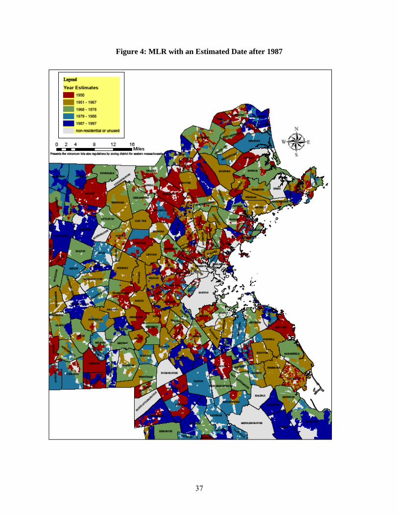
detail in Appendix 1. We estimate that there were 51 changes in MLR in zoning districts in 43

towns. We can see this spatially in Figure 4, where the dark blue zoning districts have passed a

regulation since 1987. The grey are either non-residential or are not used in the study because of

data issues.

To provide some information on whether these 45 towns are systematically different than the

remaining towns, we provide the means for observable characteristics across these two groups in

Table 3. First, contrary to expectations, towns with a change in MLR have lower house prices

23

compared to towns without a MLR change.6 Many of the other characteristics are significantly

different across the two groups. Clearly, we need to condition on these variables in the hedonic

regressions. This also raises the likelihood that these two groups of towns are different in other

unobservable ways. We deal with this problem by including zoning district fixed effects in the

regressions.

6. Results

We now present results from the hedonic regressions specified in Section 4. The main

variable of interest is MLR; the actual minimum lot size value in acres. This value is constant for

all zoning districts where no change took place. Recall that MassGIS only provides the minimum

lot size at a point in time without any prior regulatory information. Thus, for zoning districts where

we estimate a change in the minimum lot size took place, we assume that MLR is zero before the

change. This is an unrealistic assumption, but is necessary because of data limitations. This means

that our estimate of the impact of MLR on prices is a lower bound on the true regulatory price

effect. Further, the measurement error from having to estimate the changes in MLR will further

attenuate the estimates.

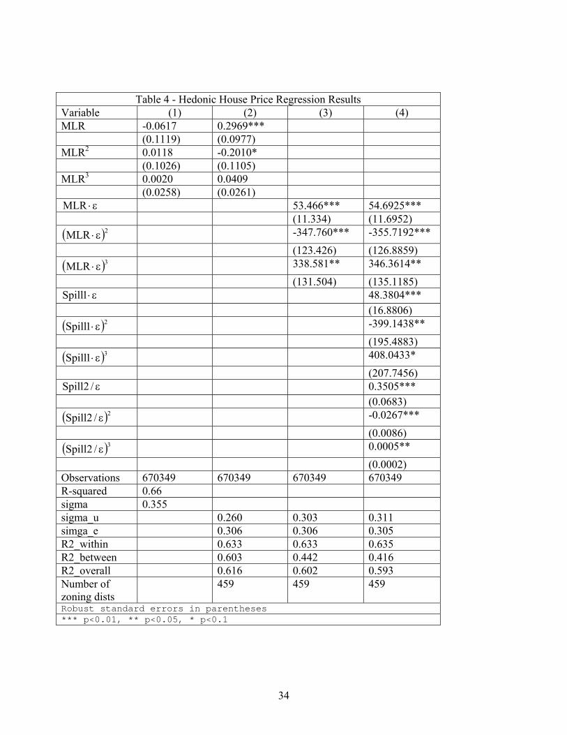
Given the nonlinear nature of the regulatory impact, we include MLR, its square and its cube

as regressors in the hedonic model. We first estimate the standard hedonic house price equation

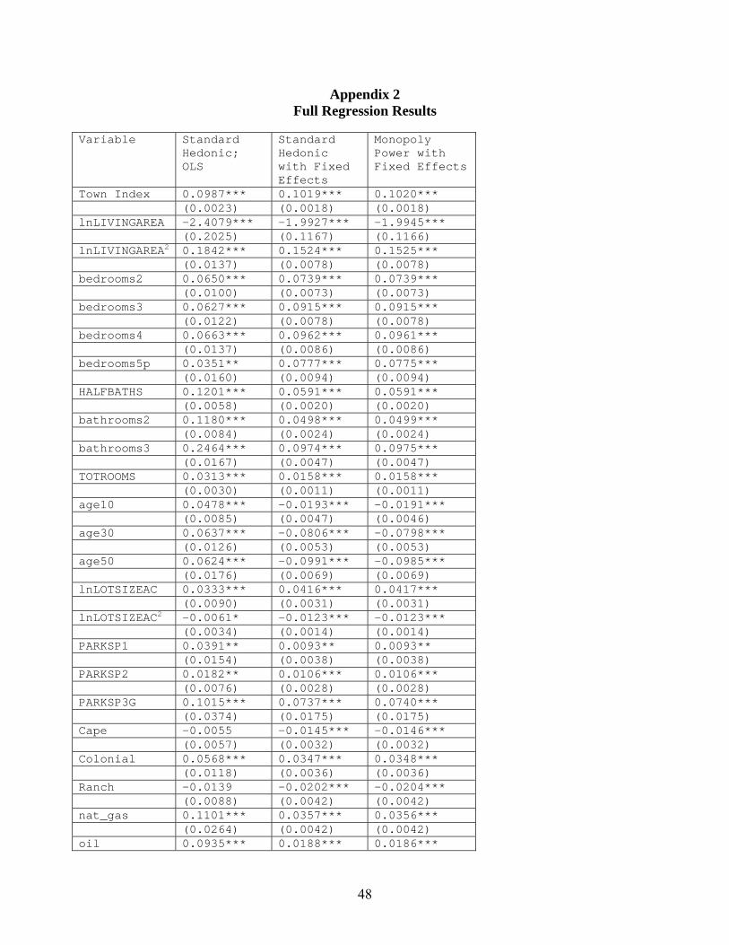
(equation 9) by OLS. The structural characteristics that we include are given in Table 1 (with the

exception that we include logs of living area and lot size and their squares). Column (1) of Table 3

provides estimates of the hedonic house price regression without fixed effects. The results for the

MLR variables are given in column (1) of Table 4. The full set of results is given in the Appendix

6 Pendall et al (2006) note that previous evidence clearly indicates that house prices are higher in more regulated jurisdictions. Of course, this could reflect the treatment (LURs) as well as initial section.

24

2. The p-value for the F-test for the joint significance of the three MLR variables is 0.458. So the

results from the standard model provide no evidence that an increase in MLR will affect house

prices. To see the impact of MLR on prices, we evaluate at all zoning districts within the 10th –

90th percentiles of the distribution of zoning district MLRs. We choose this range so as to exclude

the extreme values of the distribution, whose associated impacts are estimated with less confidence.

The impacts are presented in Figure 5. As one can see, these impacts are negative but fairly small

as indicated by the joint insignificance of the MLR coefficients.

Next we estimate the standard model including zoning district fixed effects. The results for

the MLR variables are given in column (2) of Table 4. These coefficients are now jointly

significant at the 1% level. The impacts for the MLRs in the 10th – 90th percentile range are also

given in Figure 4. Now we see a positive and economically significant impact of MLR; a 12-14%

effect in the range of values of MLR between 1 and 2 acres.

Recall that the impact of MLR will depend on the monopoly zoning power of the town, kε .

Our measure of monopoly zoning power for town k is the minimum of the absolute value of the

difference in town k’s fixed effect and that for all other towns (see equation 2). We estimate the

town fixed effects from a regression of the log of house price on structural characteristics, MLR,

year dummies, and town dummies. The coefficients on the town dummies are the town fixed

effects. Hence our regulatory variable is now kjktMLR ε⋅ .

Given the nonlinear nature of the regulatory impact, we include kjktMLR ε⋅ , its square, and its

cube as regressors in the hedonic model. The coefficients on the three MLR variables are jointly

significant at the 1% level. To see how the change in MLR affects house prices, we plot the

impacts for zoning districts that change their minimum lot size in Figure 4. Again, we include

impacts from distribution of values of the kjktMLR ε⋅ variable from the 10th to the 90th percentile.

25

Note that kjktMLR ε⋅ is multiplied by 175 so that the scale is similar to MLR. Clearly the towns

that have larger monopoly power show significantly larger price impacts with the largest being

around 24%. Thus accounting for monopoly power results in larger impacts; particularly in the

zoning districts with greater monopoly power.

Given that the full effect of a new land use regulation may occur over time, we are interested

in how the time since the regulation was passed affects the regulatory price effect. To do so, we

define new variables that capture the impacts in three-year intervals; 0-3, 3-6, 6-9, 9-12, and 12-15,

that measure years since the MLR changed. Again, since we include up to cubic terms, results are

best viewed in a graph; Figure 6 in this case. We see that the impact does increase over time. It

looks like the impacts between 3-6 and 6-9 years after the regulation are the same and greater than

the impact between 0-3 years and this is confirmed by an F-test. Further, it looks like the impacts

between 9-12 and 12-15 years after the regulation are the same and greater than the impacts

between 3-9 years and this is also confirmed by an F-test. This provides evidence that the impact

of a change in MLR takes time to reach its full effect and that these impacts can be quite substantial

10 – 15 years after the change.

Next we add the spillover variables to the model. To measure the intra-town spillover effects,

Spill1 equals MLRjkt for other zoning districts in town k when there is a change in one zoning

district in the town. One complication is that there are changes in MLR in multiple zoning districts

in seven towns. In two of these towns, the change occurred in the same year in two zoning

districts. In this case, in the other zoning districts, Spill1 is equal to the largest MLR change in the

two zoning districts that change MLR. Note that Spill1 is zero in the two zoning districts that

change MLR so the spillover effect is only measured in zoning districts that do not change MLR.

In one town there are only two zoning districts and both change MLR so we do not measure a

26

spillover effect in this town. In towns with zoning districts that change MLR in different years, we

measure the spilllover effect after the most recent change in MLR.

We measure the inter-town spillover effect in the nearest town. So assume that there is a

change in MLR in zoning district m in town n and town k is the closest town. Then for zoning

district j in town k, Spill2 equals the ratio of MLRmnt and MLRjkt for other zoning districts in town

k when there is a change in a zoning district in the closest town. Two complications arise in

constructing Spill2. First, as mentioned above, there can be a change in MLR in more than one

zoning district in a town. In this case, we measure Spill2 as the sum of the spillover effects from

the two zoning districts that changed MLR. A second complication is that a town can be the

recipient of spillover effects from more than one town. Again, we add the spillover effects when

generating Spill2. We include up to cubic terms in Spill1 and Spill2 as regressors. The results for

the spillover variables are given in column (4) of Table 4. Both sets of spillover variables are

jointly significant at the 1% level. Once again, it is best to see the impacts in a graph; Figure 7.

One can see that the regulatory impact is largest in the zoning district in which the MLR changed.

Impacts are smaller in other zoning districts in the same town and smaller still in nearby towns.

Still both the spillover effects are significant in both a statistical and an economic sense. We also

let the spillover impacts vary over time as we did for the own impacts but these results showed no

clear evidence of this.

While we include zoning district fixed effects and individual town price indices, there is some

potential for a positive bias if towns implement minimum lot size changes in response to rising

prices in the zoning district. To check for this, we re-estimated the model with linear trends in the

zoning district fixed effects. If anything, the impact is even stronger than when only zoning district

fixed effects are included. Hence, we do not see this scenario arising in our data.

27

Finally, as a robustness check, we allow for the change in MLR to affect prices prior to the

change. If this impact is significant, then one would be concerned that MLR change in correlated

with some other, unobserved, factor that affects house prices. Fortunately, this impact is small and

not significantly different from zero. This can be viewed as evidence in support of the causal

impact of MLR on house prices.

7. Conclusion

In this paper, we have provided clear evidence that land use restrictions (LURs) can

significantly impact house prices. In this case, we focus on a land use regulation that would appear

to have the most potential for price effects; minimum lot size restrictions (MLRs). We have

overcome a number of problems which makes previous estimates of the impact of LURs on house

prices less credible. First, we have controlled for the endogeneity of land use restrictions by

including zoning district fixed effects in our hedonic model. Further, we include town-level price

indices that minimize the bias that arise from towns implementing LURs when prices are rising (pr

falling). Second, we account for monopoly power; the town’s ability to sustain price increases.

Third, because we include zoning district fixed effects, identification of the impact of MLR on

house prices comes from changes in MLR. We have developed a detailed dataset over a reasonably

long time period that allows us to capture a significant number of changes in MLR.

Our results show that MLR does have an economically significant impact on house prices.

Further, we provide evidence that this impact increase over time. Finally, we find evidence of both

intra- town and inter-town spillover effects but these are not as large as those in the zoning districts

in which the MLRs change.

28

References Bai, Jushan, and Pierre Perron. 2003. Computation and analysis of multiple structural change models. Journal of Applied Econometrics 18(1):1. Case, Karl E., and Christopher J. Mayer. 1995. Housing price dynamics within a metropolitan area. Federal Reserve Bank of Boston. Cho, M and P. Linneman. 1993. Interjurisdictional Spillover Effects and Land Use Restrictions. Journal of Housing Research 4(1): 131-163. Ellickson, RC. 1977. Suburban Growth Controls- Economic and Legal Analysis. Yale Law Journal 86(3):385-511. Fischel, William A. 2001. The Homevoter Hypothesis: How Home Values Influence Local Government Taxation, School Finance, and Land-Use Policies. Cambridge, Mass: Harvard University Press. Glaeser, E. L., and Joseph Gyourko. 2002. The Impact of Zoning on Housing Affordability. NBER Working Paper 8835. Glaeser, Edward L., and Bryce A. Ward. 2006. The Causes and Consequences of Land Use Regulation: Evidence from Greater Boston. NBER Working Paper 12601 Glickfield, M. and N. Levine. 1992. Regional Growth … Local Reaction: The Enactment and Effects of Local Growth Control and Management Measures in California. Lincoln Land Institute. Green, Richard K. 1999. Land Use Regulation and the Price of Housing in a Suburban Wisconsin County. Journal of Housing Economics 8: 144-159. Hamilton, Bruce W. 1978. Zoning and the exercise of monopoly power. Journal of Urban Economics 5, no. 1:116-130. Hamilton, BW. 1975. Zoning and Property Taxation in a System of Local Governments. Urban Studies 12, no. 2:205-211. Ihlanfeldt, K.R. 2004. Introduction: Exclusionary land-use regulations. Urban Studies 41(2). 2: 255-259. Ihlanfeldt, K.R. 2007. The effect of land use regulation on housing and land prices. Journal of Urban Economics 61(3): 420-435. Katz, L., and Kenneth Rosen. 1987. The Interjurisdictional Effects of Growth Controls on Housing Prices. Journal of Law & Economics 30(1): 149-60.

29

Knapp, Gerrit-Jan, Yan Song, and Zorica Nedovic-Budie. 2007. Measuring Patterns of Urban Development: New Intelligence for the War on Sprawl. Local Environment 12(3): 239-257. Kopitz, Elizabeth, Virginia McConnell, and Daniel Miles. 2007. Lot Size, Zoning, and Household Preferences: Impediments to Smart Growth? Conference paper 08, Smart Growth @ 10 Conference. Landis, J.D. 1992. Do Growth Controls Work? A New Assessment. Journal of the American Planning Association 30: 149-160. Levine, N. 1999. The Effects of Local Growth Controls on Regional Housing Production and Population Redistribution in California. Urban Studies 30: 2047-2068. Malpezzi, Stephen. 1996. Housing Prices, Externalities, and Regulation in US Metropolitan Areas. Journal of Housing Research 7(2): 209-241. Pendall , Rolf, Robert Puentes, and Jonathan Martin. 2006. From Traditional to Reformed: A Review of the Land Use Regulations in the Nation’s 50 Largest Metropolitan Areas. Research Brief, Metropolitan Policy Program, The Brookings Institution. Pogodzinski, J.M., and Tim R. Sass. 1991. Measuring the Effects of Municipal Zoning Regulations: A Survey. Urban Stud 28(4): 597-621. Pollakowski, HO, and SM Wachter. 1990. The Effect of Land-Use Constraints on Housing Prices. Land Economics 66(3): 315-324. Quigley, J. and S. Raphael. 2004. Regulation and the High Cost of Housing in California. American Economic Review, 94(2), 2005: 323-329. Quigley, John, and Larry Rosenthal. 2005. The Effects of Land-Use Regulation on the Price of Housing: What Do We Know? What Can We Learn? Cityscape 8(1): 69-137. Rosen, S. 1974. Hedonic Prices and Implicit Markets: Product Differentiation in Pure Competition. Journal of Political Economy 82(1): 34-55. Thorson, J.A. 1997. The Effect of Zoning on House Construction. Journal of Housing Economics 6(1): 81-91. Tiebout, CM. 1956. A Pure Theory of Local Expenditures. Journal of Political Economy 64(5): 416-424. Zeileis, Achim, Christian Kleiber, Walter Kramer, and Kurt Hornik. 2003. Testing and dating of structural changes in practice. Computational Statistics & Data Analysis 44, no. 1-2:109-123.

30

Table 1 – Summary Statistics

Variable Mean Std Dev Min Max

Nominal House Price (in $1,000s) 302.73 233.42 20 5,000 Real House Price ($2006) 493.55 323.46 19.42 12,563.53 Living Area (sq ft) 1927.11 877.47 88 20,043 Total Number of Rooms 6.95 1.62 3 23 2 Bedrooms 0.12 0.32 0 1 3 Bedrooms 0.52 0.50 0 1 4 Bedrooms 0.30 0.46 0 1 5 or more Bedrooms 0.06 0.23 0 1 2 Bathrooms 0.43 0.50 0 1 3 or more Bathrooms 0.10 0.30 0 1 Number of Half Bathrooms 0.59 0.54 0 6 10 <= House Age <= 30 0.20 0.40 0 1 10 < House Age <= 50 0.26 0.44 0 1 50 < House Age 0.35 0.48 0 1 Lot Size (Acres) 0.62 0.80 0.01 10 1 Parking Space 0.13 0.34 0 1 2 Parking Spaces 0.21 0.61 0 2 3 or more Parking Spaces 0.01 0.09 0 1 Cape = 1 0.14 0.35 0 1 Colonial = 1 0.32 0.47 0 1 Ranch = 1 0.16 0.36 0 1 Natural Gas Heat = 1 0.41 0.49 0 1 Oil Heat = 1 0.51 0.50 0 1 Basement Finished Area 3.77 5.16 0 51.57 1 Fireplace 0.45 0.50 0 1 2 or more Fireplaces 0.12 0.33 0 1 Poor Condition 0.01 0.07 0 1 Town Index

31

Table 2 – Lot Sizes for New Houses; 1950 - 2005

Year Built Number Mean Lot Size Median Lot Size

1950 11792 0.38 0.241951 3429 0.41 0.251952 4866 0.40 0.261953 4457 0.39 0.261954 4702 0.43 0.281955 9010 0.42 0.291956 4884 0.46 0.311957 4314 0.48 0.331958 4244 0.50 0.351959 3564 0.54 0.381960 10171 0.47 0.341961 3532 0.58 0.411962 4474 0.56 0.411963 4016 0.58 0.421964 4124 0.60 0.441965 5485 0.59 0.431966 3841 0.65 0.471967 3364 0.69 0.491968 4096 0.71 0.51969 3357 0.76 0.561970 4471 0.71 0.491971 3053 0.75 0.521972 4070 0.78 0.561973 3514 0.80 0.571974 2844 0.84 0.61975 2722 0.85 0.591976 2826 0.90 0.61977 2833 0.97 0.711978 3247 1.00 0.711979 2827 1.02 0.741980 2495 1.05 0.691981 2029 1.09 0.751982 1855 1.01 0.691983 3178 1.03 0.731984 3873 1.10 0.781985 4794 1.07 0.731986 5370 1.07 0.751987 6115 0.96 0.691988 5023 0.96 0.691989 4379 0.93 0.671990 3539 0.95 0.69

32

1991 3534 1.00 0.751992 5193 1.04 0.81993 5520 1.07 0.841994 5819 1.03 0.751995 5009 1.03 0.731996 5314 1.06 0.741997 5442 1.07 0.771998 5601 1.06 0.741999 4892 1.09 0.742000 3747 1.16 0.92001 2591 1.10 0.792002 2487 1.05 0.652003 2006 1.01 0.622004 2175 0.96 0.552005 1524 0.88 0.46

33

Table 3 – Comparison of Means for Towns With and Without Change in MLR

Variable

Mean for Towns w/o change in MLR

Mean for Towns with change in MLR

p-value for equality of Means

House Price (in $1,000s) 214.93 188.76 0.00 (125.62) (115.47) Living Area (sq ft) 1,920.76 1,818.29 0.00 (796.77) (773.47) Total Number of Rooms 7.06 6.72 0.00 (1.57) (1.45) Number of Bedrooms 3.32 3.23 0.00 (0.81) (0.77) Number of Half Bathrooms 0.59 0.53 0.00 (0.54) (0.53) Number of Bathrooms 1.66 1.57 0.00 (0.70) (0.67) House Age 36.68 33.06 0.00 (33.22) (30.75) Lot Size (acres) 0.59 0.51 0.00 (0.73) (0.60) Number of Parking Spaces 0.37 0.39 0.03 (0.70) (0.69) Cape = 1 0.14 0.13 0.03 (0.35) (0.34) Colonial = 1 0.30 0.27 0.00 (0.46) (0.44) Ranch = 1 0.15 0.19 0.00 (0.36) (0.39) Natural Gas Heat = 1 0.40 0.44 0.00 (0.49) (0.50) Oil Heat = 1 0.52 0.51 0.17 (0.50) (0.50) Basement Finished Area 3.98 3.48 0.00 (5.19) (4.62) Number of Fireplaces 0.80 0.71 0.00 (0.81) (0.75) Poor Condition 0.008 0.001 0.00 (0.09) (0.04) Minimum Lot Size 0.78 0.79 0.90 (0.53) (0.66)

34

Table 4 - Hedonic House Price Regression Results Variable (1) (2) (3) (4) MLR -0.0617 0.2969*** (0.1119) (0.0977) MLR2 0.0118 -0.2010* (0.1026) (0.1105) MLR3 0.0020 0.0409 (0.0258) (0.0261)

ε⋅MLR 53.466*** 54.6925*** (11.334) (11.6952) ( )2MLR ε⋅ -347.760*** -355.7192*** (123.426) (126.8859) ( )3MLR ε⋅ 338.581** 346.3614** (131.504) (135.1185)

ε⋅1Spill 48.3804*** (16.8806) ( )21Spill ε⋅ -399.1438** (195.4883) ( )31Spill ε⋅ 408.0433* (207.7456)

ε/2Spill 0.3505*** (0.0683) ( )2/2Spill ε -0.0267*** (0.0086) ( )3/2Spill ε 0.0005** (0.0002) Observations 670349 670349 670349 670349 R-squared 0.66 sigma 0.355 sigma_u 0.260 0.303 0.311 simga_e 0.306 0.306 0.305 R2_within 0.633 0.633 0.635 R2_between 0.603 0.442 0.416 R2_overall 0.616 0.602 0.593 Number of zoning dists

459 459 459

Robust standard errors in parentheses *** p<0.01, ** p<0.05, * p<0.1

35

.2.4

.6.8

1M

edia

n Lo

t Siz

e

1950 1955 1960 1965 1970 1975 1980 1985 1990 1995 2000 2005Year Built

Figure1Median Lot Size for New Houses, 1950-2005

0.0

5.1

.15

.2.2

5Fr

actio

n

0 1 2 3 4 5Minimum Lot Size

Figure 2Distribution of Minimum Lot Sizes in Zoning Districts

36

Figure 3: Zoning Districts Used with MLR of .9 or Greater

37

Figure 4: MLR with an Estimated Date after 1987

38

-10

010

2030

Per

cent

Impa

ct

0 .5 1 1.5 2MLR/MLR*Monopoly Power*175

OLS Zoning District Fixed EffectsIncludes Monopoly Power

Figure 5:Percent Impact of Minimum Lot Size Change on Price

010

2030

40P

erce

nt Im

pact

0 .002 .004 .006 .008MLR*Monopoly Power

0-3 years 3-6 years6-9 years 9-12 years12-15 years

Figure 6:Time Varying Impacts

39

020

4060

Perc

ent I

mpa

ct

0 .002 .004 .006 .008MLR*Monopoly Power

-3-0 years 0-3 years3-6 years 6-9 years9-12 years 12-15 years

Figure 6:Time Varying Impacts

05

1015

2025

Per

cent

Impa

ct

0 .002 .004 .006 .008 .01MLR*Monopoly Power

Zone Impact Other Zones in Same TownNearby Town

Figure 7:Spillover Effects

40

Appendix 1 Estimating the Minimum Lot Size Change Date

One problem with the regulation data used in this study is that the date the MLR was passed

is not available from MassGIS’s MLR database. We need these dates to able to implement our procedure for estimating the regulatory price effect. In order to overcome this data deficiency, the date at which the regulations were passed is estimated through the use of an endogenous structural dating procedure.

Descriptions of MassGIS Data and Zoning level Lot size Time Series One of the data sources used for estimating the date MLRs are passed comes from a fairly

recent study by MassGIS which documents and identifies the MLR and zoning districts for all of Massachusetts for a single point in time. For eastern Massachusetts, the data set is mostly based on data current as of 2000, with a few exceptions dating back to 19907 . As noted above, this data only gives MLR for a single point in time and is the reason why these dates need to be estimated.

The data is found on the MassGIS Zoning layer8 website and provides the boundaries of municipal zoning districts in an ARCgis shape file and a table linking the zoning districts to the minimum lot size. A slight complication occurs in identifying zoning district level minimum lot size because each zoning district is able to assign minimum lot sizes to different uses. As a result, the median MLR is used as the MLR because only a small percentage of the zoning districts report more then one minimum lot size. However this does not affect the regulatory measure much9 and only slightly changes our interpretation of the regulatory measure as a median level of stringency. The zoning data includes information on non-residential zoning but we limit ourselves to residential zoning using the general zoning categories MassGIS provides in the data set. In total there are 669 residential zoning districts10 in eastern Massachusetts.

An additional data source used to create the time series of lot sizes is from the Warren Group. It provides information on zoning districts, addresses, lot sizes (acres) and the date when the house was built. These variables are used to create a time series of lot sizes, where the time is indexed by the year a house was built. Note that zoning information from the Warren group is not available for all cities and is why MassGIS zoning boundaries are used for all of the observations.

In order to use the full sample of eastern Massachusetts towns, the Warren Group parcel level data is geo-coded using ARCgis11 and combined with the zoning district boundaries from MassGIS using the spatial join feature in ARCgis. This procedure allows us to identify which zoning district the Warren Group parcel level data fall within. The spatial join using the MassGIS zoning boundaries is necessary because the Warren Group does not provide zoning data for all of the cities. The Warren Group zoning information will be used to test the accuracy of the MassGIS boundaries.

Once the Warren Group data has been grouped into zoning districts, the lot size and year built variable from the Warren Group is used to create a time series of a summary measure of zoning 7 See http://www.mass.gov/mgis/st_zn.jpg for a comprehensive map 8 Available at http://www.mass.gov/mgis/zn.htmA difficulty with the zoning data is that MLRs can differ by use within each zoning district. 9 Using the median minimum lot size within each zoning district results in less then 1% of the minimum lot size levels calculated in each zone to be larger then the actual minimum lot size by a margin greater then .1 acre. 10 In addition 33 zoning districts either have no reference to minimum lot sizes or use a formula to calculate it. These are excluded from the study. 11 The maps used to geocode the data are from ESRI with the help of the MIT GIS Lab

41

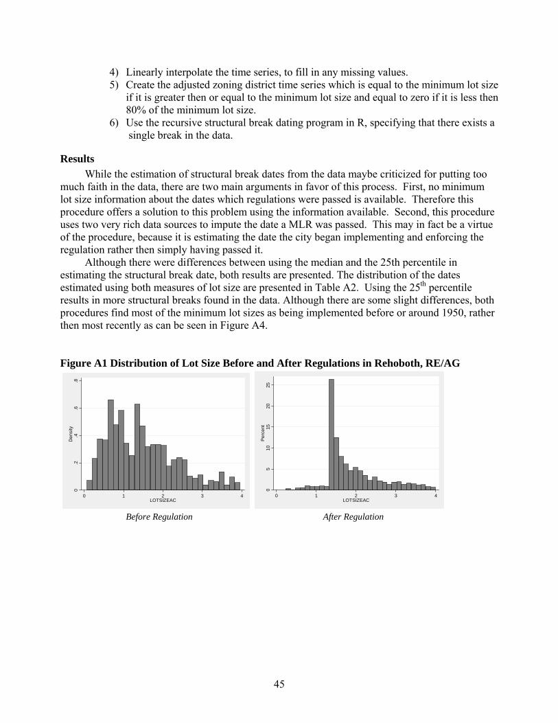
level lot sizes within each year. Choosing the correct summary level lot size measure within each zoning district is important because it has implications for the identification of the date regulations were passed. At first, it may seem natural to use the median lot size for each zoning district by year built. However, this may not properly capture the true change in lot sizes caused by a MLR. For example, suppose we are concerned with a single zoning district which passes a MLR of 0.5 acres in 1960. Before the regulation was passed assume that the natural minimum lot size set by the market in the district was 0.1 acres. In one instance, we can imagine that the implementation of the MLR causes a shift of the entire lot size distribution to the right, resulting in a change of the median lot size. A more reasonable assumption is that the distribution may not shift at all, instead all of the houses built at the natural minimum lot size of 0.1 acres will simply be forced to build on 0.5 acre plots and the remainder of the distribution will stay the same. The median lot size may not be affected by this type of a change in the distribution if the regulation is less then the median lot size for the time series. Figure A1 provides an example from the data set of how the lot size distribution changes with a MLR, using the estimated break dates from this section. From Figure A1, it seems that that much of the building occurs at the MLR lot size. It turns out that the choice between using the median or the 25th percentile is arbitrary. We decide to use the 25th percentile (p25) because it should be able to capture a little bit of both types of distribution shifts.12

Having decided on using the 25th percentile, a time series of lot sizes using MassGIS boundary data is constructed from the Warren Group data. The time is indexed by the year built variable going back to 1950. The resulting time series does not encompass all of the zoning districts MassGIS identifies in eastern Massachusetts. In particular, the number of zones drops down to 620 from a total of 669 because we limit our dataset to housing records built after 1949. An additional restriction used is to only use zones which contain thirty or more observations for the 1950 to 2004 time period. This ensures that we have enough data within each zoning district to estimate the structural break. The result is that we end up using 474 zoning districts in eastern Massachusetts. Finally, the data is also linearly interpolated to account for any missing values in the time series.

The195 zoning districts dropped are from 81 cities. For the majority of cities, 49 of the 81, we are dropping a single zoning district from each town. The dropped zoning districts had some of the largest MLRs in eastern Massachusetts; including those of 8 and 10 acres. However these zoning district were small relative to the districts used. The 195 dropped zoning districts only make up 6.6% of all the residential zoned areas in eastern Massachusetts, suggesting that the zoning districts dropped do not make up a large amount of the housing stock.

A potential drawback of relying on the MassGIS boundary file to identify the zoning districts each town lies within is the questionable accuracy of the zoning boundary file. Closer inspection of the shape file shows that although the zoning boundaries are located within or along town boundaries, some of the boundaries lie between major roadways; which is counterintuitive to where we expect zoning boundaries to lie. As a result, the next section uses the zoning information in the

12 A simple solution to see which of these better describes how the distribution of lot size changes in response to a regulation is to use a different measure. We maybe tempted to simply report the minimum lot size in each zoning period, however the lot size variable has some errors due to exclusions from the regulations and potential reporting inaccuracies. A better measure could be to use some other percentile to capture the affect of regulation on the zoning districts lot size. The lot size time series are created using the median and the 25th percentile lot size within each year. The difference in the estimated years the MLRs passed are reported. Note that for zoning boundaries defined by the Warren Group and those defined using the MassGIS zoning boundaries, about 50 percent of the dates remain nearly the same resulting in a change of plus or minus 1 year. Perhaps more disconcerting is that changing the lot size measure from the median lot size to the 25th percentile changes 20 percent of the date plus or minus 15 years in both samples. Both of these dates are used in the panel regression run in the last section and we find no significant difference between the two measures. This leads us to believe that the choice between the two is arbitrary.

42

Warren Group data for a group of cities in order to determine the amount of measurement error in our estimates.

Testing the Validity of MassGIS Data In order to ensure the accuracy of the zoning boundaries reported by MassGIS, the 25th

percentile (p25) lot size time series constructed from Warren Group zoning data13 and MassGIS boundary files are compared. The Warren Group reports the correct zoning district since it is from the assessors’ files and provides a useful comparison to test the accuracy of MassGIS zoning boundaries. The Warren Group zoning data with the corrected zoning codes is used to group parcels into the zoning districts which are reported in the MassGIS MLR data.

The Warren Group data does not provide zoning information for all households in all cities. It provides zoning information for 96 of the 187 cities used in this study, consisting of around one third of all observations. All of the zoning codes the Warren Group reports do not necessarily match the residential zoning boundary codes reported in the MassGIS zoning data. The total matched regulations make up 36% of the total sample. In addition to losing observations because zoning district codes in the Warren Group and MassGIS do not match, some zoning districts are not used because an insufficient amount of data lies within them to create a complete time series.

The time series of lot sizes within city zoning districts is constructed using the Warren Group and MassGIS zoning information separately. Then the datasets are combined for comparison purposes. Of the total 155 zoning districts used for the comparison, 34 zoning districts report a different estimated structural break date. The difference in the estimated structural break date due to minor error, defined as plus or minus 13 years, occurs for 18 of the 34 changed zoning areas. Another 5 zoning areas have a year error of between plus or minus 40. The remaining 11 of 34 zoning areas experienced major errors due to the methodology incorrectly identifying whether a zone experienced a structural break or not.

A similar comparison of the p25 lot sizes for the two zoning district time series provides a finer measure of the amount of error which maybe occurring. Summary statistics for the median lot size are reported in Table A1. The mean p25 lot size difference for all zoning areas is -.01. This indicates that the median lot size for a zoning area using Warren Group zoning data is on average smaller then the zoning districts median lot sizes constructed by using MassGIS zoning boundaries. Overall the difference in lot sizes is not large, and more emphasis is placed on the differences between the estimated structural break dates.

This simple analysis confirms that the MassGIS zoning map layers in ARCgis are not entirely accurate. However what this analysis suggests is that the degree of accuracy is somewhat palatable. Using the error rates from the dating of structural breaks in the Warren Group zoning sample, we next apply these error rates to the 474 zoning areas used with the MassGIS boundary data. These error rates predict that 55 of the 474 zones will miss the actual structural break date by plus or minus thirteen years. The more problematic error of incorrectly identifying the structural date will occur 7.1% of the time or for about 33 zones. All together we can expect to miss the correct structural break date due to the inaccuracy of the MassGIS zoning maps around 22% of the

13 One problem found with the Warren Group zoning variable was that the zoning information in many cases didn’t exactly match the MassGIS data, but was fairly close. For example the zoning code could be reported in all capital letters in one data source and lowercase letters in the other. Other examples are due to mismatching hyphens and abbreviations in the data sources. These records were corrected by hand by comparing all of the potential zoning codes within cities for both Warren Group and MassGIS zoning data

43

time. We do not believe this amount of error to be significant, although it may introduce some bias14into our estimates.

To get a better idea of the data constructed, two brief examples are presented. Graph 2 and 3 plot p25 lot size time series for two zoning districts going back in time, by year the house was built, to 1900 although we only use data since 1950 to estimate the structural break. The vertical line is the estimated date which MLR were passed, the “x” are time series for this zoning district from MassGIS zoning boundaries and the “o” are the one based on the Warren Group Zoning information.

Estimation of the Structural Break Date Once the time series is properly constructed from the Warren Group lot size and year built

variables for each zoning district, the estimation of the structural date can proceed. Since the purpose is to estimate the date which MLRs were passed, the time series are modified to incorporate the actual minimum lot size information MassGIS provides. This is done by creating a new time series for which the lot size is equal to the minimum lot size if the p25 lot size for that specific year is greater then the minimum lot size. If the median lot size is less then 80% of the minimum lot size then the median lot size is set equal to zero. The reasoning for making these changes is to ensure that the structural breaks estimated are relevant to the MLRs passed and not some other factor affecting lot size.

An example of the changes made to the time series is presented in Figure A4. Note that the “x”’s are the p25 lot size within Newbury’s “R/A” zoning district taken from the Warren Group data using the MassGIS zoning boundaries. The dashed horizontal line is the minimum lot size reported by MassGIS and the vertical line is the estimated break date. The “o”s are the adjusted time series, which sets the value equal to the minimum lot size if the median lot size is greater then the reported minimum lot size and equal to zero if its median lot size is less then 80% of the reported minimum lot size. Note that this enables the procedure to better capture structural breaks occurring around the minimum lot size.

Once the time series are adjusted to account for the MLR, the structural breaks are estimated using an endogenous structural break dating procedure. The following closely follows the framework presented in Zeileis, Kleiber, Kramer, and Hornik (2003) and deals with the following regression model for a single zoning district within a city in our case.

tjt uXL += β where Lt is the p25 adjusted lot size in the tth time period, X is a data matrix of controls including a column of 1s, and jβ is a vector of coefficients which may vary over time. Assuming that the model in question has m structural breaks, the data can be thought of being partitioned into m+1 segments which are indexed by j . While this framework allows for controls, the following analysis includes a constant in the regression. As a result, the estimation of a structural break is with respect to a shift in the 25th percentile (p25) zoning district lot size for single family homes over time.

Under this framework the regression coefficients determines a structural break if they change over time periods. This amounts to testing the following hypothesis

,...,m3,2,1 j :H j == οο ββ

14 In the regression setting used in the final section of the empirical section, the measurement error could potentially cause attenuation bias. However we check for this by estimating the regulatory price effect for the same subgroup using different zoning boundaries and find no difference.

44

:aH One coefficient varies of time Carrying out the hypothesis test can be done using either an F-test or a generalized fluctuation test (GFT). The GFT captures the variability in the median lot size using the residuals or parameter estimates. Using these estimates, the test determines whether the deviations fall outsides of bounds found from functional central limit theorems (Zeileis, Kleiber, Kramer, and Hornik (2003)).

The literature recommends testing for the existence of a structural break using a GFT or F-test. The reason is, as Bai and Perron (2003) note, that in the presence of multiple structural breaks the following procedure may favor rejecting the zero versus one break and multiple breaks versus zero break hypotheses. The tests for the existence of a structural break are not used because we are only searching for a single break in these adjusted time series. Additionally, when the tests were used they resulted in the rejection of several break dates, when a structural break was present. For example, in Figures 2 and 3, the GFT test rejected the existence of a structural break, although a structural break occurred and was estimated, denoted by the vertical line.

The estimated date of the structural change is computed using the following procedure.

First, let RSS(i1,…,m)=∑+

=

+1m

1j1-j )i1,rss(i

jwhere )i1,rss(i j1-j + is the residual sum of squares for the

jth partition. The problem of dating the structural break is one of finding the partition ),..,( **1 mii such

that { })i,...,RSS(iargmin)i,..,(i m1

)mi,...,1(i

*m

*1 =

The optimization problem is solved recursively using Bellman’s principle, which involves a trimming parameter h that defines the minimum length which a break is searched within (Zeileis, Kleiber, Kramer, and Hornik (2003)). To see this note that the recursive optimization technique is solving the following equation where mn,γ denotes the partition from n to m

{ }n)1,rss(i-)RSS(γmin)RSS(γ j1,mhnnihmn

ji, += −−≤≤

Also note that nh = n*h and is where the parameter h gets its interpretation. The trimming parameter is set equal to .2 in the estimates presented below.

These tests are conveniently carried out in the R statistical programming language using a user defined program which is discussed in Zeileis, Kleiber, Kramer, and Hornik (2003) . The structural break dates can be estimated by specifying the number of breaks a priori or by using the Bayesian information criterion (BIC). The BIC is a function of the fit of the model, the number of parameters and sample size. Ward (2008) makes note that the BIC is increasing in both parameters and the fit of the model, indicating that lower BIC values correspond to a better model. Although we could argue that more then one break may occur because of more then one change in regulations, the procedure is set to look for a single break because the procedure is not capable of consistently estimating structural break with respect to a regulation without knowing what the previous regulation was.

The structural break estimation procedure is defined by the following steps 1) Use Warren Group and MassGIS zoning data to group the Warren Group parcel

level observation into a zoning district. 2) Create a time series of lot sizes from the Warren Group parcel data for each zoning

district using the 25th percentile lot size. 3) Trim the time series to only include households built after 1950 and zoning district

with enough observation to create a complete time series.

45

4) Linearly interpolate the time series, to fill in any missing values. 5) Create the adjusted zoning district time series which is equal to the minimum lot size

if it is greater then or equal to the minimum lot size and equal to zero if it is less then 80% of the minimum lot size.

6) Use the recursive structural break dating program in R, specifying that there exists a single break in the data.

Results While the estimation of structural break dates from the data maybe criticized for putting too

much faith in the data, there are two main arguments in favor of this process. First, no minimum lot size information about the dates which regulations were passed is available. Therefore this procedure offers a solution to this problem using the information available. Second, this procedure uses two very rich data sources to impute the date a MLR was passed. This may in fact be a virtue of the procedure, because it is estimating the date the city began implementing and enforcing the regulation rather then simply having passed it.

Although there were differences between using the median and the 25th percentile in estimating the structural break date, both results are presented. The distribution of the dates estimated using both measures of lot size are presented in Table A2. Using the 25th percentile results in more structural breaks found in the data. Although there are some slight differences, both procedures find most of the minimum lot sizes as being implemented before or around 1950, rather then most recently as can be seen in Figure A4. Figure A1 Distribution of Lot Size Before and After Regulations in Rehoboth, RE/AG

0.2

.4.6

.8D

ensi

ty

0 1 2 3 4LOTSIZEAC

05

1015

2025

Per

cent

0 1 2 3 4LOTSIZEAC

Before Regulation After Regulation

46

Figure A2 Median Lot Size within Holbrook’s “R3” Zoning District

Figure A3 Median Lot Size within Leicester’s “SA” Zoning District

0

1

2

3

4

Acres

1900 1920 1940 1960 1980 2000 year built

WG lot size minimum lot sizeMassGIS lot size

0

.5

1

1.5

2

Acres

1900 1920 1940 1960 1980 2000 Year built

WG lot size minimum lot sizeMassGIS lot size

47

Graph 4 p25 Lot Sizes within one of Newbury's R/A Zoning District

0.2

.4.6

.81

acre

s

1950 1960 1970 1980 1990 2000year built

p25 lot size adjusted lot sizeminimum lot size

Table A1 Summary Lot size(acre) Statistics

Median Mean Std. Dev. Min Max MassGIS MLR district lot size 0.40 0.76 1.52 0.03 77.00WG MLR district lot size 0.40 0.76 1.55 0.00 77.00difference(WG- MassGIS) 0.00 -0.01 0.70 -21.51 14.83This table is based on the comparison of Warren Group(WG) and MassGIS zoning data

Table A2 Difference in Estimated Year from using median versus 25th percentile MassGIS Zoning Data Warren Group Zoning

relative

frequency cumulative frequency

relative frequency

cumulative frequency

25 to 50 years 8.80 100.00 7.64 100.0025 year 6.76 91.20 7.78 92.3615 year 7.21 84.44 5.19 84.5810 year 12.29 77.23 14.86 79.395 year 19.52 64.94 15.50 64.531 year 45.42 45.42 49.03 49.03

48

Appendix 2 Full Regression Results

Variable Standard

Hedonic; OLS

Standard Hedonic with Fixed Effects

Monopoly Power with Fixed Effects

Town Index 0.0987*** 0.1019*** 0.1020*** (0.0023) (0.0018) (0.0018) lnLIVINGAREA -2.4079*** -1.9927*** -1.9945*** (0.2025) (0.1167) (0.1166) lnLIVINGAREA2 0.1842*** 0.1524*** 0.1525*** (0.0137) (0.0078) (0.0078) bedrooms2 0.0650*** 0.0739*** 0.0739*** (0.0100) (0.0073) (0.0073) bedrooms3 0.0627*** 0.0915*** 0.0915*** (0.0122) (0.0078) (0.0078) bedrooms4 0.0663*** 0.0962*** 0.0961*** (0.0137) (0.0086) (0.0086) bedrooms5p 0.0351** 0.0777*** 0.0775*** (0.0160) (0.0094) (0.0094) HALFBATHS 0.1201*** 0.0591*** 0.0591*** (0.0058) (0.0020) (0.0020) bathrooms2 0.1180*** 0.0498*** 0.0499*** (0.0084) (0.0024) (0.0024) bathrooms3 0.2464*** 0.0974*** 0.0975*** (0.0167) (0.0047) (0.0047) TOTROOMS 0.0313*** 0.0158*** 0.0158*** (0.0030) (0.0011) (0.0011) age10 0.0478*** -0.0193*** -0.0191*** (0.0085) (0.0047) (0.0046) age30 0.0637*** -0.0806*** -0.0798*** (0.0126) (0.0053) (0.0053) age50 0.0624*** -0.0991*** -0.0985*** (0.0176) (0.0069) (0.0069) lnLOTSIZEAC 0.0333*** 0.0416*** 0.0417*** (0.0090) (0.0031) (0.0031) lnLOTSIZEAC2 -0.0061* -0.0123*** -0.0123*** (0.0034) (0.0014) (0.0014) PARKSP1 0.0391** 0.0093** 0.0093** (0.0154) (0.0038) (0.0038) PARKSP2 0.0182** 0.0106*** 0.0106*** (0.0076) (0.0028) (0.0028) PARKSP3G 0.1015*** 0.0737*** 0.0740*** (0.0374) (0.0175) (0.0175) Cape -0.0055 -0.0145*** -0.0146*** (0.0057) (0.0032) (0.0032) Colonial 0.0568*** 0.0347*** 0.0348*** (0.0118) (0.0036) (0.0036) Ranch -0.0139 -0.0202*** -0.0204*** (0.0088) (0.0042) (0.0042) nat_gas 0.1101*** 0.0357*** 0.0356*** (0.0264) (0.0042) (0.0042) oil 0.0935*** 0.0188*** 0.0186***

49

(0.0264) (0.0037) (0.0037) BASMUFAREA -0.0006 0.0045*** 0.0045*** (0.0019) (0.0004) (0.0004) FIREPL1 0.1003*** 0.0665*** 0.0664*** (0.0126) (0.0029) (0.0029) FIREPL2 0.2234*** 0.1166*** 0.1165*** (0.0164) (0.0045) (0.0045) Poor -0.0058 -0.2041*** -0.2042*** (0.0851) (0.0201) (0.0201) MLR -0.0617 0.2969***

(0.1119) (0.0977)

MLR2 0.0118 -0.2010*

(0.1026) (0.1105)

MLR3 0.0020 0.0409

(0.0258) (0.0261)

ε⋅MLR 53.4663***

(11.3340)

( )2MLR ε⋅ -347.7601***

(123.4263)

( )3MLR ε⋅ 338.5809**

(131.5035) Observations 670349 670349 670349 R-squared 0.66 Sigma 0.355 sigma_u 0.260 0.303 simga_e 0.306 0.306 R2_within 0.633 0.633 R2_between 0.603 0.442 R2_overall 0.616 0.602 Number of zoning dists

459 459