The iterative complex demodulation applied on short and ...

Contributions to Geophysics and Geodesy Vol. 44/4, 2014 (313–328)

The iterative complex demodulationapplied on short and long Schumannresonance measured sequences

Adriena ONDRASKOVA, Sebastian SEVCIK

Department of Astronomy, Physics of the Earth and MeteorologyFaculty of Mathematics, Physics and InformaticsComenius University Mlynska dolina F-1, 842 48 Bratislava, Slovak Republic;e-mail: [email protected], [email protected]

Abstract: The precise determination of instantaneous frequency of Schumann resonance

(SR) modes, with the possibility of application to relatively short signal sequences, seems

to be important for detailed analysis of SR modal frequency variations. Contrary to com-

monly used method of obtaining modal frequencies by the Lorentz function fitting of DFT

spectra, we employ the complex demodulation (CD) method in iterated form. Results of

iterated CD method applied on short and long measured sequences are compared. Re-

sults for SR signals as well as the comparison with Lorentz function fitting are presented.

Decrease of frequencies of all first four SR modes from the solar cycle maximum to solar

cycle minimum has been found using also the CD method.

Key words: Schumann resonances, complex demodulation, instantaneous frequency

1. Introduction

The well-known phenomenon of Schumann resonances (SR) has been a sub-ject of monitoring at many observatories around the world. For extractingof quantitative information buried in the measured and recorded raw data,it is necessary to apply a suitable method of spectral (frequency) analysis.

The determination of instantaneous (short-term) modal frequencies fromsample sequences of non-stationary signal consisting of several damped har-monic components (modes), plus wideband noise and hum, is not a simpletask from both theoretical and experimental (computational) point of view.Moreover, in the case of Schumann resonances (SR) signals, which exhibitthe frequency and amplitude variations also in short-time (minutes and

313doi: 10.1515/congeo-2015-0008

Ondraskova A., Sevcık S.: The iterative complex demodulation . . . (313–328)

shorter) scales, the choice of proper signal analysis method has no uniquesolution.

In order to determine the SR modal frequency variation it is essential todetermine the central frequency of individual spectral peaks. The LorentzFunction Fitting (LFF) method, see numerous literature, e.g. Madden andThompson (1964), Williams et al. (2006) or Mushtak and Williams (2008),solves this problem directly in spectral domain as approximation of the SRspectrum by the sum of Lorentz functions. On the contrary, the ComplexDemodulation (CD) method operates directly with time series and so it iscompletely different from the LFF method.

The CD method, as a very powerful tool for frequency analysis of signals,was described in numerous literature, see Childers (1972), Lee and Park(1994), Draganova and Popivanov (1994). There were many successfull ap-plications of the CD method for analyzing the geophysical signals, e.g. Haoet al. (1992), Myers and Orr (1995), Gasquet and Wootton (1997). Thefirst use of CD for SR signal can be found in Satori (1996), Satori et al.(1996), Vero et al. (2000). An iterative modification of CD method wasexplained in detail and directly applied to frequency analysis of SR signals(the electric field component) in Ondraskova and Sevcık (2013).

An important question is how to apply the CD method. There are twopossibilities, either CD is applied on the longer, in our case the whole (full-length) 327.68 s long SR records or it is applied on short sub-blocks. Testsand the first results of the latter possibility were presented in Ondraskovaand Sevcık (2013). As the faint SR electric field is sometimes disturbed bylocal meteorological conditions, the output of measurements or their partsare then strongly saturated. Such outputs or their parts can give valuesof the searched central peak frequency which cannot represent the reality.The advantage of CD method applied on the short sub-blocks lies in thefact that such values of the frequency resulting from saturated (or otherwisecorrupted by extraordinary noise and hum) sub-blocks could be eliminatedsimply by discarding these sub-blocks.

In this paper, the results of iterative use of complex demodulation methodfor analyzing the real Schumann resonance signals are presented. The long-term measurements have been processed by an iterative variant of com-plex demodulation of our measured 327.68 s sequences, as well as on sub-blocks. Both results are compared with those obtained previously by the

314


LFF method. The differences are discussed.

2. Data

The SR data used in this study were obtained at the Astronomical andGeophysical Observatory of Comenius University (AGO), Modra, Slovakia.Measurements of vertical electric field component of Schumann resonanceswere performed in period October 2001 – July 2009. The experimentalset-up is described in Kostecky et al., (2000) and results of processing thelong-term measurements using the LFF are in Ondraskova et al. (2007) andin Ondraskova et al. (2011).

3. Short and long data blocks

At AGO observatory the experimental data are stored in the form of 327.68second long data blocks (every block consists of 65,536 data samples, takenat 200 Hz sampling frequency). At the receiving antenna site, situationsappear rather frequently, that the noise (caused by local meteorologicalconditions – wind) or technogenic hum influence only very short part of acomplete data block. The best remedy seems to be splitting the block intosub-blocks, process the sub-blocks separately and discard the results fromcontaminated sub-blocks.

Thus, there are principally two possibilities how to apply the CD method.First, it is possible to process every data blocks as a whole and as a result, weobtain a single value of peak frequency (for every SR mode). Note that thebeginning and the end of data block is clamped by 5.0 s wide Hann window.Second possibility consists of splitting every data block in 16 sub-blocks(4096 samples, which corresponds to 20.48 seconds). The peak frequency isobtained as an arithmetic mean of 16 (or less, if some have to be discarded)values from “good” sub-blocks. In this case, the Hann window has to beshortened to 0.5 seconds.

The essential part of the CD method is a low-pass filter. The low-passfilter unit-impulse response was computed and stored in a length of 5000samples (with sampling frequency of 200 Hz it corresponds to 25 seconds).

315


When the CD method is applied on short sub-blocks only 1000 samples areused in convolution calculations. If the CD method is applied on the whole327.68 s long data blocks all 5000 samples of the filter can be used to receiveprecise results. Unfortunately, calculations are very time consuming. Wetested the influence of the length of the low-pass filter unit impulse responseon the final result on about 2000 full-length data blocks. It has been foundthat the same value of resulting modal frequency is obtained when 2000samples of filter response is used.

What concerns the rate of convergence of the iterative CD method ithas been found that it depends on the time length of processed signal. Afrequency difference under 0.001 Hz between adjacent iterations is used as astop criterion in our iterative CD method. Sometimes the signal is contami-nated by wideband noise and/or technogenic hum. Then the CD procedureshowed no convergence and the results of successive iterations monotoni-cally decreased to unrealistic values below 1 Hz. For this reason, anothercriterion has to be set – a number of iterations. Test has showed that uncon-taminated blocks reached the first criterion (difference < 0.001 Hz) before10 iterations in case of short data sequences (sub-blocks) and before 30 it-erations in case of whole blocks, see also Ondraskova and Sevcık (2013).

Sometimes the complex demodulation procedure converged, but the re-sultant frequency values were lying significantly outside the reasonable phys-ical limits – say, over the 8.5 Hz or under the 7.2 Hz for the first SR mode,(or outside the 13.0÷15.0 Hz for second one, etc.). Because of their rareness,we have decided simply to discard them.

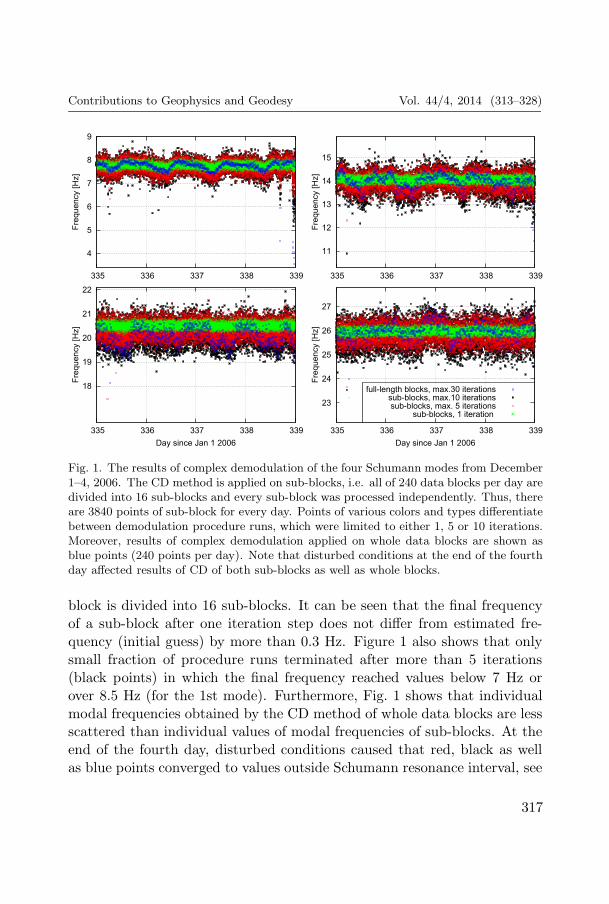
The first results of application of the iterative CD method on sub-blockscan be found in Ondraskova and Sevcık (2013) (Figs. 9–11 therein). Resultsof new calculations when the CD method has been applied on whole blocksare merged with former results and are presented here in Fig. 1. Green (lightgrey) points represent results of CD procedure runs applied to the sub-blockand limited to 1 iteration. Red points (dark grey) show the same procedureruns but maximal number of iterations was set 5. Black points are resultsof the same CD procedure runs but maximal number of iterations was 10.Blue points (dark points on light-gray background) in the middle representresults of CD procedure runs applied on whole data blocks. Shown are datafrom 4 complete days, i.e. 240 “blue” points per day (1 data block every 6minutes), and 240×16 = 3840 green, red and black points per day, as every

316


4

5

6

7

8

9

335 336 337 338 339

Freq

uenc

y [H

z]

11

12

13

14

15

335 336 337 338 339

Freq

uenc

y [H

z]

18

19

20

21

22

335 336 337 338 339

Freq

uenc

y [H

z]

Day since Jan 1 2006

23

24

25

26

27

335 336 337 338 339

Freq

uenc

y [H

z]


full-length blocks, max.30 iterationssub-blocks, max.10 iterationssub-blocks, max. 5 iterations

sub-blocks, 1 iteration

Fig. 1. The results of complex demodulation of the four Schumann modes from December1–4, 2006. The CD method is applied on sub-blocks, i.e. all of 240 data blocks per day aredivided into 16 sub-blocks and every sub-block was processed independently. Thus, thereare 3840 points of sub-block for every day. Points of various colors and types differentiatebetween demodulation procedure runs, which were limited to either 1, 5 or 10 iterations.Moreover, results of complex demodulation applied on whole data blocks are shown asblue points (240 points per day). Note that disturbed conditions at the end of the fourthday affected results of CD of both sub-blocks as well as whole blocks.

block is divided into 16 sub-blocks. It can be seen that the final frequencyof a sub-block after one iteration step does not differ from estimated fre-quency (initial guess) by more than 0.3 Hz. Figure 1 also shows that onlysmall fraction of procedure runs terminated after more than 5 iterations(black points) in which the final frequency reached values below 7 Hz orover 8.5 Hz (for the 1st mode). Furthermore, Fig. 1 shows that individualmodal frequencies obtained by the CD method of whole data blocks are lessscattered than individual values of modal frequencies of sub-blocks. At theend of the fourth day, disturbed conditions caused that red, black as wellas blue points converged to values outside Schumann resonance interval, see

317


Fig. 1 for the 1st and 2nd modes.Another comparison of the two variants of the CD method can be found

in Fig. 2. Black points represent arithmetic mean of 16 frequencies obtainedby the CD method applied on all 16 sub-blocks where maximal number ofiterations was set to 10. Blue points again represent results of the CDmethod applied on whole data blocks where maximal number of iterationswas set to 30. The same whole (complete) data blocks were processed by theLorentzian fitting method, i.e. the modal frequencies were determined bycomputing DFT spectrum which was then fitted by the least-square methodby the sum of 5 Lorentz functions (Rosenberg, 2004) – violet points. Nat-urally, modal frequencies obtained as means of 16 sub-blocks vary from a

7.0

7.5

8.0

335 336 337 338 339

Freq

uenc

y [H

z]


mean of 16 subblocks,max.10 iter.full-length blocks,max.30 iter.

Lorenzians fitting

13.0

13.5

14.0

14.5

15.0

335 336 337 338 339

Freq

uenc

y [H

z]


mean of 16 subblocks,max.10 iter.full-length blocks,max.30 iter.

Lorenzians fitting

Fig. 2. Modal frequencies for days Dec. 1 to Dec. 4, 2006, obtained by 3 different methods.Black points – the iterative CD method applied on sub-blocks and subsequently averaged(240 point per day); blue points – results obtained by iterative CD method applied onwhole blocks, 240 per day; violet points – results of Lorentzian function fitting methodapplied on the same whole data blocks, 240 per day. Upper plot is for the 1st SR mode,lower plot for the 2nd SR mode. Note that all methods give unreasonable frequenciesbelow 7.2 Hz at the end of 4th day.

318


mean value of 7.8 Hz with smallest amplitude. The plots show that, as arule, “Lorentzian” values are most scattered of all methods. A great dis-turbance of unknown origin at the end of the 4th day caused significantdeviations of modal frequency values from usual values, which can be seenin Lorentzian values as well as in values of both variants of the CD methodused in this study.

4. Daily variation of SR

One of the goals of SR analysis is determination of the daily variation and thedaily frequency range (DFR) for a given month of a year. The DFR is thedifference between maximal and minimal value on the monthly mean dailyfrequency curve. The importance of DFR lies in the fact that this quantityhas direct relation to the geometrical (angular) global thunderstorm fociarea (Nickolaenko and Hayakawa, 2002; Ondraskova et al., 2011).

As an example, monthly mean daily variation obtained using the iterativeCD method applied on sub-blocks from our observatory data for January2007 were showed in Ondraskova and Sevcık (2013). It was showed thatdaily variation obtained by CD method when maximum number of itera-tions was 5 is practically the same as in the case when maximum numberof iterations was 10. That is why the latter variant alone with maximalnumber of iterations of 10 is used in the daily variation determinations pre-sented here.

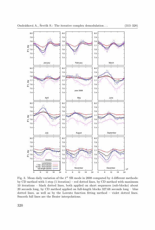
Monthly mean values of the 1st SR mode frequencies with a step of 30minutes for year 2008 are presented in Fig. 3. Then the Bezier interpolationcurve shows a smoothed monthly mean daily variation.

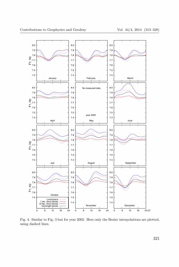
Results of four different methods of computation are depicted for com-parison. As expected, amplitude of the daily variation determined fromresults after 1 iteration step of CD (strictly speaking this is not the itera-tive CD method) is very small in all depicted months. This is true also foryear 2002 in Fig. 4, as well as for the 2nd SR mode (not depicted).

The greatest DFR gives the LFF method. The CD applied on the wholedata blocks (of the same length as LFF) gives daily variation of very closepattern and only slightly smaller DFR. It is interesting that in winter monthsthe curves of daily variation obtained by these two latter methods are also

319


Fig. 3. Mean daily variation of the 1st SR mode in 2008 computed by 4 different methods:by CD method with 1 step (1 iteration) – red dotted lines, by CD method with maximum10 iterations – black dotted lines, both applied on short sequences (sub-blocks) about20 seconds long, by CD method applied on full-length blocks 327.68 seconds long – bluedotted lines, as well as by the Lorentz function fitting method – violet dotted lines.Smooth full lines are the Bezier interpolations.

320


Fig. 4. Similar to Fig. 3 but for year 2002. Here only the Bezier interpolations are plotted,using dashed lines.

321


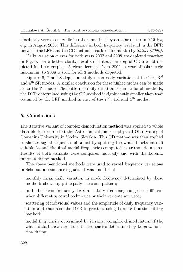
absolutely very close, while in other months they are afar off up to 0.15 Hz,e.g. in August 2008. This difference in both frequency level and in the DFRbetween the LFF and the CD methods has been found also by Satori (2009).

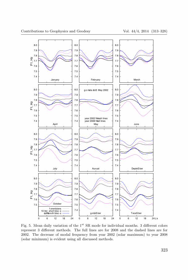
Daily variation curves for both years 2002 and 2008 are depicted togetherin Fig. 5. For a better clarity, results of 1 iteration step of CD are not de-picted in these graphs. A clear decrease from 2002, a year of solar cyclemaximum, to 2008 is seen for all 3 methods depicted.

Figures 6, 7 and 8 depict monthly mean daily variation of the 2nd, 3rd

and 4th SR modes. A similar conclusion for these higher modes can be madeas for the 1st mode. The pattern of daily variation is similar for all methods,the DFR determined using the CD method is significantly smaller than thatobtained by the LFF method in case of the 2nd, 3rd and 4th modes.

5. Conclusions

The iterative variant of complex demodulation method was applied to wholedata blocks recorded at the Astronomical and Geophysical Observatory ofComenius University in Modra, Slovakia. This CD method was then appliedto shorter signal sequences obtained by splitting the whole blocks into 16sub-blocks and the final modal frequencies computed as arithmetic means.Results of both variants were compared mutually and with the Lorentzfunction fitting method.

The above mentioned methods were used to reveal frequency variationsin Schumann resonance signals. It was found that

– monthly mean daily variation in mode frequency determined by thesemethods shows up principally the same pattern;

– both the mean frequency level and daily frequency range are differentwhen different spectral techniques or their variants are used;

– scattering of individual values and the amplitude of daily frequency vari-ation and thus also the DFR is greatest using Lorentz function fittingmethod;

– modal frequencies determined by iterative complex demodulation of thewhole data blocks are closer to frequencies determined by Lorentz func-tion fitting;

322


Fig. 5. Mean daily variation of the 1st SR mode for individual months. 3 different colorsrepresent 3 different methods. The full lines are for 2008 and the dashed lines are for2002. The decrease of modal frequency from year 2002 (solar maximum) to year 2008(solar minimum) is evident using all discussed methods.

323


Fig. 6. The same as Fig. 5 but for the 2nd SR mode.

324


Fig. 7. The same as Fig. 5 but for the 3rd SR mode.

325


Fig. 8. The same as Fig. 5 but for the 4th SR mode.

326


– no matter what spectral technique, calculated modal frequencies showclear decrease from 2002 (solar cycle maximum) to 2008 (solar cycle min-imum). Solar cycle variation in modal frequency is again greatest whenLorentz fitting is used Ondraskova et al., (2011).

Computational feasibility of the CD and LFF methods applied to data ofequal length is comparable. Modal frequency computation by CD methodusing short data sequences is fasted likely due to lower number of necessaryiteration steps.

Comparison of both methods as to the accuracy of modal SR frequencydetermination is obviously possible solely when an adequate artificial signalis processed, which is a mixture of different waves with varying amplitudesand phases, noise and with a dominant Schumann mode of known frequency.This comparison has not been done in this work and will be a subject offuture research.

Acknowledgments. Our sincere thanks go to the staff of AGO observatory

for invaluable help in experimental arrangement. We thank also to Ladislav Rosenberg,

who provided us with valuable advices and help in computer programming. The au-

thors acknowledge the remarks to the text of this paper from Pavel Kostecky. This

work was supported by the Slovak Research and Development Agency under the contract

No. APVV-0662-12. The authors also thank to the Slovak Scientific Grant Agency VEGA

for financial support under the grant No. 1/0859/12.

References

Childers D. G., Pao M. T., 1972: Complex Demodulation for Transient Wavelet Detectionand Extraction. IEEE Trans., AU–20, 295–308.

Draganova R., Popivanov D., 1999: Assessment of EEG Frequency Dynamics Using Com-plex Demodulation. Physiol. Res., 48, 157–165.

Gasquet H., Wootton J., 1997: Variable–frequency complex demodulation technique forextracting amplitude and phase information. Rev. Sci. Instrum., 68, 1111–1115.

Hao Y.-L., Ueda Y., Ishii N., 1992: Improved procedure of complex demodulation andapplication to frequency analysis of sleep spindles in EEG. Med. & Biol. Eng. &Comput., 30, 406–412.

Kostecky P., Ondraskova A., Rosenberg L., Turna L’., 2000: Experimental setup forthe monitor-ing of Schumann resonance electric and magnetic field variations atthe Geophysical Observatory at Modra-Piesok. Acta Astron. et Geophys. Univ.Comenianae, XXI–XXII, 71–92.

327


Lee J.-K., Park Y.-S., 1994: The Complex Envelope Signal and an Application to Struc-tural Modal Parameters Estimation. Mechanical Systems and Signal Processing, 8,2, 129–144.

Madden T., Thompson W., 1964: Low-Frequency Electromagnetic Oscillations in theEarth-Ionosphere Cavity. Res. Rept. Project NR-371-401, Geophysics Laboratory,Cambridge, Mass., 105 p.

Mushtak V. C., Williams E. R., 2008: An Improved Lorentzian Technique for EvaluatingResonance Characteristics of Earth-Ionosphere Cavity. Atmospheric Research, doi:10.1016/j.atmosres.2008.08.013

Myers A. P., Orr D., 1995: ULF Wave Analysis and Complex Demodulation. Proc. of theCluster Workshop on Data Analysis Tools, Braunschweig, Germany 28 - 30 Sept.1994 (ESA SP-371, June 1995), 23–32.

Nickolaenko A. P., Hayakawa M., 2002: Resonances in the Earth–Ionosphere Cavity,Kluwer Academic Publishers, Dordrecht, 362 p.

Ondraskova A., Kostecky P., Sevcık S., Rosenberg L., 2007: Long-term observationsof Schumann resonances at Modra Observatory. Radio Sci., 42, RS2S09, doi:

10.1029/2006RS003478

Ondraskova A., Sevcık S., Kostecky P., 2011: Decrease of Schumann resonance frequenciesand changes in the effective lightning areas toward the solar cycle minimum of 2008–2009. Journal of Atmospheric and Solar-Terrestrial Physics, 73, 534–543.

Ondraskova A., Sevcık S., 2013: The Determination of Schumann Resonance Mode Fre-quencies using Iterative Procedure of Complex Demodulation. Contrib. Geophys.Geod., 43, 4, 305–326.

Rosenberg L., 2004: Data processing methodology of the electric and magnetic compo-nents of the Schumann resonances at Modra observatory. Acta Astron. et Geophys.Univ. Comenianae, XXV, 1–8.

Satori G., Szendroi J., Vero J., 1996: Monitoring Schumann resonances I. Methodology.J. Atmos. Terr. Phys., 58, 1475–1481.

Satori G., 1996: Monitoring Schumann resonances II. Daily and seasonal frequency vari-ations. J. Atmos. Terr. Phys., 58, 1483–1488.

Satori G., 2009. Private communication.

Vero J., Szendroi J., Satori G., Zieger B., 2000: On Spectral Methods in SchumannResonance Data Processing. Acta Geod. Geophys. Hung., 35, 2, 105–132.

Williams E. R., Mushtak V. C., Nickolaenko A. P., 2006: Distinguishing IonosphericModels Using Schumann Resonance Spectra, J. Geophys. Res., 111, D 16107, doi:10.1029/2005JD006944.

328

Date post:	01-Mar-2022
Category:	Documents
Upload:	others
View:	2 times
Download:	0 times

The iterative complex demodulation applied on short and ...

Documents