The Lid-Driven Cavity’s Many Bifurcations – A Study of How and Where They Occur by Michael W. Lee Department of Mechanical Engineering and Materials Science Duke University Date: Approved: Earl H. Dowell, Supervisor Lawrie N. Virgin Thomas P. Witelski Thesis submitted in partial fulfillment of the requirements for the degree of Master of Science in the Department of Mechanical Engineering and Materials Science in the Graduate School of Duke University 2017
Transcript
The Lid-Driven Cavity’s Many Bifurcations – AStudy of How and Where They Occur
by
Michael W. Lee
Department of Mechanical Engineering and Materials ScienceDuke University
Date:Approved:
Earl H. Dowell, Supervisor
Lawrie N. Virgin
Thomas P. Witelski
Thesis submitted in partial fulfillment of the requirements for the degree ofMaster of Science in the Department of Mechanical Engineering and Materials
Sciencein the Graduate School of Duke University
2017
Abstract
The Lid-Driven Cavity’s Many Bifurcations – A Study of
How and Where They Occur
by
Michael W. Lee
Department of Mechanical Engineering and Materials ScienceDuke University
Date:Approved:
Earl H. Dowell, Supervisor
Lawrie N. Virgin
Thomas P. Witelski
An abstract of a thesis submitted in partial fulfillment of the requirements for thedegree of Master of Science in the Department of Mechanical Engineering and
Materials Sciencein the Graduate School of Duke University
Dr. E. Dowell is thanked for his invaluable mentorship and expertise. Dr. M.
Balajewicz is thanked for his regular guidance. Appreciation is extended to Drs. H.
Greenside, L. Virgin, and T. Witelski for their consultation. Lab members K. M. K.
Bastos, D. Levin, and K. McHugh are acknowledged for their willingness to engage
in discussion throughout this project’s span. This research is funded through the
National Science Foundation.
xi
1
Introduction
Thought is only a flash between two long nights, but this flash is every-
thing. – Henri Poincare
What causes the flash – the change – in a dynamical system? How and why
nonlinear dynamical systems progress between qualitatively different states has long
been a topic of research for scientists and engineers. Such bifurcations govern the dy-
namics of systems ranging from bridges in crosswinds to the stock market to chirping
cicadas in fields (Strogatz, 2014). In general, bifurcations can exist in systems which
are governed by nonlinear equations. Some systems are more approximately linear
than others, with scientists and engineerings achieving varying degrees of success
in applying these linear representations to real problems. A particular dynamical
system whose nonlinearity has long confounded scientists and engineers is that of a
fluid flow.
The nonlinear dynamics of fluid flows has been a subject of research for sev-
eral centuries. Leonardo da Vinci recorded these dynamics in illustrations dated
near the beginning of the 16th century (Figure 1.1). The efforts of Poincare, Euler,
1
d’Alambert, Cauchy, Navier, Stokes, Prandtl, the Wrights, Richardson, Hopf, Kol-
mogorov, Lorenz, and many others have resulted in a range of theories and a wealth
of data upon which contemporary fluids research is based.
Figure 1.1: da Vinci’s illustration of turbulence (Monaghan & Kajtar, 2014).
The highly nonlinear nature of fluid flows is the crux of the system’s complexity.
The governing equations of fluid flows (in the form of mass, momentum, and energy
conservation) are, as far as is currently understood, unsolvable from an analytical
perspective. As such, approximate methods and theories are often the best that
research can produce. Increasingly powerful computers allow more intricate simula-
tions to be performed, but as a flow becomes turbulent its dynamics become higher
in dimension. The exact simulation of even simple fluids engineering problems would
require computational resources predicted to not be available for more than a century
– and that is only if current computing performance trends continue.
There are, however, ways of analyzing such confounding systems without relying
on brute-force approximations of unsolvable equations. This is one of the goals of
nonlinear dynamical studies like that in this report. Observing the system, either
through computer simulation or physical experiment, allows for bifurcations, attrac-
tor basins, and so on to be identified without ever solving the system of equations in
closed-form. In identifying the qualitative behavior of a system, e.g. if and where bi-
2
furcations occur, nonlinear dynamicists can draw conclusions and predictions about
the system’s nature. For example, in the 1960’s a graduate student at MIT was
studying a simplified model of weather patterns in the form of large, atmospheric ed-
dies; from these model studies, the field of chaos theory was born. The fruits of chaos
theory have since affected everything from computer graphics to fluid modeling.
A recent stride towards understanding the dynamics of fluid flows transitioning
to turbulence was made when Ruelle & Takens (1971) explained how a near-infinite
number of bifurcations were not required to move a flow from an asymptotically
steady state to a fully chaotic one, as had previously been believed (Landau, 1944;
Hopf, 1948). Their scenario, which involves a flow’s progression from steady, time-
independent laminar flow to periodic limit cycle oscillations to chaotic oscillations,
has been accepted in part due to its ability to describe the dynamics of the Taylor-
Couette flow as explored by Gollub & Swinney (1975). The present work will simi-
larly study the sequence of bifurcations that brings a canonical flow, the regularized
2D lid-driven cavity, from stable linear dynamics to chaotic dynamics. Historically,
the first Hopf bifurcation, characterized by the appearance of a limit cycle, has re-
ceived a great deal of attention (Peng et al., 2003; Shen, 1991; Shankar & Deshpande,
2000). This paper will characterize a flow’s progression from limit cycle periodicity
to chaos just as previous work has characterized the progression from stable steady
flow to periodic limit cycles.
1.1 The Regularized 2D Lid-Driven Cavity
The regularized 2D lid-driven cavity, described mathematically in §2, is a well known
internal flow problem. Shankar and Deshpande, in their review of the cavity’s dy-
namics (Shankar & Deshpande, 2000), state that this particular flow problem can
exhibit virtually all naturally occurring incompressible flow phenomena, including
chaotic flow. There are several permutations of the lid-driven cavity problem; this
3
study will focus on the 2D regularized species.
The lid-driven cavity is an internal flow problem in which a box of arbitrary aspect
ratio is driven by a velocity profile specified on one of its boundaries. By convention,
this moving boundary is normally on the top of the cavity. There are 2D as well as
3D forms of the lid-driven cavity problem; the 2D version studied here is often used
as a numerical modeling test case to ensure a new program or modeling scheme has
been developed and implemented correctly. There is a wealth of literature on the
lid-driven cavity, perhaps most notably with 3D high-Reynolds number data from
both experimental (Prasad & Koseff, 1989) and numerical investigations (Deshpande
& Shankar, 1994b,a; Verstappen et al., 1994).
In an annual review on cavity flows (Shankar & Deshpande, 2000), the authors
emphasize one of the reasons why the 2D flow has been used as a test case for so
long: it is a relatively simple geometric problem that appears to exhibit virtually
all possible viscous 2D flow phenomena, including but limited to Hopf bifurcations,
corner vortices, periodic shedding, and chaotic flow. However, the difficulty in making
the 2D flows dynamically equivalent to even high-aspect ratio 3D flows (discussed
further in §2.2) is a crucial detail to note about cavity flows in general. The lack of
a physical equivalent, though, does not detract from the relevance of the 2D cavity
flow; its use as a test case and research tool has contributed to the study of fluid
physics for several decades (Shankar & Deshpande, 2000).
The 2D lid-driven cavity flow is often considered to be incompressible, which leads
to the flow’s Reynolds number being the dominant governing parameter. Unless
specified as a compressible cavity flow, a cavity flow presented in the literature can
be interpreted as an incompressible one. How the Reynolds number is defined and
varied in numerical simulations will be discussed in detail in the following sections.
Besides the Reynolds number, the flow’s dynamics can be manipulated in interest-
ing ways by changing the cavity’s aspect ratio. While many studies have investigated
4
the dynamics associated with different aspect ratios (Stremler & Chen, 2007; Gollub
& Benson, 1980), this research will limit its varying parameter to exclusively the
Reynolds number by considering only a square cavity. The square cavity also allows
many symmetries to develop within the flow; for example, the bottom corner vortices
are, when they are apparent, often mirror images of one another.
The cavity is regularized in that the flow profile defined on the cavity’s top bound-
ary goes to 0 at the lid boundaries to remove singularities in those corners. This
lid flow profile is the same as that used in Shen’s study of the cavity’s progression
through multiple Hopf bifurcations (Shen, 1991). In his work, Shen uses a similar
(spectral) computational framework to analyze the 2D lid-driven cavity and draws
now-established conclusions concerning the cavity’s behavior near the first critical
Reynolds number. Shen’s work identified Hopf bifurcations in the regularized cavity
as functions of Reynolds number, but did not study the flow at Reynolds numbers
above 15,500; the present work increases the Reynolds number further than Shen
chose to study with the understanding that stable limit cycles will become increas-
ingly difficult to obtain as the Reynolds number continues to increase. The resulting
observations agree with Shen within the range of his observed Reynolds numbers,
although the transition to chaos is observed at a higher Reynolds number than he
had predicted.
1.2 Report Outline
This report will progress from lower to higher Reynolds numbers in subsequent sec-
tions. The flow’s nonlinear characteristics before the first Hopf bifurcation will be
briefly considered. However, as there is a wealth of existing literature on this first
Hopf bifurcation, e.g. Peng et al. (2003), it will not be this paper’s primary focus.
The first Hopf bifurcation was observed near Re 10, 250, which aligns with the
findings of Shen (1991), who studied this same species of cavity flow. This first crit-
5
ical Reynolds number is understood to be higher than that of the cavity flow driven
by a constant lid velocity.
The periodic and quasi-periodic flow regimes will then be observed as the flow
progresses towards chaos. §5 will discuss why a more formal characterization of
chaos could not be performed; §6 and §7 will then identify the cavity flow’s route to
chaos with, respectively, Poincare sections and power spectrum analyses. A toroidal
bifurcation will be observed over a range of several thousand Reynolds numbers
(between Re 18, 000 and Re 23, 000) with a strong case of frequency entrainment
occurring near Re 21, 000.
A novel concept called frequency shredding will be introduced in an attempt
to explain how the flow progresses from stable limit cycles, through myriad quasi-
periodic states, and eventually to chaos. The concepts of frequency shredding and
entrainment together will explain all observed patterns in the flow’s progression to
chaos.
6
2
Problem Formulation
The regularized 2D incompressible square lid-driven cavity is most specifically what is
studied in this research. The cavity is regularized in that the boundary conditions do
not experience jump discontinuities in the top two corners, where the homogeneous
and inhomogeneous boundary conditions meet. More specifically, the inhomogeneous
boundary condition implemented in this research sets the horizontal velocity u and
its slope dudx
equal to 0. The implemented inhomogeneous boundary condition is of
the form
utop px 1q2px 1q2 (2.1)
which corresponds to the same inhomogeneous boundary condition implemented by
Shen in his study of the regularized cavity (Shen, 1991). The 2D cavity studied in this
research is illustrated in Figure 2.1. The remainder of this chapter will present the
theory and numerical methods implemented to simulate this system, with discussion
on the implications of the problem’s particular formulation, including its regularized
and 2D characteristics.
7
Figure 2.1: Regularized 2D lid-driven cavity formulation with vorticity contoursat characteristically low (left) and high (right) Reynolds numbers. Stream functionsampling locations are marked with X’s.
2.1 Governing Equations and their Nondimensionalization
The dimensional governing equations are
∇ ~u 0 (2.2a)
B~uBt p∇ ~uq ~u ∇P
ρ ν∇2~u (2.2b)
and the inhomogeneous boundary condition for the regularized lid-driven cavity is
u
x, y Ly
2, t
umaxfpx, y, tq . (2.3)
These can be nondimensionalized such that the constant, global Reynolds number ap-
pears exclusively in either the field equations or the boundary conditions. These two
8
dimensionless formulations represent the bases for two different studies in Reynolds
number perturbations; understanding how these two formulations differ is crucial to
understanding which physical experiment is most equivalent to the flows simulated
in this research.
In this derivation, the 2D lid-driven cavity will be defined with width Lx and
height Ly and with the origin centered within the cavity at Lx
2and Ly
2.
The formulation will begin from these vectorized, dimensional equations and
branch into two final forms: one with the Reynolds number in the field equations and
one with the Reynolds number in the boundary condition. The Reynolds number,
stream function ~Ψ Ψk, and the vorticity ~ω ωk are defined for this 2D flow as
follows.
Re umaxLyν
(2.4a)
~u ∇ ~Ψ (2.4b)
~ω ∇ ~u (2.4c)
Taking the curl of the velocity yields, with the above definitions in mind,
∇∇ ~Ψ
~ω .
This simplifies to Poisson’s Equation, which is an alternative form of Equation 2.2a.
∇2~Ψ ~ω (2.5)
Taking the curl of Equation 2.2b, keeping in mind the pressure term vanishes from
the vector identity ∇∇φ 0@φ where φ is a scalar function, one obtains
B~ωBt ∇ p∇ ~uq ~u ν∇2~ω . (2.6)
9
Recalling that the x- and y-components of the velocity vector ~u can be represented
as
ux BΨ
By , uy BΨ
Bx ,
then by applying Equation 2.5 one obtains
∇ p∇ ~uq ~u B~ΨBy
B~ωBx
B~ΨBx
B~ωBy . (2.7)
Applying Equation 2.7 to Equation 2.6 yields
B~ωBt
B~ΨBy
B~ωBx
B~ΨBx
B~ωBy ν∇2~ω . (2.8)
Equations 2.3, 2.5, and 2.8 thus form the final fully dimensional governing equations
and nonzero boundary conditions for the 2D incompressible regularized lid-driven
cavity in terms of the stream function and vorticity. For the remainder of this
derivation, the stream function and vorticity vectors will be represented as the mag-
nitudes of their k components for the sake of simplifying notation. Dimensionless
terms will be marked with a tilde.
The x- and y-coordinates will be nondimensionalized by the cavity’s dimensions.
rx x
Lx, ry y
Ly(2.9)
Equations 2.3, 2.5, and 2.8 thus become
u
x, y Ly
2, t
1
Ly
BΨ
Brypx,y
Ly2,tq
umaxfpx, y, tq , (2.10a)
1
L2x
B2Ψ
Brx2 1
L2y
B2Ψ
Bry2 ω , (2.10b)
BωBt
1
LxLy
BΨ
Bry BωBrx BΨ
Brx BωBry ν
1
L2x
B2ω
Brx2 1
L2y
B2ω
Bry2
. (2.10c)
10
From these three equations, the nondimensionalization branches based on the desired
location of the Reynolds number – either in the equations of motion or the boundary
conditions.
2.1.1 Branch 1: Reynolds Number in the Boundary Conditions
The stream function and velocity can be nondimensionalized as
rΨ Ψ
ν(2.11a)
ru u
umax. (2.11b)
Applying Equation 2.11a to Equations 2.10b and 2.10c yields, respectively,
ν
L2x
B2rΨBrx2
ν
L2y
B2rΨBry2
ω (2.12a)
BωBt
ν
LxLy
BrΨBry BωBrx BrΨ
Brx BωBry ν
1
L2x
B2ω
Brx2 1
L2y
B2ω
Bry2
. (2.12b)
This stream function nondimensionalization also transforms Equation 2.10a to its
final dimensionless form:
rux, y Ly2, t
BrΨ
Brypx,y
Ly2,tq
Re fpx, y, tq . (2.13)
The vorticity terms in Equations 2.12a and 2.12b can then be nondimensionalized
by
rω L2yω
ν. (2.14)
Applying this along with Equation 2.25 yields a dimensionless continuity equation:
r∇2rΨ rω . (2.15)
11
Applying these same manipulations to Equation 2.12b yields
νL2y
BrωBt
ν2LyLx
BrΨBry BrωBrx BrΨ
Brx BrωBry ν2 r∇2rω . (2.16)
Nondimensionalizing t by
rt νt
L2y
(2.17)
and dividing by the common ν2 term yields the final dimensionless form of the
Navier-Stokes equation for this branch:
BrωBrt Ly
Lx
BrΨBry BrωBrx BrΨ
Brx BrωBry r∇2rω . (2.18)
Equations 2.13, 2.15, and 2.18 (rewritten below for reference) thus form the dimen-
sionless foundation for a 2D incompressible regularized lid-driven cavity with the
global Reynolds number appearing in the boundary conditions.
rux, y Ly2, t
BrΨ
Brypx,y
Ly2,tq
Re fpx, y, tq
r∇2rΨ rωBrωBrt Ly
Lx
BrΨBry BrωBrx BrΨ
Brx BrωBry r∇2rω
(2.13)
(2.15)
(2.18)
2.1.2 Branch 2: Reynolds Number in the Field Equations
Starting again from Equations 2.10a, 2.10b, and 2.10c, an alternative nondimension-
alization of the stream function can be applied:
rΨ Ψ
Lyumax(2.20)
12
The velocity is still, however, nondimensionalized with Equation 2.11b. Applying
Equation 2.20 to Equations 2.10b and 2.10c yields, respectively,
LyumaxL2x
B2rΨBrx2
umaxLy
B2rΨBry2
ω , (2.21a)
BωBt
umaxLx
BrΨBry BωBrx BrΨ
Brx BωBry ν
1
L2x
B2ω
Brx2 1
L2y
B2ω
Bry2
. (2.21b)
Applying Equations 2.20 and 2.11b to Equation 2.10a yields its final dimensionless
form in this branch.
rux, y Ly2, t
BrΨ
Brypx,y
Ly2,tq
fpx, y, tq (2.22)
In order to complete the nondimensionalization of Equation 2.21a, the dimensionless
vorticity is defined as
rω ωLyumax
. (2.23)
Thus, Equation 2.21a becomes
L2y
L2x
B2rΨBrx2
B2rΨBry2
rω . (2.24)
Defining the operator r∇2 as
r∇2 L2y
L2x
B2
Brx2 B2
Bry2(2.25)
yields the final dimensionless continuity equation
r∇2rΨ rω . (2.26)
Turning now to the next equation, nondimensionalizing the vorticity in Equation
2.21b yields
umaxLyBrωBt
u2maxLyLx
BrΨBry BrωBrx BrΨ
Brx BrωBry νumax
Lyr∇2rω, (2.27)
13
which requires one further step of nondimensionalization. Defining
rt umaxt
Ly(2.28)
and dividing all terms by u2max forms the final dimensionless form of the Navier-Stokes
equation in this branch:
BrωBrt Ly
Lx
BrΨBry BrωBrx BrΨ
Brx BrωBry
r∇2rωRe
. (2.29)
Equations 2.22, 2.26, and 2.29 (rewritten below for reference) thus form the dimen-
sionless foundation for a 2D incompressible regularized lid-driven cavity with the
global Reynolds number now appearing in the field equations.
rux, y Ly2, t
BrΨ
Brypx,y
Ly2,tq
fpx, y, tq
r∇2rΨ rωBrωBrt Ly
Lx
BrΨBry BrωBrx BrΨ
Brx BrωBry
r∇2rωRe
(2.22)
(2.26)
(2.29)
2.2 Physical Interpretation
The physical consequences of these two dimensionless formulations are worth consid-
ering. In the first, the Reynolds number appears only in the inhomogeneous boundary
condition. Thus, a change in the global Reynolds number can be likened to a physical
experiment in which the lid velocity is perturbed. However, in such a physical exper-
iment it may be difficult to keep the flow appropriately two-dimensional. To be 2D
in a physical setting, the flow must have its strain and vorticity vectors orthogonal
everywhere. Otherwise, vortex stretching and other 3D phenomena will affect the
flow’s dynamics especially at higher Reynolds numbers. Driving a cavity boundary
14
with, for example, a moving belt would require extremely low tolerances to prevent
the moving parts from themselves causing 3D effects. (The static components would
be relatively less problematic as long as the imperfections are isotropic.) To demon-
strate this, one can consider the vorticity equation (derived in Appendix A) that can
be derived directly by taking the curl of the homogeneous Navier-Stokes equations:
B~ωBt p~u ∇q ~ω p~ω ∇q ~u ν∇2~ω . (2.31)
The first term on the right side, p~ω ∇q ~u, is equivalent to the inner product of the
vorticity vector and the strain tensor; this is the vortex stretching term which is
argued by some to be a fundamental aspect of turbulence (Pope, 2000; Tennekes &
Lumley, 1972). In 2D flows, these two terms are orthogonal everywhere and therefore
this inner product vanishes. In other words, there is identically no vortex stretching
in 2D flows. However, if the velocity profile in Cartesian coordinates is prescribed as
~upx, yq pfpxq δq i ηj ξk (2.32)
where fpxq is a known function and δ, η, and ξ are small fluctuations (e.g. from
physical imperfections) in the x, y, and z directions, then the vortex stretching term
becomes
p~ω ∇q ~u BξBy
BηBzdf
dxi (2.33)
if products of small terms, including products of disturbance derivatives, are ap-
proximated to zero (i.e. the system is linearized about the driving function). As
such, where the velocity profile’s x-derivative is not zero, small imperfections in the
y and z directions will compound and cause non-negligible vortex stretching, thus
making the flow 3D in long, finite time. The regularized lid-driven cavity has such
a prescribed non-constant velocity profile on one of its sides, and as such an experi-
15
mentalist would find it difficult to maintain appropriately 2D flow for this problem.1
Adding to this the complexity of physically driving a boundary with spatially non-
uniform distribution to simulate a regularized cavity and at a temporally fluctuating
rate to simulate perturbations in the Reynolds number, it would be challenging to
realize a regularized lid-driven cavity that is driven by a physically moving boundary.
In the second dimensionless formulation, the Reynolds number appears instead
in the field equations. Therefore, a change in the global Reynolds number instead
likens to a cavity whose entire volume instantaneously changes its kinematic vis-
cosity, length scale, or velocity. Changing the length scale would be very difficult
to accomplish without 1) inciting the same 3D phenomena discussed above and 2)
turning (with tongue in cheek) the lid-driven cavity into a lids-driven cavity by hav-
ing multiple boundaries move as they grow. The length scales and velocity field are
also apparent in the field equations outside of the Reynolds number, so changing
these would affect the flow’s dynamics in coupled ways beyond just the changed
Reynolds number. Thus, a change in the field equations’ Reynolds number is most
effectively likened to a change in the cavity’s global kinematic viscosity. Maintain-
ing the flow’s incompressibility in turn makes the second formulation most like a
physical experiment in which the cavity’s global dynamic viscosity can be changed.
Such an experiment was explored several decades ago (Andrade & Dodd, 1946), but
even in this rare experimental setup the viscosity was changed non-globally based
on the distribution of electrodes. Minimal change to viscosity was also observed in
the plane of the fluid’s two-dimensional motion – thus causing the flow to become
3D where the viscosity changed. Therefore, one would need to construct a physical
experiment in which one boundary is driven at a spatially non-uniform but tempo-
rally constant rate and the cavity volume is between high-voltage electrodes spaced
1 An interesting observation is that this linearization does not rule out the possibility of anexperimental 2D lid-driven cavity with constant lid velocity. This, however, is not the type ofcavity studied here.
16
carefully enough to elicit uniform in-plane changes to viscosity and these changes in
viscosity do not themselves elicit 3D flow behavior. Considering the low feasibility
of such a physical experiment, the second nondimensionalization does not appear to
be more easily physically realizable than the first.
Perturbing the global Reynolds number raises another concern as well: that bifur-
cations as functions of Reynolds number may be incorrectly identified.2 A flow will
be considered that is arbitrarily close to bifurcating, i.e. Re Recrit ε where Recrit
is the critical Reynolds number at which the bifurcation occurs. If the Reynolds
number is perturbed such that ∆Re ¡ ε, then the flow will bifurcate. However, if
the Reynolds number is perturbed such that ∆Re ε, then the flow will not bifur-
cate. Thus, given an unknown proximity to the critical Reynolds number, a finite
number of perturbations would undoubtedly lead to an inaccuracy (however small)
in the identification of the Reynolds numbers associated with bifurcations.
A third type of cavity driving not considered in the above governing equations or
their resulting nondimensionalizations is the inclusion of a body force. The homoge-
neous Navier-Stokes equations were used as the basis of these nondimensionalizations,
but an inclusion of a body forcing term would allow the field to be driven in another
way. This body force would have to be defined in such a way that it could not be rep-
resented as some potential, otherwise it would vanish as the pressure term did in the
nondimensionalization. There is a wealth of literature on implementing these kinds
of body forces experimentally using magnetic fields to induce velocities via Lorentz
forces (Clercx & van Heijst, 2009; Kelley & Ouellette, 2011). However, perturbations
in these ultimately nondimensionalized body forces would again couple changes in
the velocity field – a local parameter identifying the flow’s dynamics – to the global
Reynolds number. Thus, studying the flow’s nonlinear dynamics as a function of the
global Reynolds number, which is the underlying goal of this research, would again
2 Appreciation is extended to Dr. M. Balajewicz for his explanation of this insight.
17
become difficult.
It appears, then, that any experimental method of perturbing the regularized
lid-driven cavity, or even physically studying it at all, is very challenging. This sen-
timent is expressed in so many words in an annual review of cavity flows (Shankar
& Deshpande, 2000); more specifically, studies by Koseff and Street explored the
ways in which 2D and high-aspect ratio 3D cavity flows differed, with the conclu-
sion that they are rarely, if ever, equivalent (Koseff & Street, 1984a,b). Chien et al.
(1986) also studied experimental 2D cavity flows, up to and including some chaos
characterization, but no observed flows were regularized; the inhomogeneous bound-
ary conditions were always spatially constant, albeit potentially fluctuating in time.
However, this does not necessarily detract from the validity of a numerical study in
which the global Reynolds number is changed in a way that is physically intractable.
Regarding the study of the regularized lid-driven cavity, Shen (1991) stated that
[a]lthough this regularization is less physical, it is expected that the regu-
larized driven cavity flow preserves qualitatively the dynamical properties
of the driven cavity flow. However . . . we would expect that if the reg-
ularized driven cavity flow exhibits Hopf bifurcations at certain critical
Reynolds number, then the driven cavity flow will also exhibit Hopf bi-
furcations at a smaller critical Reynolds number.
Shen explains well how the qualitative dynamics of the flow are not necessarily
altered simply because of a less physically feasible domain or method of excitation.
With this understanding in mind, the computationally simple method of changing
the global Reynolds number within the field equations (i.e. a problem based on
the boxed equations at the end of §2.1.2) was implemented for this study with the
understanding that the exact critical Reynolds numbers would not be identified. The
inability to identify exact critical Reynolds numbers was considered of negligible
18
consequence, as this research is more concerned with the flow’s dynamics between
critical Reynolds numbers than precisely at the critical Reynolds numbers.
2.3 Computational Model
Equations 2.22 (the inhomogeneous boundary condition), 2.26 (Poisson’s equation),
and 2.29 (an advective-diffusion equation) are used as the basis for a numerical sim-
ulation of the incompressible 2D regularized square lid-driven cavity. With a square
aspect ratio, the length ratio in the advective-diffusion equation goes to 1. The abso-
lute cavity dimensions were set to Lx Ly 2 such that the upper (inhomogeneous)
boundary condition occur at y 1.
The volume is discretized using an nth-order Chebyshev pseudo-spectral collo-
cation scheme – the same as was used by Shen (Shen, 1991) in his study of the
regularized lid-driven cavity. The flow is then marched in time, initially from rest,
using the second-order backward-difference (2BDF) temporal scheme. A detailed
computational framework is presented in Appendix B3 and is the same as was im-
plemented in a previous study using this flow regime to test a model-order reduction
strategy (Balajewicz et al., 2013).
2.4 Simulated Flows
The flow’s initial conditions are that of a still cavity, i.e. the stream function and
vorticity at all points are set to 0. The flow is then allowed to reach a statistically
steady state, as determined by a stabilized maximum and minimum within the recent
time history at the cavity’s center. Mathematically, the system is considered to be
in a steady state if
max rΨcppτf T q : τf qs max rΨcppτf 2T q : pτf T qqs ε and
min rΨcppτf T q : τf qs min rΨcppτf 2T q : pτf T qqs ε(2.34)
3 This appendix was prepared by M. Balajewicz.
19
where Ψc is the stream function at the cavity center, T is a sample time interval,
taken here to be 200 dimensionless time units τ , τf is the final time step computed
thus far, and ε is a predetermined allowable error margin. In this study, ε 1012 for
flow responses up to the first Hopf bifurcation, i.e. where a limit cycle first appeared.
At this point in the simulation, the flow can be considered steady-state at the
specified Reynolds number. By this, it is meant that the mean flow is considered to be
stabilized, though steady oscillations or unsteady fluctuations about that mean are
certainly present at higher Reynolds numbers. To study the dynamics at the specified
Reynolds number, the flow is then perturbed in various ways. The responses to these
different perturbations allows for the performance of a local dynamics analysis within
the broad Reynolds number range of interest. This is because the responses from
rest have long-time transient responses that more significantly affect the qualitative
nature of the response.
Responses to a step change in Reynolds number were only simulated at flows
with asymptotic linear behavior, i.e. flows below the first critical Reynolds number.
These step responses are discussed in §4.3. The step perturbation was simulated by
increasing the Reynolds number by 1%
Restep pτ0,stepq 1.01Re0 pτf,restq (2.35)
at the final simulated time of the response from rest τf,rest. The system was then
allowed to reach a new steady state at this slightly higher Reynolds number, as
determined by the same ε 1012 condition.
Responses to impulses in Reynolds number were also simulated. A small impulse
change in Reynolds number with magnitude A
Reimp,A pτ0,impq Re0 A
Reimp,A pτ0,imp τq Re0
(2.36)
was simulated to last one dimensionless time unit τ , or equivalently 1∆t
time steps
20
of length ∆t. Non-unit impulses where A 1 were also studied only for sub-critical
Reynolds numbers and are discussed in §4.2. Unit impulses where A 1 were
simulated across the entire Reynolds number range of interest and are the basis for
all high-Reynolds number analyses.
As was discussed above, this change in the global Reynolds number, which lies
in the dimensionless field equations, affects the entire cavity instantaneously. Where
a limit cycle is present, all perturbation responses were computed for 5,000 dimen-
sionless time units τ for consistent resolution in the frequency spectrum.
2.5 Data Presented
Excepting the resolution study in §3, none of the responses simulated from rest will
be presented. Instead, responses to select perturbation types will form the data
set for each section. For example, the power spectrum analysis presented in §7 is
based solely on responses from unit impulses in Reynolds number. When plots are
presented with dimensionless time τ as an axis, readers should note that τ 0
indicates the beginning of the time history for the perturbation response, which is
more formally τf for the response computed from rest.
This research focuses on the temporal – not spatial – system behavior as a function
of Reynolds number. As such, rather than studying the behavior of the entire control
volume, certain cavity locations were probed to identify potentially representative
coordinates that would reduce the studied domain from a discretized continuum to a
single scalar value, i.e. the stream function at that location. The total kinetic energy
Eptq 1
2
¼|~u|2 dA 1
2
¸i, j
u2ij v2
ij
Aij
where uij and vij are, respectively, the horizontal and vertical velocity components at
the ith and jth volume locations was also tested as a potential observational lens. In
21
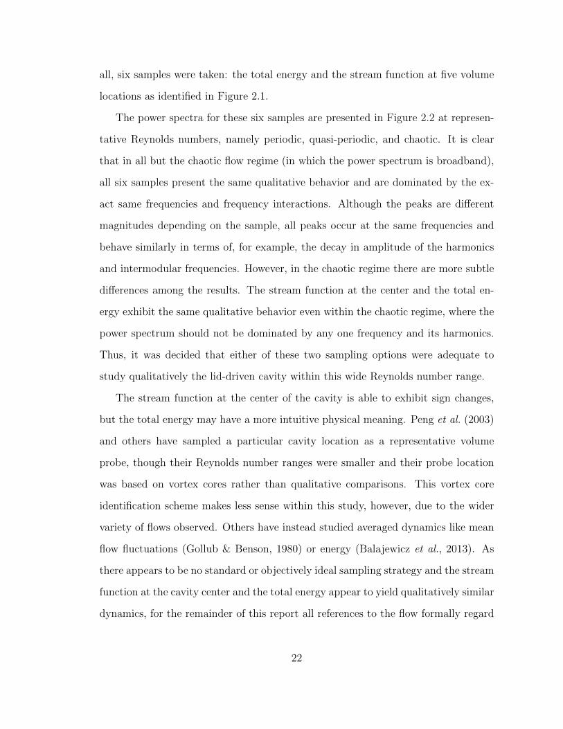
all, six samples were taken: the total energy and the stream function at five volume
locations as identified in Figure 2.1.
The power spectra for these six samples are presented in Figure 2.2 at represen-
tative Reynolds numbers, namely periodic, quasi-periodic, and chaotic. It is clear
that in all but the chaotic flow regime (in which the power spectrum is broadband),
all six samples present the same qualitative behavior and are dominated by the ex-
act same frequencies and frequency interactions. Although the peaks are different
magnitudes depending on the sample, all peaks occur at the same frequencies and
behave similarly in terms of, for example, the decay in amplitude of the harmonics
and intermodular frequencies. However, in the chaotic regime there are more subtle
differences among the results. The stream function at the center and the total en-
ergy exhibit the same qualitative behavior even within the chaotic regime, where the
power spectrum should not be dominated by any one frequency and its harmonics.
Thus, it was decided that either of these two sampling options were adequate to
study qualitatively the lid-driven cavity within this wide Reynolds number range.
The stream function at the center of the cavity is able to exhibit sign changes,
but the total energy may have a more intuitive physical meaning. Peng et al. (2003)
and others have sampled a particular cavity location as a representative volume
probe, though their Reynolds number ranges were smaller and their probe location
was based on vortex cores rather than qualitative comparisons. This vortex core
identification scheme makes less sense within this study, however, due to the wider
variety of flows observed. Others have instead studied averaged dynamics like mean
flow fluctuations (Gollub & Benson, 1980) or energy (Balajewicz et al., 2013). As
there appears to be no standard or objectively ideal sampling strategy and the stream
function at the cavity center and the total energy appear to yield qualitatively similar
dynamics, for the remainder of this report all references to the flow formally regard
22
(a) Periodic response at Re 12, 000. (b) Quasi-periodic response at Re 17, 000.
(c) Chaotic response at Re 25, 000.
Figure 2.2: Power spectra at different sampling locations.
the stream function (or velocity in the case of §6) at the cavity center:
Ψpx, y, tq Ñ Ψp0, 0, tq Ψcptq . (2.37)
23
3
Spatial and Temporal Resolution Study
As is the case in any computational study, discretization error had to be mitigated
as best as possible before any conclusions could be made. Ensuring the system
dynamics would not change with increased resolution was thus the first step taken
in this study. To observe the solution’s sensitivity to discretization error, the cavity
flow was simulated at the highest Reynolds number of interest, namely Re 25, 000,
with three different spatial resolutions. Although a formal resolution study, e.g. a
Richardson extrapolation, was not able to be performed, the dynamics captured by
the simulated cavity were found to be in agreement with that of existing literature.
3.1 Numerical Stability
The convergence study had only limited success due to inherent instabilities in the
Python 3 code developed to simulate the cavity system. For reasons yet unknown to
the author, coarse and fine1 spatial resolutions were asymmetrically unstable. The
coarser resolutions led to stream function matrices filled with 8; the finer resolu-
1 At Re 25, 000, coarse unstable grids had fewer than 100 nodes per cavity dimension; fineunstable grids had more than 130 nodes per cavity dimension.
24
tions led to stream function matrices filled with 8. Two factors are of particular
interest: 1) the nature of the numerical divergence and 2) the fact that both coarse
and fine grids showed such behavior.
The solutions were observed to behave very well for the first n2 time steps, with
all cases being started from rest and near-identical behavior being observed between
even significantly different resolutions. Then, from time step n to time step n 1,
the solution would move from Ψ O p101q to Ψ O p10100q and within a few
more time steps numerical 8 would populate the entire stream function matrix.
This divergence occurred at the same number of time steps regardless of how many
times the program was executed.
What’s more, the number of stable time steps n appeared to be a function of the
spatial resolution, implying that some “centrally stable” resolution existed. As the
resolution moved away from this special value, the solution was observed to diverge
– always within only a few time steps – after fewer and fewer n time steps. In
other words, the solution became more quickly divergent with either increasing or
decreasing spatial resolution.
The cause of this numerical instability was, naturally, investigated. The first
possible cause that was studied was compounding numerical error, in which the
natural O p1016q noise in computations eventually leads to inaccurate calculations
on the order of the system of interest. However, for systems of such small resolutions
and such few time steps, this compounding error should not be a significant source of
error. Also, compounding error would not usually manifest as a sudden divergence
within a single time step, nor would it appear just as dramatically for coarser grids,
where there are even fewer calculations being performed.
A memory overflow issue may cause such a dramatic divergence within a single
time step. However, it is likely that such an overflow would not be so consistent in
2 At Re 25, 000, the number of stable time steps was O104
.
25
its appearance. Several simulations of finer and coarser grids consistently yielded the
exact same number of stable time steps before diverging. Also, the fact that some
resolutions near the “centrally stable” one seemed to be completely stable rules out
memory overflow as the source of the instability.
This divergence as a function of spatial resolution was observed in not only the
Python 3 code that was developed for this research, but also in the MatLab code
upon which the Python 3 code was based. The MatLab code was implemented by
Balajewicz et al. (2013) at a higher Reynolds number than was simulated in this
study as a part of their reduced-order model testing, though in this paper no grid
convergence details were included. However, at the time step ∆t 0.001 and number
of nodes per cavity side Nx 27 implemented in this previous research, the MatLab
and Python codes were both observed to be stable, even in long (n O p107q) time.
3.2 Qualitative Resolution Analysis
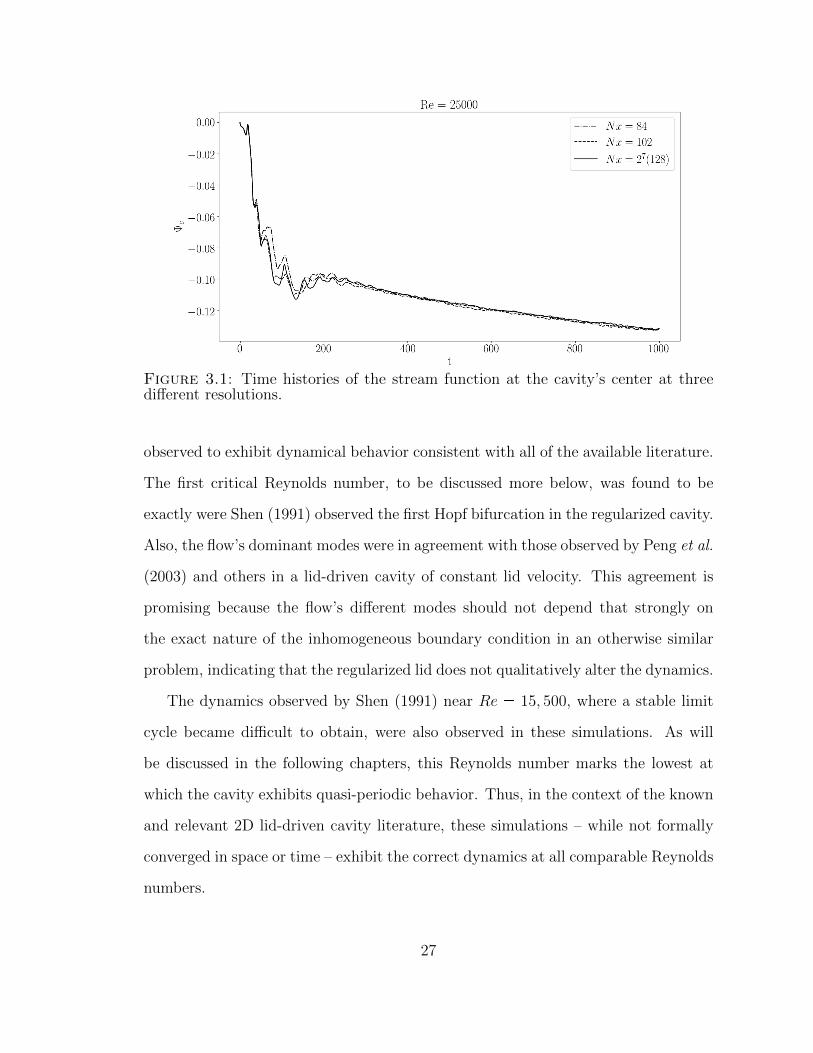
Cavities with three different spatial resolutions were ultimately simulated that were
as different in resolution as the software could stably resolve. The short-term tran-
sient time histories of all three are presented in Figure 3.1. As discretization error
is expected to be worst during the transient stages of the responses, each grid was
only assessed out to 1,000 dimensionless time units, or n 1 106 time steps.
The largest difference between the long time behavior simulated by the coarse
and fine grids was approximately 1.5 103. This same difference between the
medium and fine grids was approximately 1.9 103. Thus, there was minimal
change in results even with the most significant changes in resolution that were
possible. There were also minimal differences between the power spectra of these
three transient trajectories. Thus, the finest stable resolution of ∆t 0.001 and
Nx 27 was implemented for the remainder of this study.
The selected resolution, whose fidelity could not be adequately quantified, was
26
Figure 3.1: Time histories of the stream function at the cavity’s center at threedifferent resolutions.
observed to exhibit dynamical behavior consistent with all of the available literature.
The first critical Reynolds number, to be discussed more below, was found to be
exactly were Shen (1991) observed the first Hopf bifurcation in the regularized cavity.
Also, the flow’s dominant modes were in agreement with those observed by Peng et al.
(2003) and others in a lid-driven cavity of constant lid velocity. This agreement is
promising because the flow’s different modes should not depend that strongly on
the exact nature of the inhomogeneous boundary condition in an otherwise similar
problem, indicating that the regularized lid does not qualitatively alter the dynamics.
The dynamics observed by Shen (1991) near Re 15, 500, where a stable limit
cycle became difficult to obtain, were also observed in these simulations. As will
be discussed in the following chapters, this Reynolds number marks the lowest at
which the cavity exhibits quasi-periodic behavior. Thus, in the context of the known
and relevant 2D lid-driven cavity literature, these simulations – while not formally
converged in space or time – exhibit the correct dynamics at all comparable Reynolds
numbers.
27
4
Reynolds Number Dynamics Below the First HopfBifurcation
The 2D regularized lid-driven cavity exhibits interesting dynamics even at Reynolds
numbers below its first critical one. The first Hopf bifurcation, discussed later in
this chapter, occurs at approximately Recrit 10, 500. This chapter will focus
on the flow’s dynamics up to and including this point. At much lower Reynolds
numbers, e.g. Re 1, 000, the flow’s behavior was observed to be linear in nature;
however, nonlinear characteristics manifested as the Reynolds number approached
Recrit. Two methods of quantifying this development of the system’s nonlinearity
will be presented in this chapter: one with several simulated impulse responses and
one with one impulse response and one step response. It will be shown that the
first method more effectively analyzes the flow at one particular Reynolds number
while the second method more effectively analyzes the flow across several Reynolds
numbers.
28
4.1 First Hopf Bifurcation
The stable linear range of Reynolds numbers, before being analyzed, must be iden-
tified. The first Hopf bifurcation, before which the flow is linearly stable in long
time and after which the flow exhibits a stable limit cycle in long time, demarcates
the upper bound of this low Reynolds number range. The regularized 2D lid-driven
cavity presented its first limit cycle very near Re 10, 250, as seen in Figure 4.1.
This critical Reynolds number is in agreement with the work of Shen (Shen, 1991),
who simulated the same regularized cavity with the same pseudo-spectral method.
Because the present study perturbs the Reynolds number to study its dynamics,
the behavior very near the critical Reynolds number is difficult to capture because
the perturbation itself may force the Reynolds number over some bifurcation thresh-
old. However, the dynamics as close as possible to Recrit 10, 250 present unique
dynamics within this low Reynolds number range. In this critical flow, the impulse
response exhibits a limit cycle in short time which grows monotonically in amplitude.
Then, after an apparently arbitrary amount of time, the flow jumps in magnitude
to a new equilibrium and oscillates about that new magnitude for long time. The
single dominant frequency is the same within the entire very long impulse response
simulation; the jumping of the response was not observed in long-time simulations
without the impulse perturbation. The jumping of the stream function at the center
was observed at another higher Reynolds number and will be discussed in more detail
in §6 and §7.
4.2 Linearly Scaling Impulse Responses
The cavity was, at several sub-critical Reynolds numbers, excited by impulses in
Reynolds number of varying magnitudes. While each impulse lasted for one dimen-
sionless time unit τ (i.e. 1,000 time steps), the magnitude was varied within the set
29
Figure 4.1: Time histories presenting the Hopf bifurcation near Re 10, 250.
∆Re t2n @n P r0, 8s Zu. For example, the unit impulse is where n 0. Each
response was computed for 500τ (i.e. 5 105 time steps).
Figure 4.2 presents zoomed-in portions of select normalized impulse response time
histories at Re 9, 000. Mathematically, the time histories plotted are
∆Ψnorm ∆Ψc
∆Re
where ∆Re is 1 for the unit impulse and 2, 4, 8, 16, 32, etc. for the larger impulses.
30
If the normalized responses overlap perfectly, then the responses behave linearly
because for a perturbation of twice the size, the response is proportionally twice as
large in amplitude.
Figure 4.2: Impulse response time histories, divided by ∆Re, for ∆Re 1 (black),16 (blue), 64 (red), 128 (green), and 256 (magenta).
The plot in Figure 4.2 makes it clear that the departure from linearity at Re 9, 000, which is near the first critical Reynolds number, becomes more pronounced
as the perturbation magnitude is increased. However, even for ∆Re 256, the
normalized results are similar.
To better quantify this phenomenon, the following nondimensionalization was
performed at a given Reynolds number Re0 and a given perturbation magnitude
∆Re.
Λ pRe0,∆Req f pRe0,∆Reqf pRe0, 1q . (4.1)
In this way, the response at Re Re0 for a perturbation ∆Re is collapsed to a single
scalar value by some function fpRe0,∆Req and then normalized by that scalar value
for unit impulse magnitude. If the system behaves linearly, this trend as a function
of ∆Re will follow the identity line Λ pRe0,∆Req ∆Re, i.e. ypxq x.
31
Two options for the collapsing function f are presented:
f1 »|∆Ψc| dt
f2 rms p∆Ψcq(4.2)
It was found that integrating the responses without first taking the absolute value
caused the resulting scalars to be very close to zero due to the symmetric nature of
the responses, thus magnifying any small differences in the different responses which
in turn skewed the resulting trends.
Figure 4.3 presents the results of these two collapsing schemes. It is clear that
both implemented functions present the same trends, with f1 appearing to be more
sensitive to differences in responses at lower Reynolds numbers.
Figure 4.3: Different collapsing functions quantifying the developing nonlinearityat different Reynolds numbers. A dashed line of identity is shown for reference.
From these plots, it appears clear that the linear range remains relatively large
for Reynolds numbers up to Re 9, 000; however, at Re 9, 000 according to f1 the
approximately linear range of impulse responses has begun to shrink below the largest
perturbation magnitude tested. Both f1 and f2 show this behavior at Re 10, 000,
though f1 remains more sensitive to differences in responses. By Re 10, 500 the
32
responses seem to be nonlinear even for the smallest tested perturbation magnitudes;
this indicates that the system’s first critical Reynolds number is betweenRe 10, 000
and Re 10, 500.
4.3 Comparing Impulse and Step Responses via Convolution
An alternative method of studying the development of the flow’s nonlinearity is
presented. The perturbation change in the stream function can be represented by a
convolution integral in the linear approximation as follows:
∆Ψspx, y, tq∆Res
» 8
8
I px, y, t τq spτq∆Res
dτ (4.3)
where I is the impulse response and s is the step function. The division of both
sides by the change in Reynolds number defining the step perturbation allows step
responses of different magnitudes to be normalized relative to one another. Using
causality,
∆Ψspx, y, tq∆Res
» t
0
I px, y, t τq spτq∆Res
dτ . (4.4)
The definition of the convolution integral allows this to be rewritten as
∆Ψspx, y, tq∆Res
» t
0
I px, y, τq spt τq∆Res
dτ (4.5)
where the step function, normalized by the change in Reynolds number, goes to 1 at
times 0 and t. Thus,
∆Ψspx, y, tq∆Res
» t
0
I px, y, τq dτ . (4.6)
By Leibniz’s rule, taking the time derivative of both sides yields
Bt∆Ψs
∆Res Ipx, y, tq . (4.7)
33
Replacing the step function in Equation 4.4 with the Dirac delta function, the
change in the stream function can be found using the same impulse response function:
∆Ψδpx, y, tq » t
0
I px, y, t τq δpτqdτ . (4.8)
Keeping in mind the fact that the derivative of the unit step function is the delta
function, integrating this expression by parts yields
∆Ψδpx, y, tq Ipt τqspτq|t0 » t
0
BtτIpx, y, t τqspτqdτ . (4.9)
Evaluation of this new expression yields
∆Ψδpx, y, tq Ipx, y, 0qsptq Ipx, y, tqsp0q Ipx, y, tq Ipx, y, 0q
and since s(t) goes to one and s(0) goes to 0, the result becomes
∆Ψδpx, y, tq Ipx, y, tq . (4.10)
Combining Equations 4.7 and 4.10 yield the relationship
∆Ψδpx, y, tq Bt∆Ψs
∆Res Ipx, y, tq . (4.11)
Therefore, in a linear flow regime, the time derivative of the stream function response
to a step change in Reynolds number Bt∆Ψs should equal the stream function re-
sponse to an impulse change in Reynolds number ∆Ψδ. As such, the departure from
linearity can be quantified long before the presence of the first Hopf bifurcation by
comparing Bt∆Ψs and ∆Ψδ at increasing Reynolds numbers, all from only two flow
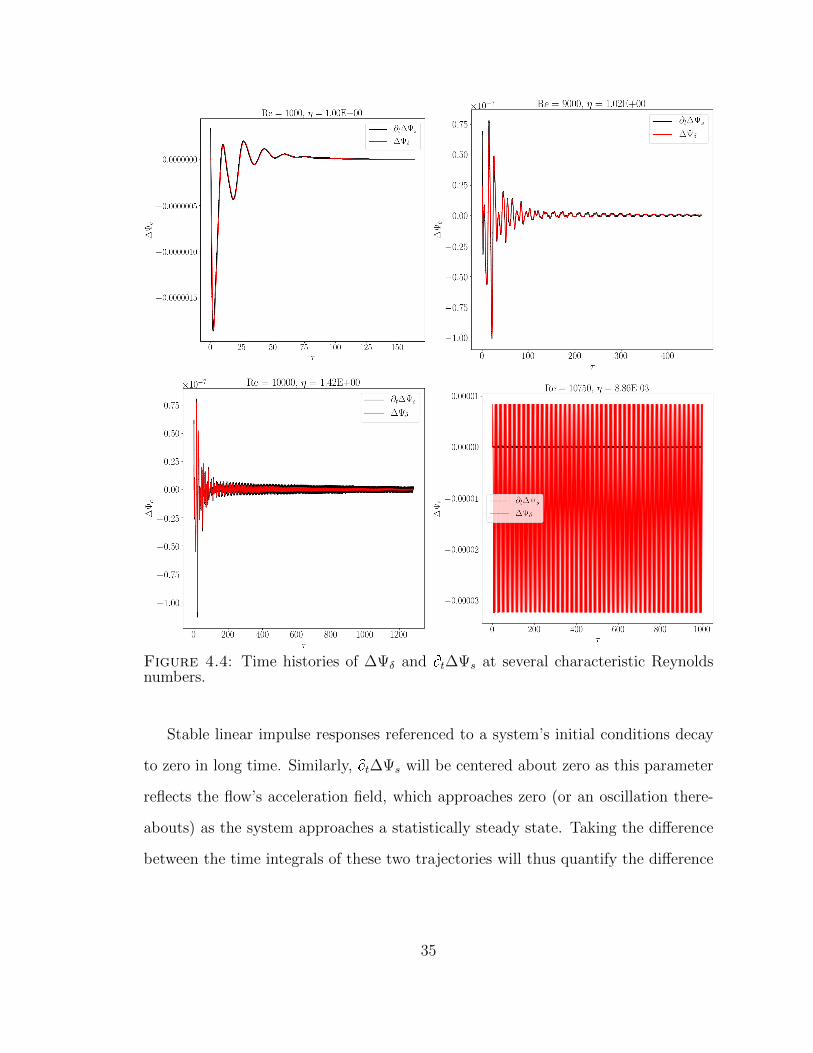
simulations: one unit impulse response and one step response. Figure 4.4 presents
∆Ψδ and Bt∆Ψs at Reynolds numbers well below, nearly at, and nearly above Recrit
for comparison.
34
Figure 4.4: Time histories of ∆Ψδ and Bt∆Ψs at several characteristic Reynoldsnumbers.
Stable linear impulse responses referenced to a system’s initial conditions decay
to zero in long time. Similarly, Bt∆Ψs will be centered about zero as this parameter
reflects the flow’s acceleration field, which approaches zero (or an oscillation there-
abouts) as the system approaches a statistically steady state. Taking the difference
between the time integrals of these two trajectories will thus quantify the difference
35
between Bt∆Ψs∆Res and ∆Ψδ. The linearity coefficient η is thus defined as
η
³τfτ0Bt∆Ψsdt
∆Res³τfτ0
∆Ψδdt
or equivalently
η ∆Ψspx, y, τf q ∆Ψspx, y, τ0q
∆Res³τfτ0
∆Ψδdt
. (4.12)
A fully linear regime would have a linearity coefficient of 1, whereas a fully nonlinear
regime would have a linearity coefficient of 0 (or very close to 0). An important
caveat to this fact is that where both trajectories are very close to zero for the entire
integration history, numerical artifacts may be magnified and yield linearity coeffi-
cients not representative of the system’s behavior. For this reason, only transient
data was used to compute linearity coefficients; in a linear system Equation 4.12
applies in the transient regime as well as the steady-state regime so this does not
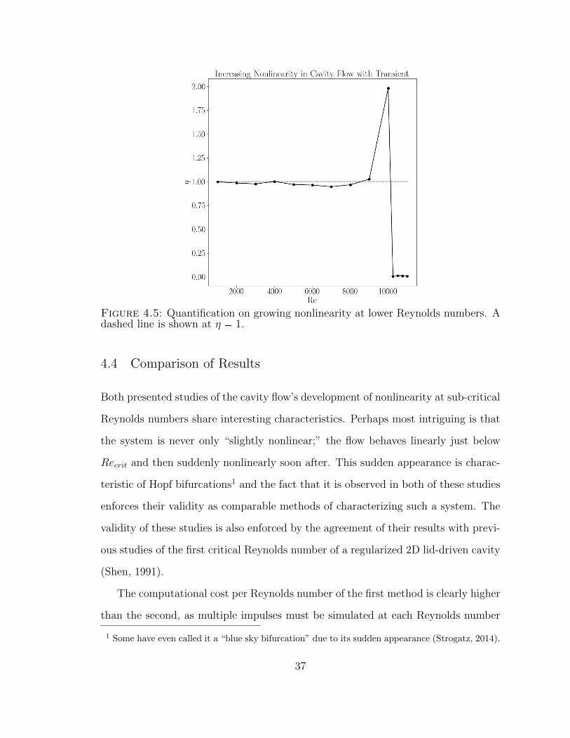
detract from the effectiveness of such a comparison. Figure 4.5 presents these trends
in η as Reynolds number increases.
The plot in Figure 4.5 identifies nearly the same critical Reynolds number as
the analysis presented in §4.2. The spike in η at Re 10, 000, followed by the
sudden low-η stabilization at Re 10, 250 and above, indicates that the critical
Reynolds number is between Re 10, 000 and Re 10, 250. The decrease in η after
Re 10, 000 is due to the fact that the limit cycle at Re 10, 000 is small enough
in amplitude to not change sign during its oscillations, where by Re 10, 250 the
limit cycle is large enough in amplitude to change sign even though it is not centered
about zero; thus, the integrals defining η become less indicative of nonlinearity soon
after large limit cycles appear.
36
Figure 4.5: Quantification on growing nonlinearity at lower Reynolds numbers. Adashed line is shown at η 1.
4.4 Comparison of Results
Both presented studies of the cavity flow’s development of nonlinearity at sub-critical
Reynolds numbers share interesting characteristics. Perhaps most intriguing is that
the system is never only “slightly nonlinear;” the flow behaves linearly just below
Recrit and then suddenly nonlinearly soon after. This sudden appearance is charac-
teristic of Hopf bifurcations1 and the fact that it is observed in both of these studies
enforces their validity as comparable methods of characterizing such a system. The
validity of these studies is also enforced by the agreement of their results with previ-
ous studies of the first critical Reynolds number of a regularized 2D lid-driven cavity
(Shen, 1991).
The computational cost per Reynolds number of the first method is clearly higher
than the second, as multiple impulses must be simulated at each Reynolds number
1 Some have even called it a “blue sky bifurcation” due to its sudden appearance (Strogatz, 2014).
37
instead of just one impulse and one step perturbation. As such, these two methods
provide benefits for different forms of trend identification. For a single Reynolds
number, the method in §4.2 provides a better data set from which the attractor
basin can be identified. Drawing conclusions across Reynolds numbers became more
subjective, as the trends identified were in part dependent on what collapsing func-
tion was selected. By contrast, the method in §4.3 provides an easier-to-produce
data set across several Reynolds numbers from which broad conclusions about the
system’s progression to nonlinearity can be drawn. As such, the method to imple-
ment depends largely on the research question at hand. If a project is focused on the
dynamics of a flow at one low Reynolds number, then the first method will provide a
better data set; if a project is instead focused on the flow’s behavior within a wider
parametric space, e.g. Reynolds number, then the second method appears to provide
comparable results for less computation.
38
5
Lyapunov Characteristic Exponents
A system’s progression to chaos is formally very difficult to identify, even for systems
much simpler than the regularized lid-driven cavity. For example, a formal identi-
fication of chaos in the Lorenz system, which is recognized as a canonical chaotic
system, was not presented for several decades after the system was originally intro-
duced (Lorenz, 1963; Mischaikow & Mrozek, 1995). To formally identify chaos, one
often must observe a system’s behavior in the limit of infinite time; this, clearly, is
not reasonable for high-dimensional systems like the lid-driven cavity.
The computation of Lyapunov characteristic exponents is a common way of de-
termining the “chaoticity” of a simulated system. In general, the characteristic expo-
nents of a nonlinear dynamical system characterize its long-time stability; character-
istic exponents greater than 0 indicate that the system is diverges from equilibrium.
For example, a system that can be modeled in part by an exponential function, e.g.
upx, tq eλt psinpxq cospxqq ,
diverges in time when λ ¡ 0.
Lyapunov characteristic exponents (LCE’s) apply this logic to chaotic systems
39
by characterizing their exponential divergence from an unperturbed path. If at least
one of the LCE’s is greater than zero, the system exponentially diverges from an
unperturbed path for an arbitrarily small perturbation and system is thus chaotic.
This quantifies the identification of chaotic system as one with extreme sensitivity
to initial conditions. Non-chaotic systems would not exponentially diverge from an
unperturbed path given any arbitrarily small perturbation; there would be realms of
stability. There are as many LCE’s as there are eigenvalues (and degrees of freedom)
for a given system, but as is the case with traditional characteristic exponents only
a single LCE must be positive to make a system chaotic. The magnitude of the
positive LCE’s indicates “how chaotic” one system is relative to another.
There are some important differences between LCE’s and the actual eigenval-
ues of the system. Perhaps most importantly for this study, the LCE’s are real,
global, averaged values. While there are many ways of computing the LCE spectrum
(Benettin et al., 1980; Wolf et al., 1985; Geist et al., 1990; Barna & Tsudo, 1993;
Tancredi et al., 2001), if the only goal is to determine whether a system is chaotic
one only needs the largest Lyapunov exponent (LLE). If the LLE is less than zero,
then the system is not chaotic. Certain methods have been developed for computing
only the LLE instead of the entire LCE spectrum because of the significantly reduced
computational cost. One such method is introduced by Sprott (2003).
Sprott’s method for computing the largest Lyapunov exponent involves spatial
and temporal averaging over many time steps where a continuously perturbed and
adjusted trajectory is compared to an unperturbed trajectory with the same initial
conditions. Sprott’s method proceeds as follows.
1. Start two trajectories A and B with initial conditions separated by some small
distance d0
2. March both trajectories in time at least one time step and compare new sepa-
40
ration d1
3. Adjust trajectory B from B1d1 to d0d1pB1 A1q. This allows for the perturbed
trajectory to remain a bounded distance from the unperturbed, or fiducial,
trajectory while still maintaining the direction of maximum expansion.
4. Compute that time step’s Lyapunov exponent λn lndnd0
∆t. In multi-DoF
systems like the cavity, this should be done at all points using a root-square
approach.
5. Iterate through steps 2-4 many times until the computed exponents converge.
6. Time-average the computed exponents to find the system’s converged largest
Lyapunov exponent.
In performing many adjustments, the system’s LCE spectrum becomes filtered
until only the largest value remains. If the largest Lyapunov exponent is positive,
then the system is chaotic. This filtering is made possible by correctly adjusting the
perturbed trajectory each time step. Sprott explains that the perturbed trajectory
can be adjusted less often than every time step, though in his words this requires
“additional bookkeeping” (Sprott, 2003). It was suggested that O p106q time steps
would be necessary for even simple chaotic systems like the Lorenz equations to yield
a converged LLE.
The details of this method’s implementation to the lid-driven cavity system is
presented below.
1. Start with the system’s steady state as computed from rest at a given Reynolds
number. Perturb the cavity by some small magnitude ε such that within the
entire cavity Ψpert Ψp1 εq. In this case, ε 0.001.
2. March both trajectories in time a certain number of time steps.
41
3. Adjust the perturbed trajectory using the expression presented above. How-
ever, as this system is computed using a second-order time-marching scheme,
the previous time-step must also be adjusted to correctly maintain the direc-
tion of maximum expansion. This was done by maintaining the same slope
between the adjusted point Bn and the previous point Bn1. Mathematically,
B1
n1 B1
n Bn Bn1 where r s1 indicates the adjusted points.
4. Compute that time step’s Lyapunov exponent λn using the expression presented
above. The root-square approach dn bpΨij Ψ0ijq2N2 was used to perform
the spatial averaging. Here, Ψ0 is the nominal trajectory and the summed
indices are over all N -by-N discrete locations in the control volume. At each
time step, dn was compared to the nominal difference in trajectories d0 bpΨ0ij 1.001Ψ0ijq2N2.
5. Repeat steps 2-4 over 106 time steps.
6. Time average the computed Lyapunov exponents λn to find the converged
largest Lyapunov exponent.
The perturbation magnitude ε was found to affect the time required for expo-
nents to converge, but not significantly affect the ultimate computed exponent or its
error margins. It was also found that the number of time steps affected the rate of
convergence more than the ultimate computed exponent or its error margins. For
brevity, the data supporting these conclusions is omitted. The computed LLE’s are
presented in Table 5.1 and Figure 5.1 for Reynolds numbers spanning the known
dynamical spectrum of the lid-driven cavity flow.
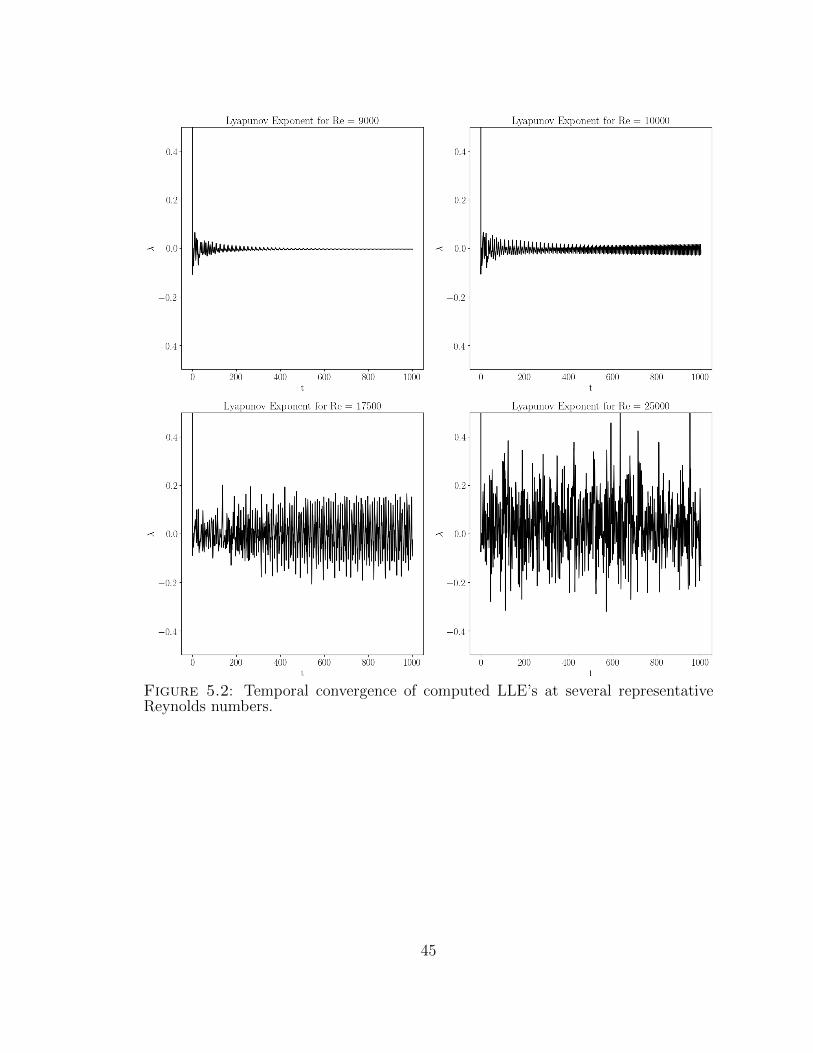
These trends, however interesting, are not meaningful without an understanding
of the LLE’s convergence. Figure 5.2 shows that the LLE’s, even in long time, did
not converge at higher Reynolds numbers; what is more, the trends identified are
42
Table 5.1: Computed LLE’s at Reynolds numbers ranging from 5, 000 to 25, 000.Error margins are not listed.
Re λ Re λ5,000 -0.0063 18,000 0.00177,000 -0.0046 18,500 0.00409,000 -0.0036 19,000 0.0012
Figure 5.1: Computed LLE’s at Reynolds numbers spanning the cavity’s dynamicalspectrum. Erro margins are not plotted.
largely invalid due to the oscillations of λn about zero with amplitudes much larger
than the time-averaged LLE’s in Table 5.1.
While these oscillations invalidate the trend identified in Table 5.1 and Figure 5.1,
they are not necessarily unexpected. Sprott’s LLE computation method is known
to have this convergence difficulty for very high-dimensional systems like the cavity
43
flow.1 Since Sprott’s relatively simple method was developed, more complex ones
have been introduced which have compute the LLE with more rigor – and much
more computational cost.
The question is thus asked: can the cavity’s Lyapunov exponents be computed
to a degree of fidelity that allows for meaningful dynamical conclusions to be drawn?
Although the formal identification of chaos in a system through the computation
of the LCE spectrum (or the associated the Kaplan-Yorke dimension) yields an ex-
traordinary amount of insight into the system’s dynamical behavior, for complex,
high-dimensional systems like a cavity flow the cost to do so is often prohibitive. As
such, less formal but more attainable methods of characterizing the cavity flow’s pro-
gression to chaos were implemented. These methods and their results are discussed
in the following chapters.
1 Appreciation is extended to Dr. H. Greenside for this insight.
44
Figure 5.2: Temporal convergence of computed LLE’s at several representativeReynolds numbers.
45
6
Higher Reynolds Number Dynamics – PoincareSub-Maps
The nonlinear dynamics present in the cavity flow above the first Hopf bifurcation will
be analyzed in two ways over the following two chapters. The qualitative changes
apparent in the flow as the Reynolds number increases will be characterized first
within the phase space and then within the power spectrum. Both studies will
observe the flow progress from periodic to quasi-periodic states, then subsequently
to chaotic, back to periodic, and finally through quasi-periodicity to chaos once again.
In the nomenclature introduced by Gollub & Benson (1980), the cavity thus exhibits
a P Ñ QP Ñ B Ñ P Ñ QP Ñ B progression to chaotic flow.
This chapter will focus on the dynamics observed with Poincare sub-maps gen-
erated from the flow’s phase space. Although the cavity flow’s true stream function
phase space would have a dimension in the dozens of thousands, for obvious reasons
this is not a realistic domain within which to study the flow’s dynamics. Rather,
as has been the case throughout this report, a representative sub-space was instead
studied. The sub-spaces observed were defined by the horizontal and vertical velocity
46
and/or acceleration components at the cavity’s center.
6.1 Phase Sub-Spaces
A system’s phase space is the domain within which all possible trajectories lie.
Within the phase space, basins of attraction influence a particular trajectory’s be-
havior. In a linear system, the phase space is one global basin of attraction in which
all trajectories are drawn to the same fixed point in long time; in a nonlinear sys-
tem, however, there can be multiple fixed points which in turn means the system’s
initial conditions determine towards where in the phase space the trajectory will
tend. For a one-dimensional oscillator whose position is defined by the variable x,
the phase-space will be two-dimensional: one axis will be x and the other will be
dxdt 9x. An important characteristic of trajectories plotted within the phase space is
that they may never intersect with each other; this would violate the uniqueness of
the governing equations’ solution for that trajectory’s specific initial and boundary
conditions. If trajectories are observed to intersect in a plotted phase space, then the
phase space must be of larger dimension than is plotted to prevent the intersection
from actually occurring.
In a discretized continuum like a simulated fluid flow, the dimension of the phase
space depends on the discretization of the volume. In this case, with the domain
being composed of a 129 129 square grid and the 2D flow being defined by the
stream function the phase space can be presented as a domain of 1292 dimensions
with each dimension being the stream function at a different location.1
For obvious reasons such a phase space was not observed. Therefore, differ-
ent reduction strategies were employed to study the system’s dynamics in a more
palatable domain. In this study, two 2D phase sub-spaces were considered at each
1 As the flow is not truly random, there is of course coupling between the stream functions atmany of these nodes. However, that coupling is not necessarily known a priori, especially at higherReynolds numbers.
47
Reynolds number: one composed of the horizontal and vertical velocity components
u and v, and one composed of the corresponding acceleration components 9u and
9v. In Figure 6.1 the flow’s trajectories are plotted within these phase sub-spaces at
three characteristically different Reynolds numbers. While these plotted trajectories
present meaningful qualitative trends, a more formal investigation can be conducted
by taking Poincare sections.
6.2 Poincare Sub-Maps
Poincare sections (more formally sub-sections as they are taken from phase sub-
spaces) were taken in these Reynolds-varying sub-spaces. These sections involve
sampling the trajectories only at certain repeating events instead of continuously.
To be effective, the event should not be directly based on the parameters defining
the phase space; for example, in this study the stream function was used to define
the events as the phase spaces were defined by velocity and acceleration components.
Two events were selected for the Poincare mapping:
Event 1 : Ψ Ψ 0 (6.1a)
Event 2 :BΨ
Bt 0 . (6.1b)
As such, four sub-maps were generated at each Reynolds number: one from velocity
components and one from acceleration components for each of these two events.
It was found that, with minimal differences, the acceleration sub-spaces presented
similar dynamical trends to the velocity sub-spaces. The two events were also found
to present similar dynamical trends. Figures 6.2 and 6.3 present all four Poincare
sub-maps at, respectively, a periodic and chaotic Reynolds number.
For brevity, only sub-maps utilizing the first event will be presented for the re-
mainder of this chapter (with the exception of Figure 6.6). The Poincare velocity
48
sub-maps adequately captured the flow’s progression through multiple bifurcations.
For example, the map at Re 15, 500 – the upper limit of what Shen (1991) studied –
shows a departure from the two-point (i.e. cleanly periodic) sub-map at Re 15, 000
(Figure 6.4), just as Shen observed. However, the next several maps do not present
a cloud that would be indicative of chaos, but instead present a complex attractor
that exists in more than the two plotted dimensions. These shapes may indicate
quasi-periodicity rather than chaos. Only at and above Re 18, 500 do the maps
present the more complex patterns indicative of a truly chaotic flow.
Increasing still further in Reynolds number, an interesting bifurcation is captured
near Re 21, 000. The flow appears to move from a chaotic pattern at Re 20, 500
to a periodic pattern, dominated by a single frequency, at Re 20, 750, and then
back to apparent chaos by Re 23, 000. Figure 6.5 presents the sub-maps in this
region of Reynolds numbers. The attractor seems to very quickly coalesce to a simple
orbit and then gradually decompose back into apparent chaos through a minuscule
quasi-periodic range. The asymmetry of this bifurcation is notable.
However clear the bifurcation near Re 21, 000 seems to be, it is not a definitive
boundary between the system’s quasi-periodic and fully chaotic Reynolds number
ranges. Bifurcations such as this can occur in the middle of a chaotic regime, sep-
arating two different, yet equally chaotic, system states. However, the bifurcation
does indicate that the system is fully chaotic by Re 23, 000; the Reynolds num-
bers between 18, 000 and 23, 000 would appear to represent a gradual transition from
quasi-periodicity to chaos.
6.3 Sub-Orbit Diagrams
While dynamically descriptive on their own, the Poincare sub-maps were also used
as the bases for sub-orbit diagrams (Figure 6.6). In these plots, all points on a given
Poincare sub-map are plotted at the same Reynolds number on the horizontal axis
49
and distributed along the vertical axis. This is done using a root sum of squares
approach for u and v or 9u and 9v, e.g.?u2 v2. The resulting diagrams for the
velocity and acceleration spaces are presented in Figure 6.6. Both figures present
the first Hopf bifurcation, the progression to quasi-periodicity near Re 15, 500,
and the dramatic bifurcation near Re 21, 000. However, the acceleration diagrams
more clearly show these events. The velocity diagrams, on the other hand, present a
stronger sense of continuity between the attractor basins across Reynolds numbers.
6.4 Progression to Chaos
The progression to chaos is apparent from both the Poincare sub-maps and the
sub-orbit diagrams. The sub-maps present a progression from two-point periodic os-
cillations, through indeterminate, non-random shapes indicative of quasi-periodicity,
to ultimately complex maps of scattered points with no discernible pattern. One
notable characteristic is the observed lack of period doubling; four distinct points
do not emerge from two, eight from four, and so on. Instead, the system exhibits
a toroidal bifurcation over a range of several thousand Reynolds numbers between
18, 000 and 23, 000. Such a bifurcation has been observed in systems including the
Lorenz equations (Sparrow, 1982).
There is, however, a limit to the dynamics apparent from these phase sub-spaces
and Poincare sub-sections. The attractor shapes apparent from the sub-maps may
not be fully realized without indeterminately long simulations in time. It is clear
from the trajectories in Figure 6.1 that the periodic attractor warps by Re 16, 500.
However, at what point does the complex but coherent attractor become formally
“strange,” as characterized by Ruelle & Takens (1971)? One cannot be sure if the
swirling trajectory at Re 25, 000 perfectly repeats itself – thereby disqualifying it
as formally chaotic – in some very, very long time. An attempt to approach these
and other questions more formally is presented in the following chapter.
50
Figure 6.1: Phase sub-spaces at periodic (top), quasi-periodic (middle), and chaotic(bottom) Reynolds numbers.
51
Figure 6.2: Four different Poincare sub-maps at a periodic Reynolds number.
52
Figure 6.3: Four different Poincare sub-maps at a chaotic Reynolds number.
53
Figure 6.4: Poincare sub-maps of Reynolds numbers just beyond what Shen studiedwhich suggest quasi-periodicity.
54
Figure 6.5: Poincare maps showing a high-Reynolds number bifurcation.
55
Figure 6.6: Sub-orbit diagrams generated from the Poincare sub-maps (velocitieson left, accelerations on right).
56
7
Higher Reynolds Number Dynamics – The PowerSpectrum
An analysis of the power spectrum supports the conclusions drawn from the Poincare
sub-maps; it also yields a better understanding of the progression from periodicity,
through quasi-periodicity, to chaos.
Following Gollub & Benson (1980) as a model for power spectrum analysis, a
similar approach was taken with the lid-driven cavity. The path to chaos is not
necessarily universal for all flows, though an analysis of the power spectrum will
be shown to yield a better understanding of a particular flow’s progression through
multiple qualitatively different states, all of which ultimately end in some form of
chaotic (i.e. what Gollub and Benson termed “non-periodic”) flow. As only one
variable (the Reynolds number) is modified in this analysis whereas Gollub and
Benson modified several (the Rayleigh and Prandtl numbers as well as system aspect
ratio), this analysis will only identify one route to chaos for the cavity.
Six representative power spectra are presented in Figure 7.1. The cavity was
observed to progress from a stable periodic state (deemed “P” following Gollub and
57
Benson’s nomenclature) to a quasi-periodic state (deemed “Q”). Following a form of
Gollub and Benson’s third path to chaos, after different forms of quasi-periodicity
present themselves the power spectrum becomes broadband (deemed “B”) and the
system is thus identified as chaotic by Re 18, 000. This is slightly lower than the
Re 18, 500 chaos milestone identified in the Poincare sub-maps, but in studying this
power spectrum one observes that, while the presence of noise (and thus aperiodicity)
is clear, the system is still largely dominated by quasi-periodic peaks; this would
explain why a discernible pattern was still present in the Poincare sub-maps at this
aperiodic Reynolds number. This observation supports the conclusion that Poincare
sub-maps require much longer time histories than what is presented to definitively
characterize quasi-periodicity versus chaos. The lack of a broadband pattern in a
power spectrum with many incommensurate frequencies and their harmonics, as is
the case at Re 19, 000, strongly suggests quasi-periodicity over chaos. The sudden
reappearance of a periodic state near Re 21, 000 is just as apparent in the power
spectra, as is the clear movement back through quasi-periodicity to chaos at higher
Reynolds numbers.
There are some larger peaks even amongst the broadband noise. However, as
stated by Gollub and Benson, “[i]f the velocity spectrum contains any broadband
noise, the motion is non-periodic...even if relatively sharp spectral peaks are also
present” (Gollub & Benson, 1980).
7.1 Quasi-Periodic Spectrum Reduction Algorithm
However clean-cut the periodic and aperiodic power spectra may be, it is difficult to
analyze formally the quasi-periodic spectra. The “trees in a forest” appearance of
a quasi-periodic power spectrum qualitatively differs from the “needles in a bush”
appearance of a broadband spectrum, but – to continue the analogy – as more trees
populate the forest it becomes harder to identify the main species, or less figuratively
58
Figure 7.1: Power spectra at representative Reynolds numbers.
the dominant frequencies. An attempt at objectively studying these intermediate,
quasi-periodic states is presented in the following sections. The results will include
a novel perspective on how quasi-periodicity can become chaos.
An algorithm was developed to identify quasi-periodic patterns in power spectra.
Each power spectrum is treated separately; as such, any resulting trends across the
several power spectra are more objectively identified. The algorithm is presented in
Algorithm 1.
This algorithm was applied to power spectra at Reynolds numbers ranging from
59
Algorithm 1 Given a vector of frequencies for power spectrum peaks which is sortedwith the largest peak’s frequency first and truncated to peaks of magnitude largerthan Smin, this algorithm returns a vector of three present frequencies to which allothers present can be reduced or a vector of r1,1,1s if such reduction is notpossible. The peak truncation was inspired by the work of Wiebe and Virgin (Wiebe& Virgin, 2012).
if there are 3 or fewer ω’s thenreturn [all ω’s] algorithm requires more than 3 ω’s
end if
for all combinations of ωi, ωj, ωk do biased to larger peaksEnsure: ωi ωj ωkfor all input frequencies ωm do
ifmaxpωijk,ωmq
minpωijk,ωmqis an integer then
mark ωm as passed harmonics all foundelse if pωi qωj rωk ωm@ p, q, r P r2, 2s Z then
mark ωm as passed sums of first harmonics foundend if
end for
if all input frequencies marked as passed thenreturn rωi, ωj, ωks quasi-periodic frequencies found
end ifend for
return r1, 1, 1s no quasi-periodic frequencies found
Re 10, 250, the first with a non-negligible frequency peak, up to the maximum
Reynolds number observed in this study: Re 25, 000. For consistency, all cases
were run to τf 5, 000 with the power spectrum being generated from the last 4,000
dimensionless time units (4 106 time steps). Thus, all studied power spectra had
a frequency resolution of ∆ω 0.0025. The results are presented in Table 7.1 and
analyzed in the following sections. The peak truncation was set to Smin 105.
All frequencies presented at Re 21, 500 remained relatively dominant until Re 25, 000.
It was observed that a broadband power spectrum was reduced to quasi-periodicity
at Re 18, 000; this is because the broadband pattern, presented in Figure 7.2, ex-
isted largely below Smin 105 and was therefore not observed for reduction. (26
present frequencies were captured at this Reynolds number.) The mechanics by
60
Table 7.1: Tabulated results from quasi-periodicity algorithm. Reynolds numberswith broadband power spectra are denoted by BRe. Reynolds numbers that werenot quasi-periodic according to the algorithm are denoted by Re.
which these different frequencies appear and interact will be discussed in subsequent
sections.
7.2 Definition of Terms
Several terms will be introduced before continuing the discussion of the frequency
spectra. This is done in the hope that such a formal definition of terms will limit
the amount of ambiguity in the analyses presented below.
A present frequency is one that corresponds to a peak in the power spectrum.
A dominant frequency is one that appears to control the power spectrum.
For example, the presented reduction algorithm attempts to resolve multi-
61
Figure 7.2: Broadband power spectrum at Re 18, 000 which still exhibits domi-nant quasiperiodic characteristics.
ple present frequencies into three dominant frequencies. Dominant frequen-
cies must be formally incommensurate with one another. Using Gollub and
Benson’s characterization, the ratios between dominant frequencies must vary
within the parameter space (Gollub & Benson, 1980).
A novel frequency is a dominant frequency that cannot be explained by en-
trainment, shredding, or simple interaction between other dominant frequen-
cies. For example, 0.098 is a novel frequency that appears at Re 15, 500 as
presented in Tables 7.1 and 7.2.
A resonating frequency is one that the system appears to be biased to-
wards. While a resonating frequency does not necessarily elicit the response of
a “resonant frequency” as defined in classical dynamics, it does appear to be
62
an energy sink (see discussion below) within the spectrum. Natural frequencies
are often resonating frequencies and resonating frequencies are often dominant
frequencies.
Frequency entrainment is a concept discussed by Gollub & Benson (1979,
1980) by which multiple dominant frequencies may temporarily interact in such
a way that the observed behavior is of a momentarily common harmonic.
Frequency shredding occurs when a clean peak in the power spectrum breaks
down into a collection of nearby frequencies, thus dramatically increasing the
likelihood of harmonic interaction elsewhere in the power spectrum.
Power capacity is the power spectrum magnitude for a frequency above which
that frequency may shred to reduce its contained power.
These concepts will be discussed in detail in subsequent sections. A more com-
prehensive form of Table 7.1 is presented near the end of this chapter and will include
patterns identified with these concepts.
7.3 Frequency Entrainment
Several dominant frequencies seem to appear and disappear as the Reynolds number
increases. By Re 25, 000, the flow is chaotic with both a broadband power spec-
trum and a complex Poincare sub-map. The system changes qualitatively between
periodic, quasi-periodic, and non-periodic (i.e. chaotic) states, and therefore tech-
nically goes through multiple bifurcations on its way to chaos; identified patterns,
however, suggest that the changes are both reconcilable and potentially predictable.
Many of the dominant frequencies at any Reynolds number can be explained by
simple interactions between the dominant frequencies at the previous Reynolds num-
ber. (Table 7.2 presents some of these combinations in brackets between Reynolds
63
numbers.) In fact, most of the dominant frequencies appear to arise from various
interactions between (e.g. additive combinations of) previous dominant frequencies
and their harmonics. This suggests that an analysis of frequency combinations at a
given Reynolds number could predict the behavior at the following Reynolds num-
ber; frequencies that can result most often from combinations of current frequencies
are more likely to appear at higher Reynolds numbers.
For example, the power spectrum presents a broadband pattern at Re 20, 500
whose largest frequency peaks exist at ω 0.237, 0.057, 0.090, 0.204, and 0.034.
The only dominant frequency observed at Re 20, 750 is at ω 0.236. This fre-
quency was present at the last observed Reynolds number, but is also a combination
of 0.204 0.034 and 0.057 2 0.090 when the independent drifting of all dom-
inant frequencies is accounted for. In this way, the broadband power spectrum at
Re 20, 500 briefly became a periodic power spectrum at Re 20, 750 because
of frequency entrainment. As the resonating frequencies continued to drift as the
Reynolds number further increased, the entrainment passed and the system became
broadband once again after an intermediate lapse to quasi-periodicity.
Certain resonating frequencies also appear to be the most common within the
system. Frequencies of approximately 0.054, 0.096, and 0.036 appeared to resonate in
this system; however, many dominant frequency combinations yield the original novel
frequency of 0.165 when the observed downward drift of this first novel frequency is
considered. As such, 0.165 may also be considered a resonating frequency when one
considers its shredding (see below) at a relatively low Reynolds number.
The concept of frequency entrainment (Gollub & Benson, 1979, 1980) explains
many of the dominant frequencies observed at higher Reynolds numbers. Because
these momentary lapses in aperiodicity are so readily explained by frequency en-
trainment, it is debatable whether these qualitative changes in behavior are formal
bifurcations. While the nature of the system momentarily changes, it is more due
64
to a serendipitous interaction of multiple dominant frequencies than due to a novel
appearance or disappearance of a frequency. By this reasoning, the only observed
bifurcation after the first is at Re 15, 500, where the novel frequency ω 0.098
appears out of apparently nowhere. This behavior at Re 15, 500 may have been
what led Shen (1991) to conclude a certain degree of “turbulence” at this and higher
Reynolds numbers.
7.4 Frequency Shredding
Frequency entrainment alone cannot explain the appearance of many other frequen-
cies as the Reynolds number increases. Keeping in mind the apparent interacting
nature of developing frequencies, a new concept is now introduced, “frequency shred-
ding,” that can help to explain more specifically how the interactions appear to hap-
pen. Recall that frequency shredding is defined as follows: an event which occurs
when a clean peak in the power spectrum breaks down into a collection of nearby
frequencies, thus dramatically increasing the likelihood of harmonic interaction else-
where in the power spectrum. In essence, a shredded frequency spreads its energy
over a range of nearby frequencies that then allows for many more potential interac-
tions, which often results in the dominant frequencies moving around the spectrum.
Symbolically, shredding of a frequency ω can be noted as Spωq.An example of shredding is observed between Re 18, 000 and Re 18, 500,
where ω 0.057 shreds and transfers some of its energy to ω 0.062. As observed
in Figure 7.3, the 0.057 peak spreads to include 0.062, which then itself grows in
amplitude.
The behavior observed in Figure 7.3 can not be explained by frequency entrain-
ment; the creation of more frequencies from fewer is in some ways the inverse of
entrainment, where fewer frequencies become dominant from within a larger selec-
tion. A combination of entrainment and shredding, however, appears to explain
65
Figure 7.3: Intermediate shredding of 0.057 near Re 18, 000. A dotted line isincluded at the original peak location for reference.
almost all of the dynamics presented in Table 7.1.
Frequency shredding, like entrainment, appears to have its own nuances. The
outcomes of frequency shredding were observed to be threefold:
1. Spωq Ñ ω, ω δ: intermediate shredding, where a resonating frequency (one
that is the result of other frequencies already present) that is very nearby the
original peak frequency (with small distance δ from the original frequency)
becomes excited, drawing energy away from the original peak frequency;
2. Spωq Ñ ωm, ωn: destructive shredding, where the shredding frequency band
sends all of its energy to two or more incommensurate frequencies elsewhere in
the frequency spectrum; and
3. Spωq Ñ ω, ωm, ωn: constructive shredding, where the shredding frequency
only sends some of its energy to two or more incommensurate frequencies else-
where in the spectrum.
When a frequency shreds, the energy contained in the shredded peak attempts
to move to other frequencies. If the shredding appears near a resonating frequency,
then that frequency will likely draw at least some of the shredded energy. If this is
not the case, then the shredded energy will tend towards dominant and/or resonating
frequencies from which the original shredded frequency can be derived. Using the
66
above notation, ωm and ωn are incommensurate frequencies that can easily interact
to yield the original shredded frequency. Intermediate shredding can explain the
dynamics observed in Figure 7.3.
An example of destructive shredding is observed between Re 12, 000 and Re 13, 000. The only frequency dominant at Re 12, 000 shreds into two dominant
frequencies at Re 13, 000. As is shown in the top of Figure 7.4, the stream
function at the cavity center appears to stabilize in a quasi-periodic limit cycle within
the first 4,000 dimensionless time units. However, as this Reynolds number was run
to τf,impulse 5, 000 for consistent resolution in the power spectrum, a secondary
transient was observed that did not stabilize by the end of the first simulation (to
τf,impulse 5, 000). As such, the flow was simulated to τf,impulse 10, 000 to observe
what happened; ultimately the flow stabilized in an alternate limit cycle.
The power spectra for the different stages of this time history are presented as
well in Figure 7.4. It is clear that the system went from a quasi-periodic state back
to a periodic state, where the final frequency was approximately 0.161: the same
frequency as was observed at Re 12, 000. What is more, taking the difference be-
tween the dominant quasi-periodic frequencies yielded this later periodic frequency:
0.196 0.035 0.161.
The following conclusion can thus be drawn. The flow at Re 13, 000 has
enough energy to destructively shred the original frequency into two incommensurate
components, but does not have enough energy for these two frequencies to be stable
in long time. Thus, in long time each of these two frequencies themselves shred,
again destructively, and the energy is transferred back to the original state. It
is hypothesized that if the simulation was run for very, very long times, the flow
would oscillate between these two states. However, this may not be the case as the
energy input from the impulse perturbation may have been the cause for the initial
shredding.
67
An example of constructive shredding is observed between Re 15, 000 and
Re 15, 500. Here, the dominant frequency 0.156 constructively shreds to pass some
of its energy to the resonating frequency 0.040. It also happens that at Re 15, 500 a
novel frequency appears as well; it is possible that this novel frequency’s appearance
destabilized the original dominant frequency enough to cause it to constructively
shred, but not enough to destructively shred. Figure 7.5 shows this constructive
shredding.
It is worth noting that one of the presented power spectra in the paper by Peng
et al. (2003) presents frequency shredding. The power spectrum presented in Figure
6 is a shredded power spectrum at Re 10, 300 which is observed between two non-
shredded power spectra at Re 10, 200 and 10, 400. What is more, the shredding
appears to be constructive because the original frequency of 0.5 is still dominant (but
no longer exclusively so) after the shredding occurs.
7.5 Power Capacity
The concept of “power capacity” is now introduced in an attempt to explain why
shredding occurs and also when and where it occurs. Recall that power capacity
is defined as follows: the power spectrum magnitude for a certain frequency above
which that frequency shreds to reduce its contained power. In other words, the
power capacity of a given frequency determines how much energy can be contained
within that frequency; if more energy is put into that particular frequency, then the
frequency will shred, i.e. de-stabilize, to allow energy to escape that frequency. If a
dominant frequency is below its power capacity, it will resonate and collect energy
from other frequencies attempting to lose energy.
The three examples of shredding presented above will be discussed in the context
of power capacity. Observing first the intermediate shredding in Figure 7.3, one can
conclude that the power capacity of ω 0.057 appears to be approximately 2103.
68
This is because when more energy is put into this frequency, which is accomplished
by increasing the Reynolds number, it shreds and its stored power reduces to closer to
1 103 at Re 18, 000. As the broadband spectrum and the resonating ω 0.062
absorb the energy, ω 0.057 remains well below its power capacity.
The destructive shredding observed in Figure 7.4 can also be explained using
the concept of power capacity. The destructive shredding of ω 0.161 causes this
frequency to pass all of its energy to the two frequencies that are dominant in the
early limit cycle at Re 13, 000: 0.196 and 0.035. However, this caused too much
energy to be given to both of these resonating frequencies; at Re 13, 000, the
two dominant frequencies are both over their power capacity. Therefore, they each
shred and pass their energy back to the still resonating frequency ω 0.161, which
ultimately contains as much energy as it had at Re 12, 000 when it was stable.
The power capacity of ω 0.156 is observed from Figure 7.5 to be approximately
1 103. This is because this amount of contained power is in this frequency both
before and after it constructively shreds. This indicates that when more energy is
added to this frequency, it shreds to remove the excess, but is able to retain most
of the energy that it holds, thus keeping it near its power capacity. A construc-
tively shredding frequency therefore seems to resonate more strongly, because when
it shreds to lower its contained power it is resonating strongly enough that, once
below its power capacity, the frequency can retain much of its energy.
Applying the concepts of frequency entrainment, frequency shredding, and power
capacity to the trends identified with the quasi-periodicity algorithm allows for all
observed changes in behavior above Re 15, 500 to be rationalized. A more complete
version of Table 7.1 is presented in Table 7.2. Observed frequencies that were either
dominant in a broadband spectrum or clear peaks only present below the algorithm’s
peak truncation are included in parentheses for dynamical completeness. Readers
should note that only one novel frequency after the first Hopf bifurcation is now
69
present. Even through the broadband states, shredding and basic harmonic interac-
tions can offer an explanation as to how and why the different dominant frequencies
appear and disappear.
70
Table 7.2: Dominant frequency progression table. Reynolds numbers with broadbandpower spectra are denoted by BRe. Reynolds numbers that were not quasi-periodicaccording to the algorithm are denoted by Re. Frequencies in parentheses werepresent by inspection (or of large magnitude in broadband spectra) and includedfor dynamical completeness but were not captured by the algorithm. Results ofconstructive and destructive frequency shredding from the nth column are denotedby Spωnq and Spωnq respectively. Intermediate shredding is denoted by Spωnq.The interactions between dominant frequencies are presented in brackets where ap-plicable; additional brackets were not included for brevity. Novel frequencies areemboldened when they first appear.
Ó Spω5q Spω5q Ó rω1 ω2s Ó Spω2qB18,500 (0.246) (0.057) (0.094) (0.208) (0.188) (0.037) (.062)
rω3 ω2sÓ rω1 ω4s rω53s
19,000 0.054 r2ω2 0.036 0.063Ó rω6 ω7s ω6 ω7s Spω7q Ó Ó
B19,500 (0.053) (0.099) (0.206) (0.071) (0.036) (0.064)Ó Ó Ó Ó Ó Ó
B20,000 (0.051) (0.098) (0.205) (0.070) (0.035) (0.064)rω4 ω6s Ó Ó Ó Ó Ó Ó
B20,250 (0.239) (0.051) (0.098) (0.204) (0.072) (0.034) (0.069)Ó Ó rω3 ω7 ω5s Ó Ó
B20,500 (0.237) (0.057) (0.090) (0.204) (0.034)r2ω3 ω2srω4 ω6s Ó
20,750 0.236 (0.051)Ó
21,000 0.234Ó Spω1q Spω1q
21,250 0.232 0.031 0.069Spω1q Spω1q
Ó rω6 ω7s2 rω6 ω7s rω1 ω6s rω1 ω6 ω7s Ó ÓB21,500 (0.231) (0.050) (0.099) (0.201) (0.132) (0.030) (0.066)
Ó Ó Ó Ó Ó Ó Ó
71
Figure 7.4: The destructive but unsustainable shredding at Re 13, 000. A dottedline is included at the original peak location for reference.
72
Figure 7.5: Constructive shredding near Re 15, 500. A dotted line is includedat the original peak location for reference.
73
8
Conclusion
The regularized two-dimensional lid-driven cavity has been analyzed and its behavior
characterized from its low-Reynolds number monotonically stable states through to
its high-Reynolds number chaotic states. The first critical Reynolds number, iden-
tified near Re 10, 250, was the observable demarcation between stable-linear and
nonlinear flow behavior. It was observed that the approximately linear component of
the node’s attractor basin below the first critical Reynolds number did not noticeably
shrink until very close to the first critical Reynolds number.
The nonlinear flows observed above Re 10, 250 were characterized using a
combination of new and existing methods. It was deemed infeasible to compute the
Lyapunov characteristic exponent spectrum, or even the largest Lyapunov exponent,
in a system with such complexity. Poincare sub-maps and power spectrum analyses
each indicated that the flow qualitatively changed near Re 15, 500, where the
system seemed to transition from a periodic to a quasi-periodic state even for long
time. This Reynolds number is also where a novel frequency appeared, indicating
that it may be considered the cavity’s second critical Reynolds number.
The concepts of frequency shredding and power capacity were introduced in an
74
effort to explain how the flow evolved beyond the second critical Reynolds number.
With the concepts of frequency entrainment, frequency shredding, and power capac-
ity, the resulting explanations seem to apply equally well across the range of higher
Reynolds numbers that were studied. Although these concepts can explain the flow’s
behavior, it is not yet clear if (or to what degree) these changes can be predicted.
A more mathematically robust development of these concepts will be necessary for
such predictions.
While the author has consciously avoided the word “turbulence” in this paper,
it is possible that these concepts will provide a new perspective on energy transfer
within turbulent fields. The flow’s energy may be understood to be transferred be-
tween and among different frequencies, which each may correlate to different spatial
scales or coherent structures that Richardson (Richardson, 1920) and many others
(Kolmogorov, 1962, 1991; Lumley, 1967) have studied. This in turn may yield new
understanding of turbulent convection.
75
Appendix A
Derivation of the Viscous Incompressible VorticityEquation
Taking the curl of the Navier-Stokes equations yields
B~uBt p~u ∇q ~u 1
ρ∇P ν∇2~u
∇ B~uBt ∇ p~u ∇q ~u ∇ 1
ρ∇P ∇ ν∇2~u . (A.1)
The vorticity ~ω ∇~u appears throughout this equation, where the individual terms
simplify as follows. The first term, due to the independence of the cross product and
the time derivative, can be written as
∇ B~uBt
B p∇ ~uqBt B~ω
Bt . (A.2a)
The viscous term, like the temporal term, simplifies as follows.
∇ ν∇2~u
ν∇2 p∇ ~uq ν∇2~ω . (A.2b)
76
The pressure term vanishes for incompressible flow1 because the cross product of the
gradient of a scalar function is identically zero.
∇ 1
ρ∇P ∇∇
P
ρ
0 (A.2c)
The convective term can be rearranged as follows, applying the vector identity
∇ p~a ∇q~a ∇
1
2∇ p~a ~aq ~a∇ ~a
as well as the same vector identity that was applied to the pressure term in the
process.
∇ p~u ∇q ~u ∇
1
2∇ p~u ~uq ~u ~ω
∇ ~u ~ω
p~u ∇q ~ω p~ω ∇q ~u ~ω p∇ ~uq .
From mass conservation for incompressible flow, ∇ ~u 0, the convective term
becomes
∇ p~u ∇q ~u p~u ∇q ~ω p~ω ∇q ~u . (A.2d)
Recombining Equations A.2 yields this version of the vorticity equation in its final
form:
B~ωBt p~u ∇q ~ω p~ω ∇q ~u ν∇2~ω . (A.3)
1 Technically, the pressure term will always vanish but a density term would remain without theassumption of incompressibility.
77
Appendix B
Details of the Computational Model
1The NS equations in 2D are:
BBtp∇
2Ψq BΨ
ByBBxp∇
2Ψq BΨ
BxBBy p∇
2Ψq ν∇4Ψ (B.1)
where Ψpx, y, tq is the stream function, ∇
BBx1, . . . , B
Bxn
, ∇2 ∇ ∇, and ∇4
∇2∇2 is the biharmonic operator. Replacing Ψpx, y, tq rΨpx, y, tq Ωpx, yq where
Ω satisfies the Dirichlet boundary conditions, one obtains
BBtp∇
2rΨq BΨ
ByBBxp∇
2Ψq BΨ
BxBBy p∇
2Ψq ν∇4Ψ (B.2)
since BBtp∇2Ωq 0 by definition.
1 This appendix was prepared by M. Balajewicz.
78
B.1 Discretization
The domain px, yq P r1, 1sr1, 1s is discretized pseudo-spectrally using Chebyshev
polynomials. Thus, one can write:
BijθBxiByj DiθDT j (B.3)
where D P RNN is the differentiation matrix and θptq P RNN is the semi-discretization
of a function θpx, y, tq.
B.2 Semi-implicit 2BDF
2BDF gives:
BBtθpx, y, tq
ttn
BBtθptq
ttn
3θn1 4θn 1θn1
2∆t, (B.4)
thus
BBtp∇
2rΨq BBtD2rΨ rΨDT 2
(B.5a)
1
2∆t
3D2rΨn1 rΨn1DT 2
4
D2rΨn rΨnDT 2
D2rΨn1 rΨn1DT 2
.
(B.5b)
As before, the nonlinear convection terms are treated explicitly while the diffusion
term is treated semi-implicitly. This gives the Lyapunov equation:
ArΨn1 rΨn1AT Qn 0 (B.6)
where
A 3
2∆tD2 νD4 (B.7)
79
and
Q 4
2∆t
D2rΨn rΨnDT 2
1
2∆t
D2rΨn1 rΨn1DT 2
nDTd
DDn2 n DT 2
pDΨnq d
Dn2 n DT 2
DT
ν
D4 2Dn2
DT 2 DT 4
(B.8)
where d is the Hadamard product.
80
Bibliography
Andrade, E. N. da C. & Dodd, C. 1946 The Effect of An Electric Field onthe Viscosity of Liquids. Proceedings of the Royal Society of London. Series A,Mathematical and Physical Sciences 187 (1010), 296–337.
Balajewicz, Maciej J., Dowell, Earl H. & Noack, Bernd R. 2013 Low-dimensional modelling of high-Reynolds-number shear flows incorporating con-straints from the Navier-Stokes equation. Journal of Fluid Mechanics 729, 285–308.
Barna, Gyorgy & Tsudo, Ichiro 1993 A new method for computing Lyapunovexponents. Physics Letters A 175 (6), 421–427.
Benettin, Giancarlo, Galgani, Luigi, Giorgilli, Antonio & Strelcyn,Jean-Marie 1980 Lyapunov Characteristic Exponents for smooth dynamical sys-tems and for hamiltonian systems; a method for computing all of them. Part 2:Numerical Application. Meccanica 15 (1), 21–30.
Chien, W.-L, Rising, H & Ottino, J M 1986 Laminar mixing and chaoticmixing in several cavity flows. J . Fluid Mech 170, 355–377.
Clercx, H. J. H. & van Heijst, G. J. F. 2009 Two-Dimensional NavierStokesTurbulence in Bounded Domains. Applied Mechanics Reviews 62 (2), 020802.
Deshpande, MD & Shankar, PN 1994a Transitional and turbulent flow in athree-dimensional cavity. Natl. Aerosp. Lab. Doc. PD CF .
Deshpande, M. D. & Shankar, P. N. 1994b Direct numerical simulation of acomplex turbulent flow. Current Science 66 (10), 767–770.
Geist, Karlheinz, Parlitz, Ulrich & Lauterborn, Werner 1990 Com-parison of Different Methods for Computing Lyapunov Exponents. Progress ofTheoretical Physics A38 (5), 1157.
Gollub, J. P. & Benson, S. V. 1979 Phase Locking in the Oscillations Leading toTurbulence. In Pattern Formation by Dynamic Systems and Pattern Recognition(ed. Hermann Haken), pp. 74–80. Schloß Elmau: Springer.
81
Gollub, J. P. & Benson, S. V. 1980 Many routes to turbulent convection. Jour-nal of Fluid Mechanics 100 (03).
Gollub, J. P. & Swinney, Harry L. 1975 Onset of Turbulence in a RotatingFluid. Physical Review Letters 35 (14), 927–930.
Hopf, Eberhard 1948 A mathematical example displaying features of turbulence.Communications on Pure and Applied Mathematics 1 (4), 303–322.
Kelley, Douglas H. & Ouellette, Nicholas T. 2011 Onset of three-dimensionality in electromagnetically driven thin-layer flows. Physics of Fluids23 (4).
Kolmogorov, A. N. 1962 A refinement of previous hypotheses concerning thelocal structure of turbulence in a viscous incompressible fluid at high Reynoldsnumber. Journal of Fluid Mechanics 13 (01), 82–85.
Kolmogorov, A. N. 1991 Dissipation of Energy in the Locally Isotropic Tur-bulence. Proceedings of the Royal Society of London: Mathematical and PhysicalSciences 434 (1890), 15–17.
Koseff, J. R. & Street, R. L. 1984a On End Wall Effects in a Lid-Driven CavityFlow. Journal of Fluids Engineering 106 (4), 385.
Koseff, J. R. & Street, R. L. 1984b The Lid-Driven Cavity Flow: A Synthesis ofQualitative and Quantitative Observations. Journal of Fluids Engineering 106 (4),390.
Landau, Lev D. 1944 On the Problem of Turbulence. Dokl. Akad. Nauk SSSR44 (8), 339–349.
Lorenz, Edward N. 1963 Deterministic Nonperiodic Flow. Journal of the Atmo-spheric Sciences 20 (2), 130–141.
Lumley, John L. 1967 The Structure of Inhomogeneous Turbulent Flows. Atmo-spheric Turbulence and Radio Wave Propagation pp. 166–178.
Mischaikow, Konstantin & Mrozek, Marian 1995 Chaos in the Lorenz equa-tions: a computer-assisted proof. Bulletin of the American Mathematical Society32, 66–72.
Monaghan, J. J. & Kajtar, J. B. 2014 Leonardo da Vinci’s turbulent tank intwo dimensions. European Journal of Mechanics - B/Fluids 44, 1–9.
Peng, Yih-Ferng, Shiau, Yuo-Hsien & Hwang, Robert R. 2003 Transitionin a 2-D lid-driven cavity flow. Computers & Fluids 32 (3), 337–352.
Pope, Stephen B. 2000 Turbulent Flows . Cambridge University Press.
82
Prasad, Ajay K. & Koseff, Jeffrey R. 1989 Reynolds number and endwalleffects on a liddriven cavity flow. Physics of Fluids A: Fluid Dynamics 1 (2),208–218.
Richardson, L. F. 1920 The supply of energy from and to atmospheric eddies.Proceedings of the Royal Society London 97 (686), 345–373.
Ruelle, David & Takens, Floris 1971 On the nature of turbulence. Communi-cations in Mathematical Physics 20 (3), 167–192.
Shankar, P. N. & Deshpande, M. D. 2000 Fluid Mechanics in the Driven Cavity.Annual Review of Fluid Mechanics 32, 93–136.
Shen, Jie 1991 Hopf bifurcation of the unsteady regularized driven cavity flow.Journal of Computational Physics 95 (1), 228–245.
Sparrow, Colin 1982 The Lorenz equations: bifurcations, chaos, and strange at-tractors , , vol. 41. Springer Science & Business Media.
Sprott, Julien C. 2003 Chaos and Time Series Analysis . Oxford University Press.
Stremler, Mark A. & Chen, Jie 2007 Generating topological chaos in lid-drivencavity flow. Physics of Fluids 19 (10).
Strogatz, Steven H. 2014 Nonlinear Dynamics and Chaos: With Applicationsto Physics, Biology, Chemistry, and Engineering , 2nd edn. Westview Press.
Tancredi, G., Sanchez, A. & Roig, F. 2001 A Comparison between Methodsto Compute Lyapunov Exponents. The Astronomical Journal 121 (2), 1171–1179.
Tennekes, H. & Lumley, John L. 1972 A First Course in Turbulence. MITPress.
Verstappen, R, Wissink, J.G, Cazemier, W & Veldman, A.E.P 1994 Di-rect numerical simulations of turbulent flow in a driven cavity. Future GenerationComputer Systems 10 (2-3), 345–350.
Wiebe, R. & Virgin, L. N. 2012 A heuristic method for identifying chaos from fre-quency content. Chaos: An Interdisciplinary Journal of Nonlinear Science 22 (1).
Wolf, Alan, Swift, Jack B., Swinney, Harry L. & Vastano, John 1985Determining Lyapunov exponents from a time series. Physica D: Nonlinear Phe-nomena 16 (3), 285–317.