73
SAS/OR ® 14.1 User’s Guide: Mathematical Programming The Linear Programming Solver
SAS/OR® 14.1 User’s Guide:Mathematical ProgrammingThe Linear ProgrammingSolver
This document is an individual chapter from SAS/OR® 14.1 User’s Guide: Mathematical Programming.
The correct bibliographic citation for this manual is as follows: SAS Institute Inc. 2015. SAS/OR® 14.1 User’s Guide: MathematicalProgramming. Cary, NC: SAS Institute Inc.
SAS/OR® 14.1 User’s Guide: Mathematical Programming
Copyright © 2015, SAS Institute Inc., Cary, NC, USA
All Rights Reserved. Produced in the United States of America.
For a hard-copy book: No part of this publication may be reproduced, stored in a retrieval system, or transmitted, in any form or byany means, electronic, mechanical, photocopying, or otherwise, without the prior written permission of the publisher, SAS InstituteInc.
For a web download or e-book: Your use of this publication shall be governed by the terms established by the vendor at the timeyou acquire this publication.
The scanning, uploading, and distribution of this book via the Internet or any other means without the permission of the publisher isillegal and punishable by law. Please purchase only authorized electronic editions and do not participate in or encourage electronicpiracy of copyrighted materials. Your support of others’ rights is appreciated.
U.S. Government License Rights; Restricted Rights: The Software and its documentation is commercial computer softwaredeveloped at private expense and is provided with RESTRICTED RIGHTS to the United States Government. Use, duplication, ordisclosure of the Software by the United States Government is subject to the license terms of this Agreement pursuant to, asapplicable, FAR 12.212, DFAR 227.7202-1(a), DFAR 227.7202-3(a), and DFAR 227.7202-4, and, to the extent required under U.S.federal law, the minimum restricted rights as set out in FAR 52.227-19 (DEC 2007). If FAR 52.227-19 is applicable, this provisionserves as notice under clause (c) thereof and no other notice is required to be affixed to the Software or documentation. TheGovernment’s rights in Software and documentation shall be only those set forth in this Agreement.
SAS Institute Inc., SAS Campus Drive, Cary, NC 27513-2414
July 2015
SAS® and all other SAS Institute Inc. product or service names are registered trademarks or trademarks of SAS Institute Inc. in theUSA and other countries. ® indicates USA registration.
Other brand and product names are trademarks of their respective companies.
Chapter 7
The Linear Programming Solver
ContentsOverview: LP Solver . . . . . . . . . . . . . . . . . . . . . . . . . . . . . . . . . . . . . . 256Getting Started: LP Solver . . . . . . . . . . . . . . . . . . . . . . . . . . . . . . . . . . . 256Syntax: LP Solver . . . . . . . . . . . . . . . . . . . . . . . . . . . . . . . . . . . . . . . 259
Functional Summary . . . . . . . . . . . . . . . . . . . . . . . . . . . . . . . . . . . 259LP Solver Options . . . . . . . . . . . . . . . . . . . . . . . . . . . . . . . . . . . . 260
Details: LP Solver . . . . . . . . . . . . . . . . . . . . . . . . . . . . . . . . . . . . . . . 266Presolve . . . . . . . . . . . . . . . . . . . . . . . . . . . . . . . . . . . . . . . . . 266Pricing Strategies for the Primal and Dual Simplex Algorithms . . . . . . . . . . . . 266The Network Simplex Algorithm . . . . . . . . . . . . . . . . . . . . . . . . . . . . 266The Interior Point Algorithm . . . . . . . . . . . . . . . . . . . . . . . . . . . . . . . 267Iteration Log for the Primal and Dual Simplex Algorithms . . . . . . . . . . . . . . . 269Iteration Log for the Network Simplex Algorithm . . . . . . . . . . . . . . . . . . . 270Iteration Log for the Interior Point Algorithm . . . . . . . . . . . . . . . . . . . . . . 271Iteration Log for the Crossover Algorithm . . . . . . . . . . . . . . . . . . . . . . . . 271Concurrent LP . . . . . . . . . . . . . . . . . . . . . . . . . . . . . . . . . . . . . . 272Parallel Processing . . . . . . . . . . . . . . . . . . . . . . . . . . . . . . . . . . . . 272Problem Statistics . . . . . . . . . . . . . . . . . . . . . . . . . . . . . . . . . . . . 272Variable and Constraint Status . . . . . . . . . . . . . . . . . . . . . . . . . . . . . . 273Irreducible Infeasible Set . . . . . . . . . . . . . . . . . . . . . . . . . . . . . . . . 274Macro Variable _OROPTMODEL_ . . . . . . . . . . . . . . . . . . . . . . . . . . . 275
Examples: LP Solver . . . . . . . . . . . . . . . . . . . . . . . . . . . . . . . . . . . . . . 278Example 7.1: Diet Problem . . . . . . . . . . . . . . . . . . . . . . . . . . . . . . . 278Example 7.2: Reoptimizing the Diet Problem Using BASIS=WARMSTART . . . . . 280Example 7.3: Two-Person Zero-Sum Game . . . . . . . . . . . . . . . . . . . . . . . 289Example 7.4: Finding an Irreducible Infeasible Set . . . . . . . . . . . . . . . . . . . 292Example 7.5: Using the Network Simplex Algorithm . . . . . . . . . . . . . . . . . . 295Example 7.6: Migration to OPTMODEL: Generalized Networks . . . . . . . . . . . . 303Example 7.7: Migration to OPTMODEL: Maximum Flow . . . . . . . . . . . . . . . 307Example 7.8: Migration to OPTMODEL: Production, Inventory, Distribution . . . . . 310Example 7.9: Migration to OPTMODEL: Shortest Path . . . . . . . . . . . . . . . . 318
References . . . . . . . . . . . . . . . . . . . . . . . . . . . . . . . . . . . . . . . . . . . 321

256 F Chapter 7: The Linear Programming Solver
Overview: LP SolverThe OPTMODEL procedure provides a framework for specifying and solving linear programs (LPs). Astandard linear program has the following formulation:
min cTxsubject to Ax f�;D;�g b
l � x � u
where
x 2 Rn is the vector of decision variablesA 2 Rm�n is the matrix of constraintsc 2 Rn is the vector of objective function coefficientsb 2 Rm is the vector of constraints right-hand sides (RHS)l 2 Rn is the vector of lower bounds on variablesu 2 Rn is the vector of upper bounds on variables
The following LP algorithms are available in the OPTMODEL procedure:
� primal simplex algorithm
� dual simplex algorithm
� network simplex algorithm
� interior point algorithm
The primal and dual simplex algorithms implement the two-phase simplex method. In phase I, the algorithmtries to find a feasible solution. If no feasible solution is found, the LP is infeasible; otherwise, the algorithmenters phase II to solve the original LP. The network simplex algorithm extracts a network substructure,solves this using network simplex, and then constructs an advanced basis to feed to either primal or dualsimplex. The interior point algorithm implements a primal-dual predictor-corrector interior point algorithm.If any of the decision variables are constrained to be integer-valued, then the relaxed version of the problemis solved.
Getting Started: LP SolverThe following example illustrates how you can use the OPTMODEL procedure to solve linear programs.Suppose you want to solve the following problem:
max x1 C x2 C x3
subject to 3x1 C 2x2 � x3 � 1
�2x1 � 3x2 C 2x3 � 1
x1; x2; x3 � 0
Getting Started: LP Solver F 257
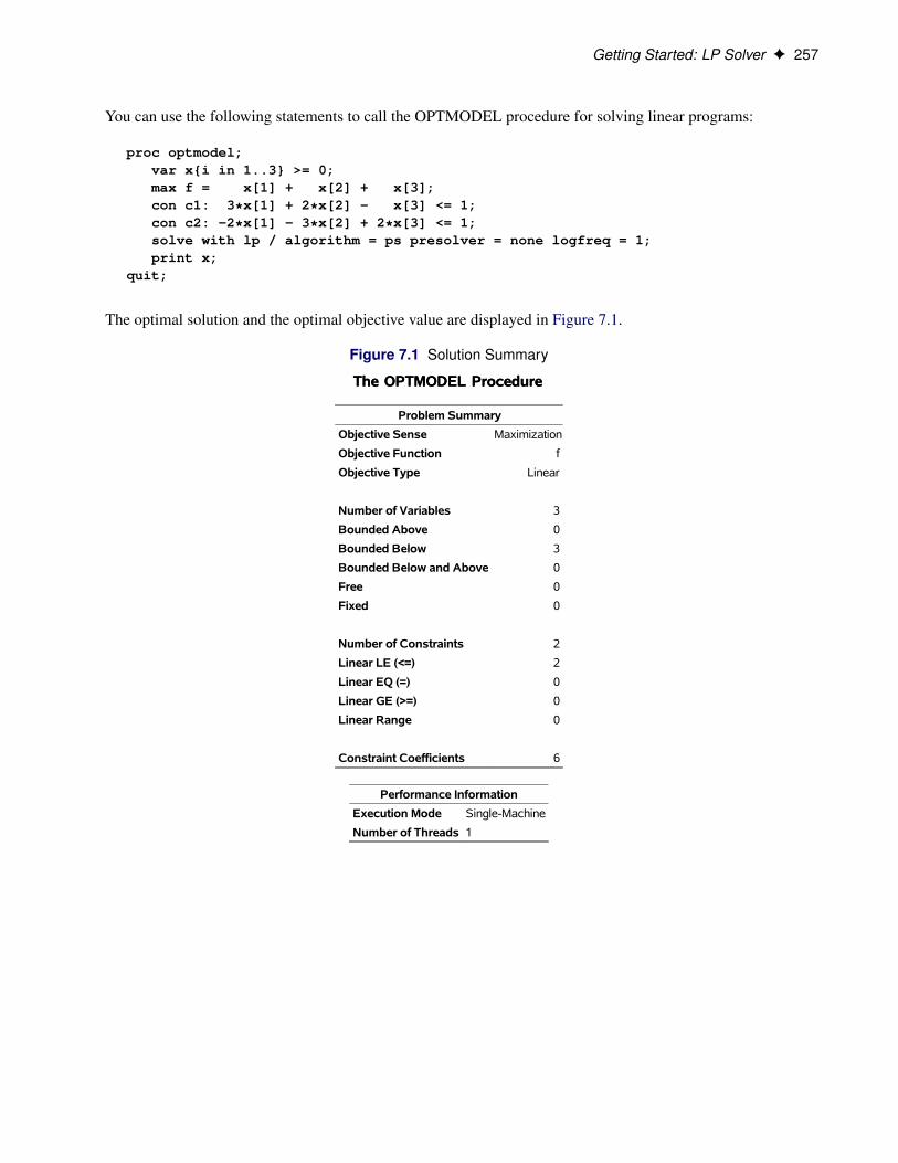
You can use the following statements to call the OPTMODEL procedure for solving linear programs:
proc optmodel;var x{i in 1..3} >= 0;max f = x[1] + x[2] + x[3];con c1: 3*x[1] + 2*x[2] - x[3] <= 1;con c2: -2*x[1] - 3*x[2] + 2*x[3] <= 1;solve with lp / algorithm = ps presolver = none logfreq = 1;print x;
quit;
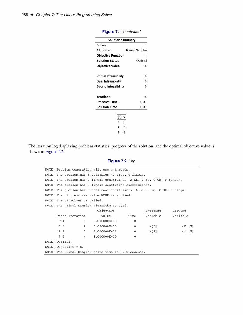
The optimal solution and the optimal objective value are displayed in Figure 7.1.
Figure 7.1 Solution Summary
The OPTMODEL ProcedureThe OPTMODEL Procedure
Problem Summary
Objective Sense Maximization
Objective Function f
Objective Type Linear
Number of Variables 3
Bounded Above 0
Bounded Below 3
Bounded Below and Above 0
Free 0
Fixed 0
Number of Constraints 2
Linear LE (<=) 2
Linear EQ (=) 0
Linear GE (>=) 0
Linear Range 0
Constraint Coefficients 6
Performance Information
Execution Mode Single-Machine
Number of Threads 1
258 F Chapter 7: The Linear Programming Solver
Figure 7.1 continued
Solution Summary
Solver LP
Algorithm Primal Simplex
Objective Function f
Solution Status Optimal
Objective Value 8
Primal Infeasibility 0
Dual Infeasibility 0
Bound Infeasibility 0
Iterations 4
Presolve Time 0.00
Solution Time 0.00
[1] x
1 0
2 3
3 5
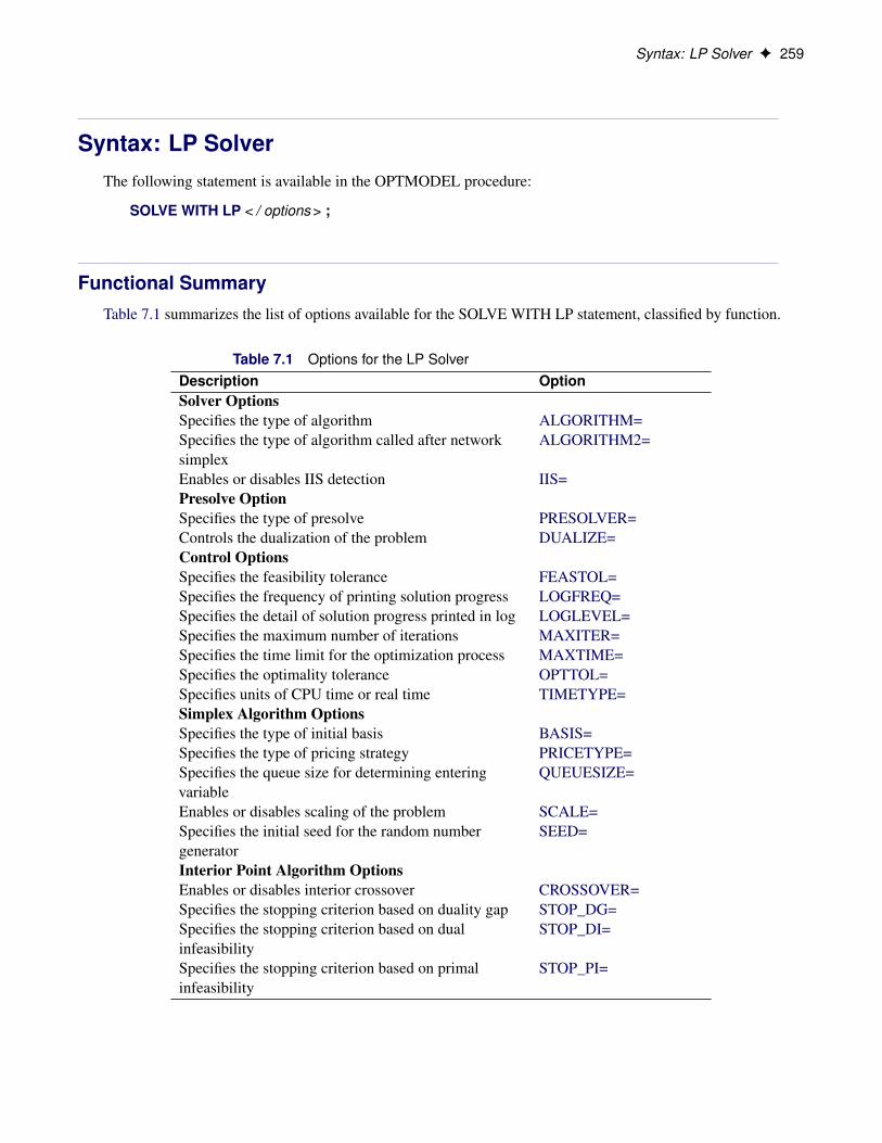
The iteration log displaying problem statistics, progress of the solution, and the optimal objective value isshown in Figure 7.2.
Figure 7.2 Log
NOTE: Problem generation will use 4 threads.
NOTE: The problem has 3 variables (0 free, 0 fixed).
NOTE: The problem has 2 linear constraints (2 LE, 0 EQ, 0 GE, 0 range).
NOTE: The problem has 6 linear constraint coefficients.
NOTE: The problem has 0 nonlinear constraints (0 LE, 0 EQ, 0 GE, 0 range).
NOTE: The LP presolver value NONE is applied.
NOTE: The LP solver is called.
NOTE: The Primal Simplex algorithm is used.
Objective Entering Leaving
Phase Iteration Value Time Variable Variable
P 1 1 0.000000E+00 0
P 2 2 0.000000E+00 0 x[3] c2 (S)
P 2 3 5.000000E-01 0 x[2] c1 (S)
P 2 4 8.000000E+00 0
NOTE: Optimal.
NOTE: Objective = 8.
NOTE: The Primal Simplex solve time is 0.00 seconds.
Syntax: LP Solver F 259
Syntax: LP SolverThe following statement is available in the OPTMODEL procedure:
SOLVE WITH LP < / options > ;
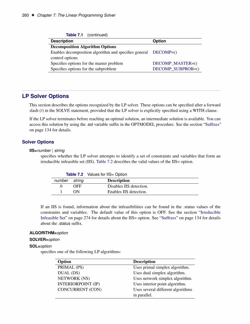
Functional SummaryTable 7.1 summarizes the list of options available for the SOLVE WITH LP statement, classified by function.
Table 7.1 Options for the LP SolverDescription OptionSolver OptionsSpecifies the type of algorithm ALGORITHM=Specifies the type of algorithm called after networksimplex
ALGORITHM2=
Enables or disables IIS detection IIS=Presolve OptionSpecifies the type of presolve PRESOLVER=Controls the dualization of the problem DUALIZE=Control OptionsSpecifies the feasibility tolerance FEASTOL=Specifies the frequency of printing solution progress LOGFREQ=Specifies the detail of solution progress printed in log LOGLEVEL=Specifies the maximum number of iterations MAXITER=Specifies the time limit for the optimization process MAXTIME=Specifies the optimality tolerance OPTTOL=Specifies units of CPU time or real time TIMETYPE=Simplex Algorithm OptionsSpecifies the type of initial basis BASIS=Specifies the type of pricing strategy PRICETYPE=Specifies the queue size for determining enteringvariable
QUEUESIZE=
Enables or disables scaling of the problem SCALE=Specifies the initial seed for the random numbergenerator
SEED=
Interior Point Algorithm OptionsEnables or disables interior crossover CROSSOVER=Specifies the stopping criterion based on duality gap STOP_DG=Specifies the stopping criterion based on dualinfeasibility
STOP_DI=
Specifies the stopping criterion based on primalinfeasibility
STOP_PI=
260 F Chapter 7: The Linear Programming Solver
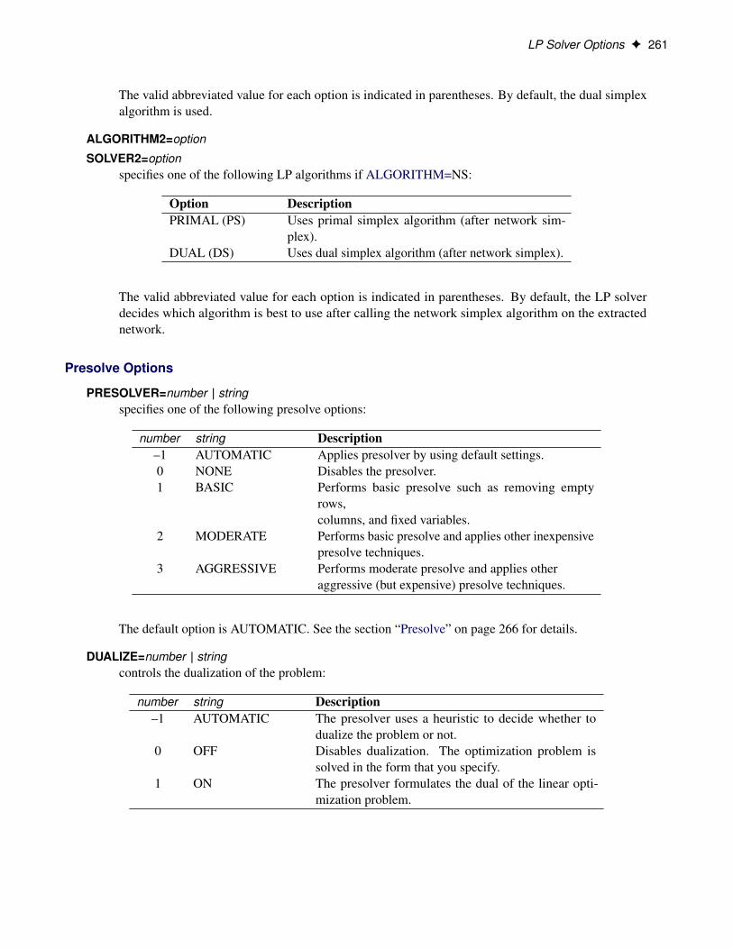
Table 7.1 (continued)Description OptionDecomposition Algorithm OptionsEnables decomposition algorithm and specifies generalcontrol options
DECOMP=()
Specifies options for the master problem DECOMP_MASTER=()Specifies options for the subproblem DECOMP_SUBPROB=()
LP Solver OptionsThis section describes the options recognized by the LP solver. These options can be specified after a forwardslash (/) in the SOLVE statement, provided that the LP solver is explicitly specified using a WITH clause.
If the LP solver terminates before reaching an optimal solution, an intermediate solution is available. You canaccess this solution by using the .sol variable suffix in the OPTMODEL procedure. See the section “Suffixes”on page 134 for details.
Solver Options
IIS=number j stringspecifies whether the LP solver attempts to identify a set of constraints and variables that form anirreducible infeasible set (IIS). Table 7.2 describes the valid values of the IIS= option.
Table 7.2 Values for IIS= Optionnumber string Description
0 OFF Disables IIS detection.1 ON Enables IIS detection.
If an IIS is found, information about the infeasibilities can be found in the .status values of theconstraints and variables. The default value of this option is OFF. See the section “IrreducibleInfeasible Set” on page 274 for details about the IIS= option. See “Suffixes” on page 134 for detailsabout the .status suffix.
ALGORITHM=option
SOLVER=option
SOL=optionspecifies one of the following LP algorithms:
Option DescriptionPRIMAL (PS) Uses primal simplex algorithm.DUAL (DS) Uses dual simplex algorithm.NETWORK (NS) Uses network simplex algorithm.INTERIORPOINT (IP) Uses interior point algorithm.CONCURRENT (CON) Uses several different algorithms
in parallel.
LP Solver Options F 261
The valid abbreviated value for each option is indicated in parentheses. By default, the dual simplexalgorithm is used.
ALGORITHM2=option
SOLVER2=optionspecifies one of the following LP algorithms if ALGORITHM=NS:
Option DescriptionPRIMAL (PS) Uses primal simplex algorithm (after network sim-
plex).DUAL (DS) Uses dual simplex algorithm (after network simplex).
The valid abbreviated value for each option is indicated in parentheses. By default, the LP solverdecides which algorithm is best to use after calling the network simplex algorithm on the extractednetwork.
Presolve Options
PRESOLVER=number | stringspecifies one of the following presolve options:
number string Description–1 AUTOMATIC Applies presolver by using default settings.0 NONE Disables the presolver.1 BASIC Performs basic presolve such as removing empty
rows,columns, and fixed variables.
2 MODERATE Performs basic presolve and applies other inexpensivepresolve techniques.
3 AGGRESSIVE Performs moderate presolve and applies otheraggressive (but expensive) presolve techniques.
The default option is AUTOMATIC. See the section “Presolve” on page 266 for details.
DUALIZE=number | stringcontrols the dualization of the problem:
number string Description–1 AUTOMATIC The presolver uses a heuristic to decide whether to
dualize the problem or not.0 OFF Disables dualization. The optimization problem is
solved in the form that you specify.1 ON The presolver formulates the dual of the linear opti-
mization problem.
262 F Chapter 7: The Linear Programming Solver
Dualization is usually helpful for problems that have many more constraints than variables. You canuse this option with all simplex algorithms in the SOLVE WITH LP statement, but it is most effectivewith the primal and dual simplex algorithms.
The default option is AUTOMATIC.
Control Options
FEASTOL=�specifies the feasibility tolerance, � 2[1E–9, 1E–4], for determining the feasibility of a variable. Thedefault value is 1E–6.
LOGFREQ=k
PRINTFREQ=kspecifies that the printing of the solution progress to the iteration log is to occur after every k iterations.The print frequency, k , is an integer between zero and the largest four-byte signed integer, which is231 � 1.
The value k = 0 disables the printing of the progress of the solution. If the primal or dual simplexalgorithms are used, the default value of this option is determined dynamically according to the problemsize. If the network simplex algorithm is used, the default value of this option is 10,000. If the interiorpoint algorithm is used, the default value of this option is 1.
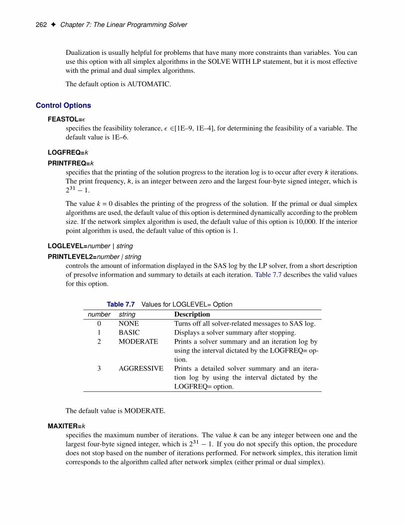
LOGLEVEL=number | string
PRINTLEVEL2=number | stringcontrols the amount of information displayed in the SAS log by the LP solver, from a short descriptionof presolve information and summary to details at each iteration. Table 7.7 describes the valid valuesfor this option.
Table 7.7 Values for LOGLEVEL= Optionnumber string Description
0 NONE Turns off all solver-related messages to SAS log.1 BASIC Displays a solver summary after stopping.2 MODERATE Prints a solver summary and an iteration log by
using the interval dictated by the LOGFREQ= op-tion.
3 AGGRESSIVE Prints a detailed solver summary and an itera-tion log by using the interval dictated by theLOGFREQ= option.
The default value is MODERATE.
MAXITER=kspecifies the maximum number of iterations. The value k can be any integer between one and thelargest four-byte signed integer, which is 231 � 1. If you do not specify this option, the proceduredoes not stop based on the number of iterations performed. For network simplex, this iteration limitcorresponds to the algorithm called after network simplex (either primal or dual simplex).
LP Solver Options F 263
MAXTIME=tspecifies an upper limit of t units of time for the optimization process, including problem generationtime and solution time. The value of the TIMETYPE= option determines the type of units used. If youdo not specify the MAXTIME= option, the solver does not stop based on the amount of time elapsed.The value of t can be any positive number; the default value is the positive number that has the largestabsolute value that can be represented in your operating environment.
OPTTOL=�specifies the optimality tolerance, � 2 [1E–9, 1E–4], for declaring optimality. The default value is1E–6.
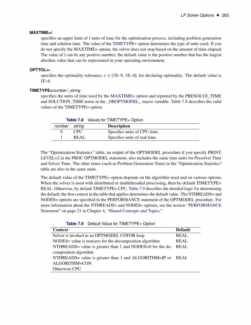
TIMETYPE=number j stringspecifies the units of time used by the MAXTIME= option and reported by the PRESOLVE_TIMEand SOLUTION_TIME terms in the _OROPTMODEL_ macro variable. Table 7.8 describes the validvalues of the TIMETYPE= option.
Table 7.8 Values for TIMETYPE= Optionnumber string Description
0 CPU Specifies units of CPU time.1 REAL Specifies units of real time.
The “Optimization Statistics” table, an output of the OPTMODEL procedure if you specify PRINT-LEVEL=2 in the PROC OPTMODEL statement, also includes the same time units for Presolver Timeand Solver Time. The other times (such as Problem Generation Time) in the “Optimization Statistics”table are also in the same units.
The default value of the TIMETYPE= option depends on the algorithm used and on various options.When the solver is used with distributed or multithreaded processing, then by default TIMETYPE=REAL. Otherwise, by default TIMETYPE= CPU. Table 7.9 describes the detailed logic for determiningthe default; the first context in the table that applies determines the default value. The NTHREADS= andNODES= options are specified in the PERFORMANCE statement of the OPTMODEL procedure. Formore information about the NTHREADS= and NODES= options, see the section “PERFORMANCEStatement” on page 21 in Chapter 4, “Shared Concepts and Topics.”
Table 7.9 Default Value for TIMETYPE= OptionContext DefaultSolver is invoked in an OPTMODEL COFOR loop REALNODES= value is nonzero for the decomposition algorithm REALNTHREADS= value is greater than 1 and NODES=0 for the de-composition algorithm
REAL
NTHREADS= value is greater than 1 and ALGORITHM=IP orALGORITHM=CON
REAL
Otherwise CPU
264 F Chapter 7: The Linear Programming Solver
Simplex Algorithm Options
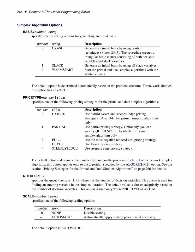
BASIS=number | stringspecifies the following options for generating an initial basis:
number string Description0 CRASH Generate an initial basis by using crash
techniques (Maros 2003). The procedure creates atriangular basic matrix consisting of both decisionvariables and slack variables.
1 SLACK Generate an initial basis by using all slack variables.2 WARMSTART Start the primal and dual simplex algorithms with the
available basis.
The default option is determined automatically based on the problem structure. For network simplex,this option has no effect.
PRICETYPE=number | stringspecifies one of the following pricing strategies for the primal and dual simplex algorithms:
number string Description0 HYBRID Use hybrid Devex and steepest-edge pricing
strategies. Available for primal simplex algorithmonly.
1 PARTIAL Use partial pricing strategy. Optionally, you canspecify QUEUESIZE=. Available for primalsimplex algorithm only.
2 FULL Use the most negative reduced cost pricing strategy.3 DEVEX Use Devex pricing strategy.4 STEEPESTEDGE Use steepest-edge pricing strategy.
The default option is determined automatically based on the problem structure. For the network simplexalgorithm, this option applies only to the algorithm specified by the ALGORITHM2= option. See thesection “Pricing Strategies for the Primal and Dual Simplex Algorithms” on page 266 for details.
QUEUESIZE=kspecifies the queue size, k 2 Œ1; n�, where n is the number of decision variables. This queue is used forfinding an entering variable in the simplex iteration. The default value is chosen adaptively based onthe number of decision variables. This option is used only when PRICETYPE=PARTIAL.
SCALE=number | stringspecifies one of the following scaling options:
number string Description0 NONE Disable scaling.–1 AUTOMATIC Automatically apply scaling procedure if necessary.
The default option is AUTOMATIC.
LP Solver Options F 265
SEED=numberspecifies the initial seed for the random number generator. Because the seed affects the perturbationin the simplex algorithms, the result might be a different optimal solution and a different solver path,but the effect is usually negligible. The value of number can be any positive integer up to the largestfour-byte signed integer, which is 231 � 1. By default, SEED=100.
Interior Point Algorithm Options
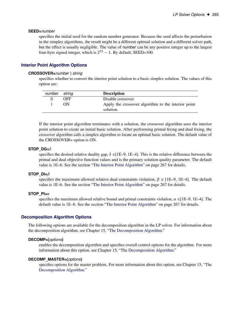
CROSSOVER=number | stringspecifies whether to convert the interior point solution to a basic simplex solution. The values of thisoption are:
number string Description0 OFF Disable crossover.1 ON Apply the crossover algorithm to the interior point
solution.
If the interior point algorithm terminates with a solution, the crossover algorithm uses the interiorpoint solution to create an initial basic solution. After performing primal fixing and dual fixing, thecrossover algorithm calls a simplex algorithm to locate an optimal basic solution. The default value ofthe CROSSOVER= option is ON.
STOP_DG=ıspecifies the desired relative duality gap, ı 2[1E–9, 1E–4]. This is the relative difference between theprimal and dual objective function values and is the primary solution quality parameter. The defaultvalue is 1E–6. See the section “The Interior Point Algorithm” on page 267 for details.
STOP_DI=ˇspecifies the maximum allowed relative dual constraints violation, ˇ 2 [1E–9, 1E–4]. The defaultvalue is 1E–6. See the section “The Interior Point Algorithm” on page 267 for details.
STOP_PI=˛specifies the maximum allowed relative bound and primal constraints violation, ˛ 2[1E–9, 1E–4]. Thedefault value is 1E–6. See the section “The Interior Point Algorithm” on page 267 for details.
Decomposition Algorithm Options
The following options are available for the decomposition algorithm in the LP solver. For information aboutthe decomposition algorithm, see Chapter 15, “The Decomposition Algorithm.”
DECOMP=(options)enables the decomposition algorithm and specifies overall control options for the algorithm. For moreinformation about this option, see Chapter 15, “The Decomposition Algorithm.”
DECOMP_MASTER=(options)specifies options for the master problem. For more information about this option, see Chapter 15, “TheDecomposition Algorithm.”
266 F Chapter 7: The Linear Programming Solver
DECOMP_SUBPROB=(options)specifies option for the subproblem. For more information about this option, see Chapter 15, “TheDecomposition Algorithm.”
Details: LP Solver
PresolvePresolve in the simplex LP algorithms of PROC OPTMODEL uses a variety of techniques to reduce theproblem size, improve numerical stability, and detect infeasibility or unboundedness (Andersen and Andersen1995; Gondzio 1997). During presolve, redundant constraints and variables are identified and removed.Presolve can further reduce the problem size by substituting variables. Variable substitution is a very effectivetechnique, but it might occasionally increase the number of nonzero entries in the constraint matrix.
In most cases, using presolve is very helpful in reducing solution times. You can enable presolve at differentlevels or disable it by specifying the PRESOLVER= option.
Pricing Strategies for the Primal and Dual Simplex AlgorithmsSeveral pricing strategies for the primal and dual simplex algorithms are available. Pricing strategiesdetermine which variable enters the basis at each simplex pivot. These can be controlled by specifying thePRICETYPE= option.
The primal simplex algorithm has the following five pricing strategies:
PARTIAL scans a queue of decision variables to find an entering variable. You can optionallyspecify the QUEUESIZE= option to control the length of this queue.
FULL uses Dantzig’s most violated reduced cost rule (Dantzig 1963). It compares thereduced cost of all decision variables, and selects the variable with the most violatedreduced cost as the entering variable.
DEVEX implements the Devex pricing strategy developed by Harris (1973).
STEEPESTEDGE uses the steepest-edge pricing strategy developed by Forrest and Goldfarb (1992).
HYBRID uses a hybrid of the Devex and steepest-edge pricing strategies.
The dual simplex algorithm has only three pricing strategies available: FULL, DEVEX, and STEEPEST-EDGE.
The Network Simplex AlgorithmThe network simplex algorithm in PROC OPTMODEL attempts to leverage the speed of the network simplexalgorithm to more efficiently solve linear programs by using the following process:
The Interior Point Algorithm F 267
1. It heuristically extracts the largest possible network substructure from the original problem.
2. It uses the network simplex algorithm to solve for an optimal solution to this substructure.
3. It uses this solution to construct an advanced basis to warm-start either the primal or dual simplexalgorithm on the original linear programming problem.
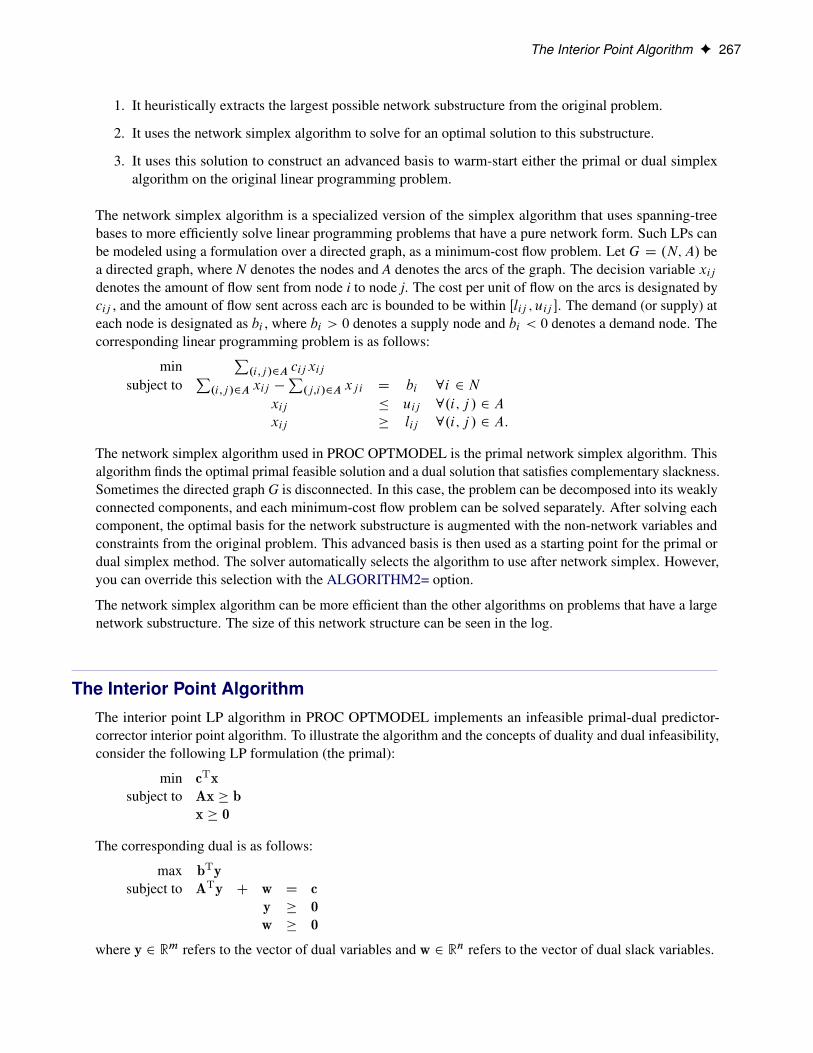
The network simplex algorithm is a specialized version of the simplex algorithm that uses spanning-treebases to more efficiently solve linear programming problems that have a pure network form. Such LPs canbe modeled using a formulation over a directed graph, as a minimum-cost flow problem. Let G D .N;A/ bea directed graph, where N denotes the nodes and A denotes the arcs of the graph. The decision variable xij
denotes the amount of flow sent from node i to node j. The cost per unit of flow on the arcs is designated bycij , and the amount of flow sent across each arc is bounded to be within Œlij ; uij �. The demand (or supply) ateach node is designated as bi , where bi > 0 denotes a supply node and bi < 0 denotes a demand node. Thecorresponding linear programming problem is as follows:
minP
.i;j /2A cijxij
subject toP
.i;j /2A xij �P
.j;i/2A xj i D bi 8i 2 N
xij � uij 8.i; j / 2 A
xij � lij 8.i; j / 2 A:
The network simplex algorithm used in PROC OPTMODEL is the primal network simplex algorithm. Thisalgorithm finds the optimal primal feasible solution and a dual solution that satisfies complementary slackness.Sometimes the directed graph G is disconnected. In this case, the problem can be decomposed into its weaklyconnected components, and each minimum-cost flow problem can be solved separately. After solving eachcomponent, the optimal basis for the network substructure is augmented with the non-network variables andconstraints from the original problem. This advanced basis is then used as a starting point for the primal ordual simplex method. The solver automatically selects the algorithm to use after network simplex. However,you can override this selection with the ALGORITHM2= option.
The network simplex algorithm can be more efficient than the other algorithms on problems that have a largenetwork substructure. The size of this network structure can be seen in the log.
The Interior Point AlgorithmThe interior point LP algorithm in PROC OPTMODEL implements an infeasible primal-dual predictor-corrector interior point algorithm. To illustrate the algorithm and the concepts of duality and dual infeasibility,consider the following LP formulation (the primal):
min cTxsubject to Ax � b
x � 0
The corresponding dual is as follows:
max bTysubject to ATy C w D c
y � 0w � 0
where y 2 Rm refers to the vector of dual variables and w 2 Rn refers to the vector of dual slack variables.
268 F Chapter 7: The Linear Programming Solver
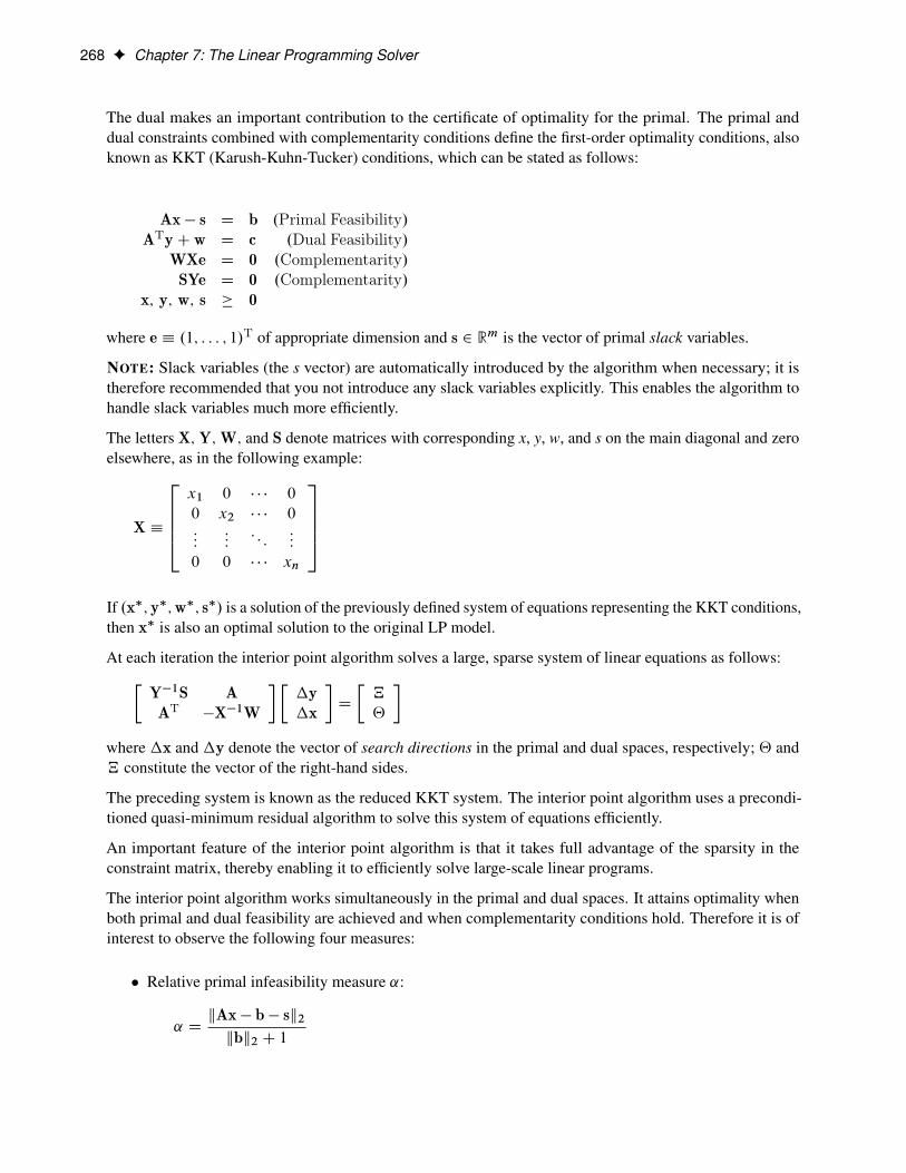
The dual makes an important contribution to the certificate of optimality for the primal. The primal anddual constraints combined with complementarity conditions define the first-order optimality conditions, alsoknown as KKT (Karush-Kuhn-Tucker) conditions, which can be stated as follows:
Ax � s D b .Primal Feasibility/ATyC w D c .Dual Feasibility/
WXe D 0 .Complementarity/SYe D 0 .Complementarity/
x; y; w; s � 0
where e � .1; : : : ; 1/T of appropriate dimension and s 2 Rm is the vector of primal slack variables.
NOTE: Slack variables (the s vector) are automatically introduced by the algorithm when necessary; it istherefore recommended that you not introduce any slack variables explicitly. This enables the algorithm tohandle slack variables much more efficiently.
The letters X; Y;W; and S denote matrices with corresponding x, y, w, and s on the main diagonal and zeroelsewhere, as in the following example:
X �
26664x1 0 � � � 0
0 x2 � � � 0:::
:::: : :
:::
0 0 � � � xn
37775If .x�; y�;w�; s�/ is a solution of the previously defined system of equations representing the KKT conditions,then x� is also an optimal solution to the original LP model.
At each iteration the interior point algorithm solves a large, sparse system of linear equations as follows:�Y�1S AAT �X�1W
� ��y�x
�D
�„
‚
�where �x and �y denote the vector of search directions in the primal and dual spaces, respectively; ‚ and„ constitute the vector of the right-hand sides.
The preceding system is known as the reduced KKT system. The interior point algorithm uses a precondi-tioned quasi-minimum residual algorithm to solve this system of equations efficiently.
An important feature of the interior point algorithm is that it takes full advantage of the sparsity in theconstraint matrix, thereby enabling it to efficiently solve large-scale linear programs.
The interior point algorithm works simultaneously in the primal and dual spaces. It attains optimality whenboth primal and dual feasibility are achieved and when complementarity conditions hold. Therefore it is ofinterest to observe the following four measures:
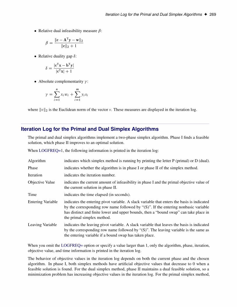
� Relative primal infeasibility measure ˛:
˛ DkAx � b � sk2kbk2 C 1
Iteration Log for the Primal and Dual Simplex Algorithms F 269
� Relative dual infeasibility measure ˇ:
ˇ Dkc �ATy � wk2kck2 C 1
� Relative duality gap ı:
ı DjcTx � bTyjjcTxj C 1
� Absolute complementarity :
D
nXiD1
xiwi C
mXiD1
yisi
where kvk2 is the Euclidean norm of the vector v. These measures are displayed in the iteration log.
Iteration Log for the Primal and Dual Simplex AlgorithmsThe primal and dual simplex algorithms implement a two-phase simplex algorithm. Phase I finds a feasiblesolution, which phase II improves to an optimal solution.
When LOGFREQ=1, the following information is printed in the iteration log:
Algorithm indicates which simplex method is running by printing the letter P (primal) or D (dual).
Phase indicates whether the algorithm is in phase I or phase II of the simplex method.
Iteration indicates the iteration number.
Objective Value indicates the current amount of infeasibility in phase I and the primal objective value ofthe current solution in phase II.
Time indicates the time elapsed (in seconds).
Entering Variable indicates the entering pivot variable. A slack variable that enters the basis is indicatedby the corresponding row name followed by “(S)”. If the entering nonbasic variablehas distinct and finite lower and upper bounds, then a “bound swap” can take place inthe primal simplex method.
Leaving Variable indicates the leaving pivot variable. A slack variable that leaves the basis is indicatedby the corresponding row name followed by “(S)”. The leaving variable is the same asthe entering variable if a bound swap has taken place.
When you omit the LOGFREQ= option or specify a value larger than 1, only the algorithm, phase, iteration,objective value, and time information is printed in the iteration log.
The behavior of objective values in the iteration log depends on both the current phase and the chosenalgorithm. In phase I, both simplex methods have artificial objective values that decrease to 0 when afeasible solution is found. For the dual simplex method, phase II maintains a dual feasible solution, so aminimization problem has increasing objective values in the iteration log. For the primal simplex method,
270 F Chapter 7: The Linear Programming Solver
phase II maintains a primal feasible solution, so a minimization problem has decreasing objective values inthe iteration log.
During the solution process, some elements of the LP model might be perturbed to improve performance. Inthis case the objective values that are printed correspond to the perturbed problem. After reaching optimalityfor the perturbed problem, the LP solver solves the original problem by switching from the primal simplexmethod to the dual simplex method (or from the dual simplex method to the primal simplex method). Becausethe problem might be perturbed again, this process can result in several changes between the two algorithms.
Iteration Log for the Network Simplex AlgorithmAfter finding the embedded network and formulating the appropriate relaxation, the network simplexalgorithm uses a primal network simplex algorithm. In the case of a connected network, with one (weaklyconnected) component, the log will show the progress of the simplex algorithm. The following informationis displayed in the iteration log:
Iteration indicates the iteration number.
PrimalObj indicates the primal objective value of the current solution.
Primal Infeas indicates the maximum primal infeasibility of the current solution.
Time indicates the time spent on the current component by network simplex.
The frequency of the simplex iteration log is controlled by the LOGFREQ= option. The default value of theLOGFREQ= option is 10,000.
If the network relaxation is disconnected, the information in the iteration log shows progress at the componentlevel. The following information is displayed in the iteration log:
Component indicates the component number being processed.
Nodes indicates the number of nodes in this component.
Arcs indicates the number of arcs in this component.
Iterations indicates the number of simplex iterations needed to solve this component.
Time indicates the time spent so far in network simplex.
The frequency of the component iteration log is controlled by the LOGFREQ= option. In this case, thedefault value of the LOGFREQ= option is determined by the size of the network.
The LOGLEVEL= option adjusts the amount of detail shown. By default, LOGLEVEL=MODERATEand reports as in the preceding description. If LOGLEVEL=NONE, no information is shown. IfLOGLEVEL=BASIC, the only information shown is a summary of the network relaxation and the time spentsolving the relaxation. If LOGLEVEL=AGGRESSIVE, in the case of one component, the log displays asin the preceding description; in the case of multiple components, for each component, a separate simplexiteration log is displayed.
Iteration Log for the Interior Point Algorithm F 271
Iteration Log for the Interior Point AlgorithmThe interior point algorithm implements an infeasible primal-dual predictor-corrector interior point algorithm.The following information is displayed in the iteration log:
Iter indicates the iteration number
Complement indicates the (absolute) complementarity
Duality Gap indicates the (relative) duality gap
Primal Infeas indicates the (relative) primal infeasibility measure
Bound Infeas indicates the (relative) bound infeasibility measure
Dual Infeas indicates the (relative) dual infeasibility measure
Time indicates the time elapsed (in seconds).
If the sequence of solutions converges to an optimal solution of the problem, you should see all columnsin the iteration log converge to zero or very close to zero. If they do not, it can be the result of insufficientiterations being performed to reach optimality. In this case, you might need to increase the value specified inthe option MAXITER= or MAXTIME=. If the complementarity and/or the duality gap do not converge, theproblem might be infeasible or unbounded. If the infeasibility columns do not converge, the problem mightbe infeasible.
Iteration Log for the Crossover AlgorithmThe crossover algorithm takes an optimal solution from the interior point algorithm and transforms it intoan optimal basic solution. The iterations of the crossover algorithm are similar to simplex iterations; thissimilarity is reflected in the format of the iteration logs.
When LOGFREQ=1, the following information is printed in the iteration log:
Phase indicates whether the primal crossover (PC) or dual crossover (DC) technique is used.
Iteration indicates the iteration number.
Objective Value indicates the total amount by which the superbasic variables are off their bound. Thisvalue decreases to 0 as the crossover algorithm progresses.
Time indicates the time elapsed (in seconds).
Entering Variable indicates the entering pivot variable. A slack variable that enters the basis is indicatedby the corresponding row name followed by “(S)”.
Leaving Variable indicates the leaving pivot variable. A slack variable that leaves the basis is indicated bythe corresponding row name followed by “(S)”.
When you omit the LOGFREQ= option or specify a value greater than 1, only the phase, iteration, objectivevalue, and time information are printed in the iteration log.
After all the superbasic variables have been eliminated, the crossover algorithm continues with regular primalor dual simplex iterations.
272 F Chapter 7: The Linear Programming Solver
Concurrent LPThe ALGORITHM=CON option starts several different linear optimization algorithms in parallel in asingle-machine mode. The LP solver automatically determines which algorithms to run and how manythreads to assign to each algorithm. If sufficient resources are available, the solver runs all four standardalgorithms. When the first algorithm finishes, the LP solver returns the results from that algorithm andterminates any other algorithms that are still running. If you specify a value of DETERMINISTIC forthe PARALLELMODE= option in the PERFORMANCE statement in the OPTMODEL procedure, thealgorithm for which the results are returned is not necessarily the one that finished first. The LP solverdeterministically selects the algorithm for which the results are returned. For more information about thePERFORMANCE statement, see the section “PERFORMANCE Statement” on page 21. Regardless of whichmode (deterministic or nondeterministic) is in effect, terminating algorithms that are still running might takea significant amount of time.
During concurrent optimization, the procedure displays the iteration log for the dual simplex algorithm. Seethe section “Iteration Log for the Primal and Dual Simplex Algorithms” on page 269 for more informationabout this iteration log. Upon termination, the solver displays the iteration log for the algorithm that finishesfirst, unless the dual simplex algorithm finishes first. If you specify LOGLEVEL=AGGRESSIVE, the LPsolver displays the iteration logs for all algorithms that were run concurrently.
If you specify PRINTLEVEL=2 in the PROC OPTMODEL statement and ALGORITHM=CON in theSOLVE WITH LP statement, the LP solver produces an ODS table called ConcurrentSummary. This tablecontains a summary of the solution statuses of all algorithms that are run concurrently.
Parallel ProcessingThe interior point and concurrent LP algorithms can be run in single-machine mode (in single-machine mode,the computation is executed by multiple threads on a single computer). The decomposition algorithm canbe run in either single-machine or distributed mode (in distributed mode, the computation is executed onmultiple computing nodes in a distributed computing environment).
NOTE: Distributed mode requires SAS High-Performance Optimization.
You can specify options for parallel processing in the PERFORMANCE statement, which is documented inthe section “PERFORMANCE Statement” on page 21 in Chapter 4, “Shared Concepts and Topics.”
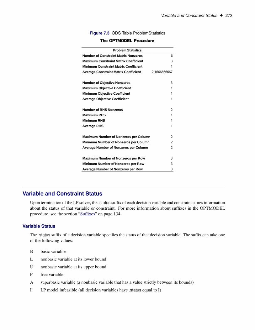
Problem StatisticsOptimizers can encounter difficulty when solving poorly formulated models. Information about datamagnitude provides a simple gauge to determine how well a model is formulated. For example, a modelwhose constraint matrix contains one very large entry (on the order of 109) can cause difficulty when theremaining entries are single-digit numbers. The PRINTLEVEL=2 option in the OPTMODEL procedurecauses the ODS table “ProblemStatistics” to be generated when the LP solver is called. This table providesbasic data magnitude information that enables you to improve the formulation of your models.
The example output in Figure 7.3 demonstrates the contents of the ODS table “ProblemStatistics.”
Variable and Constraint Status F 273
Figure 7.3 ODS Table ProblemStatistics
The OPTMODEL ProcedureThe OPTMODEL Procedure
Problem Statistics
Number of Constraint Matrix Nonzeros 6
Maximum Constraint Matrix Coefficient 3
Minimum Constraint Matrix Coefficient 1
Average Constraint Matrix Coefficient 2.1666666667
Number of Objective Nonzeros 3
Maximum Objective Coefficient 1
Minimum Objective Coefficient 1
Average Objective Coefficient 1
Number of RHS Nonzeros 2
Maximum RHS 1
Minimum RHS 1
Average RHS 1
Maximum Number of Nonzeros per Column 2
Minimum Number of Nonzeros per Column 2
Average Number of Nonzeros per Column 2
Maximum Number of Nonzeros per Row 3
Minimum Number of Nonzeros per Row 3
Average Number of Nonzeros per Row 3
Variable and Constraint StatusUpon termination of the LP solver, the .status suffix of each decision variable and constraint stores informationabout the status of that variable or constraint. For more information about suffixes in the OPTMODELprocedure, see the section “Suffixes” on page 134.
Variable Status
The .status suffix of a decision variable specifies the status of that decision variable. The suffix can take oneof the following values:
B basic variable
L nonbasic variable at its lower bound
U nonbasic variable at its upper bound
F free variable
A superbasic variable (a nonbasic variable that has a value strictly between its bounds)
I LP model infeasible (all decision variables have .status equal to I)
274 F Chapter 7: The Linear Programming Solver
For the interior point algorithm with IIS= OFF, .status is blank.
The following values can appear only if IIS= ON. See the section “Irreducible Infeasible Set” on page 274for details.
I_L the lower bound of the variable is needed for the IIS
I_U the upper bound of the variable is needed for the IIS
I_F both bounds of the variable are needed for the IIS (the variable is fixed or has conflicting bounds)
Constraint Status
The .status suffix of a constraint specifies the status of the slack variable for that constraint. The suffix cantake one of the following values:
B basic variable
L nonbasic variable at its lower bound
U nonbasic variable at its upper bound
F free variable
A superbasic variable (a nonbasic variable that has a value strictly between its bounds)
I LP model infeasible (all decision variables have .status equal to I)
The following values can appear only if option IIS= ON. See the section “Irreducible Infeasible Set” onpage 274 for details.
I_L the “GE” (�) condition of the constraint is needed for the IIS
I_U the “LE” (�) condition of the constraint is needed for the IIS
I_F both conditions of the constraint are needed for the IIS (the constraint is an equality or a range constraintwith conflicting bounds)
Irreducible Infeasible SetFor a linear programming problem, an irreducible infeasible set (IIS) is an infeasible subset of constraints andvariable bounds that will become feasible if any single constraint or variable bound is removed. It is possibleto have more than one IIS in an infeasible LP. Identifying an IIS can help isolate the structural infeasibility inan LP.
The presolver in the LP algorithms can detect infeasibility, but it identifies only the variable bound orconstraint that triggers the infeasibility.
The IIS=ON option directs the LP solver to search for an IIS in a specified LP. You should specify theOPTMODEL option PRESOLVER=NONE when you specify IIS=ON; otherwise the IIS results can beincomplete. The LP solver does not apply the LP presolver to the problem during the IIS search. If the LPsolver detects an IIS, it updates the .status suffix of the decision variables and constraints, and then it stops.The number of iterations that are reported in the macro variable and the ODS table is the total number of
Macro Variable _OROPTMODEL_ F 275
simplex iterations. This total includes the initial LP solve and all subsequent iterations during the constraintdeletion phase.
The IIS= option can add special values to the .status suffixes of variables and constraints. (For moreinformation, see the section “Variable and Constraint Status” on page 273.) For constraints, a status of “I_L”,“I_U”, or “I_F” indicates that the “GE” (�), “LE” (�), or “EQ” (=) constraint, respectively, is part of the IIS.For range constraints, a status of “I_L” or “I_U” indicates that the lower or upper bound, respectively, ofthe constraint is needed for the IIS, and “I_F” indicates that the bounds in the constraint are conflicting. Forvariables, a status of “I_L”, “I_U”, or “I_F” indicates that the lower, upper, or both bounds, respectively, ofthe variable are needed for the IIS. From this information, you can identify both the names of the constraints(variables) in the IIS and the corresponding bound where infeasibility occurs.
Making any one of the constraints or variable bounds in the IIS nonbinding removes the infeasibility fromthe IIS. In some cases, changing a right-hand side or bound by a finite amount removes the infeasibility.However, the only way to guarantee removal of the infeasibility is to set the appropriate right-hand side orbound to1 or �1. Because it is possible for an LP to have multiple irreducible infeasible sets, simplyremoving the infeasibility from one set might not make the entire problem feasible. To make the entireproblem feasible, you can specify IIS=ON and rerun the LP solver after removing the infeasibility from anIIS. Repeating this process until the LP solver no longer detects an IIS results in a feasible problem. Thisapproach to infeasibility repair can produce different end problems depending on which right-hand sides andbounds you choose to relax.
The IIS= option in the LP solver uses two different methods to identify an IIS:
1. Based on the result of the initial solve, the sensitivity filter removes several constraints and variablebounds immediately while still maintaining infeasibility. This phase is quick and dramatically reducesthe size of the IIS.
2. Next, the deletion filter removes each remaining constraint and variable bound one by one to checkwhich of them are needed to obtain an infeasible system. This second phase is more time consuming,but it ensures that the IIS set that the LP solver returns is indeed irreducible. The progress of thedeletion filter is reported at regular intervals. The sensitivity filter might be called again during thedeletion filter to improve performance.
See Example 7.4 for an example that demonstrates the use of the IIS= option in locating and removinginfeasibilities.
Macro Variable _OROPTMODEL_The OPTMODEL procedure always creates and initializes a SAS macro called _OROPTMODEL_. Thisvariable contains a character string. After each PROC OROPTMODEL run, you can examine this macro byspecifying %put &_OROPTMODEL_; and check the execution of the most recently invoked solver from thevalue of the macro variable. The various terms of the variable after the LP solver is called are interpreted asfollows.
STATUSindicates the solver status at termination. It can take one of the following values:
276 F Chapter 7: The Linear Programming Solver
OK The solver terminated normally.
SYNTAX_ERROR Incorrect syntax was used.
DATA_ERROR The input data were inconsistent.
OUT_OF_MEMORY Insufficient memory was allocated to the procedure.
IO_ERROR A problem occurred in reading or writing data.
SEMANTIC_ERROR An evaluation error, such as an invalid operand type, occurred.
ERROR The status cannot be classified into any of the preceding categories.
ALGORITHMindicates the algorithm that produces the solution data in the macro variable. This term appears onlywhen STATUS=OK. It can take one of the following values:
PS The primal simplex algorithm produced the solution data.
DS The dual simplex algorithm produced the solution data.
NS The network simplex algorithm produced the solution data.
IP The interior point algorithm produced the solution data.
DECOMP The decomposition algorithm produced the solution data.
When you run algorithms concurrently (ALGORITHM=CON), this term indicates which algorithm isthe first to terminate.
SOLUTION_STATUSindicates the solution status at termination. It can take one of the following values:
OPTIMAL The solution is optimal.
CONDITIONAL_OPTIMAL The solution is optimal, but some infeasibilities (primal,dual or bound) exceed tolerances due to scaling or pre-processing.
FEASIBLE The problem is feasible.
INFEASIBLE The problem is infeasible.
UNBOUNDED The problem is unbounded.
INFEASIBLE_OR_UNBOUNDED The problem is infeasible or unbounded.
BAD_PROBLEM_TYPE The problem type is unsupported by the solver.
ITERATION_LIMIT_REACHED The maximum allowable number of iterations wasreached.
TIME_LIMIT_REACHED The solver reached its execution time limit.
FUNCTION_CALL_LIMIT_REACHED The solver reached its limit on function evaluations.
INTERRUPTED The solver was interrupted externally.
FAILED The solver failed to converge, possibly due to numericalissues.
Macro Variable _OROPTMODEL_ F 277
When SOLUTION_STATUS has a value of OPTIMAL, CONDITIONAL_OPTIMAL, ITERA-TION_LIMIT_REACHED, or TIME_LIMIT_REACHED, all terms of the _OROPTMODEL_ macrovariable are present; for other values of SOLUTION_STATUS, some terms do not appear.
OBJECTIVEindicates the objective value obtained by the solver at termination.
PRIMAL_INFEASIBILITYindicates, for the primal simplex and dual simplex algorithms, the maximum (absolute) violation ofthe primal constraints by the primal solution. For the interior point algorithm, this term indicates therelative violation of the primal constraints by the primal solution.
DUAL_INFEASIBILITYindicates, for the primal simplex and dual simplex algorithms, the maximum (absolute) violation of thedual constraints by the dual solution. For the interior point algorithm, this term indicates the relativeviolation of the dual constraints by the dual solution.
BOUND_INFEASIBILITYindicates, for the primal simplex and dual simplex algorithms, the maximum (absolute) violation of thelower or upper bounds by the primal solution. For the interior point algorithm, this term indicates therelative violation of the lower or upper bounds by the primal solution.
DUALITY_GAPindicates the (relative) duality gap. This term appears only if the option ALGO-RITHM=INTERIORPOINT is specified in the SOLVE statement.
COMPLEMENTARITYindicates the (absolute) complementarity. This term appears only if the option ALGO-RITHM=INTERIORPOINT is specified in the SOLVE statement.
ITERATIONSindicates the number of iterations taken to solve the problem. When the network simplex algorithm isused, this term indicates the number of network simplex iterations taken to solve the network relaxation.When crossover is enabled, this term indicates the number of interior point iterations taken to solve theproblem.
ITERATIONS2indicates the number of simplex iterations performed by the secondary algorithm. The network simplexalgorithm selects the secondary algorithm automatically unless a value has been specified for theALGORITHM2= option. When crossover is enabled, the secondary algorithm is selected automatically.This term appears only if the network simplex algorithm is used or if crossover is enabled.
PRESOLVE_TIMEindicates the time (in seconds) used in preprocessing.
SOLUTION_TIMEindicates the time (in seconds) taken to solve the problem, including preprocessing time.
NOTE: The time reported in PRESOLVE_TIME and SOLUTION_TIME is either CPU time or real time.The type is determined by the TIMETYPE= option.
278 F Chapter 7: The Linear Programming Solver
When SOLUTION_STATUS has a value of OPTIMAL, CONDITIONAL_OPTIMAL, ITERA-TION_LIMIT_REACHED, or TIME_LIMIT_REACHED, all terms of the _OROPTMODEL_ macrovariable are present; for other values of SOLUTION_STATUS, some terms do not appear.
Examples: LP Solver
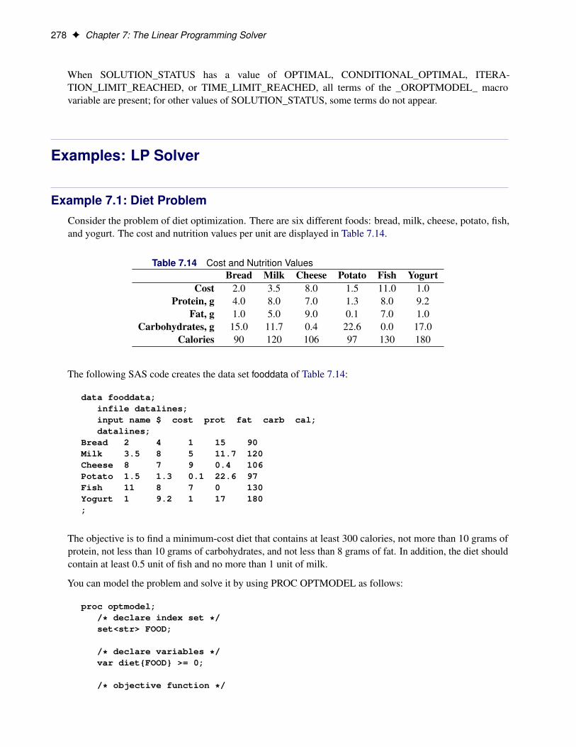
Example 7.1: Diet ProblemConsider the problem of diet optimization. There are six different foods: bread, milk, cheese, potato, fish,and yogurt. The cost and nutrition values per unit are displayed in Table 7.14.
Table 7.14 Cost and Nutrition ValuesBread Milk Cheese Potato Fish Yogurt
Cost 2.0 3.5 8.0 1.5 11.0 1.0Protein, g 4.0 8.0 7.0 1.3 8.0 9.2
Fat, g 1.0 5.0 9.0 0.1 7.0 1.0Carbohydrates, g 15.0 11.7 0.4 22.6 0.0 17.0
Calories 90 120 106 97 130 180
The following SAS code creates the data set fooddata of Table 7.14:
data fooddata;infile datalines;input name $ cost prot fat carb cal;datalines;
Bread 2 4 1 15 90Milk 3.5 8 5 11.7 120Cheese 8 7 9 0.4 106Potato 1.5 1.3 0.1 22.6 97Fish 11 8 7 0 130Yogurt 1 9.2 1 17 180;
The objective is to find a minimum-cost diet that contains at least 300 calories, not more than 10 grams ofprotein, not less than 10 grams of carbohydrates, and not less than 8 grams of fat. In addition, the diet shouldcontain at least 0.5 unit of fish and no more than 1 unit of milk.
You can model the problem and solve it by using PROC OPTMODEL as follows:
proc optmodel;/* declare index set */set<str> FOOD;
/* declare variables */var diet{FOOD} >= 0;
/* objective function */
Example 7.1: Diet Problem F 279
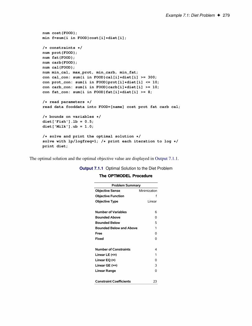
num cost{FOOD};min f=sum{i in FOOD}cost[i]*diet[i];
/* constraints */num prot{FOOD};num fat{FOOD};num carb{FOOD};num cal{FOOD};num min_cal, max_prot, min_carb, min_fat;con cal_con: sum{i in FOOD}cal[i]*diet[i] >= 300;con prot_con: sum{i in FOOD}prot[i]*diet[i] <= 10;con carb_con: sum{i in FOOD}carb[i]*diet[i] >= 10;con fat_con: sum{i in FOOD}fat[i]*diet[i] >= 8;
/* read parameters */read data fooddata into FOOD=[name] cost prot fat carb cal;
/* bounds on variables */diet['Fish'].lb = 0.5;diet['Milk'].ub = 1.0;
/* solve and print the optimal solution */solve with lp/logfreq=1; /* print each iteration to log */print diet;
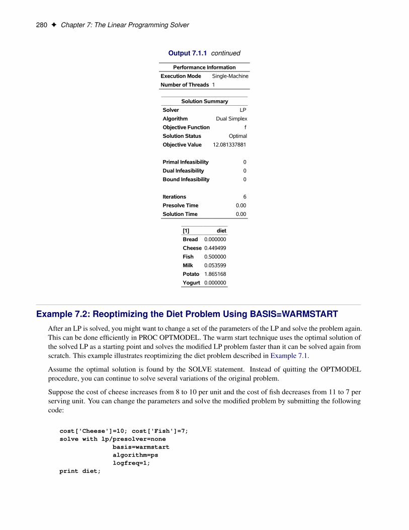
The optimal solution and the optimal objective value are displayed in Output 7.1.1.
Output 7.1.1 Optimal Solution to the Diet Problem
The OPTMODEL ProcedureThe OPTMODEL Procedure
Problem Summary
Objective Sense Minimization
Objective Function f
Objective Type Linear
Number of Variables 6
Bounded Above 0
Bounded Below 5
Bounded Below and Above 1
Free 0
Fixed 0
Number of Constraints 4
Linear LE (<=) 1
Linear EQ (=) 0
Linear GE (>=) 3
Linear Range 0
Constraint Coefficients 23
280 F Chapter 7: The Linear Programming Solver
Output 7.1.1 continued
Performance Information
Execution Mode Single-Machine
Number of Threads 1
Solution Summary
Solver LP
Algorithm Dual Simplex
Objective Function f
Solution Status Optimal
Objective Value 12.081337881
Primal Infeasibility 0
Dual Infeasibility 0
Bound Infeasibility 0
Iterations 6
Presolve Time 0.00
Solution Time 0.00
[1] diet
Bread 0.000000
Cheese 0.449499
Fish 0.500000
Milk 0.053599
Potato 1.865168
Yogurt 0.000000
Example 7.2: Reoptimizing the Diet Problem Using BASIS=WARMSTARTAfter an LP is solved, you might want to change a set of the parameters of the LP and solve the problem again.This can be done efficiently in PROC OPTMODEL. The warm start technique uses the optimal solution ofthe solved LP as a starting point and solves the modified LP problem faster than it can be solved again fromscratch. This example illustrates reoptimizing the diet problem described in Example 7.1.
Assume the optimal solution is found by the SOLVE statement. Instead of quitting the OPTMODELprocedure, you can continue to solve several variations of the original problem.
Suppose the cost of cheese increases from 8 to 10 per unit and the cost of fish decreases from 11 to 7 perserving unit. You can change the parameters and solve the modified problem by submitting the followingcode:
cost['Cheese']=10; cost['Fish']=7;solve with lp/presolver=none
basis=warmstartalgorithm=pslogfreq=1;
print diet;
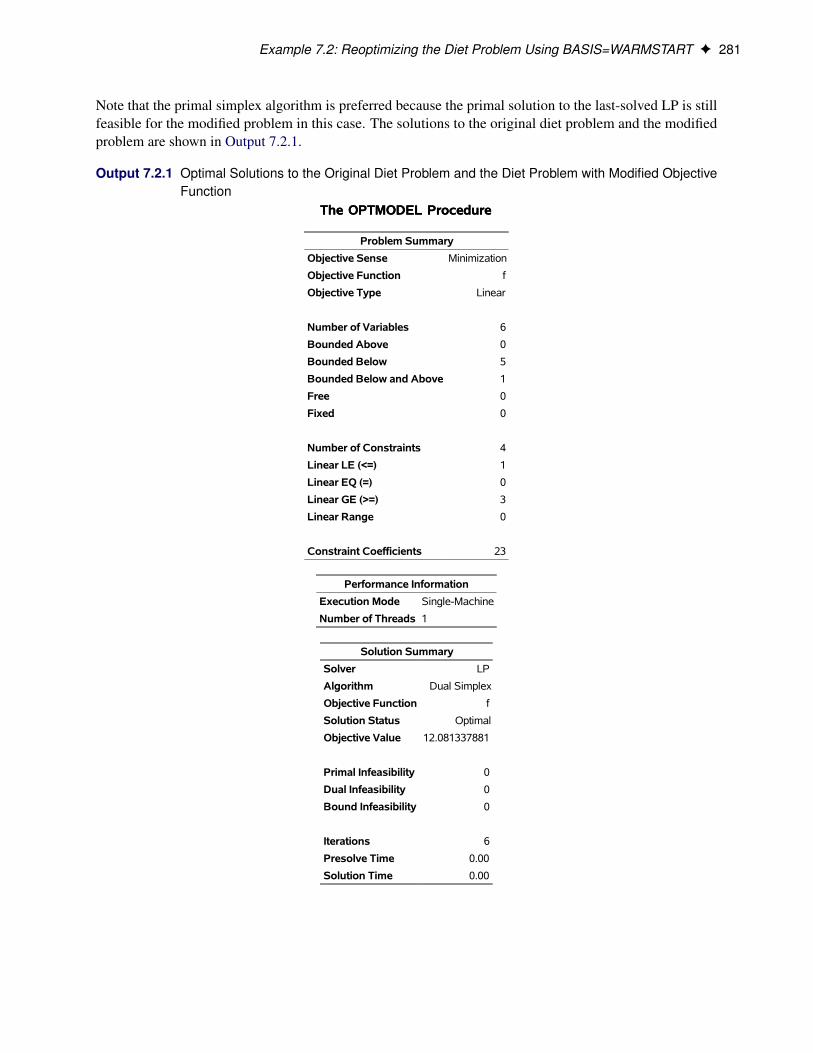
Example 7.2: Reoptimizing the Diet Problem Using BASIS=WARMSTART F 281
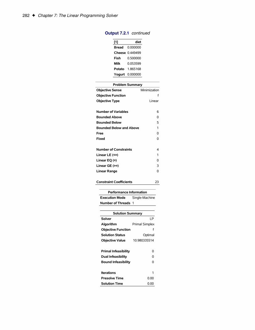
Note that the primal simplex algorithm is preferred because the primal solution to the last-solved LP is stillfeasible for the modified problem in this case. The solutions to the original diet problem and the modifiedproblem are shown in Output 7.2.1.
Output 7.2.1 Optimal Solutions to the Original Diet Problem and the Diet Problem with Modified ObjectiveFunction
The OPTMODEL ProcedureThe OPTMODEL Procedure
Problem Summary
Objective Sense Minimization
Objective Function f
Objective Type Linear
Number of Variables 6
Bounded Above 0
Bounded Below 5
Bounded Below and Above 1
Free 0
Fixed 0
Number of Constraints 4
Linear LE (<=) 1
Linear EQ (=) 0
Linear GE (>=) 3
Linear Range 0
Constraint Coefficients 23
Performance Information
Execution Mode Single-Machine
Number of Threads 1
Solution Summary
Solver LP
Algorithm Dual Simplex
Objective Function f
Solution Status Optimal
Objective Value 12.081337881
Primal Infeasibility 0
Dual Infeasibility 0
Bound Infeasibility 0
Iterations 6
Presolve Time 0.00
Solution Time 0.00
282 F Chapter 7: The Linear Programming Solver
Output 7.2.1 continued
[1] diet
Bread 0.000000
Cheese 0.449499
Fish 0.500000
Milk 0.053599
Potato 1.865168
Yogurt 0.000000
Problem Summary
Objective Sense Minimization
Objective Function f
Objective Type Linear
Number of Variables 6
Bounded Above 0
Bounded Below 5
Bounded Below and Above 1
Free 0
Fixed 0
Number of Constraints 4
Linear LE (<=) 1
Linear EQ (=) 0
Linear GE (>=) 3
Linear Range 0
Constraint Coefficients 23
Performance Information
Execution Mode Single-Machine
Number of Threads 1
Solution Summary
Solver LP
Algorithm Primal Simplex
Objective Function f
Solution Status Optimal
Objective Value 10.980335514
Primal Infeasibility 0
Dual Infeasibility 0
Bound Infeasibility 0
Iterations 1
Presolve Time 0.00
Solution Time 0.00
Example 7.2: Reoptimizing the Diet Problem Using BASIS=WARMSTART F 283
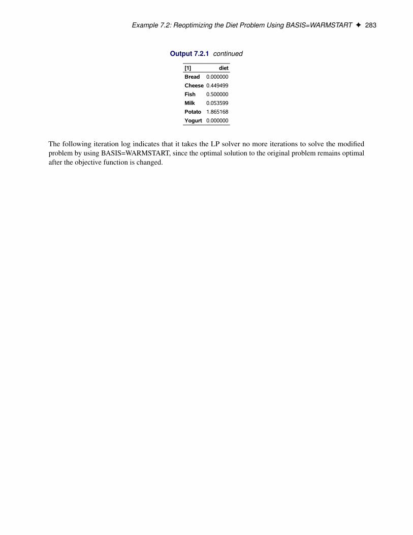
Output 7.2.1 continued
[1] diet
Bread 0.000000
Cheese 0.449499
Fish 0.500000
Milk 0.053599
Potato 1.865168
Yogurt 0.000000
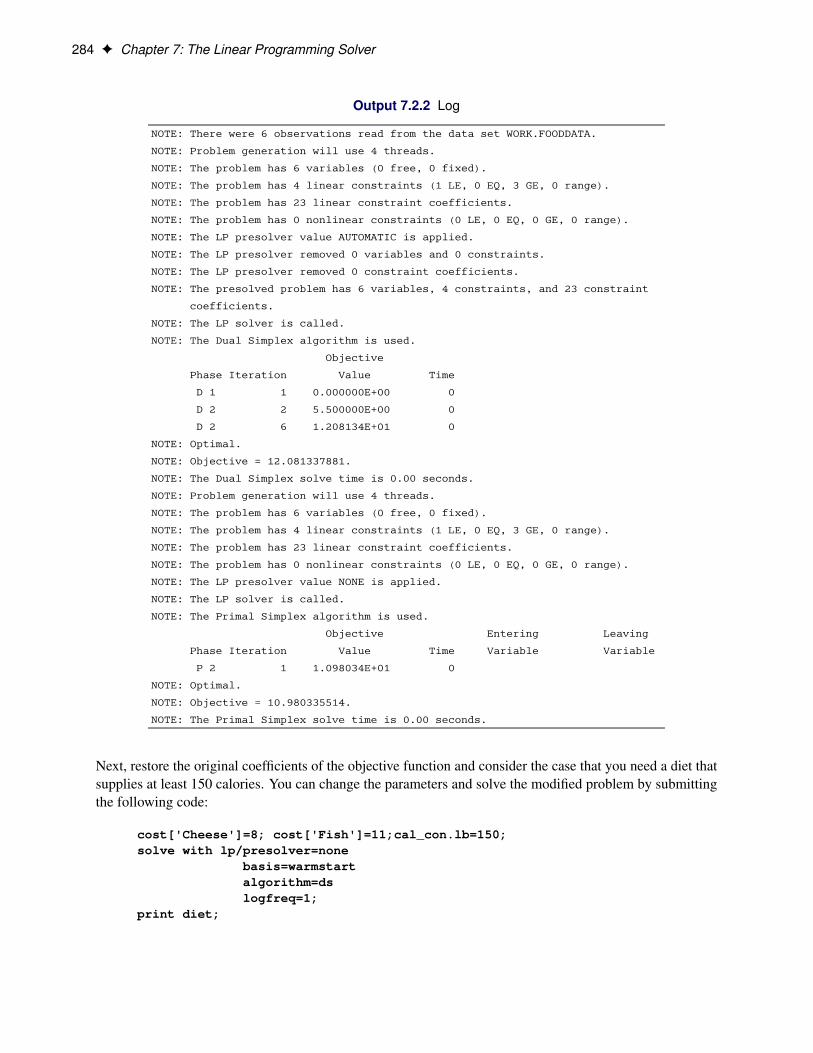
The following iteration log indicates that it takes the LP solver no more iterations to solve the modifiedproblem by using BASIS=WARMSTART, since the optimal solution to the original problem remains optimalafter the objective function is changed.
284 F Chapter 7: The Linear Programming Solver
Output 7.2.2 Log
NOTE: There were 6 observations read from the data set WORK.FOODDATA.
NOTE: Problem generation will use 4 threads.
NOTE: The problem has 6 variables (0 free, 0 fixed).
NOTE: The problem has 4 linear constraints (1 LE, 0 EQ, 3 GE, 0 range).
NOTE: The problem has 23 linear constraint coefficients.
NOTE: The problem has 0 nonlinear constraints (0 LE, 0 EQ, 0 GE, 0 range).
NOTE: The LP presolver value AUTOMATIC is applied.
NOTE: The LP presolver removed 0 variables and 0 constraints.
NOTE: The LP presolver removed 0 constraint coefficients.
NOTE: The presolved problem has 6 variables, 4 constraints, and 23 constraint
coefficients.
NOTE: The LP solver is called.
NOTE: The Dual Simplex algorithm is used.
Objective
Phase Iteration Value Time
D 1 1 0.000000E+00 0
D 2 2 5.500000E+00 0
D 2 6 1.208134E+01 0
NOTE: Optimal.
NOTE: Objective = 12.081337881.
NOTE: The Dual Simplex solve time is 0.00 seconds.
NOTE: Problem generation will use 4 threads.
NOTE: The problem has 6 variables (0 free, 0 fixed).
NOTE: The problem has 4 linear constraints (1 LE, 0 EQ, 3 GE, 0 range).
NOTE: The problem has 23 linear constraint coefficients.
NOTE: The problem has 0 nonlinear constraints (0 LE, 0 EQ, 0 GE, 0 range).
NOTE: The LP presolver value NONE is applied.
NOTE: The LP solver is called.
NOTE: The Primal Simplex algorithm is used.
Objective Entering Leaving
Phase Iteration Value Time Variable Variable
P 2 1 1.098034E+01 0
NOTE: Optimal.
NOTE: Objective = 10.980335514.
NOTE: The Primal Simplex solve time is 0.00 seconds.
Next, restore the original coefficients of the objective function and consider the case that you need a diet thatsupplies at least 150 calories. You can change the parameters and solve the modified problem by submittingthe following code:
cost['Cheese']=8; cost['Fish']=11;cal_con.lb=150;solve with lp/presolver=none
basis=warmstartalgorithm=dslogfreq=1;
print diet;
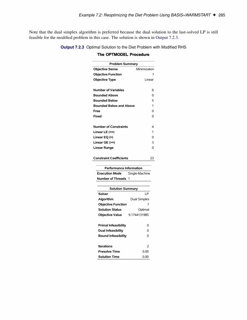
Example 7.2: Reoptimizing the Diet Problem Using BASIS=WARMSTART F 285
Note that the dual simplex algorithm is preferred because the dual solution to the last-solved LP is stillfeasible for the modified problem in this case. The solution is shown in Output 7.2.3.
Output 7.2.3 Optimal Solution to the Diet Problem with Modified RHS
The OPTMODEL ProcedureThe OPTMODEL Procedure
Problem Summary
Objective Sense Minimization
Objective Function f
Objective Type Linear
Number of Variables 6
Bounded Above 0
Bounded Below 5
Bounded Below and Above 1
Free 0
Fixed 0
Number of Constraints 4
Linear LE (<=) 1
Linear EQ (=) 0
Linear GE (>=) 3
Linear Range 0
Constraint Coefficients 23
Performance Information
Execution Mode Single-Machine
Number of Threads 1
Solution Summary
Solver LP
Algorithm Dual Simplex
Objective Function f
Solution Status Optimal
Objective Value 9.1744131985
Primal Infeasibility 0
Dual Infeasibility 0
Bound Infeasibility 0
Iterations 2
Presolve Time 0.00
Solution Time 0.00
286 F Chapter 7: The Linear Programming Solver
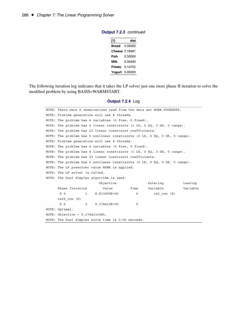
Output 7.2.3 continued
[1] diet
Bread 0.00000
Cheese 0.18481
Fish 0.50000
Milk 0.56440
Potato 0.14702
Yogurt 0.00000
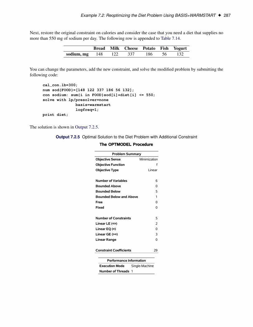
The following iteration log indicates that it takes the LP solver just one more phase II iteration to solve themodified problem by using BASIS=WARMSTART.
Output 7.2.4 Log
NOTE: There were 6 observations read from the data set WORK.FOODDATA.
NOTE: Problem generation will use 4 threads.
NOTE: The problem has 6 variables (0 free, 0 fixed).
NOTE: The problem has 4 linear constraints (1 LE, 0 EQ, 3 GE, 0 range).
NOTE: The problem has 23 linear constraint coefficients.
NOTE: The problem has 0 nonlinear constraints (0 LE, 0 EQ, 0 GE, 0 range).
NOTE: The LP presolver value NONE is applied.
NOTE: The LP solver is called.
NOTE: The Dual Simplex algorithm is used.
Objective Entering Leaving
Phase Iteration Value Time Variable Variable
D 2 1 8.813205E+00 0 cal_con (S)
carb_con (S)
D 2 2 9.174413E+00 0
NOTE: Optimal.
NOTE: Objective = 9.1744131985.
NOTE: The Dual Simplex solve time is 0.00 seconds.
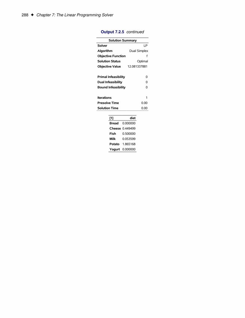
Example 7.2: Reoptimizing the Diet Problem Using BASIS=WARMSTART F 287
Next, restore the original constraint on calories and consider the case that you need a diet that supplies nomore than 550 mg of sodium per day. The following row is appended to Table 7.14.
Bread Milk Cheese Potato Fish Yogurtsodium, mg 148 122 337 186 56 132
You can change the parameters, add the new constraint, and solve the modified problem by submitting thefollowing code:
cal_con.lb=300;num sod{FOOD}=[148 122 337 186 56 132];con sodium: sum{i in FOOD}sod[i]*diet[i] <= 550;solve with lp/presolver=none
basis=warmstartlogfreq=1;
print diet;
The solution is shown in Output 7.2.5.
Output 7.2.5 Optimal Solution to the Diet Problem with Additional Constraint
The OPTMODEL ProcedureThe OPTMODEL Procedure
Problem Summary
Objective Sense Minimization
Objective Function f
Objective Type Linear
Number of Variables 6
Bounded Above 0
Bounded Below 5
Bounded Below and Above 1
Free 0
Fixed 0
Number of Constraints 5
Linear LE (<=) 2
Linear EQ (=) 0
Linear GE (>=) 3
Linear Range 0
Constraint Coefficients 29
Performance Information
Execution Mode Single-Machine
Number of Threads 1
288 F Chapter 7: The Linear Programming Solver
Output 7.2.5 continued
Solution Summary
Solver LP
Algorithm Dual Simplex
Objective Function f
Solution Status Optimal
Objective Value 12.081337881
Primal Infeasibility 0
Dual Infeasibility 0
Bound Infeasibility 0
Iterations 1
Presolve Time 0.00
Solution Time 0.00
[1] diet
Bread 0.000000
Cheese 0.449499
Fish 0.500000
Milk 0.053599
Potato 1.865168
Yogurt 0.000000
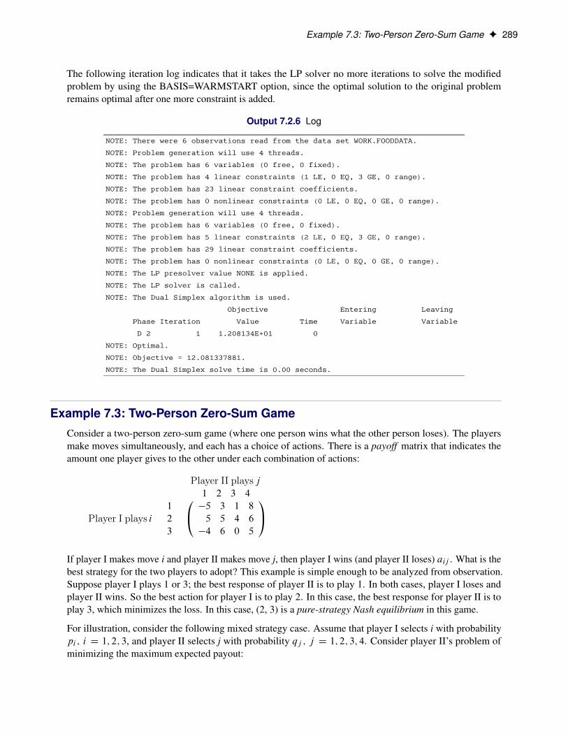
Example 7.3: Two-Person Zero-Sum Game F 289
The following iteration log indicates that it takes the LP solver no more iterations to solve the modifiedproblem by using the BASIS=WARMSTART option, since the optimal solution to the original problemremains optimal after one more constraint is added.
Output 7.2.6 Log
NOTE: There were 6 observations read from the data set WORK.FOODDATA.
NOTE: Problem generation will use 4 threads.
NOTE: The problem has 6 variables (0 free, 0 fixed).
NOTE: The problem has 4 linear constraints (1 LE, 0 EQ, 3 GE, 0 range).
NOTE: The problem has 23 linear constraint coefficients.
NOTE: The problem has 0 nonlinear constraints (0 LE, 0 EQ, 0 GE, 0 range).
NOTE: Problem generation will use 4 threads.
NOTE: The problem has 6 variables (0 free, 0 fixed).
NOTE: The problem has 5 linear constraints (2 LE, 0 EQ, 3 GE, 0 range).
NOTE: The problem has 29 linear constraint coefficients.
NOTE: The problem has 0 nonlinear constraints (0 LE, 0 EQ, 0 GE, 0 range).
NOTE: The LP presolver value NONE is applied.
NOTE: The LP solver is called.
NOTE: The Dual Simplex algorithm is used.
Objective Entering Leaving
Phase Iteration Value Time Variable Variable
D 2 1 1.208134E+01 0
NOTE: Optimal.
NOTE: Objective = 12.081337881.
NOTE: The Dual Simplex solve time is 0.00 seconds.
Example 7.3: Two-Person Zero-Sum GameConsider a two-person zero-sum game (where one person wins what the other person loses). The playersmake moves simultaneously, and each has a choice of actions. There is a payoff matrix that indicates theamount one player gives to the other under each combination of actions:
Player II plays j1 2 3 4
Player I plays i1
2
3
0@ �5 3 1 8
5 5 4 6
�4 6 0 5
1AIf player I makes move i and player II makes move j, then player I wins (and player II loses) aij . What is thebest strategy for the two players to adopt? This example is simple enough to be analyzed from observation.Suppose player I plays 1 or 3; the best response of player II is to play 1. In both cases, player I loses andplayer II wins. So the best action for player I is to play 2. In this case, the best response for player II is toplay 3, which minimizes the loss. In this case, (2, 3) is a pure-strategy Nash equilibrium in this game.
For illustration, consider the following mixed strategy case. Assume that player I selects i with probabilitypi ; i D 1; 2; 3, and player II selects j with probability qj ; j D 1; 2; 3; 4. Consider player II’s problem ofminimizing the maximum expected payout:
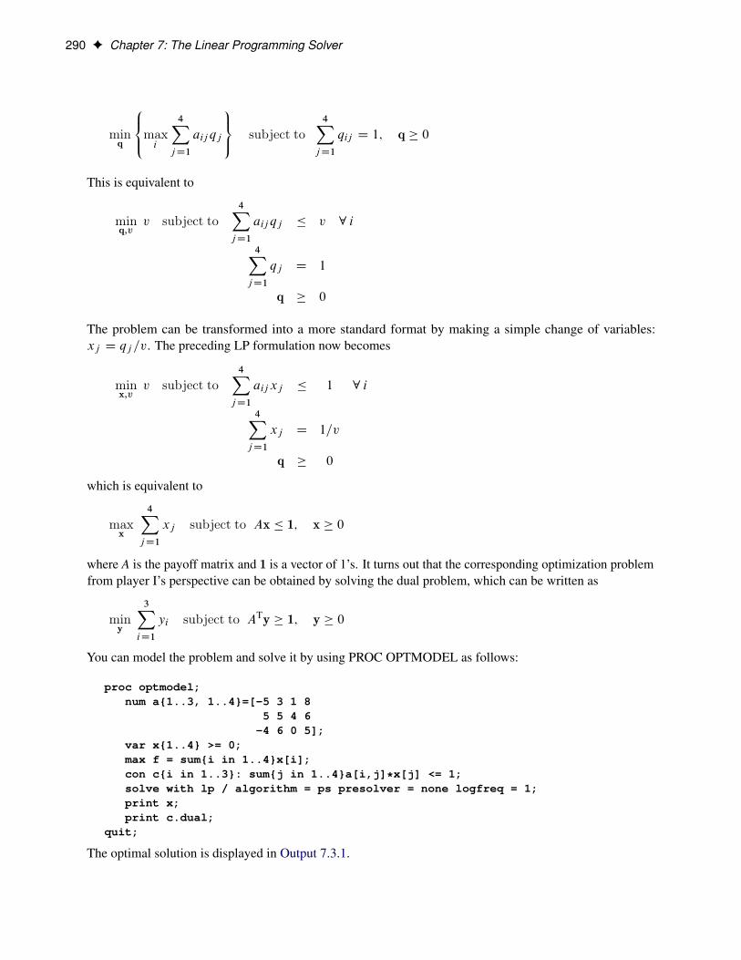
290 F Chapter 7: The Linear Programming Solver
minq
8<:maxi
4XjD1
aij qj
9=; subject to4X
jD1
qij D 1; q � 0
This is equivalent to
minq;v
v subject to4X
jD1
aij qj � v 8 i
4XjD1
qj D 1
q � 0
The problem can be transformed into a more standard format by making a simple change of variables:xj D qj =v. The preceding LP formulation now becomes
minx;v
v subject to4X
jD1
aijxj � 1 8 i
4XjD1
xj D 1=v
q � 0
which is equivalent to
maxx
4XjD1
xj subject to Ax � 1; x � 0
where A is the payoff matrix and 1 is a vector of 1’s. It turns out that the corresponding optimization problemfrom player I’s perspective can be obtained by solving the dual problem, which can be written as
miny
3XiD1
yi subject to ATy � 1; y � 0
You can model the problem and solve it by using PROC OPTMODEL as follows:
proc optmodel;num a{1..3, 1..4}=[-5 3 1 8
5 5 4 6-4 6 0 5];
var x{1..4} >= 0;max f = sum{i in 1..4}x[i];con c{i in 1..3}: sum{j in 1..4}a[i,j]*x[j] <= 1;solve with lp / algorithm = ps presolver = none logfreq = 1;print x;print c.dual;
quit;
The optimal solution is displayed in Output 7.3.1.
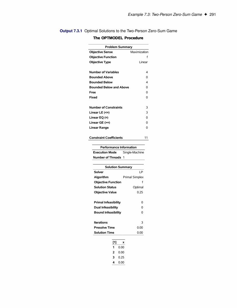
Example 7.3: Two-Person Zero-Sum Game F 291
Output 7.3.1 Optimal Solutions to the Two-Person Zero-Sum Game
The OPTMODEL ProcedureThe OPTMODEL Procedure
Problem Summary
Objective Sense Maximization
Objective Function f
Objective Type Linear
Number of Variables 4
Bounded Above 0
Bounded Below 4
Bounded Below and Above 0
Free 0
Fixed 0
Number of Constraints 3
Linear LE (<=) 3
Linear EQ (=) 0
Linear GE (>=) 0
Linear Range 0
Constraint Coefficients 11
Performance Information
Execution Mode Single-Machine
Number of Threads 1
Solution Summary
Solver LP
Algorithm Primal Simplex
Objective Function f
Solution Status Optimal
Objective Value 0.25
Primal Infeasibility 0
Dual Infeasibility 0
Bound Infeasibility 0
Iterations 3
Presolve Time 0.00
Solution Time 0.00
[1] x
1 0.00
2 0.00
3 0.25
4 0.00
292 F Chapter 7: The Linear Programming Solver
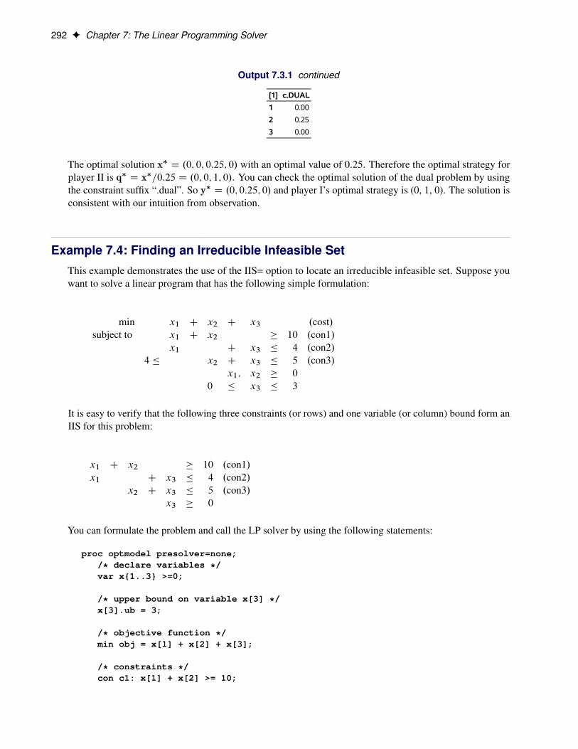
Output 7.3.1 continued
[1] c.DUAL
1 0.00
2 0.25
3 0.00
The optimal solution x� D .0; 0; 0:25; 0/ with an optimal value of 0.25. Therefore the optimal strategy forplayer II is q� D x�=0:25 D .0; 0; 1; 0/. You can check the optimal solution of the dual problem by usingthe constraint suffix “.dual”. So y� D .0; 0:25; 0/ and player I’s optimal strategy is (0, 1, 0). The solution isconsistent with our intuition from observation.
Example 7.4: Finding an Irreducible Infeasible SetThis example demonstrates the use of the IIS= option to locate an irreducible infeasible set. Suppose youwant to solve a linear program that has the following simple formulation:
min x1 C x2 C x3 .cost/subject to x1 C x2 � 10 .con1/
x1 C x3 � 4 .con2/4 � x2 C x3 � 5 .con3/
x1; x2 � 0
0 � x3 � 3
It is easy to verify that the following three constraints (or rows) and one variable (or column) bound form anIIS for this problem:
x1 C x2 � 10 .con1/x1 C x3 � 4 .con2/
x2 C x3 � 5 .con3/x3 � 0
You can formulate the problem and call the LP solver by using the following statements:
proc optmodel presolver=none;/* declare variables */var x{1..3} >=0;
/* upper bound on variable x[3] */x[3].ub = 3;
/* objective function */min obj = x[1] + x[2] + x[3];
/* constraints */con c1: x[1] + x[2] >= 10;
Example 7.4: Finding an Irreducible Infeasible Set F 293
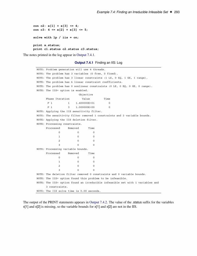
con c2: x[1] + x[3] <= 4;con c3: 4 <= x[2] + x[3] <= 5;
solve with lp / iis = on;
print x.status;print c1.status c2.status c3.status;
The notes printed in the log appear in Output 7.4.1.
Output 7.4.1 Finding an IIS: Log
NOTE: Problem generation will use 4 threads.
NOTE: The problem has 3 variables (0 free, 0 fixed).
NOTE: The problem has 3 linear constraints (1 LE, 0 EQ, 1 GE, 1 range).
NOTE: The problem has 6 linear constraint coefficients.
NOTE: The problem has 0 nonlinear constraints (0 LE, 0 EQ, 0 GE, 0 range).
NOTE: The IIS= option is enabled.
Objective
Phase Iteration Value Time
P 1 1 1.400000E+01 0
P 1 3 1.000000E+00 0
NOTE: Applying the IIS sensitivity filter.
NOTE: The sensitivity filter removed 1 constraints and 3 variable bounds.
NOTE: Applying the IIS deletion filter.
NOTE: Processing constraints.
Processed Removed Time
0 0 0
1 0 0
2 0 0
3 0 0
NOTE: Processing variable bounds.
Processed Removed Time
0 0 0
1 0 0
2 0 0
3 0 0
NOTE: The deletion filter removed 0 constraints and 0 variable bounds.
NOTE: The IIS= option found this problem to be infeasible.
NOTE: The IIS= option found an irreducible infeasible set with 1 variables and
3 constraints.
NOTE: The IIS solve time is 0.00 seconds.
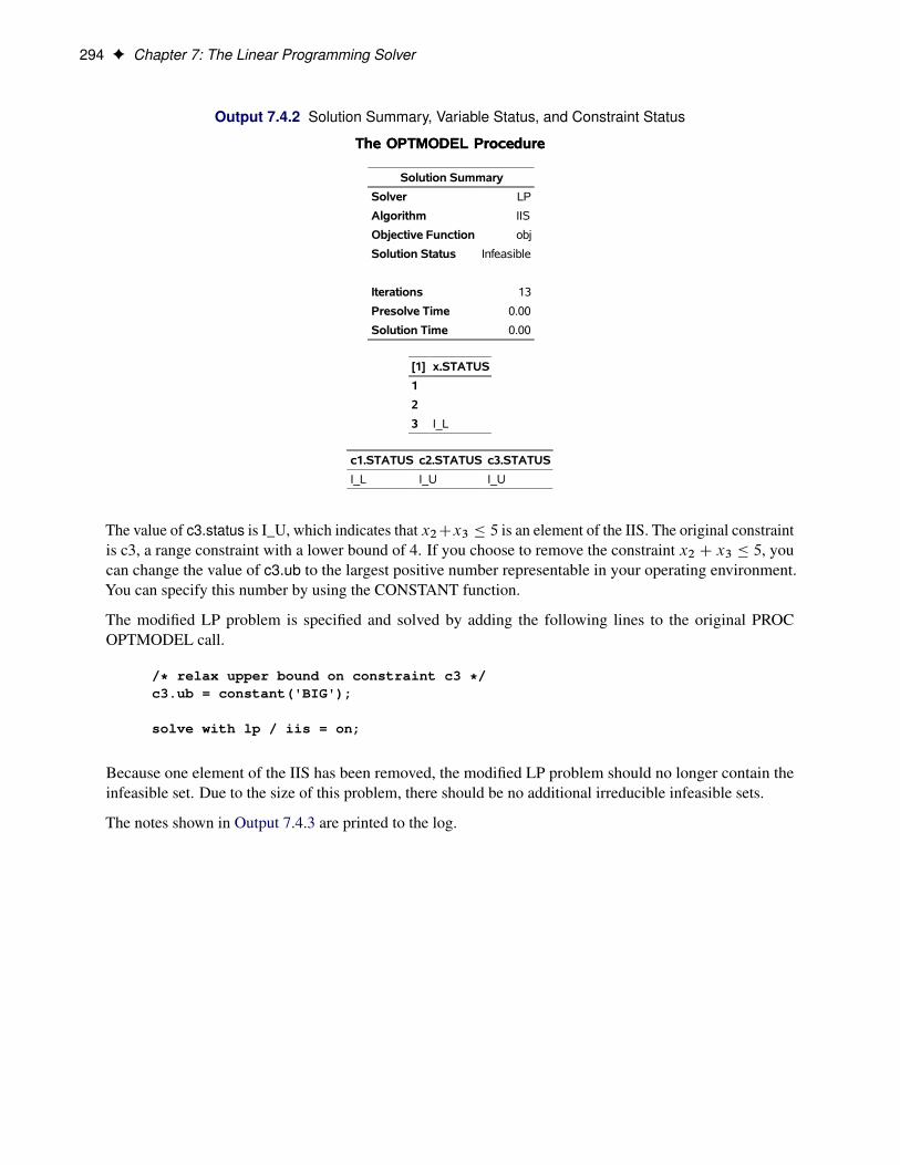
The output of the PRINT statements appears in Output 7.4.2. The value of the .status suffix for the variablesx[1] and x[2] is missing, so the variable bounds for x[1] and x[2] are not in the IIS.
294 F Chapter 7: The Linear Programming Solver
Output 7.4.2 Solution Summary, Variable Status, and Constraint Status
The OPTMODEL ProcedureThe OPTMODEL Procedure
Solution Summary
Solver LP
Algorithm IIS
Objective Function obj
Solution Status Infeasible
Iterations 13
Presolve Time 0.00
Solution Time 0.00
[1] x.STATUS
1
2
3 I_L
c1.STATUS c2.STATUS c3.STATUS
I_L I_U I_U
The value of c3.status is I_U, which indicates that x2Cx3 � 5 is an element of the IIS. The original constraintis c3, a range constraint with a lower bound of 4. If you choose to remove the constraint x2 C x3 � 5, youcan change the value of c3.ub to the largest positive number representable in your operating environment.You can specify this number by using the CONSTANT function.
The modified LP problem is specified and solved by adding the following lines to the original PROCOPTMODEL call.
/* relax upper bound on constraint c3 */c3.ub = constant('BIG');
solve with lp / iis = on;
Because one element of the IIS has been removed, the modified LP problem should no longer contain theinfeasible set. Due to the size of this problem, there should be no additional irreducible infeasible sets.
The notes shown in Output 7.4.3 are printed to the log.
Example 7.5: Using the Network Simplex Algorithm F 295
Output 7.4.3 Infeasibility Removed: Log
NOTE: Problem generation will use 4 threads.
NOTE: The problem has 3 variables (0 free, 0 fixed).
NOTE: The problem has 3 linear constraints (1 LE, 0 EQ, 2 GE, 0 range).
NOTE: The problem has 6 linear constraint coefficients.
NOTE: The problem has 0 nonlinear constraints (0 LE, 0 EQ, 0 GE, 0 range).
NOTE: The IIS= option is enabled.
Objective
Phase Iteration Value Time
P 1 1 1.400000E+01 0
P 1 3 0.000000E+00 0
NOTE: The IIS= option found this problem to be feasible.
NOTE: The IIS solve time is 0.00 seconds.
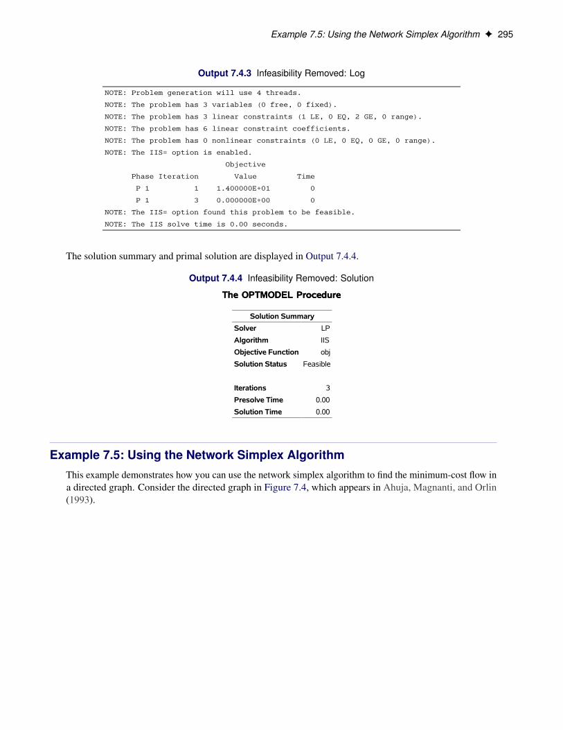
The solution summary and primal solution are displayed in Output 7.4.4.
Output 7.4.4 Infeasibility Removed: Solution
The OPTMODEL ProcedureThe OPTMODEL Procedure
Solution Summary
Solver LP
Algorithm IIS
Objective Function obj
Solution Status Feasible
Iterations 3
Presolve Time 0.00
Solution Time 0.00
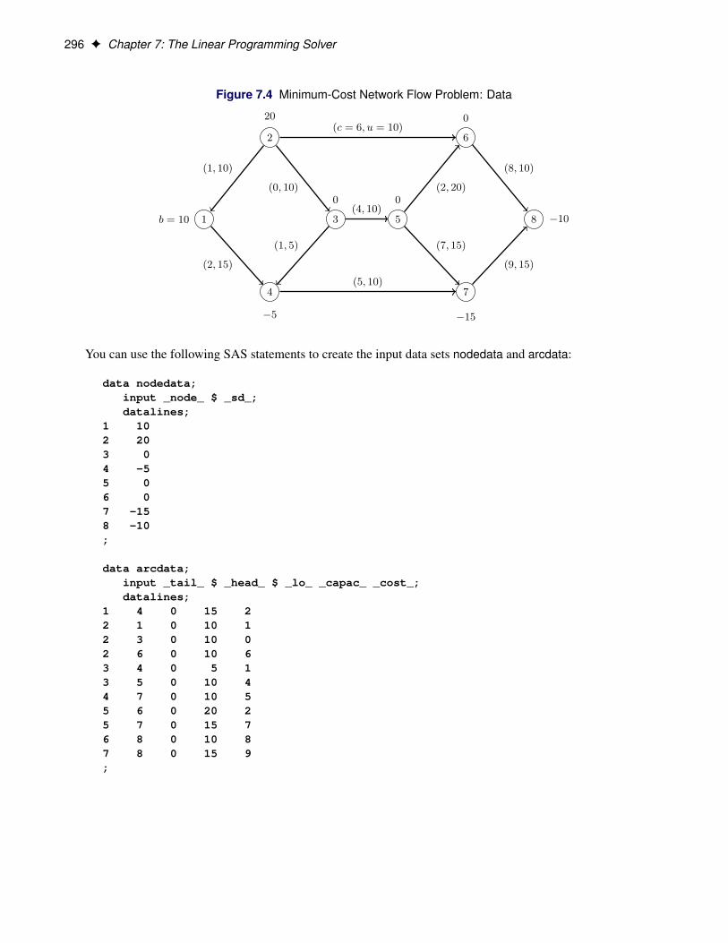
Example 7.5: Using the Network Simplex AlgorithmThis example demonstrates how you can use the network simplex algorithm to find the minimum-cost flow ina directed graph. Consider the directed graph in Figure 7.4, which appears in Ahuja, Magnanti, and Orlin(1993).
296 F Chapter 7: The Linear Programming Solver
Figure 7.4 Minimum-Cost Network Flow Problem: Data
2
20
6
0
1b = 10 3
0
5
0
8 −10
4
−5
7
−15
(2, 15)
(1, 10)
(0, 10)
(c = 6, u = 10)
(1, 5)
(4, 10)
(5, 10)
(2, 20)
(7, 15)
(8, 10)
(9, 15)
You can use the following SAS statements to create the input data sets nodedata and arcdata:
data nodedata;input _node_ $ _sd_;datalines;
1 102 203 04 -55 06 07 -158 -10;
data arcdata;input _tail_ $ _head_ $ _lo_ _capac_ _cost_;datalines;
1 4 0 15 22 1 0 10 12 3 0 10 02 6 0 10 63 4 0 5 13 5 0 10 44 7 0 10 55 6 0 20 25 7 0 15 76 8 0 10 87 8 0 15 9;
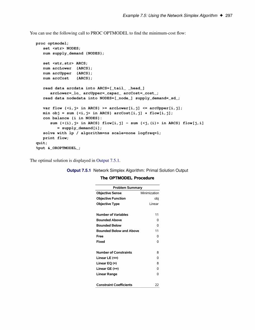
Example 7.5: Using the Network Simplex Algorithm F 297
You can use the following call to PROC OPTMODEL to find the minimum-cost flow:
proc optmodel;set <str> NODES;num supply_demand {NODES};
set <str,str> ARCS;num arcLower {ARCS};num arcUpper {ARCS};num arcCost {ARCS};
read data arcdata into ARCS=[_tail_ _head_]arcLower=_lo_ arcUpper=_capac_ arcCost=_cost_;
read data nodedata into NODES=[_node_] supply_demand=_sd_;
var flow {<i,j> in ARCS} >= arcLower[i,j] <= arcUpper[i,j];min obj = sum {<i,j> in ARCS} arcCost[i,j] * flow[i,j];con balance {i in NODES}:
sum {<(i),j> in ARCS} flow[i,j] - sum {<j,(i)> in ARCS} flow[j,i]= supply_demand[i];
solve with lp / algorithm=ns scale=none logfreq=1;print flow;
quit;%put &_OROPTMODEL_;
The optimal solution is displayed in Output 7.5.1.
Output 7.5.1 Network Simplex Algorithm: Primal Solution Output
The OPTMODEL ProcedureThe OPTMODEL Procedure
Problem Summary
Objective Sense Minimization
Objective Function obj
Objective Type Linear
Number of Variables 11
Bounded Above 0
Bounded Below 0
Bounded Below and Above 11
Free 0
Fixed 0
Number of Constraints 8
Linear LE (<=) 0
Linear EQ (=) 8
Linear GE (>=) 0
Linear Range 0
Constraint Coefficients 22
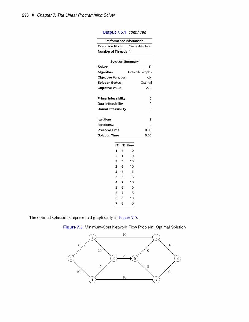
298 F Chapter 7: The Linear Programming Solver
Output 7.5.1 continued
Performance Information
Execution Mode Single-Machine
Number of Threads 1
Solution Summary
Solver LP
Algorithm Network Simplex
Objective Function obj
Solution Status Optimal
Objective Value 270
Primal Infeasibility 0
Dual Infeasibility 0
Bound Infeasibility 0
Iterations 8
Iterations2 0
Presolve Time 0.00
Solution Time 0.00
[1] [2] flow
1 4 10
2 1 0
2 3 10
2 6 10
3 4 5
3 5 5
4 7 10
5 6 0
5 7 5
6 8 10
7 8 0
The optimal solution is represented graphically in Figure 7.5.
Figure 7.5 Minimum-Cost Network Flow Problem: Optimal Solution
2 6
1 3 5 8
4 7
10
0
10
10
5
5
10
0
5
10
0
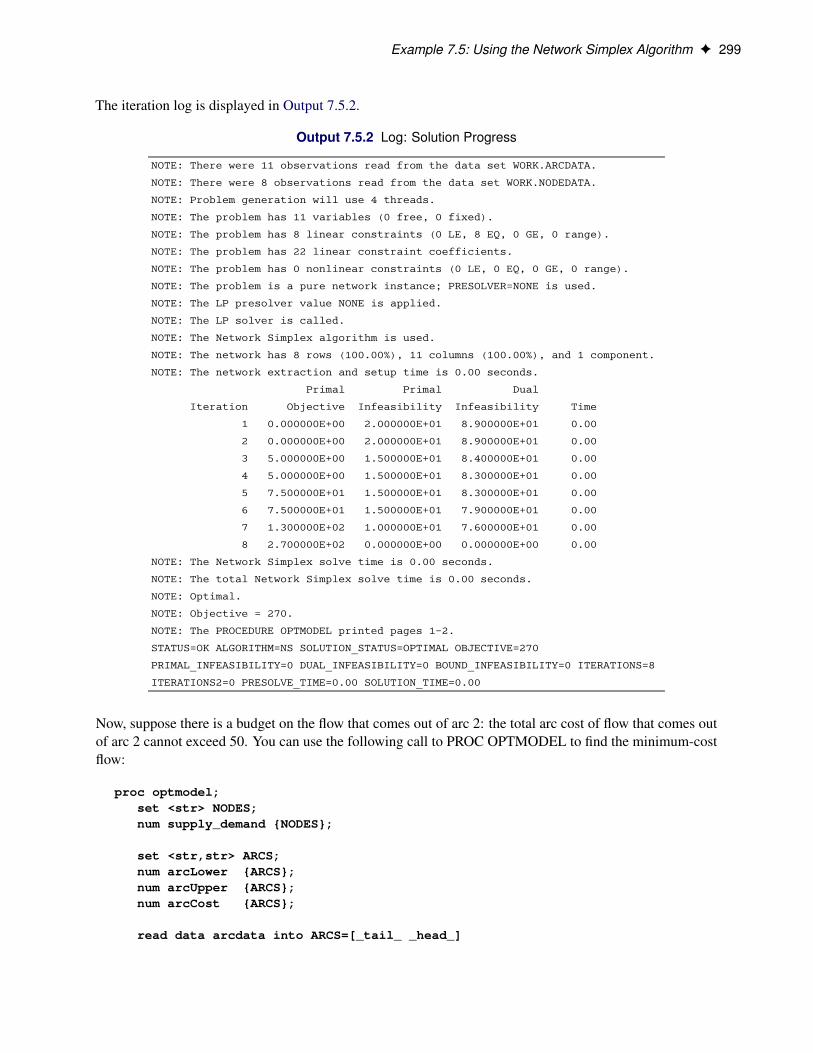
Example 7.5: Using the Network Simplex Algorithm F 299
The iteration log is displayed in Output 7.5.2.
Output 7.5.2 Log: Solution Progress
NOTE: There were 11 observations read from the data set WORK.ARCDATA.
NOTE: There were 8 observations read from the data set WORK.NODEDATA.
NOTE: Problem generation will use 4 threads.
NOTE: The problem has 11 variables (0 free, 0 fixed).
NOTE: The problem has 8 linear constraints (0 LE, 8 EQ, 0 GE, 0 range).
NOTE: The problem has 22 linear constraint coefficients.
NOTE: The problem has 0 nonlinear constraints (0 LE, 0 EQ, 0 GE, 0 range).
NOTE: The problem is a pure network instance; PRESOLVER=NONE is used.
NOTE: The LP presolver value NONE is applied.
NOTE: The LP solver is called.
NOTE: The Network Simplex algorithm is used.
NOTE: The network has 8 rows (100.00%), 11 columns (100.00%), and 1 component.
NOTE: The network extraction and setup time is 0.00 seconds.
Primal Primal Dual
Iteration Objective Infeasibility Infeasibility Time
1 0.000000E+00 2.000000E+01 8.900000E+01 0.00
2 0.000000E+00 2.000000E+01 8.900000E+01 0.00
3 5.000000E+00 1.500000E+01 8.400000E+01 0.00
4 5.000000E+00 1.500000E+01 8.300000E+01 0.00
5 7.500000E+01 1.500000E+01 8.300000E+01 0.00
6 7.500000E+01 1.500000E+01 7.900000E+01 0.00
7 1.300000E+02 1.000000E+01 7.600000E+01 0.00
8 2.700000E+02 0.000000E+00 0.000000E+00 0.00
NOTE: The Network Simplex solve time is 0.00 seconds.
NOTE: The total Network Simplex solve time is 0.00 seconds.
NOTE: Optimal.
NOTE: Objective = 270.
NOTE: The PROCEDURE OPTMODEL printed pages 1-2.
STATUS=OK ALGORITHM=NS SOLUTION_STATUS=OPTIMAL OBJECTIVE=270
PRIMAL_INFEASIBILITY=0 DUAL_INFEASIBILITY=0 BOUND_INFEASIBILITY=0 ITERATIONS=8
ITERATIONS2=0 PRESOLVE_TIME=0.00 SOLUTION_TIME=0.00
Now, suppose there is a budget on the flow that comes out of arc 2: the total arc cost of flow that comes outof arc 2 cannot exceed 50. You can use the following call to PROC OPTMODEL to find the minimum-costflow:
proc optmodel;set <str> NODES;num supply_demand {NODES};
set <str,str> ARCS;num arcLower {ARCS};num arcUpper {ARCS};num arcCost {ARCS};
read data arcdata into ARCS=[_tail_ _head_]
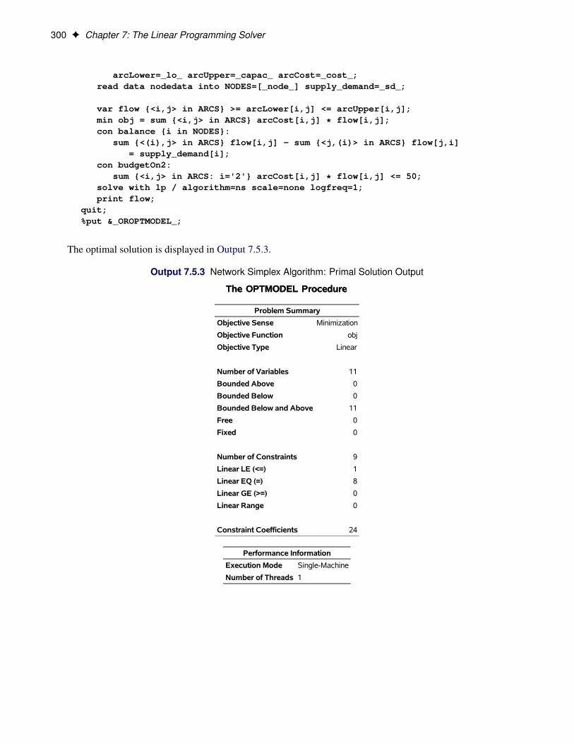
300 F Chapter 7: The Linear Programming Solver
arcLower=_lo_ arcUpper=_capac_ arcCost=_cost_;read data nodedata into NODES=[_node_] supply_demand=_sd_;
var flow {<i,j> in ARCS} >= arcLower[i,j] <= arcUpper[i,j];min obj = sum {<i,j> in ARCS} arcCost[i,j] * flow[i,j];con balance {i in NODES}:
sum {<(i),j> in ARCS} flow[i,j] - sum {<j,(i)> in ARCS} flow[j,i]= supply_demand[i];
con budgetOn2:sum {<i,j> in ARCS: i='2'} arcCost[i,j] * flow[i,j] <= 50;
solve with lp / algorithm=ns scale=none logfreq=1;print flow;
quit;%put &_OROPTMODEL_;
The optimal solution is displayed in Output 7.5.3.
Output 7.5.3 Network Simplex Algorithm: Primal Solution Output
The OPTMODEL ProcedureThe OPTMODEL Procedure
Problem Summary
Objective Sense Minimization
Objective Function obj
Objective Type Linear
Number of Variables 11
Bounded Above 0
Bounded Below 0
Bounded Below and Above 11
Free 0
Fixed 0
Number of Constraints 9
Linear LE (<=) 1
Linear EQ (=) 8
Linear GE (>=) 0
Linear Range 0
Constraint Coefficients 24
Performance Information
Execution Mode Single-Machine
Number of Threads 1
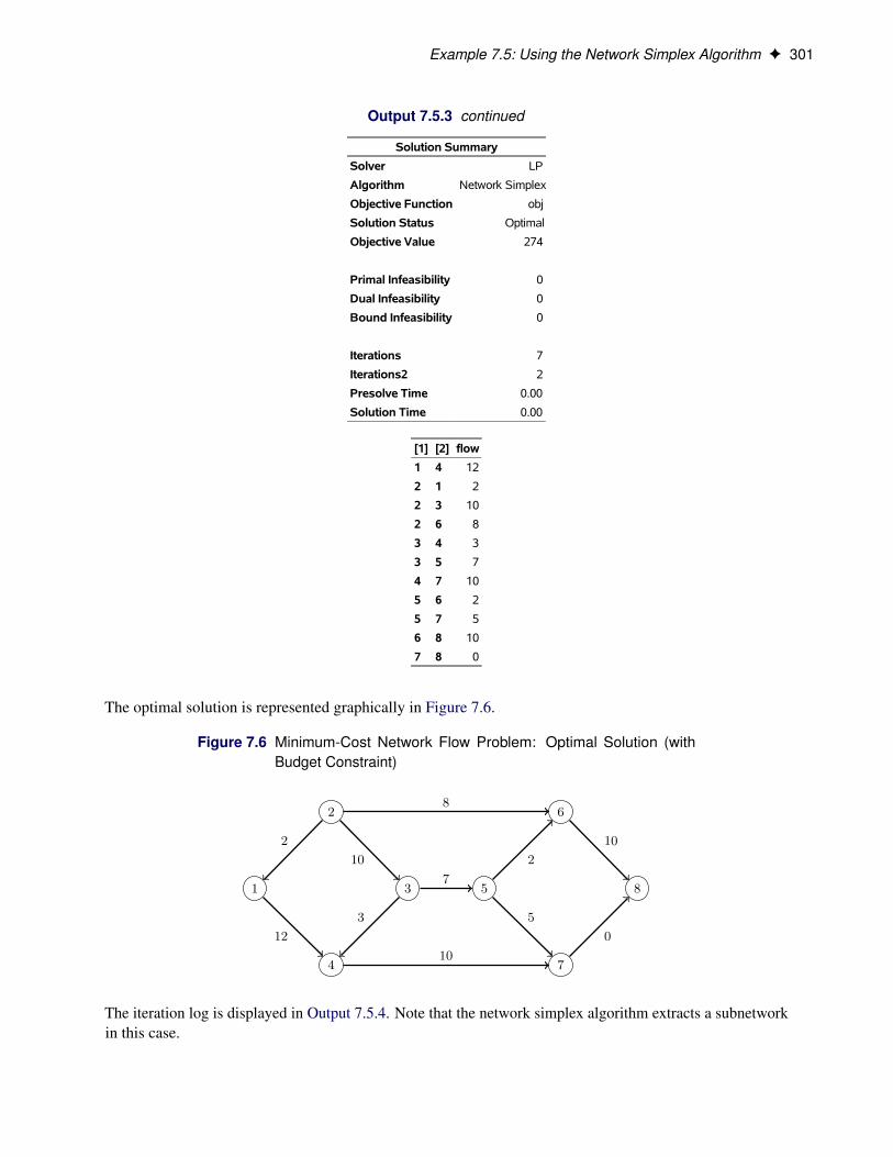
Example 7.5: Using the Network Simplex Algorithm F 301
Output 7.5.3 continued
Solution Summary
Solver LP
Algorithm Network Simplex
Objective Function obj
Solution Status Optimal
Objective Value 274
Primal Infeasibility 0
Dual Infeasibility 0
Bound Infeasibility 0
Iterations 7
Iterations2 2
Presolve Time 0.00
Solution Time 0.00
[1] [2] flow
1 4 12
2 1 2
2 3 10
2 6 8
3 4 3
3 5 7
4 7 10
5 6 2
5 7 5
6 8 10
7 8 0
The optimal solution is represented graphically in Figure 7.6.
Figure 7.6 Minimum-Cost Network Flow Problem: Optimal Solution (withBudget Constraint)
2 6
1 3 5 8
4 7
12
2
10
8
3
7
10
2
5
10
0
The iteration log is displayed in Output 7.5.4. Note that the network simplex algorithm extracts a subnetworkin this case.
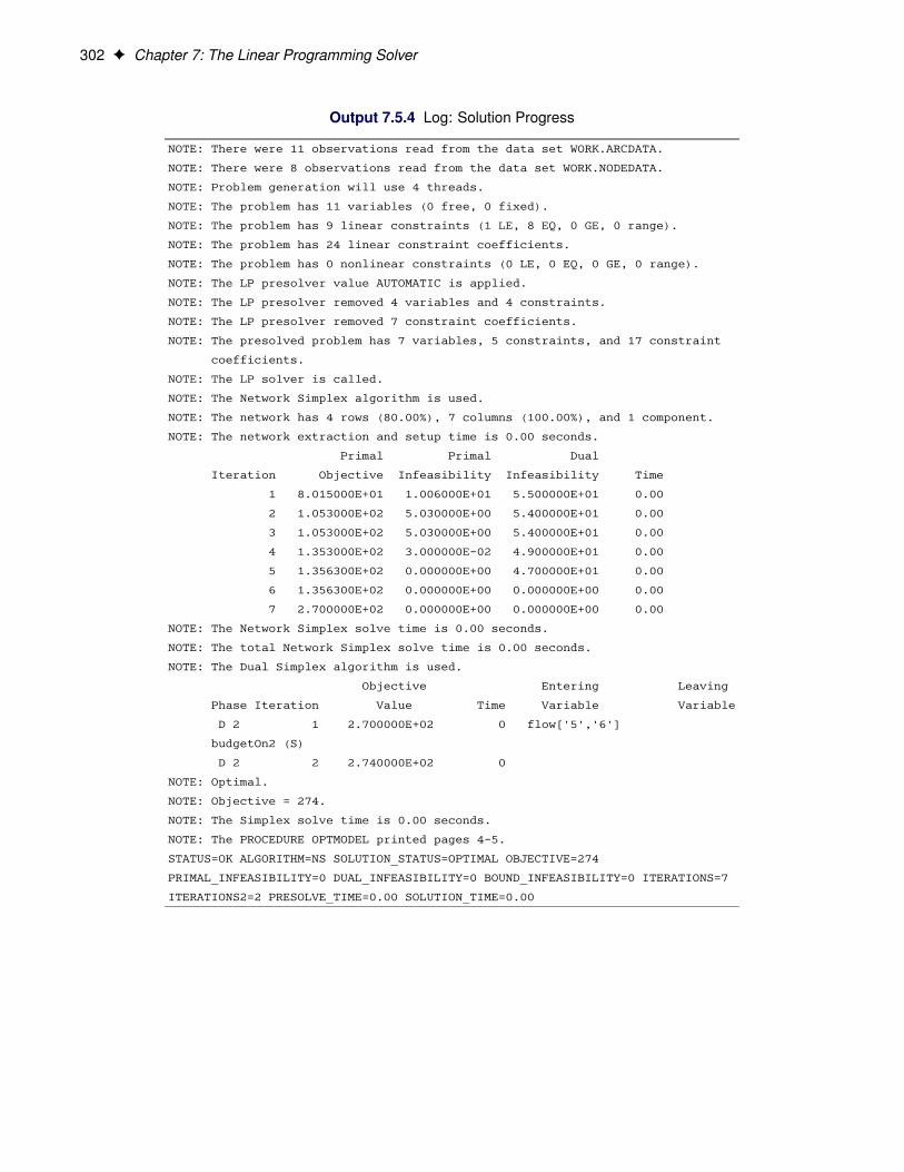
302 F Chapter 7: The Linear Programming Solver
Output 7.5.4 Log: Solution Progress
NOTE: There were 11 observations read from the data set WORK.ARCDATA.
NOTE: There were 8 observations read from the data set WORK.NODEDATA.
NOTE: Problem generation will use 4 threads.
NOTE: The problem has 11 variables (0 free, 0 fixed).
NOTE: The problem has 9 linear constraints (1 LE, 8 EQ, 0 GE, 0 range).
NOTE: The problem has 24 linear constraint coefficients.
NOTE: The problem has 0 nonlinear constraints (0 LE, 0 EQ, 0 GE, 0 range).
NOTE: The LP presolver value AUTOMATIC is applied.
NOTE: The LP presolver removed 4 variables and 4 constraints.
NOTE: The LP presolver removed 7 constraint coefficients.
NOTE: The presolved problem has 7 variables, 5 constraints, and 17 constraint
coefficients.
NOTE: The LP solver is called.
NOTE: The Network Simplex algorithm is used.
NOTE: The network has 4 rows (80.00%), 7 columns (100.00%), and 1 component.
NOTE: The network extraction and setup time is 0.00 seconds.
Primal Primal Dual
Iteration Objective Infeasibility Infeasibility Time
1 8.015000E+01 1.006000E+01 5.500000E+01 0.00
2 1.053000E+02 5.030000E+00 5.400000E+01 0.00
3 1.053000E+02 5.030000E+00 5.400000E+01 0.00
4 1.353000E+02 3.000000E-02 4.900000E+01 0.00
5 1.356300E+02 0.000000E+00 4.700000E+01 0.00
6 1.356300E+02 0.000000E+00 0.000000E+00 0.00
7 2.700000E+02 0.000000E+00 0.000000E+00 0.00
NOTE: The Network Simplex solve time is 0.00 seconds.
NOTE: The total Network Simplex solve time is 0.00 seconds.
NOTE: The Dual Simplex algorithm is used.
Objective Entering Leaving
Phase Iteration Value Time Variable Variable
D 2 1 2.700000E+02 0 flow['5','6']
budgetOn2 (S)
D 2 2 2.740000E+02 0
NOTE: Optimal.
NOTE: Objective = 274.
NOTE: The Simplex solve time is 0.00 seconds.
NOTE: The PROCEDURE OPTMODEL printed pages 4-5.
STATUS=OK ALGORITHM=NS SOLUTION_STATUS=OPTIMAL OBJECTIVE=274
PRIMAL_INFEASIBILITY=0 DUAL_INFEASIBILITY=0 BOUND_INFEASIBILITY=0 ITERATIONS=7
ITERATIONS2=2 PRESOLVE_TIME=0.00 SOLUTION_TIME=0.00
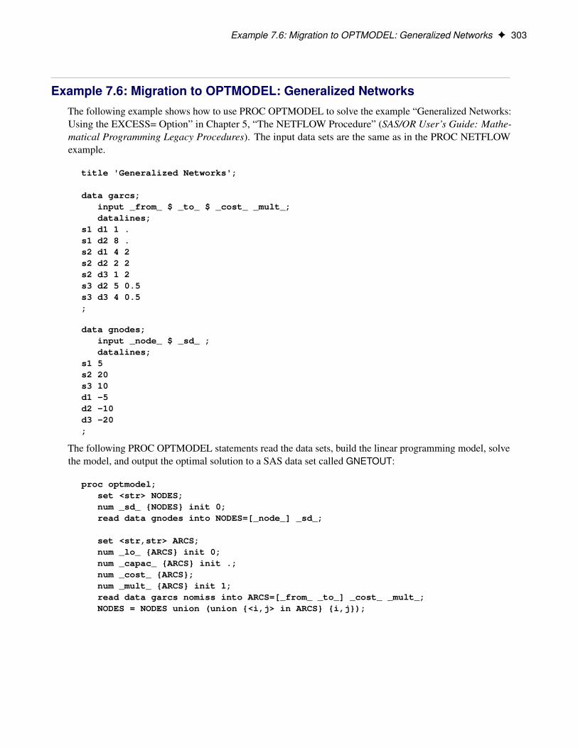
Example 7.6: Migration to OPTMODEL: Generalized Networks F 303
Example 7.6: Migration to OPTMODEL: Generalized NetworksThe following example shows how to use PROC OPTMODEL to solve the example “Generalized Networks:Using the EXCESS= Option” in Chapter 5, “The NETFLOW Procedure” (SAS/OR User’s Guide: Mathe-matical Programming Legacy Procedures). The input data sets are the same as in the PROC NETFLOWexample.
title 'Generalized Networks';
data garcs;input _from_ $ _to_ $ _cost_ _mult_;datalines;
s1 d1 1 .s1 d2 8 .s2 d1 4 2s2 d2 2 2s2 d3 1 2s3 d2 5 0.5s3 d3 4 0.5;
data gnodes;input _node_ $ _sd_ ;datalines;
s1 5s2 20s3 10d1 -5d2 -10d3 -20;
The following PROC OPTMODEL statements read the data sets, build the linear programming model, solvethe model, and output the optimal solution to a SAS data set called GNETOUT:
proc optmodel;set <str> NODES;num _sd_ {NODES} init 0;read data gnodes into NODES=[_node_] _sd_;
set <str,str> ARCS;num _lo_ {ARCS} init 0;num _capac_ {ARCS} init .;num _cost_ {ARCS};num _mult_ {ARCS} init 1;read data garcs nomiss into ARCS=[_from_ _to_] _cost_ _mult_;NODES = NODES union (union {<i,j> in ARCS} {i,j});
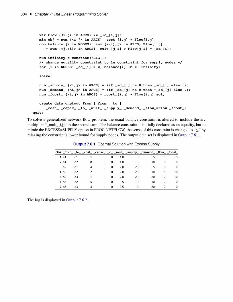
304 F Chapter 7: The Linear Programming Solver
var Flow {<i,j> in ARCS} >= _lo_[i,j];min obj = sum {<i,j> in ARCS} _cost_[i,j] * Flow[i,j];con balance {i in NODES}: sum {<(i),j> in ARCS} Flow[i,j]
- sum {<j,(i)> in ARCS} _mult_[j,i] * Flow[j,i] = _sd_[i];
num infinity = constant('BIG');/* change equality constraint to le constraint for supply nodes */for {i in NODES: _sd_[i] > 0} balance[i].lb = -infinity;
solve;
num _supply_ {<i,j> in ARCS} = (if _sd_[i] ne 0 then _sd_[i] else .);num _demand_ {<i,j> in ARCS} = (if _sd_[j] ne 0 then -_sd_[j] else .);num _fcost_ {<i,j> in ARCS} = _cost_[i,j] * Flow[i,j].sol;
create data gnetout from [_from_ _to_]_cost_ _capac_ _lo_ _mult_ _supply_ _demand_ _flow_=Flow _fcost_;
quit;
To solve a generalized network flow problem, the usual balance constraint is altered to include the arcmultiplier “_mult_[i,j]” in the second sum. The balance constraint is initially declared as an equality, but tomimic the EXCESS=SUPPLY option in PROC NETFLOW, the sense of this constraint is changed to “�” byrelaxing the constraint’s lower bound for supply nodes. The output data set is displayed in Output 7.6.1.
Output 7.6.1 Optimal Solution with Excess Supply
Obs _from_ _to_ _cost_ _capac_ _lo_ _mult_ _supply_ _demand_ _flow_ _fcost_
1 s1 d1 1 . 0 1.0 5 5 5 5
2 s1 d2 8 . 0 1.0 5 10 0 0
3 s2 d1 4 . 0 2.0 20 5 0 0
4 s2 d2 2 . 0 2.0 20 10 5 10
5 s2 d3 1 . 0 2.0 20 20 10 10
6 s3 d2 5 . 0 0.5 10 10 0 0
7 s3 d3 4 . 0 0.5 10 20 0 0
The log is displayed in Output 7.6.2.
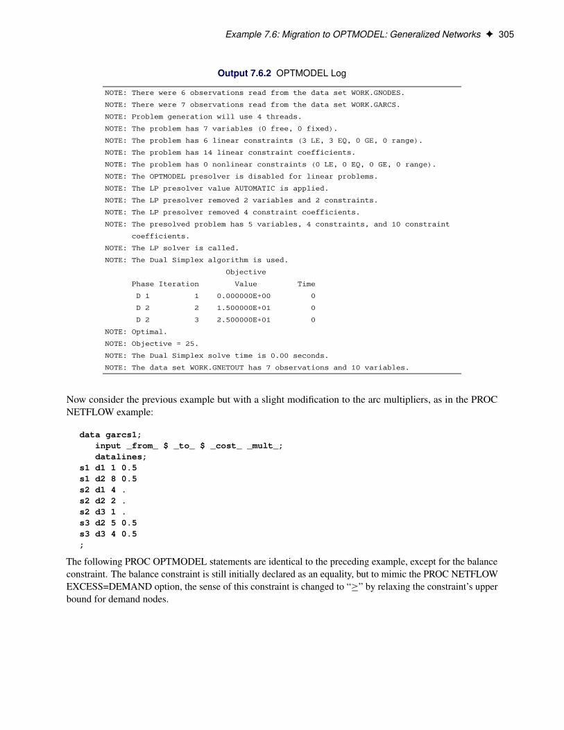
Example 7.6: Migration to OPTMODEL: Generalized Networks F 305
Output 7.6.2 OPTMODEL Log
NOTE: There were 6 observations read from the data set WORK.GNODES.
NOTE: There were 7 observations read from the data set WORK.GARCS.
NOTE: Problem generation will use 4 threads.
NOTE: The problem has 7 variables (0 free, 0 fixed).
NOTE: The problem has 6 linear constraints (3 LE, 3 EQ, 0 GE, 0 range).
NOTE: The problem has 14 linear constraint coefficients.
NOTE: The problem has 0 nonlinear constraints (0 LE, 0 EQ, 0 GE, 0 range).
NOTE: The OPTMODEL presolver is disabled for linear problems.
NOTE: The LP presolver value AUTOMATIC is applied.
NOTE: The LP presolver removed 2 variables and 2 constraints.
NOTE: The LP presolver removed 4 constraint coefficients.
NOTE: The presolved problem has 5 variables, 4 constraints, and 10 constraint
coefficients.
NOTE: The LP solver is called.
NOTE: The Dual Simplex algorithm is used.
Objective
Phase Iteration Value Time
D 1 1 0.000000E+00 0
D 2 2 1.500000E+01 0
D 2 3 2.500000E+01 0
NOTE: Optimal.
NOTE: Objective = 25.
NOTE: The Dual Simplex solve time is 0.00 seconds.
NOTE: The data set WORK.GNETOUT has 7 observations and 10 variables.
Now consider the previous example but with a slight modification to the arc multipliers, as in the PROCNETFLOW example:
data garcs1;input _from_ $ _to_ $ _cost_ _mult_;datalines;
s1 d1 1 0.5s1 d2 8 0.5s2 d1 4 .s2 d2 2 .s2 d3 1 .s3 d2 5 0.5s3 d3 4 0.5;
The following PROC OPTMODEL statements are identical to the preceding example, except for the balanceconstraint. The balance constraint is still initially declared as an equality, but to mimic the PROC NETFLOWEXCESS=DEMAND option, the sense of this constraint is changed to “�” by relaxing the constraint’s upperbound for demand nodes.
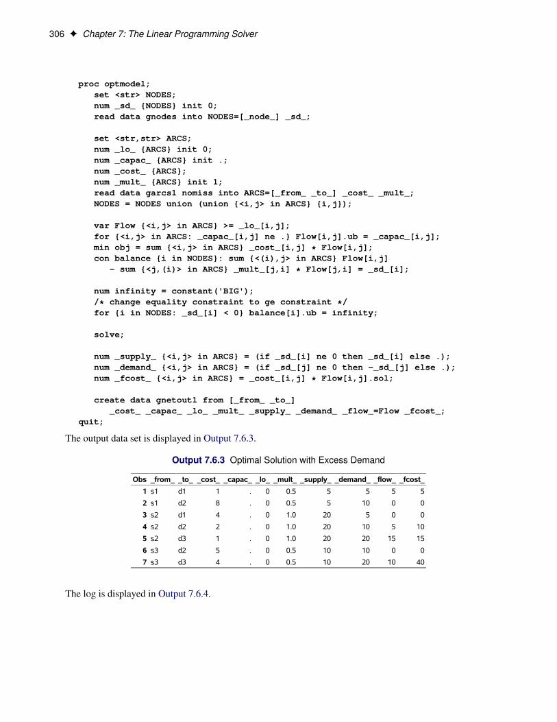
306 F Chapter 7: The Linear Programming Solver
proc optmodel;set <str> NODES;num _sd_ {NODES} init 0;read data gnodes into NODES=[_node_] _sd_;
set <str,str> ARCS;num _lo_ {ARCS} init 0;num _capac_ {ARCS} init .;num _cost_ {ARCS};num _mult_ {ARCS} init 1;read data garcs1 nomiss into ARCS=[_from_ _to_] _cost_ _mult_;NODES = NODES union (union {<i,j> in ARCS} {i,j});
var Flow {<i,j> in ARCS} >= _lo_[i,j];for {<i,j> in ARCS: _capac_[i,j] ne .} Flow[i,j].ub = _capac_[i,j];min obj = sum {<i,j> in ARCS} _cost_[i,j] * Flow[i,j];con balance {i in NODES}: sum {<(i),j> in ARCS} Flow[i,j]
- sum {<j,(i)> in ARCS} _mult_[j,i] * Flow[j,i] = _sd_[i];
num infinity = constant('BIG');/* change equality constraint to ge constraint */for {i in NODES: _sd_[i] < 0} balance[i].ub = infinity;
solve;
num _supply_ {<i,j> in ARCS} = (if _sd_[i] ne 0 then _sd_[i] else .);num _demand_ {<i,j> in ARCS} = (if _sd_[j] ne 0 then -_sd_[j] else .);num _fcost_ {<i,j> in ARCS} = _cost_[i,j] * Flow[i,j].sol;
create data gnetout1 from [_from_ _to_]_cost_ _capac_ _lo_ _mult_ _supply_ _demand_ _flow_=Flow _fcost_;
quit;
The output data set is displayed in Output 7.6.3.
Output 7.6.3 Optimal Solution with Excess Demand
Obs _from_ _to_ _cost_ _capac_ _lo_ _mult_ _supply_ _demand_ _flow_ _fcost_
1 s1 d1 1 . 0 0.5 5 5 5 5
2 s1 d2 8 . 0 0.5 5 10 0 0
3 s2 d1 4 . 0 1.0 20 5 0 0
4 s2 d2 2 . 0 1.0 20 10 5 10
5 s2 d3 1 . 0 1.0 20 20 15 15
6 s3 d2 5 . 0 0.5 10 10 0 0
7 s3 d3 4 . 0 0.5 10 20 10 40
The log is displayed in Output 7.6.4.
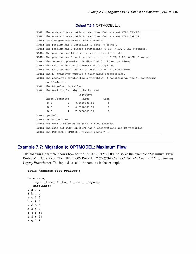
Example 7.7: Migration to OPTMODEL: Maximum Flow F 307
Output 7.6.4 OPTMODEL Log
NOTE: There were 6 observations read from the data set WORK.GNODES.
NOTE: There were 7 observations read from the data set WORK.GARCS1.
NOTE: Problem generation will use 4 threads.
NOTE: The problem has 7 variables (0 free, 0 fixed).
NOTE: The problem has 6 linear constraints (0 LE, 3 EQ, 3 GE, 0 range).
NOTE: The problem has 14 linear constraint coefficients.
NOTE: The problem has 0 nonlinear constraints (0 LE, 0 EQ, 0 GE, 0 range).
NOTE: The OPTMODEL presolver is disabled for linear problems.
NOTE: The LP presolver value AUTOMATIC is applied.
NOTE: The LP presolver removed 2 variables and 2 constraints.
NOTE: The LP presolver removed 4 constraint coefficients.
NOTE: The presolved problem has 5 variables, 4 constraints, and 10 constraint
coefficients.
NOTE: The LP solver is called.
NOTE: The Dual Simplex algorithm is used.
Objective
Phase Iteration Value Time
D 1 1 0.000000E+00 0
D 2 2 4.997000E+01 0
D 2 4 7.000000E+01 0
NOTE: Optimal.
NOTE: Objective = 70.
NOTE: The Dual Simplex solve time is 0.00 seconds.
NOTE: The data set WORK.GNETOUT1 has 7 observations and 10 variables.
NOTE: The PROCEDURE OPTMODEL printed pages 7-8.
Example 7.7: Migration to OPTMODEL: Maximum FlowThe following example shows how to use PROC OPTMODEL to solve the example “Maximum FlowProblem” in Chapter 5, “The NETFLOW Procedure” (SAS/OR User’s Guide: Mathematical ProgrammingLegacy Procedures). The input data set is the same as in that example.
title 'Maximum Flow Problem';
data arcs;input _from_ $ _to_ $ _cost_ _capac_;datalines;
S a . .S b . .a c 1 7b c 2 9a d 3 5b d 4 8c e 5 15d f 6 20e g 7 11
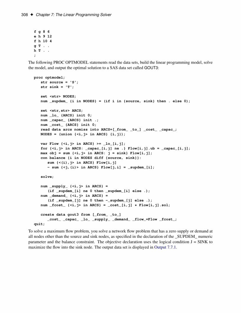
308 F Chapter 7: The Linear Programming Solver
f g 8 6e h 9 12f h 10 4g T . .h T . .;
The following PROC OPTMODEL statements read the data sets, build the linear programming model, solvethe model, and output the optimal solution to a SAS data set called GOUT3:
proc optmodel;str source = 'S';str sink = 'T';
set <str> NODES;num _supdem_ {i in NODES} = (if i in {source, sink} then . else 0);
set <str,str> ARCS;num _lo_ {ARCS} init 0;num _capac_ {ARCS} init .;num _cost_ {ARCS} init 0;read data arcs nomiss into ARCS=[_from_ _to_] _cost_ _capac_;NODES = (union {<i,j> in ARCS} {i,j});
var Flow {<i,j> in ARCS} >= _lo_[i,j];for {<i,j> in ARCS: _capac_[i,j] ne .} Flow[i,j].ub = _capac_[i,j];max obj = sum {<i,j> in ARCS: j = sink} Flow[i,j];con balance {i in NODES diff {source, sink}}:
sum {<(i),j> in ARCS} Flow[i,j]- sum {<j,(i)> in ARCS} Flow[j,i] = _supdem_[i];
solve;
num _supply_ {<i,j> in ARCS} =(if _supdem_[i] ne 0 then _supdem_[i] else .);
num _demand_ {<i,j> in ARCS} =(if _supdem_[j] ne 0 then -_supdem_[j] else .);
num _fcost_ {<i,j> in ARCS} = _cost_[i,j] * Flow[i,j].sol;
create data gout3 from [_from_ _to_]_cost_ _capac_ _lo_ _supply_ _demand_ _flow_=Flow _fcost_;
quit;
To solve a maximum flow problem, you solve a network flow problem that has a zero supply or demand atall nodes other than the source and sink nodes, as specified in the declaration of the _SUPDEM_ numericparameter and the balance constraint. The objective declaration uses the logical condition J = SINK tomaximize the flow into the sink node. The output data set is displayed in Output 7.7.1.
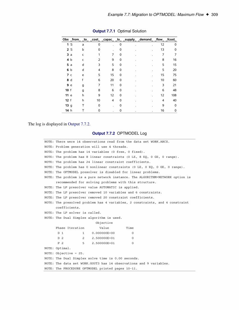
Example 7.7: Migration to OPTMODEL: Maximum Flow F 309
Output 7.7.1 Optimal Solution
Obs _from_ _to_ _cost_ _capac_ _lo_ _supply_ _demand_ _flow_ _fcost_
1 S a 0 . 0 . . 12 0
2 S b 0 . 0 . . 13 0
3 a c 1 7 0 . . 7 7
4 b c 2 9 0 . . 8 16
5 a d 3 5 0 . . 5 15
6 b d 4 8 0 . . 5 20
7 c e 5 15 0 . . 15 75
8 d f 6 20 0 . . 10 60
9 e g 7 11 0 . . 3 21
10 f g 8 6 0 . . 6 48
11 e h 9 12 0 . . 12 108
12 f h 10 4 0 . . 4 40
13 g T 0 . 0 . . 9 0
14 h T 0 . 0 . . 16 0
The log is displayed in Output 7.7.2.
Output 7.7.2 OPTMODEL Log
NOTE: There were 14 observations read from the data set WORK.ARCS.
NOTE: Problem generation will use 4 threads.
NOTE: The problem has 14 variables (0 free, 0 fixed).
NOTE: The problem has 8 linear constraints (0 LE, 8 EQ, 0 GE, 0 range).
NOTE: The problem has 24 linear constraint coefficients.
NOTE: The problem has 0 nonlinear constraints (0 LE, 0 EQ, 0 GE, 0 range).
NOTE: The OPTMODEL presolver is disabled for linear problems.
NOTE: The problem is a pure network instance. The ALGORITHM=NETWORK option is
recommended for solving problems with this structure.
NOTE: The LP presolver value AUTOMATIC is applied.
NOTE: The LP presolver removed 10 variables and 6 constraints.
NOTE: The LP presolver removed 20 constraint coefficients.
NOTE: The presolved problem has 4 variables, 2 constraints, and 4 constraint
coefficients.
NOTE: The LP solver is called.
NOTE: The Dual Simplex algorithm is used.
Objective
Phase Iteration Value Time
D 1 1 0.000000E+00 0
D 2 2 2.500000E+01 0
P 2 5 2.500000E+01 0
NOTE: Optimal.
NOTE: Objective = 25.
NOTE: The Dual Simplex solve time is 0.00 seconds.
NOTE: The data set WORK.GOUT3 has 14 observations and 9 variables.
NOTE: The PROCEDURE OPTMODEL printed pages 10-11.
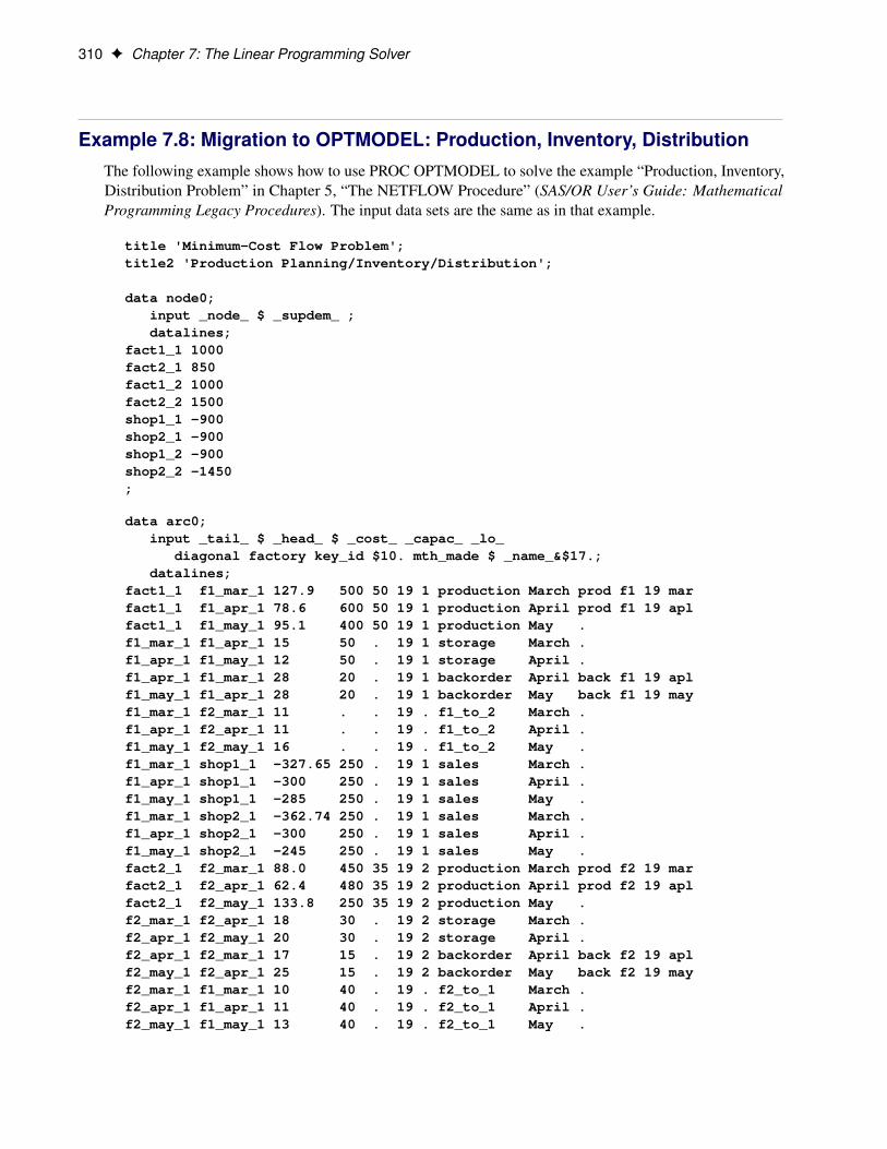
310 F Chapter 7: The Linear Programming Solver
Example 7.8: Migration to OPTMODEL: Production, Inventory, DistributionThe following example shows how to use PROC OPTMODEL to solve the example “Production, Inventory,Distribution Problem” in Chapter 5, “The NETFLOW Procedure” (SAS/OR User’s Guide: MathematicalProgramming Legacy Procedures). The input data sets are the same as in that example.
title 'Minimum-Cost Flow Problem';title2 'Production Planning/Inventory/Distribution';
data node0;input _node_ $ _supdem_ ;datalines;
fact1_1 1000fact2_1 850fact1_2 1000fact2_2 1500shop1_1 -900shop2_1 -900shop1_2 -900shop2_2 -1450;
data arc0;input _tail_ $ _head_ $ _cost_ _capac_ _lo_
diagonal factory key_id $10. mth_made $ _name_&$17.;datalines;
fact1_1 f1_mar_1 127.9 500 50 19 1 production March prod f1 19 marfact1_1 f1_apr_1 78.6 600 50 19 1 production April prod f1 19 aplfact1_1 f1_may_1 95.1 400 50 19 1 production May .f1_mar_1 f1_apr_1 15 50 . 19 1 storage March .f1_apr_1 f1_may_1 12 50 . 19 1 storage April .f1_apr_1 f1_mar_1 28 20 . 19 1 backorder April back f1 19 aplf1_may_1 f1_apr_1 28 20 . 19 1 backorder May back f1 19 mayf1_mar_1 f2_mar_1 11 . . 19 . f1_to_2 March .f1_apr_1 f2_apr_1 11 . . 19 . f1_to_2 April .f1_may_1 f2_may_1 16 . . 19 . f1_to_2 May .f1_mar_1 shop1_1 -327.65 250 . 19 1 sales March .f1_apr_1 shop1_1 -300 250 . 19 1 sales April .f1_may_1 shop1_1 -285 250 . 19 1 sales May .f1_mar_1 shop2_1 -362.74 250 . 19 1 sales March .f1_apr_1 shop2_1 -300 250 . 19 1 sales April .f1_may_1 shop2_1 -245 250 . 19 1 sales May .fact2_1 f2_mar_1 88.0 450 35 19 2 production March prod f2 19 marfact2_1 f2_apr_1 62.4 480 35 19 2 production April prod f2 19 aplfact2_1 f2_may_1 133.8 250 35 19 2 production May .f2_mar_1 f2_apr_1 18 30 . 19 2 storage March .f2_apr_1 f2_may_1 20 30 . 19 2 storage April .f2_apr_1 f2_mar_1 17 15 . 19 2 backorder April back f2 19 aplf2_may_1 f2_apr_1 25 15 . 19 2 backorder May back f2 19 mayf2_mar_1 f1_mar_1 10 40 . 19 . f2_to_1 March .f2_apr_1 f1_apr_1 11 40 . 19 . f2_to_1 April .f2_may_1 f1_may_1 13 40 . 19 . f2_to_1 May .
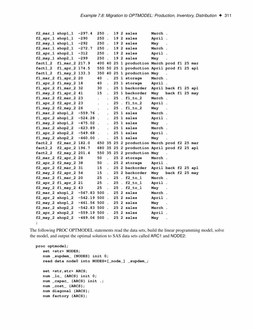
Example 7.8: Migration to OPTMODEL: Production, Inventory, Distribution F 311
f2_mar_1 shop1_1 -297.4 250 . 19 2 sales March .f2_apr_1 shop1_1 -290 250 . 19 2 sales April .f2_may_1 shop1_1 -292 250 . 19 2 sales May .f2_mar_1 shop2_1 -272.7 250 . 19 2 sales March .f2_apr_1 shop2_1 -312 250 . 19 2 sales April .f2_may_1 shop2_1 -299 250 . 19 2 sales May .fact1_2 f1_mar_2 217.9 400 40 25 1 production March prod f1 25 marfact1_2 f1_apr_2 174.5 550 50 25 1 production April prod f1 25 aplfact1_2 f1_may_2 133.3 350 40 25 1 production May .f1_mar_2 f1_apr_2 20 40 . 25 1 storage March .f1_apr_2 f1_may_2 18 40 . 25 1 storage April .f1_apr_2 f1_mar_2 32 30 . 25 1 backorder April back f1 25 aplf1_may_2 f1_apr_2 41 15 . 25 1 backorder May back f1 25 mayf1_mar_2 f2_mar_2 23 . . 25 . f1_to_2 March .f1_apr_2 f2_apr_2 23 . . 25 . f1_to_2 April .f1_may_2 f2_may_2 26 . . 25 . f1_to_2 May .f1_mar_2 shop1_2 -559.76 . . 25 1 sales March .f1_apr_2 shop1_2 -524.28 . . 25 1 sales April .f1_may_2 shop1_2 -475.02 . . 25 1 sales May .f1_mar_2 shop2_2 -623.89 . . 25 1 sales March .f1_apr_2 shop2_2 -549.68 . . 25 1 sales April .f1_may_2 shop2_2 -460.00 . . 25 1 sales May .fact2_2 f2_mar_2 182.0 650 35 25 2 production March prod f2 25 marfact2_2 f2_apr_2 196.7 680 35 25 2 production April prod f2 25 aplfact2_2 f2_may_2 201.4 550 35 25 2 production May .f2_mar_2 f2_apr_2 28 50 . 25 2 storage March .f2_apr_2 f2_may_2 38 50 . 25 2 storage April .f2_apr_2 f2_mar_2 31 15 . 25 2 backorder April back f2 25 aplf2_may_2 f2_apr_2 54 15 . 25 2 backorder May back f2 25 mayf2_mar_2 f1_mar_2 20 25 . 25 . f2_to_1 March .f2_apr_2 f1_apr_2 21 25 . 25 . f2_to_1 April .f2_may_2 f1_may_2 43 25 . 25 . f2_to_1 May .f2_mar_2 shop1_2 -567.83 500 . 25 2 sales March .f2_apr_2 shop1_2 -542.19 500 . 25 2 sales April .f2_may_2 shop1_2 -461.56 500 . 25 2 sales May .f2_mar_2 shop2_2 -542.83 500 . 25 2 sales March .f2_apr_2 shop2_2 -559.19 500 . 25 2 sales April .f2_may_2 shop2_2 -489.06 500 . 25 2 sales May .;
The following PROC OPTMODEL statements read the data sets, build the linear programming model, solvethe model, and output the optimal solution to SAS data sets called ARC1 and NODE2:
proc optmodel;set <str> NODES;num _supdem_ {NODES} init 0;read data node0 into NODES=[_node_] _supdem_;
set <str,str> ARCS;num _lo_ {ARCS} init 0;num _capac_ {ARCS} init .;num _cost_ {ARCS};num diagonal {ARCS};num factory {ARCS};
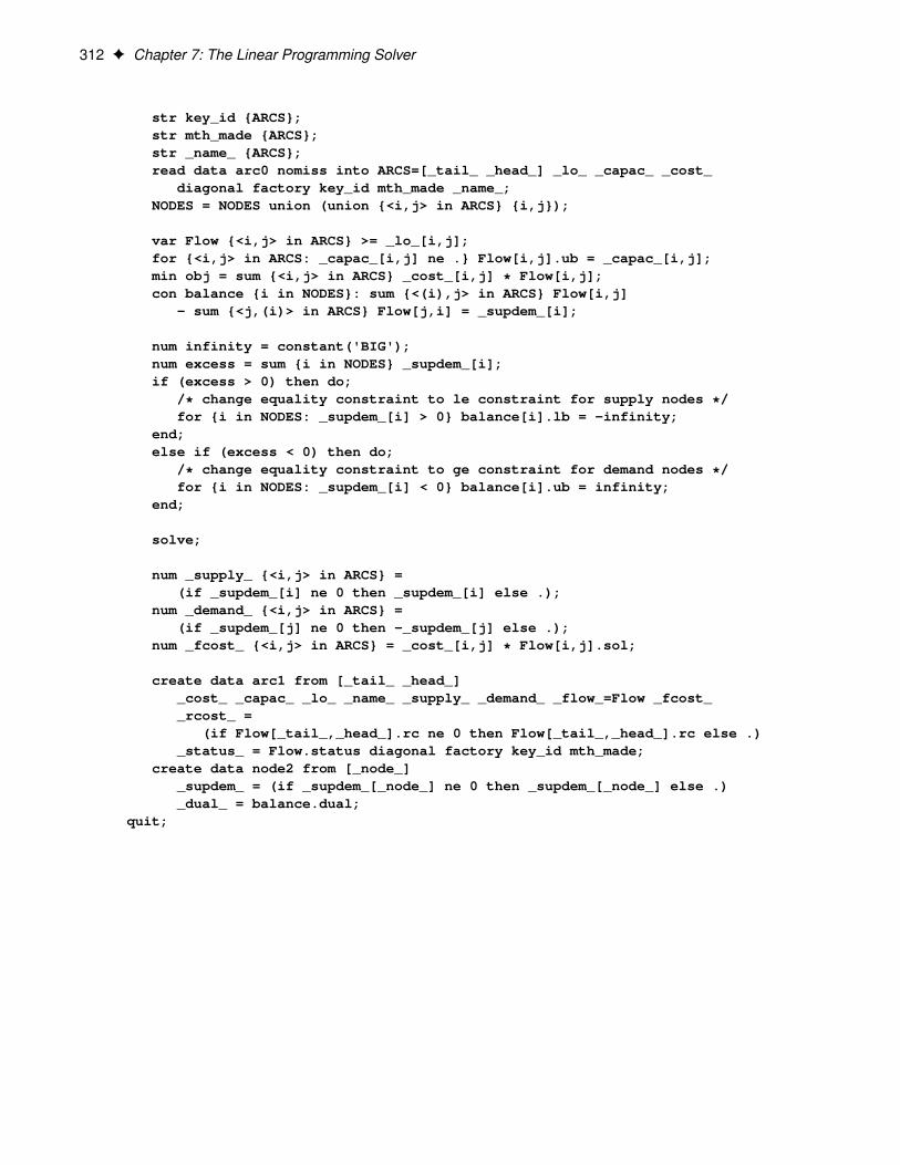
312 F Chapter 7: The Linear Programming Solver
str key_id {ARCS};str mth_made {ARCS};str _name_ {ARCS};read data arc0 nomiss into ARCS=[_tail_ _head_] _lo_ _capac_ _cost_
diagonal factory key_id mth_made _name_;NODES = NODES union (union {<i,j> in ARCS} {i,j});
var Flow {<i,j> in ARCS} >= _lo_[i,j];for {<i,j> in ARCS: _capac_[i,j] ne .} Flow[i,j].ub = _capac_[i,j];min obj = sum {<i,j> in ARCS} _cost_[i,j] * Flow[i,j];con balance {i in NODES}: sum {<(i),j> in ARCS} Flow[i,j]
- sum {<j,(i)> in ARCS} Flow[j,i] = _supdem_[i];
num infinity = constant('BIG');num excess = sum {i in NODES} _supdem_[i];if (excess > 0) then do;
/* change equality constraint to le constraint for supply nodes */for {i in NODES: _supdem_[i] > 0} balance[i].lb = -infinity;
end;else if (excess < 0) then do;
/* change equality constraint to ge constraint for demand nodes */for {i in NODES: _supdem_[i] < 0} balance[i].ub = infinity;
end;
solve;
num _supply_ {<i,j> in ARCS} =(if _supdem_[i] ne 0 then _supdem_[i] else .);
num _demand_ {<i,j> in ARCS} =(if _supdem_[j] ne 0 then -_supdem_[j] else .);
num _fcost_ {<i,j> in ARCS} = _cost_[i,j] * Flow[i,j].sol;
create data arc1 from [_tail_ _head_]_cost_ _capac_ _lo_ _name_ _supply_ _demand_ _flow_=Flow _fcost__rcost_ =
(if Flow[_tail_,_head_].rc ne 0 then Flow[_tail_,_head_].rc else .)_status_ = Flow.status diagonal factory key_id mth_made;
create data node2 from [_node_]_supdem_ = (if _supdem_[_node_] ne 0 then _supdem_[_node_] else .)_dual_ = balance.dual;
quit;
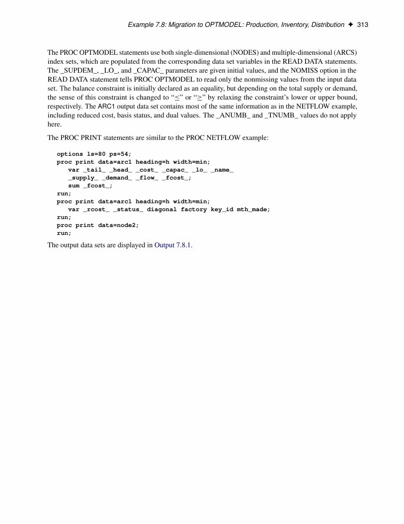
Example 7.8: Migration to OPTMODEL: Production, Inventory, Distribution F 313
The PROC OPTMODEL statements use both single-dimensional (NODES) and multiple-dimensional (ARCS)index sets, which are populated from the corresponding data set variables in the READ DATA statements.The _SUPDEM_, _LO_, and _CAPAC_ parameters are given initial values, and the NOMISS option in theREAD DATA statement tells PROC OPTMODEL to read only the nonmissing values from the input dataset. The balance constraint is initially declared as an equality, but depending on the total supply or demand,the sense of this constraint is changed to “�” or “�” by relaxing the constraint’s lower or upper bound,respectively. The ARC1 output data set contains most of the same information as in the NETFLOW example,including reduced cost, basis status, and dual values. The _ANUMB_ and _TNUMB_ values do not applyhere.
The PROC PRINT statements are similar to the PROC NETFLOW example:
options ls=80 ps=54;proc print data=arc1 heading=h width=min;
var _tail_ _head_ _cost_ _capac_ _lo_ _name__supply_ _demand_ _flow_ _fcost_;sum _fcost_;
run;proc print data=arc1 heading=h width=min;
var _rcost_ _status_ diagonal factory key_id mth_made;run;proc print data=node2;run;
The output data sets are displayed in Output 7.8.1.
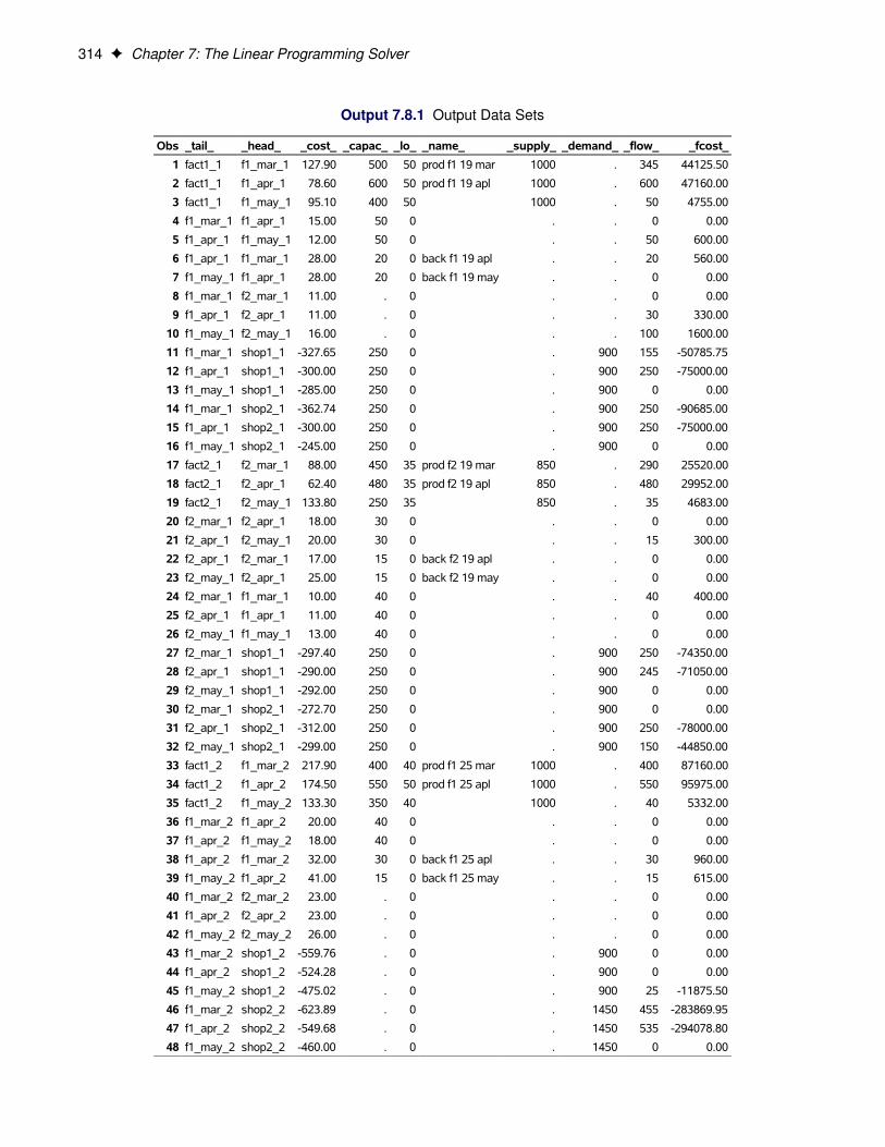
314 F Chapter 7: The Linear Programming Solver
Output 7.8.1 Output Data Sets
Obs _tail_ _head_ _cost_ _capac_ _lo_ _name_ _supply_ _demand_ _flow_ _fcost_
1 fact1_1 f1_mar_1 127.90 500 50 prod f1 19 mar 1000 . 345 44125.50
2 fact1_1 f1_apr_1 78.60 600 50 prod f1 19 apl 1000 . 600 47160.00
3 fact1_1 f1_may_1 95.10 400 50 1000 . 50 4755.00
4 f1_mar_1 f1_apr_1 15.00 50 0 . . 0 0.00
5 f1_apr_1 f1_may_1 12.00 50 0 . . 50 600.00
6 f1_apr_1 f1_mar_1 28.00 20 0 back f1 19 apl . . 20 560.00
7 f1_may_1 f1_apr_1 28.00 20 0 back f1 19 may . . 0 0.00
8 f1_mar_1 f2_mar_1 11.00 . 0 . . 0 0.00
9 f1_apr_1 f2_apr_1 11.00 . 0 . . 30 330.00
10 f1_may_1 f2_may_1 16.00 . 0 . . 100 1600.00
11 f1_mar_1 shop1_1 -327.65 250 0 . 900 155 -50785.75
12 f1_apr_1 shop1_1 -300.00 250 0 . 900 250 -75000.00
13 f1_may_1 shop1_1 -285.00 250 0 . 900 0 0.00
14 f1_mar_1 shop2_1 -362.74 250 0 . 900 250 -90685.00
15 f1_apr_1 shop2_1 -300.00 250 0 . 900 250 -75000.00
16 f1_may_1 shop2_1 -245.00 250 0 . 900 0 0.00
17 fact2_1 f2_mar_1 88.00 450 35 prod f2 19 mar 850 . 290 25520.00
18 fact2_1 f2_apr_1 62.40 480 35 prod f2 19 apl 850 . 480 29952.00
19 fact2_1 f2_may_1 133.80 250 35 850 . 35 4683.00
20 f2_mar_1 f2_apr_1 18.00 30 0 . . 0 0.00
21 f2_apr_1 f2_may_1 20.00 30 0 . . 15 300.00
22 f2_apr_1 f2_mar_1 17.00 15 0 back f2 19 apl . . 0 0.00
23 f2_may_1 f2_apr_1 25.00 15 0 back f2 19 may . . 0 0.00
24 f2_mar_1 f1_mar_1 10.00 40 0 . . 40 400.00
25 f2_apr_1 f1_apr_1 11.00 40 0 . . 0 0.00
26 f2_may_1 f1_may_1 13.00 40 0 . . 0 0.00
27 f2_mar_1 shop1_1 -297.40 250 0 . 900 250 -74350.00
28 f2_apr_1 shop1_1 -290.00 250 0 . 900 245 -71050.00
29 f2_may_1 shop1_1 -292.00 250 0 . 900 0 0.00
30 f2_mar_1 shop2_1 -272.70 250 0 . 900 0 0.00
31 f2_apr_1 shop2_1 -312.00 250 0 . 900 250 -78000.00
32 f2_may_1 shop2_1 -299.00 250 0 . 900 150 -44850.00
33 fact1_2 f1_mar_2 217.90 400 40 prod f1 25 mar 1000 . 400 87160.00
34 fact1_2 f1_apr_2 174.50 550 50 prod f1 25 apl 1000 . 550 95975.00
35 fact1_2 f1_may_2 133.30 350 40 1000 . 40 5332.00
36 f1_mar_2 f1_apr_2 20.00 40 0 . . 0 0.00
37 f1_apr_2 f1_may_2 18.00 40 0 . . 0 0.00
38 f1_apr_2 f1_mar_2 32.00 30 0 back f1 25 apl . . 30 960.00
39 f1_may_2 f1_apr_2 41.00 15 0 back f1 25 may . . 15 615.00
40 f1_mar_2 f2_mar_2 23.00 . 0 . . 0 0.00
41 f1_apr_2 f2_apr_2 23.00 . 0 . . 0 0.00
42 f1_may_2 f2_may_2 26.00 . 0 . . 0 0.00
43 f1_mar_2 shop1_2 -559.76 . 0 . 900 0 0.00
44 f1_apr_2 shop1_2 -524.28 . 0 . 900 0 0.00
45 f1_may_2 shop1_2 -475.02 . 0 . 900 25 -11875.50
46 f1_mar_2 shop2_2 -623.89 . 0 . 1450 455 -283869.95
47 f1_apr_2 shop2_2 -549.68 . 0 . 1450 535 -294078.80
48 f1_may_2 shop2_2 -460.00 . 0 . 1450 0 0.00
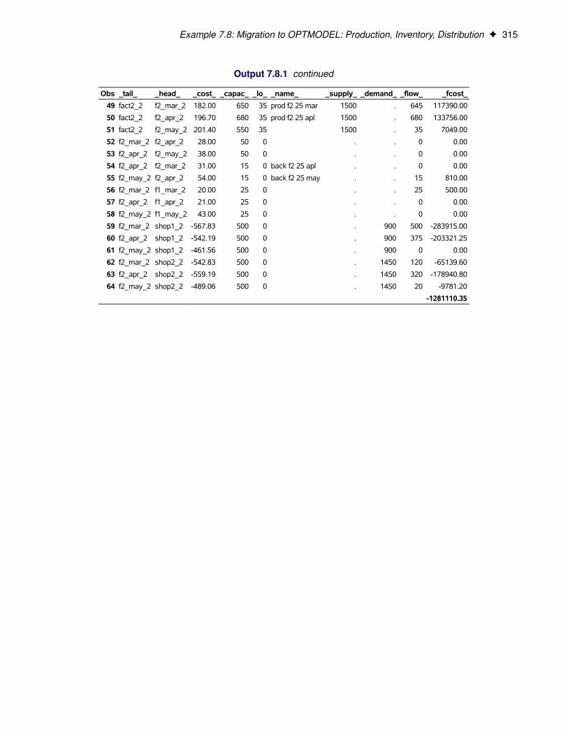
Example 7.8: Migration to OPTMODEL: Production, Inventory, Distribution F 315
Output 7.8.1 continued
Obs _tail_ _head_ _cost_ _capac_ _lo_ _name_ _supply_ _demand_ _flow_ _fcost_
49 fact2_2 f2_mar_2 182.00 650 35 prod f2 25 mar 1500 . 645 117390.00
50 fact2_2 f2_apr_2 196.70 680 35 prod f2 25 apl 1500 . 680 133756.00
51 fact2_2 f2_may_2 201.40 550 35 1500 . 35 7049.00
52 f2_mar_2 f2_apr_2 28.00 50 0 . . 0 0.00
53 f2_apr_2 f2_may_2 38.00 50 0 . . 0 0.00
54 f2_apr_2 f2_mar_2 31.00 15 0 back f2 25 apl . . 0 0.00
55 f2_may_2 f2_apr_2 54.00 15 0 back f2 25 may . . 15 810.00
56 f2_mar_2 f1_mar_2 20.00 25 0 . . 25 500.00
57 f2_apr_2 f1_apr_2 21.00 25 0 . . 0 0.00
58 f2_may_2 f1_may_2 43.00 25 0 . . 0 0.00
59 f2_mar_2 shop1_2 -567.83 500 0 . 900 500 -283915.00
60 f2_apr_2 shop1_2 -542.19 500 0 . 900 375 -203321.25
61 f2_may_2 shop1_2 -461.56 500 0 . 900 0 0.00
62 f2_mar_2 shop2_2 -542.83 500 0 . 1450 120 -65139.60
63 f2_apr_2 shop2_2 -559.19 500 0 . 1450 320 -178940.80
64 f2_may_2 shop2_2 -489.06 500 0 . 1450 20 -9781.20
-1281110.35
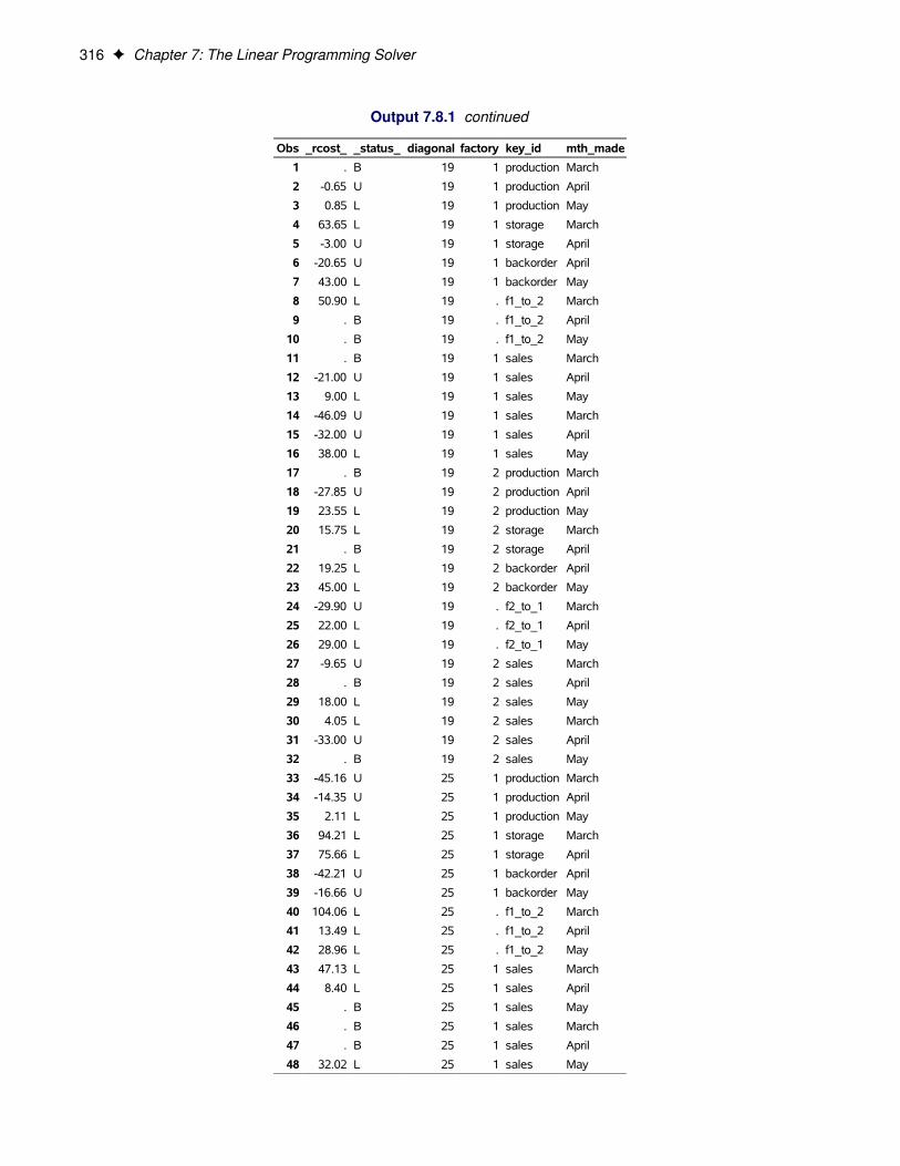
316 F Chapter 7: The Linear Programming Solver
Output 7.8.1 continued
Obs _rcost_ _status_ diagonal factory key_id mth_made
1 . B 19 1 production March
2 -0.65 U 19 1 production April
3 0.85 L 19 1 production May
4 63.65 L 19 1 storage March
5 -3.00 U 19 1 storage April
6 -20.65 U 19 1 backorder April
7 43.00 L 19 1 backorder May
8 50.90 L 19 . f1_to_2 March
9 . B 19 . f1_to_2 April
10 . B 19 . f1_to_2 May
11 . B 19 1 sales March
12 -21.00 U 19 1 sales April
13 9.00 L 19 1 sales May
14 -46.09 U 19 1 sales March
15 -32.00 U 19 1 sales April
16 38.00 L 19 1 sales May
17 . B 19 2 production March
18 -27.85 U 19 2 production April
19 23.55 L 19 2 production May
20 15.75 L 19 2 storage March
21 . B 19 2 storage April
22 19.25 L 19 2 backorder April
23 45.00 L 19 2 backorder May
24 -29.90 U 19 . f2_to_1 March
25 22.00 L 19 . f2_to_1 April
26 29.00 L 19 . f2_to_1 May
27 -9.65 U 19 2 sales March
28 . B 19 2 sales April
29 18.00 L 19 2 sales May
30 4.05 L 19 2 sales March
31 -33.00 U 19 2 sales April
32 . B 19 2 sales May
33 -45.16 U 25 1 production March
34 -14.35 U 25 1 production April
35 2.11 L 25 1 production May
36 94.21 L 25 1 storage March
37 75.66 L 25 1 storage April
38 -42.21 U 25 1 backorder April
39 -16.66 U 25 1 backorder May
40 104.06 L 25 . f1_to_2 March
41 13.49 L 25 . f1_to_2 April
42 28.96 L 25 . f1_to_2 May
43 47.13 L 25 1 sales March
44 8.40 L 25 1 sales April
45 . B 25 1 sales May
46 . B 25 1 sales March
47 . B 25 1 sales April
48 32.02 L 25 1 sales May
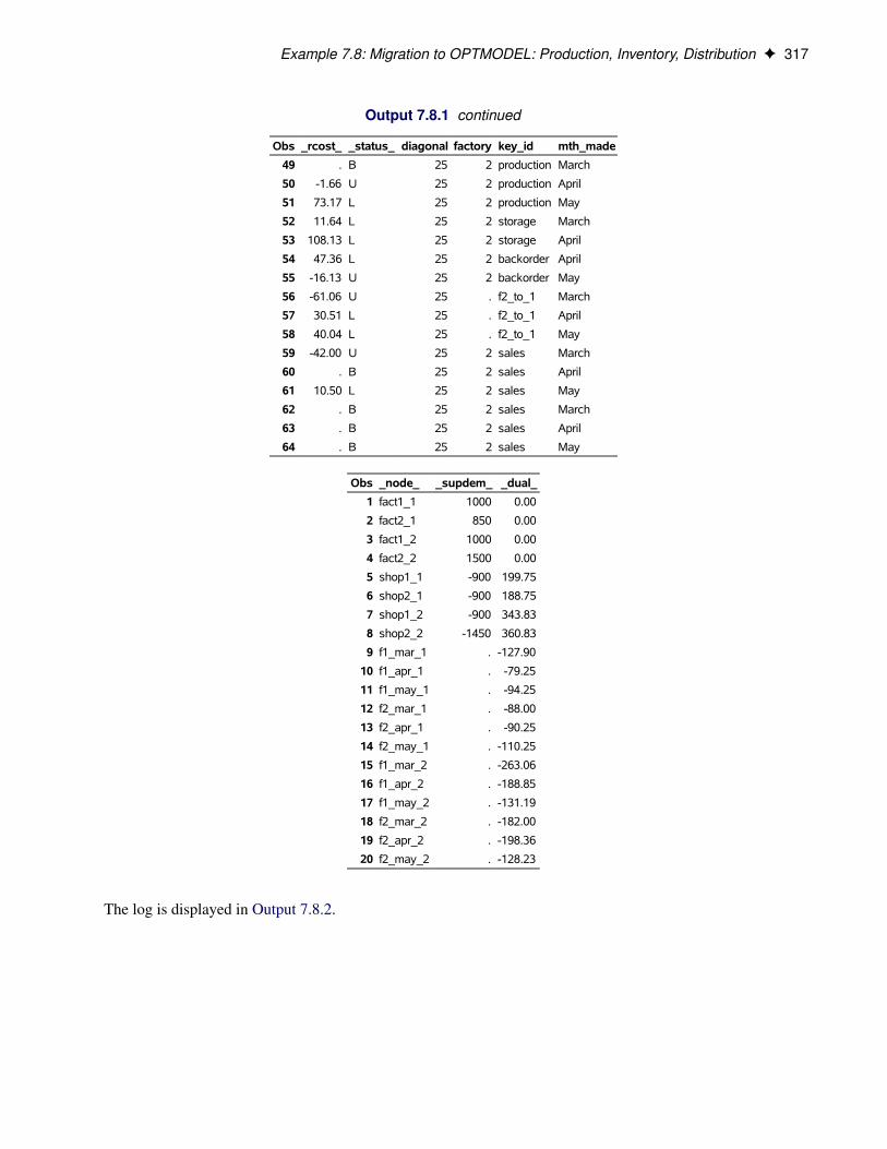
Example 7.8: Migration to OPTMODEL: Production, Inventory, Distribution F 317
Output 7.8.1 continued
Obs _rcost_ _status_ diagonal factory key_id mth_made
49 . B 25 2 production March
50 -1.66 U 25 2 production April
51 73.17 L 25 2 production May
52 11.64 L 25 2 storage March
53 108.13 L 25 2 storage April
54 47.36 L 25 2 backorder April
55 -16.13 U 25 2 backorder May
56 -61.06 U 25 . f2_to_1 March
57 30.51 L 25 . f2_to_1 April
58 40.04 L 25 . f2_to_1 May
59 -42.00 U 25 2 sales March
60 . B 25 2 sales April
61 10.50 L 25 2 sales May
62 . B 25 2 sales March
63 . B 25 2 sales April
64 . B 25 2 sales May
Obs _node_ _supdem_ _dual_
1 fact1_1 1000 0.00
2 fact2_1 850 0.00
3 fact1_2 1000 0.00
4 fact2_2 1500 0.00
5 shop1_1 -900 199.75
6 shop2_1 -900 188.75
7 shop1_2 -900 343.83
8 shop2_2 -1450 360.83
9 f1_mar_1 . -127.90
10 f1_apr_1 . -79.25
11 f1_may_1 . -94.25
12 f2_mar_1 . -88.00
13 f2_apr_1 . -90.25
14 f2_may_1 . -110.25
15 f1_mar_2 . -263.06
16 f1_apr_2 . -188.85
17 f1_may_2 . -131.19
18 f2_mar_2 . -182.00
19 f2_apr_2 . -198.36
20 f2_may_2 . -128.23
The log is displayed in Output 7.8.2.
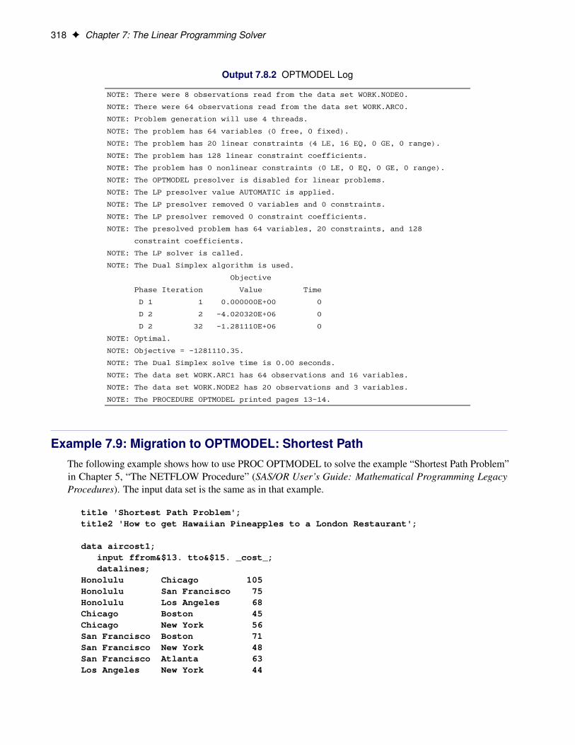
318 F Chapter 7: The Linear Programming Solver
Output 7.8.2 OPTMODEL Log
NOTE: There were 8 observations read from the data set WORK.NODE0.
NOTE: There were 64 observations read from the data set WORK.ARC0.
NOTE: Problem generation will use 4 threads.
NOTE: The problem has 64 variables (0 free, 0 fixed).
NOTE: The problem has 20 linear constraints (4 LE, 16 EQ, 0 GE, 0 range).
NOTE: The problem has 128 linear constraint coefficients.
NOTE: The problem has 0 nonlinear constraints (0 LE, 0 EQ, 0 GE, 0 range).
NOTE: The OPTMODEL presolver is disabled for linear problems.
NOTE: The LP presolver value AUTOMATIC is applied.
NOTE: The LP presolver removed 0 variables and 0 constraints.
NOTE: The LP presolver removed 0 constraint coefficients.
NOTE: The presolved problem has 64 variables, 20 constraints, and 128
constraint coefficients.
NOTE: The LP solver is called.
NOTE: The Dual Simplex algorithm is used.
Objective
Phase Iteration Value Time
D 1 1 0.000000E+00 0
D 2 2 -4.020320E+06 0
D 2 32 -1.281110E+06 0
NOTE: Optimal.
NOTE: Objective = -1281110.35.
NOTE: The Dual Simplex solve time is 0.00 seconds.
NOTE: The data set WORK.ARC1 has 64 observations and 16 variables.
NOTE: The data set WORK.NODE2 has 20 observations and 3 variables.
NOTE: The PROCEDURE OPTMODEL printed pages 13-14.
Example 7.9: Migration to OPTMODEL: Shortest PathThe following example shows how to use PROC OPTMODEL to solve the example “Shortest Path Problem”in Chapter 5, “The NETFLOW Procedure” (SAS/OR User’s Guide: Mathematical Programming LegacyProcedures). The input data set is the same as in that example.
title 'Shortest Path Problem';title2 'How to get Hawaiian Pineapples to a London Restaurant';
data aircost1;input ffrom&$13. tto&$15. _cost_;datalines;
Honolulu Chicago 105Honolulu San Francisco 75Honolulu Los Angeles 68Chicago Boston 45Chicago New York 56San Francisco Boston 71San Francisco New York 48San Francisco Atlanta 63Los Angeles New York 44
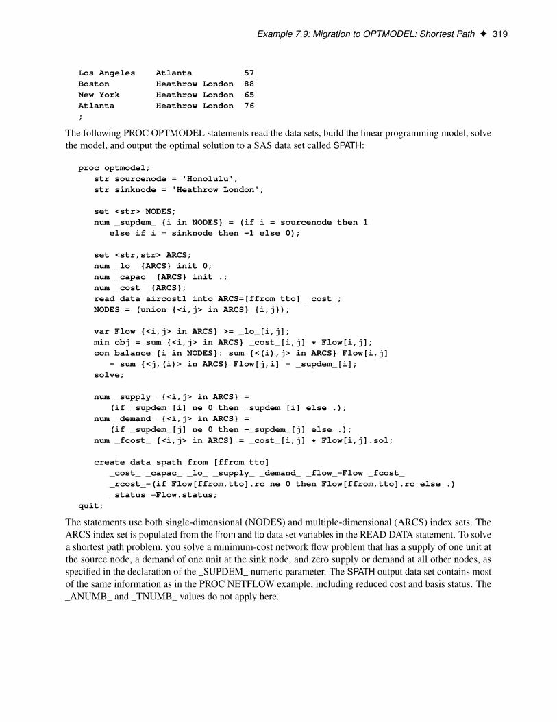
Example 7.9: Migration to OPTMODEL: Shortest Path F 319
Los Angeles Atlanta 57Boston Heathrow London 88New York Heathrow London 65Atlanta Heathrow London 76;
The following PROC OPTMODEL statements read the data sets, build the linear programming model, solvethe model, and output the optimal solution to a SAS data set called SPATH:
proc optmodel;str sourcenode = 'Honolulu';str sinknode = 'Heathrow London';
set <str> NODES;num _supdem_ {i in NODES} = (if i = sourcenode then 1
else if i = sinknode then -1 else 0);
set <str,str> ARCS;num _lo_ {ARCS} init 0;num _capac_ {ARCS} init .;num _cost_ {ARCS};read data aircost1 into ARCS=[ffrom tto] _cost_;NODES = (union {<i,j> in ARCS} {i,j});
var Flow {<i,j> in ARCS} >= _lo_[i,j];min obj = sum {<i,j> in ARCS} _cost_[i,j] * Flow[i,j];con balance {i in NODES}: sum {<(i),j> in ARCS} Flow[i,j]
- sum {<j,(i)> in ARCS} Flow[j,i] = _supdem_[i];solve;
num _supply_ {<i,j> in ARCS} =(if _supdem_[i] ne 0 then _supdem_[i] else .);
num _demand_ {<i,j> in ARCS} =(if _supdem_[j] ne 0 then -_supdem_[j] else .);
num _fcost_ {<i,j> in ARCS} = _cost_[i,j] * Flow[i,j].sol;
create data spath from [ffrom tto]_cost_ _capac_ _lo_ _supply_ _demand_ _flow_=Flow _fcost__rcost_=(if Flow[ffrom,tto].rc ne 0 then Flow[ffrom,tto].rc else .)_status_=Flow.status;
quit;
The statements use both single-dimensional (NODES) and multiple-dimensional (ARCS) index sets. TheARCS index set is populated from the ffrom and tto data set variables in the READ DATA statement. To solvea shortest path problem, you solve a minimum-cost network flow problem that has a supply of one unit atthe source node, a demand of one unit at the sink node, and zero supply or demand at all other nodes, asspecified in the declaration of the _SUPDEM_ numeric parameter. The SPATH output data set contains mostof the same information as in the PROC NETFLOW example, including reduced cost and basis status. The_ANUMB_ and _TNUMB_ values do not apply here.
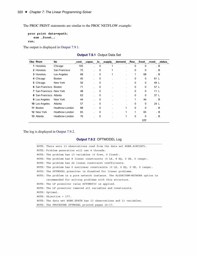
320 F Chapter 7: The Linear Programming Solver
The PROC PRINT statements are similar to the PROC NETFLOW example:
proc print data=spath;sum _fcost_;
run;
The output is displayed in Output 7.9.1.
Output 7.9.1 Output Data Set
Obs ffrom tto _cost_ _capac_ _lo_ _supply_ _demand_ _flow_ _fcost_ _rcost_ _status_
1 Honolulu Chicago 105 . 0 1 . 0 0 . B
2 Honolulu San Francisco 75 . 0 1 . 0 0 . B
3 Honolulu Los Angeles 68 . 0 1 . 1 68 . B
4 Chicago Boston 45 . 0 . . 0 0 61 L
5 Chicago New York 56 . 0 . . 0 0 49 L
6 San Francisco Boston 71 . 0 . . 0 0 57 L
7 San Francisco New York 48 . 0 . . 0 0 11 L
8 San Francisco Atlanta 63 . 0 . . 0 0 37 L
9 Los Angeles New York 44 . 0 . . 1 44 . B
10 Los Angeles Atlanta 57 . 0 . . 0 0 24 L
11 Boston Heathrow London 88 . 0 . 1 0 0 . B
12 New York Heathrow London 65 . 0 . 1 1 65 . B
13 Atlanta Heathrow London 76 . 0 . 1 0 0 . B
177
The log is displayed in Output 7.9.2.
Output 7.9.2 OPTMODEL Log
NOTE: There were 13 observations read from the data set WORK.AIRCOST1.
NOTE: Problem generation will use 4 threads.
NOTE: The problem has 13 variables (0 free, 0 fixed).
NOTE: The problem has 8 linear constraints (0 LE, 8 EQ, 0 GE, 0 range).
NOTE: The problem has 26 linear constraint coefficients.
NOTE: The problem has 0 nonlinear constraints (0 LE, 0 EQ, 0 GE, 0 range).
NOTE: The OPTMODEL presolver is disabled for linear problems.
NOTE: The problem is a pure network instance. The ALGORITHM=NETWORK option is
recommended for solving problems with this structure.
NOTE: The LP presolver value AUTOMATIC is applied.
NOTE: The LP presolver removed all variables and constraints.
NOTE: Optimal.
NOTE: Objective = 177.
NOTE: The data set WORK.SPATH has 13 observations and 11 variables.
NOTE: The PROCEDURE OPTMODEL printed pages 16-17.
References F 321
References
Ahuja, R. K., Magnanti, T. L., and Orlin, J. B. (1993). Network Flows: Theory, Algorithms, and Applications.Englewood Cliffs, NJ: Prentice-Hall.
Andersen, E. D., and Andersen, K. D. (1995). “Presolving in Linear Programming.” MathematicalProgramming 71:221–245.
Dantzig, G. B. (1963). Linear Programming and Extensions. Princeton, NJ: Princeton University Press.
Forrest, J. J., and Goldfarb, D. (1992). “Steepest-Edge Simplex Algorithms for Linear Programming.”Mathematical Programming 5:1–28.
Gondzio, J. (1997). “Presolve Analysis of Linear Programs Prior to Applying an Interior Point Method.”INFORMS Journal on Computing 9:73–91.
Harris, P. M. J. (1973). “Pivot Selection Methods in the Devex LP Code.” Mathematical Programming57:341–374.
Maros, I. (2003). Computational Techniques of the Simplex Method. Boston: Kluwer Academic.
Subject Index
algorithm, 260
basis, 264
concurrent LP, 272constraint status
LP solver, 273
decomposition algorithmLP solver, 265
dualization, 261
feasibility tolerance, 262
IIS optionOPTMODEL procedure, LP solver, 274
irreducible infeasible setOPTMODEL procedure, LP solver, 274
iteration logcrossover algorithm, 271interior point algorithm, 271LP solver, 269–271network simplex algorithm, 270primal and dual simplex algorithms, 269
linear programming, see also OPTMODEL procedureLP solver
concurrent LP, 272constraint status, 273iteration log, 269–271problem statistics, 272variable status, 273
LP solver examplesdiet problem, 278finding an irreducible infeasible set, 292generalized networks, 303maximum flow, 307production, inventory, distribution, 310shortest path, 318two-person zero-sum game, 289using the network simplex algorithm, 295
macro variable_OROPTMODEL_, 275
migration to PROC OPTMODELfrom PROC NETFLOW, 303, 307, 310, 318
OPTMODEL proceduredualization, 261
OPTMODEL procedure, LP solver
algorithm2, 261basis, 264feasibility tolerance, 262functional summary, 259IIS option, 274introductory example, 256macro variable _OROPTMODEL_, 275network simplex algorithm, 266preprocessing, 261presolver, 261pricing, 264queue size, 264scaling, 264solver, 260
_OROPTMODEL_ macro variable, 275
presolver, 261pricing, 264
queue size, 264
random seed, 265
scaling, 264SOLVE WITH LP statement
crossover, 265dual infeasibility, 265duality gap, 265primal infeasibility, 265
variable statusLP solver, 273

Syntax Index
ALGORITHM2= optionSOLVE WITH LP statement, 261
ALGORITHM= optionSOLVE WITH LP statement, 260
BASIS= optionSOLVE WITH LP statement, 264
CROSSOVER= optionSOLVE WITH LP statement, 265
DECOMP_MASTER=() optionSOLVE WITH LP statement, 265
DECOMP=() optionSOLVE WITH LP statement, 265
DECOMP_SUBPROB=() optionSOLVE WITH LP statement, 266
DUALIZE= optionSOLVE WITH LP statement, 261
FEASTOL= optionSOLVE WITH LP statement, 262
IIS= optionSOLVE WITH LP statement, 260
LOGFREQ= optionSOLVE WITH LP statement, 262
LOGLEVEL= optionSOLVE WITH LP statement, 262
MAXITER= optionSOLVE WITH LP statement, 262
MAXTIME= optionSOLVE WITH LP statement, 263
OPTMODEL procedure, LP solversyntax, 259
OPTTOL= optionSOLVE WITH LP statement, 263
PRESOLVER= optionSOLVE WITH LP statement, 261
PRICETYPE= optionSOLVE WITH LP statement, 264
PRINTFREQ= optionSOLVE WITH LP statement, 262
PRINTLEVEL2= optionSOLVE WITH LP statement, 262
QUEUESIZE= optionSOLVE WITH LP statement, 264
SCALE= optionSOLVE WITH LP statement, 264
SEED= optionSOLVE WITH LP statement, 265
SOL= optionSOLVE WITH LP statement, 260
SOLVE WITH LP statementALGORITHM2= option, 261ALGORITHM= option, 260BASIS= option, 264CROSSOVER= option, 265DECOMP_MASTER=() option, 265DECOMP=() option, 265DECOMP_SUBPROB=() option, 266DUALIZE= option, 261FEASTOL= option, 262IIS= option, 260LOGFREQ= option, 262LOGLEVEL= option, 262MAXITER= option, 262MAXTIME= option, 263OPTTOL= option, 263PRESOLVER= option, 261PRICETYPE= option, 264PRINTFREQ= option, 262PRINTLEVEL2= option, 262QUEUESIZE= option, 264SCALE= option, 264SEED= option, 265SOL= option, 260SOLVER2= option, 261SOLVER= option, 260STOP_DG= option, 265STOP_DI= option, 265STOP_PI= option, 265TIMETYPE= option, 263
SOLVER2= optionSOLVE WITH LP statement, 261
SOLVER= optionSOLVE WITH LP statement, 260
STOP_DG= optionSOLVE WITH LP statement, 265
STOP_DI= optionSOLVE WITH LP statement, 265
STOP_PI= option

SOLVE WITH LP statement, 265
TIMETYPE= optionSOLVE WITH LP statement, 263


