The Loss of Confidence on Bank Money in the Great Depression By Andrea Gerali and Franco Passacantando 1 1. Introduction ................................................................................................................................. 2 2. Some evidence on the impact of bank failures on bank money .................................................. 2 3. The role of transaction services in the demand for money ......................................................... 5 4. Difference with other approaches ............................................................................................... 7 5. Measuring the impact of bank failures on the use of bank payment instruments ..................... 11 6. The impact on output of the fall of confidence in bank money ................................................ 17 7. Conclusion ................................................................................................................................ 19 1 This paper has had a long gestation, as it was first drafted in 1993 while the authors were at the University of Berkeley, respectively as graduate student and visiting scholar. Helpful comments have been provided, at various stages, by Paolo Angelini, Ben Bernanke, Curzio Giannini, Berry Eichengreen. We thank Gerardo Palazzo for the support provided in data elaboration. Of course the responsibility for the results presented is entirely ours.
Transcript
The Loss of Confidence on Bank Money in the Great Depression
1 This paper has had a long gestation, as it was first drafted in 1993 while the authors were at the University of Berkeley, respectively as graduate student and visiting scholar. Helpful comments have been provided, at various stages, by Paolo Angelini, Ben Bernanke, Curzio Giannini, Berry Eichengreen. We thank Gerardo Palazzo for the support provided in data elaboration. Of course the responsibility for the results presented is entirely ours.
2
1. Introduction
During the Great Depression the level of prices declined, hence the real value of the
existing stock of money increased, and yet its use as a payment medium plunged. We argue
that the fall in the use of money was at least to some extent unrelated to the pattern of money
creation, and instead also the consequence of a drastic deterioration in the acceptance of bank
money as payment medium. Bank money, being a credit instrument, bears a credit risk which
normally is negligible but in rare circumstances it sharply increases to the point of triggering
a generalized confidence crisis, in its use as a payment instrument, with significant
macroeconimic consequences.
The thesis we present has different policy implications from the one implicit in the
traditional monetarist view of the Great Depression. A more expansionary monetary policy,
even if it had succeeded in increasing the stock of money in circulation, would not have
affected the willingness of the public to use it as an exchange medium. Seemingly, also a
more expansionary fiscal policy could have had limited effect on the constraint to spending
represented by the mistrust on a valid payment medium. The problems of confidence we
highlight can be addressed only by structural measures in the area of banking. And indeed it is
only with the introduction of federal insurance of bank deposits in 1933 and the strengthening
of emergency lending powers of the Federal Reserve Banks, together with closer regulation of
banks that the confidence in bank money was restored. These measures, together with the
suspension of the gold standard eventually led to the resumption of growth after 1933.
The rest of the paper is organized as follows. The next section presents some data and
facts which show the extent of the loss of confidence on bank money and its relation with the
waves of bank failures between [October] 1930 and March 1933. Section 3 further spells out
the hypothesis of the paper while section 4 highlights the difference with other thesis on the
effect of bank failures on the Great Depression. Section 5 presents and discusses the
econometric evidence in support of the argument that bank failures triggered a confidence
crisis in bank money. Section 6 presents some, mainly anecdotal, evidence on how this had an
impact on consumption and output and section 7 concludes.
2. Some evidence on the impact of bank failures on bank money
3
The loss of confidence in bankmoney was related to the chain of bank failures that took
place in the period between [October] 1930 and March 1933. In the last two months of 1930,
608 banks failed, including the Bank of the United States which was the largest bank ever
failed in the US.3 Bank suspensions dramatically increased thereafter and in the four years
until 1933, more than 9000 banks suspended their operations, representing more than one fifth
of the commercial banks in the United States.4 The impact on the use of bank money was
amplified by the fact that often bank suspensions were accompanied by restrictions on cash
withdrawals imposed either by the banks or by local, state and federal authorities.
A vivid picture of the impact of all this on the economy is in the words of many
commentators of the times, who single out the loss of confidence within the business sector as
the most important reason for the depression:
“This factor of confidence is an intangible one and greatly underestimated. Gradually we have developed to a point where 90 per cent of our transactions are conducted on credit…….[and] only one out of ten of our daily business transactions is a cash transaction. The nine others depend upon our state of mind. If doubt enters and one out of the nine deals falls through, there is a slowdown of ten per cent, and much less than a 10 per cent slowdown changes the nation’s figures from black to red”.5
Bank failures not only determined a sharp reduction in the stock of bank deposits
available but also affected the payment habits and the whole payment technology that was
used at the time. Looking at the statistics on bank deposits published by the Fed, the use of
checks, the most common instrument to mobilize bank money for payment purposes, fell
sharply in those years. From a peak of 367 billion dollars in 1929 the value of all the checks
handled by the Federal Reserve Banks fell to 158 billion dollars in 1933. The drop is much
greater than the 49 per cent fall in nominal income that occurred in those years, as shown in
3 The Bank bore a name that “led many at home and abroad to regard it somehow as an official bank”, Friedman and Schwartz , op.cit. pp 310 311.
4 Federal Reserve Bulletin, September 1937, page 907 and Friedman & Schwartz op.cit. p. 299.
5 Merle Thorpe ”Cheerful Facts about 1930” World’s Work, May 1931.
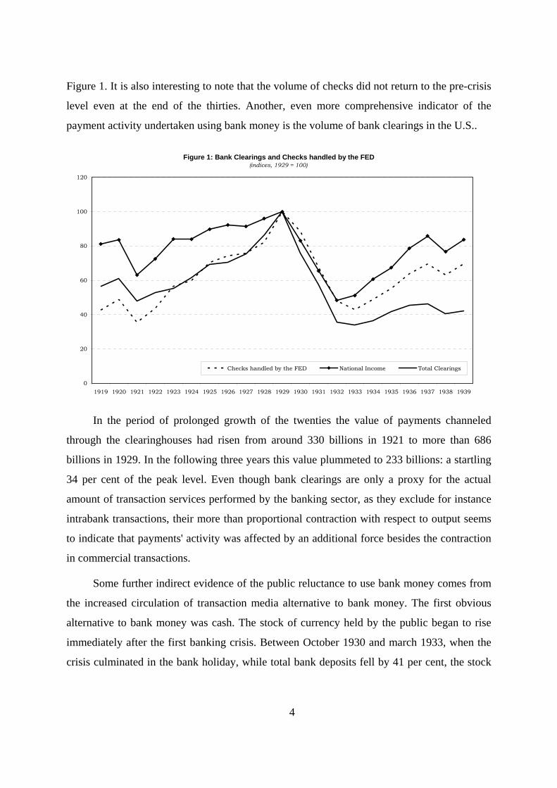
Figure 1. It is also interesting to note that the volume of checks did not return to the pre-crisis
level even at the end of the thirties. Another, even more comprehensive indicator of the
payment activity undertaken using bank money is the volume of bank clearings in the U.S..
Figure 1: Bank Clearings and Checks handled by the FED(indices, 1929 = 100)
Checks handled by the FED National Income Total Clearings
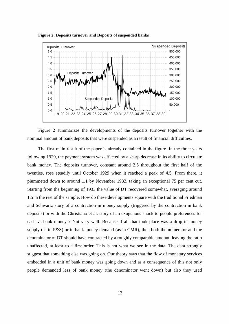
In the period of prolonged growth of the twenties the value of payments channeled
through the clearinghouses had risen from around 330 billions in 1921 to more than 686
billions in 1929. In the following three years this value plummeted to 233 billions: a startling
34 per cent of the peak level. Even though bank clearings are only a proxy for the actual
amount of transaction services performed by the banking sector, as they exclude for instance
intrabank transactions, their more than proportional contraction with respect to output seems
to indicate that payments' activity was affected by an additional force besides the contraction
in commercial transactions.
Some further indirect evidence of the public reluctance to use bank money comes from
the increased circulation of transaction media alternative to bank money. The first obvious
alternative to bank money was cash. The stock of currency held by the public began to rise
immediately after the first banking crisis. Between October 1930 and march 1933, when the
crisis culminated in the bank holiday, while total bank deposits fell by 41 per cent, the stock
4
5
of currency increased by 53 per cent.6 However the increase in currency did not offset the fall
in the deposits and the sum of the two aggregates fell by 33 per cent. Cash is in fact a poor
substitute of bank money, especially for large value or interregional transactions. Postal
savings also behaved in a fashion very similar to that of currency but they suffered the
limitation that no checks could be written against them. Another sign of the growing concerns
for using bank money was the shift of deposits, especially those held by large corporate
customers, into regions of the country such as New York or Philadelphia, where they were
perceived as safer.7
Finally, many rural and urban communities within the United States introduced various
forms of barter, often associated with new instruments such as scrip or stamped money.8 Also
trade acceptances came into existence precisely in this period as an attempt to conduct
business without relying on a network of interbank credit relationships. As will be further
discussed in Section 6 almost all these media were either more expensive or less practical
than traditional forms of bank money. The willingness to face these extra costs is de facto
evidence of the deep distrust in bank money. It however implied that additional resources
costs had to be paid, thus subtracting from the efficiency of the economy.
3. The role of transaction services in the demand for money
The facts presented in the previous section are well known. However traditionally they
have been considered only insofar as they affected the portfolio adjustments between bank
deposits, currency, and bonds, and hence primarily the level of interest rates. We instead
focus on the nature of the relationship between real money balances and the flow of
transaction services generated by it and argue that the increase in credit risk associated with
the use of bank money generated a structural break in such a relationship.
6 These data are drawn by Friedman and Schwartz , op cit. Appendix A.
7 See Angell (1936) as referred to by Rockoff (1993) pp.9-10.
8 The main center for the organized barter movement was Los Angeles County, California. The scrip was issued in the form of booklets containing certificates of various denominations used to exchange goods within community associations. Sometimes only stamped scripts were accepted, with the stamps usually issued by local authorities.
6
This risk has various components. A first type of risk, the debtor risk, is related to the
probability of insolvency of the debtor, for instance the issuer of a check in a payment.
Another risk, the settlement risk is related to the probability of default of the bank where the
deposits are held or of possible restrictions of withdrawals from those deposits. Finally there
is what nowadays is called the systemic risk, i.e. . the risk related to the possibility that the
bank of the debtor will be unable to complete the transfer of funds because of the failure of
some other bank involved in the chain of payment transfers. Systemic risk is particularly
problematic for two reasons. First, it cannot be assessed by simply considering the financial
soundness and overall performance of the buyer's bank. The probability of failure during the
settlement lag depends on the probability of intervening failures of other financial institutions
that can, via the complex web of interbank transactions, trigger a chain reaction of successive
insolvencies that may ultimately affect even a financially solid institution.10 Second, this risk
is positively correlated with the length of the settlement lag, i.e. with the time lag between
completion of the exchange of the payment instrument (say a check) and the settlement of the
underlying transaction, since the chances of an intervening failure by some other agent are
greater as time elapses. This risk therefore tends to be greater for checks of small banks and
for those of banks located in distant areas.
As with any form of credit risk, the way to hedge against it would be to properly
diversify the instruments bearing that risk. Furthermore, the proper allocation of risks would
require its proper pricing. Neither condition holds for the specific risks we are dealing with.
First of all, diversification of deposits is costly and impractical, especially for small deposit
holders. Secondly, information asymmetries complicate the assessment of the default risk of a
bank, especially for small deposit holders. Thirdly, the settlement risk cannot be easily
assessed in advance, nor transferred or pooled or hedged against. Since it has to be borne
entirely by the individual, it greatly increases the costs associated with the use of bank
money.
10 The most important contribution to the definition of systemic risk and to its measurement in present day in payment systems is that of Humphrey (1986).
7
Given the difficulties to properly assess risks ex ante, when one such risk materializes
agents switch out of bank deposits and, as this process gets momentum, the value of bank
money as a medium of exchange is reduced for everybody, because of network externalities.
The more people start refusing my checks as a valid form of payment the less my bank
account is valued to me, because the flow of transaction services embedded in it has
deteriorated as a result of its reduced degree of acceptability.
If the substitutes of bank money were to offer the same transaction services associated
with bank money, and if the acceptability of these instruments were the same as that for bank
money, the impact of all this on the economy would be negligible. However, if this is not true,
as we will argue, the impact on the economy can be significant. The substitution of a system
based on bank money with an alternative one is a lengthy process and may ultimately imply
greater costs. The system based on checks relies on cooperative arrangements, usually
centered around clearinghouses, on information and transportation networks, and on legal
provisions that are not easily transferable to alternative systems. In the short run the search for
an alternative system certainly implies additional costs. Furthermore, instruments different
from checks, such as letters of credits, drafts or commercial papers, imply greater information
costs because they rely on bilateral credit assessment and may give rise to liquidity
constraints. These constraints may negatively affect in particular financial transactions, for
which speed of execution is crucial.
It is thus highly likely that spending decisions of economic agents are negatively
affected by the increase in costs brought about by the deterioration of the quality of the
transaction services associated with a given stock of money in the economy, i.e., in the degree
of "moneyness" of that stock of money. And it is also equally likely that this has a
contractionary effect on aggregate output distinct from the ones working through the
monetary supply and the credit and intermediation services. The impact of the deterioration of
the services provided by money on output may be similar to that produced by a sudden
change in the cost of energy or by a major collapse of the transportation system,
independently form the portfolio adjustment it generates.
4. Difference with other approaches
8
In focusing on the relationship between money balances and the flows of transaction
services generated by it we reach conclusions about the role of money supply in the Great
Depression which complement those of the monetarist (i.e. Friedman and Schwartz) and the
Keynesian (i.e. Temin, Eichengreen etc.) side of the debate.
Notoriously, Friedman and Schwartz (F&S thereafter), in their 1963 work, argue that
the contraction of money supply was the main cause of the crisis. They believe that bank
failures had two consequences on income: a wealth effect on consumption, stemming from
the capital losses suffered by shareholders and depositors of the failed banks, and an effect on
aggregate demand due to the drastic decline in the stock of money, given the policy followed
by the Reserve System. The authors show that, of the two effects, the latter was by far the
most important in negatively affecting the real economy. The contraction of money supply
resulted from the freezing of bank deposits in closed banks and from the withdrawal of
deposits by panicked depositors who feared bank failure. The refusal on the part of a growing
number of banks to honor their commitment to exchange deposits for currency at par
produced a devaluation of deposits against currency. The policy followed by the Fed, which
did not offset the contraction of the supply of bank with monetary base creation, amplified the
recession.
Their view of the role of bank crisiss is somehwhat paradoxical. For example, F&S
assert that "The bank failures were important not primarily in their own right, but because of
their indirect effect. If they had occurred to precisely the same extent without producing a
drastic decline in the stock of money, they would have been notable but not crucial. If they
had not occurred but a correspondingly sharp decline had been produced in the stock of
money by some other means, the contraction would have been at least equally severe and
probably even more so".11 And the contraction would have been stronger because for them
bank failures, by reducing the attractiveness of bank deposits, had a positive impact on
income velocity, in the sense that they limited the decline in income velocity that took place.
So for them “the bank failures, by their effect on the demand for money, offset some of the
harm they did by their effect on the supply of money”. According to our view instead, even if
the stock of money had been higher, for instance through a less restrictive policy by the Fed, a
9
contractionary effect would have occurred anyway, since the acceptability of bank money had
deteriorated and the transaction services associated with it would have decreased. Conversely,
if no bank failures had occurred, the contraction of bank money would have been associated
with a smaller deterioration in its degree of "moneyness" and the contractionary effect would
have been less pronounced. An opposite conclusion from that of F&S.
In their monetary history, F&S do not explicitly mention the channels through which
money affects the economy.12 Variations of the money stock have an effect on the economy
either because changes in the volume of one financial asset affect the prices of other assets or
through interest rate movements. The volume of transaction services associated with the use
of money is considered as a constant or as a variable moving along a trend. This hypothesis is
clearly invalid in a period such the Great Depression, in which the ability of banks to provide
payment services was affected by the crisis.
In a 1993 paper, Hugh Rockoff addresses this issue and shows how a decline in what he
calls “the quality of the money stock” contributed to the severity of the contraction. By
redefining the stock of money to take into account that part of the available money could not
be used for transactions, he finds a stronger relationship between money and output.
However, for Rockoff, the deterioration in the quality of money has an impact on income
because “a decrease in quality would lead to an attempt to build up total liquid balances,
putting downward pressure on spending”13. He does not inquire into how the deterioration of
moneyness affects both the substitutes of money and the bank deposits at surviving banks
(which he still treat as money), and therefore concentrates on a portfolio effect, only applied
to money stocks that are adjusted to take into account the degree of moneyness.
To a certain extent our approach is closer to that of Bernanke (1983), even though he
focuses on credit rather than on monetary aspects. He argues that the monetarist view cannot
11 Friedman and Schwartz (1963), p. 352.
12 In the demand for money developed in Friedman (1956) "dollars of money are not distinguished according as they are said to be held for one or the other purpose" (p.14). His demand for money does not contain as an explanatory variable the volume of transactions but the "more basic technical and cost conditions that affect the costs of conserving money" (p.12).
13 Rockoff (1993), p. 10.
10
be a satisfactory explanation because "… no theory of monetary effects on the real economy
can explain protracted non neutrality" (p. 257). He also claims that bank failures did produce
non-monetary consequences because they increased the cost of the credit intermediation
services traditionally performed by banks. Once he found an empirical relationship between
bank failures and the cost of credit intermediation, he can easily infer an impact on real
income through a combination of two effects, one on aggregate supply, due to the difficulties
in funding worthwhile activities and investments and the consequent diversion in the
allocation of available funds to inferior uses; and the other on aggregate demand, due to the
substitution of present for future consumption given the relative higher cost of financing
consumption today. Banks suffer losses coming from asset depreciations and contraction in
deposits, as depositors reacted to widespread bank weaknesses by withdrawing their funds.
The consequent rise in cost of credit intermediation forced even borrowers with viable
projects and strong balance sheets to experience a contraction in the availability of loans. In
concentrating on credit intermediation, Bernanke acknowledges that he is neglecting "the
transactions and other services performed by banks" (p. 263, nt.18). His analysis therefore
assumes either that there were no changes in the availability of banks' transaction services or,
most likely, that these changes had a negligible impact on the economy.
Our approach is perhaps closest in spirit to the original work of Klein (1974) and to
some recent extensions of it contained in Giannini (2004). Klein builds a theory of competing
monies centered around the concept that each type of money produces a different amount of
monetary services depending on the amount of “confidence” in its future value that users
attach to that variety. Giannini, building on this approach, explains the evolution and
circulation of different kind of moneys in different historical periods as optimal responses to
the problem of producing such “confidence” in the future value of money. In his model, the
flows of services generated by money are a function of three factors: the quantity of money
held, the level of prices, and a confidence factor, measuring how confident people are about
the ability of money to preserve its future exchange value (since the utility of money depends
on the possibility to spend it, and thus on the rate of exchange between money and real
goods). Compared to these approaches, we share the idea that money is worth only insofar as
it provides monetary services and that, to produce such services, money needs to enjoy some
degree of “confidence” from the part of its final users, but we relate the confidence factor not
11
only to the risk of depreciation of the underlying asset, but also to the risk of default of the
issuer.
Our theory can also complement a recent work by Christiano, Motto and Rostagno
(2004) on the causes and forces behind the Great Depression. Their analysis is based on a
dynamic stochastic general equilibrium model where some of the equations describing agents’
behavior are subject to (unexplained) stochastic disturbances. According to the model
solution and the authors’ calibration of the parameters, one element turns out to be at the heart
of the contraction phase of the depression. In their words, the trigger of the depression was
“… a liquidity preference shock […] that drove households to accumulate currency at the
expense of demand deposits and other [bank] liabilities, like time deposits" (p. 3). Therefore,
using a sophisticated methodology, these authors come to the conclusion that “something”
happened during the first phase of the depression that induced households to shift away from
bank money and into currency (or other substitutes of it). Being a stochastic shock in their
model, their analysis is silent about the fundamental origins of this “something” and they can
only conjecture that perhaps this shock “…might not be invariant to the nature of monetary
policy”. Our analysis attaches a name to the culprit, arguing that the fundamental “shock” was
the wave of bank failures and the observed shift from bank money into currency was only a
consequence of the resulting reduction in transaction services (via the “loss of confidence”
effect).
5. Measuring the impact of bank failures on the use of bank payment instruments
In this section we present empirical results (based on our monthly data set of
observations for the US; see the Data Appendix) to evaluate the empirical relevance of the
“loss of confidence” effect in the demand for bank money. We want to test the hypothesis that
the large number of bank defaults increased the credit risk associated with the use of bank
money and reduced the demand of bank money for transaction purposes. To put it differently,
the hypothesis is that, for any given level of income, bank money was used less than would
have been otherwise because it contained less transaction services built into it.
A key step in this exercise is finding a good proxy measure for the transaction services
performed by bank money. A natural candidate to look at are the bank clearings data we
presented in the introduction. This variable measures the total amount of financial
12
transactions performed using bank money in a given period. But for our analysis in the
following we decided to focus on bank debits instead. These are defined as the sum of all the
transactions that affect bank deposit accounts, including those finalized between two clients
of the same bank.
There are several reasons to prefer this measure over bank clearings. For one reason,
bank clearings may overstate the extent of the fall in the use of bank money, since they are
affected by the sharp reduction in the number of banks in operation that occurred in that
period. This effect would bias the results in our favor and thus we decided to use a measure
that was not subject to this spurious correlation. Moreover, bank clearings focus on only a
subset of bank money, since they record only financial transactions that needed to be cleared
with a transfer of funds from one bank to another, and do not contain transactions among
clients of the same bank. Again, excluding same-bank transactions would have probably
biased the results in our favor, i.e. increased the positive correlation between bank failures
and banking transactions (because the increased settlement risk induced by bank failures
matters only for transactions among clients of different banks). Finally, banks debts data
come at monthly frequency and have a broader geographical coverage.
For all these reasons, the variable used as proxy of the transaction services embedded in
bank money is the “Turnover of Deposits” (DT thereafter), defined as the ratio of bank debits
to bank deposits. This ratio records at its numerator the flow of all transactions that impinged
on bank deposit accounts, and normalize them by the total of bank deposits (excluding those
of failed banks, of course) out of which that flow was produced. Again, the variable attempts
to measure the “pace” at which the “payment system” associated to bank money was
operating at any moment in time, and can thus be considered a proxy of its efficiency.
Figure 2: Deposits turnover and Deposits of suspended banks
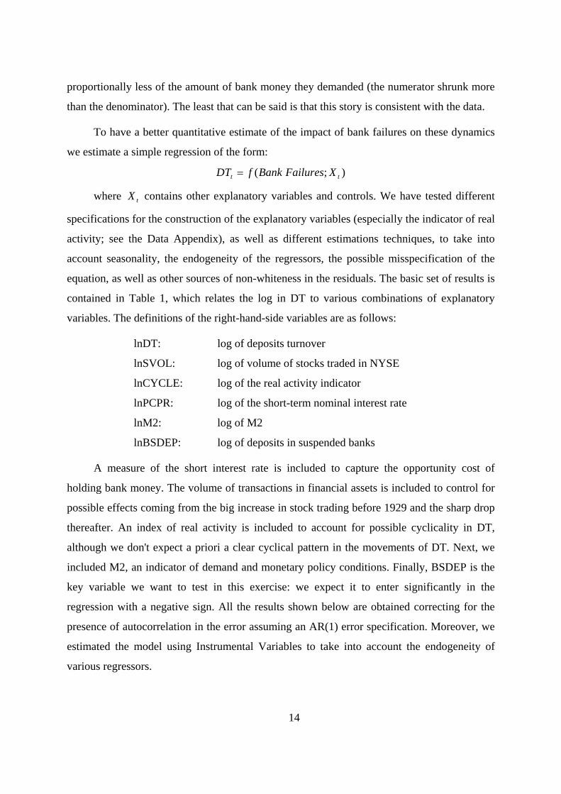
Impact from a 100% increase in BSDEP - -7.49% -7.37% -6.59% -4.78%
(4) (5)
Notes: Bold numbers indicate a coefficient significant at the 95% confidence level. An asterisk indicates significanceabove the 99% threshold. In all the equations, we instrument lnSVOL, lnCYCLE, lnPCPR and lnM2 using theirlagged values.
Table 1: Regressions on Log of Deposits Turnover (lnDT)
(1) (2) (3)
We started with a simple regression relating DT to traditional regressors without any
variable directly related to the banking crisis. Results are shown as eq. (1) in Table 1. The
equation seems to provide a decent fit but the coefficients turn out to be rather sensible to the
inclusion/exclusion of specific regressors (a clear sign of misspecification). We next added
our proposed regressor BSDEP, and since we suspect that the loss of confidence induced by
the waves of bank failures was a gradual and incremental phenomenon, we includes up to 4
lagged values of BSDEP. As can be seen from eqs. (2), (3) and (4), whenever these variables
are added to the regression they enter with the right sign and strongly significantly (except for
the fourth lag, which is never significant although it always has the right sign); overall, they
tend to stabilize other regressors’ coefficients and to improve the regression fit, with a R2
going from 0.55 up to 0.77.
We also tried other specifications for the DT equation (including lagged values of the
other regressors, or changing the error specification) and in all attempts the coefficients
15
16
attached to the BSDEP variables turn out to be remarkably stable. Eq. (5) reports one such
attempt (we chose to report this one because, among the specifications tried, it is a lower
bound in term of significance of our BSDEP variables) in which we included the lagged
endogenous variable among the regressors. As can be seen from the table, there is an obvious
improvement in the fit and in the auto-correlation of the residuals, but the results were
qualitatively unchanged with respect to the signs and magnitudes of the BSDEP coefficients
(not so for the short-term interest rate coefficient, which changed dramatically). The
significance of the coefficients decreased a bit, and the second lag of BSDEP fell just short of
the 95% confidence band. We then move on to estimate the economic significant of those
coefficients and the last row of Table 1 shows the results: a 100% increase in the amount of
deposits in suspended banks typically induced a decrease in DT of around 6-7 % (after one
quarter or so). This is not a small number, especially taking into account that an increase in
bank suspended deposits of at least 100% was not an uncommon event during the Great
Depression months (it happened 15 times in the five years between October 1929 and October
1934).
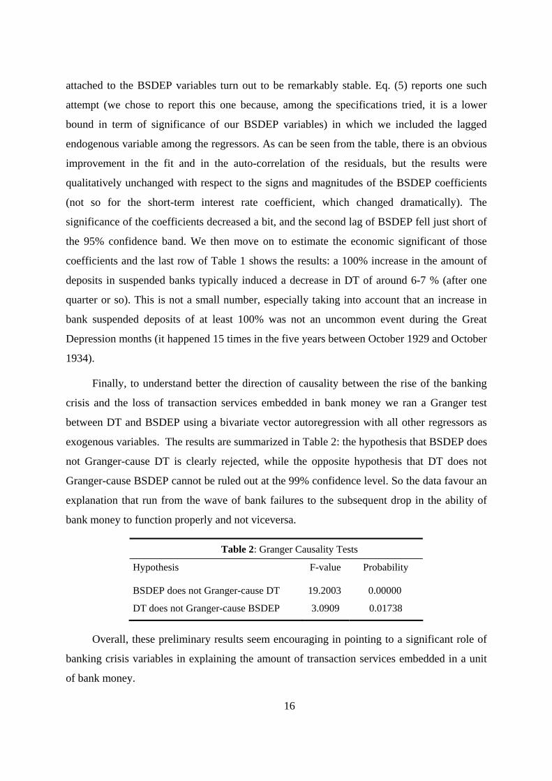
Finally, to understand better the direction of causality between the rise of the banking
crisis and the loss of transaction services embedded in bank money we ran a Granger test
between DT and BSDEP using a bivariate vector autoregression with all other regressors as
exogenous variables. The results are summarized in Table 2: the hypothesis that BSDEP does
not Granger-cause DT is clearly rejected, while the opposite hypothesis that DT does not
Granger-cause BSDEP cannot be ruled out at the 99% confidence level. So the data favour an
explanation that run from the wave of bank failures to the subsequent drop in the ability of
bank money to function properly and not viceversa.
Table 2: Granger Causality Tests
Hypothesis F-value Probability
BSDEP does not Granger-cause DT 19.2003 0.00000
DT does not Granger-cause BSDEP 3.0909 0.01738
Overall, these preliminary results seem encouraging in pointing to a significant role of
banking crisis variables in explaining the amount of transaction services embedded in a unit
of bank money.
17
6. The impact on output of the fall of confidence in bank money
Much more difficult is to show how the drop in the use of bank money due to bank
closures affected aggregate output. The reason is that is hard to construct an empirical test
able to disentangle the effect on income coming from the deterioration in the payment system
from other effects that were running in the same direction (like the “ Bernanke effect”), since
all these competing theories and effects are trying to relate the same ”primary cause” (bank
failures) to the ”final effect” (a fall in real output). The difference lies in the transmission
mechanism invoked.
The historical press of those years is however full of anecdotal evidence in support of
the view that people at the time perceived that, among other factors, the recovery was being
jeopardized by the inefficiency with which transactions were conducted. In an article that
appeared in "The Christian Century" on February 1933 the author wrote:
"It would be a misleading oversimplification of the case to say that the world's present economic condition is wholly the result of dislocations in our system of money and of credit measured in terms of money. But that much of the trouble derives from the inadequacy of the mechanisms of exchange is evidenced by the success which has attended many of the efforts to create cooperative organizations which shall function with little or no use of money and by the direct exchange of commodities or of labor for commodities."
There was also a widespread awareness of the limitations and distortions implicit in the use of alternative media of exchange that were used in substitution for bank money. Commenting on the use of scrip money, many articles point out that their reduced temporal and geographical validity limited the kind of trade that could be accomplished with them. It is thus reasonable to believe that potentially profitable trade opportunities were left unexploited because of that. Many economic agents, like small retailers and businesses, also expressed strong discomfort with the use of scrip money:
"The use of it [scrip money] is one form of inflation, which may be a very good thing at a time when prices are too low. But in view of the contrast which must always exist between scrip and "real money" and the constant danger of a loss of confidence in the former, it is not likely to produce any general rise in the level of prices as measured in terms of legal tender."
18
(The Christian Century, cited)
Usually, the associations which organized the exchanges of goods based on script paid a
premium over cash market prices for the goods exchanged and also imposed a charge to take
care of overhead expenses. The market value of scrip was up to 20 per cent less than cash.14
Stamped money was an evolved version of scrip where a stamp of minimal value (3
cents for a 1$ note) had to be purchased and attached to the note for each transaction. When
enough stamps were attached to the note, it could be redeemed for cash. Their advantage
over scrip laid on greater certainty of duration of its validity, since it circulated until fully
stamped, and of its convertibility at expiration. Again, some comments can be found in the
press that clearly point at possible sources of distortions caused by the use of these media:
"Farmers do not like to take it because the stamp or sales tax is relatively heavy in view of the low prices they get for their products. The same is true in the case of merchants selling products on which the profit margin is small."
(Business Week, January 11 1933, pag.11)
"Merchants refuse to give cash change for purchases amounting to less than the face value because the sales tax on the transaction [the stamp] then becomes heavier. ... The no-change practice stimulates buying somewhat in order to bring the total purchase up to the face value, but it retards circulation." (ibidem)
Finally, banker's and trade acceptances were new financial instruments that were born
and found their first large scale diffusion exactly during the depression years (see Business
Week, June 22, July 20, Sept. 8 1932); they were viewed, rightly, as potential solutions for
expanding credit by “liquefying the great volume of frozen floating commercial debt" and
"unfreeze[ing] a great mass of book credit and accounts receivable by which business is
14 Murray E. King, “Back to Barter”, The New Republic, January 4, 1933.
19
carried on normally and by which it is being retarded at present",15 but it can hardly be argued
that they were ever viewed or used as effective media of exchange.
While mainly anecdotic this evidence clearly show the inconveniences produced by the
deterioration of the functioning of the banking payment system and resulting sharp increase in
transaction costs that came about.
7. Conclusion
In this paper we have argued that the wave of bank failures that took place in the Great
Depression, by increasing the risk of using bank money, induced a “loss of trust” effect. This
in turn translated in higher transaction costs both for those continuing to use bank money and
for those using alternative transaction media. These disruptions in the payment system
entailed real resources costs for the country via the distortions introduced by the existence of
multiple transaction networks and the overall deterioration in the transaction technology
available.
This mechanism is distinct and possibly complementary to those proposed by authors
that have stressed a link between the developments in the financial sector and those in the real
sector. Friedman and Schwartz believe that bank failures were important only because they
contributed to the contraction of money supply, given the restrictive policy of the Fed. We
instead claim that independently from the impact on money supply, which could have been
offset by an increase in money velocity, bank failures, by increasing the probability of
restrictions on the use of bank deposits and the perception of settlement failures, reduced the
acceptability of bank money as a payment medium. The resulting increase in transaction costs
had an impact on consumption and investment. This view is complementary to that of
Bernanke, who points to the impact of financial disruptions on the cost of credit
intermediation resulting from credit rationing. Our thesis is also consistent with the results of
a recent work by Christiano, Motto and Rostagno (2003) who find, by running a dynamic
general equilibrium model, that a liquidity shift (out of bank deposits and into cash) was the
main factor that triggered the crisis.
15 Business Week, June 22, 1932.
20
The empirical tests are consistent with the hypothesis that bank failures affected
people's trust in bank money and led to a sharp fall in the use of bank money as a payment
medium. These findings are somewhat confirmed by anecdotal evidence from the press of the
period which is full of references to the malfunctioning of what we would call today “the
payment system” and to the obstacle that this created to a rapid recovery. While more work is
needed to complete the empirical investigation, we believe that this aspect requires greater
attention, as many of more recent crises may have been amplified by mechanism like the one
we have investigated. It is for instance well known that, during the financial crises in Russia
in 1998 or in Argentina in 2002, the economy suffered not only from the wealth loss induced
by the currency devaluation but also from the disruption in the internal trade due to the
complete lack of trust in the domestic currency as a payment medium, which in many cases
gave rise to exchanges based on barter.
This “loss of confidence” rarely manifests itself but, when it does, it can greatly
exacerbate economic crises. In these circumstances monetary policy is ineffective if not
accompanied by lending of last resort and structural measures. An implication of our analysis
is that central banks can deal more effectively with these episodes of crisis by exercising their
responsibilities with respect to the supervisory and operational role in the payment system.
June 25, 2007
21
References
Angell, James W. (1936), The Behavior of Money: Exploratory Studies, New
York, McGraw-Hill Book Company.
Bernanke, Ben (1983), “Non-monetary effects of the Financial Crisis in the
propagation of the Great Depression”, The American Economic Review, 73.
Calomiris, Charles W. and Joseph R. Mason (2003), “Consequences of Bank
Distress During the Great Depression”, The American Economic Review, 93.
Christiano, Lawrence, R. Motto and M. Rostagno (2004), “The Great
Depression and Friedman-Schwartz Hypothesis”, National Bureau of Economic
Research (Cambridge, MA) Working Paper No.10255.
Field, Alexander J. (1984), “A New Interpretation of the Onset of the Great
Depression”, The Journal of Economic History, 44, no. 2.
Friedman, Milton (1956), “The Quantity of Money - A restatement”, in M.
Friedman (ed.), Studies in the Quantity of Money, Chicago, The University of
Chicago Press.
_____ (1971), "The Lag in Effect of Monetary Policy", in J. Prager (ed.),
Monetary Controversies in Theory and Policy, New York, Random House.
_____ and A. Schwartz (1963), A Monetary History of the United States 1867-
1960, Princeton, Princeton University Press.
Garvy, George (1952), "The Development of Bank Debits and Clearings and
their Use in Economic Analysis", Washington, Board of Governors of the Federal
Reserve System.
____ (1959), Debits and Clearings Statistics and their Use, Washington, Board of
Governors of the Federal Reserve System.
Giannini, Curzio (2004), L’età delle banche centrali, Il Mulino, Bologna 2004.
Haubrich, James (1990), “Non monetary Effects of Financial Crises. Lessons
from the Great Depression in Canada”, Journal of Monetary Economics, 25.
22
Humphrey, David B. (1986), “Payment Finality and Risk in Settlement Failure”,
in A. Sauders and L. White (eds.), Technology and the Regulation of Financial
Markets, Toronto, Lexington Books.
______ (ed.) (1990), The U.S. Payment System: Efficiency, Risk, and the Role of
the Federal Reserve, Proceedings of a Symposium on the US Payment System
sponsored by the Federal Reserve Bank of Richmond, Norwell MA, Kluwer
Academic Publishers.
Klein, Benjamin (1974), “The Competitive Supply of Money”, Journal of
Money, Credit and Banking, 6, no. 4.
Mengle, David (1990), “Legal and regulatory Reforms in Electronic Payments:
an Evaluation of Payment Finality Rules”, in Humphrey (1990).
Rockoff, Hugh (1993), “The Meaning of Money in the Great Depression”,
National Bureau of Economic Research (Cambridge, MA) Historical Paper No.52.
Temin, Peter (1976), Did Monetary Forces Caused the Great Depression ?, New
York, WW Norton & Company Press.
Temin, Peter (1989), Lessons from the Great Depression, Cambridge MA, MIT
University Press
23
Data Appendix
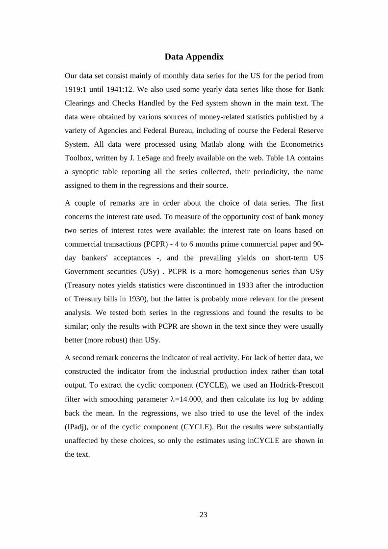
Our data set consist mainly of monthly data series for the US for the period from
1919:1 until 1941:12. We also used some yearly data series like those for Bank
Clearings and Checks Handled by the Fed system shown in the main text. The
data were obtained by various sources of money-related statistics published by a
variety of Agencies and Federal Bureau, including of course the Federal Reserve
System. All data were processed using Matlab along with the Econometrics
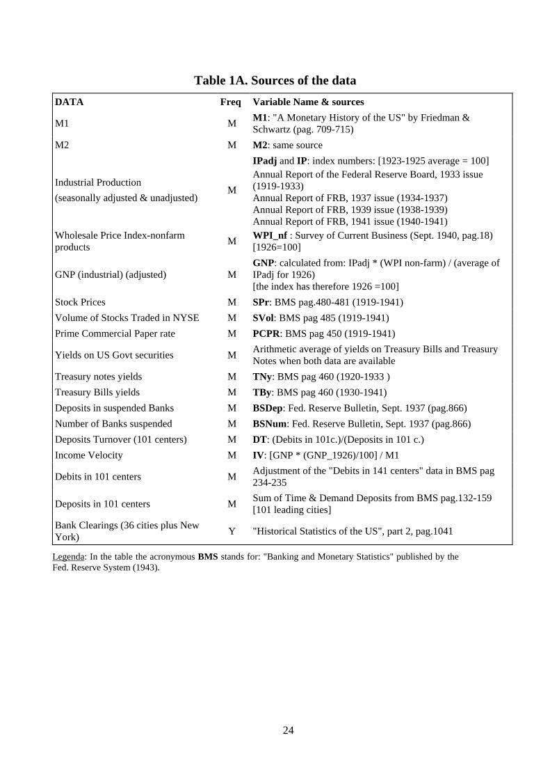
Toolbox, written by J. LeSage and freely available on the web. Table 1A contains
a synoptic table reporting all the series collected, their periodicity, the name
assigned to them in the regressions and their source.
A couple of remarks are in order about the choice of data series. The first
concerns the interest rate used. To measure of the opportunity cost of bank money
two series of interest rates were available: the interest rate on loans based on
commercial transactions (PCPR) - 4 to 6 months prime commercial paper and 90-
day bankers' acceptances -, and the prevailing yields on short-term US
Government securities (USy) . PCPR is a more homogeneous series than USy
(Treasury notes yields statistics were discontinued in 1933 after the introduction
of Treasury bills in 1930), but the latter is probably more relevant for the present
analysis. We tested both series in the regressions and found the results to be
similar; only the results with PCPR are shown in the text since they were usually
better (more robust) than USy.
A second remark concerns the indicator of real activity. For lack of better data, we
constructed the indicator from the industrial production index rather than total
output. To extract the cyclic component (CYCLE), we used an Hodrick-Prescott
filter with smoothing parameter λ=14.000, and then calculate its log by adding
back the mean. In the regressions, we also tried to use the level of the index
(IPadj), or of the cyclic component (CYCLE). But the results were substantially
unaffected by these choices, so only the estimates using lnCYCLE are shown in
the text.
24
Table 1A. Sources of the data DATA Freq Variable Name & sources
M1 M M1: "A Monetary History of the US" by Friedman & Schwartz (pag. 709-715)
M2 M M2: same source
Industrial Production (seasonally adjusted & unadjusted)
M
IPadj and IP: index numbers: [1923-1925 average = 100] Annual Report of the Federal Reserve Board, 1933 issue (1919-1933) Annual Report of FRB, 1937 issue (1934-1937) Annual Report of FRB, 1939 issue (1938-1939) Annual Report of FRB, 1941 issue (1940-1941)
Wholesale Price Index-nonfarm products M WPI_nf : Survey of Current Business (Sept. 1940, pag.18)
[1926=100]
GNP (industrial) (adjusted) M GNP: calculated from: IPadj * (WPI non-farm) / (average of IPadj for 1926) [the index has therefore 1926 =100]
Stock Prices M SPr: BMS pag.480-481 (1919-1941) Volume of Stocks Traded in NYSE M SVol: BMS pag 485 (1919-1941) Prime Commercial Paper rate M PCPR: BMS pag 450 (1919-1941)
Yields on US Govt securities M Arithmetic average of yields on Treasury Bills and Treasury Notes when both data are available
Treasury notes yields M TNy: BMS pag 460 (1920-1933 ) Treasury Bills yields M TBy: BMS pag 460 (1930-1941) Deposits in suspended Banks M BSDep: Fed. Reserve Bulletin, Sept. 1937 (pag.866) Number of Banks suspended M BSNum: Fed. Reserve Bulletin, Sept. 1937 (pag.866) Deposits Turnover (101 centers) M DT: (Debits in 101c.)/(Deposits in 101 c.) Income Velocity M IV: [GNP * (GNP_1926)/100] / M1
Debits in 101 centers M Adjustment of the "Debits in 141 centers" data in BMS pag 234-235
Deposits in 101 centers M Sum of Time & Demand Deposits from BMS pag.132-159 [101 leading cities]
Bank Clearings (36 cities plus New York) Y "Historical Statistics of the US", part 2, pag.1041
Legenda: In the table the acronymous BMS stands for: "Banking and Monetary Statistics" published by the Fed. Reserve System (1943).