Abstract: We estimate a model that summarizes the yield curve using latent factors (specifically, level,slope, and curvature) and also includes observable macroeconomic variables (specifically, real activity,inflation, and the monetary policy instrument). Our goal is to provide a characterization of the dynamicinteractions between the macroeconomy and the yield curve. We find strong evidence of the effects ofmacro variables on future movements in the yield curve and evidence for a reverse influence as well. Wealso relate our results to the expectations hypothesis.
Key Words: Term structure, interest rates, macroeconomic fundamentals, factor model, state-space model
JEL Codes: G1, E4, C5
Acknowledgments: We thank the Editor (Giampiero Gallo) and two referees for insightful guidance. Wethank the Guggenheim Foundation, the National Science Foundation, and the Wharton FinancialInstitutions Center for research support. Finally, we thank Andrew Ang, Pierluigi Balduzzi, Todd Clark,Ron Gallant, Ken Nyholm, Monika Piazzesi, Mike Wickens, Scott Weiner, and discussants andparticipants at many seminars and conferences, for helpful comments. The views expressed in this paperdo not necessarily reflect those of the Federal Reserve Bank of San Francisco.
Macroeconomists, financial economists, and market participants all have attempted to build good
models of the yield curve, yet the resulting models are very different in form and fit. In part, these
differences reflect the particular modeling demands of various researchers and their different motives for
modeling the yield curve (e.g., interest rate forecasting or simulation, bond or option pricing, or market
surveillance). Still, an unusually large gap is apparent between the yield curve models developed by
macroeconomists, which focus on the role of expectations of inflation and future real economic activity in
the determination of yields, and the models employed by financial economists, which eschew any explicit
role for such determinants. This paper takes a step toward bridging this gap by formulating and
estimating a yield curve model that integrates macroeconomic and financial factors.
Many other recent papers have also modeled the yield curve, and they can be usefully categorized
by the extent and nature of the linkages permitted between financial and macroeconomic variables. Many
yield curve models simply ignore macroeconomic linkages. Foremost among these are the popular factor
models that dominate the finance literature – especially those that impose a no-arbitrage restriction. For
example, Knez, Litterman, and Scheinkman (1994), Duffie and Kan (1996), and Dai and Singleton (2000)
all consider models in which a handful of unobserved factors explain the entire set of yields. These
factors are often given labels such as “level,” “slope,” and “curvature,” but they are not linked explicitly
to macroeconomic variables.
Our analysis also uses a latent factor model of the yield curve, but we also explicitly incorporate
macroeconomic factors. In this regard, our work is more closely related to Ang and Piazzesi (2003),
Hördahl, Tristani, and Vestin (2002), and Wu (2002), who explicitly incorporate macro determinants into
multi-factor yield curve models. However, those papers only consider a unidirectional macro linkage,
because output and inflation are assumed to be determined independently of the shape of the yield curve,
but not vice versa. This same assumption is made in the vector autoregression (VAR) analysis of Evans
and Marshall (1998, 2001) where neither contemporaneous nor lagged bond yields enter the equations
driving the economy. In contrast to this assumption of a one-way macro-to-yields link, the opposite view
is taken in another large literature typified by Estrella and Hardouvelis (1991) and Estrella and Mishkin
(1998), which assumes a yields-to-macro link and focuses only on the unidirectional predictive power of
the yield curve for the economy. The two assumptions of these literatures – one-way yields-to-macro or
macro-to-yields links – are testable hypotheses that are special cases of our model and are examined
below. Indeed, we are particularly interested in analyzing the potential bidirectional feedback from the
yield curve to the economy and back again. Some of the work closest to our own allows a feedback from
an implicit inflation target derived from the yield curve to help determine the dynamics of the
macroeconomy, such as Kozicki and Tinsley (2001), Dewachter and Lyrio (2002), and Rudebusch and
-2-
Wu (2003). In our analysis, we allow for a more complete set of interactions in a general dynamic, latent
factor framework.
Our basic framework for the yield curve is a latent factor model, although not the usual no-
arbitrage factor representation typically used in the finance literature. Such no-arbitrage factor models
often appear to fit the cross-section of yields at a particular point in time, but they do less well in
describing the dynamics of the yield curve over time (e.g., Duffee, 2002; Brousseau, 2002). Such a
dynamic fit is crucial to our goal of relating the evolution of the yield curve over time to movements in
macroeconomic variables. To capture yield curve dynamics, we use a three-factor term structure model
based on the classic contribution of Nelson and Siegel (1987), interpreted as a model of level, slope, and
curvature, as in Diebold and Li (2002). This model has the substantial flexibility required to match the
changing shape of the yield curve, yet it is parsimonious and easy to estimate. We do not explicitly
enforce the no-arbitrage restriction. However, to the extent that it is approximately satisfied in the data –
as is likely for the U.S. Treasury bill and bond obligations that we study – it will also likely be
approximately satisfied in our estimates, as our model is quite flexible and gave a very good fit to the
data. Of course, there may be a loss of efficiency in not imposing the restriction of no arbitrage if it is
valid, but this must be weighed against the possibility of misspecification if transitory arbitrage
opportunities are not eliminated immediately.
In section 2, we describe and estimate a basic “yields-only” version of our model – that is, a
model of just the yield curve without macroeconomic variables. To estimate this model, we introduce a
unified state space modeling approach that lets us simultaneously fit the yield curve at each point in time
and estimate the underlying dynamics of the factors. This one-step approach improves upon the two-step
estimation procedure of Diebold and Li (2002) and provides a unified framework in which to examine the
yield curve and the macroeconomy.
In section 3, we incorporate macroeconomic variables and estimate a “yields-macro” model. To
complement the nonstructural nature of our yield curve representation, we also use a simple nonstructural
VAR representation of the macroeconomy. The focus of our examination is the nature of the linkages
between the factors driving the yield curve and macroeconomic fundamentals.
In section 4, we relate our framework to the expectations hypothesis, which has been studied
intensively in macroeconomics. The expectation hypotheses of the term structure is a special case of our
model that receives only limited support.
We offer concluding remarks in section 5.
2. A Yield Curve Model Without Macro Factors
1 As described in documentation from the Bank for International Settlements (1999), manycentral banks have adopted the Nelson-Siegel yield curve (or some slight variant) for fitting bond yields.
2 Our Nelson-Siegel yield curve (1) corresponds to equation (2) of Nelson Siegel (1987). Theirnotation differs from ours in a potentially confusing way: they use m for maturity and for theconstant .
3 More precisely, Diebold and Li show that corresponds to the negative of slope astraditionally defined (“long minus short yields”). For ease of discussion, we prefer simply to call , andhence , “slope,” so we define slope as “short minus long.”
-3-
In this section, we introduce a factor model of the yield curve without macroeconomic variables,
which is useful for two key reasons. First, methodologically, such a model proves to be a convenient
vehicle for introducing the state-space framework that we use throughout the paper. Second, and
substantively, the estimated yields-only model serves as a useful benchmark to which we subsequently
compare our full model that incorporates macroeconomic variables.
2.1 A Factor Model Representation
The factor model approach expresses a potentially large set of yields of various maturities as a
function of just a small set of unobserved factors. Denote the set of yields as , where J denotes
maturity. Among practitioners and especially central banks,1 a very popular representation of the cross-
section of yields at any point in time is the Nelson and Siegel (1987) curve:
(1)
where are parameters.2 Moreover, as shown by Diebold and Li (2002), the Nelson-
Siegel representation can be interpreted in a dynamic fashion as a latent factor model in which , ,
and are time-varying level, slope, and curvature factors and the terms that multiply these factors are
factor loadings.3 Thus, we write
(2)
where Lt, St, and Ct are the time-varying , , and . We illustrate this interpretation with our
empirical estimates below.
If the dynamic movements of Lt, St, and Ct follow a vector autoregressive process of first order,
4 As is well-known, ARMA state vector dynamics of any order may be readily accommodated instate-space form. We maintain the VAR(1) assumption only for transparency and parsimony.
-4-
then the model immediately forms a state-space system.4 The transition equation, which governs the
dynamics of the state vector, is
(3)
. The measurement equation, which relates a set of N yields to the three unobservable
factors, is
(4)
. In an obvious vector/matrix notation, we write this state-space system as
(5)
. (6)
For linear least squares optimality of the Kalman filter, we require that the white noise transition and
measurement disturbances be orthogonal to each other and to the initial state:
(7)
-5-
(8)
(9)
In much of our analysis, we assume that the H matrix is diagonal and the Q matrix is non-diagonal. The
assumption of a diagonal H matrix, which implies that the deviations of yields of various maturities from
the yield curve are uncorrelated, is quite standard. For example, in estimating the no-arbitrage term
structure models, i.i.d. “measurement error” is typically added to the observed yields. This assumption is
also required for computational tractability given the large number of observed yields used. The
assumption of an unrestricted Q matrix, which is potentially non-diagonal, allows the shocks to the three
term structure factors to be correlated.
In general, state-space representations provide a powerful framework for analysis and estimation
of dynamic models. The recognition that the Nelson-Siegel form is easily put in state-space form is
particularly useful because application of the Kalman filter then delivers maximum-likelihood estimates
and optimal filtered and smoothed estimates of the underlying factors. In addition, the one-step Kalman
filter approach of this paper is preferable to the two-step Diebold-Li approach, because the simultaneous
estimation of all parameters produces correct inference via standard theory. The two-step procedure, in
contrast, suffers from the fact that the parameter estimation and signal extraction uncertainty associated
with the first step is not acknowledged in the second step. Finally, the state-space representation paves
the way for possible future extensions, such as allowance for heteroskedasticty, missing data, and heavy-
tailed measurement errors, although we do not pursue those extensions in the present paper.
At this point, it is also perhaps useful to explicitly contrast our approach with others that have
been used in the literature. A completely general (linear) model of yields would be an unrestricted VAR
estimated for a set of yields. One potential drawback to such a representation is that the results may
depend on the particular set of yields chosen. A factor representation, as above, can aggregate
information from a large set of yields. One straightforward factor model is a VAR estimated with the
principal components formed from a large set of yields. (See Evans and Marshall 1998, 2001for VAR
term structure analyses.) Such an approach restricts the factors to be orthogonal to each other but does
not restrict the factor loadings at all. In contrast, our model allows correlated factors but restricts the
factor loadings through limitations on the set of admissible yield curves. For example, the Nelson-Siegel
form guarantees positive forward rates at all horizons and a discount factor that approaches zero as
maturity increases. Such economically-motivated restrictions likely aid in the analysis of yield curve
5 Accumulated experience – as well as formal Bayes/Stein theory – leads naturally to thecelebrated parsimony or shrinkage principle as a strategy for avoiding data mining and in-sampleoverfitting. This is the broad insight that imposition of sensible restrictions, which must of coursedegrade in-sample fit, is often a crucial ingredient for the production of useful models for analysis andforecasting.
6 For details of Kalman filtering and related issues such as initialization of the filter, see Harvey(1981) or Durbin and Koopman (2001).
-6-
dynamics.5 Alternative restrictions could also be imposed. The most popular alternative is the no-
arbitrage restriction, which enforces the consistency of the evolution of the yield curve over time with the
absence of arbitrage opportunities. However, there is mixed evidence on the extent to which these
restrictions enhance inference. (Compare, for example, Ang and Piazzesi, 2003 and Duffee, 2002.)
2.2 Yields-Only Model Estimation
We examine U.S. Treasury yields with maturities of 3, 6, 9, 12, 15, 18, 21, 24, 30, 36, 48, 60, 72,
84, 96, 108 and 120 months. The yields are derived from bid/ask average price quotes, from January
1972 through December 2000, using the unsmoothed Fama-Bliss (1987) approach, as described in
Diebold and Li (2002). They are measured as of the beginning of each month; this timing convention is
immaterial for the yields-only model but will be more important when macro variables are introduced.
As discussed above, the yields-only model forms a state-space system, with a VAR(1) transition
equation summarizing the dynamics of the vector of latent state variables, and a linear measurement
equation relating the observed yields to the state vector. Several parameters must be estimated. The
(3x3) transition matrix A contains 9 free parameters, the (3x1) mean state vector contains 3 free
parameters, and the measurement matrix contains 1 free parameter, . Moreover, the transition and
disturbance covariance matrix Q contains 6 free parameters (one disturbance variance for each of the
three latent level, slope and curvature factors and three covariance terms), and the measurement
disturbance covariance matrix H contains seventeen free parameters (one disturbance variance for each of
the seventeen yields). All told, then, 36 parameters must be estimated by numerical optimization – a
challenging, but not insurmountable, numerical task.
For a given parameter configuration, we use the Kalman filter to compute optimal yield
predictions and the corresponding prediction errors, after which we proceed to evaluate the Gaussian
likelihood function of the yields-only model using the prediction-error decomposition of the likelihood.
We initialize the Kalman filter using the unconditional mean (zero) and unconditional covariance matrix
of the state vector.6 We maximize the likelihood by iterating the Marquart and Berndt-Hall-Hall-
Hausman algorithms, using numerical derivatives, optimal stepsize, and a convergence criterion of
7 Recall that we define slope as short minus long, so that a negative mean slope means that yieldstend to increase as maturity lengthens.
8 Not surprisingly, when we estimate the model with the restriction that the Q matrix is diagonal,the point estimates and standard errors of the elements of the A matrix are little changed from Table 1.
9 As an additional check of model adequacy, we also tried four-factor and five-factor extendedmodels, as in Björk and Christensen (1999). The extensions provided negligible improvement in modelfit. These results are consistent with Dahlquist and Svensson (1994) who compare the Nelson and Siegelmodel with a more complex functional form and also find no improvement to using the latter.
-7-
for the change in the norm of the parameter vector from one iteration to the next. We impose non-
negativity on all estimated variances by estimating log variances; then we convert to variances by
exponentiating and compute asymptotic standard errors using the delta method. We obtain startup
parameter values by using the Diebold-Li two-step method to obtain the initial transition equation matrix,
initializing all variances at 1.0, and initializing at the value given in Diebold and Li (2002).
In the first panel of Table 1 we present estimation results for the yields-only model. The estimate
of the A matrix indicates highly persistent own dynamics of , , and , with estimated own-lag
coefficients of .99, .94 and .84, respectively. Cross-factor dynamics appear unimportant, with the
exception of a minor but statistically significant effect of on . The estimates also indicate that
persistence decreases (as measured by the diagonal elements of A), and transition shock volatility
increases (as measured by the diagonal elements of Q), as we move from to to . The remaining
estimates appear sensible; the mean level is approximately 8 percent, the mean slope is approximately -
1.5 percent, and the mean curvature is insignificantly different from 0.7 In the second and third panel of
Table 1 we report the estimated Q matrix and two tests of its diagonality. There is only one individually-
significant covariance term, and the off-diagonal elements of the matrix (tested jointly as a group) are
only marginally significant.8 Finally, the estimated of .077 implies that the loading on the curvature
factor is maximized at a maturity of 23.3 months.
The yields-only model fits the yield curve remarkably well. The first two columns of Table 2
contain the estimated means and standard deviations of the measurement equation residuals, expressed in
basis points, for each of the seventeen maturities that we consider. The mean error is negligible at all
maturities (with the possible exception of 3 months), and in the crucial middle range of maturities from 6
to 60 months, the average standard deviation is just 8.7 basis points. The average standard deviation
increases at very short and very long maturities but nevertheless remains quite small.9
We use the Kalman smoother to obtain optimal extractions of the latent level, slope and curvature
factors. In Figure 1, we plot these three estimated factors together for comparative assessment, and in
10 In each case, the latent factor extractions are based on full-sample parameter estimates.
11 More precisely, the correlation between Hodrick-Prescott “cycles” (deviations from trends) in and is 0.55, and the correlation between Hodrick-Prescott “trends” in and is -0.07.
-8-
Figures 2, 3, and 4 we plot the respective factors in isolation of each other, but together with various
empirical proxies and potentially related macroeconomic variables.10
The level factor displays very high persistence in Figure 1and is of course positive – in the
neighborhood of 8 percent. In contrast, the slope and curvature are less persistent and assume both
positive and negative values. The unconditional variances of the slope and curvature factors are roughly
equal but are composed differently: slope has higher persistence and lower shock variance, whereas
curvature has lower persistence and higher shock variance. Interestingly, slope and curvature appear
related at business cycle frequencies. The simple correlation is 0.25, but the correlation at business cycle
frequencies is 0.55 and at very low frequencies is -0.07.11
In Figure 2 we show the estimated level and two closely-linked comparison series: a common
empirical proxy for level (namely, an average of short-, medium- and long-term yields,
), and a measure of inflation (the 12-month percent change in the price deflator
( ) for personal consumption expenditures, namely, ). The high .80 correlation
between and supports our interpretation of as a level factor. The
correlation between and actual inflation, which is .43, is consistent with a link between the level of the
yield curve and inflationary expectations, as suggested by the Fisher equation. This link is a common
theme in the recent macro-finance literature, including Kozicki and Tinsley (2001), Dewachter and Lyrio
(2002), Hördahl, Tristani, and Vestin (2002), and Rudebusch and Wu (2003).
In Figure 3 we show the estimated slope and two comparison series, to which the slope factor is
closely linked: a standard empirical slope proxy ( ), and an indicator of macroeconomic
activity (demeaned capacity utilization). The high .98 correlation between and lends
credibility to our interpretation of as a slope factor. The correlation between and capacity
utilization, which is .39, suggests that yield curve slope, like yield curve level, is intimately connected to
the cyclical dynamics of the economy.
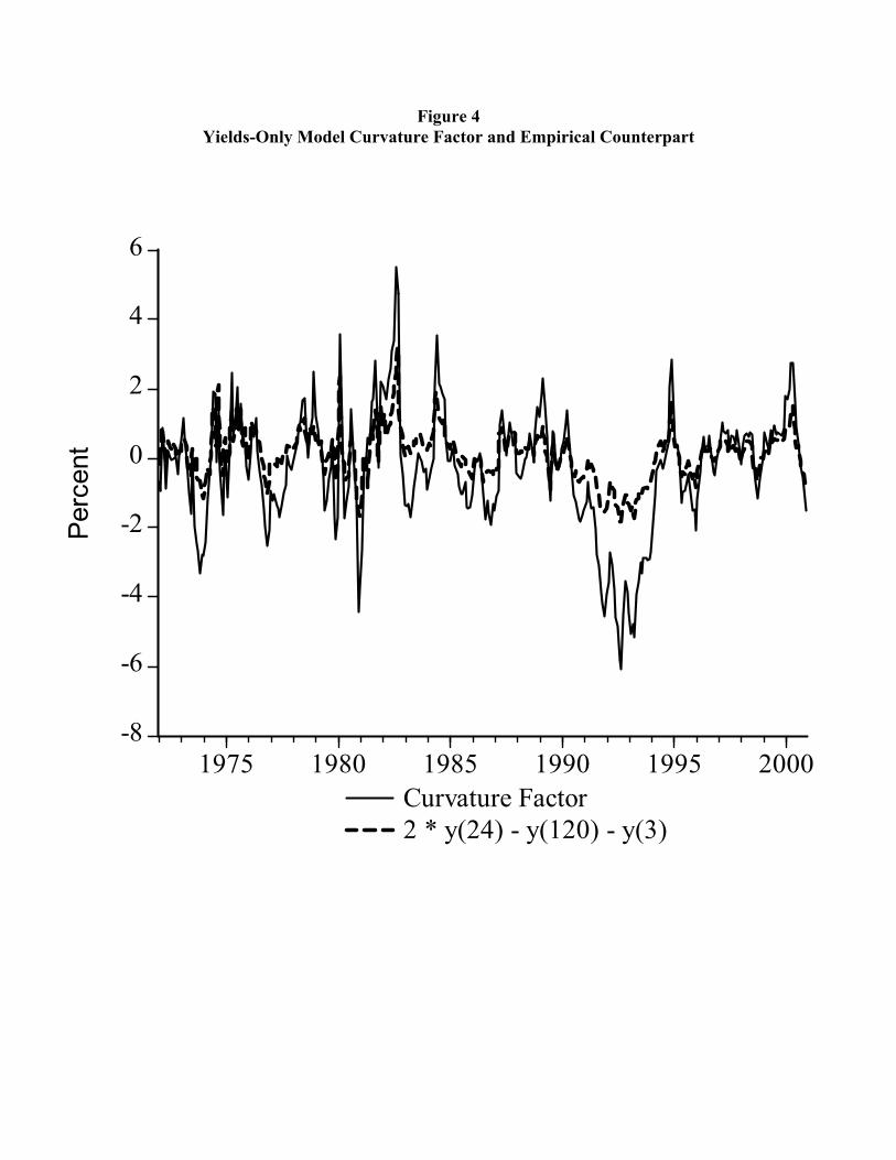
Finally, in Figure 4 we show the estimated curvature together with a standard empirical curvature
proxy, , to which is closely linked with a correlation of .96, which again lends
credibility to our interpretation of as a curvature factor. Unfortunately, as shown in our combined
yields-macro model in the next section, we know of no reliable macroeconomic links to .
3. A Yield Curve Model With Macro Factors
12 The variable INFL is the 12-month percent change in the price deflator for personalconsumption expenditures, and FFR is the monthly average funds rate.
13 See, for example, Rudebusch and Svensson (1999) and Kozicki and Tinsley (2001).
14 7 is now Nx6, but the three rightmost columns contain only zeros, so that the yields still loadonly on the yield curve factors. This form is consistent with the view that only three factors are needed todistill the information in the yield curve.
-9-
Given the ability of the level, slope, and curvature factors to provide a good representation of the
yield curve, it is of interest to relate them to macroeconomic variables. This can be done readily in an
expanded version of the above state-space framework. In the next five subsections, we analyze the
dynamic interactions between the macroeconomy and the yield curve, and we assess their importance.
3.1 The Yields-Macro Model: Specification and Estimation
We wish to characterize the relationships among and the macroeconomy. Our
measures of the economy include three key variables: manufacturing capacity utilization ( ), the
federal funds rate ( ), and annual price inflation ( ).12 These three variables represent,
respectively, the level of real economic activity relative to potential, the monetary policy instrument, and
the inflation rate, which are widely considered to be the minimum set of fundamentals needed to capture
basic macroeconomic dynamics.13
A straightforward extension of the yields-only model adds the three macroeconomic variables to
the set of state variables and replaces equations (5)-(7) with
( )
( )
, ( )
where and the dimensions of A, and Q are increased as
appropriate.14 This system forms our yields-macro model, to which we will compare our earlier yields-
15 We have maintained a first-order VAR structure for simplicity and tractability. However,based on some limited exploration of second-order models, it appears that our results are robust to thisassumption as well.
16 As discussed below, we also examined the robustness of our results to alternative identificationstrategies. In particular, we obtained similar results for a model with a diagonal Q matrix, which is neutralwith respect to ordering of the variables. We also obtained similar results using end-of-period yield dataand ordering the variables as , , , .
17 The own-lag coefficient of rounds to 1.00 but actually is just less than one, and stationarityis assured since the largest eigenvalue of the A matrix is 0.98.
-10-
only model.15 Our baseline yields-macro model continues to assume a non-diagonal Q matrix and a
diagonal H matrix. Producing impulse responses from this model requires an identification of the
covariances given by the off-diagonal elements of the Q matrix. Following common practice, we do this
by assuming a particular recursive causal ordering of the variables; namely, we order the variables
, , , . We order the term structure factors prior to the macro variables because they are
dated at the beginning of each month.16
In the first panel of Table 3 we display the estimates of the parameters of the yields-macro model,
which contains the crucial macro and term structure interactions.17 Individually, many of the off-diagonal
elements appear insignificant; however, as we discuss below, key blocks of coefficients appear jointly
significant. The estimated Q matrix is provided in the second panel of Table 3. Several of the off-
diagonal covariances appear significant individually. The Wald and Likelihood Ratio tests reported in the
third panel clearly reject the diagonality of the Q matrix.
The time series of estimates of the level, slope, and curvature factors in the yields-macro model
are very similar to those obtained in the yields-only model. Thus, as shown in the third and fourth
columns of Table 2, the means and standard deviations of the measurement errors associated with the
yields-macro model are essentially identical to those of the yields-only model. In particular, the mean
errors are again negligible, and in the important 6- to 60-month maturity range, the average standard
deviation is just 8.6 basis points.
3.2 Macroeconomic and Yield Curve Impulse Response Functions
We examine the dynamics of the complete yields-macro system by via impulse response
functions, which we show in Figure 5, along with ninety percent confidence intervals. We will consider
four groups of impulse responses in turn: macro responses to macro shocks, macro responses to yield
curve shocks, yield curve responses to macro shocks, and yield curve responses to yield curve shocks.
The responses of the macro variables to macro shocks match the typical impulse responses
18 The interpretation of the persistence of FFR – the policy rate manipulated by the Fed – is opento some debate. However, Rudebusch (2002) argues that it does not indicate “interest rate smoothing” or“monetary policy inertia”; instead, it reflects serially correlated unobserved factors to which the Fedresponds.
19 There is a marginally-significant initial upward response of inflation to the funds rate – a so-called “price puzzle” – which is typical in small VARs of this kind.
20 An ex post does not appear to be appropriate, as a positive shock to inflation doesnot boost economic activity (see Rudebusch and Svensson, 1999).
-11-
produced in small estimated macro models of the kind commonly used in monetary policy analysis (e.g.,
Rudebusch and Svensson, 1999). The macro variables all show significant persistence.18 In addition, an
increase in the funds rate depresses capacity utilization over the next few years, similar to the aggregate
demand response in Rudebusch and Svensson (1999). The funds rate, in turn, rises with capacity
utilization and – albeit with only marginal significance – with inflation in a fashion broadly consistent
with an estimated Federal Reserve monetary policy reaction function. Finally, inflation exhibits a clear
aggregate supply response to increased capacity utilization and, over time, declines in response to a funds
rate increase.19
The yield curve components add some interesting elements to the macro responses. The macro
variables have negligible responses to shocks in the curvature factor. In contrast, an increase in the slope
factor is followed by an almost one-to-one response in the funds rate. That is, there is a close connection
between the slope factor and the instrument of monetary policy. However, there are two interpretations of
such a connection. On the one hand, the Fed may be reacting to yields (which are measured at the
beginning of the month) in setting the funds rate. On the other hand, given the institutional frictions of
monetary policy decision-making (e.g., the 6-week spacing between policy meetings and the requirement
for committee approval), it is likely that yields are reacting to macroeconomic information in anticipation
of Fed actions. That is, to the extent the Fed has established a predictable policy reaction function to
macroeconomic information, movements in bond markets may often appear to predate those of the Fed.
Finally, an increase in the level factor raises capacity utilization, the funds rate, and inflation.
Recall from Figure 2 the close connection between inflation and the level factor. The macro responses
exhibited in Figure 5 are consistent with the above interpretation of the level factor as the bond market’s
perception of long-run inflation. Under this interpretation, an increase in the level factor – that is, an
increase in future perceived inflation – lowers the ex ante real interest rate when measured as ,
which is followed by a near-term economic boom.20 However, during our sample, the Fed has apparently
accommodated only a small portion of the expected rise in inflation. The nominal funds rate rises
21 Gurkaynak, Sack, and Swanson (2003) and Rudebusch and Wu (2003) discuss such amechanism.
22 Overall then, in important respects, this analysis improves on the usual monetary VAR, whichcontains a flawed specification of monetary policy (Rudebusch, 1998). In particular, the use of level,slope, and the funds rate allows a much more subtle and flexible description of policy.
-12-
significantly in response to the level shock, damping utilization, and limiting the rise in inflation to only
about 40% of the initial shock to the level.
Now consider the response of the yield curve to the macro variables. While the curvature factor
shows very little response, the slope factor responds directly to positive shocks in all three macro
variables. For example, an increase in the funds rate almost immediately pushes up the slope factor so the
yield curve is less positively sloped (or more negatively sloped). Positive shocks to utilization, and to a
lesser extent inflation, also induce similar though more delayed movements in the tilt. These reactions are
consistent with a monetary policy response that raises the short end of the term structure in response to
positive output and inflation surprises. However, shocks to the macro variables also affect the level of the
term structure. In particular, surprises to actual inflation appear to give a long-run boost to the level
factor. Such a reaction is consistent with long-inflation expectations not being firmly anchored, so a
surprise increase in inflation (or even in real activity) feeds through to an expectation of higher future
inflation, which raises the level factor.21 A positive shock to the funds rate is also followed by a small
temporary jump in the level factor. In principle, a surprise increase in the monetary policy rate could
have two quite different effects on inflation expectations. On the one hand, if the central bank has a large
degree of credibility and transparency, then a tightening could indicate a lower inflation target and a
likely lowering of the level factor. Alternatively, a surprise tightening could indicate that the central back
is worried about overheating and inflationary pressures in the economy – news that would boost future
inflation expectations and the level factor. Evidently, over our sample, the later effect has dominated.
Finally, consider the block of own-dynamics of the term structure factors. The three factors
exhibit significant persistence. Most off-diagonal responses are insignificant; however, a surprise
increase in the level factor, which we interpret as higher inflation expectations, is associated with
loosening of policy as measured by the slope factor and a lowering of the short end of the term structure
relative to the long end.22
3.3 Macroeconomic and Yield Curve Variance Decompositions
Variance decompositions provide a popular metric for analyzing macro and yield curve
interactions. Table 4 provides variance decompositions of the 1-month, 12-month, and 60-month yields
23 This result is consistent with the tilt of the yield curve being driven by counter-cyclicalmonetary policy, as in Rudebusch and Wu (2003).
-13-
at forecast horizons of 1, 12, and 60 months. Decompositions are provided for both the yields-only and
the yields-macro models. At a 1-month horizon, very little of the variation in rates is driven by the macro
factors (8, 4, and 2 percent for the 1-month, 12-month, and 60-month yield, respectively). This suggests a
large amount of short-term idiosyncratic variation in the yield curve that is unrelated to macroeconomic
fundamentals. However, at longer horizons, the macro factors quickly become more influential, and at a
60-month horizon, they account for about 40 percent of the variation in rates. This contribution is similar
to the results in Ang and Piazzesi’s (2003) macro model. A comparison of yields-only and yields-macro
decompositions shows that the variance accounted for by the slope factor falls notably with the addition
of the macro variables. That is, movements in yields that had been attributed to shocks to slope are now
traced to shocks to output, inflation, and monetary policy.23 In contrast, the variance contributions from
level and curvature are little changed on balance.
Table 5 examines the variance decompositions for the macroeconomic variables based on the
joint yields-macro model and a “macro-only” model, which is a simple first-order VAR for CU, FFR,
INFL. In the yields-macro model, the term structure factors account for very little of the variation in
capacity utilization or inflation. Yield curve factors do predict a substantial fraction of movements in the
funds rate, but as noted above, this may reflect the adjustment of bond markets to new information before
the Fed can react.
Taken together, the variance decompositions suggest that the effects of the yield curve on the
macro variables are less important than the effects of the macro variables on the yield curve. To interpret
this result correctly, it is important to note that an interest rate – the federal funds rate – is also included
among the macro variables. That is, we are asking what would the yield curve add to a standard small
macro model, such as the Rudebusch-Svensson (1999) model. We are not arguing that interest rates do
not matter, but that, for our specification and sample, the funds rate is perhaps, to a rough approximation,
a sufficient statistic for interest rate effects in macro dynamics, which is a conclusion consistent with Ang,
Piazzesi, and Wei (2003).
3.4 Formal Tests of Macro and Yield Curve Interactions
The coefficient matrix A and the covariance matrix Q shown in Table 3 are crucial for assessing
interactions between macroeconomic variables and the term. We begin by partitioning the 6x6 A matrix
into four 3x3 blocks, as
-14-
(12)
and similarly for the 6x6 Q matrix,
(13)
where the superscript T denotes transpose. We attribute all the covariance given by the block to the
effect of yield curve variables on the macro variables, as the latter come before the former in the recursive
ordering we employ. As such, there are two links from yields to the macroeconomy in our setup: the
contemporaneous link given by , and the effects of lagged yields on the macroeconomy embodied in
. Conversely, links from the macroeconomy to yields are embodied in .
We report in Table 6 the results of likelihood ratio and Wald tests of several key restrictions on
the A and Q matrices. Both tests overwhelmingly reject the “no interaction” hypothesis of
. Interestingly, less severe restrictions allowing for unidirectional but not bidirectional
links are similarly rejected. In particular, we reject both the hypothesis of “no macro to yields” link
( ) and the hypothesis of “no yields to macro” link ( ). We conclude that there is clear
statistical evidence in favor of a bidirectional link between the macroeconomy and the yield curve.
3.5 Robustness to an Alternative Identification Strategy
Our results above are based on a recursive ordering of the variables. In this section we estimate a
version of the macro-yields model with a diagonal Q matrix. Imposition of the diagonality constraint
allows us to sidestep issues of structural identification and highlight macro-finance linkages, without
being tied to particular orderings or other identification schemes, which have been so contentious in the
so-called “structural” VAR literature. In Table 7, we provide estimates of A and the diagonal elements of
Q, which are very close to those reported in Table 3. Next we repeat the linkage tests and report the
results in Table 8. Because we now maintain the assumption of diagonal Q throughout, the hypotheses
tested correspond to restrictions only on the A matrix. Interestingly, we find considerably less evidence in
favor of a yields to macro link than in the “non-diagonal Q” case reported in Table 6: the Wald test
statistic of the null hypothesis of no yields to macro link has a p-value of 0.19.
We also compute the impulse responses for this version of the model. In Figure 6 we show both
point and interval estimates of the impulse responses from the earlier-reported non-diagonal Q version of
the yields-macro model, along with the point estimates of the impulse responses from the diagonal Q
version for comparison. With only one or two exceptions out of 36 impulse response functions (the
responses of capacity utilization and funds rate to a shock in slope), the differences are negligible. The
-15-
same is of course also true for the variance decompositions, which we show for the diagonal Q model in
Table 9, and which are close to those reported earlier for the non-diagonal Q version, with the possible
exception of the significantly lower contribution of yield curve variables to the variation in the funds rate.
This result is in line with the weak yield-to-macro linkage already documented for this version of the
model.
4. Examining The Expectations Hypothesis
It is useful to contrast our representation of the yield curve with others that have appeared in the
literature. Here we relate our yield curve modeling approach to the traditional macroeconomic approach
based on the expectations hypothesis.
The expectations hypothesis of the term structure states that movements in long rates are due to
movements in expected future short rates. Any term or risk premia are assumed to be constant through
time. In terms of our notation above, which pertains to the pure discount bond yields in our data set, the
theoretical bond yield consistent with the expectations hypothesis is
(14)
where c is a term premium that may vary with the maturity but assumed to be constant through time.
The expectations hypothesis has long been a key building block in macroeconomics both in
casual inference and formal modeling (see, for example, Fuhrer and Moore, 1995, or Rudebusch, 1995).
However, various manifestations of the failure of the expectations hypothesis have been documented at
least since Macaulay (1938). Campbell and Shiller (1991) and Fuhrer (1996) provide recent evidence on
the failure of the expectations hypothesis, and we use their methodology to examine it in the context of
our model. Specifically, we compare the theoretical bond yields, , constructed via (14) under the
assumption that the expectations hypothesis holds, with the actual bond yields . We construct the
expected future 1-month yields by iterating forward the estimated yields-macro model using equation (5')
and the measurement equation (6') for , and then we compute the theoretical bond yields at each
point in time using equation (14).
In Figure 7, we show for six maturities (m = 3, 12, 24, 36, 60, 120) the theoretical yields implied
by the expectations hypothesis, together with the actual yields. As in Fuhrer (1996), throughout our
sample there are large deviations between the theoretical and actual yields, especially at longer
24 Not surprisingly, a formal statistical test along the lines of Krippner (2002) rejects therestrictions placed by the expectations hypothesis on the yields-macro model.
-16-
maturities.24 Nevertheless, the actual and theoretical rates move together most of the time. Over the
entire sample, for example, the correlation between the actual 10-year and 1-month yield spread,
, and the theoretical spread, , is .60. Furthermore, during certain periods
the actual and theoretical rates move very closely together. This partial success of the expectations
hypothesis is consistent with Fuhrer (1996) and Kozicki and Tinsley (2001), who argue that much of the
apparent failure of the expectations hypothesis reflects the assumption of a constant Fed reaction function
– and in particular a constant inflation target – over the entire sample. Indeed, the expectations
hypothesis fits much better during the second half of the sample, when inflation expectations were likely
better anchored.
5. Summary and Conclusions
We have specified and estimated a yield curve model that incorporates both yield factors (level,
slope, and curvature) and macroeconomic variables (real activity, inflation, and the stance of monetary
policy). The model’s convenient state-space representation facilitates estimation, the extraction of latent
yield-curve factors, and testing of hypotheses regarding dynamic interactions between the macroeconomy
and the yield curve. Interestingly, we find strong evidence of macroeconomic effects on the future yield
curve and somewhat weaker evidence of yield curve effects on future macroeconomic developments.
Hence, although bi-directional causality is likely present, effects in the tradition of Ang and Piazzesi
(2003) seem relatively more important than those in the tradition of Estrella and Hardouvelis (1991),
Estrella and Mishkin (1998), and Stock and Watson (2000). Of course, market yields do contain
important predictive information about the Fed’s policy rate. We also relate our yield curve modeling
approach to a traditional macroeconomic approach based on the expectations hypothesis. The results
indicate that the expectations hypothesis may hold reasonably well during certain periods, but that it does
not hold across the entire sample.
From a finance perspective, our analysis is unusual in that we do not impose no-arbitrage
restrictions. However, such an a priori restriction may in fact be violated in the data due to illiquidity in
thinly-traded regions of the yield curve, so imposing it may be undesirable. Also, if the no-arbitrage
restriction does indeed hold for the data, then it will at least approximately be captured by our fitted yield
curves, because they are flexible approximations to the data. Nevertheless, in future work, we hope to
derive the no-arbitrage condition in our framework and explore whether its imposition is helpful for
forecasting, as suggested by Ang and Piazzesi (2003).
-17-
Appendix
Calculation of Impulse Response Functions and Variance Decompositions
In this appendix, we describe the computation of the impulse response functions (IRFs) and
variance decompositions (VDs) for our models. All models in the paper can be written in VAR(1) form,
(A1)
where is an vector of endogenous variables, is the constant vector and is the transition
matrix. The residuals follow
(A2)
where is a (potentially non-diagonal) variance-covariance matrix. In order to find the IRFs and VDs,
we must write the VAR(1) in moving average (MA) form. Letting denote the identity matrix,
the unconditional mean of is , and we can write the system as
(A3)
Assuming that satisfies the conditions for covariance stationarity, we can write the MA representation
of the VAR as
(A4)
where and for
A.1. Impulse-Response Functions
We define the IRF of the system as the responses of the endogenous variables to one unit shocks
in the residuals. One would often see responses to a “one standard deviation” shock instead of the “one
unit” shock that we use. Because all the variables we use in our analysis are in percentage terms we find
it more instructive to report results from one percentage point shocks to the residuals.
A.1.1 Diagonal
The response of to a one unit shock to is
(A5)
where is the (i,j) element of the corresponding matrix. To compute the asymptotic standard errors
of the IRFs, we follow Lütkepohl (1990). Let and . Suppose that
(A6)
Then the asymptotic distribution of the IRFs can be derived using
(A7)
where
-18-
(A8)
A.1.2 Non-Diagonal
When is non-diagonal, we cannot compute the IRFs using the original residuals, . We use a
Cholesky decomposition to obtain a lower-triangular matrix that satisfies to define .
The transformed residuals have an identity covariance matrix, .
The response of to a one unit shock to is
(A9)
where is the jth column of and is the (j, j) element of the original variance covariance matrix.
To compute the asymptotic standard errors of the IRFs, assume that (A6) holds where now
. Denote by a matrix whose (i, j)th element is the response of the ith variable in period t
to a one standard deviation shock to the jth variable in period t-k; that is, the jth column of is given by
. Then the asymptotic distribution of can be derived using
(A10)
where
(A11)
(A12)
(A13)
is a matrix such that , is a matrix such that , and
is as defined in (A8).
A.2. Variance Decompositions
The contribution of the jth variable to the mean squared error (MSE) of the s-period-ahead
forecast, under the assumption of diagonal is
(A14)
while for the non-diagonal case it is
(A15)
The MSE is given by
(A16)
where both MSE and are matrices. We define the VD at horizon s as the fraction of MSE of
the ith variable due to shocks to the jth variable:
(A17)
where and denote the (i,i) elements of the respective matrices.
To compute the VD of the yields, we combine the result above with the measurement equation
for the yields,
-19-
(A18)
where and follow from equation (1). The contribution of the jth variable to the MSE of the s-
period ahead forecast of the yield at maturity is given by
(A19)
where we assume that the factors and are the first three elements of the vector . Similarly, the
MSE of the s-period ahead forecast of the yield at maturity is given by
(A20)
and the VD of the yield with maturity is the MSE of the yield due to the jth variable at horizon s:
(A21)
-20-
References
Ang, A. and Piazzesi, M. (2003), “A No-Arbitrage Vector Autoregression of Term Structure Dynamicswith Macroeconomic and Latent Variables,” Journal of Monetary Economics, 50, 745-787.
Ang, A., Piazzesi, M. And Wei, M. (2003), “What Does the Yield Curve Tell us About GDP Growth?,”manuscript, Columbia University and UCLA.
Bank for International Settlements (1999), “Zero-Coupon Yield Curves: Technical Documentation,” Bankfor International Settlements, Switzerland.
Björk, T. and Christensen, B. (1999), “Interest Rate Dynamics and Consistent Forward Rate Curves,”Mathematical Finance, 9, 323-348.
Brousseau, V. (2002), “The Functional Form of Yield Curves,” Working Paper 148, European CentralBank.
Campbell, J.Y. and R.J. Shiller (1991), “Yield Spreads and Interest Rate Movements: A Bird’s EyeView,” Review of Economic Studies, 57, 495-514.
Dahlquist M. and L.E.O. Svensson (1996), “Estimating the Term Structure of Interest Rates for MonetaryPolicy Analysis,” Scandinavian Journal of Economics, 98, 163-183.
Dai Q. and Singleton, K. (2000), “Specification Analysis of Affine Term Structure Models,” Journal ofFinance, 55, 1943-1978.
Dewachter, H. and Lyrio, M. (2002), “Macroeconomic Factors in the Term Structure of Interest Rates,”Manuscript, Catholic University Leuven and Erasmus University Rotterdam.
Diebold, F.X. and Li., C. (2002), “Forecasting the Term Structure of Government Bond Yields,”Manuscript, Department of Economics, University of Pennsylvania.
Duffee, G. (2002), “Term Premia and Interest Rate Forecasts in Affine Models,” Journal of Finance, 57,405-443.
Duffie, D. and Kan, R. (1996), “A Yield-Factor Model of Interest Rates,” Mathematical Finance, 6,379-406.
Durbin, J. and S.J. Koopman (2001), Time Series Analysis by State Space Methods. Oxford: OxfordUniversity Press..
Estrella, A. and Hardouvelis, G.A. (1991), “The Term Structure as a Predictor of Real EconomicActivity,” Journal of Finance, 46, 555-576.
Estrella, A. and Mishkin, F.S. (1998), “Predicting U.S. Recessions: Financial Variables as LeadingIndicators,” Review of Economics and Statistics, 80, 45-61.
Evans, C.L. and Marshall, D. (1998), “Monetary Policy and the Term Structure of Nominal InterestRates: Evidence and Theory,” Carnegie-Rochester Conference Series on Public Policy, 49, 53-
-21-
111.
Evans, C.L. and Marshall, D. (2001), “Economic Determinants of the Nominal Treasury Yield Curve,”Manuscript, Federal Reserve Bank of Chicago.
Fama, E. and Bliss, R. (1987), “The Information in Long-Maturity Forward Rates,” American EconomicReview, 77, 680-692.
Fuhrer, J. (1996), “Monetary Policy Shifts and Long-Term Interest Rates,” The Quarterly Journal ofEconomics, 1183-1209.
Fuhrer, J., and G. Moore (1995), “Monetary Policy Trade-Offs and the Correlation Between NominalInterest Rates and Real Output,” American Economic Review 85, 219-239.
Gurkaynak, R.S., Sack, B., and Swanson E. (2003), “The Excess Sensitivity of Long-Term Interest Rates:Evidence and Implications for Macroeconomic Models,” Manuscript, Federal Reserve Board.
Harvey, A.C. (1981), Time Series Models (Second Edition, 1993). Cambridge: MIT Press.
Hördahl, P., Tristani, O. and Vestin, D. (2002), “A Joint Econometric Model of Macroeconomic andTerm Structure Dynamics,” Manuscript, European Central Bank.
Knez, P., Litterman, R. and Scheinkman, J. (1994), “Exploration into Factors Explaining Money MarketReturns,” Journal of Finance, 49, 1861-1882.
Kozicki, S. and Tinsley, P.A. (2001), “Shifting Endpoints in the Term Structure of Interest Rates,”Journal of Monetary Economics, 47, 613-652.
Krippner, L. (2002), “The OLP Model of the Yield Curve: A New Consistent Cross-sectional andIntertemporal Approach,” manuscript, Victoria University of Wellington.
Lütkepohl, H. (1990), “Asymptotic Distributions of Impulse Response Functions and Forecast ErrorVariance Decompositions of Vector Autoregressive Models,” Review of Economics andStatistics, 72, 116-125.
Macaulay, F.R. (1938), Some Theoretical Problems Suggested by the Movements of Interest Rates, BondYields, and Stock Prices in the United States Since 1856, (New York: NBER).
Nelson, C.R. and Siegel, A.F. (1987), “Parsimonious Modeling of Yield Curves,” Journal of Business,60, 473-489.
Rudebusch, G.D. (1995), “Federal Reserve Interest Rate Targeting, Rational Expectations, and the TermStructure,” Journal of Monetary Economics 35, 245-274.
Rudebusch, G.D. (1998), “Do Measures of Monetary Policy in a VAR Make Sense?,” InternationalEconomic Review 39, 907-931.
Rudebusch, G.D. (2002), “Term Structure Evidence on Interest Rate Smoothing and Monetary PolicyInertia,” Journal of Monetary Economics 49, 1161-1187.
-22-
Rudebusch, G.D. and Svensson, L.E.O. (1999), “Policy Rules for Inflation Targeting,” in J.B. Taylor(ed.), Monetary Policy Rules. Chicago: University of Chicago Press, 203-246.
Rudebusch, G.D. and Wu, T. (2003), “A Macro-Finance Model of the Term Structure, Monetary Policy,and the Economy,” Manuscript, Federal Reserve Bank of San Francisco.
Stock, J.H. and Watson, M.W. (2000), “Forecasting Output and Inflation: The Role of Asset Prices,”Manuscript, Kennedy School of Government, Revised January 2003.
Wu, T. (2002), “Monetary Policy and the Slope Factors in Empirical Term Structure Estimations,”Federal Reserve Bank of San Francisco Working Paper 02-07.
0.99 0.03 -0.02 8.02(0.01) (0.01) (0.01) (1.67)
-0.03 0.94 0.04 -1.44(0.02) (0.02) (0.03) (0.60)
0.03 0.02 0.84 -0.42(0.03) (0.02) (0.03) (0.54)
0.09 -0.01 0.04(0.01) (0.01) (0.02)
0.38 0.01(0.03) (0.03)
0.80(0.07)
Test Statistic P-Value6.75 0.087.65 0.05
Likelihood RatioWaldNote: Both test statistics are Chi-square with 3 degrees of freedom.
Table 1Yields-Only Model Parameter Estimates
Tests for Diagonality of Q Matrix
Notes: Bold entries denote parameter estimates significant at the 5 percent level. Standard errors appear in parentheses.
Estimated Q Matrix
Notes: Each row presents coefficients from the transition equation for the respective state variable. Bold entries denote parameter estimates significant at the 5 percent level. Standard errors appear in parentheses.
µ
tL
tS
tC
1−tL 1−tS 1−tC
tL
tS
tC
tL tS tC
Mean Standard Deviation Mean Standard Deviation3 -12.64 22.36 -12.53 22.216 -1.34 5.07 -1.26 4.849 0.49 8.11 0.54 8.15
Notes: We report the means and standard deviations of the measurement errors, expressed in basis points, for yields of various maturities measured in months.
Table 2
Yields-Only Model Yields-Macro ModelMaturity
Summary Statistics for Measurement Errors of Yields
0.00Note: Both test statistics are Chi-square with 15 degrees of freedom.
Tests for Diagonality of Q Matrix
Wald
Test Statistic307.89209.21
Table 3
Estimated Q Matrix
P-Value
Yields-Macro Model Parameter Estimates
Notes: Each row presents coefficients from the transition equation for the respective state variable. Bold entries denote parameter estimates significant at the 5 percent level. Standard errors appear in parentheses.
Likelihood Ratio 0.00
Notes: Bold entries denote parameter estimates significant at the 5 percent level. Standard errors appear in parentheses.
Notes: Each entry is the proportion of the forecast variance (at the specified forecast horizon) for a 1-, 12- or 60-month yield that is explained by the particular factor.
Notes: Each entry is the proportion of the forecast variance (at the specified forecast horizon) for capacity utilization, funds rate and inflation that is explained by the particular factor.
Table 5
Yields-Macro Model
CU
FFR
INFL
Macro-Only Model
Macro-Only Model
No Interaction No Macro to Yields No Yields to MacroA2 = 0, A3 = 0 and Q2 = 0 A2 = 0 A3 = 0 and Q2 = 0
Number of Restrictions 27 9 18Likelihood Ratio Statistic 362.11 107.13 258.66
Notes: p -values appear in parentheses. A2, A3 and Q2 refers to the relevant blocks of A and Q matrices as explained in the text. All test statistics in each column is a Chi-squared with the degrees of freedom equal to the number of restrictions.
Notes: Each row represents the transition equation for the respective state variable. Bold entries denote parameter estimates significant at the 5 percent level. Standard errors appear in parentheses.
Notes: Each entry is the proportion of the forecast variance (at the specified forecast horizon) for a 1-, 12- or 60-month yield and capacity utilization, funds rate and inflation that is explained by the particular factor.