The Mass Assembly History of Field Galaxies Thesis by Kevin Bundy In Partial Fulfillment of the Requirements for the Degree of Doctor of Philosophy California Institute of Technology Pasadena, California 2006 (Submitted February 23)
The history of galaxy evolution is a story that can be told in two ways. The work
presented in this thesis contributes to one of these narratives, which begins with the
birth of galaxies in the early universe and tells the history of their evolution to the
present day. Before describing some key questions still unanswered in this story and
how the present work addresses them, it is helpful to consider the second perspec-
tive, namely the history of our understanding of galaxies. As an introduction, this
historical perspective is valuable for two reasons. First, unlike our current scientific
description, the history of the subject—at least to the present day—is much less likely
to change. And second, this history illuminates broad patterns of progress that help
orient our current picture and provide insight into the future of the subject.
1.1 A Historical Perspective on Galaxy Evolution
Although the modern understanding of galaxy formation and evolution is only about
30 years old, the subject has a history that stretches back several centuries. From
the beginning, the subject, like many other scientific pursuits, has found its way
forward under the sometimes opposing pressures of theoretical insight and new ob-
servations driven by advancing technologies. Arguably, it was theoretical deduction
that launched the study of external galaxies about 150 years after Kepler’s work on
planetary orbits. In 1755, Immanuel Kant, before moving on to problems of a dif-
ferent scale, described a prescient cosmology in Universal History and Theory of the
2
Heavens (Kant orig. 1755), first identifying a model describing the Milky Way as a
disk of stars with the sun located in the plane and then making the leap to predicting
the existence and appearance of other such systems:
If a system of fixed stars which are related in their positions to the common
plane as we have delineated the Milky Way to be, be so far removed from
us that the individual stars of which it consists are no longer sensibly
distinguishable even by the telescope ... then this world will appear under
a small angle as a patch of space whose figure will be circular if its plane
is presented directly to the eye, and elliptical if it is seen from the side or
obliquely.1
Kant’s ideas were supported by William Herschel, often considered the first extra-
galactic astronomer because of his visual sky survey and “Book of Sweeps” in which
he cataloged thousands of sources with particular interest in so-called “nebulae” that
he believed were located beyond the galaxy. Whether these nebulae were the same
as Kant’s “Island Universes” was not seriously tested until the early 20th century
when a number of new observations were originally understood to discount the the-
ory. Catalogs of hundreds of thousands of spiral nebulae demonstrated how their
distribution avoided the plane of the Milky Way, which suggested that the nebulae
were physically associated with our galaxy. The spiral appearance of many of these
nebulae supported the recent work on collapsing clouds of gas by Jeans, and the de-
velopment of spectroscopy confirmed that many of the nebulae consisted of heated
gas in emission. On the other hand, similar measurements showed the spectra of
some nebulae like M31 to be star-like, and novae—understood to be associated with
exploding stars—were observed in the spiral arms of others (see the review by Smith
1982).
The controversy culminated in the “Great Debate” between Harlow Shapley and
Heber Curtis in 1920, with Shapley using his maps of globular cluster Cepheid vari-
1We are lucky that Kant wrote on this subject early in his career and before adopting a stylethat led to such sentences as, “the conception of right does not take into consideration the matterof the matter of the act of will in so far as the end which any one may have in view in willing it isconcerned.”
3
ables to argue for a “Big Galaxy” picture of the Milky Way with no need for island
universes. Cepheid variables soon solved the problem, but in favor of Curtis, with
the detection of Cepheids at extragalactic distances in NGC 6822, as announced by
Hubble at the American Astronomical Society meeting in 1925 (see Hubble 1925).
With the establishment of “nebulae” as extragalactic objects, attention focused on
using them as tracers of the large-scale mass distribution and evolution of the universe.
The goal was to determine which cosmological “world model” correctly described
how the universe was expanding. Caught in the flow of this expansion, galaxies
could be used to trace its evolution, but early on it was appreciated that variations
in the intrinsic luminosity of galaxies would make their utility as distance markers
challenging (e.g., Sandage 1961). It was therefore necessary to understand and model
the luminosity evolution of galaxies. Aided by newly available computers, Tinsley
developed the first detailed models of the stellar populations of galaxies of various
types and predicted how they would evolve (e.g., Tinsley 1972). This important tool
helped provide an empirically motivated model for understanding observations.
At the same time, rapid theoretical progress, much of it driven by the work of
Peebles and Zeldovich in the 1960’s, was taking place in reconciling the Big Bang
theory with the evolution of structure in the universe and the growth of galaxies.
The basic principle was that galaxies formed through the development of initial mat-
ter overdensities, imprinted as random fluctuations in the power spectrum after the
Big Bang. Press & Schechter (1974) developed a linear formalism for tracking these
fluctuations and showed how self-similar mass distributions matching the observed
structure among galaxies could be achieved with a hierarchical, “bottom-up” frame-
work. The general behavior of gas collapse, cooling, and dissipation in the peaks of
the density distribution was explored in several landmark papers in the late 1970’s
(e.g., Rees & Ostriker 1977; Silk 1977; White & Rees 1978) that set the foundation for
our modern picture of how galaxies form out of the neutral gas in the early universe.
4
1.1.1 Faint Number Counts and Galaxy Redshift Surveys
In a way reminiscent of the relationship between Kant’s prediction of island universes
and their eventual confirmation, it has taken 30 years of intense observations and ad-
ditional theoretical developments for this hierarchical worldview of galaxy formation
to gain acceptance. Indeed, through the late 1970’s and into the 1980’s indisputable
evidence for evolution in the galaxy population could not even be firmly established.
Butcher & Oemler (1978) showed evidence for a changing number of blue galaxies in
distant clusters, but studies of the field population2 were at first restricted to photo-
graphic magnitude number counts (Tyson & Jarvis 1979; Peterson et al. 1979) and
spectroscopic surveys limited in both magnitude and redshift (Turner 1980; Gunn
1982; Kirshner et al. 1983; Peterson et al. 1986). Of these two, number counts proved
more valuable at the time for probing distant galaxies. The advent of CCDs enabled
very deep observations (e.g. BJ < 25, Tyson 1988) that confirmed evidence for an
excess in the number counts above Tinsley-like models with no evolution (Figure 1.1).
Number count studies continued into the early 1990’s, with particular interest in K-
band counts because of the smaller k-corrections and uncertainties due to dust in this
waveband. Early reviews on the topic of number magnitude counts are provided in
Koo & Kron (1992) and Ellis (1997).
The results from number counts provided tantalizing evidence for evolution in the
galaxy population but were inherently limited because the observed galaxies could
not be located in redshift space. The need was clear, and a new era of distant galaxy
redshift surveys was launched with the work by Broadhurst et al. (1988). Using
the Anglo Australian Telescope equipped with a multi-object, fiber-fed spectrograph,
Broadhurst et al. (1988) surveyed 187 galaxies to bJ < 21.5. Although they found ev-
idence for an increase in the fraction of blue, star-forming field galaxies with redshift,
the observed redshift distribution was consistent with no-evolution models, seemingly
2This period also saw other exciting developments in galaxy studies, including observations ofclustering and spatial distribution characteristics (Tonry & Davis 1979; Davis & Peebles 1983),continuing efforts to understand galaxies in clusters (e.g., Dressler 1980), and the identification ofscaling relations (e.g., Faber & Jackson 1976; Tully & Fisher 1977; Kormendy 1977). The reviewhere will focus, however, on efforts to understand the distant field population.
5
Figure 1.1 A compilation of number magnitude counts in the B and K band fromEllis (1997). The samples come from Metcalfe et al. (1996) and Moustakas et al.(1997). Dashed lines are power-law fits to the data, while the solid lines indicateno-evolution predictions. The K-band counts have been offset by +1 dex for clarity.
in contradiction with expectations from number counts. The same general pattern
was also found in Colless et al. (1990), whose Low Dispersion Sky Survey (LDSS)
utilized multi-slit spectroscopy to observe 149 galaxies one magnitude fainter than
Broadhurst et al. (1988).
Though demonstrating evolution, these first results did not agree with the in-
terpretation of the significant faint excess in the number counts. More ambitious
surveys making use of new telescopes and instrumentation soon followed with the
hope of addressing the problem. The Canada-France Redshift Survey (Lilly et al.
1995a) measured 730 galaxies to z ∼ 1, showing strong differential evolution in the
luminosity function (Figure 1.2) with a brightening of blue galaxies at z >∼ 0.5, while
the red population was observed to barely evolve (Lilly et al. 1995b). The Autofib
Survey (Ellis et al. 1996) obtained 1700 spectroscopic redshifts and showed similar
results, including a steepening of the B-band luminosity function with redshift and
stronger evolution among galaxies with inferred star formation (based on detected
OII emission, Ellis et al. 1996) as well as late spectral type (Heyl et al. 1997). Work
in the Hawaii Deep Fields (Cowie et al. 1996) added K-band photometry to 393 spec-
6
troscopic redshifts, providing the first evidence for a decrease in the typical mass of
star-forming galaxies with time—a phenomenon they called “downsizing.”
As discussed in the review by Ellis (1997), these first large spectroscopic surveys
greatly increased our understanding of the evolving galaxy population and luminosity
function out to z <∼ 1, but like earlier redshift surveys (Broadhurst et al. 1988; Colless
et al. 1990) still left the puzzle of the excess faint galaxies unsolved. The resolution
of this problem came from three developments. First, part of the discrepancy was
mitigated by improved local studies of the luminosity function (e.g., Lin et al. 1996;
Marzke & da Costa 1997; Bromley et al. 1998; Lin et al. 1999; Cross et al. 2001)
that revealed a steeper faint-end slope, implying that less evolution was needed to
explain the faint counts (this problem was discussed in Ellis 1997). Second, a non-
zero cosmological constant, Λ, became an increasingly popular way of reconciling low
values of Ωb with inflationary constraints that required Ωtot = 1 as well as explain-
ing evidence for accelerated expansion from supernovae type Ia studies (Riess et al.
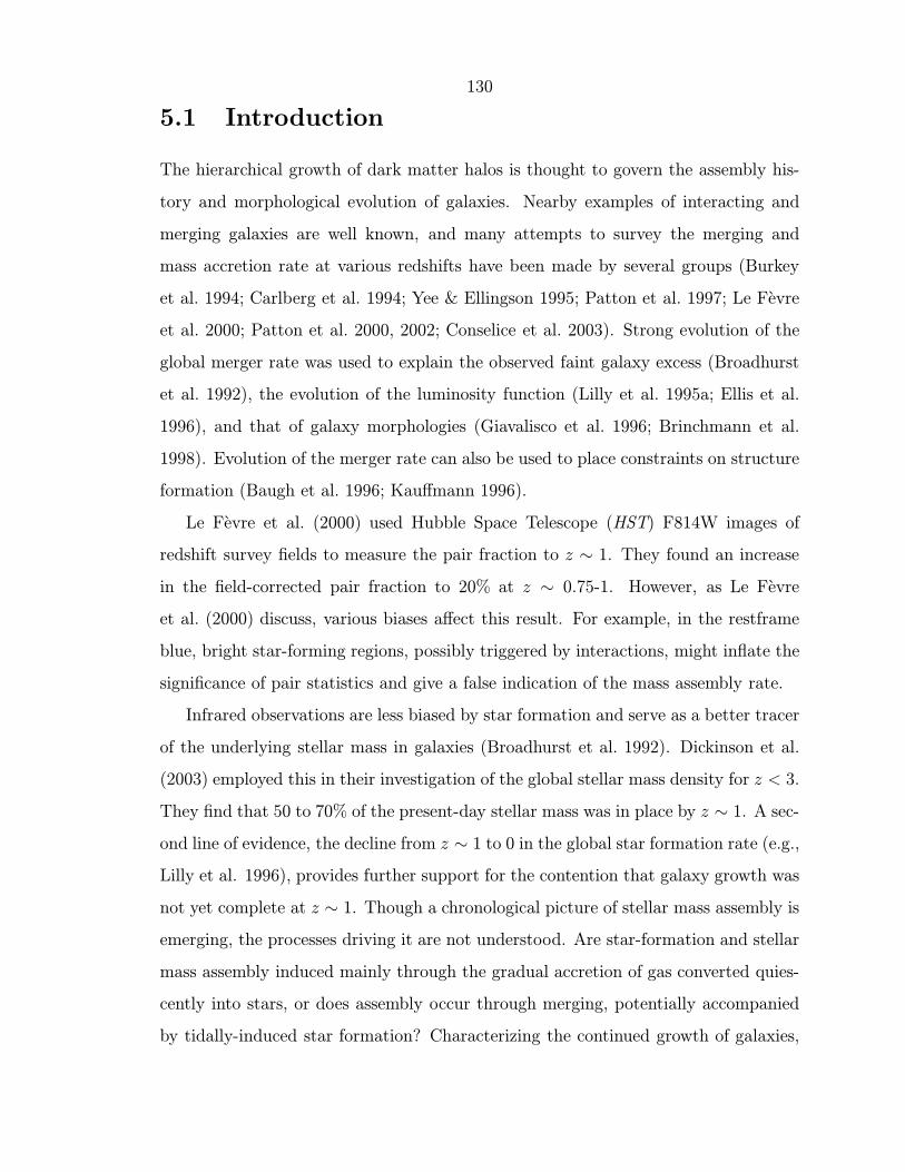
1998). Fukugita et al. (1990) had shown early on that the larger volumes and ages
of cosmological models with Λ > 0 could more easily accommodate the faint galaxy
number counts. Finally, the perception of how galaxies evolve had begun to change.
The predominant view had been one in which galaxies form from an early collapse
(Eggen et al. 1962) and evolve in isolation (Tinsley 1972), exemplified in this quote
on faint galaxy studies from a lecture by Kron (Kron 1993):
The term “galaxy evolution” is used universally in this context, but “galaxy
aging” might better describe the phenomenon we are looking for.
However, by the early 1990’s, the hierarchical framework developed by Peebles and
its formulation in the Cold Dark Matter (CDM) paradigm (e.g., Blumenthal et al.
1984; Davis et al. 1985; Bardeen et al. 1986) had been incorporated into the first semi-
analytic models (White & Frenk 1991) that were capable of matching the observations.
The notion that galaxies merge (i.e., violation of number conservation) at relatively
late times found increasing acceptance in the community (e.g., Carlberg & Charlot
1992; Carlberg 1992) and helped explain the faint blue excess as the progenitors of
7
Figure 1.2 Red and blue luminosity functions at different redshifts taken from Lillyet al. (1995a). The “best estimate” luminosity functions are shown. For z > 0.2, thesolid curve traces a Schechter function fit. The dashed curve reproduces the resultobtained for the 0.2 < z < 0.5 redshift bin, and the dotted line is the local, combinedluminosity function from Loveday et al. (1992).
8
merging systems.
The resolution of the faint blue galaxy problem represents a shift in thinking about
galaxy formation. At the very least, it highlights the necessity for accurate z = 0
benchmarks such as the luminosity and mass functions to which high-z observations
can be compared. It also marks a new era of cosmology defined by a nonzero cosmo-
logical constant. But, perhaps most important, it reinforces a dynamic perspective
of galaxies, which, in accordance with CDM predictions, emphasizes the role of inter-
actions in shaping the properties of galaxies and the importance of mass assembly as
the driving mechanism behind their growth.
1.1.2 The Cosmic Star Formation History
While the spectroscopic surveys of the mid-1990’s were exploring the luminosity func-
tion of the field population to z ∼ 1, two new developments helped to outline the
evolution of the global star formation rate (SFR) to redshifts as high as z ∼ 5. The
first was tracing the evolving luminosity density of the universe and fitting it with
models of the integrated luminosity of the star-forming population. With the very
deep imaging afforded by Hubble Space Telescope (HST) observations, and especially
the Hubble Deep Field (HDF, Williams et al. 1996), as well as the addition of photo-
metric redshifts (e.g., Sawicki et al. 1997), this technique was used to constrain the
global SFR to z ∼ 5 (e.g., Lilly et al. 1996; Madau et al. 1996, 1998). Consistent
with interpretations based on the global production of metals (e.g., Pei & Fall 1995),
numerous subsequent papers confirmed the general trends found in this work (see
Figure 1.3), namely an order of magnitude rise in the SFR with redshift to z ∼ 1
with a peak at z ∼ 1–2 followed by an uncertain but apparently moderate decline at
higher redshifts (see the review by Hopkins 2004).
The second development, the location and characterization of the star-forming
Lyman break population at z ∼ 3, supported this picture of an enhanced cosmic
SFR at early times. Through spectroscopic follow-up conducted at Keck Observa-
tory, Steidel and collaborators not only confirmed the high redshifts of Lyman break
9
Figure 1.3 A compilation of the global SFR density as measured by numerous authorsfrom Hopkins (2004). The solid curve shows a fit to the data. The dotted curvespresent models and the dashed line delineates expectations from spectral studies oflocal galaxies.
galaxies (LBGs) but presented evidence that they were massive systems undergoing
significant star formation and were likely to be the progenitors of present-day massive
ellipticals (Steidel et al. 1996; Giavalisco et al. 1996). Furthermore, by extending such
work to higher redshifts, Steidel et al. (1999) demonstrated that an equally vigorous
amount of star formation was exhibited by LBGs even at z ∼ 4. This established the
presence of a high rate of cosmic star formation at very early times, as illustrated in
Figure 1.3.
These new constraints on the cosmic star formation history provided a valuable
benchmark for models of galaxy formation that incorporated hierarchical merging
(e.g., Cole et al. 2000) and “collisional starbursts” (e.g., Somerville et al. 2001) in or-
10
der to describe the substantial increase in the SFR at early times. At the same time,
studies at z <∼ 1 with HST found significant evolution in morphology and evidence
for galaxy interactions that supported expectations for the hierarchical framework.
Hubble imaging was added to spectroscopic surveys to constrain the luminosity func-
tion and number counts of morphological populations (e.g., Driver et al. 1995a,b;
Abraham et al. 1996; Brinchmann et al. 1998; Driver et al. 1998) which demonstrated
the increasing abundance of star-forming irregular galaxies and a higher incidence
of merging (Burkey et al. 1994; Driver et al. 1998; Le Fevre et al. 2000) at early
times. In the context of the global SFR, these observations seemed to be probing the
final stages of the active period at z ∼ 2. They suggested that the decrease in the
blue luminosity density—and, hence, the cosmic SFR—was driven by a decline in the
merger rate exemplified by the decreasing abundance of irregular star-forming galax-
ies. Thus, in support of the hierarchical scenario, it appeared that galaxy assembly
was responsible for driving evolution and governing the rate of star formation in the
universe.
1.1.3 The Era of Galaxy Mass Studies
In recent years, models based on the CDM (or now ΛCDM) framework such as the
one described in Cole et al. (2000) have become increasingly successful at reproducing
the observed cosmic SFR and luminosity function to z ∼ 1. But while work on the
evolution of galaxy luminosity has continued to the present day (e.g., Cohen 2002;
Wolf et al. 2003; Willmer et al. 2005; Faber et al. 2005; Ilbert et al. 2005), the results
of such efforts are difficult to interpret in physical terms and do not place strong
additional constraints on models of galaxy formation. This limitation of optical galaxy
tracers was recognized and described by Brinchmann & Ellis (2000):
To make progress, we require an independent “accounting variable” capa-
ble of tracking the likely assembly and transformation of galaxies during
the interval 0 < z < 1. The color and emission-line characteristics are
transient properties and poorly suited for this purpose ... The dynamical
11
Figure 1.4 The evolution in the global stellar mass density of E/S0’s, spirals, andpeculiars defined by visual HST morphology (from Brinchmann & Ellis 2000). Theshaded regions show predictions from simple merger models.
or stellar mass is the obvious choice.
If reliable galaxy mass estimates can be obtained, it is possible to move beyond
luminosity measurements and apply comprehensive tests to the CDM paradigm by
comparing the expected hierarchical assembly of dark matter to the observed assembly
history of galaxy mass.
Brinchmann & Ellis (2000) employed a novel technique that utilizes K-band pho-
tometry to estimate the stellar masses of galaxies (this tool is a critical aspect of the
work presented in this thesis and is described in detail in Chapter 2). In this way,
they were able to probe the mass assembly of morphological populations, demonstrat-
ing how the global mass density of late-type galaxies has declined since z ∼ 1, while
that of spheroidals has grown (Figure 1.4)—a process suggestive of transformation
between the two populations.
12
Arguably, this important result marks the beginning of a new approach to the
subject that benefits from investigating the mass-dependent evolution and assembly
of galaxies. While modern studies of high-z dynamical masses (e.g., Bohm et al. 2004;
Treu et al. 2005b) and gravitational lens galaxies (Bolton et al. 2005) are coming
online, the promise of this approach is also a large part of the motivation for ground-
based near-infrared (near-IR) surveys, many of which are further described in Chapter
2 (e.g., Saracco et al. 1997, 1999; McCracken et al. 2000; Huang et al. 2001; Drory
et al. 2001; Chen et al. 2002; Cimatti et al. 2002; Fontana et al. 2003; Abraham et al.
2004), as well as stellar masses derived from Spitzer Space Telescope observations at
z > 1 (e.g., Shapley et al. 2005; Papovich et al. 2005).
1.2 The Mass Assembly History of Field Galaxies
As described in the previous section, the end of the last decade saw an enormous
increase in our knowledge about galaxy evolution with an accompanying shift toward
a merger-driven ΛCDM framework as a means of interpreting observations. While
successful in a variety of ways, many unanswered questions remain in our understand-
ing.
• When do galaxies of a given mass assemble their stellar content? Does the rate
of assembly agree with ΛCDM predictions?
• What causes the significant decline in the global SFR?
• How important is merging in the assembly of galaxies and what role does it
play in their evolution?
• What causes the bimodality in the galaxy distribution? How are properties
such as color, star formation rate, morphology, and mass related? How do they
evolve with time?
The work presented in the chapters that follow addresses these questions through
an investigation of the stellar masses of distant galaxies. Ideally, it would be possible
13
to characterize the assembly of galaxies beginning at very high redshifts and indeed
significant progress has occurred in this area (e.g., Juneau et al. 2005; Reddy et al.
2005; Shapley et al. 2005; Papovich et al. 2005; Chapman et al. 2005; van Dokkum
et al. 2006). In this thesis, however, I will concentrate on the interval 0 < z <∼ 1.5,
which, although it may not include the most active epochs of galaxy formation, is
accessible to new spectroscopic and near-IR instruments that enable detailed, multi-
wavelength studies of statistically complete samples covering a large dynamic range
in mass. The primary goal is a detailed account of the mass assembly history of
galaxies over this redshift interval. A plan of the thesis follows.
1.2.1 The Infrared Survey at Palomar: Observations and
Methods for Determining Stellar Mass
Brinchmann & Ellis (2000) showed the power of combining K-band photometry, op-
tical imaging, and spectroscopic redshifts in surveys of evolving populations. Further
progress required much larger samples so that the broad patterns in the global stellar
mass density (e.g., Cowie et al. 1996; Brinchmann & Ellis 2000; Cohen 2002) could
be broken down and studied in terms of the galaxy mass function. As described in
Chapter 2, this was the inspiration for an extensive near-IR campaign I undertook at
Palomar Observatory. After 65 nights over nearly three years, I present an unprece-
dented sample of over 12,000 galaxies with spectroscopic redshifts (0.2 < z < 1.5)
from the DEEP2 Galaxy Redshift Survey (Davis et al. 2003) and Palomar Ks-band
photometry down to Ks ≈ 20.5 (Vega).
Chapter 2 also describes the method I developed for utilizing near-IR plus op-
tical photometry to estimate the stellar masses of galaxies. This key tool figures
prominently in all of the work presented in this thesis.
14
1.2.2 The Mass Assembly History of Morphological Popula-
tions
The impact of HST observations on the study of galaxy morphology and evolution
was discussed in §1.1.2. These studies demonstrated how the Hubble Sequence, which
provides a reliable rubric for classifying the morphology of galaxies at z = 0, begins to
break down at z >∼ 1 (e.g., Conselice et al. 2004). The increased SFR at these epochs
suggests a link to morphology that is further supported by the higher frequency of
bright, blue late-type galaxies at early times. In addition, Brinchmann & Ellis (2000)
showed evidence for the possible transformation of late-types into spheroidal systems
based on the evolving stellar mass density of these populations. While theoretical ex-
pectations suggested that merging can lead to spheroidal configurations (e.g., Barnes
& Hernquist 1991), details on the nature of this transformation were not known.
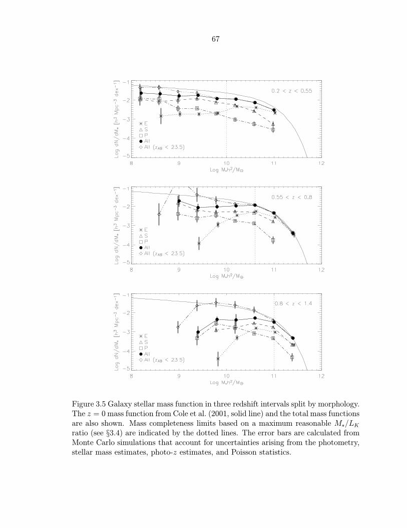
Chapter 3 presents a study (Bundy et al. 2005a) utilizing observations in the
GOODS fields from HST, Palomar, and Keck observatories to address these issues. By
charting the galaxy stellar mass function of ellipticals, spirals, and irregular galaxies
out to z ∼ 1, we extended the work of Brinchmann & Ellis (2000) and showed that
ellipticals dominate at the highest masses even at early times, indicative of an early
formation time for the most massive galaxies. Below a stellar mass of 2–3×10¹⁰M⊙,
the galaxy population becomes dominated by late-type systems. This transition mass
is not only very similar to the bimodal division as traced by various parameters in
the z = 0 population (e.g., Kauffmann et al. 2003b), but also appears to be higher at
z ∼ 1. This, combined with our observation of very little evolution in the total mass
function, suggests that the mechanism driving morphological evolution operates on a
mass scale that shifts downward with time, a phenomenon we refer to as morphological
downsizing.
15
1.2.3 Downsizing and the Mass Limit of Star-Forming Galax-
ies
Following the work just described (Bundy et al. 2005a), Chapter 4 presents a com-
prehensive study of the mass-dependent evolution of field galaxies utilizing the large
Palomar/DEEP2 sample detailed in Chapter 2. Representing the culmination of the
work presented in this thesis, the primary aim of this study was to characterize the
assembly of galaxies through an analysis of the evolving stellar mass functions of
well-defined populations.
As mentioned previously, many groups have measured the significant decline in
the global SFR since z ∼ 1 (Hopkins 2004), but the nature of this decline is not well
understood. The early work by Cowie et al. (1996) provided some insight by revealing
a phenomenon called downsizing, in which the mass scale of star-forming galaxies
moves from high mass systems at z ∼ 1 to lower mass galaxies with cosmic time.
However, the detailed nature of the process and the physical mechanism responsible
for driving it remained unclear. The key question was whether downsizing resulted
from external environmental effects (perhaps associated with accelerated evolution in
overdense regions) or was caused by an internal process within the galaxy.
The previously mentioned work (Chapter 3) suggested that tracing the stellar mass
that divides the bimodal galaxy population, Mtr, could provide a powerful way of
quantifying the downsizing signal and investigating its nature. The combined survey
of Palomar near-IR imaging and DEEP2 redshifts offers the best data set available for
this experiment. Chapter 4 describes my analysis of this data set and the evolution of
Mtr revealed in the galaxy stellar mass function partitioned by restframe color as well
as [OII] SFR. These observations strongly suggest that an internal physical mechanism
is responsible for quenching star formation in massive galaxies, driving downsizing,
and bringing about the decline in the global SFR. The most likely candidate, merger-
driven AGN feedback, and hopes of constraining how this process works with future
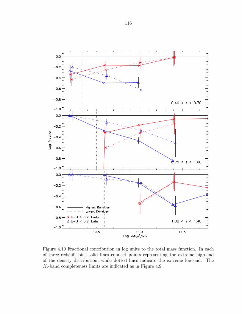
observations are discussed in the conclusions presented in Chapter 7.
16
1.2.4 A Direct Study of the Role of Merging
The hierarchical framework in which galaxies form in dark matter halos and grow by
merging with galaxies hosted in other halos was introduced in §1.1. This theoretical
picture underlies the most advanced semi-analytic (e.g., Cole et al. 2000; Somerville
et al. 2001; Croton et al. 2005; Bower et al. 2005) and numerical (e.g., Nagamine et al.
2004; Springel et al. 2005c) models of galaxy formation today, successfully reproduc-
ing a number of observations including the total stellar mass function, clustering
properties, and the bimodality of galaxies. As discussed previously, late-time (z <∼ 1)
merging is one of the key drivers of evolution in this framework. Not only is it the
means by which galaxies assemble, it is also implicated in the morphological transfor-
mation (e.g., Barnes & Hernquist 1991; Springel et al. 2005a) discussed in Chapter 3
as well as the quenching of star formation (e.g., De Lucia et al. 2005; Hopkins et al.
2005a) described in Chapter 4.
Directly testing and quantifying the role of merging in galaxy evolution remains
a challenging endeavor, however. The problem is, first, how to identify an active
merger and, second, determining the timescale on which the merger proceeds. There
are generally two approaches, and both involve significant uncertainties. First, utiliz-
ing HST one can search for disturbed morphologies suggestive of ongoing interactions
(e.g., Driver et al. 1998; Le Fevre et al. 2000; Conselice et al. 2003; Lotz et al. 2006).
This technique suffers from contamination from non-merging but still irregular sys-
tems, uncertainties in how long the disturbed morphology lasts, and the inability
to distinguish major from minor mergers. The second approach is to count pairs of
nearby galaxies that are assumed to be on the verge of merging (e.g., Patton et al.
1997, 2000; Le Fevre et al. 2000; Lin et al. 2004). Here, contamination from fore-
ground and background sources and, again, uncertainties in the merger timescale pose
significant challenges.
On top of these hurdles, previous studies of the merger rate have relied on optical
diagnostics to probe what is inherently a mass assembly process. In Chapter 5 I
discuss work on the first attempt to constrain the merger rate in terms of stellar
17
mass, allowing this important process to be understood in the context of the mass-
dependent studies presented in Chapters 3 and 4. As reported in Bundy et al. (2004),
this work demonstrates a bias toward higher merger rates in optical observations
compared to the infrared and presents the first estimate of the stellar mass accretion
rate due to merging since z ∼ 1. Extensions of this work are underway and described
in Chapter 7.
1.2.5 Relating Stellar Mass to Dark Matter through Disk
Rotation Curves
The work introduced in the previous sections exploits near-IR stellar mass estimates
to investigate how galaxies assemble and evolve over the interval 0 < z < 1.5. Stellar
mass studies are valuable not only because they provide a census of the stars generated
by the global SFR (see Dickinson et al. 2003) but also because they offer a proxy for
the total mass of a galaxy. It is therefore critical to verify and test the limits of this
relationship between stellar mass and total mass. Clarifying this link also provides
a way of probing the behavior of dark matter, which, under the assumption that it
interacts only through gravity, is more easily understood theoretically compared to
the complex hydrodynamic processes that take place in the luminous component of
galaxies.
Chapter 6 presents work on one of the first attempts to establish the connec-
tion between stellar and dark matter in the context of field galaxy studies. Using
a sample of spiral galaxies with redshifts out to z = 1.2, total masses inferred from
Keck rotation curves were compared to stellar mass estimates gleaned from K-band
photometry. The work presented here is reported by Chris Conselice in Conselice
et al. (2005). My role in the project was assembling the various disparate observa-
tions taken on numerous telescopes over several years, providing the analysis of stellar
masses and the Tully-Fisher relations, and examining our results in terms of specific
models of disk formation (van den Bosch 2002).
Our initial results in this program show a clear trend between stellar mass and
18
total halo mass in this sample with no detected evolution out to z ∼ 1, although our
observations involve significant uncertainties. We present the first measurement of the
high-z stellar mass Tully-Fisher relation, relating stellar mass to maximum rotational
velocity, Vmax, and show how the observations are consistent with the hierarchical
assembly of galaxies in which the mass in baryons and dark matter grows together.
Considering the limitations in the way the sample was selected and the spectroscopic
data quality, we have begun a much more ambitious project using DEIMOS in the
GOODS fields to obtain 8–10 hour rotation curves for a carefully selected sample of
∼120 disk galaxies. This project is described in more detail in Chapter 7.
19
Chapter 2
The Infrared Survey at Palomar:
Observations and Methods for
Determining Stellar Masses
In this chapter I describe an extensive infrared imaging survey I conducted at Palo-
mar Observatory that serves as the core observational component of my thesis. I
discuss the strategy adopted in this survey, its relationship to the DEEP2 Galaxy
Redshift Survey, and the observations as well as photometric analysis. This chapter
also provides details on the method I developed for utilizing infrared observations
to estimate the stellar mass of galaxies. This crucial tool is used in all of the work
presented in this thesis.
2.1 Motivation for the Survey
Over 15 years ago, the advent of new infrared detectors on large telescopes provided
the opportunity to conduct the first galaxy surveys that took advantage of the small
k-corrections (e.g., Kauffmann & Charlot 1998) and relatively low dust extinction in
the near-IR. Because of the small detector area of infrared detectors available at the
time, these surveys were either very shallow, reaching K <∼ 13–17 over 0.2–2 deg2
(e.g., Glazebrook et al. 1991; Mobasher et al. 1993; Glazebrook et al. 1994), or deep
but narrow, reaching K <∼ 21–24 over ∼100 arcmin2 (e.g., Gardner et al. 1993; Cowie
et al. 1994; Djorgovski et al. 1995; McLeod et al. 1995; Saracco et al. 1997). Early
20
science results focused on using K-band number counts to help constrain cosmological
parameters (e.g., Djorgovski et al. 1995) and unravel key aspects of galaxy evolution
(e.g., Broadhurst et al. 1992).
As it became increasingly possible to combine infrared observations with spec-
troscopic redshifts and multi-band optical photometry (e.g., Cowie et al. 1996), the
utility of near-IR luminosities as a stellar mass estimator became apparent (Kauff-
mann & Charlot 1998; Brinchmann & Ellis 2000). Compared to dynamical mass
estimates—which can be derived from spectroscopy for only certain types of galax-
ies (e.g., Vogt et al. 1996; Jorgensen et al. 1996)—infrared mass estimates are a less
expensive proxy (in terms of telescope time) for galaxy mass and can be more easily
measured for entire samples, regardless of type.
Both narrow and wide-field infrared studies began exploiting this capability. The
work by Dickinson et al. (2003) perhaps represents the culmination of near-IR pencil-
beam studies. Using stellar mass estimates based primarily on deep HST/NICMOS
imaging in the Hubble Deep Field–North (HDF–N) region (only 5.0 arcmin2), Dick-
inson et al. (2003) were able to characterize the evolution in the global stellar mass
density over 0 < z < 3 for the first time. In the case of wide-area near-IR surveys
capable of producing statistical samples at z <∼ 1, it has only recently been possible
to improve significantly upon work such as that by Brinchmann & Ellis (2000). They
used a sample of 321 field galaxies imaged in the K-band and the optical with HST
(WFPC2) to show how, since z ∼ 1, the global mass density of various morphological
populations evolves. Examining this global evolution as a function of mass, i.e. mea-
suring the evolving galaxy stellar mass function, requires larger samples, however.
By 2002, when the Palomar survey began, there were two key efforts just finishing
that were motivated in large part by charting the galaxy stellar mass function. The
Munich Near-Infrared Cluster Survey (MUNICS, Drory et al. 2001) began on the
Omega-Prime instrument (6.75× 6.75 arcmin2) at the 3.5m Calar Alto Telescope in
1996. The final MUNICS sample contains 5000 galaxies spread over ≈1 deg2 to a
depth of K <∼ 18.7 (Vega). It consists of primarily (≈90%) photometric redshifts.
Complimentary to MUNICS, the K20 Survey (Cimatti et al. 2002), which began in
21
Figure 2.1 Comparison of the depth and coverage of a number of near-IR sur-veys. Filled symbols denote surveys with significant spectroscopic follow-up: Palo-mar/DEEP2 shows the three nested surveys described in this chapter (§2.2.2); BundyGOODS refers to Chapter 3 and Bundy et al. (2005a); Cohen refers to the CaltechFaint Galaxy Redshift Survey (see Hogg et al. 2000; Cohen 2002); K20 is presentedin Cimatti et al. (2002); Cowie96 is the Hawaii Deep Field work (Cowie et al. 1996);and HDF refers to the work by Papovich et al. (2001) and Dickinson et al. (2003).Open symbols represent surveys without spectroscopic follow-up: MUNICS refers tothe survey presented in Drory et al. (2001); UKIDSS UDS is the deepest compo-nent of the UKIRT Infrared Deep Sky Survey, which finished K-band imaging in late2005; Saracco97 A and B are subsamples of the ESO K’-band Survey (Saracco et al.1997); McCracken00 A and B are subsamples of the work discussed in McCrackenet al. (2000); and FIRES is the Faint IR Extragalactic Survey (Labbe et al. 2003). Itshould be noted that the UKIDSS Deep Extragalactic Survey (DES, their “medium”depth effort) is 36% complete (as of February 2006) in its K-band imaging goal ofK = 21 over 35 deg2—this part of parameter space is literally “off the chart” on thefigure above.
22
1999 on the ESO VLT, has surveyed about 550 galaxies—most (92%) with spectro-
scopic redshifts—down to K < 20 over an area of 52 arcmin2.
While the MUNICS and K20 programs represent significant progress in wide near-
IR surveys and led to many results (e.g., Fontana et al. 2004; Drory et al. 2004a), each
suffers from important limitations. MUNICS is too shallow to reliably probe below the
characteristic mass,M∗, at z ∼ 1, and its reliance on photometric redshifts introduces
significant uncertainties in stellar mass estimates (see §2.4). The K20 Survey, on the
other hand, suffers from substantial random errors and cosmic variance because of its
small size, preventing detailed studies of sub-populations within the primary sample
and reducing the statistical significance of the results. The infrared survey at Palomar
was designed to address these limitations.
The primary goals of the survey were to fully characterize the evolving stellar
mass function and chart the assembly history of the galaxy population as a function
of various physical parameters. These goals set clear specifications for the survey.
To mitigate cosmic variance, for example, the surveyed area had to be at least 1.0
deg2. Furthermore, building a statistically complete sample that would be robust
to various cuts and sensitive to evolutionary trends required ∼10,000 galaxies with
spectroscopic redshifts out to z ∼ 1. Finally, to probe the mass function below M∗,
we set a target depth of K = 20 (Vega), with a good fraction of the sample aimed
at K >∼ 21 to detect even fainter galaxies and test for incompleteness. A comparison
of the depth and area covered by the Palomar survey to a selection of other near-IR
surveys is made in Figure 2.1.
The Wide Field Infrared Camera (WIRC, Wilson et al. 2003), successfully com-
missioned on the 5m Hale Telescope at Palomar Observatory in 2002, provided the
large field of view (8.6×8.6 arcmin2) and sensitivity needed for achieving these goals.
At the same time, the DEEP2 Galaxy Redshift Survey (Davis et al. 2003) had be-
gun its second year, delivering what would be an unprecedented spectroscopic sample
at z ∼ 1—the perfect data set for subsequent follow-up imaging with WIRC. After
several nights of testing in late 2002, we began our infrared campaign as a Palomar
“Large Program” in 2003a and completed it two and a half years later.
The layout and much of the strategy behind the Palomar survey was shaped by the
nature and progress of the DEEP2 Galaxy Redshift Survey (Davis et al. 2003). More
details about the DEEP2 sample and its contribution to the major scientific results
of this thesis are presented in Chapter 4, but I present some of the key features of
DEEP2 here.
The DEEP2 survey is comprised of four independent regions covering a total area
of more than 3 square degrees. The properties of the four fields are summarized in
Table 2.1. The DEEP2 redshift targets were selected based on BRI colors determined
from observations with the CFHT 12k camera, which has a field of view of 0.70 × 0.47
(see Coil et al. 2004). DEEP2 Fields 2–4 are composed of three contiguous CFHT
pointings, oriented from east-to-west. The Extended Groth Strip (EGS, also known
as Field 1) has a different geometry, encompassing and extending the original Groth
Strip Survey (Groth et al. 1994) to a swath of sky 16′ wide by 1.5 long and oriented at
a ∼45 position angle. This geometry required four tiered CFHT pointings because
the 12k camera cannot be rotated.
With the four target fields defined in this way, the DEEP2 team concentrated
first on observing the central CFHT pointing in Fields 2–4. In the EGS, DEEP2
observations began at the southern end of the field and progressed upward. For all
four fields, we coordinated the Palomar Ks-band observations to track the progress of
24
Figure 2.2 WIRC pointing layout and Ks-band depth in the EGS. The region imagedby HST/ACS is indicated by the central rectangle.
25
Figure 2.3 WIRC pointing layout and Ks-band depth in Fields 2–4. The shadingdepth is the same as in Figure 2.2.
26
DEEP2. Palomar Ks-band coverage is complete in the central third of Fields 3 and 4.
In Field 2, 80% of the central CFHT pointing was surveyed and the coverage in the
EGS is 100%. The EGS was considered the highest priority field in view of the many
ancillary observations—including HST, Spitzer, and X-ray imaging—obtained there.
The final Palomar Survey covers 1.6 square degrees, with Fields 2–4 accounting for
0.9 square degrees, and the EGS accounting for 0.7. Coverage maps for each of the
four regions are shown in Figures 2.2 and 2.3.
2.2.2 Depth of Ks-band Coverage
A tiered approach was adopted to maximize the depth and coverage of the survey
while addressing the typical weather patterns at Palomar. A base target depth of
Ks = 20.0 (Vega or 21.8 in AB magnitudes) was used for all pointings. At z ∼ 1,
a galaxy with Ks = 20 roughly corresponds to a stellar mass of 1010 M⊙, which is
about one order of magnitude less than the characteristic mass, M∗. The Ks = 20
limit was also chosen because it is achievable in 1–2 hours of integration time in
average to mediocre conditions (determined mainly from the seeing FWHM which is
≈1′′ in the Ks-band in average Palomar conditions). When conditions were superior,
with seeing of 0.′′6–0.′′9 (this occurred only about ∼15% of the time, unfortunately),
we concentrated on select fields with the goal of reaching Ks = 21 (Vega), enabling
detections of galaxies with stellar masses of ≈5 ×10⁹ M⊙ at z ∼ 1. The magnitude
depth quoted here is defined as the 5σ detection limit in an aperture with a diameter
equal to the seeing FWHM. Tests showed this depth estimate to be comparable to
the 80% completeness limit determined from Monte Carlo simulations using inserted
fake sources (see 2.3.1).
This strategy effectively combines several surveys of different depths into one (see
the “Palomar/DEEP2” data points in Figure 2.1). Our shallowest component covers
1.5 square degrees to Ks > 20.0. This was the base goal for the depth in all of
the observations. Nested within this area is a deeper component covering 0.8 square
degrees to Ks > 20.5. And within this component, 0.14 square degrees reach Ks > 21
27
Figure 2.4 This figure illustrates the redshift detection rate in each of the four fields.The dotted histograms show the RAB number counts for galaxies with successfulDEEP2 redshifts. The shaded histogram illustrates the fraction of these galaxies thathave Ks-band detections. The EGS field is clearly the deepest in terms of detectedDEEP2 sources.
28
(most of the deepest pointings are in the central portion of the EGS). This tiered
approach enables one to generate comparable samples across a broad redshift range
by constructing redshift intervals that balance the size of the cosmic volume sampled
with the stellar mass limit probed (see 4.2.3).
The depth of the observations also determines the fraction of DEEP2 redshift
galaxies that are detected in the Ks-band. This fraction ranges from ≈65% for Ks-
band depths near Ks = 20 to ≈90% for Ks = 21. The Ks-band depth and redshift
detection rate for each field are illustrated in Figure 2.4.
2.2.3 Mapping Strategy
The field-of-view of WIRC is 8.′7 × 8.′7, and it has a fixed orientation on the sky with
its y-axis aligned North–South. In each of the four fields in the survey, WIRC target
pointings were chosen to cover the full extent of DEEP2 redshift sources and were
tiled to minimize the overlap between adjacent WIRC pointings. The advantage of
this kind of tiling pattern—as opposed to one with overlap between images—is that
it maximizes the area covered. The down side is that each pointing has to be photo-
calibrated independently, leading to the possibility of slight zeropoint offsets from
one pointing to the next. However, because of the relatively low number density of
bright K-band sources, self-calibration between overlapping pointings would require
shared regions that are at least 25% of the WIRC field of view, significantly reducing
the total survey area. In addition, it is difficult in practice to make sure that each
set of exposures, taken at a given pointing over different nights, is perfectly aligned
with previous observations at the same position. This is due to occasional pointing
problems on the 200 inch Hale Telescope as well as glitches in the dither script, both
of which can lead to spatial offsets of tens of arcseconds, making the alignment of
adjacent mosaics more difficult.
The tiling patterns are straightforward in the case of Fields 2–4 because these rect-
angular areas are also aligned along the N–S/E–W axes (see Figure 2.3). The long and
narrow EGS region is tilted at a ∼45 position angle. To fully cover the spectroscopic
29
observations in the E–W direction required rows of three WIRC pointings. The N–S
direction required about 12 different positions, so, in total, 35 WIRC pointings were
used to map the EGS in the Ks-band (Figure 2.2). Roughly two-thirds of the WIRC
pointings in the EGS contain regions of sky without DEEP2 spectroscopic targets.
These perimeter pointings were given less priority than the central WIRC positions
for this reason, so the deepest EGS exposures (Ks >∼ 21) were taken in positions along
the center of the EGS. In addition, there is, in general, better Ks-band data in the
southern portion of EGS because DEEP2 redshifts were first acquired there (as of
the completion of this work, the northern 20% of the EGS DEEP2 observations were
not complete). Finally, deep Ks-band imaging was extended northward to include
the region of the EGS covered by HST/ACS observations in 2004 (see Figure 2.2).
The mapping mode on a given night was chosen based on the observing conditions.
In excellent conditions, the exposure time at a given WIRC position could add up
to several hours. In average conditions, 1–2 hours was spent integrating at a given
position before moving on to the next pointing. The choice of which WIRC pointing
in a given field to expose on was determined by the data already available in that
field as well as the conditions at the time so that each new observation would provide
the maximum scientific return for the survey.
With most of the shallow (Ks >∼ 20) component of the survey completed, J-band
observations were obtained in the case of average conditions during the last year of
the survey. In Fields 3 and 4, J-band imaging to J <∼ 22 (Vega) was obtained for
80% and 100% of each field, respectively. No J-band data was taken in Field 2, and
in the EGS we carried out deep J-band imaging (J <∼ 23) along the central 9 WIRC
pointings. These positions were chosen because they are coincident with the deepest
Ks-band data and overlap with the HST/ACS region. The same WIRC positions and
tiling patterns used in the Ks-band were also used in the J-band.
30
Figure 2.5 The WIRC Ks filter response (solid line) compared the Kitt Peak IRIMK-band filter (dashed line) and a normalized blackbody spectrum at T = 300 K(dotted line).
2.3 Observations and Data Reduction
Near-IR observations from the ground are background-limited due to the thermal
radiation from the atmosphere.1 The Ks filter is designed with a sharper red cut-
off compared to the K filter to help limit the background contribution (see Figure
2.5), but with sky background levels of Ks ∼13 mag/arcsec2 (typical for Palomar
Observatory), short integrations are required to prevent detector saturation. For
WIRC’s 2048 × 2048 Hawaii-II HgCdTe detector (additional details on the detector
are provided in Table 2.2), our tests confirmed that the response became nonlinear
at ∼25,000 adu. This restricts Ks-band integration times to 20 seconds in conditions
with T ∼ 20C, 30 seconds with T ∼ 10C, and 40 seconds with T ∼ 0C. Before
and after each exposure, 3.25 seconds are required to read out the array, so choosing
the longest exposure time allowed by the conditions helps increase the efficiency of
1Wein’s Law gives λpeak ∼ 10µm for a blackbody at T = 300 K, roughly the temperature of theatmosphere.
31
Table 2.2. WIRC Characteristics
Hawaii-II HgCdTe Detector
Position on 200 inch Prime Focus, f/3.3Field of view 8.7 arcmin2
Sky background levels in the near-IR vary on scales of several minutes (K. Matthews,
priv. communication). To remove these fluctuations, individual Ks-band exposures
at a given WIRC pointing and dither position were taken with an integration time
of 2 minutes before moving to the next dither position. By changing the number
of coadds per position—6 coadds × 20 seconds (T ∼ 20C), 4 coadds × 30 seconds
(T ∼ 10C), or 3 coadds × 40 seconds (T ∼ 0C)—the 2 minute integration time was
maintained under all conditions, making it easier to stack images taken on different
nights. The vast majority of observations were obtained in the 4× 30 second mode.
In all observations, 2 minute exposures were dithered over a 3 × 3 grid (Figure
2.6). The grid point spacing was chosen to be 7′′ to insure accurate photometry
for target galaxies as large as ∼3′′ while minimizing the slew time between dither
positions. Because adjacent exposures contribute significantly to the flat fielding of
a given frame (see below), the sequence for slewing to each point in the grid was
chosen to maximize the dithered offset between frames (the sequence is numbered in
Figure 2.6). This 9-point sequence was typically repeated 3 times at a given pointing
so that the full dither pattern contained 27 positions and a total integration time
of 54 minutes. A random spatial offset, typically ∼1.′′5, was applied to each of the
27 positions. This prevented direct overlap in the 54-minute observation set and
improved the final image quality. The main sources of overhead were reading out the
detector and slewing to the next dither position. With the most common set-up of
32
Figure 2.6 The 3 × 3 dither pattern used in the WIRC observations. The numbersindicate the order in which the pattern was executed. A random spatial offset of ∼1.′′5was applied at each position.
4 × 30 sec exposures, a full set of 27 frames and 54 minutes on sky corresponds to
about 70 minutes of clock time, giving an efficiency of 77%.
Camera control and data taking were carried out using a dual-processor “Linux
box.” A second, identical machine was purchased in early 2003 as a back-up and
was also configured to “grab” incoming raw data and store it on a separate hard
drive, independent from the control computer. Most data reduction and analysis was
performed on this second machine to help prevent crashes of the control computer. It
was possible, however, to examine subtracted “first-look” images on the data-taking
machine, as this process does not require significant computation. As illustrated in
Figure 2.7, the dominant sky background and flat-field pattern which obscures most
astronomical sources in raw Ks-band frames can be removed simply by subtracting
two images from an observing sequence. With the background removed and sources
now visible, the result can be easily inspected to determine the seeing and focus
accuracy by measuring the profile shape of stars in the field of view. Based on such
measurements, it was often possible to adjust the focus “on the fly” without significant
interruption to the observing sequence.
33
-
=
Raw Frame 1 Raw Frame 2
Subtracted Frame
(spatial offset)
Figure 2.7 Example of subtracting two raw WIRC frames to obtain a “first look”image. The two raw images shown at the top are part of a set of 4 × 30 secondobservations taken on October 20, 2005 in average conditions with seeing FWHMof 1.′′1. The dominant background and flat-field pattern common to both images isapparent and obscures all but the brightest astronomical sources in the raw frames.Pairs of positive and negative sources are easily seen in the subtracted frame, however.Their separation of ∼7′′ reflects the dither offset between the two frames.
34
In addition to generating first-look subtracted frames, a full data reduction pipeline
I developed specifically for WIRC could be run on the secondary computer while ob-
servations were being taken. Despite the relatively large file sizes (each coadded
WIRC exposure is ∼16 MB), a set of 27 exposures (54 minutes on sky) could be fully
reduced in just over 20 minutes, allowing for near real-time inspection of the final
image quality and observing conditions.
The image reduction pipeline first creates a “running sky flat” for a given science
frame by (median) averaging together 3 adjacent frames taken before and 3 taken
after the science frame (see Figure 2.8). Each science frame is then divided by its
corresponding sky flat, which tracks the detector sensitivity and illumination pattern
of the telescope during the course of the observations. Experimentation showed that
neither dome flats nor twilight flats provide an adequate flat field for WIRC, presum-
ably because of different illumination patterns and stray light. Variations in the night
sky background (due to clouds, as an extreme example) also affect the illumination
pattern. This means that sky flats created at one time of night are not suitable for
reducing data taken later that night, let alone data taken on different observing runs.
With each science frame divided by a median sky flat, stars and galaxies are easily
detected. By cross-correlating the science frames, the spatial offset between them in
pixels can be determined. The telescope pointing position (which is stored in the
image header) is used as an initial guess for these offsets, but is not accurate enough
to align the science frames. At this point in the reduction pipeline, an object mask is
made based on the location of bright sources in the first frame. Knowing the spatial
offsets between each frame, this mask is applied to the creation of new sky flats in
which objects on adjacent frames are masked out before these frames are averaged
together (Figure 2.8). This provides significantly cleaner sky-flat fields and improves
the final, coadded image quality. After this second pass of improved flat fielding, the
science frames are aligned and stacked into the final mosaic. In practice, the pipeline
works with sets of 12 frames at a time to prevent the memory requirements on the
processing computer from becoming unmanageable.
The pipeline was tested extensively and functions without need for human inter-
35
Figure 2.8 Schematic diagram outlining the steps in the double-pass WIRC reductionpipeline. For illustration purposes, the frames shown above are from the SE quadrantof the detector and only 3 frames are shown, whereas in practice, sky flats are createdfrom 6 frames.
36
Figure 2.9 An example of the image quality obtained from a deep (Ks ≈ 21, Vega)mosaic in Field 4 with DEEP2 sources circled and redshifts indicated.
action about 90% of the time when observing conditions are good. One common
problem it does not address is the occasional satellite trail across an image frame. I
found that these trails, even in one image, will propagate into the final mosaic and
so I simply removed frames with satellite trails from the reduction set. When there
are clouds present, flat fielding becomes problematic and the cross-correlation routine
can fail. In these cases, the pipeline will ask for help in choosing the correct align-
ment. It can also be executed in a more interactive mode in which the user can use
the mouse to select common objects in each frame, the positions of which are then
used to align the observations and make the final mosaic. The reduction pipeline was
made publicly available and has been used by other WIRC observers.
At a given pointing, individual 54-minute mosaics were often obtained on different
nights and so may vary in terms of seeing, sky background levels, and transparency.
Most Ks-band pointings consist of more than two independently combined mosaics,
with the deepest pointings comprising as many as 6 independent mosaics. Mosaic
coaddition was performed using an algorithm that optimizes the depth of the final
37
image by applying weights based on the seeing, background, and transparency of the
constituent mosaics. Following Labbe et al. (2003), the weight of mosaic i is given by
wi ∝ (scalei × vari × s2i )−1, (2.1)
where scalei is the flux scale factor and accounts for transparency, vari is the variance,
and si is the seeing FWHM. The final seeing FWHM in the Ks-band data ranges from
0.′′8 to 1.′′2 and is typically 1.′′0. An example of the data quality in a final Ks-band
mosaic is shown in Figure 2.9.
2.3.1 Photometry and Catalogs
Photometric calibration was carried out separately in each field by observing Persson
near-IR standards (Persson et al. 1998) and taking short, 5-minute calibration images
at each WIRC position during photometric conditions. These short integrations are
sufficient for detecting objects at Ks <∼ 18, and the number density of strongly de-
tected sources (about 10 with 12 < Ks < 16 per image) enables zeropoint calibration
for the final mosaics that is typically good to 0.02 mags. This is superior to calibrat-
ing with 2MASS, which has a brighter detection limit, leading to fewer sources in
common with the final WIRC images and zeropoint uncertainties of ∼0.06 mags (and
sometimes more). The use of 2MASS is also complicated by the fact that bright stars
(Ks <∼ 12) often saturate in the WIRC frames and cannot be used for photometric
calibration. I note that the DEEP2 CFHT B and I photometry is calibrated with
respect to the CFHT R-band by comparing to the stellar locus in color-color space
(Coil et al. 2004). A similar technique could in theory work for the K-band, but the
WIRC field-of-view does not contain enough stars (for fields at high galactic latitude)
to sample the stellar locus sufficiently. This technique will be possible in the future
with larger format near-IR cameras.
The final WIRC mosaics were registered to the DEEP2 astrometric system (see
Coil et al. 2004) using bright stars from the CFHT R-selected catalog. The typical
root mean square (rms) variation in the astrometric solutions was 0.1′′. In the EGS,
38
WIRC images were also registered to the 2MASS astrometry to allow for comparisons
to Spitzer Space Telescope IRAC data, which uses the 2MASS system. Each of the
final Ks-band mosaics were inspected visually, and a mask was made to exclude the
low signal-to-noise perimeter that results from stacking dithered images. Only ∼8%
of the area in the final mosaic was typically masked out.
With the final Ks-band images prepared in this way, we used SExtractor (Bertin
& Arnouts 1996) to detect and measure Ks-band sources. In addition to the total
magnitude (for which we use theMAG AUTO output—we do not adjust this Kron-
like magnitude to account for missing light in extended sources), we also measured
aperture photometry in 2′′, 3′′, 4′′, and 5′′ diameters (later experimentation with SED
modeling and color-color diagrams indicated that the 2′′ diameter aperture colors
were the most precise). We combined the resulting SExtractor catalog output for
each Ks-band image in a given field to create K-selected catalogs.
To determine the corresponding magnitudes of Ks-band sources in the CFHT BRI
and Palomar J-band images, we applied the IDL photometry procedure, APER,
placing apertures with the same set of diameters at sky positions determined by
the Ks-band detections. About 25% of the Ks-band sources do not have optical
counterparts in the CFHT optical data. Source pairs from overlapping images with
measured separations less than 1.′′0 were considered duplicates, and the source with
the poorer signal-to-noise was removed from the final catalog.
Photometric errors and the Ks-band detection limit of each image were estimated
by randomly inserting fake sources of known magnitude into each Ks-band image
and recovering them with the same detection parameters used for real objects. The
inserted objects were given Gaussian profiles with a FWHM of 1.′′3 to approximate
the shape of slightly extended, distant galaxies. We define the detection limit as the
magnitude at which more than 80% of the simulated sources are detected. Robust
photometric errors based on simulations involving thousands of fake sources were also
determined for the BRI and J-band data. These errors are used to determine the
uncertainty of the stellar masses and in the determination of photometric redshifts,
where required.
39
For each of the four fields, FITS table catalogs were made that include information
on each K-detected source in that field. This includes the BRIJK photometry, es-
timated magnitude uncertainties, positions, the corresponding Ks-band image depth,
DEEP2 spectroscopic redshifts (where available), photometric redshifts (see §4.2.4),
and stellar mass estimates (described below). These catalogs have been made avail-
able to the DEEP2 team which has used them extensively, and they will become
publicly available as the DEEP2 survey is released to the public, beginning in 2007.
2.4 Estimating Stellar Mass
One of the primary motivations for the Palomar near-IR survey was the ability to use
Ks-band observations combined with spectroscopic redshifts to estimate the stellar
mass of survey galaxies. Because K-band stellarM∗/L ratios are relatively insensitive
to the detailed makeup of stellar populations, K-band luminosities alone provide stel-
lar mass estimates that are uncertain by factors of 5–7 (Brinchmann 1999). However,
for samples with known spectroscopic redshifts, optical-infrared color information can
further constrain the stellar population and M∗/L ratio so as to reduce this uncer-
tainty to a factor of 2–3. The basic technique relies on accurate luminosity distances
from spectroscopic redshifts to determine the near-IR (K-band) luminosity of sample
galaxies. With a M∗/LK constrained by comparisons of the galaxy SED to model
expectations, the luminosity can be multiplied by the mass-to-light ratio to derive
an estimate for the stellar mass (LK ×M∗/LK = M∗) with relatively high precision.
Building on the precepts discussed in Brinchmann & Ellis (2000) and Kauffmann
et al. (2003a), I have developed my own Bayesian code for estimating stellar mass
and describe it below.
The code uses spectroscopic redshifts and multi-band optical through near-IR col-
ors (typically BRIK) to compare the observed SED of a sample galaxy to a grid of
13440 synthetic SEDs compiled from the stellar population synthesis package devel-
oped by Bruzual & Charlot (2003). The templates in this grid represent the assumed
priors in this Bayesian technique and span 4 dimensions in parameter space: star for-
40
mation history (τ), age, metallicity, and dust content. The star formation histories
are parametrized as exponentials (SFR ∝ e− tτ ), with 35 τ values selected randomly
Z = [0.0001, 0.0004, 0.004, 0.008, 0.02 (Z⊙), 0.05].
Finally, the dust content is parametrized by varying τV , the total effective V -band
optical depth affecting stars younger than 107 yr, while setting the fraction of this
extinction contributed by the ambient ISM to µ = 0.3 (see Bruzual & Charlot 2003).
The values of τV are
τV = [0.0, 0.5, 1, 2].
The values of the parameters listed above were chosen with the goal of fully sampling
the possible range of observations. Comparisons between observed galaxy colors and
model colors verified that the model space defined above is representative, although
the degree to which it reflects real galaxies is an inherent limitation in this technique.
Finally, it is important that the sampling of model parameters be random. Systematic
biases can be introduced in the results by assuming the values of priors are spaced in
a certain way (Sivia 1996).
A unique template spectrum is stored at each grid point and is then compared to
the observed galaxy’s SED after applying the appropriate redshift and transmission
41
functions for each filter band. The probability that the specified model at each grid
point accurately describes the observed SED is given by
P ∝ exp (−χ2
2) with χ2 =
N−1∑i
[(mi −mi+1)model − (mi −mi+1)obs]2σ2i + σ
2i+1
, (2.2)
where i ranges over the observed filters andmi is the measured magnitude in filter i. In
this way, χ2 effectively measures how well the colors of the template spectrum match
the colors of the observed galaxy, modulo the photometric uncertainty (σi). This
relative probability is calculated at each point in the grid, giving a multi-dimensional
probability “cloud” whose size, shape, and position reflects the range of models that
best fit the observations, given their uncertainty.
In addition to the relative probability, the corresponding M∗/LK ratio of each
model in the grid is also tracked and converted into a stellar mass by scaling the
total Ks-band luminosity of each model (roughly equal to LK⊙ for the Bruzual &
Charlot (2003) models) to the galaxy’s observed LK . The probabilities are then
summed (marginalized) across the grid, renormalized, and binned by model stellar
mass. This gives a stellar mass probability distribution for each sample galaxy. We
use the median of the distribution as the best estimate. Several examples taken from
Bundy et al. (2005a) are shown in Figure 2.10.
The stellar mass measured in this way is robust to degeneracies in the model,
such as those between age and metallicity. Although these degeneracies can produce
bimodal probability distributions (see Figure 2.10), even in these cases, the typical
width of the distribution gives uncertainties from the model fitting alone of 0.1–0.2
dex. For about 2–3% of the SED fits, the minimum χ2 values are significantly greater
than 1.0. For these more poorly-constrained objects, we add an additional 0.2 dex
in quadrature to the final mass uncertainty. Although in principle the best fitting
model also provides estimates of the age, metallicity, star formation history, and dust
content of a sample galaxy, these quantities are much more affected by degeneracies
and are poorly constrained compared to the stellar mass.
42
Figure 2.10 Examples of the best-fitting model spectra and the resulting stellar massprobability distribution as determined by the stellar mass code (from Bundy et al.2005a). The photometry points are plotted and final mass indicated. The dashedlines denote the 68% confidence intervals in the derived stellar mass.
43
Photometric errors enter the analysis by determining how well the template SEDs
can be constrained by the data. Larger photometric uncertainties “smear out” the
portion of the model grid that fits an observed galaxy with high probability. This is
reflected in a wider stellar mass probability distribution. Additional uncertainties in
the Ks-band luminosity (from errors in the observed total Ks-band magnitude) lead
to final stellar mass estimates that are typically good to 0.2–0.3 dex. The largest
systematic source of uncertainty comes from the assumed IMF, in this case that
proposed by Chabrier (2003). The stellar masses we derive using this IMF can be
converted to Salpeter by adding 0.3 dex.
2.4.1 Optical Masses, Photo-z’s, and Other Caveats
The combination of extensive spectroscopic redshifts and K-band photometry makes
the DEEP2/Palomar survey an ideal and unique data set for tracing the stellar mass
evolution of galaxies. Other groups have attempted to estimate stellar masses without
this important combination, lacking spectroscopy (e.g., Drory et al. 2004a), near-IR
data (e.g. COMBO17), or both (e.g., Gwyn et al. 2005). I discuss some concerns
about these efforts as well as general caveats about stellar mass estimates below.
Spectroscopic redshifts not only precisely locate galaxies in space and time but
enable the reliable determination of restframe quantities such as color and luminosity
which are critical for accurate comparisons to stellar population templates and the
ability to measure luminosity and convert to stellar mass. The additional stellar
mass uncertainty resulting from the use of typical photo-z’s is illustrated in Figure
2.11, taken from Bundy et al. (2005a). In this experiment we measure photometric
redshifts for galaxies that already have secure spectroscopic redshifts and use these
photometric redshifts to determine a second set of stellar mass estimates. Figure
2.11 shows the difference in stellar mass for the same galaxies when photometric
redshifts are used instead of spectroscopic redshifts, plotted as a function of their
spectroscopic redshift. Individual mass estimates become less certain, and there are
several catastrophic outliers with stellar masses that differ by an order of magnitude.
44
Figure 2.11 Difference in estimated stellar mass for our spectroscopic sample whenphoto-z’s are used instead of spec-z’s. The shaded region shows the expected standarddeviation resulting from variations in the luminosity distance due to photo-z error.
The shaded region shows the standard deviation in stellar mass error based on a
Monte Carlo simulation of 20,000 galaxies in which simulated redshifts were drawn
from the observed photometric redshift error distribution (σ[∆z/(1+z)] = 0.12). The
simulation includes only the primary effect on the luminosity distance. The shaded
region accounts for both the rms uncertainty and the effect of catastrophic photo-z
failures since both are included in the measurement of σ[∆z/(1 + z)].
Figure 2.11 shows a systematic offset such that most of the dramatic outliers tend
to have lower masses when photometric redshifts are used than when spectroscopic
redshifts are used. This trend is a common result of photo-z codes based on priors,
which, as discussed in §3.2.3, often assign outliers lower photo-z measurements as
compared to their spectroscopic values. The smaller luminosity distance that results
from the photo-z underestimate leads to stellar masses that are also underestimated.
The importance of near-IR observations was discussed by Kauffmann & Charlot
(1998) and first exploited by Brinchmann & Ellis (2000) who demonstrate that near-
infrared and especially K-band photometry traces the bulk of the established stellar
45
Figure 2.12 Uncertainties present in optical stellar mass estimates. The left-handplot shows the difference between stellar masses estimated with BRI photometry andthose with K-band included, based on a random sample drawn from the EGS. At allredshifts there are significant discrepancies in the optical masses. The range of errorsincreases beyond z = 0.75 (dotted line). This is also apparent in the uncertainties ofthe optical masses plotted in the middle diagram. The IR masses maintain relativelylow uncertainties at all redshifts in the DEEP2 sample.
populations and enables reliable stellar mass estimates for z <∼ 1.5. With the addition
of SED fitting from multi-band optical photometry, the final uncertainty in such
estimates can be reduced to factors of∼2 based onK-band observations out to z ≈ 1.5
(Brinchmann & Ellis 2000). The importance of K-band observations is highlighted
in Figure 2.12. At all redshifts the optical masses derived from BRI photometry
exhibit significant errors, some approaching an order of magnitude discrepancy. This
is especially a problem for galaxies with z > 0.75, where the I-band filter begins
sampling the restframe SED blueward of the 4000 angstrom break. As shown in
the middle plot of Figure 2.12, estimated uncertainties from optical mass estimates
become even less secure as the redshift increases and increasingly bluer portions of
the restframe SED are shifted into the reddest filter bands. Thus, a comparison to
Figure 2.11 shows that the combined lack of K-band photometry and spectroscopic
redshifts leads to stellar mass errors greater than factors of 5–10 with catastrophic
failures off by nearly two orders of magnitude.
Even with the combination of near-IR and spectroscopic redshifts, stellar mass
46
estimates like those described here suffer inherent uncertainties and are unlikely to
improve much beyond the 50% level even with the best observations. The primary
difficulty lies in accurately modeling the stellar population. The code described in
the previous section uses the simplest simple stellar population (SSP) models, and
while these do a fair job representing the global properties of galaxies, they are lim-
ited in accuracy because they cannot reflect the complex formation history we know
most galaxies undergo. Some authors like Papovich et al. (2001) and Kauffmann
et al. (2003a) have fit observed SEDs with multi-component models. These are typ-
ically used to constrain the maximum allowable stellar mass, but they entail added
complexity and parameters which are difficult to constrain and in most cases do not
improve the final mass estimate.
Furthermore, even templates with precise and accurate star formation histories
suffer from the assumptions that go into them. Comparisons between different models
made by different authors using the same parameters do not always give the same
results (Drory et al. 2004b). There are differences in prescriptions for abundance
ratios, dust extinction, and the contribution of hard-to-model components like AGB
stars, to name a few (see Bruzual & Charlot 2003).
So, while stellar estimates provide a unique and valuable tool for charting galaxy
evolution, their utility and precision only goes so far and is unlikely to be vastly
improved upon in the future. In the work described in the following chapters, I rely
heavily on stellar mass estimates to trace the evolution of galaxies but maintain a
conservative approach when evaluating their precision.
47
Chapter 3
The Mass Assembly Histories of
Galaxies of Various Morphologies
in the GOODS Fields1
We present an analysis of the growth of stellar mass with cosmic time partitioned
according to galaxy morphology. Using a well-defined catalog of 2150 galaxies based,
in part, on archival data in the Great Observatories Origins Deep Survey (GOODS)
fields, we assign morphological types in three broad classes (Ellipticals, Spirals, Pe-
culiar/Irregulars) to a limit of zAB=22.5 and make the resulting catalog publicly
available. Utilizing 893 spectroscopic redshifts, supplemented by 1013 determined
photometrically, we combine optical photometry from the GOODS catalog and deep
Ks-band imaging to assign stellar masses to each galaxy in our sample. We find lit-
tle evolution in the form of the galaxy stellar mass function from z ∼ 1 to z = 0,
especially at the high mass end where our results are most robust. Although the pop-
ulation of massive galaxies is relatively well established at z ∼ 1, its morphological
mix continues to change, with an increasing proportion of early-type galaxies at later
times. By constructing type-dependent stellar mass functions, we show that in each
of three redshift intervals, E/S0’s dominate the higher mass population, while spirals
are favored at lower masses. This transition occurs at a stellar mass of 2–3×10¹⁰
M⊙ at z ∼ 0.3 (similar to local studies), but there is evidence that the relevant mass
scale moves to higher mass at earlier epochs. Such evolution may represent the mor-
1Much of this chapter has been previously published as Bundy et al. (2005a)
48
phological extension of the “downsizing” phenomenon, in which the most massive
galaxies stop forming stars first, with lower mass galaxies becoming quiescent later.
We infer that more massive galaxies evolve into spheroidal systems at earlier times
and that this morphological transformation may only be completed 1–2 Gyr after
the galaxies emerge from their active star forming phase. We discuss several lines of
evidence suggesting that merging may play a key role in generating this pattern of
evolution.
3.1 Introduction
Great progress has been made in recent years in defining the star formation history
of galaxies (Madau et al. 1996; Blain et al. 1999). The combination of statistically
complete redshift surveys (Lilly et al. 1995a; Ellis et al. 1996; Steidel et al. 1999;
Chapman et al. 2003) and various diagnostics of star formation (UV continua, recom-
bination lines, and sub-mm emission) has enabled determinations of the co-moving
star formation (SF) density at various redshifts whose rise and decline around z ≃ 2
points to the epoch when most stars were born (e.g., Rudnick et al. 2003; Bouwens
et al. 2003; Bunker et al. 2004). Many details remain to be resolved, for example
in reconciling different estimators of star formation (e.g., Sullivan et al. 2004) and
the corrections for dust extinction. In addition, recent theoretical work including
both numerical simulations and semi-analytic modeling is in some confusion as to the
expected result (e.g., Baugh et al. 1998; Somerville et al. 2001; Nagamine et al. 2004).
An independent approach to understanding how galaxies form is to conduct a
census of galaxies after their most active phases and to track their growing stellar
masses. The co-moving stellar mass density at a given redshift should represent
the integral of the previously-discussed SF density to that epoch, culminating in
its locally-determined value (Fukugita et al. 1998). Unlike the star formation rate
(SFR), the stellar mass of a galaxy is less transient and can act as a valuable tracer
for evolutionary deductions.
Further insight is gained by tracing the integrated growth in stellar mass of dif-
49
ferent populations. For example, the rapid decline with time in the SF density over
0 < z < 1 (Lilly et al. 1996; Fall et al. 1996) appears to result from the demise of an
abundant population of star forming, irregular galaxies (Glazebrook et al. 1995; Abra-
ham et al. 1996; Brinchmann et al. 1998). By considering the declining stellar mass
density associated with irregular galaxies, Brinchmann & Ellis (2000) suggested that
these sources transform, either by mergers or other means, into the slowly growing
mass identified with regular ellipticals and spirals.
In a complementary fashion, the recent completion of large infrared surveys like
K20 (Cimatti et al. 2002) and MUNICS (Drory et al. 2001) has traced the distribution
in mass of the most massive galaxies out to z ∼ 2 (Fontana et al. 2004; Drory et al.
2004a). These and other studies find a decrease in the overall normalization of the
combined galaxy stellar mass function with redshift. Fontana et al. (2004) find very
little evolution in the shape of the combined mass function out to z ∼ 1. Drory et al.
(2004a), in contrast, argue for a stronger evolution out to z ∼ 1 based on a decrease in
the characteristic mass and steepening of the faint–end slope. The MUNICS survey,
though extensive in size, relies primarily on photometric redshifts and, at K <∼ 18.7
(Vega), probes a limited mass range. The deeper K20 survey, on the other hand,
utilizes primarily spectroscopic redshifts but is much smaller and suffers more from
cosmic variance.
With sufficient data, it is possible to combine these earlier approaches, which
concentrated on either volume-integrated quantities of separate populations or the
mass distribution of combined galaxy types, and construct the stellar mass functions
of individual populations. At z = 0, Bell et al. (2003) have used measurements of
concentration and color in the Sloan Digital Sky Survey (SDSS) to classify galaxies as
early or late type and derived separate mass functions for each, demonstrating that
early-types dominate at higher masses. Baldry et al. (2004) use the bimodal color
distribution observed in SDSS to separate early from late populations and find similar
results. At higher redshifts, Fontana et al. (2004) were the first to examine type-
dependent mass functions and divided their sample based on spectral type, finding
some evidence for bimodality.
50
The public availability of ACS images and photometry in the Great Observatories
Origins Deep Survey (GOODS, Giavalisco et al. 2004) together with spectroscopic
redshifts (e.g., Wirth et al. 2004; Le Fevre et al. 2004) provides a new opportunity
for making progress at z ∼ 1. With the addition of infrared photometry, it is pos-
sible to characterize the mass functions of separate and well defined morphological
populations, although the small size of the GOODS fields makes cosmic variance
one of the primary sources of uncertainty. It is therefore advantageous to combine
the two GOODS fields, even though GOODS-N has the benefit of roughly twice as
many spectroscopic redshifts as GOODS-S. With the various data sets available in
GOODS, we can begin mapping out the mass assembly history responsible for the
origin of the Hubble Sequence as well as understanding the physical processes that
drive this assembly.
A plan of this work follows. In §3.2 we discuss the essential ingredients: the
infrared data, including new Ks-band imaging of the GOODS-N field undertaken with
the Hale 5m reflector at Palomar; visual morphologies of the ACS-selected galaxies
in GOODS; and spectroscopic and photometric redshifts. In §3.3 we briefly discuss
our method for measuring stellar masses for galaxies of known redshift based on
infrared and optical photometry. In §3.4 we discuss important issues of completeness
and selection effects in the sample. In §3.5 we present the methods and results of
our analysis of the stellar mass functions and the integrated mass density of various
morphological populations. We summarize and conclude in §3.7. Throughout, we
assume a cosmological model with ΩM = 0.3, ΩΛ = 0.7, andH0 = 100h km s−1Mpc−1.
3.2 Data
This study relies on the combination of many different data sets in the GOODS fields
including infrared observations, spectroscopic and photometric redshifts, and HST
morphologies.
51
3.2.1 Infrared Imaging
Because deep infrared data is not publicly available in GOODS-N, we carried out Ks-
band imaging of the GOODS-N field in three overlapping pointings 8.′6 on a side, using
the Wide-field Infrared Camera (WIRC, Wilson et al. 2003) on the Hale 5m telescope
at Palomar Observatory. The observations were made in November 2002, January
2003, and April 2003 under slightly different conditions. The total integration times
for each of the sub-fields of 15ks, 13ks, and 5.6ks account for the different observing
conditions so that the final depth in each pointing is similar. Mosaics of numerous
coadditions of a sequence of 4 × 30 second exposures were taken in a non-repeating
pattern of roughly 7.′′0 dithers and processed using a double-pass reduction pipeline
we developed specifically for WIRC (see §2.3). The individual observations were
combined by applying weights based on the seeing, transparency, and background
for each observation. The final data quality is excellent, with average FWHM values
for stars in the WIRC images of 0.′′85 for the first two fields and 1.′′0 for the third.
Because the WIRC camera field is fixed North-South and cannot be rotated and only
three positions were imaged, the overlap with the GOODS-N region is only ∼ 70%.
The WIRC images were calibrated by observing standard stars during photomet-
ric conditions and checked with comparisons to published K-band photometry from
Franceschini et al. (1998). A comparison for relatively bright stars in each field was
also made with 2MASS. Photometric errors and the image depth were estimated by
randomly inserting fake objects of known magnitude into each image and then recov-
ering them with the same detection parameters used for real objects. The inserted
objects were given Gaussian profiles with a FWHM of 1.′′3 to approximate the shape
of slightly extended, distant galaxies. The resulting 80% completeness values in the
Ks-band are 22.5, 22.8, and 22.4 AB, which are similar to the 5-σ detection limit in
each image.
Infrared imaging is publicly available for GOODS-S. We utilized Ks-band data
taken with the SOFI instrument on the NTT because it is similar in depth and
resolution to the Palomar observations. The SOFI data reach Ks < 22.5 (AB, 5-σ)
52
with stellar FWHM values less than 1.′′0 on average. Detailed information on the
SOFI observations can be found in Vandame et al. (2001).
For the infrared imaging in both GOODS fields we used SExtractor (Bertin &
Arnouts 1996) to make a K-band catalog, limited to Ks = 22.4 (AB), and for total
magnitudes we use the SExtractor Kron estimate. We do not adjust the Kron mag-
nitude to account for missing light in extended sources. The optical-infrared color
measurements, which are used for estimating photometric redshifts and stellar masses,
are determined from 1.′′0 radius aperture photometry. In the case of the infrared data,
these measurements are made by SExtractor. They are then compared to the catalog
of optical ACS BV iz 1.′′0 photometry as tabulated by the GOODS team (Giavalisco
et al. 2004).
3.2.2 ACS Morphologies
Based on version 1.0 HST/ACS data released by the GOODS team (Giavalisco et al.
2004), a z-selected catalog was constructed with a magnitude limit of zAB = 22.5,
where reliable visual morphological classification was deemed possible. The result-
ing sample of 2978 objects spread over both GOODS fields was inspected visually
by one of us (RSE) who classified each object (using techniques discussed in detail
by Brinchmann et al. 1998) according to the following scale: -2=Star, -1=Compact,
Following Brinchmann & Ellis (2000), we divide these classes into three broad cat-
egories: “E/S0” combines classes 0, 1, and 2 and contains 627 galaxies; “Spirals”
combines classes 3, 4, and 5 and contains 1265 galaxies; and “Peculiar/Irregular”
comprises classes 6, 7 and 8 and contains 562 galaxies. The morphological catalog is
publicly available at www.astro.caltech.edu/GOODS_morphs/.
Some caution is required in comparing these morphological classifications over a
range of redshifts. Surface brightness dimming can bias high redshift morphologies
towards early-type classifications. We see evidence for this effect when we compare
the 5 epoch, version-1.0 GOODS morphologies to previous determinations made by
53
RSE for the same sample of objects in a single epoch of the version-0.5 GOODS
release. The overall agreement is excellent, with the more shallow, single-visit classes
offset from the deeper stacked equivalent by only 0.1 types on the 12-class scheme
defined above (see Treu et al. 2005b). The standard deviation of this comparison is
1.3 morphological classes, demonstrating that the effect on the broader morphological
categories, which combine three classes into one, would be minimal. Furthermore, the
zAB < 22.5 limit is one magnitude brighter than the 80% completeness limit of the
ACS data for objects with half-light radii less than 1.′′0 (Giavalisco et al. 2004). Thus
the high signal-to-noise of the zAB < 22.5 sample ensures robust classifications to
z ∼ 1.
Wavelength dependent morphological k-corrections are often more important for
comparisons across different redshifts. The morphological classifications made here
were carried out first in the z-band, in which the lowest redshift bin at z ≈ 0.3 samples
restframe R-band while the highest redshift bin at z ≈ 1 samples restframe B-band.
However, after the first pass, V iz color images were inspected and about 5% of the
sample was corrected (by never more than one class) based on the color information.
In this way, the galaxies suffering most from the morphological k-correction were
accounted for.
We can gain a quantitative estimate for the remaining k-correction effect by ref-
erencing the “drift coefficients” tabulated in Table 4 of Brinchmann et al. (1998) and
extrapolating them from the I-band to our z-band classifications. We would expect
very small k-corrections until the highest redshift bin (z ≈ 1) which is equivalent in
wavelength to the z = 0.7 interval in Brinchmann et al. (1998). At this point, Brinch-
mann et al. (1998) estimate that ≈13% of Spirals are misclassified as Peculiars, while
the Ellipticals and Spirals exchange ≈25% of their populations, leaving the relative
numbers nearly the same.
The results of Brinchmann et al. (1998) were based on automated classifications
carried out using the Asymmetry–Concentration plane, however, and may overesti-
mate the magnitude of the k-correction. Many other groups have also investigated
this effect (e.g., Kuchinski et al. 2000, 2001; Windhorst et al. 2002; Papovich et al.
54
2003) and suggest milder results. The k-corrections are found to be most severe when
optical morphologies are compared to the mid-UV. None of the classifications in our
sample were based on restframe mid-UV morphology. Furthermore, most studies have
found that early-type spirals, with their mixture of star formation and evolved stellar
populations, show the most drastic changes between red and UV wavelengths, while
other types vary less because they are either completely dominated by young stars
(late-type disks, Peculiars) or have little to no star formation at all (Ellipticals). In-
deed, Conselice et al. (2005) compare visual classifications similar to those presented
here in WFPC2 I and NICMOS H-band for 54 galaxies in HDF-N with z < 1 and
find that only 8 disagree. Most of these were labeled as early-types in H-band and
as early-type disks in I-band. Based on these various studies, we expect that the
wavelength dependent k-corrections remaining in the sample are important only at
the highest redshifts. Even then they are likely to be small because the z-band is
still redward of the restframe UV. Although we choose not to explicitly correct for
the morphological k-correction, we estimate that statistically over the redshift range
0.5-1, where the bulk of the evolutionary trends are seen, at most 5—10% of the
populations are misidentified in our broad classification system.
3.2.3 Spectroscopic and Photometric Redshifts
Accurate redshifts are important not only for identifying members of a given redshift
interval but for determining luminosities and stellar masses. Spectroscopic redshifts
were taken from two sources. The Keck Team Redshift Survey (KTRS) provides
redshifts for GOODS-N and was selected in R and carried out with DEIMOS on Keck
II (Wirth et al. 2004). The KTRS is 53% complete to RAB < 24.4, giving a sample of
1440 galaxy redshifts and providing redshifts for 761 galaxies (58%) in the GOODS-
N morphological catalog described above. After our additional Ks-band requirement
(see §3.4), this number reduces to 661 galaxies primarily because the Ks-band imaging
covers only ≈70% of GOODS-N. Spectroscopic redshifts in GOODS-S were taken
from the VIMOS VLT Deep Survey (Le Fevre et al. 2004) which is 88% complete to
55
IAB = 24 and accounts for 300 galaxies (25%) in the GOODS-S morphological catalog.
We supplement this sample with 792 photometric redshifts (66%) from COMBO-17
(Wolf et al. 2004).
For more than half of the total morphological sample, published redshifts are not
available and photometric redshifts have to be measured. In GOODS-S, 107 photo-
metric redshifts were needed, while in GOODS-N the number was 343. The inclusion
of these redshifts and the requirement of Ks-band photometry yields a final morpho-
logical sample that is complete to zAB < 22.5 and Ks < 22.4 (AB). We also con-
structed a fainter sample with zAB < 23.5 that is too faint for reliable morphological
classification but allows for investigations of completeness (see §3.5.2). Photomet-
ric redshifts were estimated using the Bayesian Photometric Redshift (BPZ) Code
described in Benıtez (2000). Using the same priors that Benıtez (2000) applies to
the HDF-N, we ran the BPZ software on the 1.′′0 diameter fixed-aperture ACS and
Ks-band photometry, allowing for two interpolation points between templates. The
KTRS and VIMOS spectroscopic redshifts were used to characterize the quality of
a subset of the photometric redshifts (see Figure 3.1). The results were similar for
both GOODS fields, with a combined mean offset of ∆z/(1 + zspec) = −0.02 and an
rms scatter of σ[∆z/(1+zspec)] = 0.12, similar to the precision achieved by Mobasher
et al. (2004), who used BPZ to estimate redshifts in GOODS-S. We did not, however,
correct for the poorer resolution (∼1.′′0) of the Ks-band data.
The comparison between photo-z’s and spec-z’s in Figure 3.1 shows a tendency for
photo-z’s to be underestimated. There is a set of objects with spec-z < 0.5 that have
photometric redshifts near 0.2. At spec-z ≈ 1 there is another more mild deviation
toward lower photo-z’s that is likely due to the Bayesian prior (Benıtez 2000) which
assumes a decreasing redshift distribution at z ∼ 1. In general, there appears to be
more catastrophic outliers with photo-z underestimates. Much of this behavior is
likely related to the lack of U-band photometry, which is crucial to ruling out false
low-z photometric solutions.
Over the redshift range of interest, 0.2 < z < 1.4, the final sample consists of
1906 galaxies, of which 893 (47%) have spectroscopic redshifts and 1013 (53%) have
56
Figure 3.1 Results of the photometric redshift estimation using the BPZ code byBenıtez (2000). The plot illustrates the difference between photo-z’s and spectroscopicredshifts (where they exist).
photometric redshifts. We divide the sample into three redshift intervals, 0.2 < z <
0.51, 0.51 < z < 0.8, and 0.8 < z < 1.4, chosen to balance the number of objects in
each interval. The morphological breakdown (Ellipticals, Spirals, Peculiars) in each
redshift bin is as follows: for 0.2 < z < 0.51, (167, 353, 126); for 0.51 < z < 0.8, (220,
326, 138); and for 0.8 < z < 1.4 (131, 291, 154).
3.3 Determination of Stellar Masses
Estimating stellar masses using the combination of infrared imaging, multi-band pho-
tometry, and redshift information is now a widely applied technique first utilized by
Brinchmann & Ellis (2000). In this work we use a Bayesian stellar mass code based
on the precepts described in Kauffmann et al. (2003a) and discussed in detail in
Chapter 2. Briefly, the code uses the multi-band photometry and redshift to com-
pare the observed SED of a sample galaxy to a grid of synthetic SEDs (from Bruzual
& Charlot 2003) spanning a range of star formation histories (parametrized as an
exponential), ages, metallicities, and dust content. The K-band mass-to-light ratio
57
(M∗/LK), stellar mass, χ2, and the probability that the model represents the data
are calculated at each grid point. The probabilities are then summed across the grid
and binned by stellar mass, yielding a stellar mass probability distribution for each
galaxy. We use the median of the distribution as an estimate of the final stellar mass.
Photometry errors enter the analysis by determining how well the model SEDs can be
constrained by the data. This is reflected in the stellar mass probability distribution
which provides a measure of the uncertainty in the stellar mass estimate given by the
width of the distribution. The largest systematic source of uncertainty comes from
our assumed IMF, in this case that proposed by Chabrier (2003). Masses derived
assuming this IMF can be converted to Salpeter by adding 0.3 dex.
Despite the large number of spectroscopic redshifts, when the stellar mass esti-
mator is applied to galaxies with photometric redshifts, additional errors must be
included to account for the much larger redshift uncertainty. At the same time,
catastrophic photo-z errors (which are apparent in Figure 3.1) can significantly affect
mass estimates. Redshift errors enter in two ways. First, they affect the determi-
nation of the galaxy’s restframe SED because k-corrections cannot be as accurately
determined. This can alter the best fitting model and the resulting mass-to-light ratio.
Far more important, however, is the potential error in the luminosity distance from
the increased redshift uncertainty. For the standard cosmology we have assumed, a
redshift uncertainty of σ[∆z/(1 + z)] = 0.12 can lead to an error of roughly 20%
in luminosity distance. This can contribute to an added mass uncertainty of almost
50%.
The additional stellar mass uncertainty resulting from the use of photo-z’s was
discussed in §2.4.1. In light of the these uncertainties, we add an additional 0.3 dex
of uncertainty to stellar masses gleaned from the photometric redshift sample.
58
3.4 Completeness and Selection Effects in the Sam-
ple
The final sample combines several data sets leading to complicated completeness and
bias effects that must be carefully examined. First, as described in §3.2.2, because ac-
curate morphological classifications are required, the sample was limited to zAB < 22.5
to ensure the fidelity of those classifications. Second, reliable stellar mass estimates
at redshifts near z ≈ 1 require three key ingredients: 1) multi-band optical photom-
etry, 2) Ks-band photometry, and 3) redshifts. The optical photometry comes from
the GOODS ACS imaging. Since the ACS catalog was selected in the z-band, the
zAB < 22.5 limit applies to these data as well. The Ks-band imaging was described
in §3.2.1. As illustrated in the color-magnitude diagram in Figure 3.2, this depth is
adequate for detecting the vast majority (95%) of the objects that lie within the area
covered by the infrared imaging and satisfy the zAB < 22.5 criterion. Thus, with the
sample already limited in the z-band, requiring an additional Ks-band detection does
not introduce a significant restriction, and we can consider the final sample complete
to zAB < 22.5.
The third ingredient in the stellar mass estimate—the galaxy’s redshift—comes
from a combination of sources (§3.2.3). Figure 3.2 plots the location on the color-
magnitude diagram of those galaxies with zAB < 22.5 that do not have spectroscopic
redshifts (open symbols). They account for 54% of the final sample and are assigned
redshifts based on the photo-z technique described in §3.2.3. The fact that almost half
of the galaxies in the sample have spectroscopic redshifts is an important advantage
for precise mass functions. Relying entirely on photo-z’s would blur the edges of the
redshift intervals and introduce additional uncertainty to every galaxy in the survey,
as discussed in §3.3.
Despite the limitations of the various data sets required for this study, the final
sample suffers almost exclusively from the magnitude cut in the z-band. Because it is
a magnitude limited sample, it is incomplete in mass, and, at the highest redshifts, the
objects with the reddest (z−Ks) colors will begin to drop out of the sample. This is
59
Figure 3.2 (z − Ks) versus Ks color-magnitude relation. The small solid points aregalaxies with spectroscopic redshifts. Open symbols denote those galaxies with pho-tometric redshifts. The thin solid line illustrates the zAB < 22.5 morphological classi-fication limit, while the dotted line traces the completeness limit of the Ks-band datafrom Palomar and ESO. Three simple stellar population models, each with L∗K lu-minosity and a formation redshift of zform = 10, are also plotted. Models A and Bhave exponential SF timescales of τ = 0.4 Gyr and metallicities of Z=0.05 for A andZ=0.02 (Z⊙) for B. Model C has τ = 4.0 Gyr and solar metallicity. The large soliddots denote redshifts, from left to right, z = 0.4, 0.8, and 1.2.
illustrated by the expected location on the color-magnitude diagram of three different
stellar population models, each with a luminosity of L∗K ≈ −24 at all redshifts (see
Figure 3.2). Models A and B have exponential SF timescales of τ = 0.4 Gyr and
metallicities of Z=0.05 (2.5Z⊙) for A and Z=0.02 (Z⊙) for B. Model C has τ = 4.0
Gyr and solar metallicity. The large solid dots denote redshifts z = 0.4, 0.8, and 1.2.
In the highest redshift bin (0.8 < z < 1.4), the redder, passively evolving sources can
be expected to suffer most from the z-band cut. As these are likely to be massive,
we would expect their absence to also be reflected in the combined mass function.
Following previous work (e.g., Fontana et al. 2003), we can translate the z-band
cut into a conservative mass completeness limit by estimating the mass corresponding
to a reasonable maximum M∗/Lz ratio as a function of redshift. To do this, we
calculate the mass of a near-instantaneous burst model with a formation redshift
60
of zform = 10, no dust, sub-solar metallicity, and a luminosity corresponding to an
observed magnitude of zAB = 22.5 at all redshifts. The resulting mass completeness
limits rise from 1010 M⊙ at z ∼ 0.3 to 1011 M⊙ at z ∼ 1. In §3.5.3, we further discuss
how mass incompleteness impacts the derived mass functions at 0.8 < z < 1.4.
3.5 Results
3.5.1 Methods and Uncertainties
Given the small area of the GOODS fields (0.1 square degrees), cosmic variance and
clustering in these intervals will affect the mass functions we derive. Somerville et al.
(2004) present a convenient way to estimate cosmic variance based on the number
density of a given population and the volume sampled. Using these techniques, we
estimate that uncertainties from cosmic variance range from ≈20% in the highest
redshift bin to ≈60% in the lowest. This translates into an additional 0.1–0.3 dex of
uncertainty in the final mass functions.
In deriving a mass or luminosity function in a magnitude limited survey, faint
galaxies not detected throughout the entire survey volume must be accounted for.
Many techniques exist to accomplish this while preventing density inhomogeneities
from biasing the shape of the derived luminosity function (for a review, see Willmer
1997). However, there is no cure for variations from clustering and cosmic variance.
With an expected uncertainty from cosmic variance of ∼40% on average, these vari-
ations will affect comparisons we might draw between redshift intervals. Given these
limitations we adopt the simpler Vmax formalism (Schmidt 1968). The Vmax estimate
is the volume corresponding to the highest redshift, zmax, at which a given galaxy
would still appear brighter than the zAB = 22.5 magnitude limit and would remain
in the sample. For a galaxy i in a redshift interval, zlow < z < zhi,
V imax = dΩ∫ min(zhi,zmax)zlow
dV
dzdz, (3.1)
where dΩ is the solid angle subtended by the survey and dV/dz is the comoving
61
volume element.
The stellar mass estimator fits a model spectrum to each galaxy. By redshifting
this model spectrum and integrating it over the z-band filter response function, we
can calculate the apparent z-band magnitude as a function of redshift, implicitly
accounting for the k-correction. The quantity, zmax, is determined by the redshift at
which the apparent magnitude becomes fainter than zAB = 22.5.
Once Vmax is estimated, we calculate the comoving number density of galaxies in
a particular redshift bin and stellar mass interval, (M∗ + dM∗), as,
Φ(M∗)dM∗ =∑i
1
V imaxdM∗, (3.2)
where the sum is taken over all galaxies i in the interval.
The Vmax formalism is appealing because it is easy to apply and makes no assump-
tions on the form of the luminosity or mass function. It can be biased by clustering
since it assumes galaxies are uniformly distributed through the survey volume. This
bias is best understood through the observed redshift distributions (Figure 3.3). In
the lowest redshift bin, the concentration at the high end of the redshift interval near
z = 0.47 leads to an underestimate in the mass function, especially for the number
densities of fainter galaxies that cannot be detected at the furthest distances in this
interval. In the highest redshift bin, the redshift spikes at the low-z end have the op-
posite effect. In this case, clustering increases the resulting mass function by causing
an overestimate of galaxies that would not be detected if the redshift distribution was
more uniform. Clustering can also affect the type-dependent stellar mass functions
because early-type galaxies are expected to be more strongly clustered than later
types.
Other uncertainties in deriving the mass function are greatly reduced by utilizing
spectroscopic redshifts. The effect on the mass functions caused by uncertainty in
photo-z estimates and stellar mass errors is estimated in the following way. We use
a Monte Carlo technique to simulate 100 realizations of our data set, utilizing the
resulting variation in the observed mass functions to interpret the errors. For a given
62
Figure 3.3 Redshift distributions for the primary GOODS sample with zAB < 22.5.
realization, the stellar mass of each galaxy is drawn randomly from the stellar mass
probability distribution determined by the mass estimator (see §3.3), thus avoiding
any assumption about the form of the estimated mass distribution. Galaxies with
photometric redshifts tend to smear out the edges of the redshift intervals. In the
simulations, the realized redshift for these galaxies is drawn from a Gaussian distri-
bution with σ = σ[∆z/(1 + zspec)] = 0.12, the same rms measured for galaxies with
both spectroscopic and photometric redshifts. The effect of this redshift uncertainty
on the luminosity distance is also included in the stellar mass error budget (see §3.3).
63
3.5.2 Galaxy Stellar Mass Functions
We plot the resulting galaxy stellar mass functions for all types in Figure 3.4. The
solid lines trace the best fit to the local mass function measured by Cole et al. (2001)
(we do not plot the results of Bell et al. (2003) which are consistent with Cole et al.
(2001)). The redshift dependent mass functions derived by Drory et al. (2004a) (also
plotted as “plus” symbols) come from a larger photo-z sample that is most complete
at higher masses. Results from the spectroscopic K20 survey are shown as squares
(Fontana et al. 2004). We note that the lower result from Fontana et al. (2004)
in the high-z bin may be caused by mismatched redshift intervals. Their result for
1.0 < z < 1.5 is plotted, but their 0.7 < z < 1.0 mass function (shown in the middle
plot of Figure 3.4) may provide a more adequate comparison considering that our
high-z bin includes many galaxies in the range 0.8 < z < 1.0.
Also plotted in Figure 3.4 are the combined mass functions for a larger, unclas-
sified, photometric sample where the z-band magnitude cut has been increased to
zAB = 23.5. Though reliable visual morphological classification is not feasible for
objects in the ACS data with zAB > 22.5, the fainter sample demonstrates the effects
of incompleteness in the primary (zAB = 22.5) catalog, which become particularly
important in the highest redshift bin. The point at which the morphological sample
begins to show a deficit with respect to the fainter sample is consistent with the mass
completeness limits calculated based on the maximum M∗/Lz ratio (see §3.4). For
the three redshift intervals, the estimated mass incompleteness limits are, in order of
increasing redshift, 1010 M⊙, 4 × 10¹⁰ M⊙, and 1011 M⊙. As discussed in §3.5.1, in
addition to completeness, cosmic variance and clustering dominate the small GOODS
area and make interpretations of the mass function difficult.
We fit Schechter functions to the binned data, including fits to separate mor-
phological populations (see §3.5.3), and show the resulting parameters in Table 3.1.
The primary and extended samples are quite similar in the first two redshift inter-
vals, with incompleteness in the primary sample becoming significant in the third
(0.8 < z < 1.4). Across the full redshift range, the combined mass function shows
64
Figure 3.4 Total galaxy stellar mass functions in three redshift intervals. The solidline is the best fit to the z = 0 mass function from Cole et al. (2001). Resultsfrom Drory et al. (2004a) and the “best–fit” stellar mass functions from Fontanaet al. (2004) are shown after correcting for different choices of the IMF and HubbleConstant. For the brighter, zAB < 22.5 sample, mass completeness limits based on amaximum reasonable M∗/LK ratio (see §3.4) are indicated by the dotted lines. Theerror bars are calculated from Monte Carlo simulations that account for uncertaintiesarising from the photometry, stellar mass estimates, photo-z estimates, and Poissonstatistics.
65
little evolution and remains similar in shape to its form at z = 0.
These results are consistent with previous work. Fontana et al. (2004) find little
evolution out to z ∼ 1 in the mass function derived from the K20 survey (also
plotted). The K20 sample (Cimatti et al. 2002) has good spectroscopic coverage
(92%) but is slightly shallower (0.5 mag in K) and roughly one quarter of the size
of the sample studied here. The MUNICS survey (Drory et al. 2001), in contrast,
contains 5000 galaxies spread over several fields, covering a much larger area. It is
roughly one and a half magnitudes shallower in K and consists primarily (≈90%) of
photometric redshifts. Drory et al. (2004a) argue that the MUNICS combined mass
function exhibits significant evolution to z = 1.2, with a decrease in the characteristic
mass and steepening of the faint–end slope. Considering the uncertainties, we feel
the MUNICS result is consistent with the work presented here, although we differ in
the interpretation.
Theoretical models currently yield a variety of predictions for the combined galaxy
stellar mass functions. Fontana et al. (2004) compare predictions from several groups
with various techniques including semi–analytic modeling and numerical simulations.
In general, semi–analytic models (e.g., Cole et al. 2000; Somerville et al. 2001; Menci
et al. 2004) tend to produce mass functions that evolve strongly with redshift, with
decreasing normalization and characteristic masses that together underpredict the
observed number of massive, evolved galaxies at high redshift. Rapid progress in
addressing this problem is currently underway. Numerical models (e.g., Nagamine
et al. 2004) better reproduce a mildly evolving mass function and more easily account
for high mass galaxies at z ∼ 1, but sometimes overpredict their abundance (see the
discussion in §3.5.3 on massive galaxies). Observations of the galaxy stellar mass
function and its evolution thus provide key constraints on these models.
3.5.3 Type-Dependent Galaxy Mass Functions
In Figure 3.5 we show the galaxy stellar mass functions for the three broad morpho-
logical populations derived using the Vmax formalism described in §3.5.1. As a check,
66
we also calculated mass functions after applying a z-band absolute magnitude limit of
Mz < −20.3, to which nearly every galaxy can be detected at every redshift. Absolute
magnitudes are determined through SED fitting as part of the stellar mass estima-
tor (§3.5.1). Though less complete, the general characteristics of the mass functions
with Mz < −20.3 agree well at high stellar masses with those derived using the Vmaxmethod.
All three redshift bins in Figure 3.5 are complete at M∗ > 1011 M⊙, and little
difference is seen in the combined mass function between the morphological sample
(with zAB < 22.5) and the fainter sample (zAB < 23.5). This allows for a comparison
of the morphological makeup of the high-mass population. In the highest redshift
bin, we find that Spirals are slightly favored at M∗ ≈ 1011 M⊙ and are competitive
with E/S0’s at M∗ ≈ 3 × 10¹¹ M⊙. At the same time, Peculiars make a significant
contribution at these masses. Both the Peculiar and Spiral populations drop at lower
redshifts as E/S0’s become increasingly dominant at high masses.
Turning now to the broader range of masses sampled by the data, the first redshift
bin exhibits a transitional mass ofMtr ≈ 2–3×10¹⁰ M⊙ (log10Mtr ≈ 10.3–10.5) below
which the E/S0 population declines while the Spiral population rises, becoming the
dominant contributor to the combined mass function. Across the three redshift bins
studied here, it appears this transitional mass shifts to lower mass with time as the
contribution of the E/S0 population to low mass galaxies increases. We caution that
Mtr is close to the estimated mass completeness limit, especially in the 0.55 < z < 0.8
redshift bin.
Tracing evolution at masses below Mtr is difficult because of incompleteness. As
discussed in §3.4, we would expect early-type galaxies to be increasingly absent in
the z-selected sample at higher redshifts. Thus, much of the more rapid decline in
the E/S0 contribution at 0.8 < z < 1.4 may be due to the z-band magnitude cut.
When our cut is relaxed to zAB = 23.5, we can expect that many of these missing
E/S0’s will re-enter the sample and that this would drive the combined mass function
to levels more comparable to those observed at lower redshift. One line of evidence
in support of this is the predominantly red (V −Ks) color of the galaxies introduced
67
Figure 3.5 Galaxy stellar mass function in three redshift intervals split by morphology.The z = 0 mass function from Cole et al. (2001, solid line) and the total mass functionsare also shown. Mass completeness limits based on a maximum reasonable M∗/LKratio (see §3.4) are indicated by the dotted lines. The error bars are calculated fromMonte Carlo simulations that account for uncertainties arising from the photometry,stellar mass estimates, photo-z estimates, and Poisson statistics.
68
into the sample when the zAB limit is relaxed to 23.5. For stellar masses greater than
≈1010 M⊙, the (V − Ks) distribution of these galaxies is very similar to the E/S0
population in the zAB < 22.5 sample. Their low asymmetries, as measured through
the CAS system (Conselice 2003), are also consistent with an E/S0 population. With
decreasing stellar mass, the asymmetry values increase and the color distribution
spreads towards the blue, suggesting that, at lower masses, other galaxy types enter
the fainter, high-z sample as well.
Our suggestion that an E/S0 population is primarily responsible for adjusting the
combined mass function (for M∗ >∼ 1010 M⊙) is also consistent with the contribution
of Spirals which, in the high-z bin, is a factor of ∼70% lower at M∗ = 1.6 × 10¹⁰
M⊙ (log10M∗/M⊙ = 10.2) than in the mid-z bin. At this same mass in the high-z
bin, however, the combined mass function increased by almost an order of magnitude
when galaxies with zAB < 23.5 are included. Much of this increase is likely to come
Figure 3.6 Integrated stellar mass density as a function of redshift, split by morphologyand with a mass cut of M∗ > 10
11 M⊙. The straight, solid line at the top of the plotshows the local stellar mass density as measured by Cole et al. (2001). The shadedregion illustrates the uncertainty from cosmic variance.
3.5.4 Integrated Stellar Mass Density
Following Brinchmann & Ellis (2000), in Figure 3.6 we show results for the type-
dependent stellar mass density as a function of redshift. In this analysis we have
implemented a mass limit of M∗ > 1011 M⊙; thus we are mass complete in all three
redshift bins. We find that the total stellar mass density grows by ≃30% from z ∼ 1
to z = 0, although the uncertainty from cosmic variance is large. The morphological
breakdown of the increase in stellar mass density illustrates a demise in the contri-
bution from Spirals and Peculiars accompanied by a rise in the density of Ellipticals.
The error bars indicated on Figure 3.6 were calculated using the same Monte Carlo
technique that was applied to the mass functions. In this way, the uncertainties
account for errors in photometry, stellar mass estimates, and photometric redshifts.
The shaded region in Figure 3.6 demonstrates the expected uncertainty due to cosmic
variance.
The observed 30% increase in the integrated stellar mass density is consistent
with measurements by other groups (e.g., Cohen 2002; Fontana et al. 2003; Dickinson
71
et al. 2003) and can be reconciled with the observed star formation rate over the same
redshift range (e.g., Fontana et al. 2003). As shown in Figure 3.6, we find similar
results for the morphological dependence of the growth of stellar mass as Brinchmann
& Ellis (2000). The sample presented here is more complete because it was selected in
z-band, not I-band, and is almost 7 times larger, resulting in smaller random errors.
We note that Brinchmann & Ellis (2000) do not estimate the affect of cosmic variance
on their sample, which we find to be the primary uncertainty, nor do they ensure that
their sample is mass complete. As suggested by Brinchmann & Ellis (2000), the rise of
the Elliptical population implies that other galaxies, including Peculiars and Spirals,
transform into early-type galaxies with time.
3.6 Discussion
In broad terms, our results support two independent and consistent perspectives on
the mass assembly history of galaxies since z ∼ 1. On the one hand, global measures
of the mass distribution, such as the combined galaxy stellar mass function, show
little evolution in the distribution of massive galaxies from z ∼ 1 to z = 0. This
implies that much of the observed star formation and associated stellar growth over
this interval occurs in lower mass galaxies. On the other hand, a more dynamic per-
spective emerges when the mass distribution is considered according to galaxy type.
In this study we have shown that although the number density of massive galaxies
is relatively fixed after z ∼ 1, the morphological composition of this population is
still changing such that the more balanced mix of morphological types at z ∼ 1 be-
comes dominated by ellipticals at the lowest redshifts. Strikingly, this morphological
evolution also appears to occur first at the highest masses, proceeding to rearrange
the morphologies of lower mass galaxies as time goes on. In this section we explore
how these two perspectives—little total stellar mass evolution overall accompanied
by more substantial internal changes—lend insight into the mechanisms responsible
for the growth of galaxies and the development of the Hubble Sequence.
As we discuss in §3.5.2, the observed stellar mass function, which is not affected
72
by incompleteness at high mass in our survey, shows little evolution from z ∼ 1 to
z = 0 in agreement with previous work (e.g., Drory et al. 2004a; Fontana et al. 2004;
Bell et al. 2004). Although it appears that the stellar content of massive galaxies is
relatively well established by z ∼ 1, the nature of these galaxies continues to change.
This effect can be seen in Figure 3.5 in the mass bin centered at 1011 M⊙ (10.8 <
logM∗/M⊙ < 11.2) where, in all three redshift intervals, our sample is complete with
respect to a maximum M∗/LK ratio. Ellipticals, Spirals, and Peculiars contribute
in similar numbers at the highest redshift, while at the lowest redshift Ellipticals
clearly dominate. This trend is similar to the growth in stellar mass density of these
morphological populations as observed by Brinchmann & Ellis (2000) and illustrated
in Figure 3.6.
Studying this growth as a function of mass provides additional information on
how Ellipticals come to dominate the massive galaxy population by z ∼ 0.3. This
growth of Ellipticals could arise from several processes including the formation of
completely new galaxies, stellar mass accretion onto established systems of smaller
mass, and the transformation of other established galaxies into ones with early-type
morphologies. It is likely that all three processes contribute at some level, although
the fact that the density of high-mass galaxies changes little since z ∼ 1 places an
important constraint on the amount of new growth—either through star formation
or the build-up of smaller galaxies—that is possible. This growth is limited to at
most a factor of ∼2, while the density of Ellipticals at M∗ ≈ 1011 M⊙ increases by
a factor of ∼3. A more detailed examination of the effect of stellar mass accretion
onto lower mass Ellipticals is difficult because of incompleteness in our survey. We
estimate, however, that the typical stellar mass of an Elliptical with M∗ ≈ 3 × 10¹⁰
M⊙ would have to at least triple in order to contribute significantly to the increasing
proportion of high-mass Ellipticals. This spectacular growth in a just a few Gyr seems
unlikely. Finally, Figure 3.5 shows that the rise of massive Ellipticals is accompanied
by a decline in the other two populations. Thus, assuming that galaxies cannot be
broken up or destroyed, morphological transformation of individual galaxies, whether
through merging or some other mechanism like disk fading, must be a significant
73
driver in the evolution toward early-type morphologies.
At z ∼ 1, the higher number of massive Peculiars—often associated with inter-
acting systems—suggests that at least some of this morphological transformation is
occurring through mergers, which are known to be more frequent at high-z (e.g Le
Fevre et al. 2000; Conselice et al. 2003). Indeed, Hammer et al. (2005) emphasize the
importance of luminous IR galaxies (LIRGs), thought to be starbursts resulting from
merging at these masses, and Bundy et al. (2004), examining galaxies with a broader
range of stellar mass, used observations of the IR pair fraction to estimate that the
total stellar mass accreted through merging since z ∼ 1 is approximately ∆ρm∗ ∼ 108
M⊙Mpc−3. As illustrated in Figure 3.6, this is close to the magnitude of the observed
growth in the mass density of Ellipticals (∆ρ∗ ∼ 8 × 10⁷ M⊙Mpc−3), implying that
merging may have an impact on the morphological transformation occurring among
massive galaxies. However, significant rates of merging which would also affect the
distribution of galaxies as a function of mass, are ruled out by the lack of strong
evolution in the stellar mass function.
Turning now to the full range of stellar mass accessible in our sample, one of
the key results of this work is the observation of a transitional mass, Mtr, above
which Ellipticals dominate the mass function and below which Spirals dominate. This
phenomenon is observed in studies at low redshift. Bell et al. (2003) find a cross-over
point at Mtr ≈ 3× 10¹⁰ M⊙ between the local stellar mass functions of early and late
type galaxies, as classified by the concentration index (see the g-band derived stellar
mass functions in their Figure 17). Analysis of the Sloan Digital Sky Survey (SDSS)
reveals a similar value forMtr (Kauffmann et al. 2003b; Baldry et al. 2004) which also
serves as the dividing line in stellar mass for a number of bimodal galaxy properties
separating early from late types. These include spectral age diagnostics (like Dn(4000)
and HδA), surface mass densities, size and concentration, and the frequency of recent
star bursts.
Theoretical work by Dekel & Birnboim (2004) suggests that, in addition to merg-
ers, the effects of shock heating and supernova (SN) feedback weigh heavily on the
evolution of galaxies, and both set characteristic scales that correspond to a stellar
74
mass of 3 × 10¹⁰ M⊙ today. Galaxies form in halos below the Mshock threshold. If
they remain below the SN feedback threshold, then SN feedback regulates star forma-
tion, leading to young, blue populations and a series of well defined scaling relations.
Galaxies with masses above Mshock are formed by the merging of progenitors. Their
gas is shock heated and may be prevented from cooling by AGN feedback, leading to
older, redder populations and a different set of scaling laws (see Birnboim & Dekel
2003). The SN characteristic scale is expected to decrease with redshift while the
shock heating scale remains constant (Dekel, private communication), so it is unclear
how these physical scales are related to the evolution of Mtr for z <∼ 1.
Whatever the processes at work, the interplay of the morphological populations
and the possible evolution inMtr as traced by Figure 3.5 seem to echo patterns in the
global star formation rate as observed at higher redshift; the most morphologically
evolved galaxies appear first at the highest masses, and their dominance over other
populations spreads toward lower masses—thereby reducing Mtr —as time goes on.
This is similar to the concept of “downsizing” (Cowie et al. 1996) in which the highest
mass galaxies stop forming stars at the earliest times while progressively less massive
galaxies end their star formation later. Although the evolution of star formation
and morphology both appear to proceed first at the highest masses, downsizing as it
relates to star formation predates morphological transformation by at least 1–2 Gyr.
As reported by Juneau et al. (2005), the SFR of high-mass galaxies (M∗ > 6× 10¹⁰
M⊙) goes through a transition at z ≈ 1.5, emerging from a “burst phase” (in which
the SFR multiplied by the age of the universe becomes comparable to the stellar
mass) to become quiescent. According to Figure 3.5, these same high-mass galaxies
are still evolving morphologically at z ≈ 0.8, more than 1 Gyr later. This implies
that the timescale of the transformation process is ∼1 Gyr, similar to the merger
timescale, which is often estimated at 0.5 Gyr (e.g., Patton et al. 2000).
Downsizing may apply not only to galaxies undergoing bursts of vigorous star
formation on short timescales but also to relatively quiescent galaxies with continu-
ing, modest star formation. Treu et al. (2005a), for example, find that while massive
spheroidals have mostly completed their star formation by z ∼ 2, low mass field ellip-
75
ticals exhibit continuing star formation from z < 1. Thus, the pattern of downsizing
in both star formation and morphology is gradual and appears to operate over a large
range in mass and extend to the lowest redshifts.
The growing evidence for downsizing and its morphological extension raises many
questions. While mergers offer a natural explanation for the link between the con-
tinuing star formation and morphological transformations we present in this work,
it is not clear what is driving this mass-dependent downsizing behavior. Most likely
several competing physical processes, including mass-dependent galaxy mergers, are
responsible for shaping the Hubble Sequence.
3.7 Summary
We have studied the redshift dependent mass functions for three distinct morphologi-
cal populations in a sample of 2150 galaxies with zAB < 22.5 in the GOODS fields. For
44% of the sample, spectroscopic redshifts from the KTRS and VLT VIMOS surveys
are available. We use photometric redshifts from the COMBO17 survey in GOODS-
S for 37% of the sample and estimate photometric redshifts based on BViz ACS
photometry for the remaining 19%. We utilize Ks-band observations of GOODS-N
taken with the WIRC camera at Palomar Observatory and public Ks-band imaging
of GOODS-S from the EIS survey to estimate stellar masses for the whole sample
based on fitted mass-to-light ratios.
We find very little evolution in the shape of the combined mass function, which
we fit using Schechter functions with slope α ≈ −1.2 and log10M∗h2 ≈ 10.8—11.0
over the whole redshift range studied (0.2 < z < 1.4). This is consistent with Fontana
et al. (2004) and appears similar to Drory et al. (2004a), though Drory et al. (2004a)
interpret their results as evidence for stronger evolution. Cosmic variance resulting
from the small size of the GOODS fields is our primary source of uncertainty. The
lack of significant evolution in the observed mass function implies that much of the
stellar growth occurring since z ∼ 1 takes place at lower masses not yet accessible to
high-z stellar mass surveys.
76
Our main result is the type-dependent galaxy stellar mass functions over three
redshift intervals spanning the range 0.2 < z < 1.4. The morphological breakdown
of the most massive galaxies (M∗ ≈ 1011 M⊙) changes significantly with redshift. At
z ∼ 1, Ellipticals, Spirals, and Peculiars are present in similar numbers. By a redshift
of 0.3, Ellipticals dominate the high-mass population, suggesting that merging or
some other transformation process is active.
At all redshifts in our sample, Spirals and Peculiars dominate at lower masses
while E/S0’s become prominent at higher masses. The observed transition mass,
Mtr = 2–3 × 10¹⁰ M⊙, is similar to that apparent in lower redshift studies. There
is evidence that Mtr was higher at early times, suggesting a morphological extension
of the “downsizing” pattern observed in the star formation rate. Just as the most
massive galaxies emerge from a phase of rapid star formation at the earliest times,
massive galaxies are also the first to evolve into predominantly early-type morpholo-
gies. This morphological transformation is completed 1–2 Gyr after the galaxies leave
their bursting phase.
Finally, we derive the integrated stellar mass densities of the three populations
and find similar results as Brinchmann & Ellis (2000). We find further evidence for
the transformation of Peculiars as well as Spirals into early-type galaxies as a function
of time. Based on the observed mass functions, this transformation process appears
to be more important at lower masses (M∗ <∼ 1011 M⊙) because the most massive
E/S0’s are already in place at z ∼ 1.
In the future it will be possible to extend this kind of study with the primary aim
of reducing statistical uncertainty and the effects of cosmic variance. Large galaxy
surveys like DEEP2 (Davis et al. 2003) and COMBO-17 (Rix et al. 2004) are promising
in this regard because they contain tens of thousands of galaxies spread over a wide
area, although we note that stellar mass studies benefit greatly from spectroscopic
redshifts. Extending the combined mass function to lower masses may help reveal
the nature of star formation from z ∼ 1 to z = 0. At the same time, reducing cosmic
variance will allow for more detailed studies on the type-dependent evolution of the
mass function and its relation to merging and star formation.
77
Acknowledgments
We wish to thank the referee for very valuable comments, Dr. Tommaso Treu for
help developing the morphological classification scheme and for useful discussions,
and Dr. Jarle Brinchmann for advice on the stellar mass estimator. We also thank
Dr. Avishai Dekel for helpful discussions.
Supported by NSF grant AST-0307859 and NASA STScI grant HST-AR-09920.01-
A.
78
Chapter 4
The Mass Assembly History of
Field Galaxies: Detection of an
Evolving Mass Limit for
Star-Forming Galaxies1
We characterize the mass-dependent evolution of galaxies in a large sample of more
than 8,000 galaxies using spectroscopic redshifts drawn from the DEEP2 Galaxy
Redshift Survey in the range 0.4 < z < 1.4 and stellar masses calculated from K-
band photometry obtained at Palomar Observatory. This sample spans more than
1.5 square degrees in four independent fields. Using restframe (U−B) color and [OII]
line widths, we distinguish star-forming from passive populations in order to explore
the nature of “downsizing”—a pattern in which the sites of active star formation shift
from high mass galaxies at early times to lower mass systems at later epochs. Over
the redshift range probed, we identify a mass limit, MQ, above which star formation
appears to be quenched. The physical mechanisms responsible for downsizing can
thus be empirically quantified by charting the evolution in this threshold mass. We
find that MQ decreases with time by a factor of ≈5 across the redshift range sampled
according to MQ ∝ (1 + z)4.5. We demonstrate that this behavior is quite robust
to the use of various indicators of star formation activity, including morphological
type. To further constrain possible quenching mechanisms, we investigate how this
downsizing signal depends on the local galaxy environment using the projected 3rd-
1Much of this chapter has been previously published as Bundy et al. (2005b)
79
nearest-neighbor statisticDp,3, which is particularly well-suited for large spectroscopic
samples. For the majority of galaxies in regions near the median density, there is no
significant correlation between downsizing and environment. However, a weak trend
is observed in the comparison between more extreme environments that are more than
3 times overdense or underdense relative to the median. Here, we find that downsizing
is accelerated in overdense regions which host higher numbers of massive, early-type
galaxies and fewer late-types as compared to the underdense regions. Our results
significantly constrain recent suggestions for the origin of downsizing and indicate
that the process for quenching star formation must, primarily, be internally driven,
with little dependence on large scale structure. By quantifying both the time and
density dependence of downsizing, our survey provides a valuable benchmark for
galaxy models incorporating baryon physics.
4.1 Introduction
The redshift interval from z ≈ 1 to z = 0 accounts for roughly half of the age of the
universe and provides a valuable baseline over which to study the final stages of galaxy
assembly. From many surveys spanning this redshift range, it is now well-established
that the global star formation rate (SFR) declines by an order of magnitude (e.g.,
Broadhurst et al. 1992; Lilly et al. 1996; Cowie et al. 1999; Flores et al. 1999; Wilson
et al. 2002). An interesting characteristic of this evolution in SFR is the fact that
sites of active star formation shift from including high mass galaxies at z >∼ 1 to only
lower mass galaxies subsequently. This pattern, referred to by Cowie et al. (1996)
as “downsizing,” seems contrary to the precepts of hierarchical structure formation,
and so understanding the physical processes that drive it is an important problem in
galaxy formation.
The observational evidence for downsizing is now quite extensive. The primary
evidence comes from field surveys encompassing all classes of galaxies to z ≈ 1 and
beyond (Brinchmann & Ellis 2000; Bell et al. 2005b; Bauer et al. 2005; Juneau et al.
2005; Faber et al. 2005). However, the trends are also seen in specific populations such
80
as field spheroidals, both in their stellar mass functions (Fontana et al. 2004; Bundy
et al. 2005a) and in more precise fundamental plane studies (Treu et al. 2005a; van der
Wel et al. 2005) which track the evolving mass/light ratio as a function of dynamical
mass. The latter studies find that massive spheroidals completed the bulk of their
star formation to within a few percent prior to z ≃1, whereas lower mass ellipticals
continue to grow by as much as 50% in terms of stellar mass after z ∼ 1. Finally,
detailed analyses of the spectra of nearby galaxies suggest similar trends (Heavens
et al. 2004; Jimenez et al. 2005).
Downsizing is important to understand as it signifies the role that feedback plays in
the mass-dependent evolution of galaxies. As a consequence, its physical origin has
received much attention theoretically. Recent analytic work by Dekel & Birnboim
(2004), for instance, suggests that the distinction between star-forming and passive
systems can be understood via several characteristic mass thresholds governed by the
physics of clustering, shock heating, and various feedback processes. Some of these
processes have been implemented in numerical and semi-analytic models, including
mass-dependent star formation rates (Menci et al. 2005), regulation through feedback
by supernovae (e.g., Cole et al. 2000; Benson et al. 2003; Nagashima & Yoshii 2004),
and active galactic nuclei (AGN) (e.g., Silk & Rees 1998; Granato et al. 2004; Dekel
& Birnboim 2004; Hopkins et al. 2005a; Croton et al. 2005; De Lucia et al. 2005;
Scannapieco et al. 2005). However, most models have, until now, primarily addressed
the mass distinction between star-forming and quiescent galaxies as defined at the
present epoch (e.g., Kauffmann et al. 2003b). Quantitative observational measures of
the evolving mass dependence via higher redshift data have not been available.
This work is concerned with undertaking a systematic study of how the mass-
dependent growth of galaxies progresses over a wide range of epochs. The goal is
to quantify the patterns by which assembly proceeds as a basis for further model-
ing. Does downsizing result largely from the assembly history of massive early-type
galaxies or is there a decline in the fraction of massive star-forming systems? In the
quenching of star formation, what are the primary processes responsible and how are
they related to the hierarchical framework of structure assembly as envisioned in the
81
CDM paradigm? Does downsizing ultimately result from internal physical processes
localized within galaxies such as star formation and AGN feedback (Croton et al.
2005; De Lucia et al. 2005), or is it caused by external effects related to the immedi-
ate environment, such as ram pressure stripping and encounters with nearby galaxies
in groups and clusters?
In this study we combine the large spectroscopic sample contained in the DEEP2
Galaxy Redshift Survey (Davis et al. 2003) with stellar masses based on extensive
near-infrared imaging conducted at Palomar Observatory to characterize the assembly
history and evolution of galaxies since z ≈ 1.2. Our primary goal is to quantify
the downsizing signal in physical terms and test its environmental dependence so
that it is possible to constrain the mechanisms responsible. A plan of this chapter
is as follows. Section §4.2 presents the observations and characterizes the sample,
while §4.3 describes our methods for measuring stellar masses, star formation activity,
and environmental density. We discuss how we estimate errors in the derived mass
functions in §4.4 and present our results in §4.5. We discuss our interpretations of
the results in §4.6 and conclude in §4.7. Where necessary, we assume a standard
cosmological model with ΩM = 0.3, ΩΛ = 0.7, H0 = 100h km s−1 Mpc−1 and h = 0.7.
4.2 Observations and Sample Description
To constrain the processes that govern downsizing requires a precise measure of the
evolving stellar mass function of galaxies as a function of their physical state and
environmental density. Achieving this ambitious goal requires multi-wavelength ob-
servations capable of revealing quantities such as the ongoing star formation rate in
a large enough cosmic volume to reliably probe a range of environments. Among
these requirements, two observational components are absolutely essential: a large
spectroscopic survey and near-IR photometry.
Spectroscopic redshifts not only precisely locate galaxies in space and time, but
enable the reliable determination of restframe quantities such as color and luminosity.
This in turn allows for accurate comparisons to stellar population templates which
82
provide stellar mass-to-light ratios (M∗/L) and the opportunity to convert from lu-
minosity to stellar mass. As demonstrated in §2.4, relying on photometric redshifts
(photo-z) decreases the typical precision of stellar mass estimates by more than a
factor of three, with occasional catastrophic failures that lead to errors as large as an
order of magnitude.
Spectroscopic redshifts are also crucial for determining accurate environmental
densities (Cooper et al. 2005). Even with the most optimistic photometric redshift
uncertainties of σz = 0.02—COMBO-17 specifies σz ≈ 0.03 (Wolf et al. 2003)—
a comparison between photo-z density measurements and the real-space density in
simulated data sets gives a Spearman ranked correlation coefficient of only ρ = 0.4
(where ρ = 1 signifies perfect correlation, see Cooper et al. 2005). This uncertainty has
the effect of smearing out the density signal in all but the lowest density environments
in photo-z samples. For the spectroscopic DEEP2 sample used in this study, σz =
0.0001 and ρ = 0.8.
Spectroscopic observations also provide line diagnostics that can discriminate the
star formation activity occurring in galaxies. Given the various timescales involved,
it is useful to identify ongoing or recent star formation activity by considering various
independent methods including restframe (U−B) color, the equivalent width of [OII]
λ3727, and galaxy morphology. Comparisons between the different indicators high-
light specific differences between early- and late-type populations defined in different
ways.
In addition to spectroscopy, the second essential ingredient in this study is near-
IR photometry. As suggested by Kauffmann & Charlot (1998) and first exploited by
Brinchmann & Ellis (2000), near-infrared and especially K-band photometry traces
the bulk of the established stellar populations and enables reliable stellar mass esti-
mates for z <∼ 1.5. The importance of K-band observations is highlighted for galaxies
with z > 0.75, where the typical stellar mass uncertainty using the same technique
applied to photometry with the z-band as the reddest filter would be worse by a fac-
tor of 3–4 (see §2.4.1). The combined lack of K-band photometry and spectroscopic
redshifts can lead to stellar mass errors greater than factors of 5–10 with catastrophic
83
failures off by nearly two orders of magnitude.
Because of these factors, the combination of the DEEP2 Galaxy Redshift Survey
with panoramic IR imaging from Palomar Observatory represents the ideal (and per-
haps only) data set for tracing the evolution of accurately measured stellar masses and
various indicators of star formation activity across different environments to z ≈ 1.4.
We provide details on the specific components of this data set below.
4.2.1 DEEP2 Spectroscopy and Photometry
The DEEP2 Galaxy Redshift Survey (Davis et al. 2003) utilizes the DEIMOS spec-
trograph (Faber et al. 2003) on the Keck-II telescope and aims to measure ∼40,000
spectroscopic redshifts with z <∼ 1.5 for galaxies with RAB ≤ 24.1. The survey sam-
ples four widely-separated regions covering a total area of 3.5 square degrees. In three
of these fields, Fields 2–4, targets were color-selected in (B − R) vs. (R − I) color
space so that the survey galaxies lie predominantly at redshifts greater than 0.7. This
successfully recovers 97% of the RAB ≤ 24.1 population at z > 0.75 with only ∼10%
contamination from lower redshift galaxies (Cooper et al. 2006). The redshift survey
in these three fields is now complete, providing a total of 21592 successful redshifts
over 3 square degrees. The last field, the Extended Groth Strip (EGS), covers 0.5
square degrees and is currently 75% complete with a total of 9501 galaxies in the
range 0 < z < 1.5. Here, a different selection strategy was employed to target equal
numbers of galaxies above and below z = 0.7. In both the EGS and Fields 2–4, the
sampling rate of galaxies satisfying the target criteria is ∼60%. DEEP2 galaxies from
all four fields are included in this study.
DEEP2 redshifts were determined by comparing various templates to observed
spectra as well as fitting specific spectral features. This process is interactive and
is described in Cooper et al. (in preparation). Spectroscopic redshifts are used in
this study only when two or more features have been identified in a given spectrum
(giving “zquality” values≥ 3, Faber et al. 2005). The fraction of objects for which this
process fails to give a reliable redshift is roughly 30% and is dominated by faint blue
84
galaxies, the majority of which are beyond z ∼ 1.4, where the [OII] λ3727 feature is
redshifted beyond the DEEP2 spectral wavelength range (Willmer et al. 2005). More
details on the redshift success rate are provided in Willmer et al. (2005), and Coil
et al. (2004) further discuss the survey strategy and spectroscopic observations.
The spectroscopic sample is based on BRI photometry obtained at the Canada–
France–Hawaii Telescope (CFHT) with the 12K×8K mosaic camera (Cuillandre et al.
2001). Catalogs selected in the R-band were constructed using the imcat photomet-
ric package (Kaiser et al. 1995) and reach a limiting magnitude of RAB ∼ 25.5 (Coil
et al. 2004). The photometric calibration was computed with respect to SDSS ob-
servations which overlap a portion of the CFHT sample. The observed colors, used
to estimate the inferred restframe (U −B) colors in this study, were measured using
apertures defined by the object size in the R-band image. Further details on the
CFHT photometry can be found in Coil et al. (2004).
4.2.2 Palomar Near-IR Imaging
Motivated largely by this study, we have conducted an extensive panoramic imaging
survey of all four DEEP2 fields with the Wide Field Infrared Camera (WIRC, Wilson
et al. 2003) on the 5m Hale Telescope at Palomar Observatory. Details on this survey
were presented in Chapter 2, but we reproduce some the salient points here.
The Palomar survey commenced in fall 2002 and was completed after 65 nights of
observing in October 2005. Using contiguously spaced pointings (each with a camera
field-of-view of 8.′6×8.′6) tiled in a 3×5 pattern, we mapped the central third of Fields
2–4 to a median 80% completeness depth greater than KAB = 21.5, with 5 pointings
deeper than KAB = 22.5. The imaging in Fields 2–4 accounts for 0.9 square degrees,
or 55% of the Palomar Ks-band survey.
The remainder of the data was taken in the EGS where theKs-band data covers 0.7
square degrees, but to various depths. The EGS was considered the highest priority
field in view of the many ancillary observations—including HST, Spitzer, and X-ray
imaging—obtained there. In total, 35 WIRC pointings were used to map the EGS in
85
the Ks-band. The deepest observations were obtained along the center of the strip
where there is complete overlap between WIRC and the spectroscopically-surveyed
area. In these regions, the typical depth is greater than KAB = 22.5. The rest of
the southern half of the EGS reaches KAB = 22.3, while that for the northern half is
complete to KAB = 21.7. Additional Palomar J-band observations were obtained for
most of the central strip of the EGS and for Fields 3 and 4. These provide J-band
photometry for roughly half of the Ks-band sample and are useful in improving the
stellar mass estimates and photometric redshifts.
At a given pointing, individual mosaics were often obtained on different nights
and so may vary in terms of seeing, sky background levels, and transparency. Most
Ks-band pointings consist of more than two independently-combined mosaics with
the deepest pointings comprising as many as 6 independent mosaics. The final seeing
FWHM in the Ks-band images ranges from 0.′′8 to 1.′′2 and is typically 1.′′0. Photo-
metric calibration was carried out by referencing standard stars during photometric
conditions, and astrometric registration was performed with respect to DEEP2 as-
trometry (see Coil et al. 2004) using bright stars from the CFHT R-selected catalog.
After masking out the low signal-to-noise perimeter of the finalKs-band images, we
used SExtractor (Bertin & Arnouts 1996) to detect and measure the Ks-band sources.
As an estimate of the total Ks-band magnitudes, which are used to derive the lumi-
nosity and stellar mass of individual galaxies (see §4.3.1), we use the MAG AUTO
output from SExtractor. We also use SExtractor to measure aperture photometry
in diameters of 2′′, 3′′, 4′′, and 5′′. To determine the corresponding magnitudes of
Ks-band sources in the CFHT BRI and Palomar J-band images, we applied the IDL
photometry procedure, APER, to these data, placing apertures with the same set
of diameters at sky positions determined by the Ks-band detections. This method
was adopted with the aim of producing a K-selected catalog—about 25% of the Ks-
band sources do not have optical counterparts in the CFHT imcat catalog. Experi-
mentation with color-color diagrams and photometric redshifts demonstrated that the
2′′ diameter colors exhibited the least scatter. We therefore use the 2′′ aperture colors
for fitting template spectral energy distributions (SEDs) to constrain stellar mass es-
86
timates as well as to estimate photo-z’s for sources beyond the DEEP2 spectroscopic
limit.
Photometric errors and the Ks-band detection limit of each image were estimated
by randomly inserting fake sources of known magnitude into each Ks-band image and
recovering them with the same detection parameters used for real objects. We define
the detection limit as the magnitude at which more than 80% of the simulated sources
are detected. Robust photometric errors based on simulations involving thousands of
fake sources were also determined for the BRI and J-band data. These errors are
used to determine the uncertainty of the stellar masses and in the determination of
photometric redshifts where required.
4.2.3 The Primary Sample
Given the various ingredients necessary for the data set, it is helpful to construct
separate samples based on the differing completeness limits for the R-limited spec-
troscopic sample and the K-limited Palomar catalog.
We will define the primary sample as that comprising galaxies with DEEP2 spec-
troscopic redshifts that are also detected in the Palomar Ks-band imaging. Redshift
counterparts were found by cross-referencing the Ks-band catalog with the DEEP2
redshift catalog and selecting matches for which the separation between the Ks-
band and DEEP2 positions is less than 1.′′1. The relatively low surface density of
both catalogs assures that the number of spurious associations is less than 1–2 per-
cent. The fraction of DEEP2 redshifts detected in the Ks-band varies from ≈65%
for Ks-band depths near KAB = 21.7 to ≈90% for KAB = 22.7. After removing
the redshift survey boundaries to allow for unbiased density estimates (see §4.3.3),
Fields 2, 3, and 4 host 953, 1168, and 1704 sample galaxies, respectively, all with
secure spectroscopic redshifts in the range 0.75 < z < 1.4. The fourth field, the EGS,
contains 4770 galaxies with redshifts in the range 0.2 < z < 1.4.
In the analysis that follows, we divide this sample into three broad redshift inter-
vals. The first, 0.4 < z < 0.7, contains 943 galaxies drawn entirely from the EGS,
87
while the second (0.75 < z < 1.0, 2210 galaxies) and third (1.0 < z < 1.4, 1430
galaxies) draw from all four fields (see Table 4.1). Although the entire spectroscopic
sample was selected to have RAB ≤ 24.1, the limiting Ks-band magnitude was chosen
separately for each redshift interval. Because the Palomar Ks-band survey covers dif-
ferent areas to different depths, the area and volume of a given subsample depend on
the Ks-band limit that is applied. This is advantageous and allows us to choose limits
for each redshift bin that maintain adequate statistics and stellar mass completeness
while producing subsamples that probe similar cosmological volumes—an important
consideration for environmental comparisons and for limiting the effects of cosmic
variance. In the three redshift bins we select galaxies with secured Ks-band detec-
tions brighter than 21.8, 22.0, and 22.2 (AB), respectively. In the standard cosmology
we have adopted with h = 0.7, the areas sampled with these limits result in volumes
of 0.5, 1.4, and 2.3 in units of 106 Mpc3.
4.2.4 The Photo-z Supplemented Sample
As mentioned previously, photometric redshifts are insufficient for accurate density
measurements (Cooper et al. 2005), do not offer [OII]-based SFR estimates, and sig-
nificantly decrease the precision of stellar mass (§2.4) and restframe color estimates.
However, photometric redshifts do offer the opportunity to augment the primary
sample and extend it to fainter magnitudes, providing a way to test for the effects of
incompleteness in the primary spectroscopic sample because of the various magnitude
limits and selection procedures. With this goal in mind, we constructed a comparison
sample using the optical+near-IR photometry described above to estimate both pho-
tometric redshifts and stellar masses. We discuss the importance of this comparison
in interpreting our results in section §4.4.2.
Photometric redshifts were derived in two ways. First, because the DEEP2 multi-
slit masks do not target every available galaxy, there is a substantial number of objects
that satisfy the photometric criterion of RAB ≤ 24.1 without spectroscopic redshifts.
These are ideal for neural network photo-z estimates because of the availability of a
Note. — The listed values reflect cropping the DEEP2 survey borders to allow foraccurate environmental density measurements (see §4.3.3) and, for the three redshiftintervals, Ks-band magnitude cuts of 21.8, 22.0, and 22.2 (AB).
89
large spectroscopic training set. For these galaxies, we use ANNz (Collister & Lahav
2004) to measure photo-zs, training the network with the EGS spectroscopic sample
so that the ANNz results cover the full range 0.2 < z < 1.4. Based on comparisons to
the spectroscopic samples in Fields 2–4, the ANNz results are in excellent agreement
with ∆z/(1 + z) ≈ 0.07.
While the RAB ≤ 24.1 ANNz photo-z results present a complete sample, they
do not contain fainter galaxies because no spectroscopic sample is available to train
them. We therefore define a second sample of galaxies with 24.1 < RAB ≤ 25.1 and
3σ detections in the BIK bands. For these we use the BPZ photo-z package (Benıtez
2000) and 2.′′0 diameter aperture photometry, including J-band where available. We
first optimize BPZ by comparing to spectroscopic samples. These tests reveal a
systematic offset in the BPZ results that likely arises from the assumed HDF-North
prior (Benıtez 2000). We fit a linear relation to this offset and remove it from all
subsequent BPZ estimates. This improves the spectroscopic comparison to ∆z/(1 +
z) ≈ 0.17.
Using the ANNz and BPZ results, we construct photo-z supplemented samples
in each redshift bin with an R-band limit of RAB ≤ 25.1. The first bin, with 0.4 <
z < 0.7, contains 7290 galaxies; 16% have spectroscopic redshifts (available in the
EGS only), 83% have ANNz photo-zs, and only 1% have BPZ photo-zs. The second
bin, with 0.75 < z < 1.0, contains 5666 galaxies; 42% have spectroscopic redshifts,
48% have ANNz photo-zs, and 10% have BPZ photo-zs. The third bin, with 0.75 <
z < 1.0, contains 5740 galaxies; 28% have spectroscopic redshifts, 45% have ANNz
photo-zs, and 27% have BPZ photo-zs. The sample statistics are summarized in
Table 4.1.
4.3 Determining Physical Properties
The goal of this study is to derive key physical quantities that can be used to de-
scribe the stellar mass, evolutionary state, and environmental density of galaxies and
to use these measures to understand the physical processes that drive the broad pat-
90
terns observed. In this section we discuss our methods for reliably determining these
key variables by making use of the unique combination of spectroscopy and near-IR
imaging offered by the DEEP2/Palomar survey described above. The uncertainties
discussed below refer to the primary sample. Our full error analysis is described in
§4.4.1.
4.3.1 Stellar Masses Estimates
The stellar mass estimator used in this work was described thoroughly in Chapter 2,
but we repeat some of the key points here. Briefly, the code uses BRIK colors (mea-
sured using 2.′′0 diameter aperture photometry matched to the K-band detections)
and spectroscopic redshifts to compare the observed SED of a sample galaxy to a
grid of 13440 synthetic SEDs (from Bruzual & Charlot 2003) spanning a range of star
formation histories (parametrized as an exponential), ages, metallicities, and dust
content. The J-band photometry was included in the fits where available. The Ks-
band M∗/LK , minimum χ2, and the probability that the model accurately describes
a given galaxy is calculated at each grid point. The corresponding stellar mass is then
determined by scaling M∗/LK ratios to the Ks-band luminosity based on the total
Ks-band magnitude and redshift of the observed galaxy. The probabilities are then
summed (marginalized) across the grid and binned by model stellar mass, yielding a
stellar mass probability distribution for each sample galaxy. We use the median of
the distribution as the best estimate.
Photometric errors enter the analysis by determining how well the template SEDs
can be constrained by the data. Additional uncertainties in the Ks-band luminosity
(from errors in the observed total Ks-band magnitude) lead to final stellar mass
estimates that are typically good to 0.2–0.3 dex. The largest systematic source of
error comes from the assumed IMF, in this case that proposed by Chabrier (2003).
The stellar masses we derive using this IMF can be converted to Salpeter by adding
0.3 dex.
91
Figure 4.1 The restframe (U − B) color distribution in the middle and high redshiftbins. Overplotted are the distributions of galaxies whose star formation rate as de-rived from the [OII] equivalent width is greater than 0.2 M⊙/yr (blue dashed line)and less than 0.2 M⊙/yr (red dotted line). The (U −B) bimodality discriminant andits 1σ scatter is indicated by the vertical dashed line and grey shading.
4.3.2 Indicators of Star Formation Activity
In this study we adopt two independent approaches for identifying those galaxies
that are undergoing, or have recently experienced, active star formation. The first is
the restframe (U − B) color, estimated with the same methods as in Willmer et al.
(2005) and based on the imcat photometry measured for the CFHT BRI data. The
k-corrections which translate observed BRI colors into restframe (U −B) values are
determined by comparison to a set of 43 nearby galaxy SEDs from Kinney et al.
(1996). Second-order polynomials were used to estimate (U − B) and k-corrections
as a function of observed color. Appendix A in Willmer et al. (2005) provides more
details on this technique.
The (U − B) color distribution exhibits a clear bimodality that is used to divide
92
our sample into “Blue” (late-type) and “Red” (early-type) subsamples using the same
luminosity-dependent color cut employed by van Dokkum et al. (2000):
U − B = −0.032(MB + 21.52) + 0.454− 0.25 . (4.1)
This formula, defined in the Vega magnitude system, divides the sample well at all
redshifts (see Figure 4.1), and so we do not apply a correction for potential restframe
evolution with redshift (Willmer et al. 2005). We note that the proportion of red
galaxies at high-z in Figure 4.1 is in part suppressed by the R-band selection limit of
RAB = 24.1 (selection effects are discussed in detail in §4.4.2).
For galaxies with z > 0.75, the [OII] 3727 A emission line falls within the spectro-
scopic range probed by the DEEP2 survey, and this can be used to provide a second,
independent estimate of the SFR. For these galaxies, we measure the intensity of
the [OII] emission line by fitting a double Gaussian—with the wavelength ratio con-
strained to that of the [OII] doublet—using a non-linear least squares minimization.
We measure a robust estimate of the continuum by taking the biweight of the spectra
in two wavelength windows each 80 A long and separated from the emission line by
20 A. We consider only spectra where the equivalent width of the feature is detected
with greater than 3σ confidence.
Because the DEEP2 spectra are not flux calibrated, we use the following formula
from Guzman et al. (1997) to estimate the [OII] SFR:
SFR(M⊙ yr−1) ≈ 10−11.6−0.4(MB−MB⊙)EW[OII] (4.2)
This relation utilizes the restframe MB estimated in the same way as the (U − B)
colors (see Willmer et al. 2005) and provides an approximate value for the SFR
without correcting for metallicity effects which can introduce random and systematic
errors of at least 0.3–0.5 dex in the SFR derived from L[OII] (Kewley et al. 2004). In
addition, Equation 4.2 was optimized for a sample of compact emission line galaxies
(see Guzman et al. 1997) which likely differs in the amount of extinction and typical
[OII]/Hα ratio compared to the sample here, yielding SFR estimates that could be
93
systematically off by a factor of ∼3. Moreover, recent work by Papovich et al. (2005)
demonstrates that SFR’s based on re-radiated IR radiation can be orders of magnitude
larger than optical/UV estimates, and studies of the AGN population in DEEP2
indicate that [OII] emission is often associated with AGN, further biasing [OII]-based
SFR estimates (Yan et al., in preparation). Future efforts, especially those utilizing
the multi-wavelength data set in the EGS, will be useful in refining the SFR estimates.
In the present work we accept the limitations of Equation 4.2 for determining absolute
SFR’s, noting that our primary requirement is not a precision estimate of the SFR
for each galaxy but only the broad division of the field population into active and
quiescent subsets.
In support of this last point, Figure 4.1 compares the (U − B) and [OII] star
formation indicators directly in the two higher redshift bins where both diagnostics
are available. The solid histogram traces the full (U−B) distribution with the vertical
dashed line (and shading) indicating the median and 1σ scatter of the color bimodality
discriminant (Equation 4.1). Using the independent diagnostic of the [OII] equivalent
width, we can similarly divide the population into high (blue dashed histogram) and
low (red dotted histogram) star-forming populations using a cut of SFR[OII] = 0.2
M⊙ yr−1, which is the median SFR of galaxies with 0.75 < z < 1.0. Figure 4.1 clearly
shows the effectiveness of the (U − B) color cut in distinguishing the populations in
both cases. The fraction of red galaxies in the high SFR[OII] population is less than
8% in the middle redshift bin and less than 17% in the high-z bin. The fact that a
non-zero fraction of blue galaxies is made up of the low SFR[OII] population is likely
indicative of the 1–2 Gyr timescale required for galaxies to join the red sequence and
suggests that even minor episodes of star formation can lead to blue restframe colors
(Gebhardt et al. 2003). In addition, the median value of the measured [OII] SFR
increases in the high-z bin. This means that galaxies satisfying the SFR[OII] = 0.2
M⊙ yr−1 cut at high redshift are more vigorously forming stars and are therefore
bluer.
Further details on the evolving SFR will be presented in Noeske et al. (in prepara-
tion). We also note that the (U−B) and [OII] star formation indicators are consistent
94
Figure 4.2 The distribution in the relative overdensity in log units as measured acrossthe sample by the 3rd-nearest-neighbor statistic introduced by Cooper et al. (2005).The vertical dotted lines at ±0.5 dex divide the distribution into low, middle, andhigh density regimes (see text for details).
with the star formation histories recovered by the SED template fitting procedure used
to refine stellar mass estimates and described in §4.3.1. This agreement is expected
because the restframe color and SED fitting are both determined by the observed
colors. Such consistency demonstrates that the measured physical properties that we
use to divide the galaxy population are also reflected in the best-fit SED templates
that determine stellar mass (see §4.3.1).
4.3.3 Environmental Density
Charting galaxy evolution over a range of environments represents a key step forward
that can only be achieved through large spectroscopic redshift surveys such as in the
DEEP2 survey. Cooper et al. (2005) rigorously investigate the question of how to
provide precise environmental density estimates in the context of redshift surveys at
z ∼ 1. That work clearly shows, via comparisons to simulated samples, that large
samples with photo-zs are very poorly suited to providing accurate density measures.
95
Specifically, Cooper et al. (2005) find that for environmental studies at high-z,
the projected nth-nearest-neighbor distance, Dp,n, offers the highest accuracy over
the greatest range of environments. This measure is the field counterpart to pro-
jected density estimates first applied to studies of cluster environments (e.g., Dressler
1980). The statistic is defined within a velocity window (∆v = ±1000 km s−1) used
to exclude contaminating foreground and background galaxies. It is therefore par-
ticularly robust to redshift space distortions in high density environments without
suffering in accuracy in underdense environments. In addition, the effect of survey
boundaries on Dp,n is easily understood and mitigated by excluding a small strip
around survey edges.
In this work we utilize the projected 3rd-nearest-neighbor distance, Dp,3, excluding
galaxies closer than 1 h−1 Mpc (∼3′) from a survey boundary. The choice of n = 3
does not significantly affect Dp,n, which has a weak dependence on n in both high and
low density environments for n < 5 (Cooper et al. 2005). The effects of survey target
selection must be carefully considered because they can introduce biases as a function
of redshift. Cooper et al. (2005) find that the sampling rate in the DEEP2 survey
equally probes all environments at z ∼ 1 in a uniform fashion. Although the DEEP2
survey secures redshifts for roughly 50% of galaxies at z ∼ 1, its sparse selection
algorithm does not introduce a significant environment-dependent bias. However, the
absolute value of Dp,3 will increasingly underestimate the true density with increasing
redshift as the sampling rate declines. To handle this effect, we first convert Dp,3 into
a projected surface density, Σ3, using Σ3 = 3/(πD2p,3). We then calculate the relative
overdensity at the location of each galaxy by subtracting the observed value of Σ3 by
the median surface density calculated in bins of ∆z = 0.04. The relative overdensity
is thus insensitive to the DEEP2 sampling rate, providing a reliable statistic that can
be compared across the full redshift range of the sample. The typical uncertainty
in the measurement of the relative overdensity is a factor of ∼3. Further details are
provided in Cooper et al. (2006).
The distribution of the relative overdensity for our primary sample is plotted in
Figure 4.2. In the analysis that follows, we consider two ways of dividing the sample
96
by environmental density. In the first, we separate galaxies according to whether
they lie in regions above or below the median density (corresponding to a measured
overdensity of zero in Figure 4.2). This is the simplest criterion but does mean the
bulk of the signal is coming from regions which are not too dissimilar in their environs.
In the second approach, we divide the density sample into three bins as indicated by
the vertical dotted lines in Figure 4.2. The thresholds of 0.5 dex, or 0.77σ, above
and below the median density were chosen to select the extreme ends of the density
distribution where the field sample begins to probe cluster and void-like environments
that are 10–100 times more or less dense than average. The conclusions presented in
§4.5 are not sensitive to the precise location of these three thresholds.
4.4 Constructing the Galaxy Stellar Mass Func-
tion
The DEEP2/Palomar survey presents a unique data set for constraining the galaxy
stellar mass function at z ∼ 1. Previous efforts have so far relied on smaller and more
limited samples, often without spectroscopic redshifts. The K20 Survey (Fontana
et al. 2004) used mostly spectroscopic redshifts (92%) but was a factor of 10 smaller
in sample size. The MUNICS study (Drory et al. 2004a) relies mostly on photo-zs,
spans roughly half the surveyed area, and has a K-band limit roughly 1 magnitude
brighter than the sample presented here. The mass functions in Bundy et al. (2005a)
utilize data with similar K-band limits and spectroscopic completeness, but probe
an area 10 times smaller than the current sample. Only via the combination of size,
spectroscopic completeness, and depth does the current sample enable us to study
the evolving relationships between stellar mass, star formation activity, and local
environment in a statistically robust way. Our primary tool in this effort is charting
the galaxy stellar mass function of various populations.
Deriving the stellar mass function in a magnitude-limited survey requires correc-
tions for the fact that faint galaxies are not detected throughout the entire survey
97
volume. The Vmax formalism (Schmidt 1968) is the simplest technique for handling
this problem but does not account for density inhomogeneities that can bias the
shape of the derived mass function. While other techniques address this problem (for
a review see Willmer 1997), they suffer from other uncertainties such as the total
normalization. For sufficiently large samples over significant cosmological volumes,
density inhomogeneities cancel out and the Vmax method produces reliable results.
Considering this and the fact that we wish to use our data set to explicitly test for
the effects of density inhomogeneities, we adopt the Vmax approach, which offers a
simple way to account for both the R and Ks-band limits of our sample. For each
galaxy i in the redshift interval j, the value of V imax is given by the minimum lumi-
nosity distance at which the galaxy would leave the sample, becoming too faint for
either the R or Ks-band limit. Formally, we define
V imax = dΩj
∫ zhighzlow
dV
dzdz, (4.3)
where dΩj is the solid angle subtended by the sample defined by the limiting Ks-
band magnitude, Kjlim, for the redshift interval j and dV/dz is the comoving volume
element. The redshift limits of the integral are
zhigh = min(zjmax, z
jKlim, zRlim) and (4.4)
zlow = zjmin, (4.5)
where the redshift interval, j, is defined by [zjmin, zjmax], z
jKlimrefers to the redshift at
which the galaxy would still be detected below the Ks-band limit for that particular
redshift interval, and zRlim is the redshift at which the galaxy would no longer satisfy
the R-band limit of RAB ≤ 24.1. We use the SED template fits found by the stellar
mass estimator to calculate zjKlim and zRlim , thereby accounting for the k-corrections
necessary to compute accurate Vmax values.
In constructing the Vmax mass functions, we also weight the spectroscopic sample
to account for incompleteness in the target selection and redshift success rate. We
98
closely follow the method described in Willmer et al. (2005), but add an extra di-
mension to the reference data cube which stores the number of objects with a given
Ks-band magnitude. Thus, for each galaxy i we count the number of objects from the
photometric catalog sharing the same bin in the (B −R)/(R− I)/RAB/Ks-band pa-
rameter space as well as the fraction of these with attempted and successful redshifts.
As mentioned in §4.2.1, ≈30% of attempted DEEP2 redshifts are unsuccessful, mostly
because of faint, blue galaxies beyond the redshift limit accessible to DEEP2 spec-
troscopy (Willmer et al. 2005). Failed redshifts for red galaxies are more likely to be
within the accessible redshift range but simply lack strong, identifiable features. We
therefore use the “optimal” weighting model (Willmer et al. 2005), which accounts for
the redshift success rate by assuming that failed redshifts of red galaxies (defined by
the (U − B) color bimodality) follow the same distribution as successful ones, while
blue galaxies with failed redshifts lie beyond the redshift limit (z ≈ 1.5) of the sample.
The final weights are then based on the probability that a successful redshift would
be obtained for a given galaxy. They also account for the selection function applied to
the EGS sample to balance the fraction of redshifts above and below z ≈ 0.7. With
the weight, χi, calculated in this way, we determine the differential galaxy stellar
mass function:
Φ(M∗)dM∗ =∑i
χiV imax
dM∗ . (4.6)
4.4.1 Uncertainties and Cosmic Variance
To estimate the uncertainty in our mass distribution we must account for several
sources of random error and model their combined effect through Monte Carlo sim-
ulations. Different error budgets are calculated for the primary spectroscopic and
photo-z supplemented samples via 1000 realizations of our data set in which we ran-
domized the expected errors. In both samples we model uncertainties in Vmax arising
from photometric errors and simulate the error on the stellar mass estimates, which, as
described in §4.3.1, is typically 0.2 dex and is encoded in the stellar mass probability
99
Figure 4.3 Apparent color-magnitude diagrams used to illustrate sample complete-ness. The plots show the distribution of (R−Ks) vs Ks for the primary spectroscopicredshift sample with RAB ≤ 24.1 (solid color circles) compared to the RAB ≤ 25.1sample, which has been supplemented with photometric redshifts (small black dots).The spectroscopic sample is colored according to location in the bimodal restframe(U − B) distribution as described in the text. The RAB = 24.1 and RAB = 25.1magnitude limits are indicated by the solid diagonal lines.
100
Figure 4.4 Completeness of the mass distribution in the primary spectroscopic sampletaking into account the R-band and Ks-band magnitude cuts. The left-hand panelsshow stellar mass histograms derived from the deeper RAB ≤ 25.1 photo-z sample(dashed histogram) compared to that restricted to RAB ≤ 24.1 (solid histogram).Vertical dashed lines indicate the corresponding mass completeness limit for the lattersample. The right-hand panels, also drawn from the RAB ≤ 25.1 sample, show theeffect of a Ks-band limit 0.5 magnitudes fainter than that adopted in a given z-bin(Kjlim). Vertical dash-dot lines designate the model estimate of incompleteness fromthe Ks-band magnitude limits. The vertical dotted lines show the limits adopted forthis analysis.
101
distribution of each galaxy.
For the primary spectroscopic sample, errors on the restframe (U −B) colors are
estimated by noting the photometric errors for a given galaxy. We do not model the
uncertainty in the [OII] SFR because unaccounted systematic errors are likely to be
greater than the random uncertainty of measurements of the [OII] linewidth. We
stress again that these diagnostics are only used to separate the bimodal distribution
into active and quiescent components.
For the photo-z supplemented sample, we model redshift uncertainties using ∆z/(1+
z) = 0.07 for the RAB ≤ 24.1 ANNz subsample and ∆z/(1 + z) = 0.18 for the
RAB ≤ 25.1 BPZ subsample. The BPZ uncertainty is slightly higher than measured
in the comparison to the spectroscopic sample because we expect a poorer precision of
BPZ on objects with RAB > 24.1. These redshift uncertainties affect the distribution
of objects in our redshift bins as well as the Monte Carlo realizations of stellar mass
estimates in the photo-z sample. The final uncertainty at each data point in the stel-
lar mass functions from both the spectroscopic and photo-z supplemented samples is
determined by the sum, in quadrature, of the 1σ Monte Carlo errors and the Poisson
errors.
We now turn to cosmic variance. Because our sample is drawn from four inde-
pendent fields, it is possible to estimate the effects of cosmic variance by comparing
the results from different fields in each of our three redshift bins: 0.4 < z < 0.7,
0.75 < z < 1.0, and 1.0 < z < 1.4. For the spectroscopic sample with z > 0.75, we
can compare the EGS to the sum of Fields 2, 3, and 4, yielding two subsamples with
roughly equal numbers of galaxies. We compare the total and color-dependent stel-
lar mass functions of these two subsamples and divide the median of the differences
measured at all data points by√2 to estimate the cosmic variance. Unfortunately,
galaxies with z < 0.75 come only from the EGS. The cosmic variance estimate here
is derived by performing the same calculation on three subsets of the EGS sample
and dividing it by√3. Of course, cosmic variance on the scale of the EGS itself is
not included in this estimate. For the three redshift intervals, this method provides
1σ systematic cosmic variance uncertainties of 29%, 12%, and 26%.
102
In addition to these rough estimates, we have checked that the observed density
distribution is not affected by cosmic variance. Based on the density-dependent mass
functions from different fields, there is no evidence of a single structure or overdensity
in one of the fields that would bias our results. We also note that the type-dependent
mass functions are, to first order, affected by cosmic variance in the same way as the
total mass functions. Thus, while absolute comparisons between different redshift
intervals must account for cosmic variance errors, comparisons using the relative or
fractional abundance of a given population are much less susceptible to this uncer-
tainty.
4.4.2 Completeness and Selection Effects
We now turn to the important question of the redshift-dependent completeness of the
stellar mass functions in our sample. We adopt two approaches to determine how
incompleteness affects this derived quantity.
First, we consider the likelihood of observing model galaxies of known mass and
color based on the R and Ks-band magnitude limits of the primary spectroscopic
sample. We follow previous work (e.g., Fontana et al. 2003) and track the stellar
mass of a template galaxy placed at the leading edge of each redshift interval. We
assume it has a reasonable maximum M∗/L ratio determined by models with short
bursts of star formation (parametrized by an exponential with τ = 0.5 Gyr at zform =
2.5), moderate dust, solar metallicity, and luminosities corresponding to the observed
R and Ks-band limiting magnitudes. The maximum stellar masses of these model
galaxies provide conservative estimates of our completeness limits and are indicated
in Figure 4.4.
Our second approach is to measure the effects of incompleteness directly by com-
paring our primary spectroscopic sample with RAB ≤ 24.1 to the fainter sample with
RAB ≤ 25.1, supplemented by photometric redshifts. This approach is particularly
useful for investigating the way in which the R-band limit introduces a bias against
red galaxies, especially at z >∼ 1. This bias could mimic the effect of downsizing by
103
suppressing the fraction of red galaxies at z >∼ 1. The behavior of model galaxies
(described above) as well as the comparison to a fainter sample both yield consistent
estimates for the sample completeness, which we will show does not compromise our
results.
Figure 4.3 compares the distribution in 2.′′0 diameter (R−Ks) vs total Ks color-
magnitude space of the primary spectroscopic sample with RAB ≤ 24.1 (solid color
circles) to that for the fainter RAB ≤ 25.1 sample (small black dots) supplemented
with photometric redshifts. As expected, in the low redshift bin, the majority of
the RAB ≤ 25.1 sample is contained within the spectroscopic limit of RAB = 24.1
(although the photo-z sample includes many more galaxies with RAB ≤ 24.1 that
were not selected for spectroscopy). At high redshift, however, the primary sample is
clearly incomplete, with a substantial number of galaxies having RAB > 24.1. While
the full range of (R − Ks) colors is included in the primary sample, a color bias is
introduced because the reddest galaxies are no longer detected at KAB >∼ 20.
To demonstrate how this color bias affects the mass completeness of the sample,
the left-hand panels in Figure 4.4 compare the stellar mass distribution taken from
the photo-z supplemented sample limited to RAB ≤ 24.1 (solid histogram) with that
for the full sample with RAB ≤ 25.1 (dashed histogram). With increasing redshift,
the fraction of galaxies satisfying RAB ≤ 24.1 decreases. Using the distributions in
each redshift interval, the mass completeness of the spectroscopic sample is estimated
as that mass above which the brighter sample includes more than ≈90% of the fainter
one. This mass completeness estimate, based on photometric redshifts, agrees well
with the estimate from the colors and M∗/L-ratios of model galaxies, which are
indicated by the vertical dashed lines.
For galaxies with z < 1.0, Figure 4.4 indicates that the R-band limit has only a
small effect on the spectroscopic sample. Galaxies with RAB ≤ 24.1 constitute the
vast majority of the total distribution in the first two redshift bins, with a minimum
completeness of ≈85% in the middle redshift bin. The R-band limit has a greater
effect in the high-z bin, where the RAB ≤ 24.1 distribution accounts for just over
≈50% of the RAB ≤ 25.1 sample over most of the mass range. In section §4.5, we
104
correct for this incompleteness and show that it does not affect our conclusions.
The right-hand panels of Figure 4.4 illustrate the effect of the Ks-band limit
on the mass completeness of the spectroscopic sample. Using our deepest Palomar
observations, we construct stellar mass distributions from the photo-z supplemented
sample with RAB ≤ 25.1. Again, for each redshift interval, we compare the mass
distribution of a subsample with a Ks-band limit equal to 0.5 magnitudes fainter
than the limit imposed on the spectroscopic sample at that redshift, Kjlim. This is
plotted as the dashed histogram in Figure 4.4 and is compared to the same subsample
with an imposed limit of Kjlim (solid histogram). As in the left-hand panels of Figure
4.4, the point at which these two histograms diverge yields an estimate of the Ks-
band mass completeness limit. In this case, the model estimates (vertical dash-dot
lines) appear too conservative in the middle and high redshift bins, suggesting that the
Ks-bandM/L ratio for the chosen model is more extreme than typical galaxies at this
redshift. For the analysis to follow, we conservatively adopt the limits indicated by the
dotted lines instead. For each redshift bin, the Ks-band cut introduces incompleteness
below masses of 10.1, 10.5, and 10.6 in units of log M⊙.
4.5 Results
4.5.1 The Mass Functions of Blue and Red Galaxies
In Figure 4.5 we present in three redshift intervals the galaxy stellar mass function
partitioned into active and quiescent populations according to the bimodality ob-
served in the restframe (U − B) color. The lowest redshift interval draws only from
the EGS, while the two higher bins utilize data from all four DEEP2 survey fields.
We also plot the stellar mass functions from the deeper, RAB ≤ 25.1 sample supple-
mented with photo-zs when spectroscopic redshifts are not available. The vertical
dotted lines represent estimates of the mass completeness originating from the Ks-
band magnitude limit (see §4.4.2). The width of the shaded curves corresponds to
the final 1σ errors using the Monte Carlo techniques discussed earlier.
105
Figure 4.5 Mass functions in three redshift bins partitioned by restframe (U − B)color as described in the text. Shading indicates the width of 1σ error bars. Themass function for all galaxies in the primary spectroscopic sample is designated bysolid circles. That for the deeper, RAB ≤ 25.1 sample, supplemented by photo-zs, is indicated by open diamonds. Vertical dotted lines show estimates for massincompleteness resulting from the Ks-band magnitude limit. In the high-redshiftbin (bottom panel), thin red and blue lines trace the expected increase in the redand blue populations if the spectroscopic limit of RAB = 24.1 were extended byone magnitude. The isolated error bar in the upper right-hand portion of each plotindicates the estimated systematic uncertainty due to cosmic variance. The locallymeasured stellar mass function from Cole et al. (2001) is shown as the solid curve.
106
Figure 4.6 Log fractional contribution of the red and blue populations to the totalstellar mass function at various redshifts. The relative contribution of red galaxies(left plot) increases with cosmic time, while that for blue galaxies decreases (rightplot). The expected high-z fraction of red and blue types after correcting for R-bandcompleteness (as in Figure 4.5) is shown by a thin white line for the red populationand a thin blue line for the blue population. The corrected fractions from the RAB ≤25.1 sample are entirely consistent with those observed in the primary RAB ≤ 24.1spectroscopic sample. Dashed lines in the right-hand panel show approximate fits tothe quenching mass cut-off, as defined by MQ (see §4.5.3).
As discussed in §4.4.2, the mass functions of the primary sample presented in
Figure 4.5 are affected by incompleteness because of the RAB = 24.1 spectroscopic
limit. The degree of incompleteness is apparent in the comparison between the total
mass functions of the spectroscopic and RAB ≤ 25.1 samples. As expected from Figure
4.4, the first two redshift bins are only mildly affected by R-band incompleteness, but
the effect is significant in the high redshift bin where the comoving number density
in the deeper sample is larger by a factor of ≈2 (0.3 dex) for M∗ < 1010.8M⊙.
To mitigate this effect we derive a color-dependent completeness correction for
the high-z bin based on the photo-z supplemented R ≤ 25.1 sample. Inferring the
restframe (U − B) color for this sample is difficult because of photometric redshift
107
uncertainties. Instead, we adopt the simpler approach of applying a color cut in
observed (R − K), which, as shown in Figure 4.3, maps well onto the restframe
(U − B) color for the high-z spectroscopic sample. We tune the (R − K) cut so
that the resulting color-dependent mass functions of the RAB ≤ 25.1 sample match
the spectroscopic (RAB ≤ 24.1) mass functions above M∗ = 1011.3M⊙ where the
spectroscopic sample is complete. This yields a value of (R−Ks)2′′ = 3.37, consistent
with the (U−B) bimodality apparent in the color-magnitude diagram shown in Figure
4.3.
Using this observed (R−K) color cut for the high-z bin only, we show the color-
dependent mass functions for the RAB ≤ 25.1 sample in Figure 4.5 as thin red and
blue lines. While these curves suffer from their own uncertainties, such as photo-z
errors and a less precise measure of color, they are useful for illustrating the nature
of the R-band incompleteness in the spectroscopic sample. It is important to note
that while the deeper sample yields higher mass functions for both the red and blue
populations below M∗ ≈ 1011.1M⊙, the relative contribution of each one to the total
mass function is similar to what is observed in the spectroscopic sample. This is shown
more clearly in Figure 4.6. It should also be noted that the RAB ≤ 25.1 sample itself
is not complete, although the decreasing density of points near the RAB = 25.1 limit
in Figure 4.4 suggests it is largely complete over the range of stellar masses probed.
Figure 4.5 reveals several striking patterns. By comparing to the locally measured
galaxy stellar mass function from Cole et al. (2001), reproduced in each redshift bin,
it is apparent that the total mass function does not evolve significantly since z ∼ 1.2.
In the high mass bin centered at log(M∗/M⊙) = 11.7, the total mass function of
the spectroscopic sample varies by less than 0.15 dex, or ∼40%, which is within the
uncertainty from cosmic variance. Meanwhile, a clear trend is observed in which the
abundance of massive blue galaxies declines substantially with cosmic time, with the
remaining bulk of the actively star-forming population shifting to lower mass galaxies.
As the abundance of the blue population declines, red galaxies, which dominate the
highest masses at all redshifts, become increasingly prevalent at lower masses. The
two populations seem therefore to exchange members so that the total number density
108
Figure 4.7 Fractional contribution in log units to the total mass function from quies-cent (left-hand plots) and active populations (right-hand plots) defined by restframe(U − B) color, [OII] star formation rate, and morphology (see text for details). Starformation rates based on [OII] are only available for galaxies with z > 0.75. Themorphological mass functions are those of Bundy et al. (2005a). The Ks-band com-pleteness limits are indicated as in Figure 4.5.
109
of galaxies at a given stellar mass remains fixed. We also note the clear downward
evolution of the cross-over, or transitional mass, Mtr, where the mass functions of
the two color populations intersect. Above Mtr, the mass function is composed of
primarily red galaxies, and below it, blue galaxies dominate. We return to this
behavior in §4.5.3.
Figure 4.6 shows these results in a different way. Here, the log fractional contri-
bution from the red and blue populations are plotted in the same panel so that the
redshift evolution is clearer. The completeness-corrected color-dependent mass func-
tions (with R ≤ 25.1) are shown as the solid red and blue lines. Their overlap with the
shaded curves from the high-z spectroscopic sample is remarkable and indicates that
unlike absolute quantities, relative comparisons between mass functions drawn from
the spectroscopic sample are not strongly biased by the R-band mass completeness
limit. As noted previously, plotting the relative fraction also removes the first order
systematic uncertainty from cosmic variance, making comparisons across the redshift
range more reliable.
The downsizing evolution in Figure 4.5 is now more clearly apparent in Figure
4.6. The relative abundance of red galaxies with M∗ ≈ 6 × 10¹⁰M⊙ increases by a
factor of ≈6 from z ∼ 1.2 to z ∼ 0.55. At the same time, the abundance of blue, late-
type galaxies, which are thought to have experienced recent star formation, declines
significantly.
4.5.2 Downsizing in Populations Defined by SFR and Mor-
phology
The patterns in Figure 4.5 and 4.6 are also apparent when the galaxy population
is partitioned by other indicators of star formation. This is demonstrated in Figure
4.7, which shows the fractional contribution (in log units) of active and quiescent
populations to the total mass function. The “blue” and “red” samples defined by
restframe (U − B) color and shown in Figure 4.5 are reproduced here and indicated
by solid circles.
110
For the two redshift intervals with z > 0.75, we have plotted contributions from
samples with high and low [OII]-derived SFRs. We divide this sample at 0.2 M⊙ yr−1,
which is the median SFR of the star-forming population at 0.75 < z < 1.0. This im-
poses a more stringent criterion than the restframe (U−B) cut, which counts galaxies
with only moderate or even recent star formation as “late-type.” Not surprisingly,
the middle redshift bin contains fewer high-SFR galaxies compared to blue (U − B)
systems and more low-SFR galaxies than red systems, although the mass-dependence
observed with either criterion is qualitatively similar.
In the high-z bin, the populations defined by color and [OII] track each other
more closely. Not only does this confirm that the mass-dependent evolution seen in
Figure 4.5 is reproduced when the sample is divided by the [OII] SFR, but it also
indicates that the average star formation rate is higher in this redshift bin. More of
the “blue” population is now above the SFR cut as compared to the middle redshift
bin. This evolution in the observed SFR will be discussed in detail in Noeske et al.
(in preparation).
It is helpful also to understand how these trends relate to early work motivated by
understanding the role of morphology in downsizing. Figure 4.7 also plots the contri-
bution from morphologically-defined populations, drawing from the sample of Bundy
et al. (2005a), which has been adjusted to the h = 0.7 cosmology used here (we note
that the recent addition of HST/ACS imaging in the EGS provides an opportunity to
extend this morphological comparison in the future). In Bundy et al. (2005a), mor-
phologies were determined visually using HST/ACS imaging data from the GOODS
fields (Giavalisco et al. 2004) and were divided into three broad classes: E/S0, spirals,
and peculiars. The fractional contribution from the spiral and spiral+peculiar sam-
ples are plotted in Figure 4.7 for comparison to the late-type populations described
above. The E/S0 fraction is compared to the early-types. It should be noted that the
smaller sample size of the Bundy et al. (2005a) data leads to greater uncertainties
and larger effects from cosmic variance.
With these caveats, there is quite good agreement in the mass-dependent evolu-
tionary trends between the morphological and color/SFR selected samples. In detail,
111
Figure 4.8 Redshift evolution of the characteristic transitional mass,Mtr (top plot), aswell as the quenching mass,MQ (bottom plot). In both plots, the observed behavior isshown for the population partitioned according to morphology (light, open squares),restframe (U − B) color (solid circles), and [OII] SFR (asterisks).
the fraction of ellipticals is systematically lower than the red/low-SFR populations
while the fraction of spirals+peculiars is systematically higher than the blue/high-
SFR galaxies. This suggests that the process that quenches star formation and trans-
forms late-types into early-types operates on a longer timescale for morphology than
it does for color or SFR. We return to this point in §4.6. We also note that spiral
galaxies do not always exhibit star formation and can be reddened by dust, while
some ellipticals have experienced recent star formation (e.g., Treu et al. 2005a) that
could lead to bluer colors.
4.5.3 Quantifying Downsizing: the Quenching Mass Thresh-
old, MQ
Several authors have identified a characteristic transition mass,Mtr, which divides the
galaxy stellar mass function into a high-mass regime in which early-type, quiescent
112
galaxies are dominant and a low-mass regime in which late-type, active galaxies are
dominant (e.g., Kauffmann et al. 2003b; Baldry et al. 2004; Bundy et al. 2005a).
Using our various criteria, the downward evolution of this transitional mass with time
is clearly demonstrated in the upper panel of Figure 4.8. The morphological sample
is taken from Bundy et al. (2005a), where we have grouped spirals and peculiars into
one star-forming population and compared its evolution to E/S0s. In the high-z bin,
Mtr for the morphological sample occurs beyond the probed stellar mass range, and
so we have extrapolated to higher masses to estimate its value (this uncertainty is
reflected in the horizontal error bar at this data point).
The color-defined Mtr shows a redshift dependence of Mtr ∝ (1 + z)4, similar
to that for the morphological sample. Stronger evolution is seen for the the [OII]-
defined samples as expected if evolution is more rapid for the most active sources.
As discussed in §4.5.2, the mass scale of morphological evolution is approximately 3
times larger (≈0.5 dex) than that defined by color or [OII]. We also note from Figure
4.5 that Mtr does not change appreciably when the R-band mass incompleteness is
corrected in the high-z bin.
While the evolution in Mtr is illustrative of downsizing, since its definition is
completely arbitrary (equality in the relative mass contributions of two populations),
its physical significance is not clear. We prefer to seek a quantity that clearly de-
scribes the physical evolution taking place. Accordingly, we introduce and define a
quenching mass limit, MQ, as that mass above which star formation is suppressed in
galaxies. This threshold is a direct byproduct of the mechanism that drives downsiz-
ing. We consider an additional exponential cut-off applied to the Schechter function,
describing the total mass function, whose shape reflects the decline in the fraction of
star-forming galaxies (Figure 4.6) and is defined by
Φlate = Φtotal × exp (M∗/MQ) . (4.7)
The resulting fitted values of MQ are plotted in the bottom panel of Figure 4.8
and listed in Table 4.2. The relative behavior of differently classified populations is
113
Table 4.2. The Quenching Mass Threshold, MQ
Redshift Blue (U −B) High SFR Spirals+Peculiars
0.4 < z < 0.7 10.72± 0.08 — 11.38± 0.160.75 < z < 1.0 11.07± 0.09 10.93± 0.10 11.58± 0.291.0 < z < 1.4 11.40± 0.13 11.46± 0.18 11.97± 0.55
Note. — MQ is given in units of log(Mh270/M⊙). Morphology
data comes from Bundy et al. (2005a).
similar to the top panel, but the physical mass scale associated with MQ is a factor
of 2–3 higher than that of Mtr. We find an approximate redshift dependence of
MQ ∝ (z + 1)4.5, similar to the dependence of Mtr.
MQ is a useful quantity because it reveals the masses at which quenching operates
effectively as a function of redshift. As we discuss below, its quantitative evolution
strongly constrains what mechanism or mechanisms quench star formation and also
provides a convenient metric for testing galaxy formation models.
4.5.4 The Environmental Dependence of Downsizing
We have so far considered the mass-dependent evolution of late- and early-type popu-
lations integrated over the full range of environments probed by the DEEP2 Redshift
Survey. We now divide the sample by environmental density to investigate how this
evolution depends on the local environment.
In Figure 4.9 we plot galaxy stellar mass functions for the samples shown in
Figure 4.5, split into low-density environments on the left-hand side and high-density
environments on the right-hand side. The density discriminant is simply the median
density (indicated by an overdensity of zero in Figure 4.2), so all galaxies are included.
We find only small differences in the combined mass functions. The high density mass
functions contain more massive galaxies by roughly a factor of 2, but exhibit little
evolution with redshift as seen in Figure 4.5. Crucially, the relative contribution of
114
Figure 4.9 Stellar mass functions in the three redshift bins at above- and below-average density partitioned by restframe (U − B) color. The vertical dotted linesshow the Ks-band magnitude completeness limits. The estimated cosmic varianceis designated by the isolated error bar. Significant incompleteness from the R-bandlimit is expected in the high redshift bin, but it is not possible to apply correctionsas in Figure 4.5 because the local density can only be measured in the spectroscopicsample. The locally measured stellar mass function from Cole et al. (2001) is shownas the solid curve.
115
active and quiescent galaxies follows the same mass-dependent trends as for the earlier
analyses.
The absence of a strong environmental trend in the downsizing pattern of massive
galaxies is a surprising result that warrants further scrutiny. Although no strong
dependence was seen in the Fundamental Plane analysis of Treu et al (2005), their
density estimates were much coarser and based on photometric redshifts. Since our
comparison above is inevitably dominated by galaxies near the median density (Figure
4.2), we adopt a second, more stringent approach that divides the distribution into
three, more extreme density bins. In this way, we can sample the full dynamic
range of our large survey. As described in §4.3.3, we define a second set of density
thresholds at ±0.5 dex from the median density and construct mass functions for the
extreme high- and low-density regimes. We plot the results in Figure 4.10, which again
shows the fractional contribution of the red and blue populations to the total mass
function. This time the samples are also divided by density, with the high density
points connected by solid lines and the low density points connected by dotted lines.
Figure 4.10 illustrates a modest environmental effect in the mass-dependent evo-
lution in the low and middle redshift bins, whereas in the high-z bin no statistically-
significant trend is seen. In the two lower bins, the rise of the quiescent population
and the evolution of Mtr appears to be accelerated in regions of high environmental
density. This effect does not depend on the particular choice of the density threshold,
although the differences between the two environments grow as more of the sample
near the median density is excluded from the analysis. The difference in Mtr between
these two environments is roughly a factor of 2–3. We caution that interpreting the
results in the high-z bin is difficult because the effects of completeness and the impor-
tance of weighting are most important here. However, the lack of a trend in high-z
bin suggests that the structural development that leads to the density dependence at
lower redshift does not begin until after z ∼ 1.
The environmental dependence observed in Figure 4.10 is not dominated by the
high-density regime, as one might expect given the potential presence of dense struc-
tures in the sample. The environmental effect is less strong but still apparent in
116
Figure 4.10 Fractional contribution in log units to the total mass function. In eachof three redshift bins solid lines connect points representing the extreme high-endof the density distribution, while dotted lines indicate the extreme low-end. TheKs-band completeness limits are indicated as in Figure 4.9.
117
comparisons between the high and middle density regimes as well as between the
middle and low density regimes (there is also evidence for the effect in the middle-z
bin in Figure 4.9).
In summary, our various measures of downsizing, Mtr and MQ, depend strongly
on redshift but weakly on environmental density. The latter result is particularly
striking and serves to emphasize that galaxy mass, not environmental location, is the
primary parameter governing the suppression of star formation and, hence, producing
the signature of downsizing.
4.6 Discussion
4.6.1 The Rise of Massive Quiescent Galaxies
Figures 4.5 and 4.7 demonstrate a clear feature of the downsizing signal observed
since z ∼ 1, namely the increase in the number density of massive quiescent galaxies.
Although our results are consistent with previous studies which found a rise in the
red galaxy abundance of a factor of ≈2–6 depending on mass (Bell et al. 2004), the
present work represents a significant step forward not only in its statistical significance
and precision by virtue of access to the large spectroscopic and infrared data set, but
also in clearly defining the mass-dependent trends.
In discussing our results we begin by considering the processes that might explain
the present-day population of early-type galaxies. In order to reconcile the significant
ages of their stellar populations implied by precise Fundamental Plane studies (e.g.,
Treu et al. 2005a; van der Wel et al. 2005) with hierarchical models of structure
formation, Bell et al. (2005a), Faber et al. (2005), van Dokkum (2005), and others
have introduced the interesting possibility of “dry mergers”—assembly preferentially
progressing via mergers of quiescent sub-units.
While dry mergers clearly occur (Tran et al. 2005; van Dokkum 2005), our results
suggest that they cannot be a substantial ingredient in the assembly history of massive
quiescent galaxies. As shown in Figure 4.5, the observed increase in the number of
118
quiescent systems is almost perfectly mirrored by a decline in star-forming galaxies
such that the total mass function exhibits little evolution overall for 0.4 < z < 1.4.
A simple transformation of one into the other is sufficient to high precision. For
example, simply interchanging the numbers of red and blue galaxies in the high-z bin
in the mass range 1011.2 < logM∗/M⊙ < 1011.8 leads to a prediction for the number
density in the middle-z bin that is accurate to within ∼25%, well within the cosmic
variance uncertainty.
It is conceivable that the dry merger rate is mass-dependent and conspires to move
galaxies along the mass function in a way that leaves its shape preserved. This would
imply the presence of massive galaxies at low redshift that are not seen in our sample.
For example, using the approximate dry merger rate estimate from Bell et al. (2005a)
of 1.3 mergers every 6.3 Gyr, ∼25% of red galaxies would have to experience a major
dry merger (in reality, this rate, calculated over 0 < z < 0.7, might be expected to
be higher at z ∼ 1) between the high-z and middle-z bins. If we apply this rate of
assembly to the red population in our high-z bin at log(M∗/M⊙) = 11.4, we find that
the total mass function in the middle-z bin at log(M∗/M⊙) = 11.7 should be higher
by approximately 30% compared to what is observed. While this one data point
represents only a ≈1.4σ result, similar arguments apply across the mass function and
between the middle-z and low-z bins. More detailed modeling of the effect of merger
rates on the mass function will be presented in a further paper (Bundy et al., in
preparation).
Most difficult for the dry merger hypothesis as a key feature of galaxy formation is
the very weak environmental dependence we observe in the downsizing signal. Given
that a mechanism has to be found to preferentially bring quiescent sub-units together,
one would expect a strong density dependence in the dry merger rate. By contrast,
in our large sample it is clear that the majority of quiescent galaxies residing in
environments whose density lie within ∼1σ of the median value were assembled in a
manner that is not sensitive to environment.
Finally, our results show that downsizing is not only a feature of the star formation
histories of massive quiescent galaxies (e.g., Treu et al. 2005a; van der Wel et al.
119
2005), but is also apparent in their stellar mass assembly histories. This observation
is of particular interest for galaxy formation models based on the hierarchical ΛCDM
framework. By incorporating AGN feedback effects into the semi-analytic models
from the Munich group, De Lucia et al. (2005) predict star formation histories for
massive ellipticals that follow the downsizing trend in which more massive galaxies
host older stellar populations. However, interpretations of these models are difficult.
For example, the distributions of assembly ages of ellipticals in Figure 5 from De Lucia
et al. (2005) seem to predict a hierarchical, “bottom-up” mass assembly history for
ellipticals while the observations presented here reveal the opposite picture. It should
be noted that this comparison is problematic because De Lucia et al. (2005) define
ellipticals by their morphology at z = 0 whereas observations trace the morphology of
galaxies at a given redshift. Still, it should be emphasized that the results here suggest
that in addition to forming stars earlier, massive early-type galaxies also assembled
their stellar mass earlier than less massive systems.
4.6.2 The Origin of Downsizing
The results of this study reveal important clues as to the nature of downsizing and,
via a clear measurement of the trends, will assist in constraining and ruling out several
of the popular explanations. A detailed comparison with such models is beyond the
scope of the current study, but we discuss some of the key issues here.
First we wish to dismiss a possible suggestion that our discovery of the quenching
mass threshold is somehow an artifact of our selection process. For example, it
might be argued that our result could arise from a uniform decrease in the incidence
of star formation at all masses combined with a survey selection effect in which
rare, massive objects are seen only at higher redshifts because of the larger volumes
probed. Our results exclude this possibility. First, our sampled volumes are relatively
similar (only a factor of ∼4 difference between low-z and high-z), and we demonstrate
that the fraction of star-forming galaxies depends not only on redshift but mass
as well. Figure 4.11 illustrates this point. Here we divide the sample into smaller
120
Figure 4.11 Fractional contribution in log units to the total mass function dividedinto stellar mass bins and plotted as a function of redshift. 4.9.
redshift intervals and follow the evolution of the red and blue populations in the three
largest stellar mass bins, charting the fractional contribution of the two populations
to the combined mass function. The highest mass bin contains the largest fraction
of quiescent galaxies at almost every redshift, and the transformation of the active
population into passively-evolving systems occurs first in the high mass bin and later
at lower masses. The rate of chance in the incidence of star formation is clearly
mass-dependent.
Turning now to physical explanations, we have shown in §4.5.3 that the quenching
mass threshold, parametrized by MQ, provides a very useful description of how the
fraction of star-forming galaxies evolves. The question then is what mechanism is
responsible for this quenching? Can it adequately reproduce the quantitative trends
observed, for example the weak environmental dependence? Merging may provide
a starting point for answering this question and explaining the transformation of
121
late-types into early-types. Merging between disk systems has long been thought to
be an important mechanism by which ellipticals form (e.g., Toomre 1977; Barnes &
Hernquist 1991; Springel et al. 2005b), and the similar behavior of the morphological
and color-defined values ofMQ in Figure 4.8 suggests that the same process governing
the growth of ellipticals may also broadly explain the rise of quiescent galaxies in
general. However, as argued above, significant merging is likely to affect the shape
of the total mass function, which does not appear to evolve strongly in our sample.
Merging may be occurring at masses below our completeness limit, but the observed
evolution in the relative mix of early- and late-type galaxies suggests a process that
quenches star formation on timescales that are shorter than the merger timescale.
This would lead to higher values for MQ in the morphological samples, as observed.
Merger-triggered quenching has further difficulties. Fundamentally, the hierarchi-
cal merging of dark matter halos is expected to proceed from low mass to high mass,
not the other way around. One solution to this difficulty would be to appeal to the
fact that merging and assembly rates are accelerated in regions of high density (e.g.,
De Lucia et al. 2004), which also host the most massive systems. Over a range of
environments, downsizing could arise naturally from the fact that massive galaxies
live in these accelerated environments. However, we find no significant density de-
pendence in the bulk of our sample (Figure 4.9) and only a weak dependence in the
extremes of the density distribution. This suggests that density-dependent merger
rates are not the answer and that an internal feedback process on galactic scales is
largely responsible for driving the downsizing pattern.
Many groups have recently suggested that internal AGN feedback may be the
missing ingredient. Triggered perhaps by merging, radio heating of the available gas
effectively quenches further star formation, eventually transforming late-type galaxies
into early-types (e.g., Silk & Rees 1998; Granato et al. 2004; Dekel & Birnboim 2004;
Hopkins et al. 2005a; Croton et al. 2005; De Lucia et al. 2005; Scannapieco et al. 2005).
The effectiveness of the AGN feedback is tied to the halo cooling time (e.g., Croton
et al. 2005; De Lucia et al. 2005), resulting in greater suppression in lower mass halos
as a function of time. This hypothesis produces older stellar populations in more
122
massive galaxies but, as it is currently implemented, does not reproduce observations
of the decline in MQ (Croton, priv. communication). Moreover, some environmental
dependence is apparently expected as the triggering of AGN is accelerated in dense
environs (De Lucia et al. 2005).
The model described in Scannapieco et al. (2005) presents a hybrid solution that
combines internal AGN feedback with properties of the immediate environment. Here
the AGN feedback efficiency also depends on the density of the local intergalac-
tic medium (IGM). As the IGM density decreases with the expansion of the uni-
verse, smaller AGN in less massive halos become capable of quenching star formation,
thereby producing a downsizing signal. With this cooling mechanism, Scannapieco
et al. (2005) find a redshift dependence of (1 + z)3/4, significantly less than the ob-
served dependence of MQ ∝ (1 + z)4.5. In addition to this problem, a key question
is how the IGM density relates to the environmental density we use in this study.
The answer is likely to be quite complicated, but if the two are proportional, then
downsizing in this scenario would be slowed in overdense regions and accelerated in
underdense regions. The predicted trend seems to work in the opposite sense to that
observed (Figure 4.10).
Regardless of the physical explanation (and several may be necessary), it is clear
that precise quantitative measures of the evolving mass distribution and its depen-
dence on the basic parameters explored here will provide the ultimate test of these
theories.
4.6.3 Reconciling Downsizing with the Hierarchical Struc-
ture Formation
Over the past decade there has been strong confirmation from many independent
observations that the large-scale structure of the universe matches the basic predic-
tions of the cold dark matter (CDM) model. In this model, dark matter dominates
the mass density of the universe, and visible galaxies trace the distribution of dark
matter “halos”, dense aggregations of CDM formed by gravitational instability from
123
the small fluctuations present in the early universe. In the CDM model halos grow
through constant, hierarchical merging with other halos. Both the masses of indi-
vidual systems and the total amount of matter in halos over a given mass increase
monotonically with time. At any epoch, halos are growing and merging most actively
on the largest mass scales, and the most massive halos are also the most recently
assembled ones. Thus, at first examination downsizing seems completely at variance
with the CDM picture.
Several processes contribute to reversing the bottom-up trend in structure for-
mation, producing what appears to be to a top-down pattern to galaxy formation.
The first is simply the gradual effect of the dark energy, or cosmological constant,
which causes halo growth rates to slow once the universe reaches a scale factor
(1+z)−1 > Ωm. The second is the physics of gas cooling, which has been known since
well before the CDM model was introduced to select out a characteristic mass scale
for galaxy formation (Rees & Ostriker 1977; Silk 1977; White & Rees 1978). Gas
cannot cool rapidly, and by implication stars cannot form efficiently, until structure
formation produces virial temperatures in excess of 104 K within halos. This sets the
epoch for the onset of galaxy formation at z ∼ 15–20. Once gas temperatures reach
106–107 K, cooling again becomes inefficient, turning off star formation in the most
massive halos. This then marks the end of the era of galaxy formation, as more and
more mass builds up in group and cluster halos over this cooling limit.
More detailed numerical or semi-analytic models of galaxy formation show that
the cooling delay alone is insufficient to reduce star formation to observed levels,
particularly in massive halos, and that other forms of feedback are required, although
the exact details remain controversial (e.g., Benson et al. 2003). Nonetheless, the net
effect of this feedback is to place an upper limit on the range of halo mass over which
active star formation can take place. This limit, taken together with the decline
in the global structure formation rate at late times, can certainly explain why star
formation in galaxies is rarer at the present-day than it was at z ∼1–2. As discussed
in §4.6.2, it is less obvious how to explain the observed decline in the mass scale of
star-forming objects.
124
To help gain insight into this question, we can attempt to relate various galaxies
in our sample to dark matter halos. Models of halo occupation, or similar attempts
to reconcile observed luminosity functions and correlation functions with theoretical
halo mass functions, predict that galaxies with the range of stellar masses sampled
here (log(M/M⊙) ∼ 10–12, corresponding to logLbJ ∼ 10–11.2) should reside in dark
matter halos of mass 1012–1015M⊙ (e.g., Yang et al. 2003; Cooray & Milosavljevic
2005a) and furthermore that 75-80% of these galaxies will be “central,” that is the
dominant galaxies within their halo rather than satellites of a brighter galaxy (Cooray
& Milosavljevic 2005b). Thus, these models suggest that the objects in the three mass
bins in Figure 4.11 correspond approximately to central galaxies in galaxy, group, and
cluster halos.
In the top panel of Figure 4.12 we show the comoving number density of halos of
mass log(M/M⊙) = 12.5, 13.5, and 14.5 as a function of redshift (three lines from top
to bottom). The numbers are roughly consistent with the comoving number densities
of galaxies in our three mass bins, although the most massive stellar objects are
more abundant than 1014.5M⊙ halos and may therefore reside in slightly less massive
systems. The bottom panel shows the mean ages of halos in the three mass bins as a
function of observed redshift. The mean age here is defined as the time elapsed since
half of the halos in that mass range had first built up 90% or 50% of their current
mass in a single progenitor (solid and dashed curves respectively), calculated using
equation 2.26 from Lacey & Cole (1993).
Regardless of which criterion one uses for defining the formation epoch, the
timescales for the low-mass halos are roughly twice those for the massive systems,
and the change in age between z = 1.4 and z = 0.4 is roughly 2.5 times that between
z = 1.4 and z = 1.0. Combining these results, we conclude that if the observed
decline in star formation is related to or triggered by halo growth, then the timescale
for this process is at least 5 times longer in the low-mass systems than it is in the
high-mass systems. Since global dynamical timescales should be independent of halo
mass at a given redshift, this suggests that the quenching mechanism is strongly
mass-dependent with the potential for different physical processes acting in different
125
Figure 4.12 (Upper panel) The abundance of halos likely to host central galaxies inthe three mass ranges plotted in Figure 4.11 versus redshift. The curves are labeledwith log(M/M⊙). (Lower panel) Mean age of these systems as a function of theirobserved redshift. The mean age is defined as the time elapsed since half of thesystems had built up a fraction f of the mass they have at zobs. Solid curves showthe age for f = 0.9 and dashed curves f = 0.5.
mass ranges. As discussed previously, we note that environment is normally the most
obvious explanation for downsizing, with numerical simulations of structure forma-
tion indicating that dense environments evolve somewhat like high-density, high-σ8
universes, producing older and more massive halos at any given epoch, while struc-
ture formation in voids is retarded (e.g., Gottlober et al. 2001). The lack of a strong
environmental dependence in our results, however, suggests that environment alone
cannot be responsible for the observed trends in the quenching timescale with mass.
126
4.7 Conclusions
Using a large sample that combines spectroscopy from the DEEP2 Galaxy Redshift
Survey with panoramic near-IR imaging from Palomar Observatory, we have inves-
tigated the mass-dependent evolution of field galaxies over 0.4 < z < 1.4. We have
constructed stellar mass functions for active and quiescent populations, defined in
several ways, and divided into different samples according to accurate measures of
the environmental density determined from the extensive spectroscopic data. We
summarize our conclusions below:
• The mass functions of active and quiescent galaxies integrated over all envi-
ronments conclusively demonstrate a downsizing signal. We quantify this by
charting the evolution in a “quenching mass,” MQ, which describes the mass
scale above which feedback processes suppress star formation in massive galax-
ies. We find thatMQ ∝ (1+z)4.5 with a factor of ≈5 decrease across the redshift
range probed.
• The assembly of quiescent or “early-type” galaxies occurs first at the highest
masses and then proceeds to lower mass systems. The relative abundance with
M∗ ∼ 1010M⊙ has increased by a factor of ≈6 from z ∼ 1.2 to z ∼ 0.55, whereas
the total mass function exhibits little evolution (less than 0.1–0.2 dex). This
implies that early-type systems result largely via the transformation of active
star-forming galaxies, indicating that “dry mergers” are not a major feature of
their assembly history.
• Alternative ways of dividing active and quiescent galaxies, including the use
of [OII] line widths and HST-derived morphologies, show qualitatively similar
mass-dependent evolution and quenching. Interestingly, we observe that mor-
phological evolution appears to take place on longer timescales than changes
in the apparent star formation rate which operate at lower mass scales at each
redshift.
127
• For the majority of galaxies living in regions within ∼1σ of the median environ-
mental density, downsizing shows little or no dependence on environment. An
environmental signal is apparent when the ends of the density distribution are
compared. In this case, downsizing in high-density regimes appears moderately
accelerated compared to low-density ones, with values of Mtr lower by a factor
of ∼2.
• We discuss several possibilities for the origin of downsizing based on our results.
We clearly rule out a scenario in which the incidence of star formation decreases
uniformly for galaxies at all masses. The weak density dependence also argues
against explanations that rely on the accelerated assembly of structure in dense
that the growth of galaxies via the accretion of pre-existing fragments remains as
significant a phenomenon in the redshift range studied as that estimated from ongoing
star formation in independent surveys.
1Much of this chapter has been previously published as Bundy et al. (2004)
130
5.1 Introduction
The hierarchical growth of dark matter halos is thought to govern the assembly his-
tory and morphological evolution of galaxies. Nearby examples of interacting and
merging galaxies are well known, and many attempts to survey the merging and
mass accretion rate at various redshifts have been made by several groups (Burkey
et al. 1994; Carlberg et al. 1994; Yee & Ellingson 1995; Patton et al. 1997; Le Fevre
et al. 2000; Patton et al. 2000, 2002; Conselice et al. 2003). Strong evolution of the
global merger rate was used to explain the observed faint galaxy excess (Broadhurst
et al. 1992), the evolution of the luminosity function (Lilly et al. 1995a; Ellis et al.
1996), and that of galaxy morphologies (Giavalisco et al. 1996; Brinchmann et al.
1998). Evolution of the merger rate can also be used to place constraints on structure
formation (Baugh et al. 1996; Kauffmann 1996).
Le Fevre et al. (2000) used Hubble Space Telescope (HST) F814W images of
redshift survey fields to measure the pair fraction to z ∼ 1. They found an increase
in the field-corrected pair fraction to 20% at z ∼ 0.75-1. However, as Le Fevre
et al. (2000) discuss, various biases affect this result. For example, in the restframe
blue, bright star-forming regions, possibly triggered by interactions, might inflate the
significance of pair statistics and give a false indication of the mass assembly rate.
Infrared observations are less biased by star formation and serve as a better tracer
of the underlying stellar mass in galaxies (Broadhurst et al. 1992). Dickinson et al.
(2003) employed this in their investigation of the global stellar mass density for z < 3.
They find that 50 to 70% of the present-day stellar mass was in place by z ∼ 1. A sec-
ond line of evidence, the decline from z ∼ 1 to 0 in the global star formation rate (e.g.,
Lilly et al. 1996), provides further support for the contention that galaxy growth was
not yet complete at z ∼ 1. Though a chronological picture of stellar mass assembly is
emerging, the processes driving it are not understood. Are star-formation and stellar
mass assembly induced mainly through the gradual accretion of gas converted quies-
cently into stars, or does assembly occur through merging, potentially accompanied
by tidally-induced star formation? Characterizing the continued growth of galaxies,
131
and specifically the contribution from galaxy mergers since z ∼ 1, is the major goal
of this work.
5.2 Observations
In addition to high resolution infrared imaging, this study relies on optical HST data
to facilitate the comparison between infrared and optical pair statistics and constrain
stellarM/LK ratios used to infer the stellar mass accretion rate. We therefore selected
fields for our Ks-band imaging campaign that contain a combination of statistically-
complete redshift surveys and archival HST F814W imaging. Target galaxies of
known redshift were selected from the RA=10hr field of the CFRS (Lilly et al. 1995a),
which spans the apparent magnitude range 17.5 < IAB < 22.5, and the Groth Strip
area, surveyed by the Deep Extragalactic Evolutionary Probe (DEEP: Koo 1995) and
selected according to (R+ I)/2 < 23 (Koo 2000, private communication).
Archival HST images of the Groth Strip, retrieved from two programs (GTO
5090, PI: Groth; GTO 5109, PI: Westphal), reach I ≈ 24 (Groth et al. 1994), a depth
sufficient for our study. The deeper HST images of the CFRS fields (I < 24.5) are
described by Brinchmann et al. (1998).
Ks-band observations were performed using the CISCO imager (Motohara et al.
2002) on the Subaru telescope during two campaigns in 2002 April and 2003 April.
The camera has a field of 108 arcsec on a side with a pixel size of 0.11 arcsec and is
thus fairly well-matched to that of WFPC2. Field centers were chosen to maximize
the number of galaxies of known redshift falling within the CISCO field of view. Given
that we are concerned with counting satellites around individual hosts, our primary
results will not be biased by this maximization.
In total, six Groth Strip and four CFRS fields were imaged to a depth (∼2.6 ks)
deemed adequate for locating galaxies at least 2 magnitudes fainter than most of
the hosts (see below). In total, 190 redshift survey galaxies were sampled in the Ks-
band (151 fully overlap with HST images and are bright enough for the comparison
to the optical pair fraction). The infrared data were reduced using the AUTOMKIM
132
pipeline developed at the Subaru facility by the CISCO group.
The limiting depth for locating faint satellites was estimated by performing pho-
tometry on artificial stars inserted into each image and by comparing the observed
galaxy number counts to those published by Djorgovski et al. (1995). Both tech-
niques agree, demonstrating that the CISCO data are complete at the 90% level at
K = 22.5. Object detection and photometry in both the optical and infrared were
carried out using the SExtractor package (Bertin & Arnouts 1996).
5.3 Optical versus Infrared-Selected Pair Fractions
First, we compare the optical and infrared pair fractions, closely following the precepts
of Le Fevre et al. (2000), though we adopt the cosmology—ΩM = 0.3,Λ = 0.7, and
h = 0.7—instead of q0 = 0.5 and h = 0.5 as used by Le Fevre et al. (2000). Pairs are
identified as companions to a limit no more than 1.5 magnitudes (independently in
both optical and Ks-band) fainter than their host galaxy within a separation radius
of rp = 20 kpc. Satellites within this radius are expected to strongly interact with
the halo of the host and merge in less than ∼1 Gyr due to dynamical friction (Patton
et al. 1997). Multiple satellites around the same host are counted as separate pairs,
and a field correction is applied to the pair counts based on the observed number
density. Throughout, we assume that the pair fraction is independent of the intrinsic
properties of the host galaxies and the way they were selected.
The field-corrected optical and infrared pair fractions for a sample of 151 host
galaxies of known redshift with K < 21 and I < 23 are presented in Figure 1 and
Table 1 and contrasted with the results using the same optical procedure as derived
from Table 3 of Le Fevre et al. (2000). Our first redshift bin (0.2 < z < 0.5)
contains too few hosts for useful comparisons, but in the two higher redshift bins
(0.5 < z < 0.75 and 0.75 < z < 1.5), the statistical significance is adequate. There,
although we find optical results comparable to Le Fevre et al. (2000), the infrared
pair fraction is a factor of 2-3 less. See Figure 2 for some examples.
To examine the possibility that our comparison with an equivalent HST analysis
133
0.2 0.4 0.6 0.8 1.0z
0
10
20
30
Pair
Fra
ctio
n (%
)
IRHSTLe Fevre 2000
Figure 5.1 The field-subtracted pair fraction as measured in the infrared and optical.Ks-band measurements appear as filled circles and HST F814W measures as squares.The new results are compared with those of Le Fevre et al. (2000).
may be biased by resolution effects, we convolve each 0.′′1 HST image to the cor-
responding CISCO resolution, which varies from 0.′′35 to 0.′′5. We then repeat the
detection and analysis, including the background number counts. The HST pair
fraction decreases by only ∼30%, remaining a factor of two above the infrared pair
fractions in the two highest redshift bins. We also investigate the separation distri-
bution between each optical companion and its host. The smallest separation is just
above 0.′′5, implying that the majority of optically-identified pairs would be readily re-
solved in the CISCO images but were simply too faint in the infrared to be counted.
Both results suggest that resolution is not the primary difference between the two
samples; rather it is the bluer colors of the satellite galaxies. In general, observed
satellite galaxies tend to be bluer in (V −K) than hosts, though the detection in IR
favors redder companions.
134
Table 5.1. Pair Fraction
Sample z Ngal Nmaj Nproj Pair MergerFraction (%) Fraction (%)
Note. — Ngal is the total number of galaxies drawn from the redshift sample. Nmajis the number of companions fitting the pair criteria described in the text. Nproj isthe expected number of contaminating field galaxies. The pair fraction is defined as(Nmaj − Nproj)/Ngal, and the merger fraction is the pair fraction corrected by a factorof 0.5(1 + z), where (1 + z) corresponds to the mean redshift of the bin. Numbersappearing in parentheses are the averages per host galaxy, printed for comparison toNDc and N
Rc in Table 5.2. Results from “All CFRS+LDSS” in Table 3 of Le Fevre et al.
(2000) are also reproduced. Errors are calculated using counting statistics.
135
Figure 5.2 Examples of pairs identified in the optical but not in the infrared. Ineach set the left postage stamp is from HST I814, and the right is from CISCO Ks-band images. The 20 kpc radius and redshifts are indicated.
5.4 Weighted Infrared Pair Statistics
We now explore a more detailed formalism for investigating the merger history as
laid out by Patton et al. (2000). Rather than applying a differential magnitude cut
linked to the host galaxy, we select companions in a fixed absolute magnitude range,
−24 ≤MK ′ ≤ −19, regardless of the host. This will increase the number of observed
pairs since we include fainter companion galaxies. Our sample for this analysis also
grows to 190 hosts because host galaxies with 21.0 < K ′ < 22.5 are now included.
As in §3, the companion search radius is set to rp = 20 kpc and field subtraction
implemented as before. Absolute magnitudes are calculated using k-corrections for
the K ′-band tabulated by Poggianti (1997) (using the Sa model), assuming that each
companion galaxy is at the same redshift as its host.
A volume-limited estimate of the pair fraction as a function of redshift can be
achieved by applying weights to both companions and hosts. As it is easier to detect
intrinsically fainter galaxies nearby, higher redshift companions must be given more
weight. The opposite is true for host galaxies because the observed number of pairs
per host is less certain at higher redshift. Following Patton et al. (2000), these weights
are based on the comoving density of companions observed in a hypothetical volume-
limited survey compared to that in a flux-limited survey. We calculate these weights
by integratingK ′ (orKs) band luminosity functions from Cole et al. (2001) for z < 0.6
Note. — Ngal is the total number of galaxies drawn from the redshift sample.NDc is the raw, weighted number of companions per host, while N
Rc is the
projected fraction from the field. The corrected average is Nc. The averageMK is the associated Ks-band luminosity in companions averaged over everyhost in the sample. The merger fraction is calculated as before. Errors aredetermined using weighted counting statistics.
and Kashikawa et al. (2003) for 0.6 < z < 1.5.
The results are given in Table 5.2. At z ∼ 1, the merger fraction of 24% ± 10% is
expectedly higher because of the inclusion of fainter galaxies. The errors are derived
from counting statistics, and as in §3, we expect the true pair fraction to be slightly
higher (about 1%) than observed because some faint companions may be obscured by
large hosts. The implied merger rate suggests that 35% of typical L∗ galaxies have
undergone a merger with a companion in this luminosity range since z ∼ 1.
5.5 Mass Assembly Rates
We have applied two pair counting methods and found that the Patton et al. (2000)
method delivers a pair fraction higher than the technique of Le Fevre et al. (2000)
because the former includes fainter companions. To reconcile these two different
results with a single mass assembly history, we estimate the stellar mass accretion
rate associated with merging galaxies. Because it is not known which companions
are physically associated with their host, the stellar mass of companions can only be
determined in a statistical sense. We first fit our VIK′ photometry of host galaxies
137
Figure 5.3 Stellar mass accretion rate per galaxy in three redshift bins. Filled symbolsare the results from the Patton et al. weighted analysis. Open symbols are theresults of the Le Fevre et al. (2000) technique. The first redshift bin is again the leastsignificant since it contains the fewest host galaxies.
(with redshifts) to template SEDs spanning a range of ages, star formation histories
and metallicities, assuming a Salpeter IMF (with the range 0.1− 100M⊙, Bruzual &
Charlot 2000, private communication). We then scale to the Ks-band luminosity to
estimate the stellar mass (see Brinchmann et al. 2000). We assume the companions
follow the same distribution of M∗/LK ′ vs. LK ′ as the hosts and use this distribution
to estimate the stellar mass of companion galaxies. Finally, though the merging
timescale depends on the details of the interaction, we follow previous studies (e.g.,
Patton et al. 2000) and assume an average value of 0.5 Gyr for galaxies separated by
rp < 20 kpc.
With these assumptions, we demonstrate that the two very different pair statistics
are consistent with a similar merger history in terms of the accreted stellar mass. In
Figure 5.3, open symbols are the mass accretion rate from the Le Fevre et al. (2000)
method, and solid symbols are that from the Patton et al. method. The large error
bars include both statistics and 50% uncertainties inM∗/LK ′. Both methods illustrate
138
a rise in the stellar mass accretion rate at the highest redshifts, with the Patton et
al. method giving a value of 2 × 10⁹±0.2 M⊙ galaxy−1 Gyr−1 at z ∼ 1. This mass
corresponds to ≈4% of the average stellar mass of host galaxies at these redshifts.
The result may be compared with an estimate made by Conselice et al. (2003) of
6.4× 10⁸±0.1 M⊙ galaxy−1 Gyr−1 at 0.8 < z < 1.4 using morphological indicators to
distinguish merger remnants.
We contrast our assembly rate from pre-existing stellar systems with the integrated
stellar mass density (Dickinson et al. 2003), which reflects the growth of galaxies from
newly-formed stars. While not necessarily completely independent (for example if
merging triggers new star formation), the relative magnitudes of the two phenomena
are interesting to consider. Using the luminosity functions of Kashikawa et al (2003)
to determine the comoving number density of host galaxies, we integrate the mass
accretion rate to estimate the stellar mass assimilated by galaxies in the host K-band
luminosity range, finding ∆ρm∗ ≈ 3 × 10⁸±0.2 M⊙ Mpc−3. For a Salpeter IMF, we
deduce that 30% of the local stellar mass in luminous galaxies was assimilated via
merging of pre-existing stars since z ∼ 1, comparable to the build-up deduced by
Dickinson et al. (2003) from ongoing star formation.
Acknowledgments
We thank Dr. Chris Simpson and Dr. Kentaro Aoki for their help during our
observations at the Subaru Telescope. RSE and MF acknowledge the generosity of
the Japanese Society for the Promotion of Science.
139
Chapter 6
The Relationship Between the
Stellar and Total Masses of Disk
Galaxies1
Using a combination of Keck spectroscopy and near-infrared imaging, we investigate
the K-band and stellar mass Tully-Fisher relation for 101 disk galaxies at 0.2< z <1.2,
with the goal of placing the first observational constraints on the assembly history of
halo and stellar mass. Our main result is a lack of evolution in either the K-band
or stellar mass Tully-Fisher relation from z = 0 − 1.2. Furthermore, although our
sample is not statistically complete, we consider it suitable for an initial investigation
of how the fraction of total mass that has condensed into stars is distributed with
both redshift and total halo mass. We calculate stellar masses from optical and near-
infrared photometry and total masses from maximum rotational velocities and disk
scale lengths, utilizing a range of model relationships derived analytically and from
simulations. We find that the stellar/total mass distribution and stellar-mass Tully-
Fisher relation for z >0.7 disks is similar to that at lower redshift, suggesting that
baryonic mass is accreted by disks along with dark matter at z < 1 and that disk
galaxy formation at z < 1 is hierarchical in nature. We briefly discuss the evolutionary
trends expected in conventional structure formation models and the implications of
extending such a study to much larger samples.
1Much of this chapter has been previously published as Conselice et al. (2005)
140
6.1 Introduction
In the currently popular hierarchical picture of structure formation, galaxies are
thought to be embedded in massive dark halos. These halos grow from density fluc-
tuations in the early universe and initially contain baryons in a hot gaseous phase.
This gas subsequently cools, and some fraction eventually condenses into stars. Much
progress has been made in observationally delineating the global star formation his-
tory and the resulting build-up of stellar mass (e.g., Madau et al. 1998; Brinchmann
& Ellis 2000; Dickinson et al. 2003; Bundy et al. 2005a). However, many of the phys-
ical details, particularly the roles played by feedback and cooling essential for a full
understanding of how galaxies form, remain uncertain. Models (e.g., van den Bosch
2002; Abadi et al. 2003) have great predictive power in this area but only by assum-
ing presently untested prescriptions for these effects. Obtaining further insight into
how such processes operate is thus an important next step not only in understanding
galaxy evolution, but also in verifying the utility of popular models as well as the
hierarchical concept itself. One approach towards understanding this issue is to trace
how the stellar mass in galaxies forms in tandem, or otherwise, with its dark mass.
The first step in this direction began with studies of scaling relations between the
measurable properties of disk galaxies, specifically the relation between luminosity
and maximum rotational velocity (Tully & Fisher 1977). Studies utilizing roughly a
thousand spiral galaxies have revealed a tight correlation between absolute magnitude
and the maximum rotational velocity for nearby galaxies (Haynes et al. 1999). The
limited data at high redshift suggests the TF relation evolves only modestly, equiva-
lent to at most 0.4 - 1 magnitudes of luminosity evolution to z ∼ 1 (Vogt et al. 1997;
Ziegler et al. 2002; Bohm et al. 2004). How the Tully-Fisher relation evolves with
redshift is still controversial, although it appears that fainter disks evolve the most
(Bohm et al. 2004) and that selection effects are likely dominating the differences
found between various studies. Furthermore, it has been difficult for modelers to re-
produce the Tully-Fisher relation to within 30% (e.g., Cole et al. 2000), making it an
important constraint on our understanding of the physics behind galaxy formation.
141
Unfortunately, any interpretation of the TF relation is complicated by the fact
that both luminosity and virial mass might be evolving together. A more physically
motivated comparison would be between stellar and virial mass. Not only does this
relation break potential degeneracies in the TF technique, but it also samples more
fundamental quantities. In this study we begin this task by investigating the evolu-
tion in the fraction of the total mass in stars. This can be accomplished with some
uncertainty by contrasting the stellar mass of a galaxy with its halo mass. We se-
lected disk galaxies for this effort since these two quantities can be effectively probed
observationally for such galaxies with various assumptions (e.g., van den Bosch 2002;
Baugh et al. 2005).
This study presents the first investigation of the near-IR TF relation, as well
as a comparison between stellar and halo masses, for 101 disk galaxies within the
redshift range 0.2 < z < 1.2 drawn mostly from the DEEP1 redshift survey (Vogt
et al. 2005). Our goal is to address several questions relating to the mass assembly
history of disks. As our sample is not formally complete in any sense, we cannot
derive general conclusions concerning the history of all present-day disks. However,
we can determine whether the disks selected from the DEEP1 survey in the sampled
redshift range are still accreting matter and converting baryons into stellar disks at
a significant rate. We construct the stellar mass Tully-Fisher and stellar mass/halo
mass relation for our sample and find that there is little evolution in either from
z ∼ 0−1.2. This suggests that the dark and stellar components of disk galaxies grow
together during this time.
This chapter is organized as follows: §6.2 contains a description of the sample
including the fields used, the different data products, and a discussion of uncertainties.
§6.3 describes how various quantities such as the halo and stellar masses are derived
from the data. §6.4 presents our results and §6.5 presents our conclusions. We assume
the following cosmology throughout this work: H0 = 70 km s−1 Mpc−1, ΩΛ = 0.7,
and Ωm = 0.3.
142
6.2 Data
6.2.1 The DEEP1 Extended Sample
Our sample consists of 101 galaxies, 93 of which are drawn from the DEEP1 survey
(see Vogt et al. 2005; Simard et al. 2002; Weiner et al. 2005), and 8 of which were
obtained independently. Each of these systems, with redshifts between z ∼ 0.2 and
z ∼ 1.2, has a resolved rotation curve which was obtained at Keck Observatory using
LRIS (Oke et al. 1995). The additional data presented in this work, which enables
stellar masses to be compared with virial masses, consists of near-infrared imaging
and is described in §6.2.2.
Full details of the sample selection are discussed in DEEP1 papers (Vogt et al.
1996, 1997, 2005), to which the interested reader is referred. Moreover, the necessary
assumptions implicit in the derivation of rotation curves are also detailed in those
papers. Briefly, galaxies were selected morphologically as elongated disks in Hubble
Space Telescope (HST) F814W (I814) images with I814 < 23. The inferred inclination
was chosen to be greater than 30deg to facilitate a measurement of the rotational
velocity. The optical images used for both photometric and morphological analy-
ses come from HST Wide Field Planetary Camera-2 (WFPC2) observations of the
Groth Strip (Groth et al. 1994; Vogt et al. 2005), the Hubble Deep Field (Williams
et al. 1996), and CFRS fields (Brinchmann et al. 1998). Using I814 images, structural
parameters were determined for each galaxy using the GIM2D and GALFIT pack-
ages (Simard et al. 2002; Peng et al. 2002). We fit a two-component model to the
surface brightness distribution, assuming a de Vaucouleurs law for the bulge and an
exponential for the disk component. Based on these fits, the disk scale length, Rd,
and bulge-to-disk ratio (B/D) were determined. The uncertainties in the Rd values
determined through this method are possibly underestimated, as has been explored
through careful 2-D fitting (e.g., de Jong 1996). To be inclusive of possible effects, we
will incorporate an additional 30% uncertainty for our overall error on the measured
values of Rd.
Details of the observations, reductions, and extraction of maximal rotational ve-
143
locities Vmax from the LRIS spectroscopy are presented in Vogt et al. (1996, 1997,
2005). Briefly, each disk galaxy was observed along its major axis, as determined
from the HST images (Simard et al. 2002). The maximum velocity, Vmax, is deter-
mined by fitting a fixed form for the rotation curve scaled according to the I814 disk
scale length, Rd. The assumed rotation curve has a linear form which rises to a
maximum at 1.5× Rd and remains flat at larger radii. Our assumption that 1.5× Rdis the radius where the rotation curves for disks reach their maximum is reasonable
based on a similar behavior for local disk systems of similar luminosity (Persic &
Salucci 1991; Sofue & Rubin 2001). Our rotation curves are also visible out to several
scale lengths, or roughly 2-5′′ (e.g., Vogt et al. 1997), adequate for measuring Vmax.
This model form is then convolved with a seeing profile that simulates the conditions
under which the observations were taken, and Vmax is determined by iterative fitting.
Effects from the width of the slit, slit misalignment with the galaxy’s major axis, and
uncertainties in the inclination angle were taken into account when performing these
fits and estimating the resulting errors. Typically, Vmax is determined to a precision
of 10-20% (e.g., Vogt et al. 1997).
6.2.2 Near-Infrared Imaging
The new data we present in this work consist of deep near-infrared observations of
the DEEP1 extended sample. Precision near-infrared photometry is the critical in-
gredient for determining stellar masses for our sample (Brinchmann & Ellis 2000).
Photometry was acquired in the Ks filter with three different instruments: the Keck
Near Infrared Camera (NIRC, Matthews & Soifer 1994), the UKIRT Fast-Track Im-
ager (UFTI, Roche et al. 2003), and the Cooled Infrared Spectrograph and Camera
for OHS (CISCO, Motohara et al. 2002) on the Subaru 8.4 meter telescope (see Bundy
et al. 2004). NIRC has a field of view of 38′′ and a pixel scale of 0.15′′ pixel−1. The
equivalent numbers for UFTI are: 96′′ field of view with a pixel scale of 0.091 ′′pixel−1.
The CISCO camera has a field of view of 108′′ with a pixel scale of 0.105′′ pixel−1.
The typical depths for these images is Ks = 20.5-21 (Vega) with a typical seeing of
144
∼ 0.8′′.
In each case, the infrared data were taken with a dither pattern whose step size
exceeded the typical size of the galaxies of interest. The data were reduced by cre-
ating sky and flat-field images from sets of deregistered neighboring science frames.
Standard stars were observed for calibration purposes during the observations. Some
images taken in good seeing but through thin cloud were subsequently calibrated in
photometric conditions via shallower exposures taken with the Wide Field Infrared
Camera (WIRC, Wilson et al. 2003) on the Hale 5 meter telescope.
6.2.3 Restframe Quantities
We measure our photometry in the Ks-band and HST I814 and V606 bands within
a scale-length factor, either 1.5Rd or 3Rd, both of which are generally large enough
to avoid seeing effects from the Ks imaging. We then extrapolate the total magni-
tudes within each band out to infinite radius by using the fitted parameters for an
exponential disk derived in the HST I814 band. To compare observables over a range
in redshift, it is necessary to reduce all measures to a standard restframe. Galac-
tic extinction corrections were applied using the formalism of Schlegel et al. (1998),
and internal extinction was accounted for according to measured inclinations and
luminosities using the precepts of Tully et al. (1998). It is debatable whether inter-
nal extinction corrections derived for nearby spirals are applicable to higher redshift
disks. Our sample is mostly composed of systems with MB > −22, where extinction
could be a cause for concern. However, direct extinction measurements in moderate
redshift disks, determined through overlapping pairs, find a modest overall extinction
(White et al. 2000).
To derive absolute magnitudes and restframe colors, we estimated non-evolutionary
k-corrections. The K-band k-corrections were computed from spectral energy distri-
butions determined alongside the stellar mass fits. We experimented with both the
original algorithm developed by Brinchmann & Ellis (2000) and also an independent
one developed by Bundy et al. (2005a). Both methods agree very well. The ap-
145
proach is similar to that used by Vogt et al. (1996, 1997), where k-corrections were
calculated from model SEDs from Gronwall & Koo (1995) based on various star for-
mation histories. We also note that our derived k-correction values are very similar
to non-evolutionary k-corrections derived by Poggianti (1997) using SEDs from.
6.3 Mass Estimators
6.3.1 Virial and Halo Masses
The virial mass of a galaxy - that is, the combination of the dark, stellar, and gaseous
components - is perhaps its most fundamental property. However, obtaining an accu-
rate estimate from observed quantities is difficult because there is no a priori agreed
model for the relative distributions of the various components. Our approach to this
challenge will be to use both analytical techniques and semi-analytical simulations to
investigate the relationship between the total halo mass and our dynamical and struc-
tural observables. Although necessarily approximate and debatable in terms of the
assumptions made, we will attempt, where possible, to investigate the uncertainties
involved by contrasting the two approaches in the context of our data.
For a simple virialized system such as a circularly rotating disk, we can place con-
straints on the total mass within a given radius R independent of model assumptions.
If R > 1.5×Rd, where we estimate the maximum rotational velocity Vmax is reached,
the mass within R is given by
Mvir(< R) = V2maxR/G, (6.1)
where R > 1.5× Rd. This assumes that the rotation curve reaches the maximum
velocity by 1.5 × Rd (Persic & Salucci 1991); otherwise Vmax should be replaced by
V(R).
There are a few possible approaches for determining total halo masses, some of
which require the use of simulations to convert observed dynamical qualities, usually
Vmax, into halo masses. We take a basic approach using eq. [6.1] to obtain the total
146
mass with a given radius and take a suitably large total radius of 100 kpc to measure
the total halo mass. This is often the extent of disk HI rotation curves and similar
to the sizes of dark matter halos (e.g., Sofue & Rubin 2001). Another approach now
being used (e.g., Bohm et al. 2004) has been proposed by van den Bosch (2002).
In this case, it is argued from analytic simulations of disk galaxy formation that the
quantity MvdB = 10.9×Mvir(Rd) gives, on average, the best empirical representation
of the virial mass for simulated disks. The zero-point of the relationship between
RdV2max/G and virial mass is claimed to be independent of feedback and independent
of the mass of the halo (van den Bosch 2002).
Semi-analytic models based on ΛCDM (Cole et al. 2000; Benson et al. 2002; Baugh
et al. 2005) suggest, however, that the ratio between V2maxRd/G and halo mass is not
as simple as the above formalism implies. The latest Galform models from Baugh
et al. (2005) and Lacey (priv. communication) show that equation [6.1] and van
den Bosch (2002) underpredict the dark halo mass. These models show that the
relationship between the virial mass at Rd and the total halo mass changes as a
function of mass in the sense that the ratio is higher for lower mass halos. Physically
this can be understood if high mass halos have a larger fraction of their baryonic
mass in a hot gaseous phase that is not traced by the formed stellar mass. Using
the Galform models to convert our observables into a total halo mass is potentially
inaccurate, as these models cannot reproduce the Tully-Fisher relation to better than
30%. However, there are reasons to believe that the semi-analytic models put the
correct amount of halo mass into their modeled galaxies (e.g., Benson et al. 2002).
This, however, does not necessarily imply that the Vmax values in these models are
able to accurately match the halo masses. Independent determinations of total halo
masses are necessary to perform this test. We note that the masses from this approach
match within 0.5 dex the masses derived from using eq. [6.1] with a suitably large
total radius.
With these caveats in mind, we have used the Galform model results to fit the
relationship between the virial mass at Rd (eq. 6.1) and the total mass of the halo
(Mhalo), a ratio which we call ℜ = Mvir(Rd)/Mhalo. We fit ℜ as a linear function of
147
Mvir(Rd), such that ℜ = α × log(Mvir(Rd)) + β. Using the Galform results we fit α
and β at redshifts z = 0, 0.4, 0.8, 1.2. We find that the functional form of ℜ does not
change significantly with redshift, with typical values α = −0.1 and β = 1.3. The
value of the halo mass Mhalo is then given by
Mhalo = Mvir(Rd)/ℜ. (6.2)
Observational and model uncertainties contribute to errors on these virial and halo
mass estimates in two ways. Measured scale lengths given by the GIM2D and GAL-
FIT fitting procedure (§6.2.1) give an average error of 0.12 kpc, although we add
an extra error to this to account for systematics seen when performing fits of single-
component models to disks/bulge systems (de Jong 1996). At the same time, sys-
tematic difficulties in the rotation curve analysis (§6.2.1) can arise. Vogt et al. (2005)
discuss these issues in some detail and conclude that the average error is ∼27 km s−1
(typically ≃10-20%). Following the discussion of rotation curve fitting in §6.2.1, it
is possible thatwe do not measure the true Vmax required for insertion in equations
(6.1 & 6.2). Even a modest underestimate of Vmax would lead to a significant error in
Mvir. In combination, these measurement uncertainties imply virial and halo masses
precise to no better than 30%. The semi-analytic method for computing total halo
masses is likely limited, and thus we also investigate the total halo masses found
through the van den Bosch (2002) formalism and through the use of equation [6.1]
out to 100 kpc. We find that the total halo mass through eq. [6.1], eq. [6.2], and van
den Bosch (2002) are all fairly similar. We account for these differences in our use of
total halo masses in §6.4.3.
6.3.2 Stellar Masses
Our procedure for deriving stellar masses follows the multi-color method introduced
by Brinchmann & Ellis (2000) and described in §2.4, but also includes some differences
we discuss below. Combining HST V606, I814, and near-infrared Ks photometry for a
galaxy of known redshift, we fit a range of template SEDs synthesized using software
148
by Bruzual & Charlot (2003). Our photometry is done in a matched aperture large
enough to avoid seeing problems associated with the Ks-band. These fitted SEDs
constrain the Ks-band mass/light ratio. Our code for computing stellar masses only
uses models with ages less than the age of the universe at the redshift observed. A χ2
analysis normalized by the near infrared Ks-band luminosity yields the stellar mass.
The template SEDs were constructed sampling a range of exponentially-declining star
formation rates, metallicities, and ages with a Salpeter IMF. Using other forms of the
IMF such as Chabrier, Kennicutt or Kroupa would result in computed stellar masses
that are smaller by < 0.3 dex. We further assumed a simple exponentially declining
star formation history with τ values ranging from 0.001 - 15.0 Gyr and metallicities
from Z=0.005-5 in solar units. Typical uncertainties in this method are a factor of
three (Brinchmann & Ellis 2000; Papovich et al. 2001; Drory et al. 2004a; Bundy
et al. 2005a).
The SED is constrained by the observed colors as measured in an aperture of
radius 1.5 × Rd in each band, which is optimal in terms of signal-to-noise (S/N).
We assume that there are no color gradients and use the colors measured within this
aperture as the global color. The total Ks-band light is measured by extrapolating
the 1.5 × Rd flux to infinity, assuming the same exponential fit as measured in the
HST I814 image.
Errors on the stellar masses arising from photometric uncertainties can be deter-
mined in a Monte Carlo fashion. Simulated exponential disks of a known magnitude
were inserted into the reduced HST and ground based images and photometrically
recovered using the tools that were applied to the sample. The simulated disks were
arranged to randomly sample the selected ranges of disk scale-length Rd and inclina-
tion. The derived photometric errors were then input into the stellar mass calculations
from which a 1σ range was calculated. The average error in M∗ is 0.47 dex.
The calculation of stellar masses through this technique is limited to a degree
by systematics which are difficult to constrain with the current data set. The Ks-
band photometry errors are only a small source of this uncertainty. The models
of the spectral evolution of galaxies depend both on the observed stellar libraries
149
and underlying theory, and some fundamental uncertainties remain (c.f. Bruzual &
Charlot 2003). We expect uncertainties of about 5-10% given the range of possible
models (Charlot et al. 1996). This is not important for the conclusions in this study
but might be an issue with larger and more accurate data sets in the future.
We also cannot constrain the amount of recent star formation produced in bursts
(e.g., Kauffmann et al. 2003a; Bell & de Jong 2001), resulting in a slight systematic
overestimate of the stellar mass. The latter effect only becomes important at large
burst fractions and should be < 10% for our big spirals (c.f. Drory et al. 2004a). The
final systematic uncertainty is the dust correction adopted. We use the Calzetti (1997)
extinction law in our stellar mass calculations, although other extinction laws produce
very small differences (at most 10-20%) in the resulting stellar mass (Papovich et al.
2001). Taken together we are likely to have systematic uncertainties in our stellar
mass estimates amounting to ∼ 0.15 dex, which is lower than our random uncertainty;
thus they will not influence our results.
6.4 Results
6.4.1 K-band Tully-Fisher Relation
The Tully-Fisher (TF) relation has been the traditional method for investigating how
dark halos and the stellar components of disk galaxies relate. The optical relation has
been studied in disks galaxies out to redshifts z ∼ 1 by Vogt et al. (1996, 1997, 2005);
Ziegler et al. (2002); Bohm et al. (2004). These investigations have found between 0.4
and ∼ 1 magnitudes of restframe B-band luminosity evolution in disks between z ∼ 0
and z > 0.5. This luminosity evolution is derived by assuming that the slope of the
TF relation at high redshift is the same as it is at z ∼ 0. The question of differential
evolution in the relation (Ziegler et al. 2002; Bohm et al. 2004)—for example that the
faintest galaxies evolve more rapidly—remains an important unknown.
Although the purpose of this study is to move beyond the TF relation, we begin
by plotting the K-band TF relation for our sample (Figure 6.1). One might expect
150
Figure 6.1 The restframe K-band Tully-Fisher relation for our sample of disks. Thepanels are divided into different redshift bins, higher and lower than z = 0.7. Thesolid and dashed lines are the z ∼ 0 Tully-Fisher relation and its ± 3σ scatter foundby Verheijen (2001). The average error is also plotted in each panel. The large pointshave errors lower than this average, while smaller points have errors larger than theaverage.
evolution of the TF relation in theK-band to display a clearer signal than the B-band
since the effects of dust are mitigated, and passive evolution should be more uniform
in its effect across the sample. When we assume that the slope of the K-band Tully-
Fisher is the same as the local value from Verheijen (2001), we find no significant
evolution, as is also found in the B-band (Vogt et al. 2005). We perform these fits
using both a downhill simplex amoeba and Levenberg-Marquardt χ2 minimization,
both of which give the same results.
We find a fading of 0.04±0.24 magnitudes for systems at z > 0.7 compared with
the z ∼ 0 relationship and a brightening of 0.37±0.23 magnitudes for systems at
0.2 < z < 0.7, consistent with no evolution. The scatter does not evolve significantly
(1.13 magnitudes for the z <0.7 sample and 0.72 magnitudes for systems at z > 0.7).
In all cases the observed slope and scatter change only slightly when we ignore internal
extinction corrections.
Although our results are broadly consistent with earlier, smaller samples, the
interpretation of any evolutionary signal is complicated in two ways. First, only a
151
limited range of luminosity and rotational velocity can be sampled at high redshift,
leading to great uncertainties given the intrinsic scatter. Second, as luminosity and
rotational velocity are indirect measures of the assembly state of the galaxy, both
may be evolving in complex ways that mask actual evolutionary changes.
6.4.2 The Stellar Mass Tully-Fisher Relation
The first step beyond the TF relation is to compare the stellar mass to the measured
maximum velocity - a relation we will call the stellar mass - Tully Fisher relation.
The classical B-band TF relation scales such that L ∝ V 3.5. This coupling becomes
even steeper for the local stellar mass Tully-Fisher relation in nearby disks, M ∝ V 4.5
(Bell & de Jong 2001).
Ideally, we seek to measure the all-inclusive baryonic TF relation, but measuring
the gas content of high redshift disks is not yet feasible. We can estimate how much
cold gas we are missing in our stellar mass inventory by investigating the gas mass
fractions for nearby disk galaxies. Through examinations of the luminosities and HI
masses for nearby disks, McGaugh & de Blok (1997) conclude that galaxies which
are massive, bright, red, or have a high-surface brightness have very little gas in
comparison to bluer, fainter, lower surface brightness systems. Systems which are
brighter than MB = −21 have gas mass fractions that are typically 0.1 or lower.
Since our selection finds the most luminous, high surface brightness systems, which
are also red, they are the least likely sub-class of disks to have a high gas content.
The stellar mass TF relation is shown in Figure 6.2 where, as before, we divide
the sample into two redshift bins split at z = 0.7. Each panel contains a solid line
giving the z ∼ 0 best fit and a dashed line illustrating the ± 3 σ uncertainty in this
fit (Bell & de Jong 2001). As was the case for the conventional TF relations, no
significant evolution in the zero-point is observed. The Bell & de Jong (2001) z = 0
stellar mass Tully-Fisher relation can be written as M∗ = 0.52 + 4.49 × log(Vmax).
By holding the slope of this relationship constant, we find that the zero point is best
fit by 0.45±0.12 at z < 0.7 and 0.41±0.13 at z > 0.7. Neither of these, however, are
152
Figure 6.2 The stellar mass Tully-Fisher relation plotted as a relation between M∗and Vmax. The solid and dashed line is the z = 0 relationship found by Bell & deJong (2001) for nearly disks and its ±3σ scatter. The error bar is the average withlarge points having errors lower than this average, and smaller points having errorslarger than the average.
significantly different from the z ∼ 0 relationship, and they are very similar to each
other. This implies that, if growth continues, the stellar and dark components are
growing together. For example, if disk assembly since z ≃ 0.7 proceeded only by the
addition of stellar mass at a uniform rate of 4 M⊙ year−1, the local zero point would
be discrepant at the 4σ level. This lack of evolution is important for understanding
how disk galaxy formation is occurring (see §6.4.4).
Moreover, the scatter in the stellar mass Tully-Fisher relation is similar to that
observed in the K-band Tully-Fisher after converting the K-band magnitude scatter
into a luminosity and assuming an average stellar mass-to-light ratio. The typical
scatter (in log M∗ units) in stellar mass for these is 0.65 for disks at z < 0.7 and 0.48
for those at z > 0.7.
6.4.3 A Comparison of Stellar and Halo Masses
The final step in our analysis is an attempt to convert our measured quantities into
a comparison of the stellar and halo masses as discussed in §6.3. Recognizing the
considerable uncertainties involved, Figure 6.3 shows as a function of redshift the
153
ratio, f∗ = M∗/Mvir, between the stellar masses and virial masses (eq. 6.1) within
3Rd for our sample. As expected, the stellar masses are nearly always less than the
independently-derived virial masses, indicating that our methods for computing these
values are not dominated by large systematic errors. It can also be seen from this
figure that there is a wide range of M∗/Mvir values at every redshift from z ∼ 0.2−1.2.
The open pentagons show the median values of f∗ as a function of redshift. The dotted
horizontal line shows the global baryonic mass fraction Ωb/Ωm = 0.171 derived from
WMAP results (Spergel et al. 2003). Within 3Rd it appears that many disks have
M∗/Mvir values higher than this limit. It also appears that within 3Rd the stellar mass
of the disk dominates the virial mass. This indicates that within the visual parts of
some of our sample, the disk component accounts for roughly all the mass, which
is consistent with a maximal disk interpretation. However, there are clear examples
on Figure 6.3 where either the stellar mass is overestimated and/or the virial mass is
underestimated. Both of these are possibilities, since our stellar masses are potentially
too high from using a Salpeter IMF, and we might be underestimating the value of
Vmax due to seeing or a lack of depth in the LRIS observations. There is also a slight
bias such that at higher redshifts nearly all galaxies sampled have high Vmax values,
which are likely maximal, while at lower redshifts we are sampling systems with lower
Vmax values that have not yet fully formed their stellar masses. This is likely part
of the reason that the stellar mass to virial mass ratio increases slightly at higher
redshifts.
However, we are also interested in constraining the relationship between the total
halo mass, Mhalo, and the total stellar mass, M∗. As we discuss in §6.3, it is very
difficult to accurately obtain halo masses. We therefore show in Figure 6.4 total halo
masses derived through eq. [6.1] at 100 kpc and through the semi-analytical approach
(eq.6.2). Although we cannot accurately determine total halo masses for individual
systems, our main goal is to compare how the ratio of stellar to halo mass changes
with redshift. Figure 6.4 shows this relationship divided into the same redshift bins
as in Figures 6.1 and 6.2. To first order, the halo masses and stellar masses of disk
galaxies should correlate if star formation is regulated in the same manner in halos of
154
Figure 6.3 The relationship between the stellar mass and virial mass within 3RDplotted as a function of redshift (z) for all galaxies in our sample. The pentagonsshow the average value of this ratio as a function of redshift. The solid horizontalline shows the location of M∗(< Rd) / Mvir(< Rd) = 1, while the horizontal dottedline is the universal baryonic mass limit. The solid line surrounded by the hatchedregion shows the predictions of a hierarchical ΛCDM-based galaxy formation model(Baugh et al. 2005).
different masses (Steinmetz & Navarro 1999). Although there is no reason to expect
any particular functional form between these two quantities, there is a reasonably
well-fit linear relationship between them. We find that the zero point and slope of
this relation do not change significantly between low and high redshift. There is also
no obvious change in the scatter from high to low redshift (0.26 versus 0.32). The
most significant outcome of Figures 6.3 and 6.4, however is the remarkable similarity
in trends found at high and low redshift, suggesting that some disks had completed
the bulk of their stellar assembly by z ≃1 or, more likely, that the stellar and dark
masses of galaxies grow together.
Figure 6.5 shows the distribution of f∗ =M∗/Mhalo for systems more massive than,
155
Figure 6.4 The relationship between stellar mass and halo mass in our two differentredshift bins. The large symbols are for total masses derived from model relationships(eq. 6.2), and the small points are total halo masses derived using eq. [6.1] with R =100 kpc. The thin solid line is the relationship between stellar and virial masses fromthe semi-analytic models of Benson et al. (2002) at z = 0.4 for the z < 0.7 sampleand at z = 0.8 for the z > 0.7 sample. The short dashed lines display the 80% rangeof where galaxies in these simulation are found. The thick solid line is the baryonicfraction limit, and the shaded region is the area where the stellar mass fraction isgreater than the universal baryonic mass fraction.
and less massive than, the average halo mass, Mhalo = 1011.8 M⊙. The solid line is the
universal baryonic mass ratio. As mentioned earlier, most disk stellar mass fractions
are lower than the cosmic ratio, which seems appropriate given that our stellar mass
inventory is not intended to account for all associated baryons. Although some dis-
persion is expected, conceivably some fractions are overestimated or underestimated,
for example by making incorrect assumptions about the IMF, or underestimating
Vmax (and hence Mhalo) by insufficient sampling of the rotation curve.
Figure 6.5 also shows a tentative population of disk galaxies with remarkably
low stellar fractions, the most extreme cases occurring in objects with halo masses
Mvir > 1011.8 M⊙. These galaxies deviate from the z = 0 stellar mass TF relation by
more than 4 σ. Investigation of the individual systems that lie in this category shows
them to be undergoing vigorous star formation as inferred by bluer than average
(U − B) colors. A weak correlation was found between f∗ and (U − B). Because
156
Figure 6.5 Histogram of M∗/Mhalo values divided into disks of different virial masses.The solid line is the global baryonic mass fraction.
these systems are blue, they may have kinematic asymmetries in their rotation curves,
which may raise their Vmax values. However, this is unlikely to be the effect producing
this slight correlation as most of the low f∗ systems also have low Vmax values. We
investigated several other possible correlations involving f∗ (for example with the
bulge/disk ratio), but no significant trends were found.
6.4.4 Comparison with Models
To investigate the implications of our results for the assembly history of stellar mass
in disk galaxies since z ∼ 1, we return to the behavior of the stellar fraction f∗ =
M∗(<3Rd)/Mvir(<3Rd) vs. redshift (Figure 6.3) and the relationship between total
stellar mass (M∗) and halo mass (Mhalo) at z > 0.7 and z < 0.7 (Figure 6.4). Trends
in these relations may shed light on the physical processes regulating star formation
in disk galaxies. This is only the case, however, if the value of Rd for disks does not
157
grow with time, which appears to be the case for the largest disks, based on our own
limited data, and in statistical studies of z > 0.8 disks (Ravindranath et al. 2004;
Conselice et al. 2004; Ferguson et al. 2004).
First, Figure 6.3 shows that the median stellar vs. virial mass value for our
sample does not change significantly with redshift. We can compare two simple
extreme models to this result to determine the likely method by which disk galaxies
are forming at z < 1. In a “monolithic collapse” model, where the dark halo and
baryons for a galaxy are in place at high redshift and there is no change in these
mass components with time (e.g., Eggen et al. 1962), the average value of M∗/Mvir
should increase with time. There is evolution in the monolithic model only in the
sense that baryons are gradually converted to stars over time. This is the opposite to
the observed trend in which the ratio of M∗/Mvir is roughly constant.
On the other hand, in a hierarchical picture the value of M∗/Mvir remains relatively
constant with time. Shown in Figure 6.3 are model predictions from Galform that
illustrate how the value of M∗/Mvir remains relatively constant with redshift. While
we do not have a complete sample, we do find that the average and median values
of M∗/Mvir for our sample remain constant with redshift within the errors, which is
consistent with the hierarchical idea. The higher average M∗/Mvir value at z > 0.8 is
likely produced by our selection of the brightest disks at these redshifts (Vogt et al.
2005). The Galform model, however, does not predict the full range of mass fractions
that we find. At all redshifts there are systems dominated within Rd by their stellar
masses, while some systems have low M∗/Mvir ratios. This is either produced by an
observational bias (§6.4.3), or the simulations predict too much dark matter in the
centers of disks.
Figure 6.4 shows the relationship between total stellar and total halo masses (see
§6.3.1) for our sample, divided into our two redshift ranges. We also show on Figure
6.4 the Galform semi-analytic model values for this relationship for disk dominated
galaxies with the 80% completeness indicated. No strong evolution in M∗/Mhalo
ratios is predicted. As galaxies in the semi-analytic models grow by accreting smaller
systems, or intergalactic gas coupled with dark matter, and then quickly converting
158
the newly-obtained gas into stars, the relationship between M∗ and Mhalo remains
constant. This is generally what we find, in addition to good agreement with the
model predictions. In fact, the agreement between the total stellar and halo masses
with the Galform models is slightly better than the comparison between the stellar
and virial masses with 3×Rd, which further suggests that the luminous components
of disk galaxies are dominated by the stellar mass (§6.4.3).
In summary, the fact that the ratio M∗/Mhalo remains relatively constant in our
sample with redshift, and that the stellar-mass TF relation does not evolve, are
indications that disk galaxies are forming through the accretion of both dark and
baryonic mass. Disk galaxies are undergoing star formation at z < 1 at a rate of a
few solar masses per year. If disks at z ∼ 1 contained all the baryonic or halo mass
that they have at z ∼ 0, we would see an increase in M∗/Mhalo with time. Because
we do not see this trend, it appears that new stars form out of gas accreted from the
intergalactic medium which is coupled with dark matter at a constant ratio.
6.5 Conclusions
We present the results of a dynamical study of 101 disk galaxies drawn mostly from the
DEEP1 survey with redshifts in the range z ≃0.2-1.2. New infrared observations are
presented which enable us to derive reliable stellar masses and thereby to construct
the stellar mass Tully-Fisher relation and its redshift dependence. Using various
formalisms drawn from analytic and semi-analytical models, we attempt to convert
our dynamical data to make the first comparisons of the relative fractions of stellar and
total mass in our sample. Notwithstanding the considerable uncertainties and sample
incompleteness, the results are encouraging and suggest remarkably little evolution
in the mix of baryons and dark matter since z ≃1.
Although our sample is not formally complete in luminosity or mass, we explore
the degree to which there may have been evolution in the relative distribution of
stellar and virial masses and find the following:
1. Massive disk galaxies exist out to z ∼ 1 with halo masses as large as 1013
159
M⊙, roughly as large as the most massive disks in the nearby universe. These
systems also contain a large amount of stellar mass. At least some disk galaxies
are nearly mature in their stellar content at z ∼ 1.
2. We confirm earlier studies based on smaller samples and find no significant
evolution in the zero-point or scatter of the restframe K-band Tully-Fisher
relation out to z ∼ 1.2.
3. The stellar mass Tully-Fisher relation out to z ∼ 1.2 is likewise largely consistent
with the relation found for nearby disks. We find no significant evolution in our
sample after comparing systems at redshifts greater than and less than z = 0.7.
4. Although there are clearly great uncertainties in estimating total halo masses
from our dynamical data, we find that the distribution of the ratio of stellar
and halo masses remains relatively similar from z ∼ 0 to z ∼ 1.2. The stellar
fraction observed can be understood if the bulk of the baryons associated with
massive disk galaxies have already formed their stars. A modest number of
massive galaxies have very low stellar fractions, consistent with continued star
formation as revealed by their blue U −B colors.
5. These results are in relatively good agreement with ΛCDM semi-analytical mod-
els (Benson et al. 2002; Baugh et al. 2005), suggesting that disk galaxy formation
is hierarchical in nature.
Our primary conclusion from this study is that no significant evolution in the
stellar mass fraction can be detected in the population of regular massive disks since
z ≃1. Although biases and uncertain assumptions may affect detailed quantities at
the 0.3 − 0.5 dex level, the absence of gross trends is consistent with the conclusion
that the bulk of these systems grow at z < 1 by the accretion of dark and baryonic
material. This conclusion is, however, tempered by the fact that we are studying the
brightest disks at high redshift.
Acknowledgments
160
We thank the DEEP team for generously enabling us to augment their opti-
cal sample and catalogs with near-infrared data in order to make this comparison.
We also thank Dr. Cedric Lacey and Dr. Andrew Benson for access to their semi-
analytical model simulation results, and Dr. Xavier Hernandez and Dr. Ken Freeman
for comments regarding this work. CJC acknowledges support from a National Science
Foundation Astronomy and Astrophysics Postdoctoral Fellowship. NPV is pleased
to acknowledge support from NSF grants NSF-0349155 from the Career Awards pro-
gram, NSF-0123690 via the Advance IT program at NMSU, and AST 95-29098 and
00-71198 administered at UCSC, and NASA STScI grants GO-07883.01-96A, AR-
05801.01, AR-06402.01, and AR-07532.01.
161
Chapter 7
Conclusions
In this concluding chapter I synthesize the results presented in this thesis and place
them in the context of our current understanding of how galaxies grow and evolve. I
discuss the new questions that have been raised by this work and outline ongoing as
well as future work that will help to address them.
7.1 Synthesis
Through the analysis of a large sample of distant galaxies with spectroscopic redshifts
and near-IR photometry, the previous chapters in this thesis provide a broad and con-
sistent picture of the final phase of assembly and evolution in field galaxies with stellar
masses greater than ∼1010M⊙. One of the key results is that such galaxies are largely
established and have completed the bulk of their assembly by z ∼ 1. This is evident
in the lack of strong evolution in the total mass functions presented in Chapters 3
and 4 and is also suggested by the relatively low merger accretion rate discussed in
Chapter 5. This conclusion was perhaps not unexpected given previous efforts (e.g.,
Dickinson et al. 2003; Fontana et al. 2003; Drory et al. 2004a; Fontana et al. 2004),
but the large sample size, cosmic volume, and unique combination of spectroscopy
and IR observations analyzed in this work establishes this result unequivocally.
If the stellar content of intermediate to high-mass galaxies is largely in place by
z ∼ 1, the formation epoch of such systems must have occurred earlier. Indeed,
early results from observations at z >∼ 1.5 are beginning to confirm this. Juneau
162
et al. (2005), for example, find that galaxies with M∗ >∼ 1010M⊙ exhibit a burst
mode of star formation before z ≈ 1.3 but become largely quiescent after, and more
massive galaxies seem to exit this burst mode at earlier times. This is consistent
with the masses of star-forming Lyman break galaxies (Shapley et al. 2005) and sub-
mm sources (Blain et al. 1999) at z ∼ 2 and the existence of even more massive
(M∗ > 1011M⊙), but often quiescent distant red galaxies (DRGs) at z >∼ 2 (e.g.,
Franx et al. 2003; van Dokkum et al. 2006).
The star formation characteristics of massive galaxies at z >∼ 1 combined with the
small amount of growth in stellar mass since z ∼ 1, as well as observations of the
global SFR (Hopkins 2004) all suggest that massive galaxies form the bulk of their
stellar populations at z ∼ 2. The next question is why this peak of activity occurs
when it does and what initiates the order of magnitude decline in the global SFR after
z ∼ 1. Naively, an obvious answer is that galaxies form stars rapidly after an initial
collapse and then simply exhaust their fuel supply. Large numbers of galaxies are still
forming stars at z = 0 (including our own), however, and observations demonstrate
the existence of large gas reservoirs with relatively short cooling times (the “cooling
flow” problem, see Fabian 1994). Instead, a specific mechanism capable of expelling
or heating the gas in galaxy halos so that further star formation is inhibited seems to
be required.
The second major contribution from this work is a series of observations that
shed light on what this mechanism is and how it operates. Although there is little
evolution in the total mass function since z ∼ 1, significant changes in the make-up
and characteristics of the galaxy population do occur. In large part, these changes
result from a shift in the demographics of star-forming galaxies which is evident
when the galaxy population is partitioned by diagnostics such as restframe color, star
formation rate, and morphological type. These diagnostics reveal a pattern commonly
referred to as “downsizing” in which the galaxies exhibiting late-type morphologies
and ongoing star formation shift to systems with lower masses as a function of cosmic
time. By detailing the behavior of downsizing and quantifying its effect on galaxies, it
is possible to explore the physical process that is ultimately responsible for suppressing
163
the global SFR and driving galaxy evolution.
7.2 Physical Interpretation
There are three key observations presented in the previous chapters that reveal the
nature of downsizing and provide insight on what quenches star formation in galaxies.
First, the mass distribution of the galaxy population is bimodal out to z ∼ 1. The
more massive population exhibits red colors, low star formation rates, and early-type
morphologies, while the less massive population exhibits blue colors, moderate to
high star formation rates, and late-type morphologies. The well-defined red portion
of the bimodal distribution suggests that star formation in this population is effi-
ciently quenched—only a small amount of recent star formation is necessary to turn
galaxy colors (e.g. U − B) blue. Second, the mass scale that defines the bimodality
shifts downward with time, providing a useful way of characterizing downsizing. Be-
cause this evolution occurs while the total mass function remains static suggests that
massive star-forming galaxies experience a quenching of star formation followed by a
transformation into systems with early-type morphologies. Finally, for the majority
of the field population, downsizing exhibits only a weak dependence on environmental
density. This suggests that the mechanism that drives it is primarily internal and not
related to cluster-like phenomena such as harassment or ram-pressure stripping.
In Chapters 3 and 4, two new diagnostics were introduced with the aim of quan-
tifying the behavior of downsizing and providing constraints on its physical nature.
The transition mass, Mtr, is defined as that stellar mass at which the red, spheroidal
population has the same abundance as the blue, late-type population. While it is
easy to define, Mtr is often near the completeness limit of current surveys and is diffi-
cult to interpret. A more physically meaningful quantity is the quenching mass, MQ,
above which star formation in galaxies is effectively suppressed. The quenching mass
decreases by a factor of ∼5 over the interval 0.4 < z < 1.4, offering a key constraint
on possible mechanisms capable of driving this evolution.
A strong candidate has been recently emphasized in theoretical considerations
164
based on the ΛCDM framework. This mechanism is AGN feedback. Early results
suggest this process is capable of providing the energy required to quench star forma-
tion in massive galaxies (e.g., Dekel & Birnboim 2004; Croton et al. 2005; Bower et al.
2005; Hopkins et al. 2005a; Scannapieco et al. 2005) and convert them into passive
systems. Indeed, the latest semi-analytic models incorporating AGN feedback are
able to produce massive quiescent galaxies (e.g., Croton et al. 2005; De Lucia et al.
2005) and match observations of the stellar mass function (Bower et al. 2005) for the
first time. The mechanism works as follows: central black holes are ignited as AGN
in major mergers. For halos in which the gas cooling time, tcool, is longer than the
dynamical time, tdyn, the galaxy enters a “radio mode” in which low-level energy from
the AGN is effectively coupled to the gas, keeping it from cooling and forming stars
(see Dekel & Birnboim 2004; Croton et al. 2005).
Although AGN feedback satisfies the requirement for an internal process capable
of quenching star formation, it is not yet clear if it is fully capable of driving the
evolution described in this work. The current implementation of AGN feedback has
not yet generated models that predict the correct evolution in the bimodal galaxy
distribution (Croton, priv. communication) or the early assembly time of massive
spheroidals (De Lucia et al. 2005). In principle, AGN-driven downsizing would result
from the declining mass scale of halos in which tcool > tdyn and the feedback energy
can efficiently couple to the gas. Because the physical nature of this coupling is
unknown, the prescriptions used by modelers to describe AGN feedback are probably
too simplistic. Theorists are hopeful that future models informed by quantitative
constraints—such as the behavior of MQ presented in this work—will better match
observations of downsizing.
A more difficult problem may be understanding the connection between AGN
feedback, mergers, and morphological evolution. Based on numerical simulations, it
is widely accepted that major mergers are responsible for the development of galaxies
with spheroidal configurations (e.g., Barnes & Hernquist 1991). At the same time,
AGN feedback is thought to be initiated by gas-rich mergers that funnel fuel to the
central engine (e.g., Hopkins et al. 2005b). If these two ideas are correct, it is expected
165
that AGN-driven quenching would coincide with morphological transformation, and
the evidence presented in Chapter 3 and 4 suggests this is qualitatively correct. In
detail, however, the quenching of star formation and reddening appears to occur
before galaxies acquire spheroidal morphologies; this is demonstrated by the higher
mass scale that defines morphological downsizing. There are two apparent solutions.
Either morphological evolution takes place on a longer timescale than quenching
or mergers that trigger AGN do not always create spheroidals. In fact, while the
discussion here has focused on the transformation of blue, late-types into red, early-
types (mainly because it is the abundance the red, early-types that grows with time),
it should be noted that episodes of new star formation in red sources could periodically
transform galaxies in the opposite direction. This level of complexity has yet to be
accounted for in semi-analytic models.
7.3 Ongoing and Future Work
7.3.1 AGN Feedback
As described in the previous section, the observations in this thesis point to an internal
mechanism acting within galaxies that quenches star formation and drives downsizing,
resulting in the decline of the global SFR. This is a timely result considering rapid
theoretical progress in exploring whether AGN feedback satisfies the requirements
for this mechanism. Clearly the next step in testing this solution is more direct
observations that can tie AGN to the evolution seen in the galaxy population. Already
such studies are beginning to appear.
In a paper with Phil Hopkins (Hopkins et al. 2006) we compare the results of
Chapters 4 to previous measurements of the transition mass, Mtr, and find good
agreement. Then, as shown in Figure 7.1, these measurements are compared to the
inferred stellar mass of galaxies hosting quasars at the break in the quasar luminosity
function. Using both direct observations of quasars as well as predictions from the
merger-AGN model described in Hopkins et al. (2005a), we show that the transition
166
0.0 0.5 1.0 1.5 2.0 2.5 3.0z
10.0
10.2
10.4
10.6
10.8
11.0
11.2
11.4
log 1
0( T
rans
ition
Mas
s / M
O • )
Bell et al. 2003
Bundy et al. 2005
Pannella et al. 2006
Fontana et al. 2004
Pozzetti et al. 2003
Faber et al. 2005
Figure 7.1 A comparison of measurements of Mtr compiled by Hopkins et al. (2006)to the mass scale inferred for galaxies hosting quasars at the break of the quasarluminosity function. The red curve comes from estimates based on the luminosityof host galaxies near the break. The blue curve illustrates the prediction from theHopkins merger-AGN feedback model. The dotted curve shows the same predictionwithout AGN feedback.
mass agrees with the inferred AGN feedback mass scale. Finally, we show that the
current best estimates of the typical stellar mass of galaxies undergoing merging,
while very uncertain, also agree with Mtr and the mass scale associated with AGN
feedback, suggestive of a link between merging, AGN, and galaxy evolution.
Ongoing work with Chandra X-ray observations in the EGS is providing a more
direct test of the connection between galaxy evolution and the presence of AGN.
Figure 7.2 shows a preliminary result from a study being led by Paul Nandra. Here,
I have plotted as a function of redshift the stellar masses of galaxies (most with
spectroscopic redshifts from DEEP2) that harbor AGN as determined by Chandra
X-ray detections (with LX < 1044 ergs/s). The dotted line shows a simple linear fit
to the data. Overplotted with asterisk symbols and connected by a solid line is the
value of MQ measured in Chapter 4. The agreement between MQ and mass of AGN
host galaxies is one of the first direct measurements of the association between the
quenching of star-forming galaxies and the presence of AGN.
167
Figure 7.2 The stellar mass of galaxies hosting AGN as determined by Chandra X-ray observations as a function of redshift. The dotted line shows a linear fit to thedata. Overplotted with asterisk symbols connected by a solid line are the values ofMQ determined in Chapter 4. The lower solid line illustrates the estimated masscompleteness limit of the sample. The stellar mass estimates shown here have notbeen corrected for the AGN contribution to the host luminosity in the near-IR.
The two studies described above explore convincing but circumstantial evidence
for the AGN feedback scenario. Verifying this picture conclusively, however, will re-
quire detailed observations of individual galaxies in the midst of transition so that
the physical mechanism driving it can determined. In particular, it will be important
to understand how energy liberated by the AGN couples with gas in the halo. One
promising observational approach in this respect is adaptive optics imaging and in-
tegral field studies that have the potential to detail the small scale morphology and
emission properties of gas near the central black hole. A key test will be to see if the
energy output of AGN, as detected in winds for example, is enough to unbind or heat
the gas in the halo and prevent further star formation.
168
7.3.2 Merging
While the paper by Hopkins et al. (2006) makes a first attempt to connect the mass
scale of AGN feedback to the mass scale of merging, further insight is limited by
our inability to place strong constraints on merging. This is unfortunate, especially
because mergers play such an important role in the AGN feedback picture, as dis-
cussed previously, and in the hierarchical build-up predicted by ΛCDM models more
generally.
Chapter 5 presented results that demonstrate the power of near-IR merger studies
capable of tracing the stellar mass involved in merging directly. Thankfully, further
progress is now possible with studies that make use of new IR instruments. In one
such project, I am working with Masataka Fukugita to exploit the large field-of-
view (4′′ × 7′′) of the new MOIRCS IR camera on the Subaru Telescope to extend
our previous work (Chapter 5) by a factor of 6–10 in sample size. Continuing the
strategy of imaging HST fields to very deep limits in the K-band, the goals are to
measure the merger rate as a function of morphological type and to constrain the
shape of the stellar mass function of merging galaxies. Achieving these goals will test
the role of merging in the evolution and assembly of galaxies since z ∼ 1.
7.3.3 Disk Rotation Curves
Much of the interpretation of the observations described in this thesis as well as the
theoretical motivation for AGN feedback has relied on the assumption of a ΛCDM
framework as the basis for the growth of structure and formation of galaxies in the
universe. While this framework—and galaxy models based on it—reproduces a large
number of observations, it is important to test the assumptions it makes about the
behavior of dark matter. As described in Chapter 6, the rotation curves of disk
galaxies provide one method for doing this.
Such detailed spectroscopic studies at high redshift are very challenging, however
and, as seen in Chapter 6, are limited by the quality of observations. To make
progress, over the last two years, we have obtained deep DEIMOS spectra for a sample
169
Figure 7.3 Example from a sample of disk galaxies in GOODS of the improvementin rotation curves obtained in 10-hour versus 1-hour integrations with DEIMOS. TheHST image and the [OII] feature from the 2D spectra are also shown. Identifying theVmax turnover point in 10-hour rotation curves like the one showed here will greatlyimprove estimates of M∗/Mhalo at z ∼ 1
of ≈120 disk galaxies out to z ∼ 1 at Keck Observatory. These 8-hour integrations
promise a significant improvement over previous rotation curve studies at high redshift
(e.g Vogt et al. 1996; Bohm et al. 2004) as shown in Figure 7.3. The goal is to achieve
a fidelity in the data that approaches comparable studies at z = 0. By comparing
the dynamical masses inferred from such rotation curves to near-IR stellar masses
determined from Palomar Ks-band photometry it will be possible to vastly improve
upon the work presented in Conselice et al. (2005). Such high quality observations
will have the sensitivity to probe evolution in the stellar mass Tully-Fisher relation,
providing valuable constraints on disk galaxy feedback processes and, more generally,
the relationship between stellar and total mass in field galaxies.
170
Bibliography
Abadi, M. G., Navarro, J. F., Steinmetz, M., & Eke, V. R. 2003, ApJ, 591, 499
Abraham, R. G., van den Bergh, S., Glazebrook, K., Ellis, R. S., Santiago, B. X.,
Surma, P., & Griffiths, R. E. 1996, ApJS, 107, 1
Abraham, R. G. et al. 2004, AJ, 127, 2455
Baldry, I. K., Glazebrook, K., Brinkmann, J., Ivezic, Z., Lupton, R. H., Nichol, R. C.,
& Szalay, A. S. 2004, ApJ, 600, 681
Bardeen, J. M., Bond, J. R., Kaiser, N., & Szalay, A. S. 1986, ApJ, 304, 15
Barnes, J. E. & Hernquist, L. E. 1991, ApJ, 370, L65
Bauer, A. E., Drory, N., Hill, G. J., & Feulner, G. 2005, ApJ, 621, L89
Baugh, C. M., Cole, S., & Frenk, C. S. 1996, MNRAS, 283, 1361
Baugh, C. M., Cole, S., Frenk, C. S., & Lacey, C. G. 1998, ApJ, 498, 504
Baugh, C. M., Lacey, C. G., Frenk, C. S., Granato, G. L., Silva, L., Bressan, A.,
Benson, A. J., & Cole, S. 2005, MNRAS, 356, 1191
Bell, E. F. & de Jong, R. S. 2001, ApJ, 550, 212
Bell, E. F., McIntosh, D. H., Katz, N., & Weinberg, M. D. 2003, ApJS, 149, 289
Bell, E. F., Wolf, C., Meisenheimer, K., Rix, H.-W., Borch, A., Dye, S., Kleinheinrich,
M., Wisotzki, L., & McIntosh, D. H. 2004, ApJ, 608, 752
Bell, E. F. et al. 2005a, preprint (astro-ph/0506425)
171
—. 2005b, ApJ, 625, 23
Benıtez, N. 2000, ApJ, 536, 571
Benson, A. J., Bower, R. G., Frenk, C. S., Lacey, C. G., Baugh, C. M., & Cole, S.
2003, ApJ, 599, 38
Benson, A. J., Lacey, C. G., Baugh, C. M., Cole, S., & Frenk, C. S. 2002, MNRAS,
333, 156
Bertin, E. & Arnouts, S. 1996, A&AS, 117, 393
Birnboim, Y. & Dekel, A. 2003, MNRAS, 345, 349
Blain, A. W., Smail, I., Ivison, R. J., & Kneib, J.-P. 1999, MNRAS, 302, 632
Blumenthal, G. R., Faber, S. M., Primack, J. R., & Rees, M. J. 1984, Nature, 311,
517
Bohm, A. et al. 2004, A&A, 420, 97
Bolton, A. S., Burles, S., Koopmans, L. V. E., Treu, T., & Moustakas, L. A. 2005,
ArXiv Astrophysics e-prints
Bouwens, R. J. et al. 2003, ApJ, 595, 589
Bower, R. G. et al. 2005, ArXiv Astrophysics e-prints
Brinchmann, J. 1999, Ph.D. Thesis
Brinchmann, J. & Ellis, R. S. 2000, ApJ, 536, L77
Brinchmann, J. et al. 1998, ApJ, 499, 112
Broadhurst, T. J., Ellis, R. S., & Glazebrook, K. 1992, Nature, 355, 55
Broadhurst, T. J., Ellis, R. S., & Shanks, T. 1988, MNRAS, 235, 827
Bromley, B. C., Press, W. H., Lin, H., & Kirshner, R. P. 1998, ApJ, 505, 25
172
Bruzual, G. & Charlot, S. 2003, MNRAS, 344, 1000
Bundy, K., Ellis, R. S., & Conselice, C. J. 2005a, ApJ, 625, 621
Bundy, K., Fukugita, M., Ellis, R. S., Kodama, T., & Conselice, C. J. 2004, ApJ,
601, L123
Bundy, K. et al. 2005b, submitted to ApJ, astro-ph/0512465
Bunker, A. J., Stanway, E. R., Ellis, R. S., & McMahon, R. G. 2004, MNRAS, 355,
374
Burkey, J. M., Keel, W. C., Windhorst, R. A., & Franklin, B. E. 1994, ApJ, 429, L13
Butcher, H. & Oemler, A. 1978, ApJ, 219, 18
Calzetti, D. 1997, AJ, 113, 162
Carlberg, R. G. 1992, ApJ, 399, L31
Carlberg, R. G. & Charlot, S. 1992, ApJ, 397, 5
Carlberg, R. G., Pritchet, C. J., & Infante, L. 1994, ApJ, 435, 540
Chabrier, G. 2003, PASP, 115, 763
Chapman, S. C., Blain, A. W., Ivison, R. J., & Smail, I. R. 2003, Nature, 422, 695
Chapman, S. C., Blain, A. W., Smail, I., & Ivison, R. J. 2005, ApJ, 622, 772