The Natural Degradation of Hydraulic Fracturing Fluids in the Shallow Subsurface

Undergraduate Honors Research Thesis

Presented in Partial Fulfillment of the Requirements for the Degree Environmental Engineering in the Undergraduate School of The Ohio State University

By

Margaret McHugh

The Ohio State University

2015

Committee:

Dr. Paula Mouser, Dr. John Lenhart

Copyright by Margaret McHugh

2015

i

Abstract

Technological advances in drilling have recently made it economically feasible to obtain natural

gas through horizontal drilling and hydraulic fracturing well completion methods, known as

“fracking”. These technologies involve directional drilling in a deep shale formation and the

injection of high-pressured fluids to fracture the rock to release natural gas. Fluids used in

hydraulic fracturing contain a mixture of water and about a dozen chemical additives containing

many different organic constituents that enhance the fracturing process. One environmental

concern is the possible contamination of shallow groundwater aquifers that might result from a

short-circuit during the hydraulic fracturing process (e.g. borehole leakage, valve blowout, or

surface release). The ultimate fate of these fluids and the volatile organic compounds (VOCs) in

these fluids are of particular concern because of their possible health risks. In order to

understand the natural attenuation of hydraulic fracturing fluids, we studied the aerobic

degradation of organic constituents in sediment microcosm treatments over a period of 25

days. Microcosms contained a synthetic fracturing fluid representative of recipes being used in

our region that was mixed with shallow sediments and groundwater. Bottles were maintained

under oxygen-saturated conditions to simulate a shallow subsurface environment.

Concentrations of dissolved organic carbon (DOC) decreased 68% +0.22 over approximately a

one-month period suggesting significant overall degradation of organic chemicals in these fluids.

Samples from three time points (day 0, 7, and 25) were further analyzed for a suite of VOCs

using EPA method 624. We detected 22 of 75 tested compounds, with the highest concentration

constituents degrading at similar rates to that of the system DOC. These results provide us with

preliminary insight as to how these fluids will attenuate if released to shallow environments and

ii

will provide us with a framework for future attenuation studies testing other subsurface

environmental factors such as salinity, redox, and pressure gradients.

iii

Acknowledgements

I would like to thank Dr. Paula Mouser for being an outstanding role model and invaluable

advisor to me during my undergraduate studies at The Ohio State University. Her continued

support and encouragement of me has helped me exceed expectations I had of myself, and has

helped shape me into the researcher and student I am today. As I move on to graduate school

and eventually a professional career I know my experience with her and her advice will be

instrumental to my success and irreplaceable to me.

I would also like to thank the Environmental Biotechnology lab of 026, specifically Daniel

Kekacs for all of his help, patience, and support of me. I would also like to thank Mary Evert,

Mike Brooker, and Shuai Li for the hours they spent teaching me numerous laboratory methods

and skills, and for their help and guidance that will remain with me as I continue on in my

education.

Additionally, I would like to thank the College of Engineering Program for my research

scholarship that supported me during my research, as well as the NSF CBET Award #1247338,

and funding from the Ohio Water Development Authority.

iv

VITA

2011-present…………………………….Undergraduate Student at The Ohio State University

Publications

Mouser,  P.J.,  Liu  S.,  Cluff  M.A.,  McHugh  M.,  Lenhart  J.J.,  and  MacRae  J.D.  Biodegradation  of  Hydraulic  Fracturing  Fluid  Organic  Additives  in  Sediment-­‐Groundwater  Microcosms.    In  Review.    Kekacs  D.,  McHugh  M.  2015.  Temporal  Changes  in  Density  and  Viscosity  of  Marcellus  Shale  Produced  Waters.    Accepted.  ASCE  Journal  of  Environmental  Engineering.  

Field of Study

Environmental Engineering

v

LIST OF TABLES and FIGURES

Table A.1. Volatile Organic Carbon Analysis

Table A.2. MASI reported Cas-No and MDLs

Table A.3. Fluid Parameters

Table 3.1 DOC Percent Loss

Table 3.2 K constants calculated under first order kinetics

Table 3.3 Name, concentration, and percent loss for purgeable VOCs

Figure 1.1 Energy Usage by Source

Figure 1.2. U.S. Dry Natural Gas Production

Figure 1.3. Cross Section of Typical Fracturing Well

Figure 2.1. Flow Schematic of Fracturing Processes

Figure 2.2. Synthetic Fracturing Fluids

Figure 2.3. Prepared Microcosm Bottles

Figure 3.1. Overall Carbon Losses

Figure 3.2. Volatile Organic Carbon Losses

Figure 3.3. Dissolved Oxygen of Fluid over Degradation Period

Figure 3.4. pH of Fluid over Degradation Period

Figure 3.5. Conductivity of Fluid over Degradation Period

Figure 4.1. Temporal Trends of Density and Viscosity

Figure 4.2. Temperature Trends of Density and Viscosity

Figure 4.3. Relationship between Density and Dissolved Organics

vi

TABLE OF CONTENTS

ABSTRACT. ……………………………………………………………………………………i-ii ACKNOWLEDGEMENTS ……………………………………………………………………...iii VITA……………………………………………………………………………………………...iv LIST OF TABLES AND FIGURES……………………………………………………………...v CHAPTER 1. INTRODUCTION…………………………………………………………… 1-11 CHAPTER 2. MATERIALS AND METHODS…………………………………………… 12-15 CHAPTER 3. RESULTS AND DISCUSSION……………………………………………...16-24 CHAPTER 4. PUBLISHED RESEARCH…………………………………………………..25-35 CHAPTER 5. FURTHER RESEARCH…………………………………………………….....36

1

Chapter 1

Introduction

Environmental engineers play an important role in identifying, monitoring, and protecting

the natural environment from possible human and ecological impacts of newly developed

technologies. Recently, with technology advancements in the drilling field it has become feasible

to recover natural gas and other hydrocarbons by drilling deep into shale rock formations and

creating new fractures for oil and natural gas to escape. As a result, US natural gas production

has increased over the past several years, and is projected to continue to increase for the next 15

years (Figure 1.1). Natural gas usage has also seen an increase, now accounting for 27% of our

energy consumption. This is expected to remain relatively constant over the next twenty years

(Figure 1.2) (USDOE 2012).

Figure 1.1 Projections of Natural Gas Production provided by US EIA 2013.

2

Using these projections and data, if natural gas

were collected at the current rate, the US

reserves would continue to grow, and natural

gas would remain a significant source of

energy for the United States for the next 90

years (USDOE 2009). As a result, dependence

on foreign imports could be decreased and the

United States economy would greatly benefit

seeing a rise in employment and economic

stimulation (AGA 2012). Natural gas is a

cleaner burning fuel compared to coal and oil,

emitting significantly lower amounts of green

house gas pollutants, such as carbon dioxide (CO2) (EPA 2012). Ultimately, a constant usage of

natural gas would help decrease green house gas emissions, lowering our carbon emissions as a

country. This remains an important goal of fuel resources especially as currently atmospheric

CO2 levels are at an all time high (NRC 2006).

The Hydraulic Fracturing Process

The process of hydraulic fracturing involves drilling both vertically and horizontally as

shown in Figure 1.3 (NCPA 2013). In the hydraulic fracturing process, a well is drilled into the

deep subsurface until it reaches shale rock usually at a depth of about 10,000 ft in Ohio (USEPA

2012). The drill bit is then turned horizontally and extended several thousand feet into the shale

formation. High-pressure fluids (e.g. 5000-12000 psi) are sent into the borehole to expand the

Figure 1.2 Usage of energy separated by source provided by US EIA 2012.

3

pore spaces in order to improve rock

permeability for natural gas escape as

depicted in Figure 1.3 (EPA 2010).

These high-pressure fluids, called

fracturing fluids, contain around 99 to

99.5% of water and a proppant with (0.5-

1%) chemical mixture that helps optimize

the fracturing process (FracFocus 2015). Typical chemical mixture additives include: gelling

and foaming components, friction reducers,

crosslinkers, breakers, pH adjusters, biocides,

corrosion inhibitors, scale inhibitors, iron control, surfactants, and clay stabilizers (Vidic 2013).

Not all of these additives are used in every fracturing project, and sometimes one class of

additives can be used for several purposes, i.e. the surfactant can also be used as a cross-linker

and gelling agent in high pressure and temperature situations (Stringfellow et al. 2014). It has

been found that a majority (68%) of the most commonly used compounds in fracturing fluids are

organic and biodegradable (Stringfellow et al. 2014). In order to better assess the environmental

and health risks of these fluids identifying and studying their potential fate and environmental

impact is greatly needed.

Water Resource Risks

Before studying the fate of these chemical additives it is important to identify and

understand major water resources risks associated with hydraulic fracturing. Understanding

these risks will help to better understand the pathways that these chemicals may be released into

Figure 1.3. Outline of processes of hydraulic

4

the environment, as well as potential degradation conditions for the added chemicals. Currently,

two major public concerns surrounding hydraulic fracturing include: 1) the high amount of fresh

water used in each well, and 2) how to deal with hydraulic fracturing wastewater (Jiang 2013).

Although it varies from each well depending upon rock formation and other physical and

biological parameters, the amount of fresh water used at each well for the hydraulic fracturing

process is approximately 17,000 m3 (Jiang 2014). Furthermore, fresh water is also used in the

processes of well pad preparation, well drilling, well production, and well closure increasing the

total average fresh water usage to around 20,000 m3 per well pad (Jiang 2014). Not only are

there concerns of the large amount of freshwater being expended per well, but also managing the

wastewater created from these processes remains a large problem with few cost effective

solutions. Wastewater that returns after fracturing, called “flowback” or “produced fluids” is

often classified as brine, and contains high concentrations of salt, organics, and possibly

radioactive compounds (Lutz 2013). Furthermore, the wastewater could contribute to

eutrophication of natural water systems, and have potential toxic and carcinogenic implications

(Jiang 2014). Our current wastewater treatment systems are not qualified to treat any of these

types of waste in a time or cost efficient manner (Lutz 2013).

While the fate of hydraulic fracturing wastewater is largely monitored and controlled, the

accidental release of these fluids into the environment is not. Currently, the U.S. Environmental

Protection Agency (EPA) and other researchers have begun to study possible health and

environmental impacts of hydraulic fracturing by listing potential scenarios that could lead to

contamination of surrounding ground water sources (EPA 2012). The most likely leakage

scenarios include: wellhead bursting, seepage of fluids in the subsurface into water aquifers,

mishandling of fluids before injection or after disposal, or improper well construction (Rush

5

2010). These scenarios could potentially leak hundreds or thousands of injected or produced

fluids into the surrounding natural environment causing aquifer or natural water contamination

from seepage or bursts (EPA 2012). Actual rates of leakage that were documented in 2009

revealed that 630 out of 4,000 legally permitted wells in Pennsylvania had drilling site leaks

(Rozell 2012). Furthermore, an increase in salinity was reported in the Appalachian Rivers in

Pennsylvania after fracturing fluids were treated at wastewater facilities (Rozell 2012). From

this data and a statistical analysis Rozell et al 2012 found a high risk for a release of at least 200

m3 of contaminants through one of the following pathways: transportation, wastewater disposal,

well casing leaks, leaks through fractured rock, drilling site discharge. One study showed that

there is also high potential for methane release into nearby drinking wells via fractured rock,

which is both a human health hazard, and explosion hazard (Osborn et al 2011). Specifically, the

probability of well casing leaks in Pennsylvania with 71,000 wells is a 1 in 7,000 chance.

Assuming a well life of about 10 years this a 1 in 700 chance (Rozell 2012). The weight of these

risks varies dependent upon the attenuation and degradation of the released chemicals, which is

why it remain vital to better understand possible natural degradation pathways, and if injected

fluids contain hazardous materials.

Characterizing environmental risks from these scenarios involves understanding how the

fluids would behave in the subsurface, including their mobility, fate, and attenuation through

soils, rocks and aquifers. Extensive research has begun to examine hazards and toxicity of the

different agents in the fluids, but these studies only discuss the chemicals independent of one

another and do not address the most likely scenario of them interacting (Stringfellow et al. 2014).

However, this remains difficult since recipes for fracturing fluid depend upon the environment at

the site, which means different chemicals are used at each site to optimize the fracturing process.

6

Therefore, the best starting place for studies involved with fracturing fluid behavior and fate

would be to classify the compounds, and identify possible degradation pathways.

Chemical Additives for Hydraulic Fracturing

Hundreds of different compounds and chemicals are known to be in injected and

produced fracturing fluids, along with a portion of unknown chemicals and amounts. Selected

compounds are released on a public website FracFocus, and have been identified in numerous

scientific studies (FracFocus 2014). The most comprehensive study on the properties and fate of

these chemicals was done by Stringfellow et al 2014, and includes commonly used compounds

for each group of agents, as well as some general toxicity and biodegradability information.

Stringfellow address each group of agents, identifying common compounds, their toxicity in

terms of the Globalized Harmonized System (GHS) of Classifying toxic chemicals, and brief

biodegradability information.

Gelling and foaming agents, which are largely used for thickening or increasing the

viscosity of fracturing fluids, and largely consist of guar and derivatives, celluloses, acids, and

alcohols. Guar is known to be non-toxic, readily biodegradable, and made from organic

products, and is often used in food additives. Cellulose is also non-toxic, and derived from

organic materials, but is not found to be as easily biodegraded due to the cross-linked polymer

structure (Stringfellow 2014). The common acids and alcohols used in this group of compounds

are also classified as non-toxic and readily biodegradable, therefore only a concern for any sort

of wastewater treatment as these compounds are of high oxygen demand, and can make some

commonly used treatment process more difficult (Stringfellow 2014). The next common group

of compounds used in hydraulic fracturing fluids is friction reducers, which can be used as an

7

alternative to the gelling and foaming agents, and the most commonly used compound is 2-

propenamide (Stringfellow 2014). Crosslinkers are used in hydraulic fracturing fluids to bind gel

molecules together to increase viscosity, and proppant transport. Generally these compounds

consist of borate salts, metals, and amines. Exposure to boron and other amines used these

agents are of concern as they have known toxic effects, can be mobile in the soil and

groundwater, but are not known to persist in the environment (Stringfellow 2014). Following

crosslinkers is the group of breakers, which commonly consist of enzymes such as

hemicellulases or inorganic oxidants like potassium and sodium salts. Breakers are used to react

and disrupt polymers to reduce molecular weight and viscosity to allow fluid to be recovered

from wells (Stringfellow 2014). The enzymes do not raise any environmental concerns as they

are non-toxic but the inorganic oxidants are known to be toxic and classified as GHS Category 4

toxicants (Stringfellow 2014). Furthermore, exposure to these chemicals could cause some

adverse health effects and the mobility of these compounds remains a largely unknown and

therefore a concern.

With all these process, certain parameters need to be controlled such as pH. pH adjusters

are added to hydraulic fracturing fluids to help improve effectiveness in almost all groups of

compounds in fracturing fluids and prevent unwanted microbial activity. These adjusters largely

consist of acids, hydroxides, and carbonates, which are all organic acids or ionic bases. Some

hydroxides, sodium and potassium, raise toxicity concern as they are classified as GHS Category

3 toxicants (Stringfellow 2014). The nature of these compounds is to adjust pH so depending

upon the situation so strong acids or bases are commonly used for this reason, which are known

to cause environmental and human adverse health effects if exposed (Stringfellow 2014).

8

Along with pH adjusters biocides are commonly used to control microbial growth in the

boreholes and well areas, as these growths can aid in the corrosion of fracturing materials.

Common biocides include ammonium chloride, quaternary ammonium compounds (QACs), and

brominated compounds (Stringfellow 2014). In general some of the commonly used compounds

are known to be toxic, with compounds ranging from GHS Category 1 to 4. Some of these

compounds are also know to be volatile, sorb to soils, and can persist in the natural

environmental although largely their fate is unknown.

Along with biocides corrosion and scale inhibitors are also used to protect metal

materials used in the hydraulic fracturing process. The corrosion inhibitors commonly used are

acetaldehyde, acetone, ethyl methyl derivatives, formic acid, and isopropanol. Generally, these

corrosion inhibitors are highly soluble and biodegradable, but they are not likely to sorb to soils

so the potential for release in the environment remains a concern. Furthermore, this group

contains compounds that are either toxic or carcinogenic, ultimately with an unknown fate

(Stringfellow 2014).

Scale inhibitors are also added to protect the piping in the wells, and prevent formation

plugging. These inhibitors consist of polycarboxlates and acrylate polymers, whose fate,

toxicity, and other relevant chemical data is largely unknown still (Stringfellow 2014). Iron

control substances are used to control iron precipitates that can also block paths within the pipes,

and rock formations, which can impact productivity. These chemicals work by forming

complexes with ferrous iron to prevent the precipitation. Generally most of the substances used

are degradable and not persistent but some compounds are known to be toxic, with an unknown

fate.

9

An important additive for the hydraulic fracturing process is a clay stabilizer, which is

used to prevent swelling of clay around the shale formations. Commonly used clay stabilizers

are choline chloride, potassium chloride, tetramethyl ammonium chloride, and sodium chloride.

Tetramethyl ammonium chloride is an oral toxin of GHS Category 2 and therefore raises

environmental and health concerns (Stringfellow 2014). However, there has been some shift

towards choline chloride use, which is known to be non-toxic and more readily biodegradable.

Lastly, surfactants are used in order to achieve optimal viscosity of fracturing fluids, reduce

surface tension, and assist in fluid recovery after fracturing (Stringfellow 2014). Commonly,

they can be used in place of crosslinkers and gelling agents in high temperature or pressure

formations. The compounds used as surfactants vary greatly, but some common compounds

listed are sodium lauryl sulfate, and dimethyl dehydrogenated tallow ammonium chloride. Little

is known about this group of compounds, but generally it was found they are highly

biodegradable and soluble in water (Stringfellow 2014).

The large quantity and diversity of compounds used in the additives show that the

complexity of studying the biodegradation and fate of these chemicals in the case of accidental

release to the environment. Furthermore, the compounds described in each agent are only the

known compounds; therefore the dangers and effects of the undisclosed compounds still remain

unknown. In order to focus a degradation study, it can examine different groups of organic

compounds such as alkanes, volatile organic compounds (VOCs), or polycyclic aromatic

hydrocarbons (PAH). Using known mobility or chemical characteristics of these groups, studies

can isolate potential risks within those classes, such as VOCs which are known to persist or be

mobile in the environment.

10

Of special concern in contamination scenarios are volatile organic compounds (VOCs)

due to their light molecule weight making them easily transported. VOCs are emitted gases from

either solid or liquids and are of environmental concern because they are known to persist in the

environment and can therefore cause adverse human and environment effects (Moran et al.

2006). Furthermore, VOCs from fracturing fluids may be more easily emitted through borehole

cracks and small fractures in the rock again due to their light molecular weight. This makes

them a viable threat to the surrounding environment, and their fate in these high-pressure

situations needs to be studied. In common fracturing fluids studies have found 12 chemicals that

were considered volatile based on their Henry’s constants, but these compounds are only

identified using FracFocus as the source (Stringfellow et al 2014). However, Stringfellow’s

acknowledges that there is a large gap between known toxicity information about the chemicals

released to the public (i.e. on FracFocus), and the unknown toxicity of compounds protected by

proprietary laws. Therefore, in studying the degradation of fracturing fluids the samples must be

processed for other possible VOCs in the system that are unknown.

The most common pathway for VOC’s to naturally degrade is in aerobic environments,

although a limited and slow amount of degradation can occur in anaerobic but these pathways

are not as well understood (Coates 1997). Aerobic degradation of different VOC’s such as

benzene, toluene, naphthalene, and other hydrocarbons and aromatic rings occurs through a

pathway containing specific monooxygenase or dioxygenase enzymes. These enzymes serve as

catalysts to break down and use the carbon from VOCs as an energy source. Some of these

degradation pathways for dangerous or carcinogenic compounds require additional minerals, or

carbon sources to expedite the degradation process. Throughout the enzymatic process,

compounds can also transform into isomers, which can either have worse or better adverse

11

environmental and health effects. During this degradation process adequate oxygen is a major

component to have the most complete and efficient degradation of most hydrocarbon

compounds. Furthermore, in scenarios where many compounds are present, cometabolism or

inhibition can occur along with degradation. Therefore, simulating an optimal aerobic

environment for these compounds can begin to provide us with possible degradation rates and

extents of detected VOC’s in hydraulic fracturing fluids.

The remainder of this thesis includes four more chapters. The first Chapter the

introduction leads into Chapter 2 the materials of methods which includes how the experiment

was set up along with the sampling process. In Chapter 3 the results from the experiment are

presented and discussed along with environmental and health implications. Chapter 4 concludes

and discusses potential further research stemming from the results of this experiment, which

leads in Chapter 5 which is current my published research relating to the fluids of hydraulic

fracturing.

With a large amount of unknown chemicals and toxicity as a concern it is important to

study how these fluids may behave if introduced through one of the leakage scenarios outlined

by the USEPA (EPA 2013). In studying the fate of these fluids, their natural attenuation in

aerobic environments can be used to quantify degradation rates. Attenuation information

(sorption, biodegradation, volatilization) will help us understand the mobility and longevity of

the chemicals if accidentally released to the subsurface. The goal of my research was to study

aerobic natural attenuation by recreating a surface spill condition in the laboratory using simple

batch experiments. In these experiments I wanted to test the following questions: 1) what extent

does synthetic fracturing fluid degrade in an aerobic sediment microcosm? and 2) what

proportion do VOCs make up in the fracturing fluid in terms of overall carbon and how much do

12

they degrade in an aerobic environment? My batch experiments used small microcosm bottles

that combine fracturing fluid, surface soils, and groundwater with indigenous microorganisms.

Bottles were monitored for changes in key water quality parameters such as dissolved oxygen

(DO), pH, and conductivity, to verify environmental conditions conducive for aerobic growth.

Degradation rates were monitored using the overall carbon loss from each microcosm with

organic degradation rate calculated and compared to different dilutions of fracturing fluids and

groundwater. Samples analyzed for VOCs in order to estimate the volatile compound

contributions to the microcosm system as well as the possible VOCs present in the fluids.

Overall, this experiment was designed to present a general trend of the degradation of organic

compounds in the microcosm and identify VOCs in the system as well as their potential fate.

13

Chapter 2

Materials and Methods

Overview of Methods

To best track the aerobic degradation of organic compounds, microcosm studies are an

appropriate method based on their ability to provide a snapshot of a controlled, undisturbed

environment. These microcosms can provide us with data for selected time points, and avoid

any disruption or contamination during the sampling process that may alter results. Our

microcosms were prepared aerobically, using untreated groundwater samples, shallow soil

samples, and synthetic fracturing fluid. These microcosms were sampled at 5 time points for

total organic carbon (TOC) providing us with a 25-day aerobic degradation curve of organic

constituents in the fracturing fluids. Three time points from the five samples were sent to an

outside lab for further VOC analysis.

Raw Material Collection and Preparation

In order to simulate the environment where fracturing fluid may be degrading at shallow

depths, soil, and untreated groundwater need to be collected, and synthetic fracturing fluid must

be made. The soil was collected at the Waterman Dairy Center located at The Ohio State

University, by coring shallow surface soil samples. These samples were stored in sterilized jars

during transport and were then crushed and sieved to a grain size of 2 mm. The untreated

groundwater was collected from the Parsons Avenue Water Treatment Facility in Columbus,

Ohio, transported in sterile carboys and kept at 4C until use. Synthetic fracturing fluid (SFF)

was created in the lab, using water, sand proppant, and eleven chemical additives that were

obtained from chemical manufacturers listed in Table A.1.

14

Microcosm Preparation

Bottles were cleaned and sterilized via

autoclave, along with all other equipment used

during the experiment. A total of 20g sieved soil

was added to each bottle along with 10 ml of the

untreated groundwater. These sat at room

temperature for 4 days, allowing them to

equilibrate. Triplicates of the following three

treatments were set up on a volume per volume

basis: ambient control (0 ml SFF, 100 ml GW),

20% SFF (20ml SFF, 80ml GW), and 100% SFF

(100ml SFF, 0 ml GW). The second treatment contained a diluted amount of SFF at 20% SFF

and 80% groundwater. All treatments included biotic and abiotic controls. Biotic bottles were

sampled 5 times over the 25-day period. Abiotic controls were autoclaved and sampled at the

start and end of the experiment. All bottles were covered in sterile tin foil and shaken

continuously at 120 revolutions per minutes in order to ensure adequate oxygen. A schematic of

treatment factors is shown in

Figure 2.3.

Figure 2.1. Picture of finished Synthetic Fracturing Fluid prepared in the lab.

Figure 2.2. All microcosm bottles prepared for sampling. Bottles were later placed on a shaker for sampling.

15

Sampling

The bottles sat in a dark room, shaking at 120 RPM for 25 days. Biotic bottles were

sampled on days 0, 2, 5, 7, and 25, while abiotic samples were sampled on days 0, and 25. The

samples were filtered, and diluted for preparation of analysis by the SHIMADZU TOC-VCSN,

for dissolved organic carbon (DOC mg/L) measurements. The non-diluted fracking fluid

samples that were sampled on three of the sampling days (0, 7, 25) were sent to MASI

Environmental Labs in Marion, Ohio. Triplicates were acidified with 50% HCl and shipped in

bottles with no head space at 4C to the MASI Environmental Labs. At MASI Environmental

Labs they were analyzed under the EPA Method 624 for purgeable organic carbons analysis.

This analysis provided us with the name and concentration (ug/L) of each VOC compound

Ambient

DOC Sample days: 0, 2, 5, 7, and 25

VOC Analysis:

0, 7, and 25

20% SFF

DOC Sample days: 0, 2, 5, 7, and 25

VOC Analysis:

0, 7, and 25

100% SFF

DOC Sample days: 0, 2, 7, and 25

VOC Analysis:

0, 7, and 25

Biotic Biotic Biotic

Abiotic Abiotic Abiotic

Ambient

DOC and VOC Sample Days:

0, and 25

20% SFF

DOC and VOC Sample Days:

0, and 25

100% SFF

DOC and VOC Sampled Days:

0, and 25

Figure 2.3. Schematic of treatments including: dilutions, biotic/abiotic, and days the bottles were sampled. DOC sample days refers to the overall carbon degradation, and DOC sample days were samples that were also sent to MASI for VOC analysis.

16

detected in the sample. Along with DOC monitoring at every time point measurements of pH

dissolved oxygen (DO), and conductivity were collected at each sample point with a bench top

field probe, with different probes to measure each parameter. The objective of monitoring the

DO levels, as well as record any changes in pH and conductivity over the degradation period,

was to observe background chemical changes.

17

Chapter 3

Results and Discussion

The DOC (mg/L) was measured over 25 days to track how much of the organic

constituents of fracturing fluid degraded over time. It was found that approximately 98% of the

fracturing fluid was lost after 25 days, in both the 20% SFF and 100% SFF microcosms as seen

in Figure 3.1.

Figure 3.1. Dissolved organic carbon degradation over a period of 25 days. Abiotic samples were monitored as a control for the experiment.

Although in biotic samples there was an average 98% decrease in DOC concentrations,

abiotic losses indicate that a portion of this decrease was due to volatization and sorption

(Mouser et al 2014). As seen in Table 3.1 the abiotic loss accounts for up to 30% of the DOC

18

decrease, therefore, making the degradation extent 68%. Furthermore, it is important to note that

fluids introduced in the shallow subsurface may migrate vertically to lower depths with less

oxygen, therefore making these experiments an upper limit or best case scenario in terms of

degradation rates. Additionally, our findings suggest that even with adequate amount of oxygen

in an aerobic environment about 2% or 6-7 mg/L as C, of these compounds still persist after 25

days, which can increase the risk of exposure to surrounding environments and communities

during that time.

Table 3.1. DOC Percent Loss for each treatment. Theoretical degradation accounts for Abiotic losses.

Treatment Biotic 0% SFF Biotic 20% SFF Biotic 100% SFF

Percent Loss 0% 98% 100%

Treatment Abiotic 0% SFF Abiotic 20% SFF Abiotic 100% SFF Percent Loss 29% 30% 29% Theoretical degradation -29% 68% 71%

Table 3.2. K constant [k = ln(C/C0)/-t] values, from plot of DOC loss, following a first order kinetic reaction in (day-1).

K Value Biotic 0% SFF Biotic 20% SFF Biotic 100% SFF

Days 0-7 -0.14 +/- 0.13 0.22 +/-0.0021 0.19 +/- 0.0080 Days 7-25 -0.058 +/- 0.029 0.077 +/- 0.0052 0.16 +/- 0.0043

K constants, from the DOC loss plot, under a first order kinetic reaction, k = ln(C/C0)/-t,

were calculated in Table 3.2, and were found to be comparable ranges to the K constants

reported in Mouser et al 2014 Table 2B. The degradation of these products is completed by a

variety of microorganisms and their optimal degradation conditions and rates therefore vary.

Monitoring of solution parameters such as pH, and dissolved oxygen indicate that the organisms

degrading these compounds all were aerobic, able to degrade around 20-25C at close to neutral,

6.5-8, pH levels (Table A.4). The loss of DOC due to degradation (68%) indicates how long it

19

was taking the various microorganisms to metabolize the carbon compounds. Depending upon

the complexity of these compounds, some may degrade at slower rates than others since more

enzymatic processes may be needed to reach a compound that can be used in the common cell

metabolism processes of glycolysis, pentose phosphate pathway, or citric acid cycle. For

example, in order to initiate the citrate cycle a four-carbon compound is usually needed to

interact with the acetyl-CoA. Therefore, large or complex compounds may require more time

and energy to reach this four-carbon state.

VOC degradation

The samples taken on days 0, 7, and 25 were sent to MASI labs to determine the

purgeable VOC present in the fluids. Out of 77 compounds that were tested for (listed in table

A.2), 27 were found initially and most of these components reached below detectable levels at 25

days (Table 3.3). This EPA method identifies many known carcinogens such as BTEX, ketones,

and chlorinated compounds that could be present in fracturing fluid additives, but does include

larger semi-volatile organic compounds such as C11-C37 aliphatics, PAHs, or heterocyclic

compounds used as surfactants, cross linkers, and biocides. Instead, the detected 27 compounds

generally compromised of benzenoid aromatic hydrocarbon structures that contained a variety of

functional groups including methyl, chloro, butyl, and propyl groups, such as toluene,

naphthalene, and trimethylbenzenes. The trends of these detected compounds followed a similar

degradation pattern as DOC loss shown in Figure 2.2.

Upon further analysis, our mass balance indicated these 27 compounds initially made up

less than 0.1% of the DOC in the system (Table 3.3). This could mean two things: 1) the

common methods used to detect VOCs such as EPA Method 624 are not adequate to detect the

VOCs present in hydraulic fracturing fluids, or 2) the system is made up of mostly larger

20

hydrocarbon compounds not detectable using a purgeable VOC analysis. We believe the latter to

be true based on known compounds in the fluids and the over all carbon contribution of the

VOCs to the system (FracFocus 2015).

Table 3.3. Name, concentration and percent loss of purgeable VOCs detected in SFF, and the 100% SFF treatment on days 0, 7, and 25 (Mouser et al 2014). Concentration (ug/L) or ppb

Compound Low-Range SFF

T0 T7 T25 Percent Loss

Notes

Acetone 217 420 +/- 121 45.1 +/- 461 14.8 +/- 5.7 96% 1,2,4-Trimethylbenzene 404 53 +/- 21 2.2 +/- 0.2 0.1 >99% 1,3,5-Trimethylbenzene 136 15 +/- 0.55 0.4 +/- 0.053 0.2 98% n-Butylbenzene 68 ND ND ND NA Naphthalene 45 6.3 +/- 0.92 2.2 +/- 0.1 ND >99% 4-Isopropyltoluene 41 4.0 +/- 0.86 1.1 +/- 0.33 0.8 +/- 0.49 81% Sec-Butylbenzene 32 2.4 +/- 0.32 ND ND >99% n-propylbenzene 21.3 1.5 +/- 0.46 ND ND >99% Tert-butylbenzene 17.9 1.7 +/- 0.1 ND ND >99% Chloromethane 12 5.9 +/- 0.93 0.9 +/- 0.11 0.9 +/- 0.07 85% E Halomethane (Total) 12.2 6.2 +/- 1.6 ND ND >99% Toluene 4.6 2.0 +/- 0.98 0.44 +/- 0.065 0.2 +/- 0.021 91% 1,1,2,2, TCE 2.6 ND ND ND NA 1,1,3,4,Tetracholorethane 2.6 ND ND ND NA 2-Butanone 1.4 2.4 +/- 0.55 2.6 +/- 2.7 2.1 +/- 0.57 13% Chloroform 2.2 0.9 +/- 0.17 ND ND >99% MTBE ND 1.4 +/- 0.49 1.8 +/- 0.61 1.7 +/- 0.92 No loss 2-Chlorotoluene 1.3 0.1 ND ND >99% TTHM ND 1.1 ND ND >99% E 1,2-dichlorobenzene 0.8 ND ND 0.2 No loss E 1,4-dichlorobenzene 0.8 ND ND 0.2 No loss E 1,3-dichlorobenzene 0.7 ND ND 0.1 No loss E Ethylbenzene 0.7 0.2 +/- 0.021 ND ND >99% Methylene Chloride ND ND 0.5 ND >99% 1,2,3-Trichlorobenzene ND ND ND 0.4 No loss E 1,2,4-Trichlorobezene ND ND ND 0.4 No loss E Chlorobenzene ND ND ND 0.1 No loss E Total Mass (ug/L as C) 780 340 200 90 No loss

16 of the 27 detected compounds showed a steady decrease in concentration over the 25

days period (Table 3.3). Detected at high concentrations in both the SFF and microcosms was

21

acetone, which decreased 96% in the microcosms over the 25-day period, from 420 ppb to less

than 15 ppb. However, in similar experiments using a lake or wastewater microbial seed instead

of sediment microbes acetone buildup was detected (Mouser 2014, in review). This could

indicate that the bacterial communities present in the topsoil sediments and groundwater are

better equipped to degrade acetone. With acetone as an exception, it is expected that the carbon

loss measured for these VOCs be primarily due to volatization or sorption based upon the

findings in Kekacs et al. where around 10% of the carbon was lost due to volatilization (Kekacs

et al 2014, in review). This loss could have implications for air quality surrounding fracturing

wells as several of the detected isomers of trimethylbenzene and BTEX compounds are

frequently associated with emissions at shale gas operations (Bunch et al. 2014; McKenzie et al

2012). Our data suggests that under a spill site scenario these purgeable VOCs could be easily

volatilized from the fracturing fluids and transported into air phase (Mouser 2014).

Parameter Monitoring

With each sample the pH, DO, and conductivity were measured as displayed in Table

A.4. It is evident that the shaker method worked at supplying the microcosms with adequate

oxygen as indicated by the relatively constant DO measurements averaging at about 4.8 mg/L

DO as seen in Figure 3.3.

In order to degrade aliphatic, cyclic, and aromatic hydrocarbons oxygenase enzymes

remove electrons from the reduced organic substrate, which requires an available amount of

oxygen (Leahy 1990). Oxygen is typically available in upper levels of the water column and

may be the rate-limiting step when hydrocarbon degradation is occurring in soil. Therefore,

having adequate oxygen levels simulates an ideal scenario in soil, but typically only for a

shallow water environment.

22

Figure 3.3. Dissolved Oxygen levels for each sampling point and sample type.

The pH values increased for each treatment as time progressed with a starting average pH

of 7.42, 6.97, and 3.13 in the 0% SFF, 20% SFF, and 100% SFF treatments, respectively. Final

pH values were 8.04, 8.28, and 8.31 as seen in Figure 3.4. That results in a 165% increase in pH

for the undiluted fracturing fluid and 18% increase in the diluted fluid. This delay in change

(Figure 3.4) is due to the buffering capabilities of soils and the SFF. In Figure 3.4 the 0% SFF

treatment sees the smallest pH change (0.62), while the 100% SFF sees the largest (5.18), which

is due to the higher concentrations of acid initially present in the SFF. pH is known to effect

degradation rates especially in soils, and the optimal pH for most hydrocarbon degradation,

which can vary based on the compound, is between 5.0 to 7.8 (Leahy 1990). With the exception

of 100% SFF Figure 3.4 shows the system pH was relatively neutral throughout the experiment

(pH 7.5-8.5).

23

Figure 3.4. Average pH of samples over sampling period for each sample type.

Lastly, conductivity remained relatively constant except for an initial equilibrium being

reach in from Day 0 to Day 2. In general the conductivity was higher in the 100% SFF

treatments than in the 20% SFF (Table A.3 and Figure 3.5). A higher conductivity is expected in

the 100% SFF treatments since a higher concentration of ions and HCl are present, which

directly increases the conductivity. Furthermore, other constituents found in SFF such as those

commonly used in pH adjusters and clay stabilizers contain chlorinated compounds that would

also increase the conductivity with an increased concentration because they would be releasing

more ions into solution.

24

Figure 3.5. Conductivity measured for each sampling point and sample type.

Conclusion

Degradation experiments give us valuable information about the fate of fracturing fluids

introduced into the environment. The results answer the first question of if the fluids will

degrade in an aerobic environment after 25 days, showing a DOC loss of 98% due to

degradation, volatilization, and sorption. The degradation rates calculated from a first-order

kinetic function were found to be similar to Mouser et al 2014, and saw an initial faster rate until

day 7 to 25 where the rate slightly decreased (Table 3.2). Additionally, the second question of

VOCs proportion in these fluids also was answered with VOCs compromising only of 0.1% of

the total carbon in the system. This agrees with current literature, which has identified only a

small fraction VOCs in fracturing fluids based on solubility and Henry’s law constants

(Stringfellow et al 2014). Our research also identified the several types of VOCs detected in

fracturing fluid such as benzenoid compounds containing a variety of functional groups,

25

chlorinated alkanes, ketones, and acetone. This research speculated that a portion of these VOCs

were volatilized during the 25-day period and not degraded, based upon similar experiments

done by Kekacs and Mouser, in which they found a 11% loss in killed control microcosms

(Mouser et al. 2014; Kekacs et al. 2014). This can have implications for surrounding air quality

at both surface spill sites and current fracturing wells. Acetone, used a solvent in SFF, was

detected at the highest concentration of 420 ug/L and degraded to below 15 ppb after 25 days.

This degradation was not seen in other studies, which had used different microbial communities

in lake and wastewater instead of groundwater and topsoils used in this study. This implies that

in order to degrade acetone a diverse group of microbes is needed and are present in topsoils and

groundwater, but not in wastewater or lake water (Kekacs and Mouser, in review). Ultimately,

this research has gained new insight into the degradation ability of aerobic topsoil and

groundwater microbes to biodegrade SFF. It also has provided us with information regarding an

area of interest in fracturing research, VOCs identification and fate. This research identified a

group of compounds that are present under EPA method 624, as well as the most likely fate in an

aerobic surface environment. Further research on this topic could lead to a more detailed

understanding of VOC fate (biodegradation vs. volatilization), as well as help identify health

implications that could result from a surface site spill.

26

Chapter 4

Published Research

Further work was done on measuring the viscosity and density of flowback fluid samples

taken from a gas wells in Carmichaels, Pennsylvania. Understanding the physical properties of

these fluids is important for understanding how these fluids are altered during the hydraulic

fracturing process. Therefore, using the collected samples from gas wells in Carmichaels,

Pennsylvania I measured viscosity and density for all the samples at varying temperatures. This

data was analyzed as part of Daniel Kekacs Master’s thesis and published in which I was

coauthored on (Kekacs 2015). In the future this data will also be used to help create regression

models of flowback fluids in the future.

Introduction

Hydraulic fracturing stimulates the production of oil and gas wells by injecting fluid at high

pressure to propagate a network of fractures within subsurface hydrocarbon reservoirs.

Application of this technology to maximize hydrocarbon extraction from low-permeability

formations increased the United States’ shale gas production 4-fold over a five year period, from

less than 2.5 trillion cubic feet (tcf) in 2007 to more than 10 tcf in 2012 (U.S. Energy

Information Administration 2013). In the Pennsylvania Marcellus shale, the process requires

approximately 15 million liters per well of a water-based fluid (Jiang et al. 2013) containing sand

proppant and up to 1% chemical additives (Gregory et al. 2011; Vidic et al. 2013). Some of the

injected fluid volume remains in the subsurface, where it may be sequestered within micro-

fractures or matrix pores by capillary forces (Jurus et al. 2013). The remaining volume returns to

the surface as produced water (i.e., the spectrum of fluid including early flowback through later

brine), where it is separated from hydrocarbons before treatment, reuse, or disposal (Lutz et al.

27

2013). Processes that occur in the subsurface render produced water physically and chemically

distinct from injected fluid, with implications for its transport through fractured or porous media.

Like other shale gas formations in the U.S., produced waters from the Marcellus are enriched in

dissolved ions (Shaffer et al. 2013). Marcellus produced waters commonly contain Cl- (60-150

g/L), Na+ (20-40 g/L) and Ca2+ (10-20 g/L) in addition to other dissolved salts, heavy metals,

organic compounds, and naturally-occurring radioactive materials (Barbot et al. 2013; Blauch et

al. 2009; Chapman et al. 2012; Cluff et al. 2014; Hayes 2009; Warner et al. 2012).

Concentrations of inorganic ions in produced waters from Marcellus shale wells generally

increase through time (Barbot et al. 2013; Blauch et al. 2009; Chapman et al. 2012; Cluff et al.

2014; Hayes 2009), rising significantly during the initial days after hydraulic fracturing, then

increasing more slowly as a well ages. The source of ions may be dissolution of evaporite

minerals within the shale or brine released from matrix pores, which mix with injected fluid

before flowing to the surface (Blauch et al. 2009; Chapman et al. 2012). While the chemical

composition of Marcellus produced water is well documented, few studies report data to

constrain the temporal evolution of physical parameters such as density (Blauch et al. 2009) and

the authors were unable to identify literature that reports temporal changes in viscosity, although

these properties are expected to correlate to fluid ionic content (Cox et al. 1962; Dresel and Rose

2010; Sharqawy et al. 2010). Established trends for saline waters suggest that changes in solute

concentration may temper or enhance the magnitude of temperature-dependent changes in

density and viscosity (Sharqawy et al. 2010) and such relationships should be considered in order

to reliably model subsurface transport of released fracturing fluid.

28

Density and viscosity are intrinsic fluid properties that define constitutive relations in models

used to predict the behavior of fluids in fractured or porous media (Gassiat et al. 2013; Jurus et

al. 2013; Li et al. 2014; Myers 2012; Simmons et al. 2001; Yi and Peden 1994) with values

considerably altered depending upon system temperature, salinity, and pressure. Across the 40

°C geothermal gradient between the surface and a 2 km deep Marcellus shale well (Eckstein et

al. 1982), the viscosity of pure water decreases 53.5% from 1.002 mPa·s at 20 °C to 0.466 mPa·s

at 60 °C, while its density decreases by only 1.5% (Sharqawy et al. 2010). These effects are

similar in magnitude for saline water more representative of shale brines. The viscosity of water

with 100 g/L salinity decreases 52.2% from 1.259 mPa·s at 20 °C to 0.602 mPa·s at 60 °C, while

its density decreases by 1.7% (Sharqawy et al. 2010). Viscosity is also sensitive to changes in

solute concentration, increasing more than 25% with the addition of 100 g/L salinity while

density changes to a smaller degree (7.7% increase) (Sharqawy et al. 2010). Although not

considered here, pressure can also change both density and viscosity if fluids are compressible.

These important physiochemical considerations are absent from some models used to describe

large-scale fluid transport in fractured or porous rock where only static density (Myers 2012) or

viscosity (Gassiat et al. 2013; Myers 2012; Simmons et al. 2001) were incorporated. For

example, Simmons et al. (2001) considered groundwater density change due to invasion by a

fluid with 200 g/L solute, assuming a constant viscosity of 0.283 mPa·s. A fixed viscosity (1

mPa·s) was selected by Gassiat et al. (2013) to predict subsurface fluid movement across a

vertical distance of nearly 2 km. By assuming static values, these models neglect the sensitivity

of viscosity to changes in solute concentration, and potentially overestimate transport rates of

cooling fluid as it becomes more viscous in proximity to the surface. Consideration of dynamic

29

physical properties linked to temperatures and salinities representative of subsurface

environments may yield more reliable calculations

With the objective to better define how fluid physical parameters change after hydraulic

fracturing under relevant in situ temperatures, the density and viscosity of injected and produced

fluids from three Marcellus shale wells were measured over an 11-month period and across a 40

ºC range. In addition to developing regression models for their temporal evolution and

quantifying their thermal variability, these physical measurements were compared to fluid

chemistry to assess relationships between intrinsic properties and ionic content. The coupling of

fluid density and viscosity to time after injection, and to realistic subsurface temperatures, could

improve model estimates of hydraulic fracturing fluid mobility across specific depths between a

wellbore terminus and the shallow subsurface.

Materials and Methods

Injected and produced water samples (n=31) were collected from storage tanks, wellheads, and

gas-fluid separators by trained industry technicians from three horizontal gas wells in

Carmichaels, Pennsylvania, USA between June 2012-May 2013 and delivered to National

Energy Technology Laboratory (NETL) representatives. Wells were drilled to a true vertical

depth of 2,517 ± 12 m into Marcellus shale from the same pad, extended laterally for

approximately 2,100 m, and were fractured using a total of 6×107 L of fluids sourced from fresh

reservoir water (80%) and recycled produced fluids (20%) (Cluff et al. 2014). Samples were

collected at a higher frequency during the first 2 weeks after hydraulic fracturing (daily to every

other day). Collection of produced waters from Wells 1 and 2 continued until 328 days after the

wells were completed. No samples were provided from Well 3 after day 9. Samples were

30

shipped on ice overnight from NETL and arrived at Ohio State University in sterile bottles filled

to capacity.

Measurement of Density, Viscosity, and Inorganic Chemistry

Gravimetric density measurements employed a method similar to that of Dresel and Rose (2010)

by incubating a standard unfiltered sample volume (40 mL) until the temperature stabilized to a

set point. Three replicates of a standard volume were withdrawn and weighed. Densities were

measured across a 20 to 60 ºC range at 10 ºC intervals. Milli-Q water measurements were

compared with reported densities at each tested temperature and used to calculate

methodological experimental error. Viscosity measurements were obtained using a falling glass

ball within a glass viscometer (Gilmont Instruments, Barrington, IL) according to instrument

specifications. The falling time of the ball between two fiducial lines on the viscometer was

recorded in triplicate with a stopwatch across a 20 to 60 ºC range at 20 ºC intervals. Dynamic

viscosity (µ) was calculated using the formula µ=K(ρf-ρ)t, with K being the viscometer constant,

ρf the density of the falling ball, ρ the sample density, and t the average falling time of the ball.

The constant K was calculated independently at each temperature interval using a 50 g/L NaCl

solution of known density and viscosity.

Samples were analyzed for inorganic chemistry as described previously (Cluff et al. 2014) after

filtration to remove suspended solids (0.22 µm PES membrane filters, EMD Millipore

Corporation, Billerica, MA). In brief, chloride (Cl-) was analyzed with a Dionex ICS-2100 ion

chromatograph (Dionex Corporation, Sunnyvale, CA) using an AS-11HC column at 30 °C with a

flow rate of 1.5 mL/min for 40 min per sample eluted in a 1-60 mM gradient of KOH. Samples

for elemental analysis (Na, Ca) were first acidified with 5% (v/v) ultrapure concentrated nitric

acid (HNO3-) then analyzed following EPA method 6010C on a Varian Vista AX Inductively

31

Coupled Plasma-Atomic Emission Spectroscopy (Agilent Technologies, Agilent, CA) with

a flow rate of 1.5 mL/min, a nebulizer rate of 0.8 L/min and an argon coolant rate of 15 L/min.

Results and Discussion

Density and viscosity of Marcellus produced waters rapidly increased relative to injected fluid.

Mean density measured at a representative Marcellus shale temperature (60 ºC) increased from

0.99 ± 0.005 g/mL in injected fluid to 1.09 ± 0.01 g/mL in fluid produced on day 328 (Fig. 1A).

Densities increased most quickly during the first two weeks of production (Fig. 1A inset) and

approached an asymptote more than two months after hydraulic fracturing. While the mean

sample density increased by 9.8% over 328 days, more than half of this change (54%) occurred

within the first 9 days of flowback, and most (86%) during the first 49 days (Table S1). A two

term, time-weighted power model was used to describe the observed density trend (R2=0.835) in

samples tested from all three wells (Fig. 5.1A). (R2=0.835) in samples tested from all three

wells.)

32

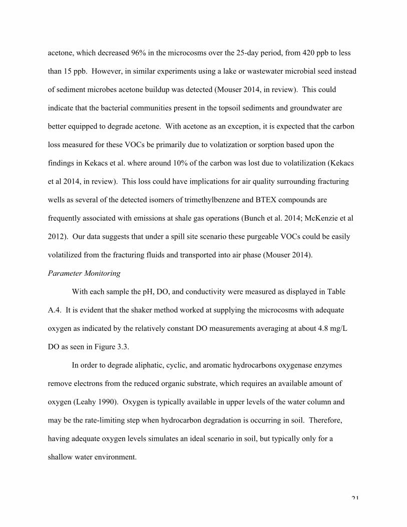
Figure 5.1. Temporal trends in A) density and B) viscosity of produced waters collected over a 328-day period from three Marcellus shale wells. Reported data were measured at a representative formation temperature of 60 °C. A two term, time-weighted power model and its fit (R2) are shown. Viscosity measurements of produced waters exhibited a similar rapid increase during the first

two weeks following hydraulic fracturing, with values nearing a plateau in the months after

Well 1Well 2Well 3

1.12

1.1

1.08

1.06

1.04

1.02

1.0

0.980 20 40 60 120 180 240 300 360

Dens

ity (g

/mL)

1.06

1.04

1.02

1.0

0.980 5 10 15

Days Post Fracturing

Dens

ity (g

/mL)

Inset

y=0.159x-0.4133+1.1R2=0.835

Visc

osity

, μ, (

mPa. s)

Days Post Fracturing0 20 40 60 120 180 240 300 360

Inset

y=0.392x-0.3272+1.15R2=0.509

A

BWell 1Well 2Well 3

Visc

osity

(mPa. s)

1.2

1.1

1.0

0.9

0.8

0.70 5 10 15

Days Post Fracturing

1.3

1.2

1.1

1.0

0.9

0.8

0.7

0.6

33

production began (Fig. 1B). Over the 11-month period, mean sample viscosity increased 26.5%

from 0.86 ± 0.04 mPa·s in injected fluid to 1.09 ± 0.004 mPa·s in the latest produced waters

when measured at 60 °C. Almost half (49%) of total viscosity change occurred within the first 9

days (Fig. 1B inset), and more than three-quarters (78%) within 49 days (Table S1). Sample

variability was higher for viscosity measurements, which affected the strength of a two term,

time-weighted power model (R2=0.509) used to describe the trend of increasing viscosity

through time (Fig. 5.1B).

While density and viscosity of produced waters generally increased with respect to time

after hydraulic fracturing, fluid physical properties also varied as a function of temperature.

Mean density of injected fluid (day 0) decreased by 2.0 ± 0.1% between 20 and 60 °C, while

mean density of produced water from day 328 decreased by 2.7 ± 1.7% across this same

temperature range (Fig. 5.2A).

34

Figure 5.2. Relationships between A) density and B) viscosity measured across a 20 to 60 ºC range for produced waters collected over a 328 day period from three Marcellus shale wells.

This suggests that temporal changes in solute concentration have little effect on the temperature-

dependent density of these fluids. In contrast, mean viscosity of injected fluids decreased 44.4 ±

8.6% from 20 to 60 °C, while brine fluids collected at day 328 decreased by only 34.2 ± 2.3%

(Fig. 5.2B), indicating viscosities of low-salinity injected fluids may be more sensitive to

changes in temperature than later produced brines. These observations are supported by data for

other saline waters, where greater salinity increases sensitivity of fluid density to changes in

temperature, while conversely decreasing the temperature sensitivity of viscosity (Sharqawy et

al. 2010). Analyses of Milli-Q water density at 20 °C were less than 0.8% different than reported

values, while samples evaluated at 60 °C deviated by 1.6%. Considering that these three wells

were drilled in one location of the greater Marcellus region, and recognizing that operators may

20 40 600

0.5

1.0

1.5

2.0

2.5

Temperature (o C)20 30 40 50 60

0.9

0.95

1.0

1.05

1.1

1.15

Temperature (o C)

Den

sity

(g/m

L)

A B

Day 328

Day 0Day 0

Day 328

Well 1Well 2Well 3

Vis

cosi

ty, μ

, (m

Pa. s

)Well 1Well 2Well 3

35

use variable ratios of fresh and recycled water in injected fluid formulations, these data should

not be considered representative of all Marcellus shale produced waters, but rather can be used to

constrain a realistic range of density and viscosity values for input to model evaluations (Table

A.5).

Examining the behavior of water molecules can help to explain these changes. Density is

decreased by an increase in temperature, for while mass is independent of temperature and

remains constant, the volume occupied by each water molecule increases with greater kinetic

(thermal) energy. Viscosity is the result of intermolecular forces between water molecules that

generate a certain magnitude of cohesion. As temperature increases, a greater kinetic energy

enables each molecule to more easily overcome the attractive intermolecular forces acting

between it and other nearby molecules, permitting the bulk fluid to flow more readily (Jones and

Talley 1933). The effect of salinity on density and viscosity is also understood at this scale. Fluid

density will increase if an added solute increases solution mass more than solution volume. In the

case of viscosity, the addition of

certain solutes leads to a preferential

arrangement of ions among water

molecules, such that perturbation of

the arrangement (i.e., fluid flow)

requires more energy (Jones and

Talley 1933).

In this context we looked to sample

fluid chemistry to explain changes in

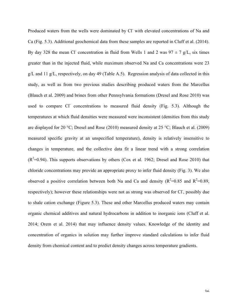
intrinsic physical properties. Figure 5.3. Relationships between density and dissolved inorganic components reported in this study and others (Blauch et al. 2009; Dresel and Rose 2010) for Pennsylvania brines and produced waters. A linear regression and its fit (R2) were used to describe the correlation between density and chloride (Cl-) concentrations using all data.

36

Produced waters from the wells were dominated by Cl- with elevated concentrations of Na and

Ca (Fig. 5.3). Additional geochemical data from these samples are reported in Cluff et al. (2014).

By day 328 the mean Cl- concentration in fluid from Wells 1 and 2 was 97 ± 7 g/L, six times

greater than in the injected fluid, while maximum observed Na and Ca concentrations were 23

g/L and 11 g/L, respectively, on day 49 (Table A.5). Regression analysis of data collected in this

study, as well as from two previous studies describing produced waters from the Marcellus

(Blauch et al. 2009) and brines from other Pennsylvania formations (Dresel and Rose 2010) was

used to compare Cl- concentrations to measured fluid density (Fig. 5.3). Although the

temperatures at which fluid densities were measured were inconsistent (densities from this study

are displayed for 20 °C; Dresel and Rose (2010) measured density at 25 °C; Blauch et al. (2009)

measured specific gravity at an unspecified temperature), density is relatively insensitive to

changes in temperature, and the collective data fit a linear trend with a strong correlation

(R2=0.94). This supports observations by others (Cox et al. 1962; Dresel and Rose 2010) that

chloride concentrations may provide an appropriate proxy to infer fluid density (Fig. 3). We also

observed a positive correlation between both Na and Ca and density (R2=0.85 and R2=0.89,

respectively); however these relationships were not as strong was observed for Cl-, possibly due

to shale cation exchange (Figure 5.3). These and other Marcellus produced waters may contain

organic chemical additives and natural hydrocarbons in addition to inorganic ions (Cluff et al.

2014; Orem et al. 2014) that may influence density values. Knowledge of the identity and

concentration of organics in solution may further improve standard calculations to infer fluid

density from chemical content and to predict density changes across temperature gradients.

37

Conclusion

In formations such as the Pennsylvania Marcellus shale, which can be more than 2 km below

ground surface and where geothermal gradients may be as high as 25 °C/km (Eckstein et al.

1982), changes in temperature likely impact not only chemical phenomena such as sorption and

precipitation-dissolution equilibria but also hydrodynamic processes including displacement and

mixing. Altered by such processes, mean densities of produced waters measured here decreased

by up to 2.7% over a 40 ºC temperature range and increased 9.8% over 11 months after hydraulic

fracturing. Mean viscosities, however, decreased by up to 44.4% and increased by 26.5%,

respectively, for the same temperature and time factors. To relate these observations to transport

models, changes in formation temperature and fluid chemistry will likely affect fluid viscosity

substantially more than fluid density, with a relative effect of greater flow rates for injected fluid

at formation depth and reduced flow rates for aged brine near the cooler surface. Considering

these findings, the authors suggest that models evaluating the potential migration of hydraulic

fracturing fluid across such depths take into account the dependence of fluid physical properties

on the timing of fluid release with respect to its chemical evolution, and on the geothermal

gradient of the formations through which it migrates.

38

Chapter 5

Further Research

In trying to determine the fate of fracturing fluid in the subsurface in the event of surface

spill during a drilling process, I simulated experimental conditions for aerobic degradation.

However, this many not represent other redox conditions that occur in the environment. In order

to fully understand how fracturing fluid degrades during the hydraulic fracturing process, anoxic,

and anaerobic batch microcosm experiments with more compacted soil, and rock should be

performed. These parameters will be more fitting for fracturing fluid degradation in deeper

environments, with limited or no oxygen resources. Contamination into deep aquifer could be a

result of an improperly cased well, downward vertical migration from the shallower depths, or

migration from the fractures. In order to conduct these studies, a different set of nutrients, and

materials should be supplied to these microcosms. Furthermore, studies surrounding bacteria

genomes that conduct this degradation could help lead to a better understanding of what nutrients

are needed for these metabolisms to occur, as well as more specific pathways of degradation.

These studies will help us understand the fate of the fluids in deeper subsurface conditions and

could provide more valuable information for understanding the risk associated with the migration

and fate of these compounds. Additionally, studies surrounding air quality should also be

considered when doing an environmental contamination study. VOCs can be easily air stripped

at a fracturing site, which raises concern of transport via air and inhalation. In order to best study

possible pathways of risks, all types of media need to be considered including water, soil, and air

experiments and sampling.

39

Appendix

Table A.1. Compounds and amounts used in preparing synthetic fracturing fluid (Kekacs et al 2014).

Component Disclosed Ingredients Mass (g) or Volume (ml) added per L SFF

Carrier/base fluid Source water (collected from Atwood Lake in Senecaville, Ohio) 896 ml

Proppant Sand (100 mesh sand produced by Unimin) 99 g Acid HCl (15% by mass) 3.5 g Fe control Citric acid 0.014 g Corrosion inhibitor (Weatherford AI600)

Ethylene glycol, dimethyl formamide, decanol, isopropanol, octanol, 2-butoxyethanol, proprietary compounds 0.007 ml

Friction reducer (Weatherford WFR-61LA)

Petroleum distillate, hydrotreated light, sodium chloride, chloride) 0.12 ml

Surfactant (Weatherford Revert flow)

Alcohol ethoxylated, isoporopanol, citrusturpenes, aromatic hydrocarbon mixture, naphthalene 0.47 ml

Clay stabilizer (Weatherford CC-120) Proprietary non-hazardous salt 0.44 ml

Gelling agent (Weatherford WGA 15L) Petroleum distillate, hydrotreated light, proprietary polymer 0.52 ml

Biocide (NALCO EC6110A) Glutaraldehyde, quaternary ammonium compound, ethanol 0.05 ml

Cross linker Ethylene glycol 0.008 g

Boric acid 0.004 g Ethanolamine 0.002 ml

Breaker Ammonium persulfate 0.005 g

pH adjustor K2CO3 0.018 g KOH 0.007 g

40

Table A.2. Complete MASI VOC Analysis Results with Cas. No, Compound name, and maximum detection limit (MDL). Adapted from Keckacs et al 2014.

Cas No. Compound MDL (ug/l)

Cas No. Compound MDL (ug/l)

630-20-6 1,1,1,2-Tetrachloroethane 0.16 75-25-2 Bromoform 0.17 71-55-6 1,1,1-Trichloroethane 0.22 74-83-9 Bromomethane 0.33 79-34-5 1,1,2,2-Tetrachloroethane 0.23 75-15-0 Carbon Disulfide 0.077 79-00-5 1,1,2-Trichloroethane 0.26 56-23-5 Carbon Tetrachloride 0.21 75-34-3 1,1-Dichloroethane 0.17 108-90-7 Chlorobenzene 0.059 75-35-4 1,1-Dichloroethene 0.25 75-00-3 Chloroethane 1.3

563-58-6 1,1-Dichloropropene 0.14 67-66-3 Chloroform 0.13 87-61-6 1,2,3-Trichlorobenzene 0.13 74-87-3 Chloromethane 0.12 96-18-4 1,2,3-Trichloropropane 0.27 124-48-1 Dibromochloromethane 0.17

120-82-1 1,2,4-Trichlorobenzene 0.13 74-95-3 Dibromomethane 0.31 95-63-6 1,2,4-Trimethylbenzene 0.11 75-71-8 Dichlorodifluoromethane 0.12 96-12-8 1,2-Dibromo-3-chloropropane 1.6 100-41-4 Ethylbenzene 0.11

106-93-4 1,2-Dibromoethane 0.26 87-68-3 Hexchlorobutadiene 0.23 95-50-1 1,2-Dichlorobenzene 0.12 74-88-4 Iodomethane 0.37

107-06-2 1,2-Dichloroethane 0.21 98-82-8 Isopropylbenzene 0.025 78-87-5 1,2-Dichloropropane 0.11 106-42-3 M,P-Xylene 0.21

108-67-8 1,3,5-Trimethylbenzene 0.081 1634-04-4 MTBE 0.23 541-73-1 1,3-Dichlorobenzene 0.094 75-09-2 Methylene Chloride 0.29 142-28-9 1,3-Dichloropropane 0.14 91-20-3 Napthalene 0.054 106-46-7 1,4-Dichlorobenzene 0.19 135-98-8 Sec-Butylbenzene 0.075 594-20-7 2,2-Dichloropropane 0.16 100-42-5 Styrene 0.11 78-93-3 2-Butanone 0.99 127-18-4 Tetrachloroethene 0.18

110-75-8 2-Chloroethylvinyl Ether 0.21 108-88-3 Toluene 0.15 95-49-8 2-Chlorotoluene 0.076 79-01-6 Trichloroethene 0.21

591-78-6 2-Hexanone 0.19 75-69-4 Trichlorofluoromethane 0.22 106-43-4 4-Chlorotoluene 0.17 108-05-4 Vinyl Acetate 0.20 99-87-6 4-Isopropyltoluene 0.088 75-01-4 Vinyl Chloride 0.27

108-10-1 4-Methyl-2-pentanone 0.12 1330-20-7 Xylenes (total) 0.88 67-64-1 Acetone 0.29 156-59-2 Cis-1,2-Dichloroethene 0.20

107-02-8 Acrolein 5.1 10061-01-5 Cis-1,3-Dichloropropene 0.051 107-13-1 Acrylonitrile 2.0 104-51-8 n-Butylbenzene 0.074 71-43-2 Benzene 0.13 103-65-1 n-propylbenzene 0.049

108-86-1 Bromobenzene 0.13 95-47-6 o-Xylene 0.15 74-97-5 Bromochloromethane 0.91 98-06-6 Tert-butylbenzene 0.088 75-27-4 Bromodichloromethane 0.21 156-60-5 Trans-1,2-Dichloroethene 0.25

10061-02-6 Trans-1,3-dichloropropene 0.13

41

Table A.3. Significant VOC compounds found from MASI analysis. Significance is based on reported concentrations and known health concerns. Table shows the percent loss (or percent gain), log removal of the compound and K degradation constant (days-1). The biotic concentrations are reported for initial concentrations, day 7, and 25th day. Compound structures from wikipedia.org.

42

Table A.4. Raw Data from Experiment including pH, DO, conductivity and temperature. Sample ID is same structure each time: (A/B)X-(1/2/3)-(0/N/D), where A represents abiotic or B represents biotic, X represents the day from beginning of experiment, 1/2/3 represents which of the three triplicates it is, and 0/N/D represents ratio of fracturing fluid to groundwater, with 0 being only groundwater, D being the 1:5 dilution, and N being non-diluted.

43

Sample ID Dissolved Oxygen (mg/L)

Conductivity (uS/cm)

pH Fluid Temperature

(C) B0-­‐1-­‐0   4.5   387   7.338   19.2  B0-­‐2-­‐0   4.44   368   7.54   18.9  B0-­‐3-­‐0   4.41   702   7.37   18.6  B0-­‐1  D   4.74   770   6.85   19.1  B0-­‐2  D   4.29   772   7.11   19  B0-­‐3-­‐D   4.48   757   6.995   19  B0-­‐1-­‐N   4.05   1187   3.295   19  B0-­‐2-­‐N   4.41   1187   3.129   19  B0-­‐3-­‐N   3.8   1771   2.974   18.8  A0-­‐3-­‐0   4.11   522   6.99   18.3  A0-­‐1-­‐0   3.1   506   7.226   19.6  A0-­‐2-­‐0   3.12   525   7.282   20.8  A0-­‐1-­‐D   3.1   683   7.09   20.2  A0-­‐2-­‐D   3.46   725   7.044   20.2  A0-­‐3-­‐D   3.21   725   6.969   20.1  A0-­‐1-­‐N   3.18   738   6.114   19.5  A0-­‐2-­‐N   3.14   1070   6.111   19.7  A0-­‐3-­‐N   3.3   1623   6.261   19.9  

B2-­‐1-­‐0   4.8   700   8.362   19.7  B2-­‐2-­‐0   4.85   690   8.441   19.7  B2-­‐3-­‐0   4.77   713   8.33   19.8  B2-­‐1-­‐D   4.13   816   8.044   19.8  B2-­‐2-­‐D   4.48   814   7.906   19.7  B2-­‐3-­‐D   4.46   801   8.027   19.4  B2-­‐1-­‐N   4.88   1482   5.744   18.8  B2-­‐2-­‐N   4.06   1485   6.593   19.2  B2-­‐3-­‐N   3.98   1496   6.748   19.4  

 B5-­‐1-­‐0   4.63   693   8.621   20.9  B5-­‐2-­‐0   5.58   700   8.552   19.8  B5-­‐3-­‐0   5.33   703   8.65   19.6  B5-­‐1-­‐D   5.26   720   8.307   19.2  B5-­‐2-­‐D   5.03   770   8.353   19.5  

Sample ID   Dissolved Oxygen (mg/L)  

Conductivity (uS/cm)   pH  

Fluid Temperature

(C)  B5-­‐3-­‐D   4.67   796   8.339   19.3  B5-­‐1-­‐N   3.94   1406   7.494   19.1  

44

B5-­‐2-­‐N   4.19   1558   7.064   19.1  B5-­‐3-­‐N   4.19   1532   6.869   18.7  

 B7-­‐1-­‐0   4.33   737   8.309   23.4  B7-­‐2-­‐0   4.87   744   8.354   23.6  B7-­‐3-­‐0   4.62   736   8.38   23.4  B7-­‐1-­‐D   4.24   663   8.124   23.1  B7-­‐2-­‐D   4.32   714   8.13   23.4  B7-­‐3-­‐D   4.52   875   8.074   23.2  B7-­‐1-­‐N   3.06   985   7.61   22.9  B7-­‐2-­‐N   2.83   1477   7.605   23.2  B7-­‐3-­‐N   1.8   1284   7.486   23.5  

 B25-­‐1-­‐0   4.43   574   8.162   21.3  B25-­‐2-­‐0   4.3   518   8.368   21.2  B25-­‐3-­‐0   4.47   696   8.392   21.4  B25-­‐1-­‐D   4.94   819   8.224   21.2  B25-­‐2-­‐D   4.26   805   8.365   21.3  B25-­‐3-­‐D   4.31   801   8.265   21.2  B25-­‐1-­‐N   4.22   938   8.031   21  B25-­‐2-­‐N   3.77   1476   8.125   21.3  B25-­‐3-­‐N   3.82   1671   7.964   21.2  A25-­‐1-­‐0   4.59   566   8.185   21.3  A25-­‐2-­‐0   5.23   566   8.122   21.2  A25-­‐3-­‐0   4.83   565   8.068   21.3  A25-­‐1-­‐D   4.87   779   7.878   21.2  A25-­‐2-­‐D   4.08   801   8.002   21.5  A25-­‐3-­‐D   4.48   771   7.892   21.3  A25-­‐1-­‐N   3.45   600   7.443   21.1  A25-­‐2-­‐N   4.55   1361   7.743   21.3  A25-­‐3-­‐N   4.29   1714   7.569   21.3  

Table A.5. Density Averaged and standard deviation values for each flowback fluid sample collected.

45

Table A.5(cont’d). Viscosity Average and Standard deviation (SD) values along with geochemical values of chlorine, sodium and calcium for each flowback sample collected.

46

References

Administration,  U.  S.E.I.Annual  Energy  Outlook  2013,  Early  Release.  In  U.S.  Department  of  Energy:  2013.    American  Gas  Association  (AGA)  (2012).  Identifying  Key  Economic  Impacts  of  Recent  Increase  in  U.S  Natural  Gas  Production.  May  2012.    Website.  http://www.aga.org    

47

Coates,  John;  Woodward,  Joan;  Allen,  Jon;  (1997).  Anaerobic  Degradation  of  Polycyclic  Aromatic  Hydrocarbons  and  Alkanes  in  Petroleum  Contaminated  Marine  Harbor  Sediments.  Applied  and  Environmental  Microbiology.    

EPA  (1993).  Behavior  and  Determination  of  Volatile  Organic  Compounds  in  Soil.  1993.  

EPA  (2011).  Fracking  and  associated  media  composition  in  Colorado.  In  US  EPA  Technical  Workshop  for  the  Hydraulic  Fracturing  Study:  Fate  &  Transport,  Arlington,  Virginia,  2011.    EPA  (2012).  Study  of  the  Potential  Impacts  of  Hydraulic  Fracturing  on  Drinking  Water  Resources:  Progress  Report.    FracFocus,  Chemical  Disclosure  Registry.  2014.  

Hayes,  T.  Sampling  and  Analysis  of  Water  Streams  Associated  with  the  Development  of  Marcellus  Shale  Gas;  2009.    Gassiat,  C.;  Gleeson,  T.;  Lefebvre,  R.;  McKenzie,  J.  (2013),  Hydraulic  fracturing  in  faulted  sedimentary  basins:  Numerical  simulation  of  potential  contamination  of  shallow  aquifers  over  long  time  scales.  Water  Resources  Research  2013,  49,  (12),  8310-­‐8327.    Jiang,  Mohan;  Hendrickson,  Chris;  VanBriesen,  Jeanne  (2013).    Life  Cycle  Water  Consumption  and  Wastewater  Gneration  Impacts  of  a  Marcellus  Shale  Gas  Well.    Environmental  Science  and  Technology.    Kekacs  Dan,  McHugh  Maggie,  Mouser  Paula.  (2015).    Temporal  Changes  of  Density  and  Viscosity  in  Produced  Fracturing  Fluids.    Journal  of  Environmental  Engineering.      Kekacs  Dan,  Drollette  Brian,  Brooker  Michael,  Plata  Desiree,  Mouser  Paula  (2014).    Aerobic  Biodegradation  of  Organics  in  Hydraulic  Fracturing  Fluids.    Biodegradation.    In  review.    Kassotis,  C.  D.,  Tillitt,  D.  E.,  Davis,  J.  W.,  Hormann,  A.  M.,&  Nagel,  S.  C.  (January  01,  2014).  Estrogen  and  androgen  receptor  activities  of  hydraulic  fracturing  chemicals  and  surface  and  groundwater  in  a  drilling-­‐dense  region.  Endocrinology,  155,  3,  897-­‐907.    Lutz,  B.  D.;  Lewis,  A.  N.;  Doyle,  M.  W.  (2013),  Generation,  transport,  and  disposal  of  wastewater  associated  with  Marcellus  Shale  gas  development.  Water  Resources  Research  49,  (2),  647-­‐656.  

Moran.    Michael  J.  Hamilton,  Pixie  A.  Zogorski,  John  S  (2006).  Volatile  Organic  Compounds  in  the  Nations  Ground  Water  and  Drinking-­‐Water  Supply  Wells—A  Summary.    

Mouser  J.  Paula,  Liu  Shuai,  Cluff  A.  Maryam,  McHugh  K.  Maggie,  Lenhart  John,  D.  MacRae  J.  (2014).    Biodegradation  of  Hydraulic  Fracturing  Fluid  Organic  Additives  in  Sediment-­‐Groundwater  Microcosms.    In  Review.  

National  Research  Council  (NRC),  2006.  Surface  Temperature  Reconstructions  For  the  Last  2,000  Years.  National  Academy  Press,  Washington,  DC.  

48

Olmstead,  S.  M.;  Muehlenbachs,  L.  A.;  Shih,  J.-­‐‑S.;  Chu,  Z.;  Krupnick,  A.  J.,  Shale  gas  development  impacts  on  surface  water  quality  in  Pennsylvania.  Proceedings  of  the  National  Academy  of  Sciences  2013,  110,  (13),  4962-­‐‑4967.  

Rozell,  Daniel;Reaven,  Sheldon  (2012).    Water  Pollution  Risk  Associated  with  Natural  Gas  Extraction  from  Marcellus  Shale.    Risk  Analysis  Vol  32  No.  8.    

Shaffer,  D.  L.;  Arias  Chavez,  L.  H.;  Ben-­‐Sasson,  M.;  Romero-­‐Vargas  Castrillón,  S.;  Yip,  N.  Y.;    Elimelech,  M.  (2013),  Desalination  and  Reuse  of  High-­‐Salinity  Shale  Gas  Produced  Water:  Drivers,  Technologies,  and  Future  Directions.  Environmental  Science  &  Technology  47,  (17),  9569-­‐9583.    Stringfellow,  W.T.,  J.K.  Domen,  M.K.  Camarillo,  W.L.  Sandelin,  and  S.  Borglin(2014).  Physical,  chemical,  and  biological  characteristics  of  compounds  used  in  hydraulic  fracturing.  Journal  of  Hazardous  Materials,  275:  37-­‐54.    US  Environmental  Protection  Agency  Office  of  Research  and  Development  (2012).  Progress  Report  Study  of  the  Potential  Impacts  of  Hydraulic  Fracturing  on  Drinking  Water  Resources.  

USGS  (2005).  Factors  Associated  with  Sources,  Transport,  and  Fate  of  Volatile  Organic  Compounds  in  Aquifers  of  the  United  States  and  Implications  for  Ground-­‐‑Water  Management  and  Assessments.    

Warner,  N.  R.;  Jackson,  R.  B.;  Darrah,  T.  H.;  Osborn,  S.  G.;  Down,  A.;  Zhao,  K.;  White,  A.;  Vengosh,  A.  (2012).  Geochemical  evidence  for  possible  natural  migration  of  Marcellus  Formation  brine  to  shallow  aquifers  in  Pennsylvania.  Proceedings  of  the  National  Academy  of  Sciences  2012,  109,  (30),  11961-­‐11966.    Yi,  T.;  Peden,  J.  M.  A  Comprehensive  Model  of  Fluid  Loss  in  Hydraulic  Fracturing.  Myers,  T.  (2012).  Potential  Contaminant  Pathways  from  Hydraulically  Fractured  Shale  to  Aquifers.  Ground  Water  2012,  50,  (6),  872-­‐882.