The path-independent M integral implies thecreep closure of englacial and subglacial

channels

Colin R. Meyer∗Graduate Research Assistant

John A. PaulsonSchool of Engineering and

Applied Sciences Harvard University,Cambridge, MA 02138,

Email: colinrmeyer@gmail.com

John W. HutchinsonProfessor, Fellow of ASME,

John A. PaulsonSchool of Engineering and

Applied Sciences, Harvard University,Cambridge, MA 02138,

Email: hutchinson@husm.harvard.edu

James R. RiceProfessor, Fellow of ASME,

John A. Paulson School of Engineering and Applied Sciences,and Department of Earth and Planetary Sciences,

Harvard University, Cambridge, MA 02138, Email: rice@seas.harvard.edu

Drainage channels are essential components of englacialand subglacial hydrologic systems. Here we use the M in-tegral, a path-independent integral of the equations of con-tinuum mechanics for a class of media, to unify descriptionsof creep closure under a variety of stress states surroundingdrainage channels. The advantage of this approach is thatthe M integral around the hydrologic channels is identical tosame integral evaluated in the far-field. In this way, the creepclosure on the channel wall can be determined as a functionof the far-field loading, e.g. involving antiplane shear as wellas overburden pressure. We start by analyzing the axisym-metric case and show that the Nye solution for the creep clo-sure of the channels is implied by the path-independence ofthe M integral. We then examine the effects of superimposingantiplane shear. We show that the creep closure of the chan-nels acts as a perturbation in the far-field, which we exploreanalytically and numerically. In this way, the creep closureof channels can be succinctly written in terms of the path-independent M integral and understanding the variation withapplied shear is useful for glacial hydrology models.

NomenclatureA Ice softnessεi j Strain fieldIi Strain rate tensor invariantsM Path-independent integralWs Strain energy densityW Flow potential

∗Corresponding author

ui Displacement field` Dimension, i.e. 2 or 3.m Homogeneity degree, Ws = σi jεi j/mn Rheological exponent, i.e. 3 for Glen’s lawp Isotropic ice pressurevi Velocity fieldxi Position fieldDi j Strain rate fieldσi j Stress fieldσ′i j Deviatoric stress field, σi j + pδi j

DE Effective strain rate,√

Di jDi j/2

τE Effective stress,√

σ′i jσ′i j/2

Ik Invariant of strain rate tensora Channel radius∆p Effective pressureσ0 Ice overburden pressure, ρigHρi Ice densityg Acceleration due to gravityH Ice thicknessp f Fluid pressure within channelγ f ar Far-field antiplane strain rateS Strain rate ratio, γ f ar/(A∆pn)

1 IntroductionGlacial melt water from surface ablation, precipitation,

and internal deformation drains via englacial conduits to thebase of the glacier where it is evacuated through a subglacialhydrologic network of channels melted into the ice or cav-ities in the sediments [1, 2, 3]. In this paper, we focus

To be published in J. Appl. Mech.-2017

on channelized drainage through Rothlisberger channels [2],where these channels are melted into the ice by the heat dis-sipation of the turbulently flowing melt water and close byviscous creep of the surrounding ice. We model these chan-nels as very long straight conduits that are oriented alongthe direction of glacier flow and we use a conserved integralapproach to derive the classical solution found by Nye [4]for the radial, or in-plane, creep closure velocity of the iceinto the channel. We then show how the creep closure ofthe channels increases when we take the downstream shearpresent within the ice column, referred to as antiplane shear,into account, such as in an ice stream shear margin.

Path-independent (conserved) integrals are importantmathematical tools that are often employed in mechanics asa method of solution to the equations or as a supplemen-tal constraint. Gunther [5], and independently Knowles andSternberg [6], introduced a path-independent integral for lin-ear elastic solid mechanics, which Budiansky and Rice [7]called the M integral. Using the Noether [8] procedure, the`-dimensional, linear elastic M integral is the conservationintegral that results from a self-similar scale change by theinfinitesimal factor γ, i.e.

x′α = xα + γxα and u′α(x′) = uα(x)+

(1− `

2

)γuα(x),

That is, coordinates xα and displacements uα are self-similarly scaled from the reference configuration [9]. In theframework of linearized kinematics, the strain is equal to thesymmetric part of the displacement ui gradient tensor as εi j =sym(∂ui/∂x j). We can then write a strain energy density Wsas a product of stresses σi j and strains εi j by Ws = σi jεi j/2.The general conserved integral resulting from the Noetherprocedure, with yα = x′α− xα and fα(x) = u′α(x

′)−uα(x), isgiven by

∮Γ

Wsyαnα +σαknk

[fα(x)− yβ

∂uα

∂xβ

]ds.

where this integral is a line integral for 2-dimensional prob-lems and a surface integral for 3-dimensional problems. Inthis way, the the M integral for a linear elastic material in twodimensions with linearized kinematics is given as

M =∮

Γ

Wsxαnα−σαknkxβ

∂uα

∂xβ

ds.

as written by [6].Budiansky and Rice [7] extended the earlier definitions

of M to a generalized elastic material with a strain energydensity Ws that is homogeneous of degree m in the strainsεi j, and, therefore, Ws = σi jεi j/m. Unfortunately, the [7]expression for the generalized M integral contains an error.Whether it is typographical, conceptual, or due to the print-ing process is unknown. He and Hutchinson [10] give a cor-rect expression (although without derivation) for the three-dimensional generalized M integral in a different geometry

than used here or in [7]: a closed 3-D void or flat crackof axially symmetric shape, such that stresses vary with zand

√x2 + y2. Rice [9] gives the correct Noether invariant

transformation to generate the `-dimensional M integral fora power law solid, although, subsequently, only writes theexpression of the M integral for the linear (m = 2) materialin two dimensions. To set the record straight, the generalizedM integral in two dimensions with combined in-plane andantiplane straining in the y-z plane, and with void aligned inthe x direction, is

M =∮

Γ

Wsxknk +σiknk

[(m−2

m

)ui− x j

∂ui

∂x j

]ds, (1)

where ni is the unit outer normal to the closed contour Γ

and s is arc length anti-clockwise around the path, suchthat n1ds = dx2 and n2ds = −dx1, where the tensor sub-scripts correspond as (x,y,z) = (x1,x2,x3) and (u,v,w) =(u1,u2,u3). Figure 1 shows the domain, the coordinate sys-tem, and a path of integration about a void.

The generalized definition of M for a power-law nonlin-ear elastic solid is exactly equivalent to the definition for apower-law nonlinear viscous fluid, where the displacementui is replaced by the velocity vi, and the strain εi j by thestrain rate Di j [11]. The strain rate is the symmetric part ofthe velocity gradient tensor, as Di j = sym(∂vi/∂x j). Underthe definition for a power-law viscous fluid, the elastic strainenergy density Ws is a replaced by a function called the flowpotential W . Just as dWs = σi jdDi j is an exact differential ingeneralised elasticity, dW is also an exact differential, satis-fying dW = σiidDi j. From here on, we will use the notationrelated to the flow of a viscous fluid. This change of notationand extension to viscous fluids allow us to apply the M inte-gral to the flow of ice in glaciers. In the notation of viscousfluids, the 2-dimensional M integral is written as

M =∮

Γ

Wxknk +σiknk

[(m−2

m

)vi− x j

∂vi

∂x j

]ds. (2)

We include a proof of the path independence of Equation (2)in appendix A.

The flow potential W for a viscous fluid is given as

∂W∂Di j

= σi j + pδi j, W =1m

σi jDi j, and dW = σi jdDi j,

where p (= −σkk/3) is the isotropic pressure (understoodhere as a Lagrange multiplier to enforce mass conservation,εkk = 0) and dW is an exact differential. The strain rates aredefined in terms of derivatives of the velocity vi as

Di j =12

(∂vi

∂x j+

∂v j

∂xi

)with

∂vk

∂xk= 0,

where the first condition shows that Di j is symmetric and bythe second condition (mass conservation for an incompress-ible substance) Di j is trace free.

Γ

~n

y

z

Fig. 1. Schematic of the path-independent M integral around avoid. The path of integration is Γ and the vector normal to this in-tegration path is ~n. The down glacier component is x which pointsout of the page, i.e. antiplane, the in-plane coordinates are y (acrossglacier) and z (depth).

1.1 Ice RheologyHere we describe how the rheology sets the value for the

parameter m. In glaciology, a commonly assumed rheologyis Glen’s law,

DE = AτnE , (3)

where DE is a function of the second invariant of the strainrate tensor, i.e. DE =

√Di jDi j/2, τE is defined in the same

way for the deviatoric stress tensor σ′i j = σi j + pδi j, and thesubscript E stands for effective. The two parameters are A,the ice softness, and n, the rheological exponent. The stan-dard value used in glaciology is n = 3 and is called Glen’slaw, which is appropriate for the typical values of stress andstrain rate encountered in the field [12]. Now relating devia-toric stress and strain rate tensors using Equation (3) impliesthat

Di j = Aτn−1E (σi j + pδi j) . (4)

Using this rheology the flow potential W can be determinedas

W =∫

σi jdDi j =n

n+1σi jDi j =

1m

σi jDi j,

and, thus, m = 1+ 1/n. From here on we will use the rhe-ological exponent n instead of m; for a Newtonian viscousfluid (or in linear elasticity), n = 1 and, therefore, m = 2, sothe term proportional to vi in Equation (2) will disappear.

In appendix B we show the general class of incompress-ible viscous fluids for which a flow potential W exists, whichis required for the M integral. All purely viscous incompress-ible fluids fall into the general class of Reiner-Rivlin fluids,which have a rheology given by

σi j =−pδi j +φ1(I2, I3)Di j +φ2(I2, I3)DinDn j,

where Ik is the kth invariant of the tensor Di j [13]. For athree-dimensional flow, the three invariants are

I1 = Dkk, I2 =12

DlmDml , I3 =13

DlmDmnDnl .

For a fluid that is incompressible,

I1 = 0.

Truesdell and Noll [14] assert that there is little exper-imental evidence for fluids with φ2 6= 0. This assertion isbased on Markovitz and Williamson [15], who find the poly-meric data collected by [16] to be incompatible with φ2 6= 0.In glaciology, it is not fully resolved whether Glen’s lawshould be expanded to include a dependence on I3 or φ2 6= 0.Glen [17] describes ice as a Reiner-Rivlin fluid and con-cludes that the experimental data show sufficient scatter towarrant further study. Baker [18] reviews the subsequent ex-periments in determining the effects of the third invariant onthe flow of ice and compares the results with his own ex-perimental set-up, which show that there is a significant de-pendence on I3. Still there appears to be little evidence thatφ2 6= 0 in ice. Such a fluid, as [17] notes, would to susceptibleto swelling or contraction in the direction perpendicular tothe plane of shear. Schoof and Clarke [19] exploit this gen-eration of deviatoric normal stress and use a Reiner-Rivlinfluid to model subglacial flutes by way of a secondary trans-verse flow. Here we show that only Reiner-Rivlin fluids thatare independent of I3 with φ2 = 0 have a flow potential W ,unless

∂φ1

∂I3=

∂φ2

∂I2.

Therefore, our analysis primarily applies for ice modeled us-ing a power-law rheology for ice, such as Glen’s law.

2 AnalysisTo analyze the creep closure of an drainage channel, it

is convenient to write M in polar coordinates and adopt a

circular path of radius r (ds = rdθ) as

M =∫ 2π

0

Wr−

(n−1n+1

)[σrrvr +σrθvθ +σrxvx]

−[

σrr∂vr

∂r+σrθ

∂vθ

∂r+σrx

∂vx

∂r

]r

rdθ. (5)

In this expression there are two types of terms: in-plane andantiplane. The in-plane terms are those in the r and θ direc-tion, such as vr, vθ, and σrθ. The antiplane terms, quantitieswith a subscript x, represent motion into and out of page as afunction of only the in-plane coordinates (using the standardglaciology coordinate system with z vertical, y across glacier,and x down glacier). We consider a very long channel withconstant ice thickness and, in this way, we can reduce a threedimensional problem to two dimensions where the quantitiesare homogeneous along x.

2.1 Nye solutionNye [4] derived the rate of closure of a circular channel

in a Glen rheology subject to a stress σrr(r = a) =−pw (wa-ter pressure) applied at the channel and the stress σrr(r →∞) = −σ0 = −ρigH (overburden ice pressure for a glacierof height H and density ρi) far away. By adding a uniformtensile stress σ0 to the mass of ice, we transform our prob-lem and apply a tensile stress σrr(r = a) = σ0− pw = ∆p atthe channel wall and a traction free condition at infinity. Weare able to do this without changing the problem because ofincompressibility and the pressure independence of Glen’slaw. Thus, the boundary conditions are

σrr(r = a) = σ0− pw = ∆p and σrr(r→ ∞) = 0.

The set-up for the problem and these conditions can be seenin Figure 2. What is also evident is that the problem is purelyin-plane and, therefore, we disregard the antiplane terms inEquation (5). Furthermore, the problem is axisymmetric andso we can neglect the in-plane shear terms. Hence, we havethe integral

M =∫ 2π

0

Wr2−

(n−1n+1

)σrrvrr−σrr

dvr

drr2

dθ. (6)

Mass conservation gives that

dvr

dr+

vr

r= 0,

and, therefore, we can simplify terms in Equation (6) as

M =∫ 2π

0

Wr2 +

2σrrvr

n+1r

dθ. (7)

r = a r→ ∞

σrr|r=a = ∆p

σrr|r→∞= 0

~Ur

Fig. 2. Nye problem set-up and boundary conditions. Blue arrowsindicate the creep closure of the ice (~Ur) and the turbulence in thechannel is suggested by the warm colors. (turbulent pipe flow simu-lation by [20]. photo credit: Noel Fitzpatrick)

For in-plane, axisymmetric motion, the flow potential W canbe written as

W =2n

n+1A−

1n D1+1/n

E =2n

n+1A−

1n

∣∣∣∣dvr

dr

∣∣∣∣1+1/n

.

This can be inserted into Equation (7). Then, using the factthat M is path independent, we can evaluate two contours:first, along r = a and, second, around r → ∞. These twocontours are chosen because these are the locations where theboundary conditions are applied. Starting with the latter, wecan see from mass conservation that dvr/dr→ 0 as r→ ∞.This means that the flow potential W also decays to zero inthe far-field. Although vrr is a constant as r→ ∞, the stressσrr(r→ ∞) = 0 (boundary condition) and, therefore, M = 0as r→ ∞.

Thus, the M integral around the channel must also bezero. Using the boundary condition σrr(r = a) = ∆p, massconservation, and the expression for the flow potential, wecan write Equation (7) as

M =2a

n+1

∫ 2π

0

nA−

1n |−vr|1+1/n a−1/n +∆pvr

dθ = 0.

Now, due to axisymmetry, the integrand must be independentof θ and is therefore equal to zero. Taking care with theabsolute value term, we can rearrange the integrand to find

vr(a) =−Aa(

∆pn

)n

, (8)

which is the Nye solution for the creep closure rate at theedge of the channel [4, 21].

This analysis can be easily extended to the case wherethe outer boundary is finite, i.e. where r = b on the outeredge in Figure 2. Following the same method, and usingDθθ = vr/r from geometry and Dθθ =−Drr from mass con-servation, we have that

M =2na2

n+1

∫ 2π

0

A−

1n

∣∣∣∣−vr(a)a

∣∣∣∣1+ 1n

+∆pvr(a)

na

dθ,

=2nb2

n+1

∫ 2π

0A−

1n

∣∣∣∣−vr(b)b

∣∣∣∣1+ 1n

dθ. (9)

Now the M integral around the outer edge of the domain isno longer zero. Since there is a constant volume flux throughany radius, i.e. 2πrvr = constant, we can related the radialvelocity at vr(r = a) to vr(r = a) as

avr(a) = bvr(b).

Solving for the creep closure rate at the edge of the channelvr(r = a) using Equation (9), we find that the finite domainNye solution is given as

vr(a) =−Aa

[1− (a/b)2/n]n

(∆pn

)n

,

which corroborates [22] and, also, reduces to the standardresult as b→ ∞.

2.2 Antiplane shearA natural extension for the M integral around an

englacial or subglacial channel is to include antiplane terms.These are the terms in Equation (5) that include x depen-dence. In glaciology, the antiplane terms can represent theshear flow of ice downstream, which is often ignored in thecreep closure of channels [23, 24, 25]. However, the down-stream flow decreases the effective viscosity of the ice, dueto the fact that Glen’s law is a shear-thinning rheology, andchannels close more quickly than in environments free of an-tiplane stress. Nye [4] and Glen [26] compare the Nye so-lution to tunnel closure measurements in the field and findthat some tunnels close much faster than predicted. Thus,the coupling between the in-plane creep closure and the an-tiplane motion of the glacier may be important in modelingsubglacial hydrologic systems.

Ice stream shear margins are also examples of where an-tiplane effects can affect the size of drainage channels. Perolet al. [27] give theoretical arguments for the existence of sub-glacial channels beneath ice stream shear margins which isbacked up by observations of running water at the base of thedormant Kamb ice stream [28]. Figure 3 shows a schematicfor an idealized ice stream shear margin, where the veloc-ity transitions from the fast flowing centerline to the nearlystagnant ridge. In the margin we have schematically drawn aRothlisberger [2] subglacial channel. Meyer et al. [29] show

α

R Channel Ice StreamRidge

x

yz

Fig. 3. Schemcatic for an idealized ice stream shear margin with aRothlisberger [2] subglacial channel. Surface ice velocity increasesaway from the margin and is nearly stagnant in the ridge (adaptedfrom [29]).

that the shear in the margin leads to faster closure velocitiesof drainage channels than would be predicted by the Nye so-lution, due to a decrease in effective viscosity from addingthe antiplane shear.

The problem set-up for including antiplane shear fol-lows Figure 2 with the additional boundary conditions

σrx|r=a = 0 and vx|r→∞= γ f arr cos(θ), (10)

which define the antiplane field. Using these boundary con-ditions, we evaluate the M integral around two contours: thechannel wall r = a as well as in the far-field r→ ∞.

2.2.1 Evaluation of the M integral at the channelWe start by evaluating M at the channel. We cancel the

in-plane shear terms (e.g. σrθ) and antiplane terms in Equa-tion (5), due to the boundary conditions in Equation (10).Thus, we arrive at

M =∫ 2π

0

Wr2−

(n−1n+1

)σrrvrr−σrr

∂vr

∂rr2

dθ.

Using mass conservation, we can write the radial velocityderivative as

∂vr

∂r=−vr

r− 1

r∂vθ

∂θ.

The second term in this expression can be neglected becauseit will always be zero when integrated around a closed loopfor a constant boundary stress. If we insert the effective pres-sure ∆p for the radial stress, we find that

M =∫ 2π

0

Wa2 +

2∆pn+1

vra

dθ, (11)

which is nearly identical to Equation (7) in symbols. The dif-ference is in the value of W . Along r = a with superimposedantiplane shear, we have that

Wr=a =2n

n+1A−1/nD1+1/n

E

∣∣∣∣r=a

,

=2n

n+1A−

1n

√(∂vr

∂r

)2

+

(12a

∂vx

∂θ

)21+1/n

,

where the shear term ∂vx/∂r was neglected due to the bound-ary condition specified in Equation (10). Inserting this ex-pression for Wr=a into Equation (11), we find that

M =2a2∆pn+1

∫ 2π

0

nA−

1n

∆p

[(∂vr

∂r

)2

+

(12a

∂vx

∂θ

)2] n+1

2n

+vr

a

dθ. (12)

2.2.2 Evaluation of M in the far-fieldFollowing the derivation of the Nye solution, we seek to

determine the value of M by evaluating the contour as r→∞.Starting from Equation (5), we now cancel all the in-planeterms, as they must decay as r→ ∞. This leaves us with

M =∫ 2π

0

Wr2−

(n−1n+1

)σrxvxr−σrx

∂vx

∂rr2

dθ.

We star by assuming that the antiplane fields are given by theboundary conditions, we have that

vx = γ f arr cos(θ) and σrx = A−1/n(γ f ar/2)1/n cos(θ),

which is a state of constant strain rate. Inserting these ex-pressions into M gives

M =∫ 2π

0

W − 2n

n+1(2A)−1/n

γ1+1/nf ar cos2(θ)

r2 dθ.

Evaluating W as r→ ∞ gives

W |r→∞=

2nn+1

A−1/n (γ f ar/2)1+1/n .

Thus, the integral for M as r→ ∞ reduces to

M =n

n+1(2A)−1/n

γ1+1/nf ar

∫ 2π

0

1−2cos2(θ)

r2 dθ = 0,

using the half-angle formula for cos(θ). In order for M tobe finite, this integral must be zero because of the r2 term in

the integrand. However, this integral does not represent thefull far-field contributions to M. The boundary conditionsrepresent a constant strain rate, a situation where M = 0 andthis evaluation of M in the far-field disregards the couplingbetween the antiplane and in-plane motion. Therefore, wemust retain a small perturbation away from a constant back-ground strain rate.

2.2.3 Far-field perturbationIn the far-field, we consider a perturbation from the con-

stant antiplane strain rate boundary condition. We write thefar-field velocities in Cartesian coordinates as

vx = γ f ary+εh(y,z), vy = εg(y,z), and vz = ε f (y,z).

Here ε is an unknown small parameter and f (y,z), g(y,z),and h(y,z) are unknown functions. To first order in ε, theeffective strain rate is given as

DE =γ f ar

2

√1+

2ε

γ f ar

∂h∂y

+O(ε2).

Consequently, the antiplane problem in the far-field is cou-pled to the in-plane motions through ε and we are able toignore the velocities v and w. Thus, we concentrate on writ-ing an equation for h(y,z). The antiplane stresses are givenby

σyx = A−1/nD(1−n)/nE

(γ f ar

2+

ε

2∂h∂y

)σzx = A−1/nD(1−n)/n

Eε

2∂h∂z

.

Inserting the effective strain rate and linearizing the stressabout ε gives

σyx =

[A

2γ f ar

]1/n(1+

ε

nγ f ar

∂h∂y

),

σzx =

[A

2γ f ar

]1/nε

γ f ar

∂h∂z

.

We then insert the linearized stress into the force balanceequation

∂σxy

∂y+

∂σyz

∂z= 0,

and we find that

1n

∂2h∂y2 +

∂2h∂z2 = 0.

By making the transformation, η =√

ny, we can write thisequation as

∇2h = 0,

i.e. Laplace’s equation with ∇ = (∂η,∂z). If we return topolar coordinates, now with

r =√

η2 + z2 and θ = arctan(

zη

),

we can write

h = rλ f (θ).

Inserting this ansatz into Laplace’s equation for h, we findthat

f = Bcos(kθ) and λ =±k,

where k is some unknown integer. The term proportionalto sin(kθ) can be ignored due to symmetry and the positivesolutions for λ can be disregarded as they are singular as r→∞. The term that decays the slowest is k =−1 and, therefore,we have

h =Br

cos(θ) =Br

cos(

arctan(

tan(θ)√n

))√

1+(n−1)cos2(θ)

, (13)

which we refer to as

h(r,θ) =Br

χ(θ).

Now inserting the perturbation ansatz h = εrλχ(θ) into theM integral in the far-field, we find that

M = ε

[γ f ar

2A

]1/n

rλ+1∫ 2π

0

λcos(θ)χ− sin(θ)χ′

−2(n−1)

n+1

[λcos3(θ)χ− 1

2cos(θ)sin(2θ)χ′

]−n−1

n+1(λ+1)cos(θ)χ+2λcos(θ)χ dθ,

where we have incorporated the unknown factor B into ε asthe unknown far-field amplitude. We know that λ =−1 and,therefore, we have that

M = ε

[γ f ar

2A

]1/n ∫ 2π

0

2(n−1)n+1

[cos3(θ)χ

+sin(θ)cos2(θ)χ′]+2cos(θ)χ dθ,

which is of the form

M = ε

[γ f ar

2A

]1/n

IM(n),

where IM(n) is given by

∫ 2π

0

2(n−1)n+1

[cos3(θ)χ +sin(θ)cos2(θ)χ′

]+2cos(θ)χ dθ,

Inserting our expression for χ(θ) from Equation (13), wecan integrate over θ numerical to find IM(n). For n = 3, i.e.Glen’s law for ice, we find that

I(3) =−0.113 . . .

This integral should be negative because in vx = γ f ary +εh(y,z) the antiplane velocity should be less than the bound-ary value as it approaches the edge.

Now, to determine the far-field amplitude factor ε, weneed to know the behavior of vz for small r, which requiressolving the fully coupled (in-plane and antiplane) PDE. Si-multaneously, the path independence of the M integral relatesthe perturbation integral in the far-field to the integral aroundthe channel, i.e. Equation (12). This gives

M =2a2∆pn+1

∫ 2π

0

nA−

1n

∆p

[(∂vr

∂r

)2

+

(1

2a∂vx

∂θ

)2] n+1

2n

+vr

a

dθ.

= ε

[γ f ar

2A

]1/n

IM(n). (14)

Thus, the perturbation amplitude ε is related to the unknownstrain rates at the edge of the channel. Furthermore, we cansee that that if vx = 0 (or if vx is a function of r only), thenthis integral reduces to the integral for the Nye solution andε = 0.

2.2.4 Nondimensional equations and numericsWe now write the expression for M in far-field nondi-

mensionally. The natural lengthscale is the channel radiusand, therefore, we write r = aR, where R is the nondimen-sional radial coordinate (using capital letters to denote nondi-mensional variables). We proceed by using the boundaryconditions to scale the stress and velocity. For the in-planecomponents of stress, ∆p is a sensible scaling. This leads toa scaling for the in-plane velocity, by dimensional argumentsalone, that is reminiscent of the Nye solution (Equation (8)),i.e. vr = Aa∆pnVr. From the antiplane boundary conditionswe can see that vx = γ f araVx. It is evident immediately thatthe in-plane and antiplane velocities do not scale in the samemanner and, thus, a logical control parameter for the systemis their ratio S, which is

S =γ f ar

A∆pn ,

S10

-710

-510

-310

-110

110

310

5

M

10-8

10-6

10-4

10-2

100

102

104

106

108

Minner

Mouter

M ∼ S(n+1)/n

M ∼ S1/n

Fig. 4. Numerical evaluation of M at the edge of the channel Minnerand in the far-field Mouter at R=500. The scalings show that for S1, M ∼ S1/n and for S 1, M ∼ S(n+1)/n. Numerical artifactslead to negative values for Minner when S is small, therefore thesesimulations are omitted but yield absolute values close to Mouter .

and represents the importance of antiplane shearing to in-plane creep closure [29]. Using S we can rewrite the an-tiplane velocity as vx = Aa∆pnSVx.

Using these scalings we can rewrite M as

M = a2A∆pn+1M,

where we immediately drop the variable hat. Thus, Equation14 gives

M =2

n+1

∫ 2π

0

n

[(∂Vr

∂R

)2

+S2

4

(∂Vx

∂θ

)2] n+1

2n

+Vr

dθ,

=ε

a2A∆pn

(S2

)1/n

IM(n). (15)

When the far-field of the domain is dominated by anitplaneshear, we have that S 1 and the appropriate scaling for ε is

ε = κγ f ara2,

where κ is now a constant related to the unknown strain ratesat the edge of the channel. When S 1, we scale ε usingthe Nye strain rate as ε = κA∆pna2. From this definition ofε, we can see that M in the far-field is either

M =κIM(n)

21/n S1/n (S 1) orκIM(n)

21/n S(n+1)/n (S 1).

Although we cannot solve for the constant κ analyti-cally, we can its value by numerical simulations. We im-plement the numerical method described in Meyer et al. [29]

in the existing finite element software COMSOL [30]. Thesesimulations allows us to compute the value of M as a func-tion of the strainrate ratio S, which is shown in figure 4. Thetwo regimes, where M scales as M ∼ S1/n for S 1 andM ∼ S1/n for S 1 are clearly visible. The best-fit value ofκ determined from the simulations is given by

κ =−2.45 (S 1) or κ =−86.97 (S 1).

These results show that as amount of antiplane shear withrespect to in-plane shear is increased, as measured by an in-crease in the strain rate ratio S, the M integral also increases.This is due to a simultaneous increase in both the creep clo-sure velocity Vr as well as the antiplane straining along theedge of the channel. The increase in channel closure veloc-ity is due to a decrease in effective viscosity, as described inMeyer et al. [29].

We now describe the evolution of the creep closure ve-locity as a function of S. When there is very little antiplanemotion as compared to in-plane straining, the creep closurevelocity is given by the Nye solution, Equation (8), which iswritten nondimensionally as

Vr =−n−n

R.

When the deformation is dominated by antiplane motion, i.e.S 1, the effective strain rate scales as εE ∼ S. The radialforce balance gives that the averaged creep closure velocityaround the channel is given as

Vr ∼−S(n−1)/n, (16)

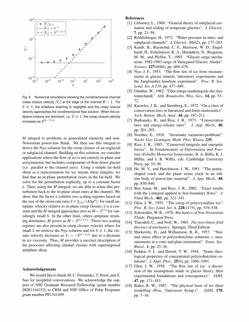
where more details are provided in [29]. In figure 5, we showthe two limits of the creep closure velocity: for S 1, thesimulations approach the Nye solution and for S 1, weverify the scaling given in Equation (16).

This increase in creep closure velocity due to the ad-dition of antiplane shear is consistent with the increase intunnel closure velocities observed by Nye [4] and Glen [26]due to changes in the glacier stress state. Furthermore, theincrease in creep closure velocity due to antiplane strainingis analogous to the Rice and Tracey [31] effect where thegrowth of voids is strongly enhanced by triaxiality. Intu-itively, the in-plane creep closure velocity for large S growsless than linearly with S as the antiplane field only influencesthe in-plane motion through the viscosity. The consequenceis that the dominant balance for large S in Equation (15) isstill between the perturbation in the far field and the antiplaneshear at the channel wall.

3 Concluding remarksIn this paper, we apply the path-independent M integral

to the creep of ice around subglacial and englacial channels.We correct a longstanding error in the implementation of the

S10

-710

-510

-310

-110

110

310

5

|Vr|

10-3

10-1

101

103

|Vr|R=1

|Vr| = n−n

|Vr| ∼ S(n−1)/n

Fig. 5. Numerical simulations showing the nondimensional channelcreep closure velocity |Vr| at the edge of the channel R = 1. ForS 1, the antiplane straining is negligible and the creep closurevelocity approaches the nondimensional Nye solution. When the an-tiplane motions are dominant, i.e. S 1, the creep closure velocityincreases as S(n−1)/n.

M integral to problems in generalized elasticity and non-Newtonian power-law fluids. We then use this integral toderive the Nye solution for the creep closure of an englacialor subglacial channel. Building on this solution, we considerapplications where the flow of ice is not entirely in-plane andaxisymmetric but includes components of flow down glacier(i.e. parallel to the channel axis). Using a simple far-fieldshear as a representation for ice stream shear margins, wefind that an in-plane perturbation exists in the far-field. Wesolve for the perturbation explicitly, up to a constant factorε. Then, using the M integral, we are able to relate this per-turbation back to the in-plane strain rates at the channel. Weshow that the factor ε exhibits two scaling regimes based onthe size of the strain rate ratio S≡ γ f ar/(A∆pn): for small an-tiplane velocity relative to in-plane creep closure, ε is a con-stant and the M integral approaches zero as M∼ S1/n for van-ishingly small S. In the other limit, where antiplane strain-ing dominates, M grows as M ∼ S(n+1)/n. These two scalingregimes are also present in creep closure velocity where forsmall S we retrieve the Nye solution and for S 1, the clo-sure velocity increases as Vr ∼ −S(n−1)/n due to a decreasein ice viscosity. Thus, M provides a succinct description ofthe processes affecting channel closure with superimposedantiplane shear.

AcknowledgementsWe would like to thank M. C. Fernandes, T. Perol, and Z.

Suo for insightful conversations. We acknowledge the sup-port of NSF Graduate Research Fellowship (grant numberDGE1144152) to CRM and NSF Office of Polar Programsgrant number PP1341499.

References[1] Lliboutry, L., 1968. “General theory of subglacial cav-

itation and sliding of temperate glaciers”. J. Glaciol.,7, pp. 21–58.

[2] Rothlisberger, H., 1972. “Water pressure in intra- andsubglacial channels”. J. Glaciol., 11(62), pp. 177–203.

[3] Kamb, B., Raymond, C. F., Harrison, W. D., Engel-hardt, H., Echelmeyer, K. A., Humphrey, N., Brugman,M. M., and Pfeffer, T., 1985. “Glacier surge mecha-nism: 1982-1983 surge of Variegated Glacier, Alaska”.Science, 227(4686), pp. 469–479.

[4] Nye, J. F., 1953. “The flow law of ice from measure-ments in glacier tunnels, laboratory experiments andthe Jungfraufirn borehole experiment”. Proc. R. Soc.Lond. Ser. A 219, pp. 477–489.

[5] Gunther, W., 1962. “Uber einige randintegrale der elas-tomechanik”. Abh. Braunschw. Wiss. Ges., 14, pp. 53–72.

[6] Knowles, J. K., and Sternberg, E., 1972. “On a class ofconservation laws in linearized and finite elastostatics”.Arch. Ration. Mech. Anal., 44, pp. 187–211.

[7] Budiansky, B., and Rice, J. R., 1973. “Conservationlaws and energy-release rates”. J. App. Mech., 40,pp. 201–203.

[8] Noether, E., 1918. “Invariante variations-probleme”.Nachr. Ges. Gottingen, Math. Phys. Klasse, 235.

[9] Rice, J. R., 1985. “Conserved integrals and energeticforces”. In Fundamentals of Deformation and Frac-ture (Eshelby Memorial Symposium), B. A. Bilby, K. J.Miller, and J. R. Willis, eds. Cambridge UniversityPress, pp. 33–56.

[10] He, M. Y., and Hutchinson, J. W., 1981. “The penny-shaped crack and the plane strain crack in an infi-nite body of power-law material”. J. App. Mech., 48,pp. 830–840.

[11] Ben Amar, M., and Rice, J. R., 2002. “Exact resultswith the j-integral applied to free-boundary flows”. J.Fluid Mech., 461, pp. 321–341.

[12] Glen, J. W., 1955. “The creep of polycrystalline ice”.Proc. R. Soc. Lond. Ser. A, 228(1175), pp. 519–538.

[13] Schowalter, W. R., 1978. Mechanics of Non-NewtonianFluids. Pergamon Press.

[14] Truesdell, C., and Noll, W., 1965. The non-linear fieldtheories of mechanics. Springer, Third Edition.

[15] Markovitz, H., and Williamson, R. B., 1957. “Nor-mal stress effect in polyisobutylene solutions. i. mea-surements in a cone and plate instrument”. Trans. Soc.Rheol., 1, pp. 25–36.

[16] Padden, F. J., and Dewitt, T. W., 1954. “Some rheo-logical properties of concentrated polyisobutylene so-lutions”. J. Appl. Phys., 25(9), pp. 1086–1091.

[17] Glen, J. W., 1958. “The flow law of ice: a discus-sion of the assumptions made in glacier theory, theirexperimental foundations and consequences”. IAHS,47, pp. 171–183.

[18] Baker, R. W., 1987. “The physical basis of ice sheetmodelling (Proc. Vancouver Symp.)”. IAHS, 170,pp. 7–16.

[19] Schoof, C., and Clarke, G. K. C., 2008. “A model forspiral flows in basal ice and the formation of subglacialflutes based on a Reiner-Rivlin rheology for glacialice”. J. Geophys. Res., 113(B5).

[20] Feldmann, D., and Wagner, C., 2012. “Direct numeri-cal simulation of fully developed turbulent and oscilla-tory pipe flows at Reτ = 1440”. J. Turbul., 13, pp. 1–28.

[21] Cuffey, K. M., and Paterson, W. S. B., 2010.The Physics of Glaciers (Fourth Edition). ISBN9780123694614. Elsevier.

[22] Evatt, G. W., 2015. “Rothlisberger channels with fi-nite ice depth and open channel flow”. Ann. Glaciol.,50(70), pp. 45–50.

[23] Schoof, C., 2010. “Ice-sheet acceleration driven bymelt supply variability”. Nature, 468(7325), pp. 803–806.

[24] Bartholomous, T. C., Anderson, R. S., and Anderson,S. P., 2011. “Growth and collapse of the distributedsubglacial hydrologic system of Kennicott Glacier,Alaska, USA, and its effects on basal motion”. J.Glaciol., 57(206), pp. 985–1002.

[25] Hewitt, I. J., 2013. “Seasonal changes in ice sheet mo-tion due to melt water lubrication”. Earth Planet. Sci.Lett., 371, pp. 16–25.

[26] Glen, J. W., 1956. “Measurement of the deformationof ice in a tunnel at the foot of an ice fall”. J. Glaciol.,2(20), pp. 735–745.

[27] Perol, T., Rice, J. R., Platt, J. D., and Suckale, J.,2015. “Subglacial hydrology and ice stream margin lo-cations”. J. Geophys. Res., 120(7), pp. 1352–1368.

[28] Vogel, S. W., Tulaczyk, S., Kamb, B., Engelhardt, H.,Carsey, F. D., Behar, A. E., Lane, A. L., and Joughin, I.,2005. “Subglacial conditions during and after stoppageof an Antarctic Ice Stream: Is reactivation imminent?”.Geophys. Res. Lett., 32.

[29] Meyer, C. R., Fernandes, M. C., Creyts, T. T., andRice, J. R., 2016. “Effects of ice deformation onRothlisberger channels and implications for transitionsin subglacial hydrology”. J. Glaciol., 62(234), pp. 750–762.

[30] COMSOL, 2006. COMSOL Multiphysics: Version 4.3.COMSOL.

[31] Rice, J. R., and Tracey, D. M., 1969. “On the ductileenlargement of voids in triaxial stress fields”. J. Mech.Phys. Solids, 17(3), pp. 201–217.

Appendix A: Proof of the path independence of M

Here we start with the two dimensional generalized Mintegral as written in Equation (2) with m = 1+1/n, i.e.

M =∮

Γ

Wxknk−σiknk

[(n−1n+1

)vi + x j

∂vi

∂x j

]ds,

where Γ is a closed path, as shown in Figure 1. We use thedivergence theorem to write this integral as

M =∮

Ω

∂

∂xk

(Wxk−σik

[(n−1n+1

)vi + x j

∂vi

∂x j

])dA.

The M integral is path independent if the terms inside thearea integral are zero. That is, if

∂

∂xk

(Wxk−σik

[(n−1n+1

)vi + x j

∂vi

∂x j

])= 0.

Taking the derivatives we find that

∂W∂xk

xk +W∂xk

∂xk− ∂σik

∂xk

[(n−1n+1

)vi + x j

∂vi

∂x j

]−σik

[(n−1n+1

)∂vi

∂xk+

∂x j

∂xk

∂vi

∂x j+ x j

∂2vi

∂x j∂xk

]= 0. (17)

The equilibrium equations are

∂σik

∂xk= 0,

which allow us to cancel the third group of terms in Equation(17) and, therefore, write

∂W∂xk

xk+W∂xk

∂xk−σik

[(n−1n+1

)∂vi

∂xk+

∂x j

∂xk

∂vi

∂x j+ x j

∂2vi

∂x j∂xk

]= 0.

The derivatives of coordinates lead to Kronecker delta func-tions as

∂xi

∂x j= δi j,

where in two dimensions, δkk = 2 and thus,

∂W∂xk

xk+2W−σik

[(n−1n+1

)∂vi

∂xk+δ jk

∂vi

∂x j+ x j

∂2vi

∂x j∂xk

]= 0.

We can simplify this expression slightly by multiplyingthrough by the stress and combining like terms as

∂W∂xk

xk +2W − 2nn+1

σik∂vi

∂xk−σikx j

∂2vi

∂x j∂xk= 0.

The strain rate energy density function W can be related tothe stress and strain rates as

W =n

n+1σi jDi j =

nn+1

σi j∂vi

∂x j.

This allows us to write

∂W∂xk

xk +2W −2W −σi j∂2vi

∂xk∂x jxk = 0.

Canceling the 2W terms, we can use the chain rule to relatespatial derivatives on W to derivatives of strain as

∂W∂Di j

∂Di j

∂xkxk−σi j

∂2vi

∂xk∂x jxk = 0.

If W is written to depend symmetrically on Di j, with con-straint Dkk = 0, then

σi j + pδi j =∂W∂Di j

,

and thus, the integrand is

σi j∂Di j

∂xkxk−σi j

∂2vi

∂xk∂x jxk = 0,

where the isotropic components of the stress tensor cancelwhen multiplied by ∂Di j/∂xk because ∂Dll/∂xk = 0. Now,using the symmetry of the stress tensor, we have that

σi j∂2vi

∂xk∂x jxk−σi j

∂2vi

∂xk∂x jxk = 0,

which is zero. Thus, we have shown that the M integral,written as

M =∮

Γ

Wxknk−σiknk

[(n−1n+1

)vi + x j

∂vi

∂x j

]ds,

is path independent.

Appendix B: Flow potential for a Reiner-Rivlin fluidA Reiner-Rivlin fluid is an incompressible fluid (I1 =

Dkk = 0) for which

σi j =−pδi j +φ1(I2, I3)Di j +φ2(I2, I3)DinDn j, (18)

where σi j is the stress tensor, Di j is the symmetric part of thevelocity gradient tensor, p is the isotropic pressure, and Ik isthe kth invariant of the tensor Di j [13]. By writing the stressas an isotropic matrix function of Di j, assuming a symmetricdependence on Di j and D ji, and expanding this function ofas a power series, we can use the Cayley-Hamilton theoremto show that the stress is a quadratic polynomial in Di j withcoefficients that are functions of the invariants of Di j. For an

incompressible fluid with isotropic pressure, this reduces toEquation (18).

Here we ask what is the most general fluid rheology thatstill posses a flow potential, i.e. where dW is a perfect differ-ential of σi jdDi j. This requires that

∂σi j

∂Dkl=

∂σkl

∂Di j, (19)

which is called Maxwell reciprocity. For an incompressiblefluid, we include pressure as a Lagrange multiplier to enforcemass conservation, and write that

∂

(σ′i j + pδi j

)∂Dkl

=∂(σ′kl + pδi j

)∂Di j

,

where the isotropic pressure p is independent of the strainrate. This shows that the deviatoric stress also satisfiesMaxwell reciprocity.

If we insert the Reiner-Rivlin fluid rheology into Equa-tion (19), we find that

(∂φ1

∂I3− ∂φ2

∂I2

)(Di jDknDnl−DklDinDn j) = 0.

Now since Di jDknDnl 6= DklDinDn j for all i, j, k, and l, theonly way for this condition to be satisfied for all flows is for

∂φ1

∂I3=

∂φ2

∂I2. (20)

This condition also arises from an equality requirementof the mixed partial derivatives of the flow potential W . If westart with the invariants of Di j, given as

I1 = Dkk, I2 =12

DlmDml , I3 =13

DlmDmnDnl ,

we can write the relationship between the flow potential andthe stress as

σi j + pδi j =∂W∂Di j

=∂W∂I2

∂I2

∂Di j+

∂W∂I3

∂I3

∂Di j. (21)

Now using the facts that

∂Di j

∂Dkl= δikδ jl ,

∂I2

∂Dkl= Dkl and

∂I3

∂Dkl= DknDnl ,

we have that

σi j + pδi j =∂W∂Di j

=∂W∂I2

Di j +∂W∂I3

DinDn j. (22)

from which we can see that Equation (22) is Reiner-Rivlinfluid with

φ1 =∂W∂I2

and φ2 =∂W∂I3

.

Thus, a requirement for W to exist, and to be a perfect dif-ferential of σi jdDi j as is required to write Equation (21), isthat

∂2W∂I2∂I3

=∂2W

∂I3∂I2,

which implies that

∂φ1

∂I3=

∂φ2

∂I2,

just as was found in Equation (20).A class of Reiner-Rivlin fluids that always satisfies the

condition in Equation (20) are those for which φ1 is a func-tion of I2 solely and φ2 = 0. This is the rheological structureof Glen’s law in glaciology and, therefore, a flow potentialW will always exist.