Page 1
University of ConnecticutOpenCommons@UConn
Master's Theses University of Connecticut Graduate School
5-11-2013
The Pilot Study of Students’ Perception onTeachers’ Moral Character Scale in IndonesiaIfa H. MisbachUniversity of Connecticut, [email protected]
This work is brought to you for free and open access by the University of Connecticut Graduate School at OpenCommons@UConn. It has beenaccepted for inclusion in Master's Theses by an authorized administrator of OpenCommons@UConn. For more information, please [email protected] .
Recommended CitationMisbach, Ifa H., "The Pilot Study of Students’ Perception on Teachers’ Moral Character Scale in Indonesia" (2013). Master's Theses.443.https://opencommons.uconn.edu/gs_theses/443
Page 2
The Pilot Study of Students’ Perception on Teachers’ Moral Character Scale in Indonesia
Ifa Hanifah Misbach
University of Connecticut, 2013
A Thesis
Submitted in Partial Fulfillment of the
Requirements for the Degree of
Master of Arts
At the
University of Connecticut
2013
Page 3
APPROVAL PAGE
Masters of Arts Thesis
The Pilot Study of Students’ Perception on Teachers’ Moral Character Scale in Indonesia
Presented by
Ifa Hanifah Misbach
Major Advisor________________________________________________________________
Scott Brown
Associate Advisor_____________________________________________________________
Megan Welsh
Associate Advisor_____________________________________________________________
Jim O’Neil
University of Connecticut
2013
Page 4
Abstract
The purpose of this study is to develop a new instrument of Students’ Perception on
Teacher’s Moral Character Scale (SPoTMCS). The sample consisted of 12th
grade Indonesian
students (n=228), completing the SPoTMCS using a-paper-and-pencil format. This report
describes the results of the inter-correlation of items, and Cronbach‟s Alpha to calculate and
estimate of the internal reliability. To support a questionnaire development of SPoTMCS, factor
analysis procedures were also undertaken to determine the number of factors necessary to
explain the interrelationship among a set of dimensions of moral character and the underlying
dimensions of the construct of moral character in SPoTMCS. Using principal component
analysis (PCA) and oblimin rotation, the scale yielded three factors: Justice, Mercy, and
Tenderness. Additionally, there were two new interesting findings from this pilot study. The
demographic information and the distribution of each item were presented to explain the
uniqueness of the cultural model education in Indonesia.
Page 5
Chapter 1
Statement of the Problem
Morally, students in Indonesia today face a crisis of needing good role models from their
teachers. Schools are no longer documented as the renewal places of the educational growth in
fostering students‟ moral character (D. Joesoef, Personal Communication, June 21, 2011). On the
other hand, the culture of education model in Indonesia possesses a belief system that teachers
have a privileged status as outstanding role models (Thomas, 1962). Although teachers may not
see themselves as role models, they are trusted to serve as role models to inspire and motivate
students to do their best. In fact, teachers, as the traditional role models, continue to disappoint
the Indonesian society by facilitating many bad and/or demoralized behaviors during the Ujian
Nasional (National Examination), shortened as UN (Andie, 2012). From 2005 to 2012, the
escalation in the number of teachers‟ misbehaviors has increased by more than 750 cases since
the first UN was implemented (Jibi, 2012).
Many education experts in Indonesia argue that the misleading implementation of UN
causes teachers to do many demoralized behaviors, such as manipulating students‟ grades,
distributing the answers, and even worse, intimidating students to share their answers with the
whole class. On the other hand, The United Federation of Indonesian Teachers reports that
teachers are in a very vulnerable position (Pratiwi & Djumena, 2011). Teachers are easily
blamed by principals or school administrator for students‟ failures whereby, they feel they are
forced into a moral dilemma to practice those demoralized behaviors.
Those demoralized behaviors may have implications to students‟ perception on their
teachers‟ moral behaviors. One result is that students may have more difficulty in understanding
Page 6
the relevance of what they learn about moral values in the classroom and what moral behaviors
they observe beyond the classroom. However, most of those teachers are not fully aware that
their own behavior has greater impact than the moral value itself. Lumpkin (2008) suggests that
students who directly experience cheating, dishonesty, or corruption demonstrated by teachers,
will observe that unethical behaviors are the typical way of role models act, which the students
are permitted to follow.
Unfortunately, in Indonesia, there are not enough studies to address the area of morality
in an extensive way to evaluate Indonesian teachers‟ moral character. As a comparison from the
relevant measurement of moral character, literature in the United States reported more empirical
research on moral reasoning (e.g., Eisenberg, 1995; Gilligan, 1982; Kohlberg, 1981, 1984;
Shweder, Mahapatra, & Miller, 1987), but have paid less attention to the construct of moral
action, which is also called moral character (Berkowitz, 2002; Lickona, 1992; Walker & Pitts,
1998). Among those moral instruments available, most deal with moral reasoning [e.g., The
Defining Issues Test (DIT) and the Moral Judgment Interview (MJI)]. However, other research is
needed to assess moral character of students. Specifically, a need exists for instruments that
measure individuals‟ character in terms of cognitive, affective, and behavioral measurements. A
few researchers have constructed instruments that attempt to measure all aspects of moral
functioning including the student‟s character questionnaires, created by Vessels (1998).
Since, there are neither comprehensive literatures and studies of moral education nor
moral instruments to assess moral character in Indonesia, developing a new character assessment
is needed to measure this construct in the effective way, despite being a significant challenge.
Specifically, a need exists for instruments and methods designed to measure character in the
behavioral domains of role models. As the initial step, a new moral instrument was developed,
Page 7
The Students‟ Perception on Teachers‟ Moral Character Scale (SPoTMCS). This scale is
designed to assess the moral character of Indonesian teachers as role models through Indonesian
students‟ perceptions. The character dimensions in this pilot study used the character definitions
proposed by Barlow (2002), Lickona (1991) and Noding (1994, 2005). The purpose of this study
focuses on two related objectives. The first is to analyze inter-correlating items of SPoTMCS.
The second is to analyze internal consistency of SPoTMCS. Through these two objectives, this
pilot study demonstrated how well the items in the questionnaire of SPoTMCS represent the
underlying construct of moral character and the factor structure that can be used to develop
subscales of the SPoTMCS. These subscales were found to yield very good reliability estimates.
Thereby, this pilot study is designed to provide a preliminary instrument with construct validity
and reliable scales for assessing the moral character of teachers as role models from the
perspective of their students.
Page 8
Chapter 2
A Literature Review
Role Model in Social Learning Theory
According to social learning theory, the role model is one of the most powerful tools of
transmitting values, attitudes, and patterns of thought and behavior to others (Bandura, 1986).
One of the theoretical assumptions of this study is that teachers can and do serve as role models
who teach moral values and moral character as well (Kohlberg, 1981; Lickona, 1991; Noddings,
1992) in Indonesian schools. Reviewing teachers as role models, they are often acknowledged as
an important component of moral education and students‟ expression of moral behavior
(Bandura, 2002). In that light, the social learning theory focuses on how students learn by
observing and modeling from outstanding valued role models (Bandura, 1963, 2004).
Bandura (1971) proposed several characteristics that need to be possessed in order for
someone to be an effective model. First, the model has to be judged as competent in the
behaviors observed. If the teachers are viewed as being competent, their behaviors are more
likely to be imitated by students. Second, the model has prestige and power. Since Indonesian
culture and society acknowledges teachers as the representative of the parents of students while
they are in schools, teachers occupy important positions as outstanding and valued role models.
Teachers hold privileged positions as authority figures that have high social status, respect, and
power in Indonesia. Third, the model behaves in an unbiased way in terms of gender stereotypes.
There is a cultural expectation that female teachers should perform motherhood behaviors. On
the other hand, male teachers should express fatherhood behaviors. Both female and male
teachers are valued as the replaced parents at school by the students, and they play important
gender role expectations. Fourth, the model‟s behavior is relevant to the observer‟s situation. In
Page 9
order to be effective models, teachers must practice what they preach because students are more
likely to observe what teachers do as opposed to what they say when their statements and
behaviors are in conflict. Naturally, the process of imitation emerges when the individual
perceives similar or relevant behaviors between oneself and the outstanding model (Bandura,
2003; Holyoak & Thagard, 1989).
Social learning theory acknowledges that individuals learn through the consequences of
their new modeled of behaviors, either by reinforcement or punishment. This could occur in
several possible ways. First, the observer is reinforced through acting like or imitating the model.
Bandura (1995) proposed that modeling might encourage the previously forbidden behavior to be
produced because of the observed positive reaction to the models similar behavior. Second, the
observer is reinforced by a third person, another participant in the environment, such as another
student or another teacher. Third, the imitated behavior itself leads to reinforcing positive
consequences. Fourth, the consequences of the model‟s behavior vicariously affect the
observer‟s behavior. This is known as vicarious reinforcement (Bandura, Ross & Ross, 1963) in
which the model is reinforced for a response and then the observer shows an increase in the same
response. For example, when the students observe that the teacher who demonstrates an immoral
behavior is reinforced positively by the society, they have an increased tendency to imitate those
behaviors in a similar manner. In contrast, when the students observe that a victim who fights for
honesty is punished by the society, they learn that good behaviors are not necessarily supported
in the society. Consequently, the students will learn to be aware of both the behaviors and their
likely consequences, such as thinking that it might be better to lie instead of telling the truth, in
order to avoid punishment from the local community.
Page 10
Moral Character
Morality stands at the intersection of issues in both normative ethics and empirical
psychology (Timpe, 2007). Different scholars have different theories derived from the
comprehensive literatures of moral perspectives. Morality is ultimately a characteristic of action
(Blasi, 1980).
Berkowitz (2002) defines character as the individuals‟ set of psychological characteristics
that affect the person‟s ability and inclination to function morally. He addresses what it means to
be a moral person in terms of what he calls a moral anatomy, which is made from “moral
behavior, moral values, moral personality, moral emotion, moral reasoning, moral identity, and
fundamental characteristics” (Berkowitz, 2002, p. 48).
Agreeing with Berkowitz‟s position, Lickona (1991) defines character as the concept on
how individuals do the right thing without pressure to the contrary. He proposes a character
model for assessing character that consists of three psychological components: moral knowing,
moral feeling, and moral action. A character is a universal phenomenon descriptive of people
who possess the courage and conviction to live by moral virtue (Lumpkin, 2008). For Lickona
and Davidson (2005), the ultimate measure of character is an action.
Character Dimensions
Moral character is conceptually broader than the construct of moral reasoning. Research
by Vessels (1998) examined the construct of moral character that incorporates moral cognition
and also deals with the affective and behavioral domains. Vessels (1998) explored 13 extensive
reviews as the most frequently cited dimensions of the character-related literature. Some of these
character dimensions that are employed in this study are: integrity, honesty, trust, fairness,
Page 11
respect, loyalty, selflessness, compassion, spiritual appreciation, cooperativeness, care, and
responsibility (Barlow, 2002; Lickona, 1997; Nodding, 1984, 2005).
A Cultural Model of Education in Indonesia
In Indonesia, every citizen is obligated to attend nine years of compulsory education
divided into six years of Elementary School and three years of Junior High School. The national
education system serves to develop and to shape students‟ moral character and dignity in order to
educate the Indonesian people, aiming to develop the learners‟ full potential to be faithful and
righteous, noble, healthy, knowledgeable, skilled, creative, independent, thereby becoming a
democratic and responsible citizen (Indonesia Education Law No. 20/2003).
A longitudinal study by Hofstede (1983) describes the cultural model of Indonesian
society influenced by high-power distance relationships within collectivism values. Typically,
high-power distance relationships represent the existence of feudalistic values. A hierarchical
relationship between the people of high and low status is perceived as a natural relationship.
Therefore, the level of hierarchy in the degree of religion, academic, power, and social status
highly determines whether individuals have high or low status in the Indonesian society and local
communities (Lubis, 2001). Under the power of individuals with high status, naturally, other
individuals with low status will obey and dedicate their lives to them. Generally, it is almost
totally, with all of their respect, honor, and fear.
Ideally, the interdependency of the relationship between a superior and inferior reflects a
cultural expectation to take care and protect each other (Koentjaraningrat, 1985). Those who
have superior power have large responsibilities as good role models to provide moral guidance
and wisdom, so that those who have inferior power can follow what is good and abandon what is
bad (Koentjaraningrat & Schwartz, 2002).
Page 12
In the context of this study, the example of power distance relationships between superior
and inferior positions are likely to come from parents and their children at home, teachers and
students at school, or bosses and staff at the work place. In Indonesia, where school
environments are influenced by high power distance relationship, the students who are in the
inferior positions will have a tendency to follow teachers‟ demands and their behaviors because
teachers are in superior positions. Indonesian culture acknowledges that teachers possess
traditional roles to reflect parents‟ roles in the schools environment. To understand the collective
culture in Indonesia, a child will learn to think of the term “we” rather than “me.” The people
generally are not habituated to have different opinions from their own community for the sake of
keeping the concordance. A compromise and adjustment of an aspiration is more important,
rather than to argue with others over personal opinions (Koentjaraningrat, 2004).
Uncovering the mistake made by someone is considered good, but it is also considered as
a personal attack when it is conducted in public. Therefore, most Indonesian people have learned
that taking care of other people‟s feelings is more important than telling the truth. There is a very
strong value of not hurting other people, because it usually causes negative reactions, particularly
in Javanese culture, which is regarded as the most powerful ethnic group in Indonesia. They do
not like to speak up straightforwardly; there is even a tendency that they like to lie, to protect the
feelings of others. Father Van Lith, a Catholic missionary who is also well known as the expert
of Javanese language and philosophy, made an interpretation of this perception and stated,
“Western people cannot understand the Javanese attitude in the societal relationship. In Western
society, the children are educated „Do not lie.‟ On the contrary, the Javanese children are
conditioned to foster the attitude of „Do not hurt others‟ feeling‟ ” (Sumantri & Suharnomo,
2001, p. 21).
Page 13
Chapter 3
Methodology
The Questionnaire Development
Based on the literature review, the first step was to define the construct of characteristics
to be measured, and create their conceptual definitions. In table 1, these character dimensions
were adapted from 10 characters (Berkowitz, 2002), such as integrity, honesty, loyalty,
selflessness, compassion, respectfulness, fairness, responsibility, spiritual appreciation, and
cooperativeness. In addition, there are two characters, care and trust that were adopted from
Nodding (1984, 2005).
Instrumentation
The assessment was designed into be administered as a paper-and-pencil format of
SPoTMCS because of concerns over access to computer technology that varies across schools in
Indonesian communities. This scale is used to measure students‟ perceptions on teachers‟ moral
character. There are 12 character dimensions (See Table 1). A total number of items are 24,
based on two items per dimension (see Table 2). The scale uses a semantic differential format,
composed of bipolar opposites of moral character that are separated by a seven-points rating
scale.
Page 14
Table 1
Character Dimensions and Definitions (Barlow, 2002; Lickona, 1991; Noding, 1994, 2005)
Dimension Definition
1. Integrity Consistently adhering to a moral or ethical code or standard. A person
who consistently chooses to do the “right thing” when faced with
alternate choices.
2. Honesty Consistently being truthful with others.
3. Loyalty Being devoted and committed to one‟s organization, supervisors, co-
workers, and subordinates.
4. Selflessness Genuinely concerned about the welfare of others and is willing to
sacrifice one‟s personal interest for others and their organization.
5. Compassion Concerned with the suffering or the welfare of others.
6. Care Providing aid or showing mercy for others.
7. Respect Showcasing esteem, consideration, and appreciation for other people.
8. Fairness Treating people in an equitable, impartial, and just manner.
9. Responsibility Doing something that binds of action demanded by that force without
being told to and accepting the blame if it has a bad result.
10. Spiritual
Appreciation
Values the spiritual diversity among individuals with different
backgrounds and cultures and respects all individuals‟ rights to differ
from others in their beliefs.
11. Cooperativeness Willingness to work or act together with others in accomplishing a task
or some common end or purpose.
12. Trust The belief in others that develops whenever individuals fulfill their
promises and commitments.
Page 15
Table 2
Students’ Perceptions on Teachers’ Moral Character Scale
No Left Column 1 2 3 4 5 6 7 Right Column
1 Inconsistent in fighting
for the moral belief in
which he/she believes.
Consistent in fighting
for the moral belief in
which he/she believes.
2 Chooses to stay safe by
conforming to most
people‟s attitude.
Brave to show different
attitude from most
people.
3 Dishonest.
Tells the truth.
4 Allows the students to
cheat on the exam
Forbids the students to
cheat on the exam
5 Not actively involved
in every school activity
Actively involved in
every school activity
6 Does not give his/her
time to assist the
students.
Always gives his/her
time to assist the
students.
7 Ignorant to help any
student who needs
assistance in his/her
busy schedule.
Takes time out his/her
busy schedule to help
any student who needs
assistance.
8 Does not want to
sacrifice his or her
business for the
students.
Willing to sacrifice his
or her business for the
students.
9 Intolerant of any
students‟ mistake.
Forgives any students
who do wrong.
10 Impatient when dealing
with naughty students.
Patient when dealing
with naughty students.
11 Careless to any student. Cares for his students.
12 Never gives
constructive advice for
student‟s progress.
Gives constructive
advice for student‟s
progress.
13 Rejects any student
who has different
opinions with his/hers.
Accepts any student
who has different
opinions with his/hers.
14 Criticizes when
students‟ behaviors
may be less than
worthy of respect.
Appreciates when
students‟ behaviors
may be less than
worthy of respect.
15 Denies when she or he
does wrong.
Admits when she or he
does wrong.
Page 16
16 Treats some students in
a different manner
Treats every student in
an equal manner
17 Unprepared when
teaching the class.
Well-prepared when
teaching the class.
18 Leaves the classroom
for personal business
during his/her class.
Stays in the classroom
during his/her class.
19 Discriminates the
student who comes
from different religions.
Fully accepts any
student who comes
from different religions.
20 Turns down any student
who comes from
minority ethnicities.
Accommodates any
student who comes
from minority
ethnicities.
21 Reluctant to resolve the
problem of some
students who
desperately need
his/her favor.
Offers to resolve the
problems of every
student who
desperately needs his/
her favor.
22 Blocks the resources
that any student needs.
Facilitates the resources
that any student needs.
23 His/her words and
behaviors cannot be
trusted.
His/her words and
behaviors cannot be
trusted.
24 Unable to keep his/her
promise.
Keeps his/her promise.
Participants
Subjects are male and female students in the 12th grade (N=228) in Indonesian schools, aged 18
years old, located in Bandung, West Java, Indonesia. This location was selected as the base point
of data collection because the students participating in the study come from diverse religions and
ethnic backgrounds. The dominant language spoken is bahasa Indonesia. As instrument
development studies need more heterogeneous rather than homogeneous samples, students were
selected from six different schools, consisting of three public high schools and three private high
schools. From three private high schools, one is Moslem boarding school for male students only.
One is an affiliation of a Turkish and Indonesian school, and another is an inclusive school
Page 17
where it accepts students with disabilities. The participant‟s demographic information about
gender and schools are presented in the table 3.
Table 3
Sample Demographics of Gender and Schools
Gender Schools Total
(n)
Percentage
1 2 3 4 5 6
Male 28 36 10 20 10 35 139 61%
Female 21 0 14 29 10 15 89 39%
Total 49 36 24 49 20 50 228 100%
Percentage 21.5% 15.8% 10.5% 21.5% 8.7% 21.9% 100%
The demographic information about the education level of the participants‟ parents is presented
in the table 4.
Table 4
Subject Demographics of Education Level of Participants’ Parents
Level of Parent‟s Education Father Mother Total Percentage
High School 60 89 149 32.7%
Bachelor 117 111 228 50%
Master 38 14 52 11.3%
Doctorate 9 9 18 4%
*NF 4 5 9 2%
Total 228 228 456 100%
Note. *NF = Not Fill/No Response.
The demographic information of participants‟ parents‟ ethnicity was presented in the table 5. As
the location of sampling is located in Bandung, West Java, the largest percentage of ethnicity is
Sunda (53.7%); the second largest is Java (23.2%). The remaining ethnic minorities come from
diverse ethnicities, consisting of Aceh, Bugis, Batak, Banjar, Dayak, Palembang, Chinese,
Page 18
Madura, Mandar, and Padang. Since the percentage of each minority ethnic is less than 5%, as
shown in table 5, they were collapsed as one ethnic cluster. They were recoded and renamed as
“others” and their total percentage is 20.2%.
Table 5
Sample Demographics of Participants’ Parent’s Ethnicity
Parents‟ Ethnicity Father Mother Total Percentage
Sunda 63 43 245 53.7%
Java 106 139 106 23.2%
*Others 52 40 92 20.2%
*NF 7 6 9 2%
Total 228 228 456 100%
Note. *NF = Not Fill/No Response. *Others = The percentage of each ethnicity is below 5%, consisting of Aceh,
Bugis, Batak, Banjar, Dayak, Palembang, Chinese, Madura, Mandar, Padang.
Procedures
All 12th
grade Indonesian students at the six selected schools were eligible to participate.
There were no other screening processes other than the grade (12th
) of the student. All students
received the recruiting announcement from their school administration offices. Those students
who were eligible - aged 18 years or above and 12th
grade - were given two weeks to make their
own decisions whether they would participate or not in this study. This study was approved by
the University of Connecticut Institutional Review Board (IRB).
On the day of data collection, the purpose of this study was explained fully before
students completed the questionnaire. This was a new experience for the students as participants
a research project, in which they were given an explanation about participants‟ consent in terms
of participants‟ rights and that participation was voluntary. Students had the right to quit at any
time or to choose not to answer any question that they did not want to answer. The identity of
Page 19
participants was anonymous on the survey, so that there was no code linking the information that
participants gave to their identity. Additionally, it was also explained that there was not any
involvement from any of the teachers in this study. After participants provided their consents, it
was explained how to answer the survey sheets and how to respond if they did not understand
questions.
In the first section, the students responded to the SPoTMCS. In the second section, the
demographic questions were presented in order to avoid students getting bored. The duration of
time in completing the two sections of the scale was 15 minutes and five minutes for the
demographic questions. The total time for students was 20 minutes. Upon completion, students
returned their surveys sheets, which were collected by the research assistant and inserted into the
sealed envelope.
Research Questions
Research Question 1
To answer the RQ 1 about to the extent of the inter-correlation items in SPoTMCS, the
Pearson product moment correlation was used as an indication of the strength of the correlation
between all items and its construct. Additionally, the computation of Pearson product moment
correlation is not only as the initial step of the item-screening procedure for selecting good items
with correlation values greater than 0.3, but its assumptions are also applicable to factor analysis
(Kim & Mueller, 1978; Lackey, Pett & Sullivan, 2003).
Conceptually, those items that are weakly correlated with one another will not produce a
satisfactory factor solution because they were insufficiently correlated with all of the other items
in the matrix (Lackey, Pett & Sullivan, 2003). Therefore, it is necessary to find the extent to
which the item correlates with the total score, through conducting a correlation between each
Page 20
item and a total score all items (corrected item-total correlation). However, in order to measure
the non-error correlation, the total score should be reduced from the score of the particular item
before correlations are performed. If we want to test the correlation between the score of the item
1 to the total score, the total score minus the score of item 1 is calculated, thus a new correlation
can be created. The same procedure is followed for each of the subscale items.
The next step is to compare the resulting correlation value (r) with the significance level α
.05 or .01. The hypothesis is:
Ho: There is no correlation between the item score with the total item score.
H1: There is a correlation between the item score and the total item score.
When the result of the correlation value (r) > r table sig (2-tailed) and < α .05, we reject
the Ho; indicating that there is a significant correlation between the item score and the total
score. It means that an item has a strong correlation to the measured construct. Conversely, if the
result of correlation value (r) < r table sig (2-tailed) and > α .05 we reject the Ho. It indicates
there is not a significant correlation, beyond chance, between the item score and the total score.
This means that the item has a weak, or no, correlation to the measured construct (Steven, 2002).
Once the item-screening procedure is completed, the next step is to determine how many
factors comprise the items of the scale through factor analysis. However, to ensure the proposed
data set is appropriate for the computation of the factor analysis, there are two basic assumptions;
sampling adequacy and correlation among items; as prerequisite procedures that are necessary to
be fulfilled in the factor analysis method.
Page 21
Assumptions in Factor Analysis
A Sampling Adequacy. A sampling adequacy assumption proposed that a sample size must be
sufficient. The adequacy of the data, or a sample, can be identified through the value Measure of
Sampling Adequacy (MSA) and the Kaiser-Meyer-Olkin (KMO). KMO is an index to compare
the magnitude correlation coefficient with the coefficient of partial observations, which means
that the overall correlation coefficient of the variables in the correlation matrix should be
significant between at least some of the variables (Cerny & Kaiser 1977). The value of KMO
must be greater than 0.5 with the following criteria (Kaiser, 1974):
KMO = 0.9 = very satisfactory
= 0.8 < 0.9 = very good
= 0.7 < 0.8 = good
= 0.6 < 0.7 = satisfactory
= 0.5 < 0.6 = poor states
= 0.5 = rejected
KMO test aims to determine whether all the data is enough to be factored. The hypothesis
of KMO follows:
Ho: The amount of data is sufficient to be factored
H1: The amount of data is not sufficient to be factored
If the value of KMO is greater than 0.5, then we fail to reject Ho so that we can conclude
the amount of data has been sufficiently factored.
Meanwhile, MSA is an index to measure the adequacy of sampling for each variable
individually with the following criteria (Kaiser, 1970):
a. MSA = 1.0 = variable can be predicted without any error by the other variables.
Page 22
b. MSA> 0.5 = variables are predictable and can be analyzed further.
c. MSA = 0.5 = variable cannot be predicted and cannot be analyzed further or it must be
removed.
Correlation among Variables
A correlational assumption stated that among the variables or dimensions, they are inter-
correlated. A correlational assumption is obtained either using Barlett’s Test of Spherecity or
anti-image matrix. According to Barlett’s Test of Spherecity, there are assumptions that a
magnitude correlation between variables must be above 0.3. Conversely, a magnitude of partial
correlation (the correlation between the two variables where one is considered as the fixed
variable) must be small or closer to zero (Hair, et al., 2006).
Bartlett’s test aims to determine whether there is a relationship among the independent
variables. If the variables are mutually independent, the correlation matrix among variables fits
as the identity matrix. The hypothesis test based on the correlation matrix is not the identity
matrix, which means that among variables are independent and correlated. The significance
value is less than 0.05 (sig < 0.05). So, to test the independency among these variables, Bartlett’s
stated hypothesis test is as follows (Barlett, 1954):
Ho: A correlation matrix is an identity matrix (there is no correlation).
H1: A correlation matrix is not an identity matrix (there is a correlation).
If the scale variables are correlated, then, we fail to reject the Ho, which means that the
multivariate analysis is feasible for use in the factor analysis method.
Once the proposed data set has met the criterion of sampling adequacy and correlation
among items, the proposed data set is appropriate to begin the further steps of the factor analysis,
which is the extraction method.
Page 23
Research Question 1.1
After the two basic assumptions of factor analysis had been undertaken completely, the
next step is to answer RQ 1.1 about how many factors are necessary to retain from 24 items of
the SPoTMCS. To determine how many factors to retain, it is determined by selecting of the
extraction method (Ledesma & Valero-Mora, 2007). One type of extraction method is Principle
Component Analysis (PCA), used because the objective is to summarize or reduce a pool of
items into a smaller number of components (Fabrigan, et al., 1999).
Selecting Extraction Methods
Selecting extraction methods is the crucial step because it can significantly affect not
only the results and the interpretation, but also alter the solution of factor solution as well (Allen,
et al., 2004). The common problem in the extraction method is typically because the result from
"the eigenvalues-greater-than-one-rule" (O’Connor, 2000, p. 396) leads to conflicting between
under-extraction that compress variables into too few factors, resulting of a loss of important
component and the correct structure; whereas, over-extraction that diffuses variables into too
many factors, potentially resulting trivial factors and an obscure structure (Wood et al., 1996).
Therefore, besides PCA, there is increasing consensus among statisticians that two less well-
known procedures, parallel analysis (PA) and Velicer’s minimum average partial (MAP) test are
superior to other procedures and typically yield optimal solutions to the number of components
problem (Wood et al., 1996; Zwick & Velicer, 1982, 1986).
In the MAP test, these calculations are ascertained for "k (the number of variables) minus
one step" (O’Connor, 2000, p. 400). Then the average squared partial correlations from these
steps are lined up and the number of components is defined by the step number in the analysis,
which leads to the average squared partial correlation in its lowest form (O'Connor, 2000).
Page 24
In parallel analysis that is well known as the most precise method, the calculation centers
on the number of components, which computes more variance than the components derived from
the random data sets. Presently, it is recommended to utilize the eigenvalue that corresponds to a
given percentile, such as the 95th
of the distribution of eigenvalues is derived from random data
(Cota, Longman, Holden, & Fekken, 1993, Turner, 1998). "In principle, the procedure is
essentially the same between MAP test and PA, except that the diagonal of the correlation matrix
is replaced by squared multiple correlations" (Ledesma & Valero-Mora, 2007, p. 3).
Research Question 1.2
After the new emerging factors had been obtained, RQ 1.2 was addressed to identify the
underlying unobservable (latent) variables that are reflected in the observed variables (manifest
variables). This pilot study used PCA, not only for item-reduction purposes, but also to identify
the underlying unobservable (latent) variables. However, there is still a debatable argument about
the purpose of PCA and EFA in terms of identifying the underlying latent variables.
Conceptually, "PCA does not provide a substitute of EFA, in either theoretical or statistical
sense" (Matsunaga, 2010, p. 98). Many researchers utilize EFA, as the next step after researchers
have conducted PCA, to identify the set of latent variables.
Ideally, the data set that has already used in a PCA should not be used again in an EFA
because it will capitalize by chance (MacCallum, Widaman, Zang, & Hong, 1999). In that light,
EFA demands an entirely new data set that will cost extra time, money, and require new
participants. To resolve this issue, the analysis of latent variables in this study did not use EFA
due to the impractical technical reasons (i.e., extra time, money, new participants). Technically,
through the PCA extraction method with descriptive analysis, it would be possible to explain
why some of the items among grouping-items shared the same component that emerged as latent
Page 25
variables. Later on, the emerging latent variables can be explained based on the theory of moral
character. Moreover, based on the stepping procedure in factor analysis, PCA is the initial step
before moving forward into EFA.
Communalities Values
In this step, the removal of items occurs within "an iterative process" (Rattray & Jones,
2005, p. 239). An iterative process of removing items is executed through a communality value
that indicates the item’s ability to manifest the measured factor. The higher of the communality
value of such item, the greater of the contribution of that item as a good indicator to a particular
measured factor. A good rate is greater than 0.40 (Pehadzur & Schmelkin, 1991). If such an item
has a weak communality value (< 0.40), the process of removing the item is applied again until a
set of data all have a value of greater than 0.40.
The Initial Unrotated Factor Matrix
This process is applied to the initial unrotated PCA, before applying an oblimin rotation
to interpret the structure of the factor solution (Agius et al., 1996). Since a PCA is used to
summarize the total variance that represented in the set of variables as a whole that contains
unique and error variance, the first factor accounts for the largest amount of variance. The
second factor accounts for the most residual variance, after the effect of the first factor has been
removed. The subsequent factors follow the similar method based on the residual amount of
remaining variance, until all variance in the data is exhausted (Hair et al., 2006).
Factor Rotation
A factor rotation is an important tool in interpreting factors. A factor rotation can be
interpreted through factor loading to achieve factor solution meaningfully (Kline, 1994;
Nunnally & Berstein, 1994). Factor loading is the correlation of each variable (item) and the
Page 26
factor. The function of factor loading is to define each factor. The higher loadings indicate that
the variable is a good representative of the factor (Hair et al., 2006).
This pilot study used oblimin rotation method because it allows the correlation of factors
among the 12 dimensions of moral character. Conceptually, any dimension of moral character is
assumed to have an intersection meaning, so rather than using an orthogonal rotation method,
oblimin rotation method was used because it is more flexible and allows the 24 items to be
derived from the 12 dimensions of moral character, to be correlated.
Items-Grouping Based on the Factor Loadings
The purpose at this step is to identify variables (items) that load on any of the major
factors (components) with sufficiently large factor loadings and to minimize those items that
load on any of the weaker factors, which have small factor loadings. The criteria to determine
how large an item's factor loading should be to be retained is based on the conventional
agreement of a cutoff at 0.40; therefore, items with a factor loading of 0.40 or greater are
retained (Henson & Roberts, 2006).
At this step, the oblimin rotation produces two matrices that contain factor loadings, a
pattern matrix and a structure matrix. The pattern matrix represents eigenvalues or factor
loadings values. The structure matrix contains of simple bivariate correlations between variables
items and factors. The focus of interpretation of a factor solution is the pattern matrix, especially
when the factors are highly correlated (Tabachnick & Fidell, 2001).
Labeling the Factors
Once a factor solution had been obtained from pattern matrix in which all items have
been identified with a significant loading at 0.40 or greater, the researcher moved forward to
assign a name or label to a factor that represented the items-grouping on the particular factor.
Page 27
Giving a name or label reflects a meaning to the pattern of the items-grouping, based on their
factor loadings (Priest et al., 2002). At this step, giving a meaning involved subjective judgments
of researcher in terms of making sense theoretically, explaining why some items gathered on one
particular factor; while, other items are close to another factor that emerged their latent variable
distinctly (Bornstein, 1996). The researcher must be able to provide a conceptual explanation of
moral character to describe each latent variable that underlies every pattern of items-grouping
respectively.
Correlation Matrix among Factors
A factor correlation matrix consists of a correlation among measured factors. What we
have to observe is the magnitude and the signs of the correlation. For magnitude, ideally, each
factor should not be highly correlated as an independent factor. Although, there is no strong
agreement among psychometricians on what the factor correlation value should be, Kline (1994)
recommends that if the components or factors are too highly correlated (.80 and above), it should
be rejected. Factors with high correlations indicate they are measuring the same dimension.
Since this scale measures the moral character whose dimensions may be overlapping between
one and another, the researcher used the oblimin rotation that allows correlations among
dimensions or factors.
Research Question 2
To answer the RQ 2, about the extent where those items are internally consistent in
SPoTMCS, the reliability of the SPoTMCS on this sample was examined. The analysis used the
Cronbach’s Alpha procedure, before and after the factor analysis was conducted. The Cronbach’s
Alpha should greater than 0.70 or 0.80 for more established items (Priest et al., 1995).
Page 28
The statistics used inter-item correlation to assess the internal consistency. Each item
should be correlated with the total score from the domains or dimensions of the SPoTMCS.
However, the possibility of emerging bias could happen because the “item itself is included in
the total score” (Priest et al., 1995, cited by Rattray and Jones, 2005, page. 237). To resolve the
bias, a corrected item-total correlation should be calculated by removing the score of that item
from the total score (Bowling, 1997). The standard cutoff of item-total correlation is < .3;
whereas, a high inter-item correlation of > .8 indicates a repetition that those items are measuring
the same variable (Ferketich, 1991; Kline, 1993).
Descriptive of Distribution of Each Item
In terms of questionnaire development, there was descriptive statistics to explain the
distribution of each item, which was examined through skewed distribution, kurtosis and outlier
in the set of items and among new subscales of SPoTMCS as well.
Demographic Analysis
In addition, to support new findings from this pilot study, the demographic information
such as gender, schools, the education level of participants‟ parents and participants‟ parents‟
ethnicities were also explained through one-way ANOVAs.
Page 29
Chapter 4
Results
Research Question 1: Inter-Item Correlations
To answer the RQ 1 about to what extent the inter-correlating items in SPoTMCS, the
Pearson product moment correlation was used to indicate how strong the correlation between all
items and its construct.
The Results of the Pearson Product Moment Correlation.
The inter-correlations of the individual items with the total scale are presented in
Appendix A1. In column 4 of A1, the corrected total-item correlation showed that 22 items had
moderate correlations (.3 < r < .7); whereas, there were weak correlations of item 2 (r = .079)
and item 4 (r = .148). Therefore, items 2 and 4 were judged to be poor items since their
correlations were weak (r < .3); hence, both items were discarded from the SPoTMCS.
After items 2 and 4 were discarded, the total-item statistics of the rest of 22 items were
conducted again in order to ensure no poor items were retained in the following analysis. The
results of the inter-correlations of the individual items with the total scale are presented in
Appendix A2, showing that all of the remaining 22 items had moderate correlations (.3 < r < .7).
The next step was to present the results of two basic assumptions of factor analysis before
presenting the result of PCA and oblimin rotation.
Step 1: The Basic Assumptions for Factor Analysis.
This initial step occurred within an iterative process. In the first step, the value of Kasier-
Meyer-Olkin (KMO) and measure of sampling adequacy (MSA), together with the Barlett test of
sphericity had been undertaken. Next, the Principle Component Analysis (PCA) was computed
by oblimin rotation. Until three iterative process, three items (2, 4, and 18) were discarded from
Page 30
further analysis because they had communalities values which were lower than 0.4.
Subsequently, KMO, MSA, and Barlett were computed again. Table 6 shows the final value of
Keiser-Meiyer-Olkin of Sampling Adequacy (0.915), and the Bartlet Test of Sphericity (the Chi
Square = 2154.038, df = 210, p <.001).
Table 6
Results of the KMO and Barlett’s Test
Kaiser-Meyer-Olkin Measure of Sampling Adequacy. .915
Bartlett's Test of Sphericity
Approx. Chi-Square 2154.038
df 210
Sig. .000
Taken together, the final basic assumption tests of factor analysis had been fulfilled and
the remaining 21 items were factorable, since they could be analyzed in terms of factor analysis
techniques. Hence, it allowed the researcher to conduct the following steps, deciding the
extraction and rotation techniques, and the procedure for computing the factor loadings.
The New Emerging Factors in the SPoTMCS (RQ 1.1)
Step 2: Selecting the Extraction Method.
To determine how many new emerging factors or components to retain in the SPoTMCS,
the original (1976) and the revised (2000) Velicer‟s Average Partial Test (MAP) indicated that
the minimum correlation of 0.146 was achieved for a three factor solution (see Appendix B1).
The parallel analysis computation, (shown in Appendix B2) indicated that the third
eigenvalue in the actual data (1.553022), as the minimum line, was greater than the third
eigenvalue in the random data (1.515754), meaning that three factors were retained. The parallel
Page 31
analysis had endorsed the original (1976) and the revised (2000) Velicer‟s Average Partial Test
(MAP) to propose three factors as well.
In figure 1, the scree plot also showed the intersection between eigenvalue and
component number sloping down at three factors and that its eigenvalues were greater than one.
The figure also demonstrates that the first factor was substantially higher, while the second and
the third factors were almost flat; each successive factor is accounted for smaller and smaller
amounts of the total variance. Therefore, based on three extraction methods, three factors were
determined as the new emerging factors that were reduced from 12 dimensions proposed on the
SPoTMCS.
Figure 1
Factor Scree Plot
Page 32
The Underlying Latent Variables (RQ 1.2)
Step 3: Computing Factor Scores with Principle Component Analysis (PCA) and Oblimin
Rotation.
After three repeated process, Appendix C1 shows the final PCA computation with the
total variance explained that the first three factors together accounted for 53.96% of the total
variance, in column 4 before being extracted, and in the column 7 after those factors had been
extracted and rotated. After the first three factors, the increment in the amount of variance
extracted by the remaining 20 components was relatively small. The eigenvalues for the first
component would be large and the subsequent eigenvalues would be reduced in smaller and
smaller increments. The eigenvalues for the first factor was 8.232, the second was 1.589, and the
third one was 1.511. The rest of the subsequent eigenvalues of 20 components were lower than
the standard cutoff of one.
Appendix C2 shows the final communalities values of the 21 items increased (> 0.4),
after the three items (2, 4, and 18), which had lower value of communalities, were discarded (<
0.4). Low communalities value indicates that those three items were not well represented as
good indicators for measured factors.
The oblimin rotation produces two matrices: A pattern matrix and a structure matrix (see
Appendix D1). For interpretation purposes, the focus of interpretation of factor solution is the
pattern matrix that shows all presented strong coefficients of factor loadings more than 0.4 for
three new emerging factors. For item-reduction purpose, the three new major factors resulted
from reducing the 12-dimensions of moral character with a pool of 21 items. For interpretation –
the factor solution represents emerging latent variables of the underlying pool of 21 items.
Page 33
As the factor solution has been obtained, the researcher identified each item that loaded
to any major factor with sufficiently large factor loadings. There were multidimensionality issues
in item 1 (0.609 in the first factor and -0.495 in the second factor) and item 10 (0.413 in the first
factor and -0.524 in the second factor). Based on the practical significance and the operational
definition of each moral character dimension, item 1 was more suitable for the first factor while
item 10 was closer to the second factor.
The names and corresponding items associated with each of the three new major factors
are presented in table 7. The first factor, Justice was comprised of 13 items; the second factor
was named Mercy and was comprised of four items; and the third factor was named Tenderness,
comprised of five items.
Table 7
Three New Emerging Factors and Their Dimensions
Research Question 2: Internal Consistency (RQ 2)
Step 4: Reliability for Subscales (Final).
An internal consistency was conducted before and after factor analysis computation.
Before factor analysis was computed, an internal consistency of TSPOTMC scale was computed
twice. First, Cronbach‟s Alpha was 0.908 when 24 items were still complete. After the Pearson
Factors Items-Factor Loadings Dimensions in Factor
Justice 1,3,12,13,15,16,17,19,
20,21,22,23,24
Integrity, Honesty, Care, Respectfulness,
Fair, Responsibility, Spiritual
Appreciation, Cooperativeness, Trust.
Mercy 9,10,14 Compassion, Respectfulness.
Tenderness 5,6,7,8,11 Loyalty, Selflessness, Care.
Page 34
product moment correlation was computed, items 2 and 4 were deleted because their correlations
were lower than .3. As those items were weakly correlated between one to another, they would
not produce a satisfactory factor solution. Then, the Cronbach‟s Alpha increased to 0.920 for the
22 items.
When 22 items were computed into factor analysis with PCA and oblimin rotation,
another item (#18) was removed since its communality value was lower than 0.4. The remaining
items totaled 21 and internal consistency analysis was conducted with the three subscales: 1.
Justice (13 items), 2. Mercy (4 items), and 3. Tenderness (5 items). The following properties
were examined for each scale:
(1) The inter-items correlation matrices were examined in order to find highly correlated
items (r > .70) in more than four items, which indicates redundancy, or too low
correlated items in most of the items (r < .40), which indicates that the item may not
belong to that subscale;
(2) The Cronbach‟s Alpha for each subscale was examined;
(3) The summary items statistics were examined in order to identify the average inter-
items correlation, as well as the variance, in order to compute the standard deviation,
which should be between 0.30 and 0.10, respectively, according to Netemeyer,
Bearden and Sharma (2003).
(4) The total-item statistics table was examined, especially the corrected total-item
correlations, which should be greater than .50 (Netemeyer, et al., 2003), and the
Cronbach‟s Alpha if the item deleted calculations.
Page 35
Subscale 1 – Justice (13 items)
The Cronbach‟s Alpha was calculated as .899 for the Justice factor. The inter-items
correlation matrix was examined and did not show highly correlated items (r > .70) in more than
four items, but it showed low correlations for items 1, 3, and 12 with almost all other items (r <
.40). The corrected total-item correlation column was examined and it was greater than .50,
except for item 1 (r = .458) and item 3 (r = .428). However, items 1 and 3 were not removed
because there was no increased impact for total value of the Cronbach‟s Alpha in the Justice
subscale (If items 1 and 3 were deleted, the Cronbach‟s Alpha remained the same as the total of
Cronbach‟s Alpha). The average inter-items correlation was adequate of 0.406 (≥ .30), as well as
the standard deviation, which was 0.10 (≤ 0.10). The inter-items correlation matrix for the
resulting 13 items can be found in Appendix E1. In general, the subscale met the criteria
described in the previous section (Cronbach‟s α = .899; see Table 8).
Subscale 2 - Mercy (3 items)
The Cronbach‟s Alpha was .730 for the Mercy factor. The inter-items correlation matrix was
examined and did not show either highly correlated items (r > .70) in more than four items, or
low correlations among items (r < .40). The corrected total-item correlation column was
examined and it was greater than .50. Also, in examining the Cronbach‟s Alpha resulting from
deleting each item individually, the value of the Cronbach‟s Alpha would be decreasing below
.73. Therefore, items 9, 10, and 14 were retained in the Mercy subscale. The average inter-item
correlation was adequate of 0.475 (≥ .30), as well as the standard deviation, which was 0.032 (≤
0.10) (The inter-item correlation matrix can be found in Appendix E2). In general, the subscale
met the criteria described in the previous section (Cronbach‟s α = .730; see Table 8).
Page 36
Subscale 3 – Tenderness (4 items)
The Cronbach‟s Alpha was calculated at .786 for the five Tenderness items. The inter-items
correlation matrix was examined and did not show highly correlated items (r > .70) in more than
four items, and only item 5 showed a low correlation with all other items (r < .40). The corrected
total-item correlation column was examined and it was greater than .50, except for item 5 (.421).
Also, in the Cronbach‟s Alpha calculations, if item 5 was deleted, the value of the Cronbach‟s
Alpha would be increased to .795, greater than .786. After item 5 was deleted; the reliability
analysis was conducted again for the remaining four items and the value of the Cronbach‟s
Alpha increased to .795. The average inter-items correlation increased adequately also, from
0.428 to 0.493 (≥.30), as well as the standard deviation, which decreased from 0.36 to 0.10 (≤
0.10). The inter-items correlation matrix for the resulting 4 items can be found in Appendix E3.
In general, the subscale met the criteria described in the previous section, except for the
variability (Cronbach‟s α = .795; see Table 8).
Table 8
Reliability Results of Subscales
Subscale # Items α M-IIC SD-IIC
Justice 13 .899 0.406 0.10
Mercy 3 .730 0.475 0.032
Tenderness 4 .795 0.428 0.10
Note. IIC = Inter-Item Correlation
Page 37
Table 9
The Final Subscale
Note. Extraction Method: Principal Component Analysis. Rotation Method: Oblimin with Kaiser Normalization.
A number of items were 20.
Table 9 presents the final subscale, which consists of 20 items, 13 items corresponded to
the Justice subscale; 3 items belonged to the Mercy subscale; and 4 items corresponded to the
Tenderness subscale.
Table 10
Correlations among Subscales
Subscales Justice Mercy Tenderness
Justice 1.0 .542** .652**
Mercy 1.0 .515**
Tenderness 1.0
Note. **Correlation is significant at the 0.01 level (2-tailed).
Table 10 presents the final correlations among three subscales (with significance level, p
= .01). There was a positive correlation among all the scales: Justice and Mercy (r = .542), as
well as between Justice and Tenderness (r = .652), and between (r = .515) Mercy and
Tenderness.
Subscale Items-Factor Loadings Dimensions in Factor
Justice 1,3,12,13,15,16,17,19,
20,21,22,23,24
Integrity, Honesty, Care, Respectfulness,
Fair, Responsibility, Spiritual
Appreciation, Cooperativeness, Trust.
Mercy 9,10,14 Compassion, Respectfulness.
Tenderness 6,7,8,11 Loyalty, Selflessness, Care.
Page 38
The Descriptive Results of Subscales
Table 11 presents the means and standard deviations, as well as the skewness and
kurtosis, and the correlation among the three subscales. The results indicated that, in general, the
scores tend to be normally distributed. The data was based on the participants‟ scores on the
items retained in accordance with the presented reliability analysis. The skewness values of
Justice subscale was - 0.67 that tends to be in the moderate range (> -0.5). The skewness of the
Mercy subscale was - 0.22 and Tenderness subscale was – 0.38. Their skewness values tend to be
normally distributed (between - 0.5 and + 0.5). For the kurtosis values, three subscales have
kurtosis values lower than - 0.5. The kurtosis value for the Justice subscale was - 0.09, the Mercy
subscale was - 0.38, Tenderness scale was - 0.003.
Table 11
Descriptive Statistics of Each Subscale
Subscales # Items M SD Skewness Kurtosis
Justice 13 5.47 0.97 - 0.67 - 0.09
Mercy 3 4.30 1.38 - 0.22 - 0.38
Tenderness 4 4.8 1.18 - 0.38 - 0.003
The Descriptive Result of Item Distributions
The distribution of each item was examined through descriptive items statistics that
explained skewed distribution, kurtosis and outlier. The descriptive items statistics can be found
in Appendix F. For each item, the minimum score was 1 and the maximum score was 7. Among
the 24 items, the lowest mean was 3.51 (item #14) and the highest mean was 6.02 (item #20).
The average mean among all the items was 5.14, derived from the summing of item values,
divided by 24. The lowest standard deviation was 1.267 (item #3) and the highest standard
Page 39
deviation was 1.726 (item #18). The average standard deviation was 1.53, derived in a similar
manner to the mean item described above.
Overall, the distribution scores of each item tended to be negatively skewned. According
to general procedures for assessing the severity of skewness and kurtosis, a variable is
reasonably close to normal if its skewness and kurtosis values are between –1.0 and +1.0
(Bulmer & Dover, 1979). If skewness is less than −1 or greater than +1, the distribution is
highly skewed. If skewness is between −1 and − 0. 5, or between + 0.5 and +1, the distribution
is moderately skewed. If skewness is between − 0.5 and + 0.5, the distribution is approximately
symmetric (Routledge, 1997). According to these general procedures, seven items (6, 7, 8, 9, 10,
11, and 14) were categorized as approximately symmetric because their skewness values were
between − 0.5 and + 0.5. Twelve items: 1, 3, 6, 7, 13, 15, 16, 17, 21, 22, 23, and 24 were
categorized as moderately skewed because their skewness values were between −1 and − 0.5 or
between + 0.5 and +1. Three items (12, 19, & 20) were categorized as highly skewed because
their skewness values were less than −1.
The Results of the Demographic Information
The demographic information such as gender, schools, education level of participants‟
parents, and participants‟ parents‟ ethnicities were also examined with the scores on the
subscales through a series of one-way ANOVAs.
The main effect of schools was found to be significant for the Justice subscale, (F (5,222)
= 17.522, p < .001); as well as on the Mercy subscale, (F (5,222) = 21.485, p < .001); and on the
Tenderness subscale, (F (5,222) = 10.781, p < .001) (see Appendix G). These results
demonstrated a significant impact of the schools variable on the students‟ perceptions of their
teachers‟ moral behaviors.
Page 40
The Tukey‟s pairwise comparisons revealed a significant difference for students‟
perception on teachers‟ moral character on the Justice subscale between school 2 and school 1 (p
< .001); school 2 and school 4 (p < .001); school 2 and school 5 (p = .009), school 2 and school 6
(p < .001), school 6 and school 1 (p = .005); school 6 and school 3 (p < .001); school 6 and
school 4 (p < .001); and between school 6 and school 5 (p = .004) (see Appendix G, table G2).
The highest mean on the Justice subscale was school 6 (6.2006), while the lowest mean was
school 2 (4.5684). Figure 2 shows the mean plot of the Justice subscale among six schools.
Figure 2
The Mean Plot of the Justice Subscale Among the Six Schools
The Tukey‟s pairwise comparisons revealed a significant difference of students‟
perception on teachers‟ moral character on the Mercy subscale between school 2 and school 1 (p
< .001); school 2 and school 3 (p < .001); school 2 and school 4 (p < .001); school 2 and school 5
Page 41
(p < .001); school 2 and school 6 (p < .001); school 6 and school 1 (p < .001); school 6 and
school 3 (p = .001); school 6 and school 4 (p < .001), and between school 6 and school 5 (p =
.010) (In Appendix G, table G3). The highest mean of the Mercy subscale was school 6 (5.3987)
and the lowest mean was school 2 (2.8241). Figure 3 shows the mean plot of the Mercy subscale
among six schools.
Figure 3
The Mean Plot of the Mercy Subscale Among the Six Schools
The Tukey‟s pairwise comparisons revealed a significant difference of students‟
perception on teachers‟ moral character on the Tenderness subscale between school 2 and school
1 (p = .004); school 2 and school 5 (p = .029); school 6 and school 1 (p = .034); school 6 and
school 2 (p < .001); school 6 and school 3 (p < .001), and between school 6 and school 4 (p <
Page 42
.001) (see Appendix G, table G4). The highest mean of the Tenderness subscale was school 6
(5.5882) and the lowest mean was school 2 (4.8004). Figure 4 shows the mean plot of the
Tenderness subscale among six schools.
Figure 4
The Mean Plot of the Tenderness Subscale Among the Six Schools
In the males group from six schools, the effect of school on the students‟ perception on
teachers‟ moral character was significant on the Justice factor, (F (5,133) = 12.146, p < .001); as
well as on the Mercy subscale, (F (5,133) = 16.422, p < .001); and the Tenderness subscale, (F
(5,133) = 6.523, p < .001) (see Appendix H, table H1).
The Tukey‟s pairwise comparisons revealed a significant differences of students‟
perception on teachers‟ moral character on the Justice subscale between school 2 and school 1 (p
Page 43
= .002); school 2 and school 4 (p = .001); school 6 and school 1 (p = .022); school 6 and school 2
(p < .001); and between school 6 and school 3 (p = .003) (see Appendix H, table H2),. The
highest mean of the Justice subscale was school 6 (6.1275) and the lowest mean was school 2
(4.5684). Figure 5 shows the mean plot of the Justice subscale of males among the six schools.
Figure 5
The Mean Plot of the Justice Subscale of Males Among the Six Schools
The Tukey‟s pairwise comparisons revealed a significant difference of the students‟
perception on teachers‟ moral character on the Mercy subscale between school 2 and school 1 (p
< .001); school 2 and school 4 (p < .001); school 2 and school 5 (p < .001); school 6 and school 1
(p = .002); school 6 and school 2 (p < .001); school 6 and school 3 (p = .009); and between
school 6 and school 4 (p = .043) (see In Appendix H, table H3). The highest mean of the Mercy
Page 44
subscale was school 6 (5.2381) and the lowest mean was school 2 (2.8241). Figure 6 shows the
mean plot of the Mercy subscale of males among the six schools.
Figure 6
The Mean Plot of Mercy Subscale of Male Only Among Six Schools
The Tukey‟s pairwise comparison revealed the effect of schools on students‟ perception
on teachers‟ moral character on the Tenderness subscale between school 6 and school 2 (p <
.001) and school 6 and school 3 (p = .003)(see Appendix H, table H4). The highest mean of
Tenderness subscale was school 6 (5.3357) and the lowest mean was school 2 (4.0833). Figure 7
shows the mean plot of the Tenderness subscale of males among the six schools.
Page 45
Figure 7
The Mean Plot of the Tenderness Subscale of Males Among the Six Schools
In the females group, only five schools were in the sample, since one school was males
only. The main effect of students‟ perception on teachers‟ moral character was significant on the
Justice factor, (F (4,84) = 5.828, p < .001); as well as on the Mercy subscale, (F (4,84) = 5.797, p
< .001) and the Tenderness subscale, (F (4,84) = 7.222, p < .001) (see Appendix I, table I1).
The Tukey‟s pairwise comparisons revealed signifcant school differences of students‟
perception on teachers‟ moral character on the Justice subscale between school 6 and school 3 (p
= .001), and between school 6 and school 4 (p = .001) (see Appendix I, table I2). The highest
mean of Justice subscale was school 6 (6.3606) and the lowest mean was school 3 (5.2198).
Figure 8 shows the mean plot of the Justice subscale for females among the five schools.
Page 46
Figure 8
The Mean Plot of Justice Subscale of Female Only Among Five Schools
The Tukey‟s pairwise comparisons revealed significant differences among schoolson
students‟ perception on teachers‟ moral character on the Mercy subscale between school 6 and
school 1 (p = 002); school 6 and school 3 (p = .031); school 6 and school 4 (p = .002), and
between school 6 and school 5 (p = .001) (see Appendix I, table I3). The highest mean of the
Mercy subscale was SMA 6 (5.7500) and the lowest mean was school 5 (3.8889). Figure 9 shows
the mean plot of the Mercy subscale of females among the five schools.
Page 47
Figure 9
The Mean Plot of the Mercy Subscale of Females Among the Five Schools
The Tukey‟s pairwise comparisons revealed the significant school differences on
students‟ perception on teachers‟ moral character on the Tenderness subscale between school 6
and school 3 (p = .002) and school 6 and school 4 (p < .001) (see In Appendix I, table I4). The
highest mean of the Tenderness subscale was school 6 (6.1406) and the lowest mean was school
4 (4.4138). Figure 10 shows the mean plot of the Tenderness subscale of females among the five
schools.
Page 48
Figure 10
The Mean Plot of the Tenderness Subscale of Females Among the Five Schools
For the gender analyses, there were significant differences between male and female
students. The female students consistently had a higher scores than males on their perception on
teachers‟ moral character on the Justice subscale, (F (1,226) = 5.330, p = .022), the Mercy
subscale, (F (1,226) = 7.175, p = .008) and the Tenderness subscale, (F (1,226) = .018, p = .018).
Figures 11- 13 show the mean plots of the three subscales for females and males
Page 49
Figure 11
The Mean Plot of the Justice Subscale between Males and Females
Figure 12
The Mean Plot of the Mercy Subscale between Males and Females
Page 50
Figure 13
The Mean Plot of the Tenderness Subscale between Males and Females
For the level of parents‟ education groups, the main effect of education level of fathers‟
and mothers‟ education level were not statistically significant. The level of fathers‟ education did
not differ in the students‟ perception of teachers‟ moral character on the Justice subscale, (F
(3,220) = .762, p = .517), the Mercy subscale, (F (3,220) = .794, p = .499) or on the Tenderness
subscale, (F (3,220) = .280, p = .840) (see Appendix K, table K1). Figures 14-16 show the mean
plots of the three subscales for the level of fathers‟ education.
Page 51
Figure 14
The Mean Plot of the Justice Subscale for the Levels of Fathers’ Education
Figure 15
The Mean Plot of the Mercy Subscale for the Levels of Fathers’ Education
Page 52
Figure 16
The Mean Plot of the Tenderness Subscale for the Level of Fathers’ Education
For the level of mothers‟ education, the main effect of education level of the participants‟
mothers did not differ in students‟ perception on teachers‟ moral character on the Justice
subscale, (F (3,219) = .419, p = .740), the Mercy subscale, (F (3,219) = 2.423, p = .067) or the
Tenderness subscale, (F (3,219) = 1.085, p = .356) (see Appendix L, table L1). Figures 17-19
show the mean plot of the three subscales for the level of mothers‟ education.
Page 53
Figure 17
The Mean Plot of the Justice Subscale for the Level of Mothers’ Education
Figure 18
The Mean Plot of the Mercy Subscale for the Level of Mothers’ Education
Page 54
Figure 19
The Mean Plot of the Tenderness Subscale for the Level of Mothers’ Education
For the fathers‟ ethnicities group, the main effect of fathers‟ ethnicities was statistically
significant on the Justice subscale, (F (2,218) = 3.329, p = .038); However, there was no main
effect on the Mercy subscale (F (2,218) = .390, p = .678) or on the Tenderness subscale (F
(2,218) = 1.978, p = .141) (see Appendix M, table M1).The Tukey‟s pairwise comparisons
revealed the difference for of students whose fathers‟ ethnicities come from Sunda and others (p
= .028) on the Justice subscale, but not between students whose fathers‟ ethnicities come from
Java and Sunda (p = .651), nor between students whose fathers‟ ethnicities come from Java and
others (p = .256) (see in Appendix M, table M2). It was found that students‟ perception on
teachers‟ moral character differed on the Justice subscale between students whose fathers‟
Page 55
ethnicities come from Sunda and others. Figures 20-22 show the mean plots of the three subscale
among level of fathers‟ ethnicities.
Figure 20
The Mean Plot of the Justice Subscale by the Fathers’ Ethnicities
Page 56
Figure 21
The Mean Plot of the Mercy Subscale by the Fathers’ Ethnicities
Figure 22
The Mean Plot of the Tenderness Subscale by the Fathers’ Ethnicities
Page 57
For the mother‟ ethnicities group the main effect of mothers‟ ethnicities approached
significance on the Justice subscale (F (2,219) = 2.908, p = .057), but was not statistically
significant for the Mercy subscale, (F (2,219) = 1.406, p = .247) or the Tenderness subscale, (F
(2,219) = 2.787, p = .064) (see Appendix N, table N1). However, the Tukey‟s pairwise
comparison revealed the difference between students whose mothers‟ ethnicities came from Java,
Sunda, and others on the Justice subscale (p = .045), but not between students whose mothers‟
ethnicities came from Java and Sunda (p = .728), nor between students whose mothers‟
ethnicities came from Java and others (p = .365) (see Appendix N, table N2). It was found that
students‟ perception on teachers‟ moral character on the Justice subscale differed between
students whose mothers‟ ethnicities come from Sunda and others. Figures 23-25 shows the mean
plots of the three subscales by the level of mothers‟ ethnicities.
Figure 23
The Mean Plot of the Justice Subscale by the Level of Mothers’ Ethnicities
Page 58
Figure 24
The Mean Plot of the Mercy Subscale by the Level of Mothers’ Ethnicities
Figure 25
The Mean Plot of the Tenderness Subscale by the Level of Mothers’ Ethnicities
Page 59
CHAPTER 5
DISCUSSION
The inter-correlating items of SPoTMC scale were examined using the Pearson moment
correlation. The result was, 22 items out of 24 had strong correlations with one another ( r > .3),
hence those 22 items were factorable to be computed in the factor analysis. In proceeding with
the factor analysis of those 22 items, a prerequisite requirement has to be fulfilled with the
criterion of KMO-Barlett tests. After three repetition processes, all the basic assumption tests of
factor analysis were met. The final result of KMO-Barlett tests showed that Keiser-Meiyer-Olkin
of Sampling Adequacy = .915, and the Bartlet Test of Sphericity showed that the Chi Square =
2154.038, (df = 210, p < .001). Three items were discarded: 2, 4, and 18. The remaining 21 items
were factorable. The following step was to select extraction methods as the crucial decision to
determine how many factor to retain. According to the increasing consensus among statisticians,
the two newest extraction methods, MAP and PA, had been chosen in terms of their superior
abilities to select how many factors to retain precisely (Wood et al., 1996; Zwick & Veliver,
1982, 1986). The results from the parallel analysis endorsed the original (1976) and the revised
(2000) Velicer‟s Average Partial Test (MAP) proposed three new emerging factors.
Subsequently, after using the PCA extraction method, the scree plot also showed the
same results in which the component numbers collapsed into three factors. The results from total
variance explained from the first three factors‟ eigenvalues together, accounted for 53.962% of
the total variance. After the first three factors, the amount of variance extracted by the remaining
of 21 items decreased in smaller increments.The objective of PCA is to reduce a pool of items
into a smaller number of components or factors. The first factor accounted for the largest
variance was 39.2% with eigenvalue of 8.232. The second was 7.6% with eigenvalue of 1.589,
Page 60
and it accounted for the residual variance after the effect of the first factor had been removed
from the data. Next, the third one was 7.2% with the eigenvalue of 1.511 and it accounted for the
residual variance after the effect of the first and the second factors had been removed from the
data. The remaining variances accounted for less and less and the eigenvalues of 21 items were
lower than the standard cutoff of one. For item-reduction purposes, the three new factors resulted
from reducing the 12 dimensions of moral character with a pool of 21 items.
Using an oblimin rotation analysis that allows the correlation among dimensions of moral
character, the pattern and structure matrices presented strong coefficients of more than 0.5 for the
three new factors. For interpretation-factor solution purposes, those three new major factors were
emerging latent variables that are underlying the pool of 21 items.
As a factor solution has been obtained, the researcher identified each item that loaded to
any major factor with sufficiently large factor loadings. There were multidimensionality issues in
item 1 (0.609 in the first factor and -0.495 in the second factor) and item 10 (0.413 in the first
factor and -0.524 in the second factor). The issues of multidimensionality can be resolved
through determination of practical significance (> 0.4) in which the higher loadings of item 1
was in the first factor (0.609) and item 10 (-0.524) belonged to the second factor. Moreover, this
step also involved subjective judgments from the researcher in terms of making sense
theoretically based on the construct of moral character. Content in item 1 indicates the moral
value of consistency that lead to fairness in terms of how strong the role model demonstrates his
or her behavior consistently in fighting for his or her moral beliefs; whereas content in item 10
indicates the moral value of compassion, in terms of how patient the role model could be patient
when dealing with misbehaving students.
Page 61
The first factor was named Justice (13 items), consisting of nine dimensions of moral
character, such as: integrity, honesty, care, respectfulness, fair, responsibility, spiritual
appreciation, cooperativeness, and trust. The second factor was named Mercy (4 items),
consisting of two dimensions of moral character, compassion and respectfulness. The third factor
was named Tenderness (5 items), consisting of three dimensions of moral character, loyalty,
selflessness and care.
The correlation among subscales was significant (p = .01), showing a moderate positive
correlation among three subscales, (r < .8). First, Justice and Mercy subscales were positively
correlated (r = .542). The assumption was that there was a moderate correlation between nine
dimensions of the Justice subscale and two dimensions of the Mercy subscale. There were two
items, 13 and 14, on the same dimension, but were split into two different subscales. Item 13
aligned into the Justice subscale, while item 14 aligned into the Mercy subscale. The content of
item 13 expresses whether teachers reject or accept any student who has a different opinion from
theirs. This content tends to contain the Justice value on how teachers treat students in an
equitable manner. Meanwhile, the content of item 14 expresses whether teachers criticize or
appreciate students‟ behaviors that may be less than worthy of respect. This content tends to
contain Mercy value, because accepting any kind of behaviors that may be less worthy of respect
needs patience and compassion from the teachers.
Second, there was a positive correlation between the Justice and Tenderness subscales (r
= .652), meaning that there is a moderate correlation between the nine dimensions of the Justice
subscale with the two dimensions of the Tenderness subscale. There were two items, 11 and 12,
on the same dimension, but split into two different subscales. Item 11 aligned on the Justice
subscale and item 12 aligned on the Tenderness subscale. The content of item 11 expresses about
Page 62
whether or not teachers care about the students. This content tends to contain caring values from
teachers to students. Item 12 expresses whether or not teachers give constructive advice for the
sake of students‟ progress. This content tends to contain loyal values on how teachers are being
committed to students‟ acquisitions.
Third, there was moderate positive correlation between Mercy and Tenderness subscales
(r = .515). However, there were no split items within one dimension into different subscales.
Overall, conceptually, a moderate positive correlation among Justice, Mercy, and Tenderness
subscales indicated that those components were relatively independent one to another. If the
three subscales were too highly correlated (r > 0.8), it would mean that these three components
are measuring the same construct or dimension of moral character, which cannot be
differentiated sharply from one and another.
As the final step, an internal consistency analysis of reliability was conducted before and
after the factor analysis computation. Before the factor analysis was computed, an internal
consistency of The SPOTMC scale was computed twice. First, Cronbach‟s Alpha estimate was
.908 when the total 24 items were still complete. Later, when two items (2 and 4), were
discarded, the Cronbach Alpha of 22 items increased to .920.
After 22 items was computed into factor analysis with PCA and oblimin rotation, item 18
was removed since its communality value was lower than 0.4. The rest of items were 21 and
internal consistency analysis was conducted with the three subscales: 1. Justice (13 items,
Cronbach‟s α = .899), 2. Mercy (3 items, Cronbach‟s α = .730), and 3. Tenderness (4 items, after
deleting 1 item, Cronbach‟s α = .795). For the Tenderness subscale, after item 5 was deleted, the
Cronbach‟s Alpha increased from .786 to .795. The rest items of Tenderness subscale consisted
Page 63
of four items. In the end, the final of total items in SPoTMCS were 20 items and the Cronbach
Alpha is .919.
In terms of questionnaire development, the result of descriptive statistics explained about
the distribution of three subscales and the distribution of each item in SPoTMCS. Overall, among
three subscales indicated that, in general, the scores on the Justice, Mercy, and Tenderness
subscales tend to be normally distributed. The skewness values of the Justice subscale tends to
be moderate (> - 0.5). While the skewness of Mercy and Tenderness subscales tend to be
normally distributed (between - 0.5 and + 0.5). The kurtosis values of three subscales are lower
than 0.3, so its curved shape tends to have a leptokurtic distribution, because the vast majority of
the scores gathered at the center of the distribution.
While the results of descriptive statistics for all items in SPoTMCS indicated that most of
items showed tend to have the negative skewness based on the average mean of the item‟s mean
scores was 5.14 with a median scale of 3.50 in a 7-point scale. This average mean suggests that
most of respondents answered on the high end of the response scale and that leads to a
distribution with an asymmetric tail extending toward more negative values. According to a rule
of thumb that says if skewness is less than −1 or greater than +1, then the distribution is highly
skewed (Routledge, 1997).
There are three items that have extreme negative skewness (less than < -1). Item 12 (-
1.208) expresses whether or not teachers give constructive advice for the sake of students‟
progress; item 19 (-1.645) expresses about whether teachers fully accept or discriminate any
student who comes from different religions; and item 20 (-1.202) expresses about teachers
accommodate or turn down any student who comes from different ethnicities. Specifically, the
extreme negative skewness on the item 19 and item 20 can be understood in the context of social
Page 64
and cultural norms in Indonesia. Students gave strong positive perceptions on the teachers‟ moral
character as role models, especially when it comes to diversity in religions and ethnicities.
However, the students‟ strong positive perception may not necessarily come from the teachers‟
actual moral character but are more likely to be high for one or more of these following reasons:
1. The respondents come from a homogenous population, either by religion or ethnicity.
Therefore, they are less sensitive when it comes to witness the difference in the way
teachers treat them or other students with different religions or minor ethnicities.
According to the demographic information, the majority ethnic group of the sample is
Sunda (53.7%) and the second one is Java (23.2%). The rest of ethnicities came from
diversity of minority, such as Aceh, Bugis, Batak, Banjar, Dayak, Palembang, Chinessee,
Madura, Mandar, Padang (totaling 20.2%). Unfortunately, there was no information
about religion background of participants in the demographic information.
2. According to the average value of the standard deviation, the pattern of students‟
responses is 1.53. It indicates that the variance difference in students‟ responses is
restricted and generally homogenous, which means that the students has similar
perceptions about their teacher moral character. There is a possibility that the students‟
responses were influenced by social desirability, to respond based on the social
expectation where, in Indonesia, teachers have the social privilege to be acknowledged as
traditional role models who ought to be respected and appreciated solely because of the
role that they have as teacher, not the specific teachers‟ moral character (Thomas, 1962).
3. The public policy in Indonesia tends to push people to classify themselves based on their
religions or ethnicities. As a comparison example, in the US, people who apply for a job
or sign up for a social security number will not be asked about their religion or ethnicity.
Page 65
Conversely, in Indonesia, people who apply for an ID card, driver‟s license, birth
certificate, high school or college diploma, even to complete a job application form, must
put their religion, regardless whether they are practicing the religion or not. In terms of
ethnicity, mingling with people from different ethnic backgrounds is common, as there
are more than 400 ethnic groups in Indonesia. Thus, students might tend to be permissive
when it comes to accepting the diversity of religion and ethnicity because it is natural in
Indonesia. Therefore, it is possible that discrimination against certain religions and
ethnicities are not caused by teachers‟ behavior but because students grew up complying
with the public policy in Indonesia which obligates people to categorize themselves
according the religion and ethnicity whenever completing any kind of self-identity form.
An additional finding reported based on the demographic information, with one-way
ANOVAs indicated that female students consistently showed a higher score than male students
of their perception on teachers‟ moral character on the Justice, Mercy, and Tenderness subscales.
Among the six schools, the effect schools on students‟ perception on teachers‟ moral
character was found on the Justice, Mercy, and Tenderness subscales. Consistently, school 6 had
the highest mean; whereas, school 2 had the lowest mean on the Justice, Mercy, and Tenderness
subscales.
As one of the private schools only admitted male students, the analyses showed a
significant effect of students‟ perception on teachers‟ moral character among the male students in
the six schools on the Justice, Mercy, and Tenderness subscales. Similar to the previous results,
school 6 had the highest mean among male only; whereas, school 2 had the lowest mean on the
Justice, Mercy, and Tenderness subscales. This similar result of the school effect indicated that
compared to other five schools, school 2 consistently had lowest mean of their perception on
Page 66
their teachers‟ moral character on the subscales. In school 2, male students are just having
interactions with male teachers in a homogeneous environment. This could lead to a possible
assumption that male teachers in school 2 are not perceived as good role models in terms of their
moral character by their male students‟ perception. However, this assumption is still an unrefined
assumption and it needs to be examined more carefully since this scale does not have
standardized norms yet.
Among female students in the five schools, the analyses showed that the school effect on
the three subscales. Consistently, school 6 had the highest mean and school 4 had the lowest
mean on the Justice and Tenderness subscales, and school 5 had the lowest mean on the Mercy
subscale.
Among education of the level of students‟ parents, the effects of education level of
fathers and mothers were not significant. The effects of high school, bachelor, master, and
doctorate degrees of participants‟ fathers and mothers did not differ in students‟ perception on
teachers‟ moral character on the three subscales.
Among participants‟ fathers‟ ethnicities group, the ethnicity effect was significant on the
Justice subscale, but not on the Mercy or the Tenderness subscale. Then, the pairwise
comparisons revealed the effect of students whose fathers‟ ethnicities came from Sunda and
others on the Justice subscale, but not for students whose fathers‟ ethnicities came from Java and
Sunda, or whose fathers‟ ethnicities came from Java and others.
Among participants‟ mothers‟ ethnicities group the effect on students‟ perception on
teachers‟ moral character was not significant on any of the subscales. However, the pairwise
comparisons revealed the difference between students whose mothers‟ ethnicities came from
Java, Sunda, and others on the Justice subscale, but not other comparisons.
Page 67
CONCLUSION
The answer to the first research question about the inter-correlating items of SPoTMCS
was obtained by the Pearson moment correlation. The result was 22 items out of 24 items had
strong correlations of more than .3; hence, those 22 items were factorable to be computed into
factor analysis.
For item-reduction purpose, PCA together with two newest extraction methods; MAP and
PA; summarized 12 dimensions of moral character that had been extracted into three emerging
factor. To identify the latent variables, oblimin rotation analyses yielded three factor structures.
The first factor was named Justice (13 items), consisting of nine dimensions of moral character
(integrity, honesty, care, respectfulness, fair, responsibility, spiritual appreciation,
cooperativeness, and trust). The second factor was named Mercy (4 items), consisting of two
dimensions of moral character (compassion and respectfulness). The third factor was named
Tenderness (4 items), consisting of three dimensions of moral character (loyalty, selflessness,
and care). The correlation among three subscales are moderately positively correlated (< .8),
indicating that the Justice, Mercy, and Tenderness subscales were relatively independent one to
another. The final scale consisted of 20 items.
The second research question about the internal consistency analysis of reliability was
conducted both before and after the factor analysis computation. Before the factor analysis was
computed, the Cronbach‟s Alpha was .908 when 24 items were complete. After the factor
analysis had been undertaken, there were three internal reliability analysis based on three
subscales: Justice (13 items, Cronbach‟s α = .899); Mercy (3 items, Cronbach‟s α = .730); and
Tenderness (4 items, after deleting 1 item, Cronbach‟s α = .795).
Page 68
In terms of the new development of SPoTMCS, descriptive statistics explained the
impact of negatively skewed distributions, kurtosis and outliers among the three subscales and all
items of SPoTMCS. The results of the descriptive statistics for the three subscales indicated that,
in general, the scores on the Justice, Mercy, and Tenderness subscales tended to be normally
distributed. Meanwhile, the results of all items indicated that most of items showed a tendency to
negative skewness. It means that most respondents‟ answers tended to be on the high end of the
response scale that leads a distribution with an asymmetric tail extending toward more negative
values. It also suggested that the negative skewness in this study expressed the possibility of
social desirability. It can be understood because typically, Indonesian society possesses a
feudalistic value, which is characterized by a high-power distance relationship between superior
and inferior positions (Hofstede, 1983). Since students are in the inferior positions, while
teachers are in the superior positions (Thomas, 1965), there was a tendency for students to
believe that teacher‟s moral character should be of good characters. Therefore, it is possible that
students might have responded to questions in terms of what they believe in cultural expectation,
that teachers are trusted as role model to be respected, rather than students giving accurate
responses to teachers‟ moral character in the real situation.
Based on the demographic information, gender and school consistently showed the
significant main effects to the students‟ perception on their teachers‟ moral character on the
Justice, Mercy, and Tenderness subscales. It means that there is a possibility that either gender or
teachers still play important roles in school environment to inspire students following their moral
characters.
Page 69
LIMITATION
The number of items are just two per dimension in the original of SPoTMCS. It is
insufficient to cover each dimension. The risk is if two items were eliminated, we would not
have the dimension that probably reflected an important indicator of a moral character.
Fortunately, in SPoTMCS, there were not two items lost together in the same dimension. For the
sake of argument, some instrument design experts recommend having 10 items per dimension to
anticipate some items being lost in the factor analysis computation. However, we have to
consider the stage of development of participants. Since the participants in this study are
teenagers, we have to consider carefully not add too many items to avoid these participants being
bored.
For the language issue, there was no bilingual expert to verify the compatible meaning
between English version and Indonesia language (bahasa Indonesia) in the SPoTMC scale.
Therefore, in the next development of SPoTMC scale, we need a bilingual expert to verify the
compatible meaning between both languages.
There is no demographic information about the students‟ religion background to support
an explanation of why there was negative skewness for the item that asks about whether or not
teachers accept students who comes from different religions and ethnicities.
Page 70
IMPLICATION
This pilot study is the piece of research to develop assessment of teachers as role models
based on a number of parameters of moral character in cultural education in Indonesia.
Based on social learning theory as the umbrella of the role model concept in this pilot
study, teachers play an important role as the significant role models who can inspire students‟
behavior. Hence, for the future implication, the development of SPoTMCS can be used as the
basis for mapping of students‟ perceptions on what they need from teachers‟ characters.
Therefore, based on the students‟ needs, schools in Indonesia can select teachers whose moral
styles meet with good qualities parameters of moral character to inspire students following good
behaviors. For example, if one of the purposes of school is to produce students who have
discipline and obey the rules in the future, the school needs to have teachers‟ character that can
give good behavior exemplars of discipline and follow the rules as well.
This pilot study is the embryo of a research program to examine the characteristics of
teachers‟ moral character that should be integrated as the basic policy on how moral education is
implemented in Indonesia. In that light, teachers should be acknowledged as the significant
others who have important component of moral education in expressing moral behavior from
teachers to students (Bandura, 2002). Reviewing teachers as role models, Indonesian culture is
different from most Western cultures which possess individualistic values where the judgment to
teacher can be separated between their characters and their functions of teaching; whereas, most
Indonesian society possesses a feudalistic value, which is characterized by a high-power distance
relationship between superior and inferior positions. In this light, teachers are acknowledged to
possess superior positions, playing important roles to shape and influence students‟ behaviors.
Furthermore, since majority religions in Indonesian believe a number of spiritual values to
Page 71
respect and follow teacher like parents, regardless whether teachers do good or bad things.
Therefore, it can be understood that if students are in the inferior position, they may have a hard
time differentiating between teachers‟ characters and their functions of teaching separately. In
the Indonesian cultural context, most teachers are evaluated as the whole personality without
separating their role of teaching. If a teacher violates rules out of the classroom, it should have
sparked disrespectful feelings from students to the teachers, even if the teacher has good skills in
teaching. However, students have no option to protest but to keep respecting that teacher because
of her or his role as the teacher.
Because of basis of life in Indonesia is mostly influenced by multiple religions and ethnic
backgrounds, it is common in the Indonesian education system to find a number of schools
related to religious purposes. For example, besides the public schools that allow heterogeneous
backgrounds of students‟ religions and ethnicities, a number of private schools consist of
Moslem boarding schools for male or female student only, Catholic boarding schools for female
student only, Chinese schools only, and so on. This situation leads those students who are
studying in those private schools to experience life in the restricted view and limits their
exposure and experiences in diversity of religions and ethnicities. Therefore, it is important that
the Indonesian education system has one platform of moral education that teaches universal
humanity values across the boundaries of religions and ethnicities. In the future, this pilot study
is hoped to be able to contribute to universal humanity values based on 12 dimensions of moral
character that is included in SPoTMCS (integrity, honesty, care, respectfulness, fair,
responsibility, spiritual appreciation, cooperativeness, trust, loyalty, compassion and
selflessness) in the implementation of moral education in Indonesia.
Page 72
References
Agius, R.M., Blenkin, H., Deary, I.J., Zealley, H.E., & Wood, R.A. (1996). Survey of perceived
stress and work demands of consultant doctors. Occupational and Environmental
Medicine. 53, 217–224.
Allen, D.G, Hayton, J. C., & Scarpello, V. (2004). Factor retention decisions in exploratory
factor analysis: A tutorial on parallel analysis. Organizational Research Methods, 7,
191-205.
Andie, I. (2012, March 14). Misbehavior in the implementation of the National Exam.
Retrieved from http://ila-andie.blogspot.com/2012/03/penyimpangan-dalam-
penyelenggaraan-un.html
Bandura, A. (1963). The role of imitation in personality. The Journal of Nursery Education, 18
(3).
Bandura, A. (1971). Social learning theory. New York: General Learning Press.
Bandura, A. (1986). Social foundations of thought and action. Englewood Cliffs, NJ:
Prentice-Hall.
Bandura, A. (1995). Social learning. In A. S. R. Manstead & M. Hewstone (Eds.),
Blackwell encyclopedia of social psychology (pp. 600-606). Oxford: Blackwell.
Bandura, A. (2002). Social cognitive theory in cultural context. Applied Psychology: An
International Review, 151, 269-290.
Bandura, A. (2003). Observational learning. In J. H. Byrne (Eds.), Encyclopedia of
learning and memory. (2nd ed., pp. 482-484). New York: Macmillan.
Bandura, A. (2004). Modeling. In E. W. Craighead & C. B. Nemeroff (Eds.), Encyclopedia
of Psychology and Behavioral Sciences (pp. 575-577). New York: Wiley.
Page 73
Bandura, A., Ross, D., & Ross, S. A. (1963). Vicarious reinforcement and imitative learning.
Journal of Abnormal and Social Psychology, 67, 601-607.
Bartlett, M. (1954). A note on the multiplying factors for various χ 2 approximations. Journal of
Statistic Social Behavior Methodology, 16, 296-298.
Barlow, C. B. (2002). Character assessment across Air Force professional military
education: A descriptive investigation. (Res. Rep. No. AU/ACSC/015/2002-4).
Air University, Maxwell AFB, Alabama.
Berkowitz, M. W. (2002). The science of character. In W. Damon (Eds.), Bringing in a
new era in character education (pp. 43-63). Stanford, CA: Hoover Institute Press.
Blasi, A. (1980). Bridging moral cognition and moral action: A critical review of
the literature. Psychological Bulletin, 88, 1-45.
Bornstein, R. F. (1996). Face validity in psychological assessment: Implications for a unified
model of validity. American Psychologist, 51, 983-984.
Bowling, A. (1997). Research methods in health. Open University Press, Buckingham.
Cerny, C.A., & Kaiser, H.F. (1977). A study of a measure of sampling adequacy for factor-
analytic correlation matrices. Multivariate Behavioral Research, 12 (1), 43-47.
Cota, A. A., Longman, R. S., Holden, R. R., & Fekken, G. C. (1993). Comparing different
methods for implementing parallel analysis: A practical index of accuracy. Educational
& Psychological Measurement, 53, 865-875.
Dziuban, C. D., & Shirkey, E. C. (1974). When is a correlation matrix appropriate for factor
analysis. Psychological Bulletin, 81, 358-361.
Eisenberg, N. (1995). Social development: A multifaceted model. In W. M. Kurtines &
J.L. Gewirtz (Eds.). Moral development: An introduction (pp. 401-429). Boston: Allyn &
Page 74
Bacon.
Fabrigar, L. R., Wegener, D. T., MacCallum R. C., & Strahan, E. J. (1999). Evaluating the use of
factor analysis in psychological research. Psychological Methods, 4, 272-299.
Ferketich S (1991) Focus on psychometrics: aspects of item analysis. Research in Nursing and
Health 14, 165–168.
Gable, R. K., & M. B. Wolf. (1993). Instrument development in the affective domain.
Boston:Kluwer.
Gilligan, C. (1982). In a different voice: Psychological theory and women’s development.
Cambridge, MA: Harvard University Press.
Gorsuch, R.L (1983). Factor analysis (2nd
ed.). Hillsdale, NJ: Lawrence Erlbaum.
Hair, J. F., Anderson. R., & Tatham, R. (2006). Multivariate data analysis. (6th
ed.). Upper
Saddle River, NJ: Prentice Hall.
Hayton, J. C., Allen, D. G., & Scarpello, V. (2004). Factor retention decisions in exploratory
factor analysis: A tutorial on parallel analysis. Organizational Research Methods, 7, 191–
205.
Henson, R. K., & Roberts, J . K. (2006). Use of exploratory factor analysis in published research.
Educational and Psychological Measurement, 66 (3), 393- 416
Hofstede, G. (1983). National culture in four dimensions: A research-based theory of cultural
differences among nations. Journal of International Studies of Management &
Organization, XIII (1-2), 46-74.
Holyoak, K.J., & Thagard, P. (1989). Analogical mapping by constraint satisfaction.
Cognitive Science, 13, 295-355.
Janesick, V. J. (2001). The assessment debate: A reference handbook. Santa Barbara, CA:
Page 75
ABC-CLIO.
Jibi. (2012, April, 19). The complained number of the National Exam reached 752 cases.
Retrieved from http://www.regionaltimur.com/index.php/jumlah-pengaduan-un-
mencapai-752-kasus.
Kaiser, H.F. (1974). An index of factorial simplicity. Psychometrika, 39, 31-36.
Kim, J., & Mueller, C. W. (1978). Factor analysis: Statistical methods and practical issues.
Beverly Hills, CA: Sage.
Kline, P. (1993). The handbook of psychological testing. Routledge, London.
Kline, P. ( 1994). An easy guide to factor analysis. New York: Routledge. Kline.
Koentjaraningrat, R. (2004). People and culture in Indonesia. Jakarta, Indonesia: Djambatan
Publisher.
Koentjaraningrat, R. (1985). Javanese culture. London: Oxford University Press.
Kohlberg, L. (1981). The philosophy of moral development. New York, NY: Harper and
Row.
Kohlberg, L. (1981). The meaning and measurement of moral development. Worcester, MS:
Clark University Press.
Kohlberg, L. (1984). The psychology of moral development: The nature and validity of
moral stages. New York, NY: Harper and Row.
Lackey, N. R., Pett, M. A., & Sullivan, J. J. (2003). Making sense of factor analysis. The use of
factor analysis for instrument development in health care research. Thousand Oaks, CA:
Sage.
Ledesma, R. D., & Mora, P.V. (2007). Determining the number of factors to retain in EFA: an
Page 76
easy-to-use computer program for carrying out parallel analysis. Practical Assessment,
Research & Evaluation, 12 (2), 1-11.
Lickona, T. (1991). Educating for character: How our schools can teach respect and
responsibility. New York: Bantam.
Lickona, T. (1997). Educating for character: A comprehensive approach. In A. Molinar,
(Ed.), The construction of children‟s character (pp.45-62). Chicago, IL: The
National Society for the Study of Education.
Lickona, T. & Davidson, M. (2005). Smart and good high school: Integrating excellence and
ethics for success in school, work, and beyond. Cortland, NY: Center for the 4th and
5th RS: Respect and Responsibility. Washington DC: Character Education
Partnership.
Lubis, M. (2001). Indonesian People. (5th
ed.). Jakarta, Indonesia: Yayasan Obor Indonesia.
Lumpkin, A. (2008). Teachers as role models, teaching character and moral virtues. Journal
of Jouperd, 79 (2).
MacCallum, R., C., Widaman, K. F., Zhang, S., & Hong, S. (1999). Sample size in factor
analysis. Psychological Methods, 4, 84-99.
Matsunaga, M. (2010). How to factor-analyze your data right: Do's, don'ts, and how-to's.
International Journal of Psychological Research, 3 (1), 97-110.
Netemeyer, R. G., Bearden, W. O., & Sharma, S. (2003). Scaling procedures: Issues and
applications. Thousand Oaks, CA: Sage.
Noddings, N. (1984). Caring: A feminine approach to ethics and moral education. Berkeley:
University of California Press.
Noddings, N. (2005). Identifying and responding to needs in teacher education. Journal of
Page 77
Education, 35 (2).
Nunnally, J. C., & Bernstein, I. H. (1994). Psychometric theory. New York: McGraw -Hill
O'Connor, B. P. (2000). SPSS and SAS programs for determining the number of components
using parallel analysis and Velicer's MAP test. Behavior Research Methods,
Instrumentation, and Computers, 32, 396-402.
Pedhazur, E.J. & Pedhazur-Schmelkin, L. (1991). Measurement, design, and analysis: An
integrated approach. Hillsdale, NJ: Lawrence Erlbaum.
Pratiwi, L., & Djumena, E. (2011, January 23). This is the United Federation of Teachers
Indonesia. Retrieved from http://edukasi.kompas.com/read /2011/01 /23/17094173/
Priest J. M., Thomas, L & Bond, S. (1995). Developing and refining a new measurement tool.
Nurse Researcher. 2, 69–81
Rattray, J., & Jones, M.C. ( 2007). Essential elements of questionnaire and development.
Journal of Clinical Nursing. 16, 234–243.
Schwartz, A. (2000). A nation in waiting: Indonesia’s search for stability. USA: Westview
Press.
Shweder, R. A., Mahapatra, M., & Miller, J. G. (1987). Culture and moral development. In J.
Kagan & S. Lamb (Eds.), The emergence of morality in young children (pp. 1-83).
Chicago: University of Chicago Press.
Stevens, J. (2002). Applied multivariate statistics for the social sciences (4th
ed.). Mahwah, NJ:
Lawrence Erlbaum.
Sumantri, S., & Suharnomo (2007). Kajian proposisi hubungan antara dimensi budaya
nasional dengan motivasi dalam suatu organisasi usaha. Retrieved on December, 11,
2011 from http://www.pustaka.unpad.ac.id
Page 78
Syahril, I. (2007). Standardized testing in Indonesian secondary education: An analysis on
the impact of national exit exam (2005-2007). Unpublished Master‟s Thesis. Teacher
College, NY: Columbia University.
Tabachnick, B. G & Fidel, S. F. 2001. Using multivariate statistics. 4th ed. Boston: Allyn &
Bacon.
Thomas, R. M. (1962). The prestige of teachers in Indonesia. Journal of Education, 40 (3),
150-156. Santa Barbara, CA: Taylor & Francis, Ltd.
Timpe, K. (2007). Moral character. Online Research of Philosophy. Retrieved 20 February
2012, from http://philpapers.org/rec/TIMMC.
Turner, N. E. (1998). The effect of common variance and structure on random data eigenvalues:
Implications for the accuracy of parallel analysis. Educational & Psychological
Measurement, 58, 541-568.
Vessels, G. (1998). Character education. In J. Guthrie (Ed.), The encyclopedia of education
(2nd ed.), New York: Macmillan.
Walker, L. J., & Pitts, R. C. (1998). Naturalistic conceptions of moral maturity. Developmental
Psychology, 34, 403-419.
Wood, J. M., Tataryn, D. J., & Gorsuch, R. L. (1996). Effects of under- and over extraction on
principal axis factor analysis with varimax rotation. Psychological Methods, 1, 354-365.
Zwick, W. R, & Velicer, W. F. (1982). Factors influencing four rules for determining the number
of components to retain. Multivariate Behavioral Research, 17, 253-269.
Zwick, W. R, & Velicer, W. F. (1986). Comparison of five rules for determining the number of
components to retain. Psychological Bulletin, 99, 432-442.
Page 79
Appendix A
Table A1
Reliability Item-Total Statistics of 24 Items
Scale
Mean if
Item
Deleted
Scale
Variance if
Item
Deleted
Corrected
Item-Total
Correlation
Cronbach's
Alpha if
Item
Deleted
1 Inconsistent in fighting for
the moral belief in which
he/she believes.
118.12 409.20 .419 .907
2 Chooses to stay safe by
conforming to most
people‟s attitude.
118.45 428.14 .079 .914
3 Dishonest 117.57 413.13 .417 .907 4 Forbids the students to
cheat on the exam 118.25 422.14 .148 .914
5 Not actively involved in
every school activity 118.47 412.38 .321 .909
6 Does not give his/her time
to assist the students. 118.72 403.58 .476 .906
7 Ignorant to help any
student who needs
assistance in his/her busy
schedule.
118.36 395.54 .650 .902
8 Does not want to sacrifice
his or her business for the
students.
118.89 398.65 .606 .903
9 Intolerant of any students‟
mistake. 118.71 401.01 .449 .907
10 Impatient when dealing
with naughty students. 118.61 391.13 .636 .902
11 Careless to any student. 118.25 396.61 .643 .902 12 Never gives constructive
advice for student‟s
progress.
117.79 397.90 .616 .903
13 Rejects any student who
has different opinions with
his/hers. 117.93 397.27 .645 .902
14 Criticizes when students‟
behaviors may be less than
worthy of respect.
119.84 408.46 .370 .908
Page 80
15 Denies when she or he
does wrong. 118.26 390.50 .687 .901
16 Treats some students in a
different manner 118.07 394.94 .674 .902
17 Unprepared when teaching
the class. 117.97 392.75 .672 .902
18 Leaves the classroom for
personal business during
his/her class. 118.14 396.93 .528 .905
19 Discriminates the student
who comes from different
religions. 117.34 403.19 .513 .905
20 Turns down any student
who comes from minority
ethnicities. 117.33 405.46 .540 .905
21 Reluctant to resolve the
problem of some students
who desperately need
his/her favor.
117.96 402.58 .602 .903
22 Blocks the resources that
any student needs. 118.10 400.46 .574 .904
23 His/her words and
behaviors cannot be
trusted. 117.90 398.59 .650 .902
24 Unable to keep his/her
promise. 118.12 392.93 .684 .901
Page 81
Table A2
Reliability Item-Total Statistics of 22 Items (After Deleting Items 2 and 4)
Scale
Mean if
Item
Deleted
Scale
Variance if
Item
Deleted
Corrected
Item-Total
Correlation
Cronbach's
Alpha if
Item
Deleted
1 Inconsistent in fighting for
the moral belief in which
he/she believes.
108.10 388.18 .409 .919
3 Dishonest 107.55 392.31 .400 .919 5 Not actively involved in
every school activity 108.45 390.62 .322 .921
6 Does not give his/her time
to assist the students. 108.70 382.15 .476 .918
7 Ignorant to help any
student who needs
assistance in his/her busy
schedule.
108.34 374.44 .648 .915
8 Does not want to sacrifice
his or her business for the
students.
108.87 377.21 .609 .915
9 Intolerant of any students‟
mistake. 108.69 377.91 .474 .918
10 Impatient when dealing
with naughty students. 108.59 369.23 .649 .914
11 Careless to any student. 108.24 375.57 .639 .915 12 Never gives constructive
advice for student‟s
progress.
107.77 376.92 .610 .915
13 Rejects any student who
has different opinions with
his/hers. 107.91 376.24 .641 .915
14 Criticizes when students‟
behaviors may be less than
worthy of respect. 109.82 385.68 .389 .920
15 Denies when she or he
does wrong. 108.25 369.57 .684 .914
16 Treats some students in a
different manner 108.05 373.70 .675 .914
17 Unprepared when teaching
the class. 107.96 371.59 .673 .914
18 Leaves the classroom for
personal business during
his/her class.
108.12 375.80 .526 .917
Page 82
19 Discriminates the student
who comes from different
religions. 107.32 380.90 .529 .917
20 Turns down any student
who comes from minority
ethnicities. 107.32 383.92 .542 .917
21 Reluctant to resolve the
problem of some students
who desperately need
his/her favor.
107.95 381.21 .601 .916
22 Blocks the resources that
any student needs. 108.09 378.68 .582 .916
23 His/her words and
behaviors cannot be
trusted. 107.88 377.04 .655 .915
24 Unable to keep his/her
promise. 108.10 371.32 .693 .914
Page 83
Appendix B
Two Extraction Methods
Table B1
Velicer's Minimum Average Partial (MAP) Test
Eigenvalues Average Partial Correlations squared power4
.0000 .1146 .0209 8.5679
1.0000 .0151 .0007 1.7207
2.0000 .0148 .0007 1.5530
3.0000 .0146 .0006 1.1075
4.0000 .0177 .0010 1.0306
5.0000 .0205 .0015 .9748
6.0000 .0228 .0019 .9033
7.0000 .0266 .0021 .7992
8.0000 .0322 .0031 .7609
9.0000 .0382 .0050 .6901
10.0000 .0440 .0064 .6267
11.0000 .0509 .0089 .6223
12.0000 .0584 .0114 .5941
13.0000 .0689 .0151 .5547
14.0000 .0755 .0174 .5044
15.0000 .0843 .0203 .4528
16.0000 .0994 .0274 .4032
17.0000 .1205 .0394 .3861
18.0000 .1472 .0553 .3524
19.0000 .1824 .0809 .3388
20.0000 .2410 .1250 .3031
21.0000 .3419 .2129 .2767
22.0000 .4923 .3738 .2586
23.0000 1.0000 1.0000 .2181
The smallest average squared partial correlation is .0146
The smallest average 4th power partial correlation is .0006
The Number of Components According to the Original (1976) MAP Test is 3
The Number of Components According to the Revised (2000) MAP Test is 3
Page 84
Table B2
Parallel Analysis Test
Root Raw Data Means Percentile
1.000000 8.567851 1.642809 1.742785
2.000000 1.720704 1.536716 1.619108
3.000000 1.553022 1.453540 1.515754
4.000000 1.107504 1.385965 1.444765
5.000000 1.030649 1.325532 1.374165
6.000000 .974790 1.268701 1.317643
7.000000 .903287 1.216640 1.262668
8.000000 .799197 1.167231 1.209414
9.000000 .760944 1.119910 1.159957
10.000000 .690138 1.075120 1.114055
11.000000 .626668 1.031693 1.069610
12.000000 .622300 .989744 1.025208
13.000000 .594071 .948358 .985616
14.000000 .554660 .908451 .945003
15.000000 .504444 .869010 .903936
16.000000 .452753 .830082 .864580
17.000000 .403171 .791464 .825969
18.000000 .386076 .753883 .788935
19.000000 .352376 .717257 .754826
20.000000 .338835 .677818 .714601
21.000000 .303106 .639481 .677058
22.000000 .276702 .597911 .638545
23.000000 .258625 .552662 .593847
24.000000 .218124 .500023 .545983
Page 85
Appendix C
Principle Component Analysis (PCA) Results
Table C1.
Total Variance Explained
Component Initial Eigenvalues Extraction Sums of Squared
Loadings
Rotation
Sums of
Squared
Loadings Total % of
Variance
Cumulative
%
Total % of
Variance Cumulative
% Total
1 8.232 39.20 39.20 8.23 39.20 39.20 7.32 2 1.589 7.56 46.76 1.58 7.56 46.76 2.79 3 1.511 7.19 53.96 1.51 7.19 53.96 4.45 4 1.010 4.81 58.77
5 .881 4.19 62.96
6 .838 3.98 66.95
7 .743 3.53 70.49
8 .663 3.15 73.65
9 .652 3.10 76.75
10 .619 2.94 79.70
11 .599 2.85 82.55
12 .571 2.72 85.27
13 .457 2.17 87.45
14 .417 1.98 89.44
15 .405 1.92 91.36
16 .372 1.77 93.14
17 .352 1.67 94.81
18 .316 1.50 96.31
19 .284 1.35 97.66
20 .266 1.26 98.93
21 .223 1.06 100.00
Page 86
Table C2.
The Factor Analysis Communalities Values
Items Initial Extraction
1. Inconsistent in fighting for the moral belief in which
he/she believes. 1.00 .569
3. Dishonest 1.00 .405
5. Not actively involved in every school activity 1.00 .462
6. Does not give his/her time to assist the students. 1.00 .614
7. Ignorant to help any student who needs assistance in
his/her busy schedule. 1.00 .675
8. Does not want to sacrifice his or her business for the
students. 1.00 .537
9. Intolerant of any students‟ mistake. 1.00 .541
10. Impatient when dealing with naughty students. 1.00 .628
11. Careless to any student. 1.00 .516
12. Never gives constructive advice for student‟s
progress. 1.00 .445
13. Rejects any student who has different opinions with
his/hers. 1.00 .521
14. Criticizes when students‟ behaviors may be less than
worthy of respect. 1.00 .543
15. Denies when she or he does wrong. 1.00 .553
16. Treats some students in a different manner 1.00 .572
17. Unprepared when teaching the class. 1.00 .528
19. Discriminates the student who comes from different
religions. 1.00 .579
20. Turns down any student who comes from minority
ethnicities. 1.00 .575
21. Reluctant to resolve the problem of some students
who desperately need his/her favor. 1.00 .428
22. Blocks the resources that any student needs. 1.00 .437
23. His/her words and behaviors cannot be trusted. 1.00 .605
24. Unable to keep his/her promise. 1.00 .599
Page 87
Appendix D
Oblimin Rotation Results
Table D1.
Pattern Matrix
Items Component
1 2 3
1. Inconsistent in fighting for the moral belief in which
he/she believes. .609 -.495 .175
3. Dishonest .614 -.334 .027
5. Not actively involved in every school activity -.043 -.154 .696
6. Does not give his/her time to assist the students. -.098 .220 .765
7. Ignorant to help any student who needs assistance in his/her
busy schedule. .168 .177 .690
8. Does not want to sacrifice his or her business for the students. .317 .021 .539
9. Intolerant of any students‟ mistake. .175 .635 .127
10. Impatient when dealing with naughty students. .413 .524 .133
11. Careless to any student. .335 .213 .429
12. Never gives constructive advice for student‟s progress. .448 .109 .301
13. Rejects any student who has different opinions with his/hers. .550 .284 .102
14. Criticizes when students‟ behaviors may be less than worthy of
respect. .025 .688 .169
15. Denies when she or he does wrong. .674 .001 .141
16. Treats some students in a different manner .710 .044 .076
17. Unprepared when teaching the class. .563 .008 .281
19. Discriminates the student who comes from different religions. .628 .397 -.239
20. Turns down any student who comes from minority ethnicities. .784 .139 -.268
21. Reluctant to resolve the problem of some students who
desperately need his/her favor. .425 .125 .303
22. Blocks the resources that any student needs. .596 -.005 .134
23. His/her words and behaviors cannot be trusted. .787 -.030 -.007
24. Unable to keep his/her promise. .712 .143 .038
Note. Extraction Method: Principal Component Analysis. Rotation Method: Oblimin with Kaiser Normalization
Page 88
Table D2.
Structure Matrix
Items Component
1 2 3
1. Inconsistent in fighting for the moral belief in which he/she
believes. .563 -.330 .361
3. Dishonest .547 -.186 .236
5. Not actively involved in every school activity .206 -.076 .659
6. Does not give his/her time to assist the students. .267 .294 .753
7. Ignorant to help any student who needs assistance in
his/her busy schedule. .492 .304 .781
8. Does not want to sacrifice his or her business for the students. .542 .164 .671
9. Intolerant of any students‟ mistake. .376 .692 .280
10. Impatient when dealing with naughty students. .591 .638 .369
11. Careless to any student. .561 .346 .593
12. Never gives constructive advice for student‟s progress. .597 .253 .498
13. Rejects any student who has different opinions with his/hers. .659 .426 .364
14. Criticizes when students‟ behaviors may be less than worthy
of respect. .256 .715 .267
15. Denies when she or he does wrong. .732 .177 .418
16. Treats some students in a different manner .752 .221 .372
17. Unprepared when teaching the class. .680 .177 .513
19. Discriminates the student who comes from different religions. .623 .515 .069
20. Turns down any student who comes from minority ethnicities. .707 .289 .071
21. Reluctant to resolve the problem of some students who
desperately need his/her favor. .578 .263 .493
22. Blocks the resources that any student needs. .650 .152 .377
23. His/her words and behaviors cannot be trusted. .777 .154 .311
24. Unable to keep his/her promise. .761 .315 .347
Note. Extraction Method: Principal Component Analysis. Rotation Method: Oblimin with Kaiser Normalization
Page 89
Appendix E
Table E1.
Inter-Item Correlation Matrix (Justice Subscale)
Items 1. Inconsistent
in fighting for
the moral
belief in which
he/she
believes.
3. Dishonest 12. Never gives
constructive
advice for
student‟s
progress.
13. Rejects any
student who has
different opinions
with his/hers.
1. Inconsistent in
fighting for the
moral belief in
which he/she
believes.
1.000 .364 .366 .247
3. Dishonest .364 1.000 .252 .285
12. Never gives
constructive advice
for student‟s
progress.
.366 .252 1.000 .544
13. Rejects any student
who has different
opinions with
his/hers.
.247 .285 .544 1.000
15. Denies when she or
he does wrong. .377 .412 .483 .484
16. Treats some
students in a
different manner
.340 .340 .373 .463
17. Unprepared when
teaching the class. .365 .281 .494 .501
19. Discriminates the
student who comes
from different
religions.
.147 .104 .325 .437
20. Turns down any
student who comes
from minority
ethnicities.
.223 .326 .319 .419
21. Reluctant to resolve
the problem of
some students who
desperately need
his/her favor.
.243 .211 .391 .391
Page 90
22. Blocks the resources
that any student
needs.
.327 .248 .414 .404
23. His/her words and
behaviors cannot be
trusted.
.437 .349 .400 .394
24. Unable to keep
his/her promise. .342 .360 .378 .482
Page 91
15. Denies
when she or
he does
wrong.
16. Treats
some students
in a different
manner
17. Unprepared
when teaching
the class.
19. Discriminates
the student who
comes from
different
religions.
1. Inconsistent in
fighting for the moral
belief in which he/she
believes.
.377 .340 .365 .147
3. Dishonest .412 .340 .281 .104
12. Never gives
constructive advice
for student‟s progress.
.483 .373 .494 .325
13. Rejects any student
who has different
opinions with
his/hers.
.484 .463 .501 .437
15. Denies when she or he
does wrong. 1.000 .601 .537 .338
16. Treats some students
in a different manner .601 1.000 .528 .368
17. Unprepared when
teaching the class. .537 .528 1.000 .357
19. Discriminates the
student who comes
from different
religions.
.338 .368 .357 1.000
20. Turns down any
student who comes
from minority
ethnicities.
.427 .468 .339 .611
21. Reluctant to resolve
the problem of some
students who
desperately need
his/her favor.
.454 .472 .487 .319
Page 92
22. Blocks the resources
that any student
needs.
.398 .457 .457 .411
23. His/her words and
behaviors cannot be
trusted.
.487 .542 .503 .462
24. Unable to keep his/her
promise. .487 .574 .476 .525
Page 93
20. Turns
down any
student
who
comes
from
minority
ethnicities.
21. Reluctant
to resolve the
problem of
some students
who
desperately
need his/her
favor.
22. Blocks
the
resources
that any
student
needs.
23.
His/her
words and
behaviors
cannot be
trusted.
24. Unable
to keep
his/her
promise.
1. Inconsistent in fighting
for the moral belief in
which he/she believes.
.223 .243 .327 .437 .342
3. Dishonest .326 .211 .248 .349 .360
12. Never gives
constructive advice for
student‟s progress.
.319 .391 .414 .400 .378
13. Rejects any student
who has different
opinions with his/hers.
.419 .391 .404 .394 .482
15. Denies when she or he
does wrong. .427 .454 .398 .487 .487
16. Treats some students in
a different manner .468 .472 .457 .542 .574
17. Unprepared when
teaching the class. .339 .487 .457 .503 .476
19. Discriminates the
student who comes
from different
religions.
.611 .319 .411 .462 .525
20. Turns down any
student who comes
from minority
ethnicities.
1.00 .371 .356 .504 .461
21. Reluctant to resolve the
problem of some
students who
desperately need
his/her favor.
.371 1.000 .448 .449 .380
22. Blocks the resources
that any student needs. .356 .448 1.000 .485 .479
Page 94
23. His/her words and
behaviors cannot be
trusted.
.504 .449 .485 1.000 .611
24. Unable to keep his/her
promise. .461 .380 .479 .611 1.000
Page 95
Table E2.
Inter-Item Correlation Matrix (Mercy Subscale)
9. Intolerant
of any
students‟
mistake.
10. Impatient
when dealing
with naughty
students.
14. Criticizes when
students‟ behaviors
may be less than
worthy of respect.
9. Intolerant of any
students‟ mistake. 1.000 .506 .442
10. Impatient when
dealing with
naughty students.
.506 1.000 .477
14. Criticizes when
students‟ behaviors
may be less than
worthy of respect.
.442 .477 1.000
Page 96
Table E2.
Inter-Item Correlation Matrix (Tenderness Subscale)
6. Does not
give his/her
time to assist
the students.
7. Ignorant to help
any student who
needs assistance in
his/her busy
schedule.
8. Does not
want to
sacrifice his or
her business for
the students.
11. Careless
to any
student.
6. Does not give his/her
time to assist the
students.
1.000 .583 .403 .417
7. Ignorant to help any
student who needs
assistance in his/her
busy schedule.
.583 1.000 .613 .518
8. Does not want to
sacrifice his or her
business for the
students.
.403 .613 1.000 .423
11. Careless to any
student. .417 .518 .423 1.000
Page 97
Appendix F
Table F1.
The Descriptive Statistics of Each Item
Items M SD Skewness Kurtosis
1 5.24 1.468 -.729 .069
2 4.91 1.646 -.623 -.315
3 5.79 1.267 -.939 .308
4 5.11 1.786 -.630 -.743
5 4.89 1.627 -.452 -.479
6 4.64 1.577 -.463 -.339
7 5.00 1.489 -.494 -.217
8 4.47 1.464 -.164 .021
9 4.64 1.784 -.538 -.614
10 4.75 1.681 -.587 -.362
11 5.10 1.464 -.567 -.209
12 5.57 1.472 -1.208 1.188
13 5.43 1.435 -.895 .654
14 3.51 1.670 .252 -.750
15 5.09 1.592 -.642 -.219
16 5.29 1.461 -.779 .107
17 5.38 1.542 -.964 .370
18 5.21 1.726 -.793 -.196
19 6.01 1.494 -1.645 2.169
20 6.02 1.332 -1.202 .564
21 5.39 1.321 -.841 .809
22 5.25 1.464 -.764 .259
23 5.46 1.377 -.781 .128
24 5.23 1.512 -.741 .212
Page 98
Appendix G
Table G1.
Summary of the One-Way ANOVAs for Schools and the Justice, Mercy, and Tenderness
Subscales
Subscales Schools N M SD F Sig
Justice 1 49 5.6028 .81821 17.522 .000*
2 36 4.5684 .98583
3 24 5.1058 1.08260
4 49 5.4631 .84287
5 19 5.3765 .81846
6 51 6.2006 .53958
Total 228 5.4720 .97213
Mercy 1 49 4.1905 .94035 21.485 .000*
2 36 2.8241 1.13665
3 24 4.2361 1.61059
4 49 4.3673 1.13089
5 19 4.3509 1.31691
6 51 5.3987 1.01329
Total 228 4.3012 1.37986
Tenderness 1 49 4.9439 .94272 10.781 .000*
2 36 4.0833 1.08891
3 24 4.3021 1.24887
4 49 4.5255 1.19269
5 19 5.0132 1.15010
6 51 5.5882 .91627
Total 228 4.8004 1.17948 Note. *p < .001. N = 228
Page 99
Table G2.
Summary of the Post Hoc Analyses for Schools and the Justice Subscale
School
(I)
School
(J)
Mean Difference
(I-J)
Std. Error Sig.
Tukey
HSD
1 2 1.03445* .18272 .000**
3 .49706 .20739 .162
4 .13972 .16817 .962
5 .22631 .22496 .916
6 -.59778* .16651 .005*
2 1 -1.03445* .18272 .000**
3 -.53739 .21936 .144
4 -.89473* .18272 .000**
5 -.80814* .23604 .009*
6 -1.63223* .18120 .000**
3 1 -.49706 .20739 .162
2 .53739 .21936 .144
4 -.35734 .20739 .518
5 -.27075 .25561 .897
6 -1.09483* .20605 .000**
4 1 -.13972 .16817 .962
2 .89473* .18272 .000**
3 .35734 .20739 .518
5 .08659 .22496 .999
6 -.73749* .16651 .000**
5 1 -.22631 .22496 .916
2 .80814* .23604 .009*
3 .27075 .25561 .897
4 -.08659 .22496 .999
6 -.82409* .22373 .004*
6 1 .59778* .16651 .005*
2 1.63223* .18120 .000**
3 1.09483* .20605 .000**
4 .73749* .16651 .000**
5 .82409* .22373 .004*
Note. *p < .05. **p < .001. N = 228.
Page 100
Table G3.
Summary of the Post Hoc Analyses for Schools and the Mercy Subscale
School
(I)
School
(J)
Mean Difference
(I-J)
Std. Error Sig.
Tukey
HSD
1 2 1.36640* .25144 .000**
3 -.04563 .28538 1.000
4 -.17687 .23141 .973
5 -.16040 .30956 .995
6 -1.20822* .22913 .000**
2 1 -1.36640* .25144 .000**
3 -1.41204* .30185 .000**
4 -1.54327* .25144 .000**
5 -1.52680* .32481 .000**
6 -2.57462* .24934 .000**
3 1 .04563 .28538 1.000
2 1.41204* .30185 .000**
4 -.13124 .28538 .997
5 -.11477 .35174 1.000
6 -1.16258* .28354 .001*
4 1 .17687 .23141 .973
2 1.54327* .25144 .000**
3 .13124 .28538 .997
5 .01647 .30956 1.000
6 -1.03135* .22913 .000**
5 1 .16040 .30956 .995
2 1.52680* .32481 .000**
3 .11477 .35174 1.000
4 -.01647 .30956 1.000
6 -1.04782* .30786 .010*
6 1 1.20822* .22913 .000**
2 2.57462* .24934 .000**
3 1.16258* .28354 .001*
4 1.03135* .22913 .000**
5 1.04782* .30786 .010*
Note. *p < .05. **p < .001. N = 228.
Page 101
Table G4.
Summary of the Post Hoc Analyses for Schools and the Tenderness Subscale
School
(I)
School
(J)
Mean Difference
(I-J)
Std. Error Sig.
Tukey
HSD
1 2 .86054* .23485 .004*
3 .64179 .26655 .158
4 .41837 .21614 .383
5 -.06928 .28914 1.000
6 -.64436* .21401 .034*
2 1 -.86054* .23485 .004*
3 -.21875 .28193 .971
4 -.44218 .23485 .415
5 -.92982* .30337 .029
6 -1.50490* .23289 .000**
3 1 -.64179 .26655 .158
2 .21875 .28193 .971
4 -.22343 .26655 .960
5 -.71107 .32853 .259
6 -1.28615* .26483 .000**
4 1 -.41837 .21614 .383
2 .44218 .23485 .415
3 .22343 .26655 .960
5 -.48765 .28914 .542
6 -1.06273* .21401 .000**
5 1 .06928 .28914 1.000
2 .92982* .30337 .029*
3 .71107 .32853 .259
4 .48765 .28914 .542
6 -.57508 .28755 .346
6 1 .64436* .21401 .034*
2 1.50490* .23289 .000**
3 1.28615* .26483 .000**
4 1.06273* .21401 .000**
5 .57508 .28755 .346 Note. *p < .05. **p < .001. N = 228.
Page 102
Appendix H
Table H1.
Summary of the One-Way ANOVAs for Males Among the Six Schools and the Justice, Mercy, and
Tenderness Subscales
Subscales Schools N M SD F Sig
Justice 1 28 5.4258 .77702 12.146 .000*
2 36 4.5684 .98583
3 10 4.9462 1.20434
4 20 5.5769 .99061
5 10 5.2385 1.01108
6 35 6.1275 .53488
Total 139 5.3542 1.03222
Mercy 1 28 4.0952 .90202 16.422 .000*
2 36 2.8241 1.13665
3 10 3.8000 1.66444
4 20 4.2833 1.34327
5 10 4.7667 1.53196
6 35 5.2381 .94824
Total 139 4.1079 1.44475
Tenderness 1 28 4.6786 .95466 6.523 .000*
2 36 4.0833 1.08891
3 10 3.9750 .99617
4 20 4.6875 1.31258
5 10 4.8500 1.01516
6 35 5.3357 .71984
Total 139 4.6529 1.10233 Note. *p < .001. N = 139
Page 103
Table H2.
Summary of the Post Hoc Analyses for Males Among the Six Schools and the Justice Subscale
School
(I)
School
(J)
Mean Difference
(I-J)
Std. Error Sig.
Tukey
HSD
1 2 .85745* .21952 .002*
3 .47967 .32094 .668
4 -.15110 .25506 .991
5 .18736 .32094 .992
6 -.70165* .22089 .022*
2 1 -.85745* .21952 .002
3 -.37778 .31142 .830
4 -1.00855* .24296 .001*
5 -.67009 .31142 .268
6 -.55910* .20680 .000**
3 1 -.47967 .32094 .668
2 .37778 .31142 .830
4 -.63077 .33741 .426
5 -.29231 .38961 .975
6 -1.18132* .31238 .003*
4 1 .15110 .25506 .991
2 1.00855* .24296 .001*
3 .63077 .33741 .426
5 .33846 .33741 .916
6 -.55055 .24420 .220
5 1 -.18736 .32094 .992
2 .67009 .31142 .268
3 .29231 .38961 .975
4 -.33846 .33741 .916
6 -.88901 .31238 .056
6 1 .70165* .22089 .022*
2 1.55910* .20680 .000**
3 1.18132* .31238 .003*
4 .55055 .24420 .220
5 .88901 .31238 .056 Note. *p < .05. **p < .001. N = 139.
Page 104
Table H3.
Summary of the Post Hoc Analyses for Males Among the Six Schools for the Mercy
Subscale
School
(I)
School
(J)
Mean Difference
(I-J)
Std. Error Sig.
Tukey
HSD
1 2 1.27116* .29158 .000
3 .29524 .42630 .983
4 -.18810 .33879 .994
5 -.67143 .42630 .616
6 -1.14286* .29340 .002
2 1 -1.27116* .29158 .000
3 -.97593 .41365 .178
4 -1.45926* .32272 .000
5 -1.94259* .41365 .000
6 -2.41402* .27469 .000
3 1 -.29524 .42630 .983
2 .97593 .41365 .178
4 -.48333 .44818 .889
5 -.96667 .51751 .426
6 -1.43810* .41493 .009
4 1 .18810 .33879 .994
2 1.45926* .32272 .000
3 .48333 .44818 .889
5 -.48333 .44818 .889
6 -.95476* .32437 .043
5 1 .67143 .42630 .616
2 1.94259* .41365 .000
3 .96667 .51751 .426
4 .48333 .44818 .889
6 -.47143 .41493 .865
6 1 1.14286* .29340 .002
2 2.41402* .27469 .000
3 1.43810* .41493 .009
4 .95476* .32437 .043
5 .47143 .41493 .865 Note. *p < .05. **p < .001. N = 139.
Page 105
Table H4.
Summary of the Post Hoc Analyses for Males Among the Six Schools and the Tenderness
Subscale
School
(I)
School
(J)
Mean Difference
(I-J)
Std. Error Sig.
Tuckey
HSD
1 2 .59524 .25355 .183
3 .70357 .37069 .408
4 -.00893 .29460 1.000
5 -.17143 .37069 .997
6 -.65714 .25513 .111
2 1 -.59524 .25355 .183
3 .10833 .35969 1.000
4 -.60417 .28063 .267
5 -.76667 .35969 .278
6 -1.25238* .23886 .000
3 1 -.70357 .37069 .408
2 -.10833 .35969 1.000
4 -.71250 .38972 .451
5 -.87500 .45001 .380
6 -1.36071* .36081 .003
4 1 .00893 .29460 1.000
2 .60417 .28063 .267
3 .71250 .38972 .451
5 -.16250 .38972 .998
6 -.64821 .28206 .202
5 1 .17143 .37069 .997
2 .76667 .35969 .278
3 .87500 .45001 .380
4 .16250 .38972 .998
6 -.48571 .36081 .759
6 1 .65714 .25513 .111
2 1.25238* .23886 .000
3 1.36071* .36081 .003
4 .64821 .28206 .202
5 .48571 .36081 .759 Note. *p < .05. N = 139.
Page 106
Appendix I
Table I1.
Summary of the One-Way ANOVAs for Females Among the Five Schools and the Justice, Mercy,
and Tenderness Subscales
Subscales Schools N M SD F Sig
Justice 1 21 5.8388 .83024 5.828 .000*
3 14 5.2198 1.01776
4 29 5.3846 .73236
5 9 5.5299 .55396
6 16 6.3606 .53125
Total 89 5.6560 .84306
1 21 4.3175 .99709 5.797 .000*
Mercy 3 14 4.5476 1.55584
4 29 4.4253 .97954
5 9 3.8889 .89753
6 16 5.7500 1.09206
Total 89 4.6030 1.21945
1 21 5.2976 .82013 7.222 .000*
3 14 4.5357 1.38972
Tenderness 4 29 4.4138 1.11258
5 9 5.1944 1.32156
6 16 6.1406 1.07226
Total 89 5.0309 1.26290 Note. *p < .001. N = 89
Page 107
Table I2.
Summary of the Post Hoc Analyses for Females Among the Five Schools and the Justice
Subscale
School
(I)
School
(J)
Mean Difference
(I-J)
Std. Error Sig.
Tukey
HSD
1 3 .61905 .26341 .140
4 .45421 .21875 .240
5 .30891 .30416 .848
6 -.52175 .25334 .247
3 1 -.61905 .26341 .140
4 -.16484 .24845 .964
5 -.31013 .32617 .876
6 -1.14080* .27939 .001*
4 1 -.45421 .21875 .240
3 .16484 .24845 .964
5 -.14530 .29130 .987
6 -.97596* .23775 .001*
5 1 -.30891 .30416 .848
3 .31013 .32617 .876
4 .14530 .29130 .987
6 -.83066 .31810 .077
6 1 .52175 .25334 .247
3 1.14080* .27939 .001*
4 .97596* .23775 .001*
5 .83066 .31810 .077 Note. *p < .05. N = 89.
Page 108
Table I3.
Summary of the Post Hoc Analyses for Females Among the Five Schools and the Mercy Subscale
School
(I)
School
(J)
Mean Difference
(I-J)
Std. Error Sig.
Tukey
HSD
1 3 -.23016 .38123 .974
4 -.10783 .31660 .997
5 .42857 .44021 .866
6 -1.43254* .36666 .002*
3 1 .23016 .38123 .974
4 .12233 .35959 .997
5 .65873 .47207 .632
6 -1.20238* .40436 .031*
4 1 .10783 .31660 .997
3 -.12233 .35959 .997
5 .53640 .42160 .709
6 -1.32471* .34409 .002*
5 1 -.42857 .44021 .866
3 -.65873 .47207 .632
4 -.53640 .42160 .709
6 -1.86111* .46038 .001*
6 1 1.43254* .36666 .002*
3 1.20238* .40436 .031*
4 1.32471* .34409 .002*
5 1.86111* .46038 .001*
Note. *p <.05. N = 89.
Page 109
Table I4.
Summary of the Post Hoc Analyses for Females Among the Five Schools and the Tenderness
Subscale
School
(I)
School
(J)
Mean Difference
(I-J)
Std. Error Sig.
Tukey
HSD
1 3 .76190 .38472 .284
4 .88383 .31950 .053
5 .10317 .44424 .999
6 -.84301 .37002 .162
3 1 -.76190 .38472 .284
4 .12192 .36288 .997
5 -.65873 .47639 .640
6 -1.60491* .40806 .002*
4 1 -.88383 .31950 .053
3 -.12192 .36288 .997
5 -.78065 .42546 .361
6 -1.72683* .34724 .000**
5 1 -.10317 .44424 .999
3 .65873 .47639 .640
4 .78065 .42546 .361
6 -.94618 .46460 .258
6 1 .84301 .37002 .162
3 1.60491* .40806 .002*
4 1.72683* .34724 .000**
5 .94618 .46460 .258 Note. *p <.05. **p <.001. N = 89.
Page 110
Appendix J
Table J1.
Summary of the One-Way ANOVAs for Gender and the Justice, Mercy, and Tenderness
Subscales
Subscales Gender N M SD F Sig
Justice
Male 139 5.3542 1.03222 5.330 .022*
Female 89 5.6560 .84306
Total 228 5.4720 .97213
Mercy
Male 139 4.1079 1.44475 7.175 .008*
Female 89 4.6030 1.21945
Total 228 4.3012 1.37986
Tenderness
Male 139 4.6529 1.10233 5.689 .018*
Female 89 5.0309 1.26290
Total 228 4.8004 1.17948
Note. *p < .05. N = 228
Page 111
Appendix K
Table K1.
Summary of the One-Way ANOVAs on the Level Education of Participants’ Fathers and the
Justice, Mercy, and Tenderness Subscales
Subscales Education
Level
N M SD F Sig
High School 60 5.4282 1.05561 .762 .517
Bachelor 117 5.4602 .96980
Justice Master 38 5.6903 .62837
Doctorate 9 5.6496 1.11678
Total 224 5.4983 .95058
High School 60 4.1111 1.44147 .794 .499
Bachelor 117 4.3447 1.42362
Mercy Master 38 4.5263 .97300
Doctorate 9 4.4444 1.50000
Total 224 4.3170 1.36445
High School 60 4.7792 1.08835 .280 .840
Bachelor 117 4.8419 1.22721
Tenderness Master 38 4.8816 .93132
Doctorate 9 5.1389 1.05409
Total 224 4.8438 1.13378
Note. N = 224. Missing = 4.
Page 112
Appendix L
Table L1.
Summary of the One-Way ANOVAs on the Level Education of Participants’ Mothers and the
Justice, Mercy, and Tenderness Subscales
Subscales Education
Level
N M SD F Sig
High School 89 5.4927 .94009 .419 .740
Bachelor 111 5.4816 1.03659
Justice Master 14 5.4066 .75213
Doctorate 9 5.8376 .64295
Total 223 5.4957 .96753
High School 89 4.1086 1.29566 2.423 .067
Bachelor 111 4.4354 1.43955
Mercy Master 14 4.0000 1.34609
Doctorate 9 5.1852 1.13175
Total 223 4.3079 1.38049
High School 89 4.8090 1.12438 1.085 .356
Bachelor 111 4.8423 1.25315
Tenderness Master 14 4.3929 1.11249
Doctorate 9 5.2778 .63053
Total 223 4.8184 1.17743
Note. N = 223. Missing = 5.
Page 113
Appendix M
Table M1.
Summary of the One-Way ANOVAs of the Participants’ Fathers’ Ethnicity and the Justice,
Mercy, and Tenderness Subscales
Subscales Ethnicity N M SD F Sig
Java 63 5.4847 1.01277 3.329 .038*
Justice Sunda 106 5.3491 1.02541
Others 52 5.7707 .75530
Total 221 5.4869 .97537
Java 63 4.2540 1.37530 .390 .678
Mercy Sunda 106 4.2264 1.46894
Others 52 4.4295 1.23729
Total 221 4.2821 1.38731
Java 63 4.6548 1.15041 1.978 .141
Tenderness Sunda 106 4.7288 1.25267
Others 52 5.0625 1.00107
Total 221 4.7862 1.17422
Note. *p < .05. N = 221. Missing = 7.
Page 114
Table M2.
Summary of the Post Hoc Analyses on the Participants’ Fathers’ Ethnicity and the Justice
Subscale
Tuckey
HSD
Fathers’
Ethnicity
(I)
Fathers’
Ethnicity
(J)
Mean Difference
(I-J)
Std. Error Sig.
Java Sunda .13568 .15355 .651
Others -.28597 .18084 .256
Sunda Java -.13568 .15355 .651
Others -.42165* .16342
* .028
Others Java .28597 .18084 .256
Sunda .42165* .16342
* .028
Note. *p < .05. N = 221. Missing = 7.
Page 115
Appendix N
Table N1.
Summary of the One-Way ANOVAs on the Participants’ Mothers’ Ethnicity and the Justice,
Mercy, and Tenderness Subscales
Subscales Ethnicity N M SD F Sig
Java 43 5.5116 .97212 2.908 .057
Justice Sunda 139 5.3835 1.01793
Others 40 5.8000 .74779
Total 222 5.4834 .97462
Java 43 4.4884 1.46989 1.406 .247
Mercy Sunda 139 4.1607 1.35511
Others 40 4.4750 1.37724
Total 222 4.2808 1.38430
Java 43 4.9302 1.27747 2.787 .064
Tenderness Sunda 139 4.6547 1.15603
Others 40 5.1125 1.05907
Total 222 4.7905 1.17335
Note. N = 222. Missing = 6.
Page 116
Table M2.
Summary of the Post Hoc Analyses on the Participants’ Mothers’ Ethnicity and the Justice
Subscale
Tuckey
HSD
Fathers’
Ethnicity
(I)
Fathers’
Ethnicity
(J)
Mean Difference
(I-J)
Std. Error Sig.
Java Sunda .12812 .16862 .728
Others -.28837 .21227 .365
Sunda Java -.12812 .16862 .045
Others -.41649 .17338 .365
Others Java .28837 .21227 .045
Sunda .41649 .17338 .365 Note. N = 222. Missing = 6.


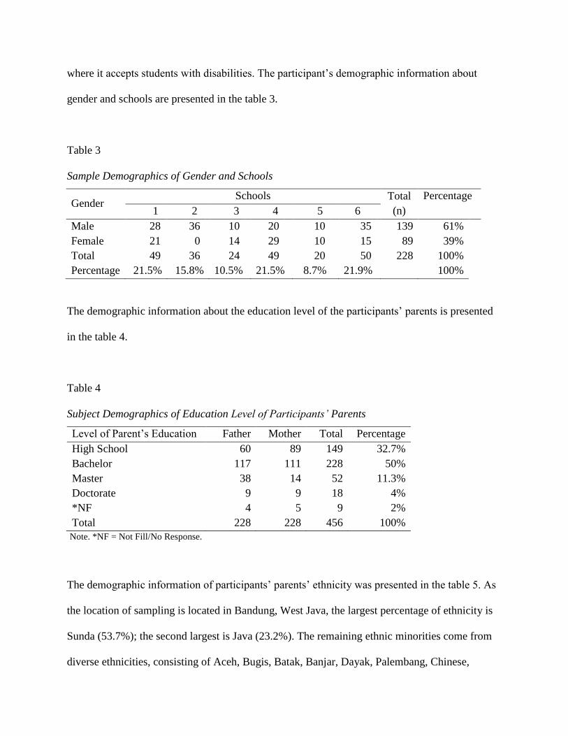
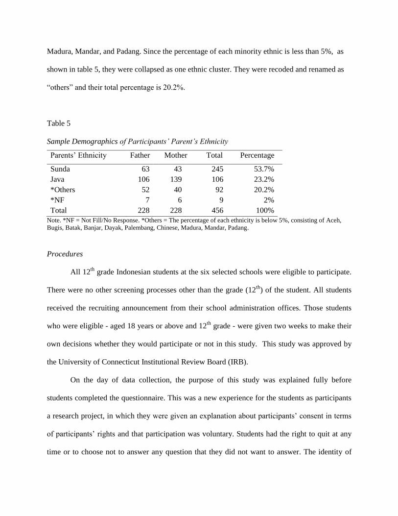


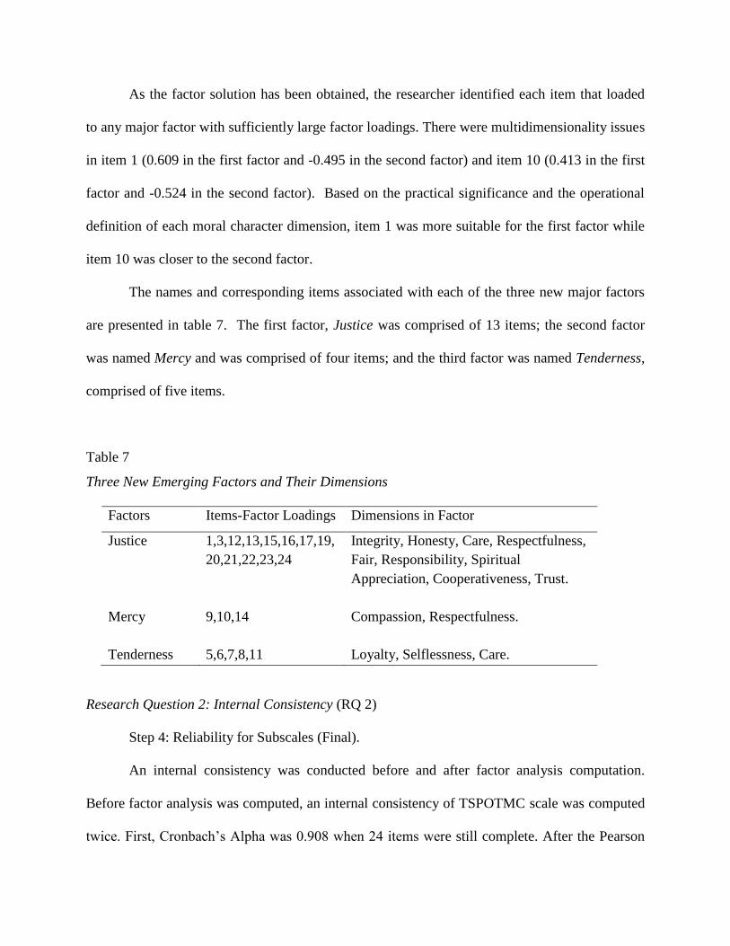


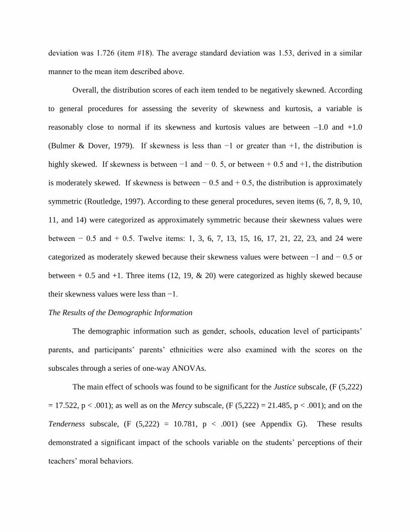


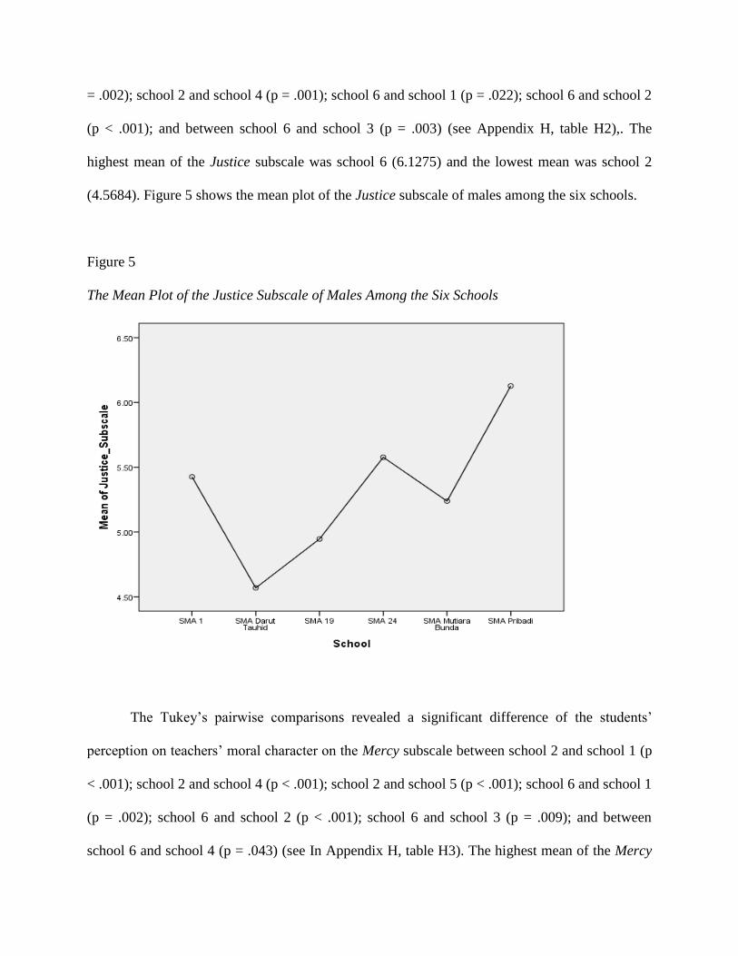
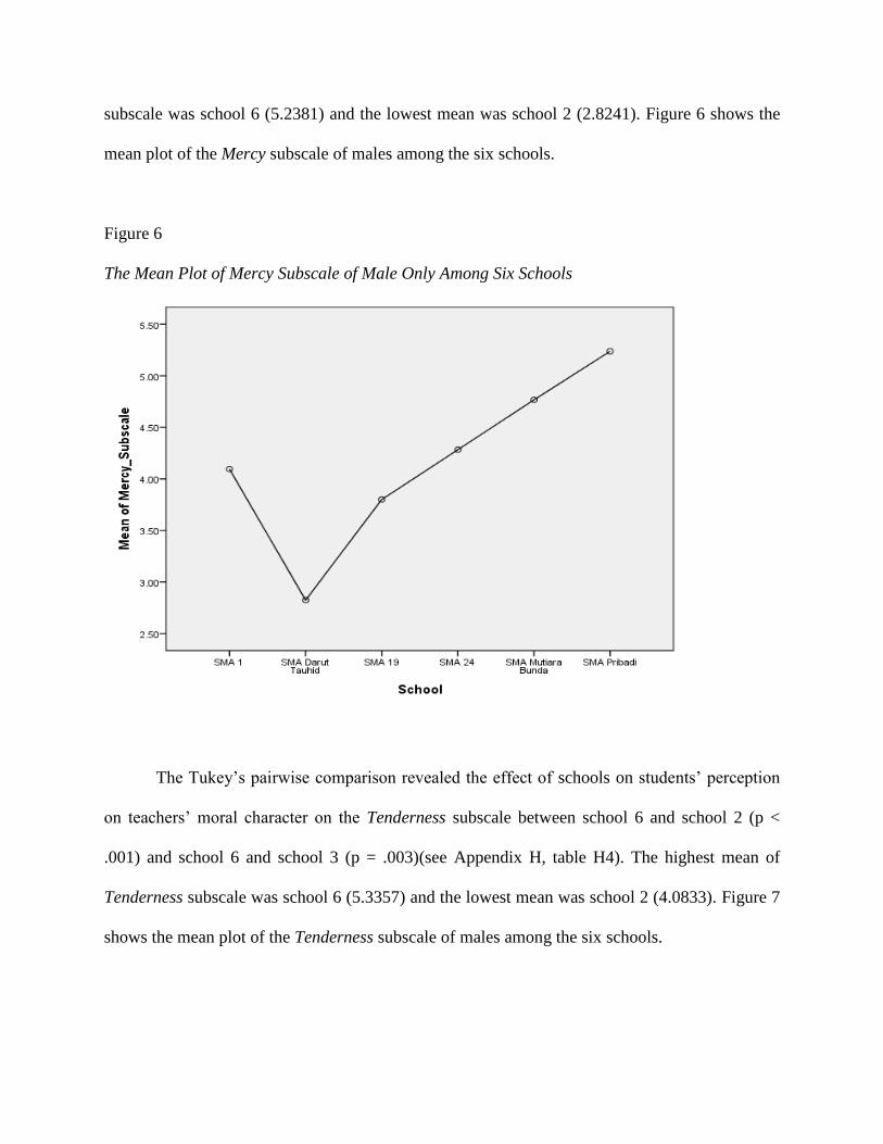


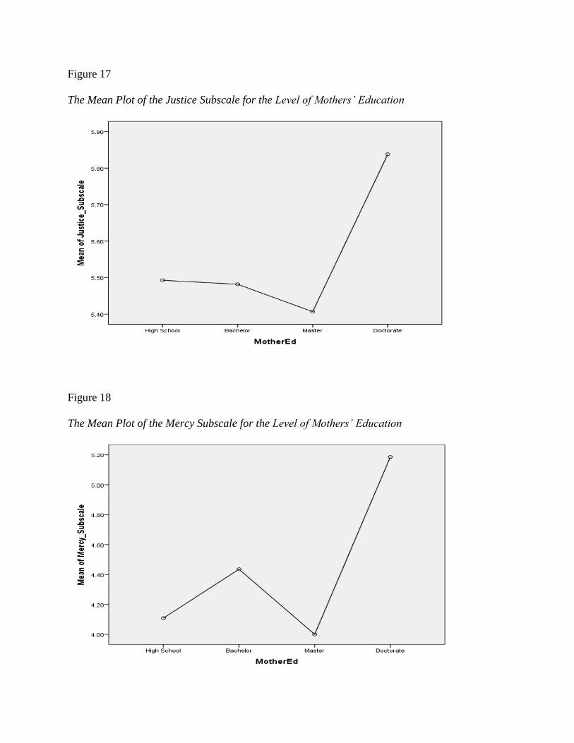

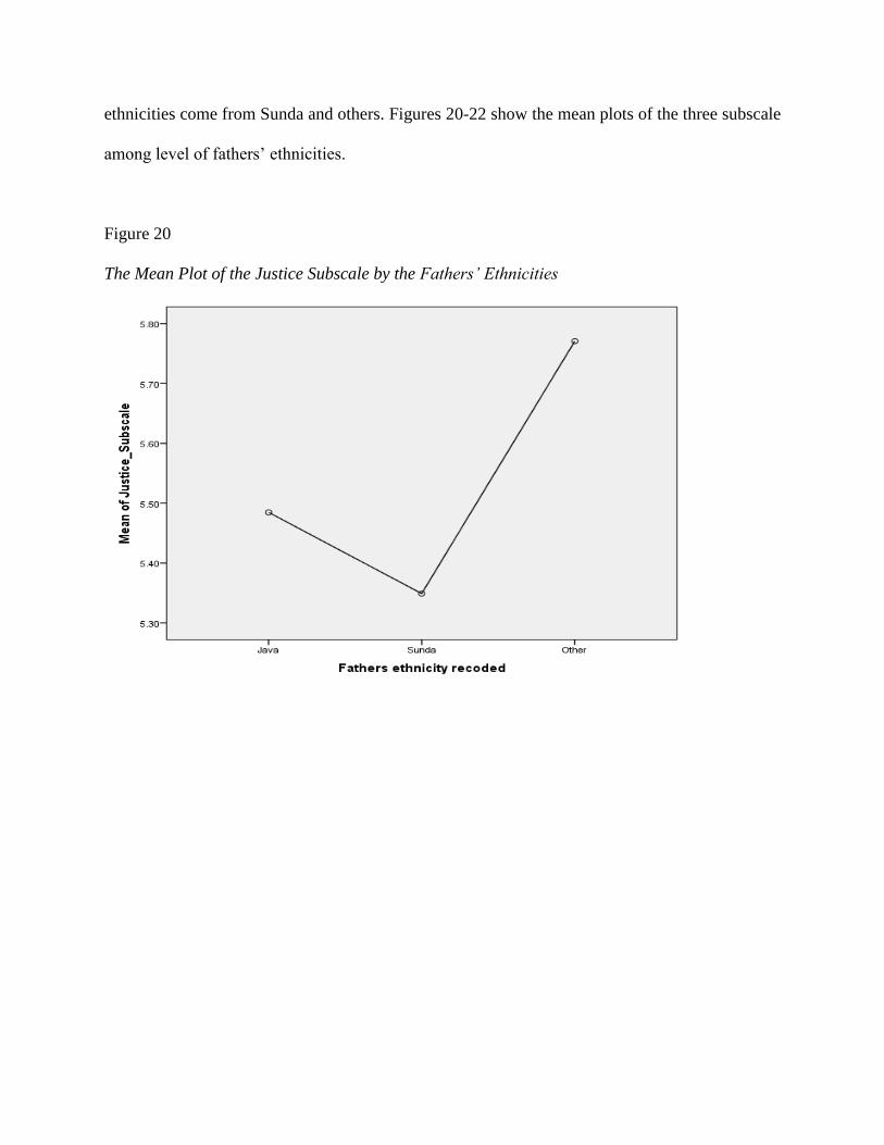


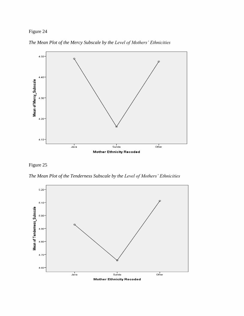


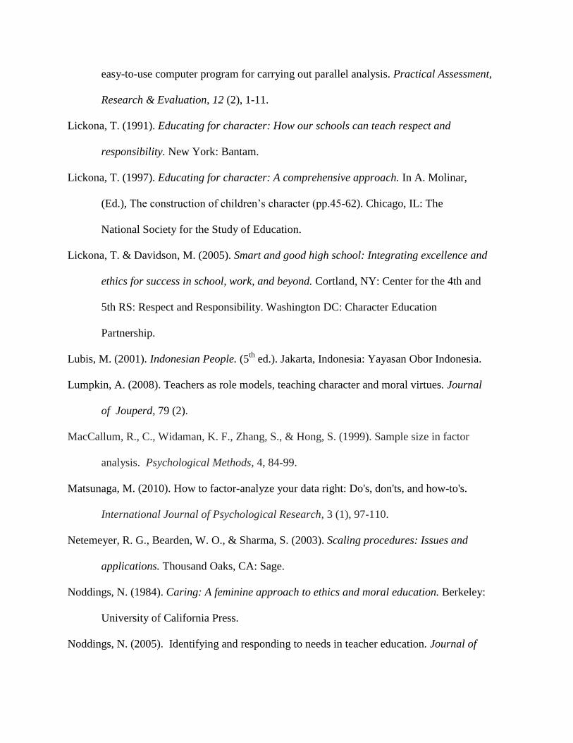
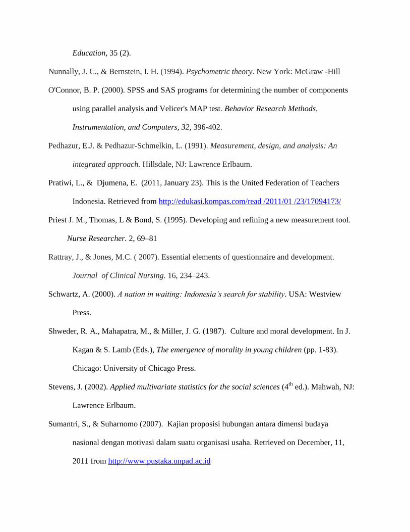


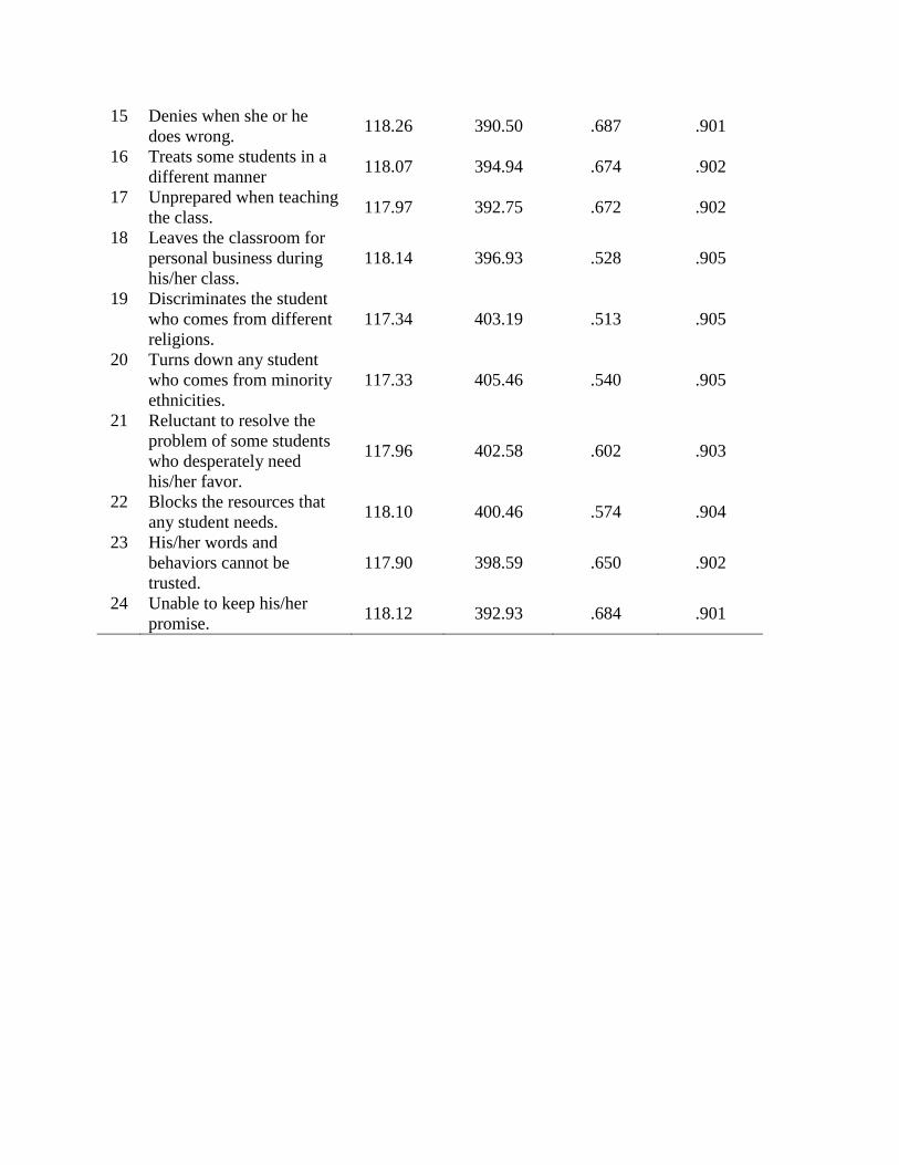


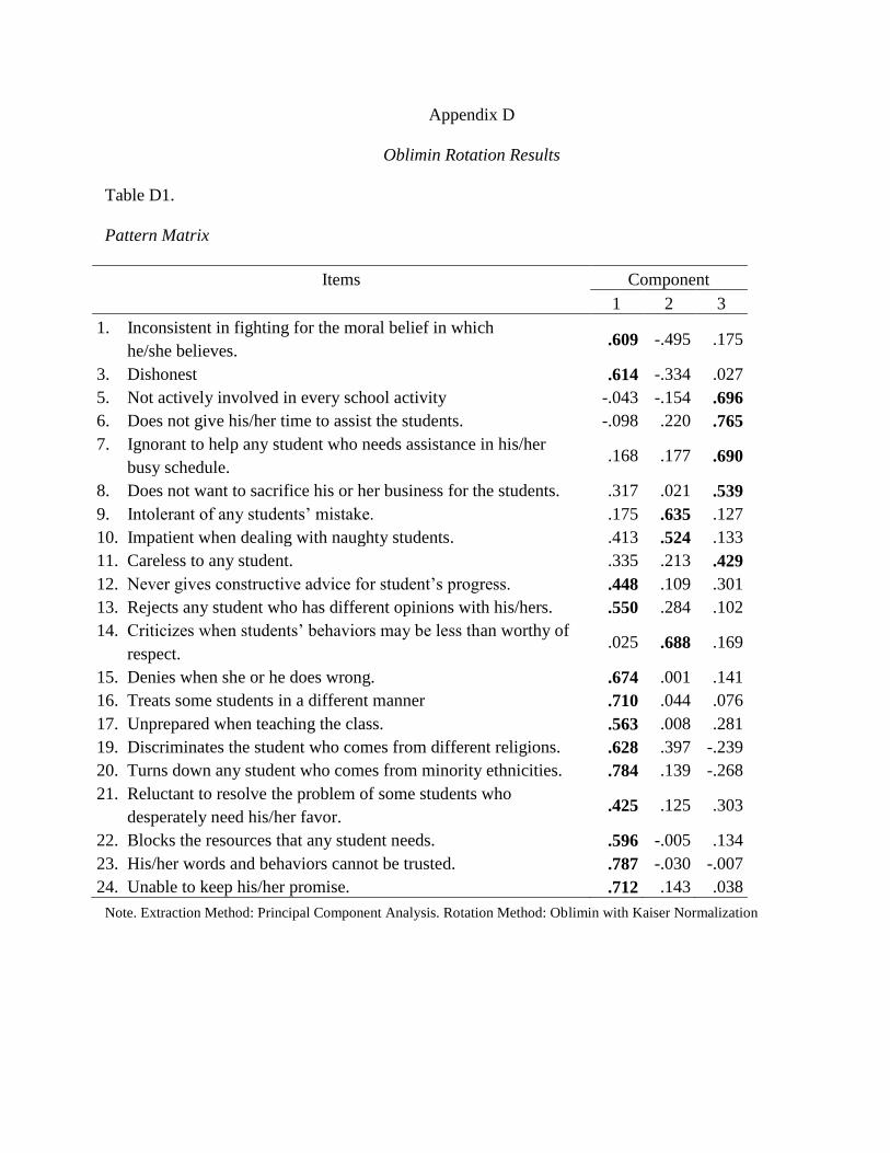

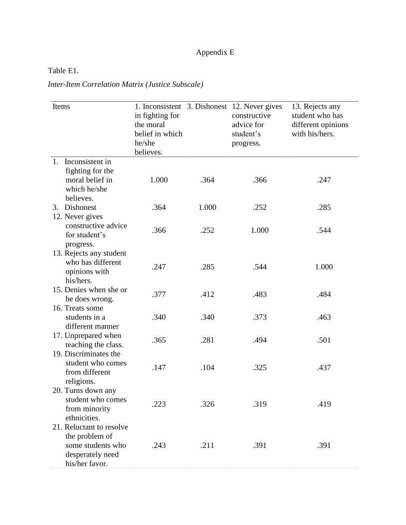


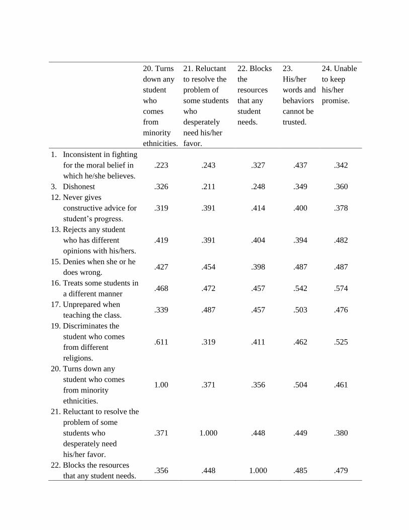
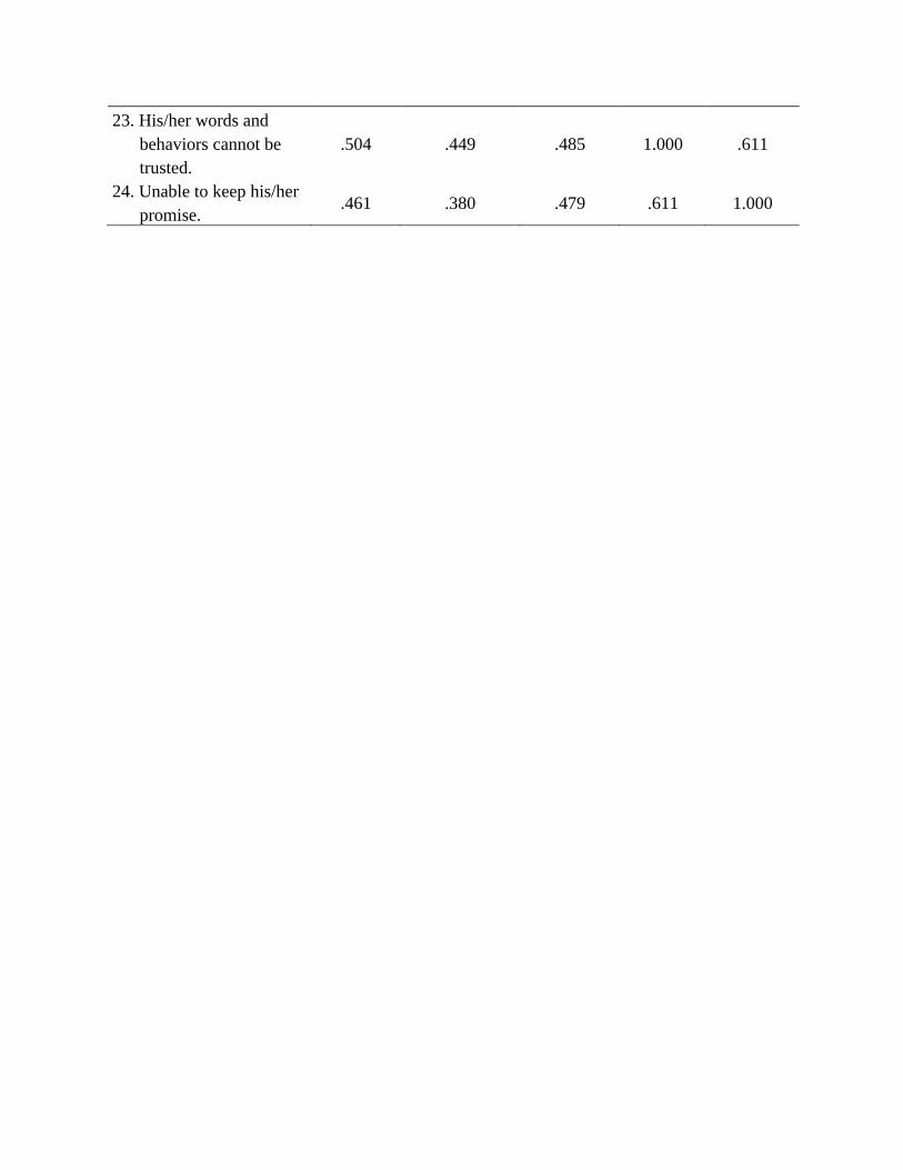


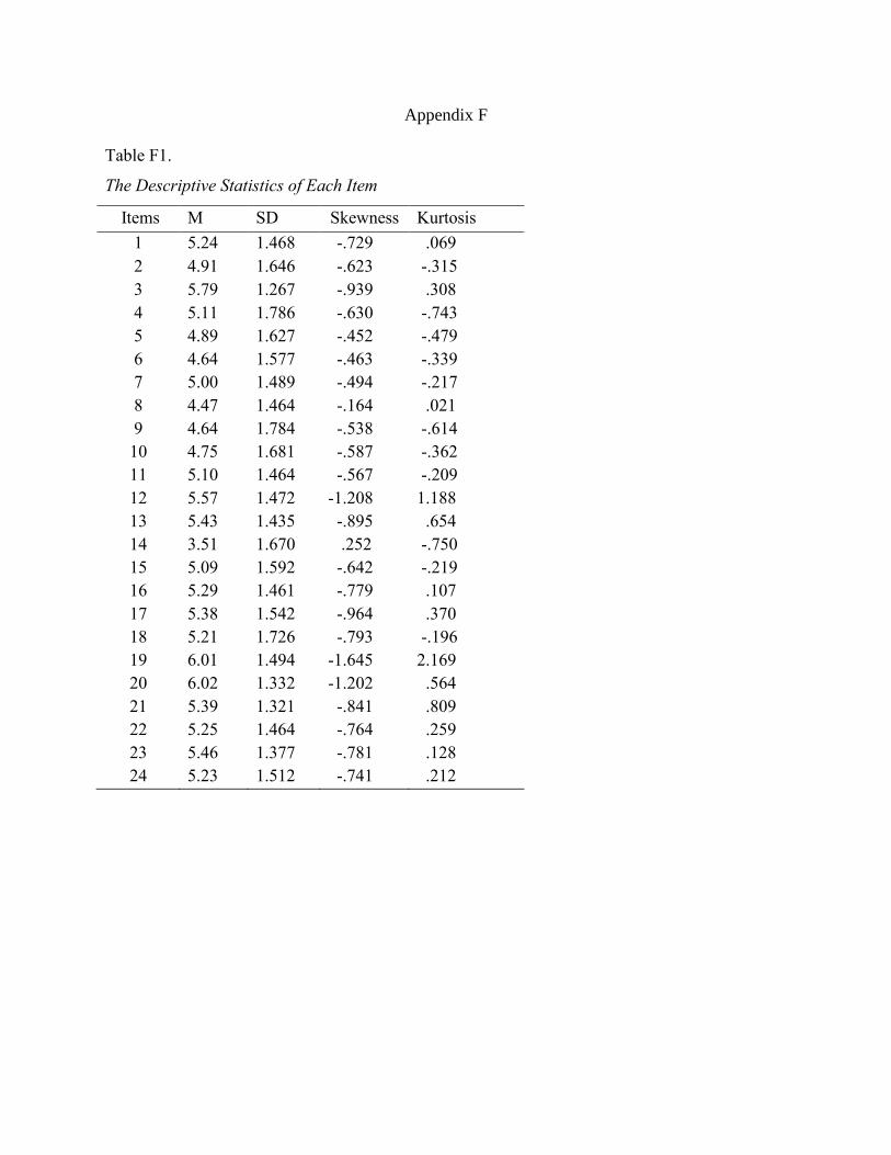


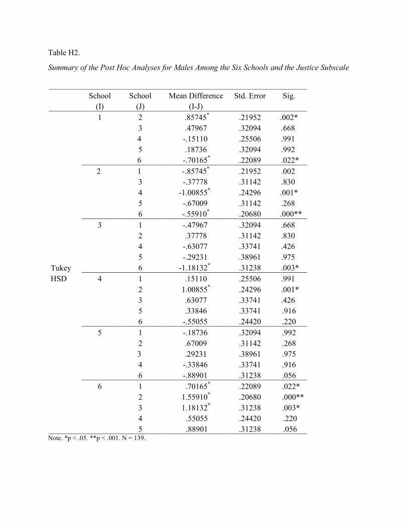
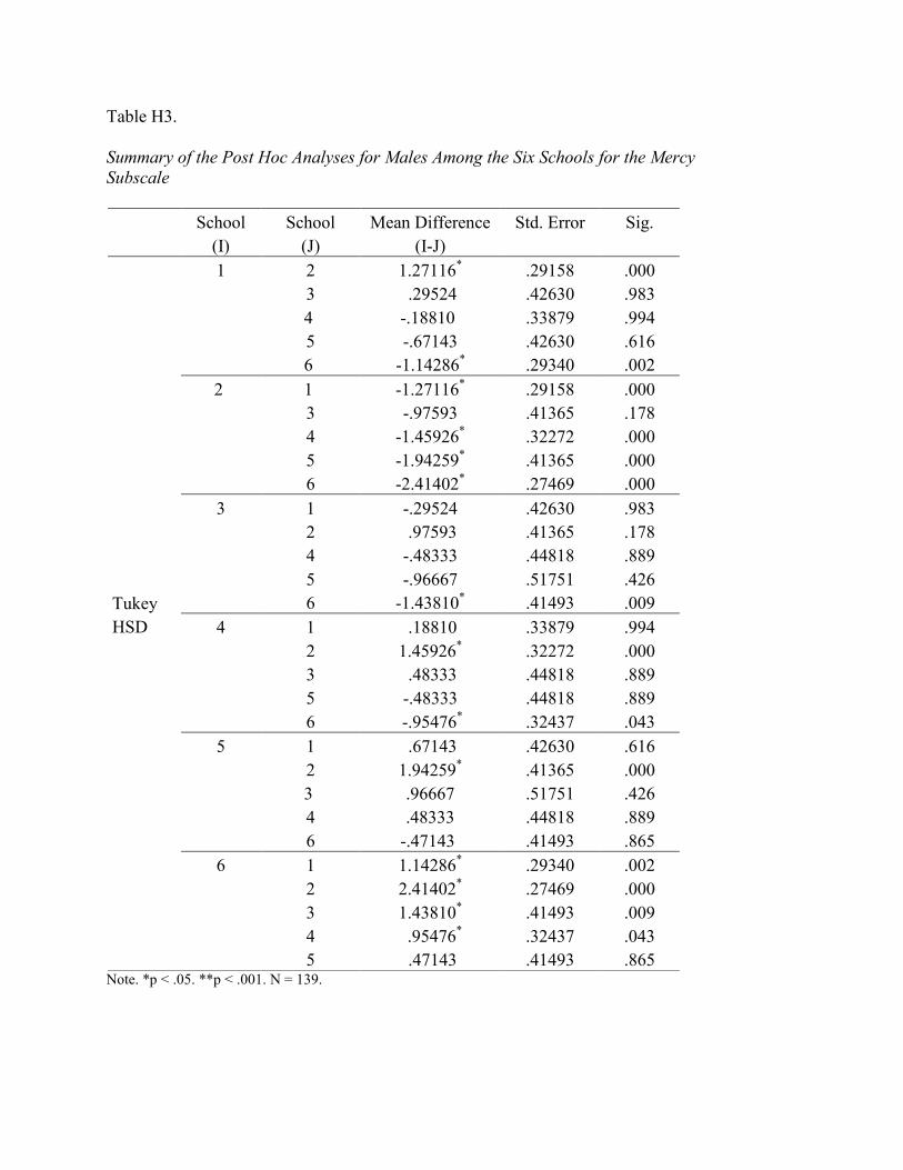

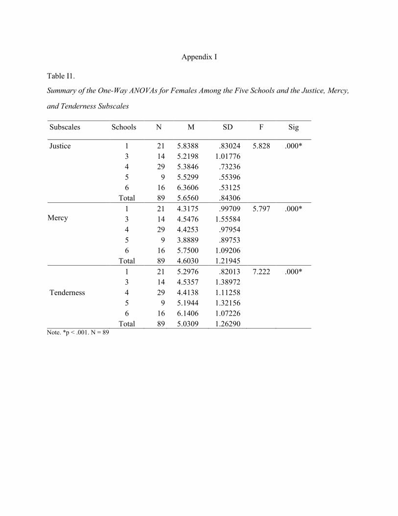


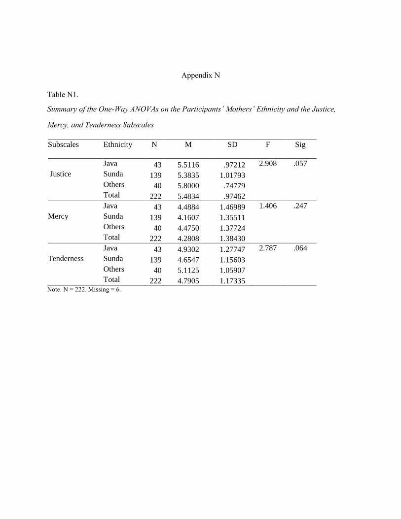


![Moral Realism, Moral Relativism, Moral Rules [Oddie]](https://static.documents.pub/doc/80x56/577cd1091a28ab9e78937559/moral-realism-moral-relativism-moral-rules-oddie.jpg)


